Limit setting and statisticsJory Sonneveld

1jory.sonneveld@cern.ch

An example of a “limit”in high energy physics

From CMS-SUS-16-033

“Limit” on gluino+LSP mass

2

Another example of a “limit” in HEPLimit on the Higgs cross section in terms of the Standard Model expectation

CL?

→ confidence level

3https://www-cdf.fnal.gov/physics/new/hdg/Plain_English_files/higgs-limits-march2009.gif

Where does this ‘‘limit’’ come from?A contour line:

A theory prediction:

An upper limit: 4

https://twiki.cern.ch/twiki/bin/view/LHCPhysics/SUSYCrossSections13TeVgluglu

See T. Junk http://arxiv.org/abs/hep-ex/9902006

The contour lineFor each mass point:

● An upper limit from CMS● An upper limit from

MadAnalysis ( → color)● A theory prediction for a cross

section a KK gluon mass of twice the KK quark mass

● A theory prediction for a cross section for a KK gluon mass of four times the KK quark mass

● The bin for which the upper limit was computed

5from here

The theory prediction

Depends on:

● Model● PDFs● Tool (Pythia, NLLFast)● Masses of other particles● ... 6

https://twiki.cern.ch/twiki/bin/view/LHCPhysics/SUSYCrossSections#SUSY_Cross_Sections_using_13_14

The upper limit

CL: confidence level

X: a test statistic or discriminant

b: number of expected background events (estimated)

nobs: number of observed events in data (counted)

s: varied until a certain confidence level, e.g. 95%, is reached →

The cross section is related to the number of events: , or xsec * efficiency * luminosity 7

See T. Junk http://arxiv.org/abs/hep-ex/9902006

(s=0)

s: varied until a certain confidence level, e.g. 95%, is reached →

So set for example CL := 0.95 → compute upper limit by solving for s

Confidence level and upper limit

8

A p-valueProbability that (in this case) background gives at least 8 observed events if background is correct, or an overfluctuation would give >= 8 events:

Not the probability that the background is true! 9

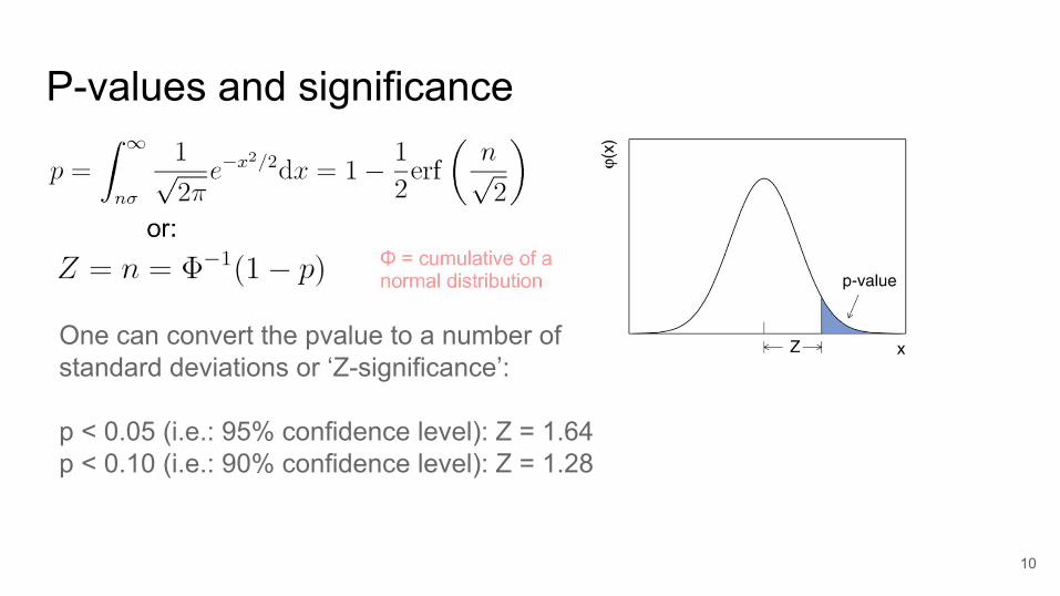
P-values and significance

10

One can convert the pvalue to a number of standard deviations or ‘Z-significance’:

p < 0.05 (i.e.: 95% confidence level): Z = 1.64p < 0.10 (i.e.: 90% confidence level): Z = 1.28

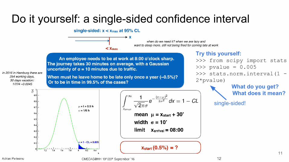
Do it yourself: a single-sided confidence interval

11

Try this yourself:>>> from scipy import stats>>> pvalue = 0.005>>> stats.norm.interval(1 - 2*pvalue) What do you get?

What does it mean?

single-sided!

A confidence interval

12

http://www.sjsu.edu/faculty/gerstman/StatPrimer/t-table.pdf

>>> number_of_sigma = stats.norm.interval(1 - 2*tail)[1]>>> number_of_sigma2.5758293035489004>>> minutes = number_of_sigma*10>>> total = minutes + 30>>> total55.758293035489004

Testing hypotheses and discrimination

13

Accept null hypothesis H0

Reject null hypothesis

What can go wrong here?

See also the book: Statistical Data Analysis by Glenn Cowan

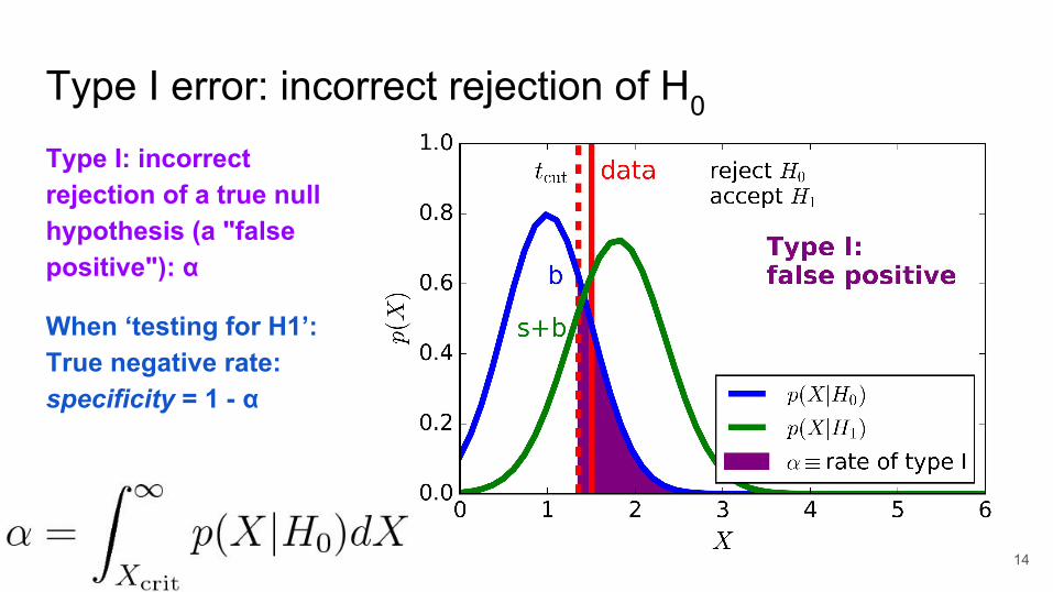
Type I error: incorrect rejection of H0

Type I: incorrect rejection of a true null hypothesis (a "false positive"): α

When ‘testing for H1’:True negative rate: specificity = 1 - α

14

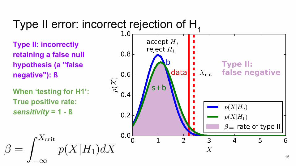
Type II error: incorrect rejection of H1

Type II: incorrectly retaining a false null hypothesis (a "false negative"): ß

When ‘testing for H1’:True positive rate: sensitivity = 1 - ß

15

Type I and Type II errorsTesting a hypothesis:

H0 null hypothesis: user is logging in

H1 alternative hypothesis: imposter is logging in

I. classify authorized users as impostersincorrect rejection of a true null hypothesis (a "false positive"): α

II. classify imposters as authorized usersincorrectly retaining a false null hypothesis (a "false negative"): ß

True positive rate: sensitivity = 1 - ßTrue negative rate: specificity = 1 - α

16

srcImposter

m(Higgs) = 220 GeV?

17https://profmattstrassler.files.wordpress.com/2011/12/hcp_h2zz1.pnghttps://profmattstrassler.com/articles-and-posts/the-higgs-particle/the-standard-model-higgs/seeking-and-studying-the-standard-model-higgs-particle/

How can we easily recognize a ‘fake’ signal? And why?

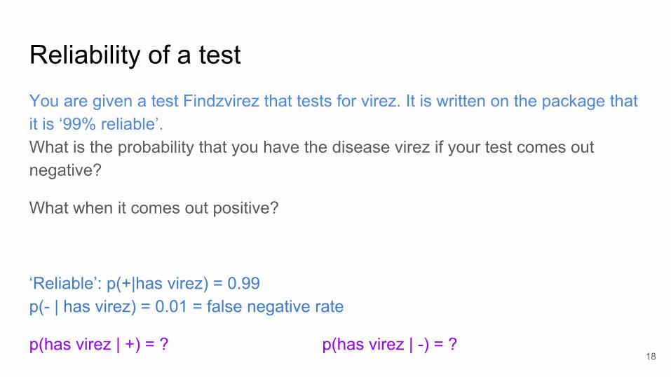
Reliability of a testYou are given a test Findzvirez that tests for virez. It is written on the package that it is ‘99% reliable’.What is the probability that you have the disease virez if your test comes out negative?

What when it comes out positive?

‘Reliable’: p(+|has virez) = 0.99p(- | has virez) = 0.01 = false negative rate

p(has virez | +) = ? p(has virez | -) = ?18

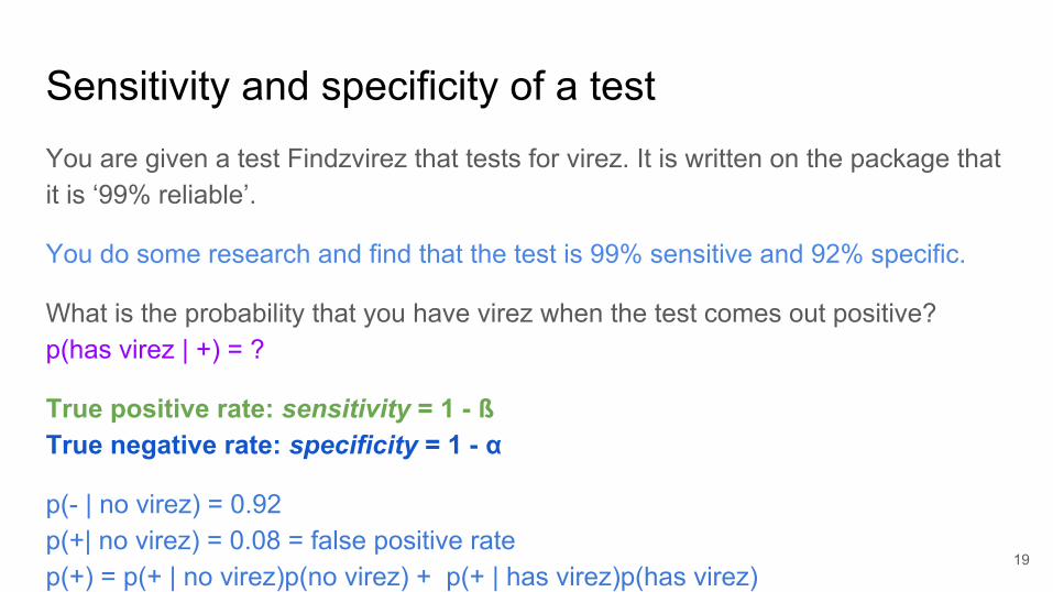
Sensitivity and specificity of a testYou are given a test Findzvirez that tests for virez. It is written on the package that it is ‘99% reliable’.

You do some research and find that the test is 99% sensitive and 92% specific.

What is the probability that you have virez when the test comes out positive?p(has virez | +) = ?

True positive rate: sensitivity = 1 - ßTrue negative rate: specificity = 1 - α

p(- | no virez) = 0.92p(+| no virez) = 0.08 = false positive ratep(+) = p(+ | no virez)p(no virez) + p(+ | has virez)p(has virez)

19

Probabilities and Bayes’ theoremSolve this using Bayes’ theorem: the probability of an event based on prior knowledge of conditions that may be related to the event

Many false positives: airport security screening

US breast cancer mammography: false positive rate 15%→ After 10 years of screening, half of the American population has one false positive

20

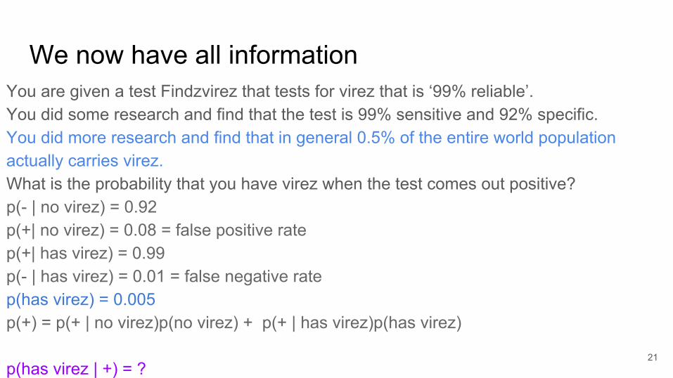
We now have all informationYou are given a test Findzvirez that tests for virez that is ‘99% reliable’. You did some research and find that the test is 99% sensitive and 92% specific.You did more research and find that in general 0.5% of the entire world population actually carries virez.What is the probability that you have virez when the test comes out positive?p(- | no virez) = 0.92p(+| no virez) = 0.08 = false positive ratep(+| has virez) = 0.99p(- | has virez) = 0.01 = false negative ratep(has virez) = 0.005p(+) = p(+ | no virez)p(no virez) + p(+ | has virez)p(has virez)

p(has virez | +) = ?21

No need to worry on testing positive What is the probability that you have virez when the test comes out positive?p(+| no virez) = 0.08 = false positive ratep(+| has virez) = 0.99p(has virez) = 0.005p(+) = p(+ | no virez)p(no virez) + p(+ | has virez)p(has virez)

p(has virez | +) = p(+ | has virez)p(has virez) / p(+)

= 0.99*0.005 / (0.08*0.995 + 0.99*0.005) = 0.0585452395

22Don’t worry, but do go for your next (much better) test =)

The upper limit

CL: confidence level

X: a test statistic or discriminant

b: number of expected background events (estimated)

nobs: number of observed events in data (counted)

s: varied until a certain confidence level, e.g. 95%, is reached →

The cross section is related to the number of events: , or xsec * efficiency * luminosity 23

See T. Junk http://arxiv.org/abs/hep-ex/9902006

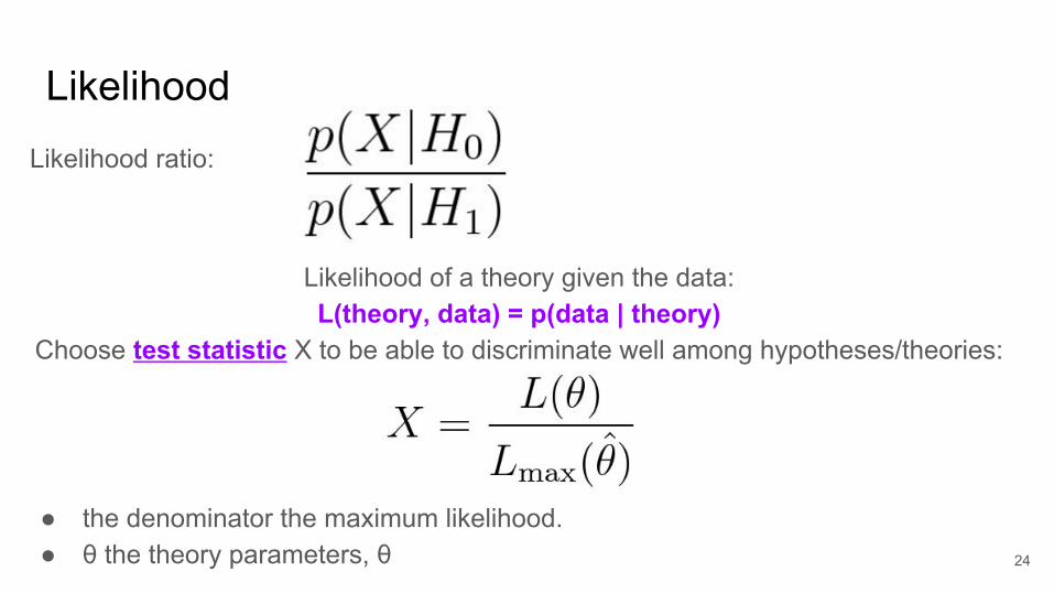
LikelihoodLikelihood ratio:

Likelihood of a theory given the data: L(theory, data) = p(data | theory)

Choose test statistic X to be able to discriminate well among hypotheses/theories:

● the denominator the maximum likelihood.● θ the theory parameters, θ 24

Example of a test statistic: likelihood ratio

General likelihood:

L(data | θ ) = Poisson(data | s(θ) + b(θ) ) ・ p( θ | θ )

Poisson distribution (counting experiment)Can be used to generate pseudodata 25

Likelihood~χ2

~

Smearing from nuisance parameters:Gaussian, lognormal pdf

Likelihood methods

nuisance parameters: unknown parameters not interesting for the measurement, like detector resolution, uncertainty in backgrounds, background shape modeling, other systematic uncertainties

Frequentist: constrain likelihood nuisance parameters with e.g. control sample:

L(data, control sample | θ) = L( data | θ, s, b) L(control sample | θ)

Bayesian: integrate analytically, numerically, with Markov Chain Monte Carlo

Hybrid: integrate or marginalize the likelihood function over the nuisance parameters, then frequentist method

26

Frequentist method: toy experimentsExample: Fittino toy ‘fits’ to obtain χ2 distribution

27https://arxiv.org/abs/1508.05951Eur.Phys.J. C76 (2016) no.2, 96

H0 background hypothesis

Signal +background hypothesis

H1 signal hypothesis

P-value: fraction of toys > tobs

p = 374/105 = 3.7±0.2%

Z = 2.7

Bayesian limits

28

Systematic uncertainties

Prior: usually flat, 0 for s <= 0

Nuisance parameters x

Normalization constant

95% CL upper limit on amount of signal events

Data or pseudodata

Signal s(θ, x) and background b(x)

Posterior density

Sometimes:μs with signal strength modifier μ

Bayesian priors in particle physicsTheory: Allzymmetric(a, other parameters).

Experiment: observable A can only take the values 0 <= A <= 20.You compute that for Allzymmetric:

0 <= A <= 20 would imply 0 <= a <= 2000.

You choose a prior π(θ) with θ your Allzymmetric theory parameters such that

π(θ) = 1, 0 <= a <= 2000;π(θ) = 0 otherwise.

For example, you do not look at any SUSY parameters that predict ΩDM > 0.12 (see Table 3 of https://arxiv.org/pdf/1502.01589v3.pdf from the Planck results)

29

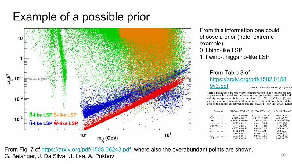
Example of a possible prior

30From Fig. 7 of https://arxiv.org/pdf/1505.06243.pdf where also the overabundant points are shown.G. Belanger, J. Da Silva, U. Laa, A. Pukhov

From Table 3 of https://arxiv.org/pdf/1502.01589v3.pdf

From this information one could choose a prior (note: extreme example):0 if bino-like LSP1 if wino-, higgsino-like LSP

Bayesian posterior density: a pMSSM example

31

See also JHEP 10 (2016) 129arXiv:1606.03577http://cms-results.web.cern.ch/cms-results/public-results/publications/SUS-15-010/index.html

Note: NO dark matter constraints in here!

p(θ|d) ∝ L(d CMS−SUSY |θ)L(d pre−CMS−SUSY |θ)p(θ)

Aside: these densities/probabilities went down

32

Prior used in CMS pMSSM interpretation

33

The upper limit

CL: confidence level

X: a test statistic or discriminant

b: number of expected background events (estimated)

nobs: number of observed events in data (counted)

s: varied until a certain confidence level, e.g. 95%, is reached →

The cross section is related to the number of events: , or xsec * efficiency * luminosity 34

See T. Junk http://arxiv.org/abs/hep-ex/9902006

What is CLs?Why not CLs+b?

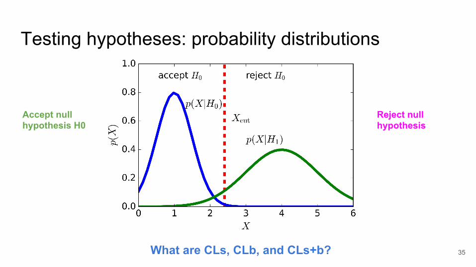
Testing hypotheses: probability distributions

35

Accept null hypothesis H0

Reject null hypothesis

What are CLs, CLb, and CLs+b?

Confidence level: CLs, CLb, and CLs+b

CLs = CLs+b/CLb36

Another example of a “limit”Limit on the Higgs cross section in terms of the Standard Model expectation

● Dashed line: expected limit● Solid line: observed limit

37https://www-cdf.fnal.gov/physics/new/hdg/Plain_English_files/higgs-limits-march2009.gif

Many results combined

We (outside the experiment) usually are not able to combine results without knowing all correlations

38

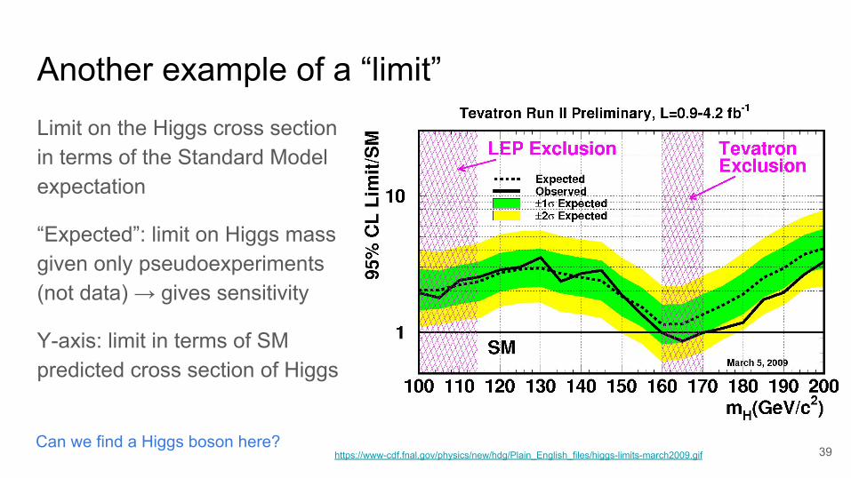
Another example of a “limit”Limit on the Higgs cross section in terms of the Standard Model expectation

“Expected”: limit on Higgs mass given only pseudoexperiments (not data) → gives sensitivity

Y-axis: limit in terms of SM predicted cross section of Higgs

39https://www-cdf.fnal.gov/physics/new/hdg/Plain_English_files/higgs-limits-march2009.gifCan we find a Higgs boson here?

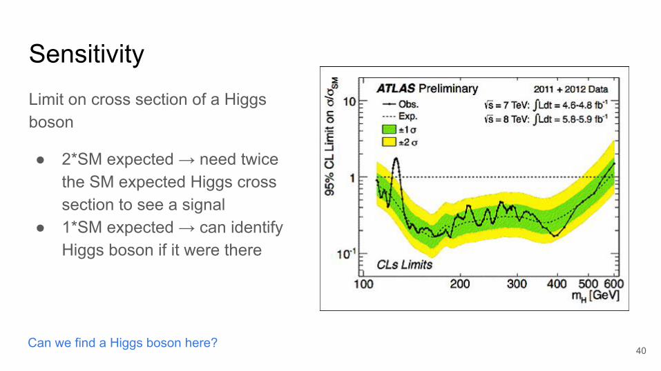
SensitivityLimit on cross section of a Higgs boson

● 2*SM expected → need twice the SM expected Higgs cross section to see a signal

● 1*SM expected → can identify Higgs boson if it were there

40Can we find a Higgs boson here?

A signal● Observed > expected:

upward fluctuation, signal

● Observed < expected: downward fluctuation, exclusion

One expects ⅔ of observed limit to fall within bands of pseudoexperiments.

What do we see here? 41Did we exclude? Discover?

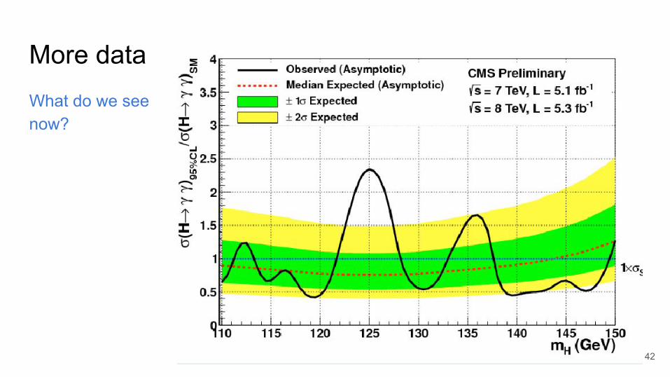
More dataWhat do we seenow?

42

Methods at LEP, Tevatron, LHC

43https://cdsweb.cern.ch/record/1375842/files/ATL-PHYS-PUB-2011-011.pdf

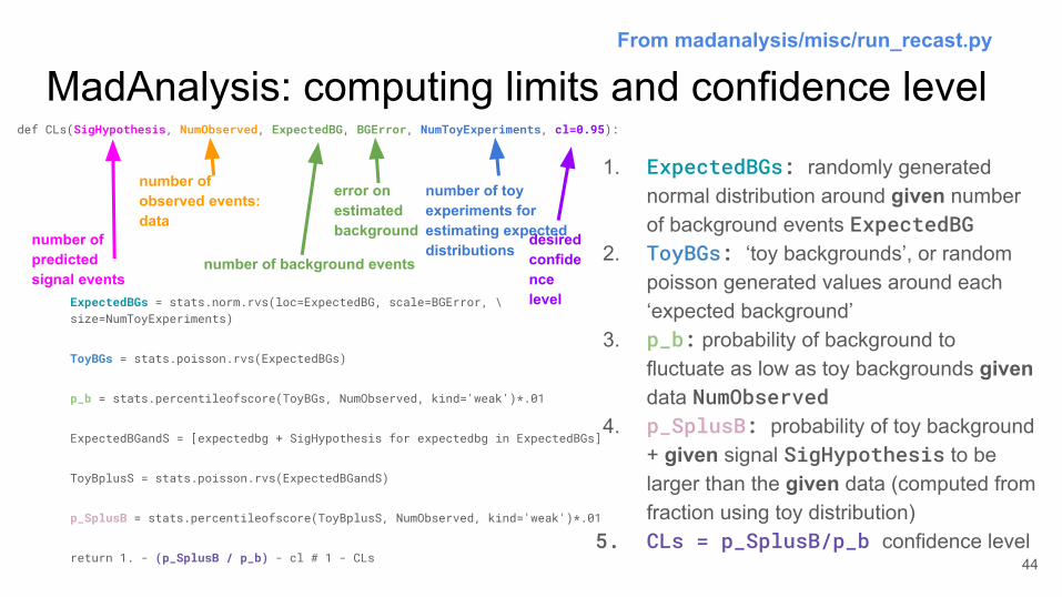
def CLs(SigHypothesis, NumObserved, ExpectedBG, BGError, NumToyExperiments, cl=0.95):

ExpectedBGs = stats.norm.rvs(loc=ExpectedBG, scale=BGError, \size=NumToyExperiments)

ToyBGs = stats.poisson.rvs(ExpectedBGs)

p_b = stats.percentileofscore(ToyBGs, NumObserved, kind='weak')*.01

ExpectedBGandS = [expectedbg + SigHypothesis for expectedbg in ExpectedBGs]

ToyBplusS = stats.poisson.rvs(ExpectedBGandS)

p_SplusB = stats.percentileofscore(ToyBplusS, NumObserved, kind='weak')*.01

return 1. - (p_SplusB / p_b) - cl # 1 - CLs

1. ExpectedBGs: randomly generated normal distribution around given number of background events ExpectedBG

2. ToyBGs: ‘toy backgrounds’, or random poisson generated values around each ‘expected background’

3. p_b: probability of background to fluctuate as low as toy backgrounds given data NumObserved

4. p_SplusB: probability of toy background + given signal SigHypothesis to be larger than the given data (computed from fraction using toy distribution)

5. CLs = p_SplusB/p_b confidence level

MadAnalysis: computing limits and confidence level

44

number of background events

number of observed events: data

number of predicted signal events

error on estimated background

number of toy experiments for estimating expected distributions

desired confidence level

From madanalysis/misc/run_recast.py

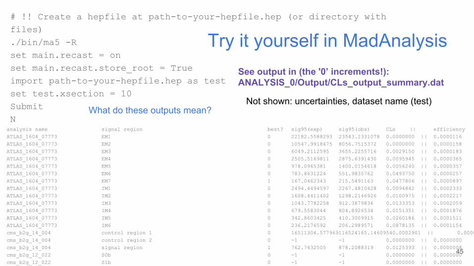
Try it yourself in MadAnalysis# !! Create a hepfile at path-to-your-hepfile.hep (or directory with files)./bin/ma5 -Rset main.recast = onset main.recast.store_root = Trueimport path-to-your-hepfile.hep as testset test.xsection = 10SubmitN

# dataset name analysis name signal region best? sig95(exp) sig95(obs) CLs || efficiency stat. unc. syst. unc. tot. unc. test ATLAS_1604_07773 EM1 0 22182.5588293 23543.2331078 0.0000000 || 0.0000116 0.0017029 0.0000000 0.0017029 test ATLAS_1604_07773 EM2 0 10547.9918475 8056.7515372 0.0000000 || 0.0000158 0.0019838 0.0000000 0.0019838 test ATLAS_1604_07773 EM3 0 6049.2112595 3655.2255716 0.0029150 || 0.0000183 0.0021346 0.0000000 0.0021346 test ATLAS_1604_07773 EM4 0 2505.5169811 2875.6391430 0.0095945 || 0.0000365 0.0030188 0.0000000 0.0030188 test ATLAS_1604_07773 EM5 0 978.0965381 1400.0154618 0.0056240 || 0.0000357 0.0029843 0.0000000 0.0029843 test ATLAS_1604_07773 EM6 0 783.8631224 551.9835762 0.0493750 || 0.0000257 0.0025339 0.0000000 0.0025339 test ATLAS_1604_07773 EM7 1 167.0462343 215.5491163 0.0477806 || 0.0000897 0.0047294 0.0000000 0.0047294 test ATLAS_1604_07773 IM1 0 2494.4494597 2267.4810428 0.0094842 || 0.0002333 0.0076281 0.0000000 0.0076281 test ATLAS_1604_07773 IM2 0 1608.4411402 1298.2146926 0.0100975 || 0.0002217 0.0074357 0.0000000 0.0074357 test ATLAS_1604_07773 IM3 0 1043.7782258 912.3879836 0.0133353 || 0.0002059 0.0071663 0.0000000 0.0071663 test ATLAS_1604_07773 IM4 0 679.5583044 804.8926534 0.0151351 || 0.0001876 0.0068411 0.0000000 0.0068411 test ATLAS_1604_07773 IM5 0 342.8603425 410.3009915 0.0260186 || 0.0001511 0.0061393 0.0000000 0.0061393 test ATLAS_1604_07773 IM6 0 236.2176592 206.2989571 0.0878135 || 0.0001154 0.0053653 0.0000000 0.0053653 test cms_b2g_14_004 control region 1 0 16511304.577969116524165.14609540.0002901 || 0.0000029 0.0008454 0.0000000 0.0008454 test cms_b2g_14_004 control region 2 0 -1 -1 0.0000000 || 0.0000000 0.0000000 0.0000000 0.0000000 test cms_b2g_14_004 signal region 1 762.7432505 878.2088319 0.0125393 || 0.0000008 0.0004411 0.0000000 0.0004411 test cms_b2g_12_022 S0b 0 -1 -1 0.0000000 || 0.0000000 0.0000000 0.0000000 0.0000000 test cms_b2g_12_022 S1b 0 -1 -1 0.0000000 || 0.0000000 0.0000000 0.0000000

45

Not shown: uncertainties, dataset name (test)What do these outputs mean?

See output in (the '0’ increments!): ANALYSIS_0/Output/CLs_output_summary.dat

Backup

46

References and links

47

● T. Junk http://arxiv.org/abs/hep-ex/9902006● A.L Read on CLs Journal of Physics G: Nuclear and Particle Physics 28 no. 10, (2002) 2693● Statistical Data Analysis by Glenn Cowan● Likelihoods https://cdsweb.cern.ch/record/1375842/files/ATL-PHYS-PUB-2011-011.pdf● Simplified likelihoods in CMS https://cds.cern.ch/record/2242860/ ● Data Analysis, a Baysian Tutorial by Sivia and Skilling● Slides by Luca Lista● Azatov, Contino, Galloway https://arxiv.org/pdf/1202.3415v3.pdf● Wikipedia on sensitivity, specificity, Bayes' theorem, type I and II errors, …● Ipython notebook examples: https://github.com/jupyter/jupyter/wiki/A-gallery-of-interesting-Jupyter-Notebooks#machine-learning-statistics-and-probability

And also:● How Randomness Rules Our Lives by Leonard Mlodinow● Critical Mass by Philip Ball● Thinking, Fast and Slow by Daniel Kahneman

Try it yourself: three doors problemOne student plays the contestant, and another, the host. Label three paper cups #1, #2, and #3. While the contestant looks away, the host randomly hides a penny under a cup by throwing a die until a 1, 2, or 3 comes up. Next, the contestant randomly points to a cup by throwing a die the same way. Then the host purposely lifts up a losing cup from the two unchosen. Lastly, the contestant "stays" and lifts up his original cup to see if it covers the penny. Play "not switching" two hundred times and keep track of how often the contestant wins.

Then test the other strategy. Play the game the same way until the last instruction, at which point the contestant instead "switches" and lifts up the cup not chosen by anyone to see if it covers the penny. Play "switching" two hundred times, also.

48https://en.wikipedia.org/wiki/Monty_Hall_problemhttp://marilynvossavant.com/game-show-problem/

Note: I would simulate this =)

Change door! DOOR 1 DOOR 2 DOOR 3 RESULT

GAME 1 AUTO GOAT GOAT Switch and you lose.

GAME 2 GOAT AUTO GOAT Switch and you win.

GAME 3 GOAT GOAT AUTO Switch and you win.

GAME 4 AUTO GOAT GOAT Stay and you win.

GAME 5 GOAT AUTO GOAT Stay and you lose.

GAME 6 GOAT GOAT AUTO Stay and you lose.49

Confidence level: confidence intervalsWant to measure an unknown parameter θ:

We do not know we know θ, but if we know the pdf g for an estimator for a given value of θ, we can define:

● The probability to find θ in an interval higher than a lower value α:

● The probability to find θ in an interval lower than a higher value β:

● From this we find the probability to have a true value θ in the interval [a,b] → 50

See also the book: Statistical Data Analysis by Glenn Cowan

Confidence interval: single-sided

A one-sided confidence interval or limit is the lower limit a on θ so that

a < θ

with the probability 1 - α

or the upper limit b on θ so that

θ < b

with the probability 1 - β.

A central interval can be defined with probability 1 - α - β51

False positive rate

False negative rate

Nuisance parametersnuisance parameters: unknown parameters not interesting for the measurement:

● detector resolution● uncertainty in backgrounds● background shape modeling● other systematic uncertainties● ...

Then one can:

● Add the nuisance parameters to your likelihood model (easier to incorporate in a fit than in upper limits)

● “Integrate it away” (Bayesian way) 52

Likelihood methodsFrequentist: constrain likelihood nuisance parameters with e.g. control sample:

L(data, control sample | θ) = L( data | θ, s, b) L(control sample | θ)

a large fraction (68% or 95%, usually) of the experiments contain the fixed but unknown true value within the confidence interval [θest - δ1 , θ

est + δ2 ]

Bayesian: integrate analytically, numerically, with Markov Chain Monte Carlo

The posterior PDF for θ is maximum at θ est and its integral is 68% within the range [θest - δ1 , θ

est + δ2 ]

Hybrid: integrate or marginalize the likelihood function over the nuisance parameters 53