lifting and wavelets: a factorization method
TRANSCRIPT

University of Texas at El PasoDigitalCommons@UTEP
Open Access Theses & Dissertations
2012-01-01
Lifting and Wavelets: A Factorization MethodAdrian DelgadoUniversity of Texas at El Paso, [email protected]
Follow this and additional works at: https://digitalcommons.utep.edu/open_etdPart of the Mathematics Commons
This is brought to you for free and open access by DigitalCommons@UTEP. It has been accepted for inclusion in Open Access Theses & Dissertationsby an authorized administrator of DigitalCommons@UTEP. For more information, please contact [email protected].
Recommended CitationDelgado, Adrian, "Lifting and Wavelets: A Factorization Method" (2012). Open Access Theses & Dissertations. 2073.https://digitalcommons.utep.edu/open_etd/2073
LIFTING AND WAVELETS: A FACTORIZATION METHOD
ADRIAN DELGADO
Department of Mathematical Sciences
APPROVED:
Helmut Knaust, Ph.D., Chair
Emil Schwab, Ph.D.
Ricardo Freitas von Borries, Ph.D.
Benjamin C. Flores, Ph.D.Interim Dean of Graduate School

Copyright c©
by
Adrian Delgado
2012

LIFTING AND WAVELETS: A FACTORIZATION METHOD
by
ADRIAN DELGADO
THESIS
Presented to the Faculty of the Graduate School of
The University of Texas at El Paso
in Partial Fulfillment
of the Requirements
for the Degree of
MASTER OF SCIENCE
Department of Mathematical Sciences
UNIVERSITY OF TEXAS AT EL PASO
May 2012

Acknowledgements
I would like to express my appreciation to my advisory committee: Dr. Helmut Knaust, Dr. Emil
Schwab, and Dr. Ricardo Freitas von Borries. Thanks to my graduate advisor Dr. Knaust for his time,
patience, and understanding. I have worked with Dr. Knaust and Dr. Schwab from the Mathematics
department since I was an undergraduate. I have learned a lot through coursework, employment, and
direction under them. I thank you Dr. von Borries for taking the time to be in my committee from
your department in Electrical Engineering. I also would like to thank my family and friends for the
support and help throughout my studies. I am here not only because of my hard work, but because of
everyone mentioned above and their contribution. I have been blessed to receive different forms of help
and support from everyone around me and I thank everyone through this acknowledgement.
iv
Abstract
We begin with the concept of a discrete wavelet transformation. We begin with a scaling function
satisfying a certain number of properties to be able to implement the wavelet transformation. We will
then require translates of the scaling function to obey the same set of properties and this set will form
what is called a Multiresolution Analysis. We then switch the ideas to the Fourier transform domain
were we get equivalent results. However, instead of choosing a scaling function with coefficients to
satisfy a set of properties, we will work backwards and construct a scaling function based on having
a set of coefficients satisfy the necessary properties. This method of construction will lead us to some
classic wavelet transformations known as the Haar and Daubechies wavelets. We then introduce the lifting
method for wavelet transformations. Unlike the discrete wavelet transform, the lifting scheme divides the
signal into even and odd components and performs both a prediction and update step. We will then show
through implementation how this method is computationally more efficient. Furthermore, as shown in
Daubechies and Sweldens [2], we will prove that any discrete wavelet transformation can be decomposed
into lifting steps. This decomposition corresponds to a factorization of the associated polyphase matrix
of a wavelet transform. This factorization is implemented with the help of the Euclidean algorithm,
with the focus on the Laurent polynomials to represent our filters. This paper will then conclude with
some classical wavelet transformations and compare the results to using the lifting method through
implementation on Mathematica.
v

Table of Contents
Page
Abstract . . . . . . . . . . . . . . . . . . . . . . . . . . . . . . . . . . . . . . . . . . . . . . . . . . . v
1 Introduction . . . . . . . . . . . . . . . . . . . . . . . . . . . . . . . . . . . . . . . . . . . . . . . 1
2 Fourier Analysis . . . . . . . . . . . . . . . . . . . . . . . . . . . . . . . . . . . . . . . . . . . . 4
2.1 Fourier Series . . . . . . . . . . . . . . . . . . . . . . . . . . . . . . . . . . . . . . . . . . . 4
2.2 Convolution . . . . . . . . . . . . . . . . . . . . . . . . . . . . . . . . . . . . . . . . . . . . 9
2.3 Fourier Transform . . . . . . . . . . . . . . . . . . . . . . . . . . . . . . . . . . . . . . . . 10
3 Wavelet Analysis . . . . . . . . . . . . . . . . . . . . . . . . . . . . . . . . . . . . . . . . . . . . 15
3.1 The Multiresolution Framework . . . . . . . . . . . . . . . . . . . . . . . . . . . . . . . . . 15
3.2 Orthogonality via the Fourier Transform . . . . . . . . . . . . . . . . . . . . . . . . . . . . 18
3.3 Examples . . . . . . . . . . . . . . . . . . . . . . . . . . . . . . . . . . . . . . . . . . . . . 24
4 Factoring Wavelet Transformations . . . . . . . . . . . . . . . . . . . . . . . . . . . . . . . . . . 27
4.1 Lifting . . . . . . . . . . . . . . . . . . . . . . . . . . . . . . . . . . . . . . . . . . . . . . . 27
4.2 Laurent Polynomials . . . . . . . . . . . . . . . . . . . . . . . . . . . . . . . . . . . . . . . 30
4.3 Polyphase Representation . . . . . . . . . . . . . . . . . . . . . . . . . . . . . . . . . . . . 32
4.4 Lifting Scheme . . . . . . . . . . . . . . . . . . . . . . . . . . . . . . . . . . . . . . . . . . 34
4.5 The Euclidean Algorithm . . . . . . . . . . . . . . . . . . . . . . . . . . . . . . . . . . . . 37
4.6 Factoring Algorithm . . . . . . . . . . . . . . . . . . . . . . . . . . . . . . . . . . . . . . . 38
4.7 Examples . . . . . . . . . . . . . . . . . . . . . . . . . . . . . . . . . . . . . . . . . . . . . 40
5 Conclusion and Remarks . . . . . . . . . . . . . . . . . . . . . . . . . . . . . . . . . . . . . . . . 48
References . . . . . . . . . . . . . . . . . . . . . . . . . . . . . . . . . . . . . . . . . . . . . . . . . . 50
Appendix . . . . . . . . . . . . . . . . . . . . . . . . . . . . . . . . . . . . . . . . . . . . . . . . . . 51
List of Figures . . . . . . . . . . . . . . . . . . . . . . . . . . . . . . . . . . . . . . . . . . . . . . . 60
Curriculum Vita . . . . . . . . . . . . . . . . . . . . . . . . . . . . . . . . . . . . . . . . . . . . . . 61
vi
1 Introduction
Fourier analysis has been around since the nineteenth century with applications aimed at both the
mathematics and engineering community. The theory of Fourier series is concerned with the idea of
being able to write a periodic function as a sum of simple waves. A simple wave can be thought of as a
linear combination of the trigonometric functions:
sin(nt) or cos(nt).
Expressing a function in this form will allow us to identify various frequency components of the function.
Wanting to identify these relative frequencies is a common problem in signal analysis. In signal analysis,
the idea of filtering out unwanted noise is tied to identifying these unwanted (high-frequency) components.
Being able to identify these terms in our function, will allow us to eliminate these unwanted components.
Another reason for using Fourier analysis is in signal compression. Signal compression can be thought
of as transmitting information to a receiver while minimizing the storage requirement. One approach we
can take is expressing the function f(t) as its Fourier series:
f(t) =∑n
an cos(nt) + bn sin(nt).
We then want to discard the coefficients an and bn that are smaller than some tolerance for error. Only
these coefficients above this tolerance will be used to recover the information sent. Therefore, since we
are discarding certain components of the signal while maintaining the quality, we have compressed the
size of the original information sent.
We may deal with functions that have more localized features, or sharp jumps. Thus, the sine and
cosine waves may not model these certain functions well. The function can have sharp components that
the are not modeled well by these trigonometric functions locally, so instead we will need a different set
of building blocks which we will call wavelets. A wavelet can be thought of as a wave that travels for a
certain period, but is only nonzero over a finite interval. Once we have a wavelet function constructed,
we are able to translate or scale it accordingly to filter or compress a signal.
When we decompose a signal (through either Fourier or wavelet methods), we want the building
blocks (sines, cosines or wavelets) to satisfy properties for efficient implementations. A desired property
for our set of functions is orthogonality. An example of orthogonality is illustrated as follows through
1

sine functions:
1
π
∫ 2π
0
sin(nt) sin(mt)dt =
0, n 6= m
1, n = m.
Here the orthogonality follows from trigonometric identities which we will use when we derive the Fourier
coefficients, an and bn, in the next section. When we construct the wavelet function, a goal will be to
have translates and rescalings of the wavelet to also satisfy a certain group of properties, including
orthogonality. As defined by Stephane Mallat, once these sets of functions are formed, we can define
what we call a Multiresolution Analysis.
The Fourier and Wavelet methods follow different algorithms for decomposing a signal. Wim Sweldens,
an applied mathematician, introduced an idea to implement the same wavelet transformations to a sig-
nal through what we will call a lifting method. Given a signal, we first decompose the signal into its
polyphase components: the even samples (xe) and the odd samples (xo). For example, if we have a
vector x ∈ R8, splitting into its polyphase components we obtain
x = (x1, x2, x3, x4, x5, x6, x7, x8) =⇒ x = (x2, x4, x6, x8, x1, x3, x5, x7).
When we work with a signal (function) we will be interested in the decomposition and reconstruction
of the signal. A signal usually exhibits some correlation between its entries. Consider the signal
v = (51, 51, 19, 18, 42, 45, 37, 40).
Since we have some correlation between the entries of our signal v, we will be able to make what we
will call a prediction based on the differences between two successive samples:
d = xe − P (xo).
If the difference is small, we have a good prediction. This is a simpler computation for a prediction
step. As we will see in this paper, we can compute more complex prediction steps or more than one
prediction step for certain transformations.
We will also compute the mean of two samples. This computation will help us preserve some detail
of the original signal. We will use the term update for this step:
s = xe + U(d).
As we will see in further examples, we can perform more than one update step and it can be more
2
elaborate than just means between samples. One important feature of this lifting implementation is that
the steps are invertible. Invertibility, in terms of signal decomposition, will allow a perfect reconstruction
of the given signal.
The filters we will be working with require us to use Laurent polynomials to represent them. A filter
h associated with its wavelet transformation will be represented by a Laurent polynomial as follows
h(z) =
ke∑k=kb
hkzk .
We will then recall the Euclidean algorithm, which was originally developed to find the greatest
common divisor of two natural numbers, and extend the idea to find the greatest common divisor of two
Laurent polynomials. A key difference we will see is that the division will not be unique. We will also
see that the greatest common divisor of two Laurent polynomials is defined up to a monomial.
Through the use of the Euclidean Algorithm, we will show that any wavelet transformation can be
factored into lifting steps. The decomposition will consist of products of elementary matrices from the
ring SL(2; R[z, z−1]), invertible 2 × 2 matrices with determinant 1. Last, we will discuss the computa-
tional efficiency of computing wavelet transformations through the lifting method. We will compute the
implementation on Mathematica and see that computing through the lifting method reduces the com-
putational cost considerably when compared to the standard algorithm. When we refer to the standard
algorithm of computing wavelet transformations we will refer to applying the polyphase matrix.
3

2 Fourier Analysis
2.1 Fourier Series
In mathematics, the study of Fourier series, named after the French mathematician Joseph Fourier
(1768 − 1830), allows us to represent functions using sums of trigonometric functions. In Fourier’s
attempt to solve problems in heat conduction, he expressed functions as series of trigonometric functions.
This expansion of trigonometric functions led to the Fourier series of a function f , which decomposes
a given periodic function and writes it as a sum of simple periodic functions. Specifically, a function is
approximated by a sum of sines and cosines or complex exponentials. As a result of this, we are able to
write a function f by its Fourier series representation
f(x) = a0 +
∞∑n=1
(an cosnx+ bn sinnx) (2.1)
where an and bn are the Fourier coefficients of f . We calculate a0, an, and bn as follows
a0 =1
2π
∫ π
−πf(x)dx
an =1
π
∫ π
−πf(x) cos(nx)dx
bn =1
π
∫ π
−πf(x) sin(nx)dx
for n = 1, 2, 3, ... .
The derivation of each coefficient has to do with having the following integral relations:
1
π
∫ π
−πcos(nx) cos(kx)dx =
1 n = k ≥ 1
2 n = k = 0
0 otherwise
(2.2)
1
π
∫ π
−πsin(nx) sin(kx)dx =
1 n = k ≥ 1
0 otherwise
(2.3)
1
π
∫ π
−πcos(nx) sin(kx)dx = 0 for all integers n, k. (2.4)
4
We prove equations (2.2)-(2.4) using the following sum to product trigonometric identities:
cos((n+ k)x) = cosnx cos kx− sinnx sin kx (2.5)
cos((n− k)x) = cosnx cos kx+ sinnx sin kx. (2.6)
Adding equations (2.5) and (2.6) and integrating over the interval [−π, π] gives us
∫ π
−πcosnx cos kxdx =
1
2
∫ π
−π(cos((n+ k)x+ cos(n− k)x))dx.
We integrate the right side for the 3 cases.
If n 6= k, then
∫ π
−πcosnx cos kxdx =
1
2
[sin(n+ k)x
n+ k+
sin(n− k)x
n− k
] ∣∣∣∣π−π
= 0.
If n = k ≥ 1, then ∫ π
−πcos2 nxdx =
∫ π
−π
1
2(1 + cos 2nx)dx = π.
If n = k = 0, then ∫ π
−π1dx = 2π.
Thus, in either case we get (2.2). We can obtain the identity (2.3) by subtracting the equations (2.5)
and (2.6) and then integrating as in the previous example. Equation (2.4) follows from cos(nx) sin(nx)
being an odd function and integrating over [−π, π] we get 0 for all integers n and k.
Now we use the orthogonality conditions (2.2)-(2.4) to obtain the Fourier coefficients: an, bn, and a0.
We begin with equation (2.1):
f(x) = a0 +
∞∑k=1
(ak cos kx+ bk sin kx).
To find an, we multiply both sides by cos(nx)/π and integrate over [−π, π] to yield
1
π
∫ π
−πf(x) cos(nx)dx =
1
π
∫ π
−π
(a0 +
∞∑k=1
(ak cos kx+ bk sin kx
)cos(nx)dx.
From the orthogonality conditions (2.2)-(2.4), only the cosine terms with n = k remain on the right
side, and we obtain
1
π
∫ π
−πf(x) cos(nx)dx = an n ≥ 1.
5

Similarly, we can multiply equation (2.1) by sin(nx) and integrating over [−π, π] to result in bn as
follows
1
π
∫ π
−πf(x) sin(nx)dx = bn n ≥ 1.
The last coefficient a0 follows from integrating (2.1) in the following way
1
2π
∫ π
−πf(x) =
1
2π
∫ π
−π
(a0 +
∞∑k=1
(ak cos kx+ bk sin kx)
)dx.
Each sine and cosine term integrates to zero and therefore we have
1
2π
∫ π
−πf(x) =
1
2π
∫ π
−πa0dx = a0.
Hence, we have defined the Fourier series of a function f and its Fourier coefficients an, bn, and a0.
We can restate the Fourier series of a function f by recalling Euler’s formula
eit = cos t+ i sin t.
Therefore, we can write the complex form of the Fourier series of f as follows
f(x) =
∞∑n=−∞
cneinx (2.7)
where cn is
cn =1
2π
∫ π
−πf(x)e−inx dx
for n ∈ Z.
For a periodic function f on an interval [−L,L], we can write the Fourier series of f by a simple
change of variable to integrate on [−L,L] rather than [−π, π]. So now we are able to write the Fourier
series of f that is periodic on the interval [−L,L] as
f(x) = a0 +
∞∑n=1
(an cos
(nπxL
)+ bn sin
(nπxL
))
where the Fourier coefficients are defined as
a0 =1
2L
∫ L
−Lf(x)dx
an =1
L
∫ L
−Lf(x) cos
(nπxL
)dx
6

bn =1
L
∫ L
−Lf(x) sin
(nπxL
)dx
for n = 1, 2, 3, ... .
Similarly, we are able to write the complex form of the Fourier series of f that is periodic on the
interval [−L,L] as
f(x) =
∞∑n=−∞
cneinxL
where cn is
cn =1
2L
∫ L
−Lf(x)e
−inxL dx
for n ∈ Z.
The next figure shows an example of a function f and its Fourier series for five and ten partial sums.
Notice that the larger the number of coefficients we have the better approximation we get on average.
Figure 1: Periodic function f Figure 2: Partial sum (S5) Figure 3: Partial sum (S10)
We now introduce the idea of convergence for Fourier series in the L2-Norm. The space of square-
integrable functions will be denoted by: L2(R). The L2(R) space has the following inner product:
< f, g >=
∫Rf(x)g(x)dx for f, g ∈ L2.
The norm ‖f‖2 is therefore defined as
‖f‖2 =
∫Rf(x)f(x)dx =
∫R|f(x)|2dx.
We say that a sequence of functions (fn) converges in the L2-norm to f if and only if
limn→∞
‖f − fn‖2 = 0
Since L2 ⊂ L1, then we can also obtain the Fourier coefficients for a function f ∈ L2. We follow the
approach of Deitmar [3] and introduce the following theorem, known as Parseval’s theorem, which states
7
that the Fourier series of a function f converges to f in the L2-Norm.
Theorem 1. Let f : R → C be periodic and Lebesgue integrable on [0,1]. Then the Fourier series of f
converges to f in L2-norm. If ck denotes the Fourier coefficients of f, then
∞∑−∞|ck|2 =
∫ 1
0
|f(x)|2 dx.
Proof. We let f = u + iv so that we break up f into its real and imaginary parts. The partial sums
of the Fourier series of f satisfy Sn(f) = Sn(u) + iSn(v). So for the Fourier series of f to converge in
the L2-norm, it suffices to show that the Fourier series of u and v converge to u and v respectively in
the L2-norm. Thus, if we show the case of a real valued function then the claim will hold true in the
complex case as well. Let ε > 0. Since f is Lebesgue integrable, there are simple functions ψ,ϕ defined
on [0, 1] such that
−1 ≤ ϕ ≤ f ≤ ψ ≤ 1 (2.8)
and ∫ 1
0
(ψ(x)− ϕ(x))dx ≤ ε2
8
We define a function g = f − ϕ. From equation (2.3), by subtracting ϕ we obatin g ≥ 0 and
|g|2 ≤ |ψ − ϕ|2 ≤ 2(ψ − ϕ).
Next, we then have
∫ 1
0
|g(x)|2dx ≤ 2
∫ 1
0
(ψ(x)− ϕ(x))dx ≤ ε2
4. (2.9)
From the definition of g, if we solve for f and write the partial sums Sn(f), we get
Sn(f) = Sn(ϕ) + Sn(g).
Since ϕ is a simple function defined on [0, 1], then its Fourier series converges to ϕ in the L2-norm.
Therefore, there is an n0 ≥ 0 such that,
‖ϕ− Sn(ϕ)‖2 ≤ε
2.
8

Since g is the difference of two integrable functions it is also integrable. Therefore, we have
‖g − Sn(g)‖22 ≤ ‖g‖2 ≤ε2
4.
where the last inequality is from equation (2.4). Therefore,
‖g − Sn(g)‖2 ≤ε
2
Hence, for n ≥ n0,
‖f − Sn(f)‖2 ≤ ‖ϕ− Sn(ϕ)‖2 + ‖g − Sn(g)‖2 ≤ε
2+ε
2= ε.
2.2 Convolution
The concept of convolution is central to Fourier Analysis. Convolution can be thought of as the integra-
tion (area) of overlap between one function as it is shifted over another function.
Definition 2.1 We define the convolution of two functions, or convolution product, f, g ∈ L2(R) as
(f ∗ g)(x) =
∫Rf(y)g(x− y)dy.
For f, g, h ∈ L2(R) the following properties of convolution hold:
• (f ∗ g)(x) = (g ∗ f)(x)
• (f ∗ g) ∗ h = f ∗ (g ∗ h)
• f ∗ (g + h) = f ∗ g + f ∗ h .
Proof. The proof of the first property follows from a substitution of y → x− y yielding
(f ∗ g)(x) =
∫Rf(y)g(x− y)dy =
∫Rf(x− y)g(y)dy = (g ∗ f)(x).
The second property follows from the fact that all the integrals converge absolutely Rudin [7]. Thus,
9
we are allowed to change the order of integration in
f ∗ (g ∗ h)(x) =
∫Rf(y)
∫Rg(z)h(x− y − z)dzdy
=
∫Rg(z)
∫Rf(y)h(x− y − z)dydz
=
∫R
∫Rf(y)g(z − y)h(x− z)dzdy
= (f ∗ g) ∗ h(x).
The last property is immediate from the linearity of integrals.
2.3 Fourier Transform
In the previous section, we defined the Fourier series of a function f ∈ L2([−π, π]) as
f(x) =
∞∑n=−∞
cneinx
where cn is
cn =1
2π
∫ π
−πf(x)e−inx dx for n ∈ Z.
The motivation for the Fourier transform is whether we can formulate a similar representation for
functions f defined on the entire real line and not necessarily periodic.
Definition 2.2 We then define the Fourier transform of f ∈ L2(R) by
f(ξ) =1√2π
∫Rf(x)e−ixξdx.
The advantage of the Fourier transform is moves us from the time-domain to the representation in
the frequency-domain. In mathematics, physics, and engineering this tool is very useful. For example,
for a signal that is sampled over some duration in the time-domain, running a Fourier transform will
show us the frequencies that make up the signal in the frequency-domain.
For f ∈ L2(R) and a ∈ R, we list some properties and consequences of the Fourier transform:
• If g(x) = f(x− a), then g(ξ) = f(ξ)e−iaξ
• If g(x) = f(x)e−iax, then g(ξ) = f(ξ − a)
• If g(x) = f(xλ) for λ > 0, then g(ξ) =1
λf(ξ
λ)
• If g ∈ L2(R) and h = f ∗ g, then h(ξ) = f(ξ)g(ξ).
10

Proof. The first and second properties can be viewed as a translation rule for the Fourier Transform.
We prove the first by letting g(x) = f(x− a) and applying the definition of the transform we have
g(ξ) =1√2π
∫Rg(x)e−ixξdx
=1√2π
∫Rf(x− a)e−ixξdx
=1√2π
∫Rf(t)e−i(t+a)ξdt
= e−iaξ f(ξ).
Notice we used the substitution x− a→ t and pulled out the constant e−iaξ to prove this first property.
The second property is proved in a similar manner.
The third property is called the dilation rule for the Fourier Transform. Similarly, by the definition
and having g(x) = f(xλ) we yield
g(ξ) =1√2π
∫Rg(x)e−ixξdx
=1√2π
∫Rf(xλ)e−ixξdx
=1√2π
1
λ
∫Rf(t)e−it/λξdt
=1
λf(ξ
λ).
The last property also follows from the fact that we are able to change the order of integration by
Fubini’s Theorem Rudin [7] and use a substitution of x− z → y.
h(ξ) =1√2π
∫R
(f ∗ g)(x)e−ixξdx
=1√2π
∫R
∫Rf(x− z)g(z)dze−ixξdx
=1√2π
∫R
∫Rf(x− z)e−ixξdxg(z)dz
=1√2π
∫R
∫Rf(y)e−itξdyg(z)dz
= f (ξ)g(ξ)
11
When we apply the Fourier transform one might be interested in recovering the original function f .
The next theorem illustrates that the Fourier Transform is inverse to itself by a sign switch. We follow
the approach of Rudin [7] and state the following propositions first.
We need what we call an auxiliary function hλ(x). For λ > 0 and x ∈ R we define the function as
follows:
hλ(x) =
∫ ∞−∞
e−λ|t|e2πitxdt.
Proposition 1. For our auxiliary function we have
hλ(x) =2λ
4π2x2 + λ2and
∫ ∞−∞
hλ(x) = 1.
Proof. We split the integral of our auxiliary function as follows
hλ(x) =
∫ 0
−∞e2πitx+λtdt+
∫ ∞0
e2πitx−λtdt
=e2πitx+λt
2πix+ λ
∣∣∣∣0−∞
+e2πitx−λt
2πix− λ
∣∣∣∣∞0
=1
λ+ 2πix+
1
λ− 2πix
=2λ
λ2 + 4π2x2.
To show that the auxiliary function has integral 1, we compute
∫ ∞−∞
hλ(x)dx =2
λ
∫ ∞−∞
1
1 + (2πx/λ)2dx
=1
π
∫ ∞−∞
1
1 + x2dx
= 1.
Proposition 2. If f ∈ L1(R), then for λ > 0,
f ∗ hλ(x) =
∫ ∞−∞
e−λ|t|f(t)eixtdt.
12
Proof. We compute
f ∗ hλ(x) =
∫ ∞−∞
f(y)hλ(x− y)dy
=
∫ ∞−∞
f(y)
∫ ∞−∞
e−λ|t|eit(x−y)dtdy
=
∫ ∞−∞
e−λ|t|eixt∫ ∞−∞
f(y)e−iytdydt
=
∫ ∞−∞
e−λ|t|f(t)eixtdt.
Proposition 3. For f ∈ L∞(R) and x ∈ R we have
limλ→0
f ∗ hλ(x) = f(x).
Proof. Since the auxiliary function has integral 1, we calculate
f ∗ hλ(x)− f(x) =
∫ ∞−∞
f(y)hλ(x− y)dy −∫ ∞−∞
f(x)hλ(y)dy
=
∫ ∞−∞
(f(x− y)− f(x))hλ(y)dy
=
∫ ∞−∞
(f(x− y)− f(x))1
λh1(y/λ)dy
=
∫ ∞−∞
(f(x− λy)− f(x))h1(y)dy.
Notice the last integrand is dominated by 2‖f‖∞h1(y) and converges pointwise for every y, as λ → 0.
Hence, by the dominated convergence theorem Royden [5] the proposition follows.
Theorem 2. (Inversion Formula) Let f ∈ L2(R) and assume f also in L2(R), then for every x ∈ R,
f(x) = f(−x)
or equivalently
f(x) =1√2π
∫Rf(ξ)eiξxdξ.
13

Proof. By Proposition 2, we have for λ > 0
f ∗ hλ(x) =
∫ ∞−∞
e−λ|t|f(t)eixtdt.
We notice that the integrand on the right hand side is bounded by |f(t)|. Since hλ(y) → 1 as λ → 0,
the right side then converges to f(x), for every x ∈ R, by the dominated convergence theorem Royden
[5].
We conclude this section with Plancherel’s Theorem. The theorem states that the norm of f ∈ L2(R)
is the same as the norm of f ∈ L2(R). We follow the approach of Ruch and Van Fleet [6].
Theorem 3. (Plancherel’s Theorem) For f ∈ L2(R) we have that
‖f‖2 = ‖f‖2.
Proof. We have the following inner product
‖f‖2 =
∫Rf(ξ)f(ξ)dξ
=1√2π
∫ξ∈R
f(ξ)
(∫t∈R
f(t)e−iξtdt
)dξ
=1√2π
∫ξ∈R
f(ξ)
(∫t∈R
f(t)e−iξtdt
)dξ
=1√2π
∫ξ∈R
f(ξ)
(∫t∈R
f(t)eiξtdt
)dξ
=
∫t∈R
f(t)
(1√2π
∫ξ∈R
f(ξ)eiξtdξ
)dt
=
∫t∈R
f(t)f(t)dt
= ‖f‖2
Note that we have used Fubini’s theorem from Rudin[7] to exchange the order of integration. We
have also used the inversion formula to get back the original function in the second to last identity.
14

3 Wavelet Analysis
In wavelet analysis, we require two important functions: the scaling function φ and the wavelet function
ψ. Using these two functions we are able to generate a family of functions that can be used to approximate
a function (signal). We then start with some definitions and properties needed to establish these sets of
functions. Throughout this section, we follow the ideas of Boggess and Narcowich [1].
3.1 The Multiresolution Framework
Definition 3.1 Let {Vj}, j = ...,−2,−1, 0, 1, 2, ... be a sequence of subspaces of functions in L2(R). The
collection of spaces {Vj}j∈Z is called a multi-resolution analysis (MRA) with scaling function φ if the
following conditions hold:
1. Vj ⊂ Vj+1
2. ∪Vj = L2(R)
3. ∩Vj = {0}
4. A function f(x) belongs to Vj if and only if the function f(2−jx) belongs to V0.
5. The function φ belongs to V0 and the set {φ(x− k)}k∈Z is an orthonormal basis (in the L2 sense)
for V0.
Depending on the giving scaling function φ we can result with different {Vj} spaces. We would
want to have scaling functions with compact support and continuity to better analyze decompositions
and reconstructions of functions (signals). Given a multiresolution analysis, we have the property that
translates of the scaling function are orthonormal. In the following theorem we show that we have a
similar result.
Theorem 4. If {Vj}j∈Z is an MRA with scaling function φ. Then for any j ∈ Z, the set of functions
S = {φjk(x) = 2j/2φ(2jx− k)}k∈Z
forms an orthonormal basis for Vj.
Proof. We must show the set of functions S span Vj . If f(x) ∈ Vj , then by the scaling property of an
MRA, we have f(2−j) ∈ V0. Since the set {φ(x− k)}k∈Z forms an orthonormal basis for V0, then f(2−j)
is a linear combination of {φ(x− k)}k∈Z. Therefore,
15

f(2−j) =∑k∈Z
pk{φ(x− k)}k∈Z for some pk ∈ R
We let x be 2jx and multiply and divide by 2j/2 to obtain
f(x) =∑k∈Z
pk2j/2
2j/2φ(2j/2x− k) =∑k∈Z
pk2j/2
2j/2φjk(t)
So our p′k =pk
2j/2and we have f(x) ∈ Vj .
Last, we must show that the set S is orthonormal or that
< φjk, φjl >= δjk =
0 j 6= k
1 j = k
.
This follows from the following calculations.
< φjk, φjl > =
∫ ∞−∞
2j/2φ(2jx− k)2j/2φ(2jx− l)dx
= 2j∫ ∞−∞
φ(2jx− k)φ(2jx− l)dx
=
∫ ∞−∞
φ(y − k)φ(y − l)dy
= δkl.
Here we used a substitution of y = 2jx in the second to last equation and the last equation is obtained
since the set {φ(x− k)}k∈Z is an orthonormal basis.
The central equation needed in multiresolution analysis is called the scaling relation. It is presented
in the following theorem which relates φ(x) and translates of φ(2x). One observation we will see later
is that if our scaling function φ has compact support, then only a finite number of the pk coefficients of
our scaling equation will be nonzero.
Theorem 5. If {Vj}j∈Z is an MRA with scaling function φ, then we have the following scaling relation:
φ(x) =∑k∈Z
pkφ(2x− k)
where
pk =√
2
∫ ∞−∞
φ(x)φ(2x− k)dx.
Proof. Since the spaces {VJ} are nested, then for φ(x) ∈ V0 we have φ(x) ∈ V1. From the previous
theorem we have that φ(x) can be expressed as a linear combination of elements of the set {φ1k(x)}k∈Z.
16

Therefore, there exists pk such that
φ(x) =∑k∈Z
pkφ1k(x)
=√
2∑k∈Z
pkφ(2x− k)
where from letting
pk =< φ(x), φ1k(x) >=√
2
∫ ∞−∞
φ(x)φ(2x− k)dx
we have established the scaling equation.
Now that we have established the scaling equation we have the following property of the coefficients
pk. The following theorem shows the important result which is necessary of our coefficients pk to satisfy.
Theorem 6. If {Vj}j∈Z is an MRA with scaling function φ, then the following holds:
1.∑k∈Z
pk =√
2
2.∑k∈Z
pkpk−2l = δ0l
3.∑k∈Z
p2k = 1
Proof. We using the scaling equation from the previous theorem
φ(x) =∑k∈Z
pkφ(2x− k).
By integrating both sides of the scaling equation over R we obtain
∫ ∞−∞
φ(x)dx =
∫ ∞−∞
√2∑k∈Z
pkφ(2x− k)dx
=√
2∑k∈Z
pk
∫ ∞−∞
φ(2x− k)dx
=
√2
2
∑k∈Z
pk
∫ ∞−∞
φ(y)dy
=
√2
2
∑k∈Z
pk
Where the last two equations come from letting (y = 2x− k) and∫φ = 1. Hence, we have
1 =
∫ ∞−∞
φ(x)dx =
√2
2
∑k∈Z
pk
17

which is the desired equation ∑k∈Z
pk =√
2.
For the second equation, we begin with our scaling equation again
φ(x) =∑k∈Z
pkφ(2x− k).
If we multiple each side of the scaling equation by φ0,l(t) and integrate both sides over R we obtain
∑k∈Z
pkpk−2l = δ0,l
Where we see that the right side is due to our orthonormal set.
For the third equation, we let l = 0 in equation (2.) and obtain
∑k∈Z
p2k = 1.
which is equation (3.). This concludes the proof.
3.2 Orthogonality via the Fourier Transform
We recall the definition of the Fourier transform for a function f ∈ L2(R) is given by
f(ξ) =1√2π
∫ ∞−∞
f(x)e−ixξdx.
An observation to make is that since we have φ(0) =1√2π
∫φ(x)dx, then the normalization condition
(
∫φ = 1) becomes
φ(0) =1√2π.
We are then led to translate the orthonormality conditions of φ and ψ into equivalent forms of the
Fourier transform.
Theorem 7. A function φ satisfies the orthonormality condition if and only if
2π∑k∈Z|φ(ξ + 2πk)|2 = 1 for all ξ ∈ R
18

Furthermore, a function ψ(x) is orthogonal to φ(x− l) for all l ∈ Z if and only if
∑k∈Z
φ(ξ + 2πk)ψ(ξ + 2πk) = 0 for all ξ ∈ R.
Proof. We can start by stating the orthonormality condition as
∫ ∞−∞
φ(x− k)φ(x− l)dx = δkl
We substitute y = x− k and let n = l − k to obtain
∫ ∞−∞
φ(y)φ(y − n)dy = δ0n.
Using Plancherel’s identity(Theorem 3) and the translation property for the Fourier transform we obtain
δ0n =
∫ ∞−∞
φ(y)φ(y − n)dy
=
∫ ∞−∞
φ(ξ) φ(y − n)(ξ)dξ
=
∫ ∞−∞
φ(ξ)φ(ξ)e−inξdξ
=
∫ ∞−∞|φ(ξ)|2einξdξ.
So we have now the equation ∫ ∞−∞|φ(ξ)|2einξdξ = δ0n
which we can split into intervals of period 2π and obtain
∫ ∞−∞|φ(ξ)|2einξdξ =
∑j∈Z
∫ 2π(j+1)
2πj
|φ(ξ)|2einξdξ = δ0n.
Now replacing ξ by ξ + 2πj. Therefore, the limits of integration change from 0 to 2π to obtain
∑j∈Z
∫ 2π(j+1)
2πj
|φ(ξ)|2einξdξ =
∫ 2π
0
∑j∈Z|φ(ξ + 2πj)|2ein(ξ+2πj)dξ
=
∫ 2π
0
∑j∈Z|φ(ξ + 2πj)|2einξ(e2πij)ndξ
=
∫ 2π
0
∑j∈Z|φ(ξ + 2πj)|2einξdξ.
19
So our equation now becomes ∫ 2π
0
∑j∈Z|φ(ξ + 2πj)|2einξdξ = δ0n.
If we let
F (ξ) = 2π∑j∈Z|φ(ξ + 2πj)|2.
we notice F is 2π-periodic since
F (ξ + 2π) = 2π∑j∈Z|φ(ξ + 2π(j + 1))|2
= 2π∑m∈Z|φ(ξ + 2πm)|2
= F (ξ).
Since F is 2π-periodic it has a Fourier series
F (x) =
∞∑n=−∞
cneinx
where the Fourier coefficients are given by
cn =1
2π
∫ 2π
0
F (ξ)e−inξdξ.
So the orthonormality condition is now equivalent to c−n = δ0n In other words if n = 0 we obtain
c0 =1
2π
∫ 2π
0
F (ξ)dξ = 1.
Therefore, F (ξ) = 1 or equivalently
2π∑k∈Z|φ(ξ + 2πk)|2 = 1.
Next, we translate the scaling condition φ(x) =∑k∈Z
pkφ(2x− k) in terms of the Fourier transform.
Theorem 8. The scaling condition φ(x) =∑k∈Z
pkφ(2x− k) is equivalent to
φ(ξ) = φ(ξ/2)P (e−iξ/2)
where the polynomial P is defined as P (z) =1
2
∑k∈Z
pkzk.
20

Proof. We begin with the scaling equation
φ(x) =∑k∈Z
pkφ(2x− k)
and take the transform of both sides
φ(x) =∑k∈Z
pk φ(2x− k)
=1
2
∑k∈Z
pke−ik(ξ/2)φ(ξ/2)
= φ(ξ/2)P (e−iξ/2)
where we have used the translation property of the Fourier transform and thus conclude the proof.
Now having seen the results of Theorem 7 and 8, we can combine the necessary conditions on the
polynomial P (z) to result in a multiresolution analysis.
Theorem 9. Given a function φ that satisfies the orthonormality condition and the scaling condition,
then the polynomial P (z) =∑k∈Z
pkzk satisfies the following equation:
|P (z)|2 + |P (−z)|2 = 1 for z ∈ C with |z| = 1.
Proof. Since φ satisfies the orthonormality condition, we have∑k∈Z|φ(ξ + 2πk)|2 =
1
2πfor all ξ ∈ R
and we also have φ satisfying the scaling condition
φ(ξ) = φ(ξ/2)P (e−iξ/2).
We begin by splitting the sum into even and odd indices and use the scaling equation:
1
2π=
∑k∈Z|φ(ξ + 2πk)|2
=∑l∈Z|φ(ξ + (2l)2π)|2 +
∑l∈Z|φ(ξ + (2l + 1)2π)|2
=∑l∈Z
(|P (e−i(ξ/2+2lπ)|2|φ(ξ/2 + (2l)π)|2) +∑l∈Z
(|P (e−i(ξ/2+(2l+1)π)|2|φ(ξ/2 + (2l + 1)π)|2)
= |P (e−iξ/2)|2∑l∈Z|φ(ξ/2 + 2πl)|2 + |P (−e−iξ/2)|2
∑l∈Z|φ((ξ/2 + π) + 2πl)|2
= |P (e−iξ/2)|2 1
2π+ |P (−e−iξ/2)|2 1
2π
21
where we used the fact that e−2πli = 1 and e−πi = −1. Therefore our equation now becomes
1 = |P (e−iξ/2)|2 + |P (−e−iξ/2)|2.
Since this equation holds for all ξ ∈ R, we conclude
|P (z)|2 + |P (−z)|2 = 1 for all z ∈ C with |z| = 1.
Given a multiresolution analysis with scaling function φ and satisfying the scaling condition, we have
the associated wavelet function ψ satisfying the following equation:
ψ(x) =∑k∈Z
(−1)kp1−kφ(2x− k).
We then let Q(z) = −zP (z) and get a similar result for the scaling condition as in Theorem 8 and
obtain
ψ(ξ) = φ(ξ/2)Q(e−iξ/2).
Therefore, we state the following theorem, which is analogous to Theorem 9, which associates the
function ψ and its associated polynomial Q(z).
Theorem 10. Let φ satisfy the orthonormality and scaling conditions with ψ(x) =∑k∈Z
qkφ(2x − k).
Having Q(z) =∑k∈Z
qkzk, then the following is satisfied:
P (z)Q(z) + P (−z)Q(−z) = 0
for |z| = 1.
The proof is similar to the previous theorem or you can see the result in Bogges and Narcowich [1].
We are able to combine the results of the previous two theorems and state the following result using the
matrix
M =
P (z) P (−z)
Q(z) Q(−z)
.The result is that the matrix M associated with an orthornormal scaling function and orthonormal
wavelet must be unitary, i.e. M ·M∗ = I, so that we have the results from the from the previous theorems
22

stated by the identity. So our matrix M∗ will be of the form
M∗ =
P (z) Q(z)
P (−z) Q(−z)
.Note that in Theorem 9, having a scaling function φ, its polynomial P (z) must satisfy the equation
|P (z)|2 + |P (−z)|2 = 1 for z ∈ C with |z| = 1. If we wanted to construct the scaling function φ, we can
define the polynomial P (z) that satisfies the equation |P (z)|2 + |P (−z)|2 = 1 and make our construction
based on the coefficients.
Theorem 11. Let P (z) =1
2
∑k∈Z
pkzk that satisfies:
• P (1) = 1
• |P (z)|2 + |P (−z)|2 = 1 for |z| = 1
• |P (eit)| > 0 for |t| ≤ π/2
with φ0(x) the Haar scaling function and φn(x) =∑k∈Z
pkφn−1(2x− k) for n ≥ 1. Then the sequence φn
converges pointwise and in L2 to a function φ which satisfies the orthonormality condition and scaling
equation.
Proof. The proof of convergence is proven by showing that φn converges uniformly on compact subsets
of R. Then, you show that φn converges in the L2 norm. Last, since each of the φn and its translates
are also orthonormal, then the same must be true of its L2 limit. The proof of convergence is explained
in detail by Boggess and Narcowich [1]. Once convergence has been established, we need φ to satisfy the
scaling equation and we then show it satisfies the the orthonormality and normalization conditions as
well. We start with φ1 and by the scaling equation we have
φ1(x) =∑k∈Z
pkφ0(2x− k).
This is equivalent to the equation in the transform domain:
φ1(ξ) = P (e−ξ/2)φ0(ξ/2).
We have
φ0(0) =1√2π
∫ 1
0
φ0(x)e0dx =1√2π
23

and P (1) = 1. Therefore, for φ1 we also obtain
φ1(0) = P (e0)φ0(0) =1√2π
so that φ1 also satisfies the normalization condition as well. Using an inductive process, we are able
to establish that if φn−1 satisfies the normalization condition, then φn satisfies the same condition.
Notice by the scaling equation and the properties of the transform we have
∑k∈Z|φ1(ξ + 2πk)|2 =
∑k∈Z|P (e−iξ/2+πki)|2|φ0(ξ/2 + πk)|2.
For the normalization condition, we assume φ0 satisfies the orthonormality condition and begin by
splitting the sum of φ1 into even and odd indices
∑k∈Z|φ1(ξ + 2πk)|2 =
∑l∈Z
(|P (e−i(ξ/2+2lπ)|2|φ0(ξ/2 + (2l)π)|2
)+∑l∈Z
(|P (e−i(ξ/2+(2l+1)π)|2|φ0(ξ/2 + (2l + 1)π)|2
)= |P (e−iξ/2)|2
∑l∈Z|φ0(ξ/2 + 2πl)|2 + |P (−e−iξ/2)|2
∑l∈Z|φ0((ξ/2 + π) + 2πl)|2
= |P (e−iξ/2)|2 1
2π+ |P (−e−iξ/2)|2 1
2π
=1
2π
(|P (e−iξ/2)|2 + |P (−e−iξ/2)|2
)=
1
2π.
Thus, φ1 satisfies the orthonormality condition. Similarly, we can establish when φn−1 satisfies the
orthonormality condition, then φn will also satisfy the orthonormality condition. By an inductive process,
we can conclude that φn will satisfy the conditions of the orthonormality and scaling equation for all
n. If we take the limit as n → ∞ we will get what we call the limiting function, φ, that follows the
conditions of orthonormality and scaling as we wanted.
3.3 Examples
Haar(D2)
We first present the example of the Haar wavelet. The coefficients are p0 = p1 = 1 and all other
pk = 0. Then the polynomial is P (z) =1 + z
2. We check that it satisfies the conditions:
• P (1) =1 + 1
2= 1
• |P (z)|2 + |P (−z)|2 = 1 for z ∈ C with |z| = 1.
24
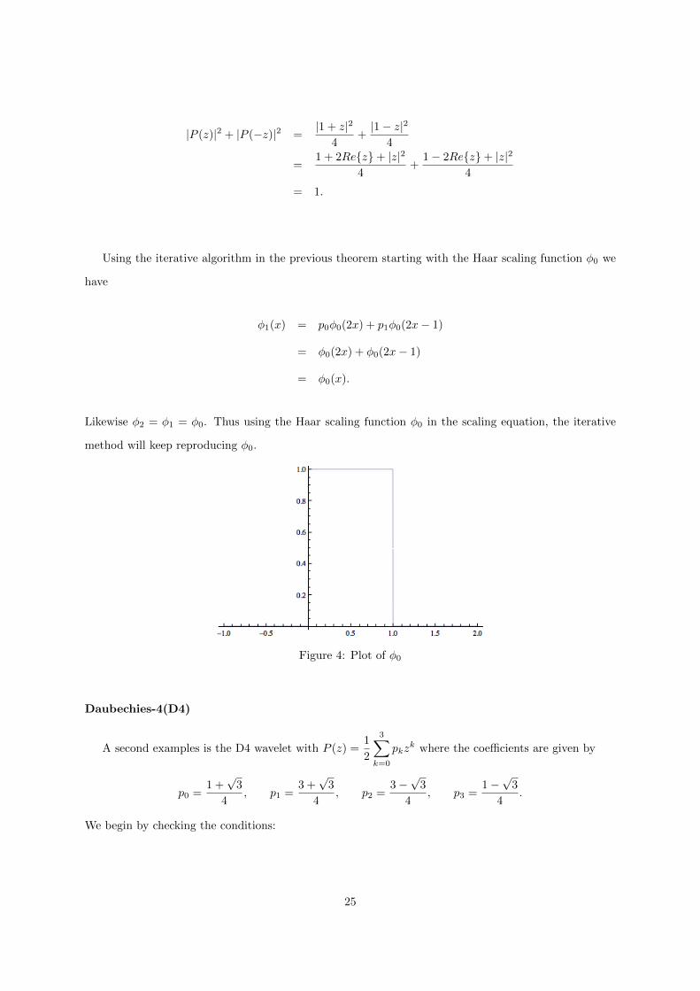
|P (z)|2 + |P (−z)|2 =|1 + z|2
4+|1− z|2
4
=1 + 2Re{z}+ |z|2
4+
1− 2Re{z}+ |z|24
= 1.
Using the iterative algorithm in the previous theorem starting with the Haar scaling function φ0 we
have
φ1(x) = p0φ0(2x) + p1φ0(2x− 1)
= φ0(2x) + φ0(2x− 1)
= φ0(x).
Likewise φ2 = φ1 = φ0. Thus using the Haar scaling function φ0 in the scaling equation, the iterative
method will keep reproducing φ0.
Figure 4: Plot of φ0
Daubechies-4(D4)
A second examples is the D4 wavelet with P (z) =1
2
3∑k=0
pkzk where the coefficients are given by
p0 =1 +√
3
4, p1 =
3 +√
3
4, p2 =
3−√
3
4, p3 =
1−√
3
4.
We begin by checking the conditions:
25

P (1) =1
2
(1 +√
3
4+
3 +√
3
4+
3−√
3
4+
1−√
3
4
)= 1.
We then use an inductive process to obtain φ1 from the coefficients pk and the scaling function φ0.
Computing we get
φ1(x) =
3∑k=0
pkφ0(2x− k)
= p0φ0(2x) + p1φ0(2x− 1) + p2φ0(2x− 2) + p3φ0(2x− 3)
=1 +√
3
4φ0(2x) +
3 +√
3
4φ0(2x− 1) +
3−√
3
4φ0(2x− 2) +
1−√
3
4φ0(2x− 3).
We could then compute φ2, φ3, φ4, ... in a recursive matter. We plot the first few iterations of
φ1, φ2, φ4, φ6 below. The more times we apply the inductive algorithm, the closer we get to the lim-
iting function, φ, which is the D4 scaling function.
Figure 5: Plot of φ1
Figure 6: Plot of φ2
Figure 7: Plot of φ4 Figure 8: Plot of φ6
26
4 Factoring Wavelet Transformations
4.1 Lifting
We denote a vector x of length n by
x = (x[0], x[1], x[2], . . . , x[N − 1]).
We change the notation to x[n] instead of xn to emphasize that a signal can be thought of as a
function of the parameter n. We recall the condition for an infinite signal to have finite energy being
∞∑n=−∞
[x[n]]2 <∞.
Notice that all finite signals will satisfy the above condition and will have finite energy. Before defining
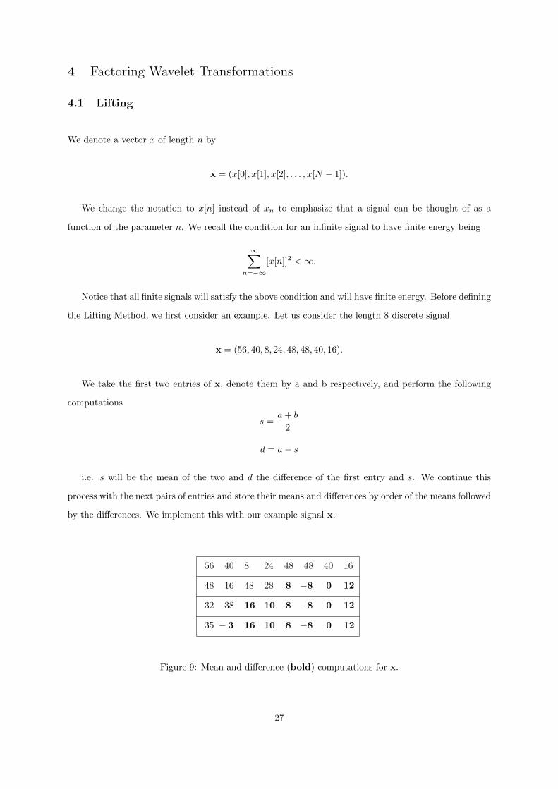
the Lifting Method, we first consider an example. Let us consider the length 8 discrete signal
x = (56, 40, 8, 24, 48, 48, 40, 16).
We take the first two entries of x, denote them by a and b respectively, and perform the following
computations
s =a+ b
2
d = a− s
i.e. s will be the mean of the two and d the difference of the first entry and s. We continue this
process with the next pairs of entries and store their means and differences by order of the means followed
by the differences. We implement this with our example signal x.
56
48
32
35
40
16
38
� 3
8
48
16
16
24
28
10
10
48
8
8
8
48
�8
�8
�8
40
0
0
0
16
12
12
12
1
Figure 9: Mean and difference (bold) computations for x.
27
In the figure above, we have 3 iterations of the lifting method since our signal is of length x = 23.
The first row represents the original signal and the following row represent the 3 iterations of the lifting
method.
It is important to observe that no information has been lost in this transformation of the signal. In
fact, we are able to retrieve the signal by the following inverse computations
a = s+ d
b = s− d.
In Figure 9, for the vector x the first two entries of the third row can be obtained by the last row as
32 = 35 − (−3) and 38 = 35 − (−3). Similarly, the first four entries of the second row using the third
row we have 48 = 32 + 16, 16 = 32−16, 48 = 38 + 10, and 28 = 38−10. The first row is obtained by the
same procedure and thus we have retrieved the original signal x. An important observation to make is
that once we have calculated s, we no longer need the information for b. Also once we calculate d, we no
longer need a. Thus as far as memory is concerned, we can replace the storage of b with s, and a with d.
This transform that uses means and differences brings us to the lifting definition. We can consider the
operations, mean and difference, as specific cases of more general operations. If there is some structure to
the signal, then when taking two samples their difference will most likely be small. In other words, we can
say the first sample is a prediction of the second sample. However, we can use other another prediction
than the one used in the previous example. The other operation we performed with two samples is
computing their mean. It is observed that the pairwise mean values contain the overall structure of the
signal with only half the number of samples. We will refer to this operation as the update process. Similar
to the prediction operation, we can also generalize the update operation to more than just calculating
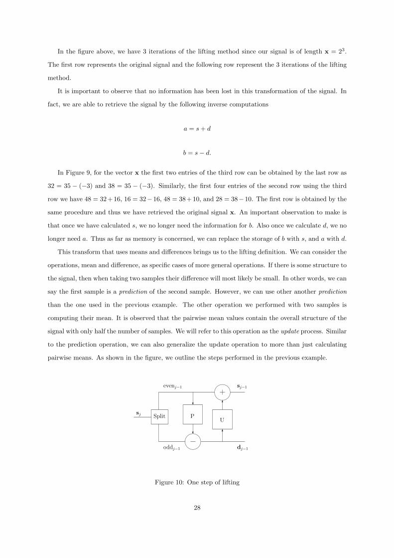
pairwise means. As shown in the figure, we outline the steps performed in the previous example.
oddj�1 dj�1
sj�1
sj Split
evenj�1
?
P
?
���⌧ 6
U
6���⌧
1
Figure 10: One step of lifting
28

Given that we start with a signal sj of length 2j , we first transform the signal to two sequences, each
of length 2j−1, denoted sj−1 and dj−1. We explain the procedure of the figure by the following three
steps:
• Split – The entries of the signal are separated into their even and odd components.
• Prediction – If our signal contains some structure, we are able to have a prediction of the odd
sample based on knowing some information of the even samples. We then replace the odd entry
by the correction to the prediction which we noted as the difference in our previous example.
Therefore, our prediction step is forming the vector d by the following computation
dj−1 = oddj−1 − P (evenj−1).
Thus, our transformed signal is composed of an odd sample minus a prediction based on the number
of even samples.
• Update – We next update our even entry to reflect our knowledge of the signal after performing
the prediction step. In our example, we had a the pairwise average as our update step. In general,
our update step is based on an even entry plus an update based on the know difference detail. We
form the vector s as follows
sj−1 = evenj−1 + U(dj−1).
Here we have performed one iteration of a lifting step. As noted above, if we start with a signal of
length 2j and repeat the lifting step we are allowed to compute up to a j number of times. Our result
would be the stored differences from each lifting step dj,dj−1, ...,d0 and a single number s0[0], which is
the mean value of all the entries from our original signal. The figure below illustrates two steps of lifting.
oddj�1 dj�1
sj�1
sj Split
evenj�1
?
P
?
���⌧ 6
U
6���⌧
Split
oddj�2
evenj�2
���⌧
?
P
? 6
6���⌧
U
dj�2
sj�2
1
Figure 11: Two lifting steps
29

We next introduce the Z-transform of a signal. We can think of this similar to the Fourier transform,
but for a discrete signal. The Z-transform takes a signal from the time domain into the frequency
domain. Since we will be working with Finite Impulse Response (FIR) filters, we say a filter h is a (FIR)
filter if only a finite number of the filter coefficients are non-zero.
Definition 3.1 The Z-transform of a sequence (xk) ∈ `2 is given by
x(z) =∑k
xkz−k.
We can split the signal x(z) to the components even(xe) and odd(xo).
x(z) =∑k
x2kz−2k +
∑k
x2k+1z−(2k+1)
=∑k
x2k(z2)−k + z−1∑k
x2k+1(z2)−k
= xe(z2) + z−1xo(z
2).
More generally, we can then write the even and odd components as:
xe(z) =∑k∈Z
x2kz−k xo(z) =
∑k∈Z
x2k+1z−k.
Similarly, we are able to get the even and odd components from the Z-transform as follows:
xe(z2) =
x(z) + x(−z)2
xo(z2) =
x(z)− x(−z)2z−1
.
4.2 Laurent Polynomials
A Laurent polynomial is an extension of the regular polynomials over a certain field with exponents
allowed to be any integer. If h is a (FIR) filter, then it follows that the Z-transform of h is a Laurent
polynomial of the form
h(z) =
b∑k=a
hkz−k, a ≤ b a, b ∈ Z
where the degree of the Laurent polynomial is defined by
deg h = |h| = b− a.
Note a key difference. As a regular polynomial, zn, has degree n, while as a Laurent polynomial it
30

has degree 0. The Laurent polynomials form a commutative ring denoted by R[z, z−1]. We have that
the sum or difference of two Laurent polynomials is a Laurent polynomial. The product of two Laurent
polynomials with degree l and l′ respectively is also a Laurent polynomial with degree l + l′.
We apply the Division Algorithm for our (FIR) filters. Thus, if we have two Laurent polynomials
a(z) and b(z) 6= 0, then there exists Laurent polynomials q(z)(the quotient) and r(z)(the remainder)
with |r(z)| < |b(z)| such that
a(z) = b(z)q(z) + r(z).
Since the multiplicative identity in R[z, z−1] is 1, we say h 6≡ 0 is a unit if and only if h has a
multiplicative inverse. Equivalently, if h has a multiplicative identity then it has degree 0, which are the
monomials for our ring R[z, z−1]. In other words, we have h−1(z) = 1C z−k, where C ∈ R.
Since a Laurent polynomial is invertible if and only if it is a monomial, then in the ring R[z, z−1]
we have non-uniqueness for the division of two Laurent polynomials. We illustrate this idea with the
following example.
Consider that we want to divide the Laurent polynomial a(z) = −z−1 + 5 − z by b(z) = 2z−1 + 2.
Thus, we need a Laurent polynomial q(z) of degree 1 so that a Laurent polynomial r(z) given by
r(z) = a(z)− b(z)q(z)
is of degree zero. Here is were we have non-uniqueness. Our first choice of q(z) = − 12 + 3z gives us
r(z) = (−z−1 + 5 + z)− (2z−1 + 2)(−1
2+ 3z) = −5z
where the remainder is of degree zero. The second choice of q(z) = − 12 + 1
2z yields
r(z) = (−z−1 + 5 + z)− (2z−1 + 2)(−1
2+
1
2z) = 5
where we again result in reminder of degree zero. The last choice of q(z) = 2 + 3z results in
r(z) = (−z−1 + 5 + z)− (2z−1 + 2)(2 +1
2z) = −5z−1
with the remainder of degree zero.
The result of the Division Algorithm not being unique will be useful for our factorization. In fact,
we will always be able to compute the Division Algorithm and choose the remainder of degree zero to
31

be the constant term.
We will work with the ring of matrices Mat(2× 2,R[z, z−1]) whose elements are of the form
a(z) b(z)
c(z) d(z)
, a, b, c, d ∈ R[z, z−1]
We state the perfect reconstruction conditions for filters h, g, h = g, and g = h in terms of their
Z-transforms
h(z)h(z−1) + g(z)g(z−1) = 2
h(z)h(−z−1) + g(z)g(−z−1) = 0
We define the modulation matrix M(z) as
M(z) =
h(z) h(−z)
g(z) g(−z)
Similarly, we define the dual modulation matrix M(z) as
M(z) =
h(z) h(−z)
g(z) g(−z)
.The perfect reconstruction conditions can now be stated as
M(z−1)TM(z) = 2I
where I is the 2× 2 identity matrix. If all our entries are FIR filters, then the matrices M(z) and M(z)
belong to GL(2× 2,R[z, z−1]), the set of invertible 2× 2 matrices.
4.3 Polyphase Representation
The polyphase matrix, P (z), of a FIR filter pair (h, g) and their conjugates (h, g) is
P (z) =
he(z) ge(z)
ho(z) go(z)
32

where P (z) is similarly defined as
P (z) =
he(z) ge(z)
ho(z) go(z)
.
Note we can rewrite our polyphase matrix using the following identity: P (z2)T =1
2M(z)
1 z
1 −z
.
We prove the following identity below
1
2M(z)
1 z
1 −z
=1
2
h(z) h(−z)
g(z) g(−z)
1 z
1 −z
=
h(z)+h(−z)2zh(z)−zh(−z)
2
g(z)+g(−z)2
zg(z)−zg(−z)2
=
h(z)+h(−z)2h(z)−h(−z)
2z−1
g(z)+g(−z)2
g(z)−g(−z)2z−1
= P (z2)T
Using the previous identity, we are now able to restate our perfect reconstruction condition as shown
in the next theorem due to the work of Daubechies [2].
Theorem 12. We now use the identity, P (z2)T =1
2M(z)
1 z
1 −z
, to restate our perfect reconstruction
condition as
P (z)P (z−1)T = I.
Proof. Using the identity P (z2)T =1
2M(z)
1 z
1 −z
, we have
P (z)P (z−1)T =
1
2M(z)
1 z
1 −z
T 1
2M(z−1)
1 z−1
1 −z−1
=
1
2
1 z
1 −z
T
M(z)T
1
2M(z−1)
1 z−1
1 −z−1
=
1
2
1 z
1 −z
T(1
2M(z)T M(z−1)
)1 z−1
1 −z−1
33
=
1
2
1 z
1 −z
T (I)
1 z−1
1 −z−1
=1
2
1 1
z −z
1 z−1
1 −z−1
=
1
2
2 0
0 2
= I
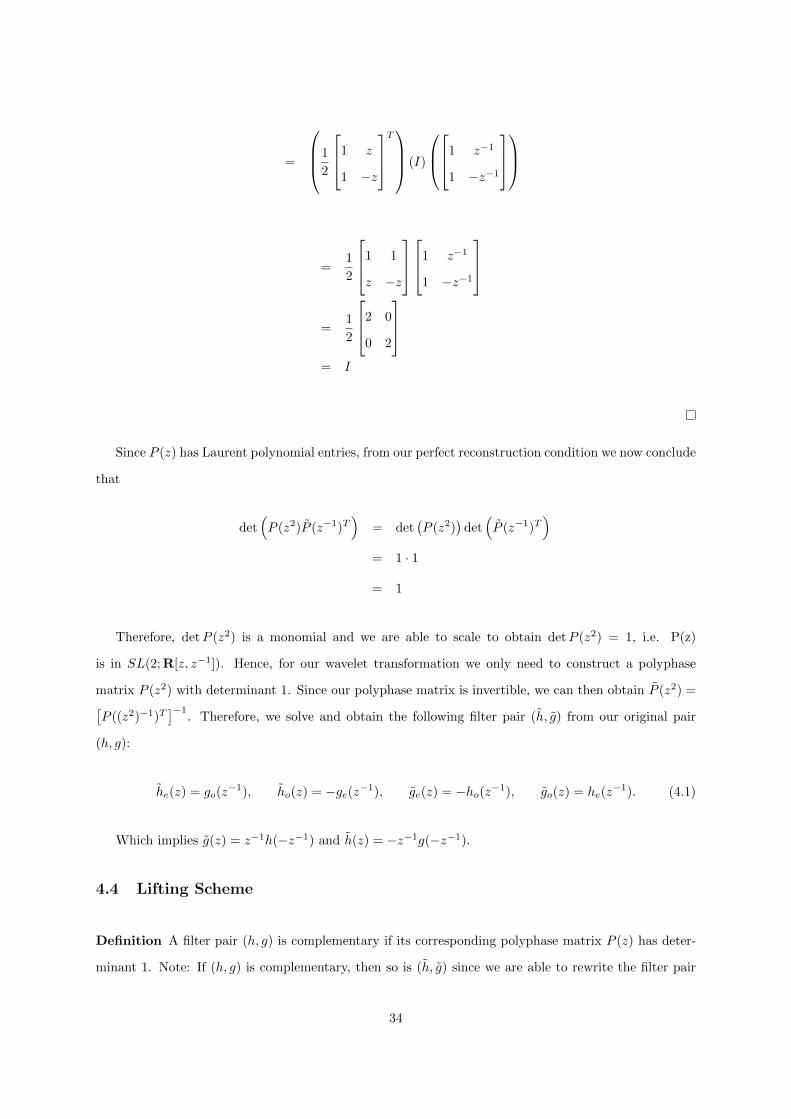
Since P (z) has Laurent polynomial entries, from our perfect reconstruction condition we now conclude
that
det(P (z2)P (z−1)T
)= det
(P (z2)
)det(P (z−1)T
)= 1 · 1
= 1
Therefore, detP (z2) is a monomial and we are able to scale to obtain detP (z2) = 1, i.e. P(z)
is in SL(2; R[z, z−1]). Hence, for our wavelet transformation we only need to construct a polyphase
matrix P (z2) with determinant 1. Since our polyphase matrix is invertible, we can then obtain P (z2) =[P ((z2)−1)T
]−1. Therefore, we solve and obtain the following filter pair (h, g) from our original pair
(h, g):
he(z) = go(z−1), ho(z) = −ge(z−1), ge(z) = −ho(z−1), go(z) = he(z
−1). (4.1)
Which implies g(z) = z−1h(−z−1) and h(z) = −z−1g(−z−1).
4.4 Lifting Scheme
Definition A filter pair (h, g) is complementary if its corresponding polyphase matrix P (z) has deter-
minant 1. Note: If (h, g) is complementary, then so is (h, g) since we are able to rewrite the filter pair
34

(h, g) using (4.1).
Now that we have stated the definition of a complementary filter, in the next two theorems we follow
the approach of Daubechies [2] and obtain the prediction and update steps for our filters in terms of the
polyphase matrix.
Theorem 13. (Primal Lifting) Let (h, g) be complementary, then any other filter g∗ complementary to
h is of the form:
g∗(z) = g(z) + h(z)s(z2)
where s(z2) is a Laurent polynomial.
Proof. Since we can decompose g∗(z) into its even and odd components, we obtain
g∗(z) = g(z) + h(z)s(z2)
=(ge(z
2) + z−1go(z2))
+(he(z
2) + z−1ho(z2))s(z2)
=(ge(z
2) + he(z2)s(z2)
)+ z−1
(go(z
2) + ho(z2)s(z2)
)= g∗e(z2) + z−1g∗o(z2).
So for our filter pair (h, g∗), the polyphase matrix P ∗(z) can be expressed as
P ∗(z) =
he(z) g∗e(z)
ho(z) g∗o(z)
=
he(z) ge(z2) + he(z
2)s(z2)
ho(z) go(z2) + ho(z
2)s(z2)
=
he(z) ge(z)
ho(z) go(z)
1 s(z)
0 1
= P (z)
1 s(z)
0 1
.The determinant of P ∗(z) is 1 since
detP ∗(z) = detP (z) · det
1 s(z)
0 1
= 1 · 1 = 1.
35

The dual polyphase matrix P ∗(z) is then
P ∗(z) =[P ∗(z−1)T
]−1=
1 s(z−1)
0 1
T
P (z−1)T
−1
=[P (z−1)T
]−1 1 0
s(z−1) 1
−1
= P (z)
1 0
−s(z−1) 1
−1
.
So we obtain a new filter pair (h∗, g) where
h∗(z) = h(z)− g(z)s((z2)−1.
Theorem 14. (Dual Lifting)
Let (h, g) be complementary. Then any other filter h∗ complementary to g is of the form:
h∗(z) = h(z) + g(z)t(z2)
where t(z2) is a Laurent polynomial.
Proof. Similarly to Theorem 1, after dual lifting we get the new polyphase matrix
P ∗(z) = P (z)
1 0
t(z) 1
.Dual lifting also creates a new filter g∗(z) given by
g∗(z) = g(z)− h(z)t((z2)−1).
36

4.5 The Euclidean Algorithm
Recall, that the Laurent polynomials form a commutative ring denoted by R[z, z−1]. More than a ring,
the commutative ring of Laurent polynomials, R[z, z−1], is a Euclidean domain. Consequently, R[z, z−1]
being a Euclidean domain makes it also a unique factorization domain, meaning that every non-zero
element can be written in an essentially unique way as a product of a unit and prime elements of the
ring. A Euclidean domain is an integral domain endowed with a Euclidean function. In R[z, z−1], we
define the Euclidean function as the degree of a Laurent polynomial h, by
deg h = |h| = b− a.
The Euclidean algorithm was originated to find the greatest common divisor (GCD) between two
natural numbers. Here it is used to find the GCD between two Laurent polynomials. The main difference
in finding the GCD for Laurent polynomials is that is defined up to units. The units in the ring of Laurent
polynomials are the monomials. This is similar for the case of regular polynomials where the GCD is
defined up to a constant. Similar to natural numbers who are relatively prime if their gcd is one, two
Laurent polynomials are relatively prime if their GCD has degree zero (monomial).
Theorem 15. (Euclidean Algorithm for Laurent Polynomials)
Let a(z) and b(z) 6= 0 be two Laurent polynomials with deg a(z) ≥ deg b(z). We let a0(z) = a(z) and
b0(z) = b(z). There exists a Laurent polynomial qi(z) (quotient) with deg qi(z) = deg a(z) − deg b(z)
and starting at i = 0 we compute:
• ai+1(z) = bi(z)
• bi+1(z) = ai(z)− bi(z)qi+1(z).
Then an(z) = gcd(a(z), b(z)) where n is the smallest number for which bn(z) = 0.
Since deg bi+1(z) < deg bi(z), then there is an m for which deg bm(z) = 0. Thus, the algorithm has
a total of n = m+ 1 number of iterations. Therefore, the number of steps is bounded by n ≤ |b(z)|+ 1.
For qi+1(z) = ai(z)/bi(z), we have that
an(z)
0
=
1∏i=n
0 1
1 −qi(z)
a(z)
b(z)
.
37

Therefore, by inverting we obtain
a(z)
b(z)
=
n∏i=1
qi(z) 1
1 0
an(z)
0
.Thus, an(z) divides both a(z) and b(z). If an(z) results in a monomial, then a(z) and b(z) are
relatively prime.
If we take the same example of Laurent polynomials a(z) = a0(z) = −z−1 + 5− z and b(z) = b0(z) =
2z−1 + 2. Then applying the Euclidean algorithm we get
• a1(z) = b0(z) = 2z−1 + 2
• b1(z) = a0(z)− b0(z)q1(z) = (−z−1 + 5− z)− (2z−1 + 2)
(−1
2+
1
2z
)= 5
A second iteration yields
• a2(z) = b1(z) = 5
• b2(z) = a1(z)− b1(z)q2(z) = (2z−1 + 2)− (5)
(2z−1
5+
2
5
)= 0
Thus, the gcd(a(z), b(z)) = 5. Hence, a(z) and b(z) are relatively prime and we have
−z−1 + 5− z
2z−1 + 2
=
−1
2+
1
2z 1
1 0
2z−1
5+
2
51
1 0
5
0
.In this example, the number of iterations was n = 2 = |b(z)|+ 1.
4.6 Factoring Algorithm
We consider a complementary filter pair (h, g) that can be factored into lifting steps. First, note that
the polyphase components he(z) and h0(z) must be relatively prime, if not we would have a common
factor in our detP (z) which must be 1. We can then run the Euclidean algorithm on he(z) and h0(z)
and obtain a gcd of a monomial. Since the division is not unique, we can choose to have the GCD to be
a monomial which is a constant. We will call this constant K and follow the ideas of Daubechies [2] to
obtain he(z)h0(z)
=
n∏i=1
qi(z) 1
1 0
K
0
.A special case if |he(z)| > |h0(z)|, then we can simply choose q1(z) = 0. Otherwise we can assume
the n to always be even, because if n is odd we multiply h(z) by z and g(z) by z−1. The detP (z) is still
38
1 by a simple calculation. Given a filter h we can find a complementary filter g∗ by letting
P ∗(z) =
he(z) g∗e(z)
h0(z) g∗0(z)
=
n∏i=1
qi(z) 1
1 0
K 0
0 1/K
.where detP ∗(z) = 1 since n is even it follows
detP ∗(z) = det
n∏i=1
qi(z) 1
1 0
K 0
0 1/K
= (−1)n(1) = 1.
We make the observation that the first matrix in our product can be rewritten as follows
qi(z) 1
1 0
=
1 qi(z)
0 1
0 1
1 0
=
0 1
1 0
1 0
qi(z) 1
. (4.2)
Using the first form of (4.2) when i is odd and the second form when i is even we can rewrite P ∗(z)
as follows
P ∗(z) =
n/2∏i=1
1 q2i−1(z)
0 1
0 1
1 0
0 1
1 0
1 0
q2i(z) 1
K 0
0 1/K
=
n/2∏i=1
1 q2i−1(z)
0 1
1 0
q2i(z) 1
K 0
0 1/K
(4.3)
Now we are able to recover the filter g from g∗ by the lifting scheme below
P (z) = P ∗(z)
1 s(z)
0 1
(4.4)
Theorem 16. Given a complementary filter pair (h, g), then there exists Laurent polynomials si(z) and
ti(z) for 1 ≤ i ≤ m and a nonzero constant K so that
P (z) =
m∏i=1
1 si(z)
0 1
1 0
ti(z) 1
K 0
0 1/K
.We can prove the theorem by combining the previous results in equation (4.3) and (4.4). Last, define
m = n/2 + 1 for tm(z) = 0 and s(z) = K2s(z). In other words, we have that every finite filter wavelet
transform can be factored into m lifting steps followed by a scaling.
39

The dual polyphase matrix P (z) is then given as
P (z) =
m∏i=1
1 0
−s(z−1) 1
1 −t(z−1)
0 1
1/K 0
0 K
.4.7 Examples
From Daubechies [2], we confirm the factorizations of the following wavelet transformations.
(Haar Wavelet)
We consider the Haar filter pair (normalized) given by h(z) = 1 + z−1 , g(z) = −1/2 + 1/2z−1 ,
h(z) = 1/2 + 1/2z−1 , and g(z) = −1 + z−1. Therefore, our polyphase matrix P (z) is the following
P (z) =
1 −1/2
1 1/2
= P ∗(z)
1 s(z)
0 1
=
he(z) = 1 g∗e(z)
ho(z) = 1 g∗o(z)
1 s(z)
0 1
=
1 0
1 1
1 −1/2
0 1
where the last equation comes from solving for g∗e(z) and g∗o(z) by the following system
−1/2 = s(z) + g∗e(z)
1/2 = s(z) + g∗o(z).
Letting s(z) = 1/2 we solve and get g∗e(z) = 0 and g∗o(z) = 1. Thus, our polyphase matrix P (z) for
the Haar can be factored into the following form
P (z) =
1 0
1 1
1 −1/2
0 1
.
40

This factorization corresponds to the following forward transform using lifting steps:
s(0)l = x2l
d(0)l = x2l+1
dl = d(0)l − s
(0)l
sl = s(0)l + 1/2dl.
Using our perfect reconstruction condition (), we solve for P (z) and get
P (z) = P (z−1)
= P (z)−1
=
1 0
1 1
1 −1/2
0 1
−1
=
1 1/2
0 1
1 0
−1 1
where we used the fact that P (z) = P (z−1) in the first equation. This leads to the following lifting steps
for the inverse transform:
s(0)l = sl − 1/2dl
d(0)l = dl + s
(0)l
x2l+1 = d(0)l
x2l = s(0)l .
Daubechies-4 (D4)
For the (D4) our filters of h and g are given by:
h(z) = h0 + h1z−1 + h2z
−2 + h3z−3
g(z) = −h3z2 + h2z − h1 + h0z−1
where the coefficients are given by
h0 =1 +√
3
4√
2, h1 =
3 +√
3
4√
2, h2 =
3−√
3
4√
2, h3 =
1−√
3
4√
2.
41

We notice that for the D4 we have P (z) = P (z), thus the polyphase matrix is given by
P (z) =
h0 + h2z−1 −h3z − h1
h1 + h3z−1 h2z + h0
=
1+√3
4√2
+ 3−√3
4√2z−1 − 1−
√3
4√2− 3+
√3
4√2
3+√3
4√2
+ 1−√3
4√2z−1 3−
√3
4√2z + 1+
√3
4√2
.Applying the Euclidean algorithm, we get
a1 = b0 = 3+√3
4√2
+ 1−√3
4√2z−1
b1 = a0 − b0q1= 1+
√3
4√2
3−√3
4√2z−1 −
(3+√3
4√2
+ 1−√3
4√2z−1)
(−√
3)
= 1+√3+3√3+3
4√2
= 1+√3√
2
a2 = b1 = 1+√3
2
b2 = a1 − b1q2= 3+
√3
4√2
+ 1−√3
4√2z−1 −
(1+√3√
2
)(√34 +
√3−24 z−1
)= 3+
√3
4√2− 3+
√3
4√2
+ 1−√3
4√2z−1 − 3−2+3−2
√3
4√2
z−1
= 0.
Therefore, our gcd = b1 = 1+√3
2 and our factorization is the following
P (z) =
1 −√
3
0 1
1 0√34 +
√3−24 z−1 1
1 z
0 1
√3+1√2
0
0√3−1√2
.Since our polyphase matrix is unitary, we use the fact that P (z) = P (z) and obtain one form of
factorization as
P (z−1)T =
√3+1√2
0
0√3−1√2
1 0
z−1 1
1
√34 +
√3−24 z
0 1
1 0
−√
3 1
.
42

Thus in terms of lifting steps we get the following for the forward transform:
d(1)l = x2l+1 −
√3x2l
s(1)l = x2l +
√3/4d
(1)l + (
√3− 2)/4d
(1)l+1
d2l = d(1)l + s
(1)l−1
sl = (√
3 + 1)/√
2s(1)l
dl = (√
3− 1)/√
2d(2)l .
Where the inverse transform is obtained from inverting our lifting steps:
d(2)l = (
√3 + 1)/
√2dl
s(1)l = (
√3− 1)/
√2sl
d1l = d(2)l − s
(1)l−1
x2l = s(1)l −
√3/4d
(1)l − (
√3− 2)/4d
(1)l+1
x2l+1 = d(1)l +
√3x2l.
Our second form of factorization comes from the fact that P (z)−1 = P (z−1)T and use equation () to
get the factorization as
P (z)−1 =
√3−1√2
0
0√3+1√2
1 −z
0 1
1 0
−√34 −
√3−24 z−1 1
1
√3
0 1
.which leads to the forward transform lifting steps:
s(1)l = x2l +
√3x2l+1
d(1)l = x2l+1 −
√3/4s
(1)l − (
√3− 2)/4s
(1)l−1
s2l = s(1)l − d
(1)l+1
sl = (√
3− 1)/√
2s(1)l
dl = (√
3 + 1)/√
2d(2)l
Where the inverse transform is obtained from inverting our lifting steps:
d(2)l = (
√3− 1)/
√2dl
s(1)l = (
√3 + 1)/
√2sl
d1l = d(2)l + s
(1)l−1
x2l = s(1)l +
√3/4d
(1)l + (
√3− 2)/4d
(1)l+1
x2l+1 = d(1)l −
√3x2l.
43

Cohen-Daubechies-Feauveau 5-3 CDF(5,3)
The next filter we introduce is know as the LeGall filter pair which is used for the JPEG-2000 lossless
compression algorithm Van Fleet [8]. For the CDF(5, 3), the filter h is symmetric and given by:
h(z) = h2z−2 + h1z
−1 + h0 + h1z + h2z2
where the coefficients are given by
h0 =3
4, h1 =
1
4, h2 = −1
8.
Applying the Euclidean algorithm and letting a0 = − 18z−2 + 3
4 − 18z
2 and b0 = 14z−1 + 1
4z, we obtain
a1 = b0 = 14z−1 + 1
4z
b1 = a0 − b0q1=
(− 1
8z−2 + 3
4 − 18z
2)−(14z−1 + 1
4z) (− 1
2 (z−1 + z))
= 1
a2 = b1 = 1
b2 = a1 − b1q2=
(14z−1 + 1
4z)− (1)
(14 (z−1 + z)
)= 0.
Therefore, our gcd = b1 = 1 and our factorization is the following
P (z) =
1 − 12 (z−1 + z)
0 1
1 0
14 (z−1 + z) 1
1 0
0 1/1
=
1 − 12 (z−1 + z)
0 1
1 0
14 (z−1 + z) 1
.Hence, in terms of lifting steps we get the following for the forward transform:
s(0)l = x2l
d(0)l = x2l+1
d(1)l = s
(0)l − 1
2 (d(0)l + d
(0)l−1)
s(1)l = d
(0)l + 1
4 (s(0)l + s
(0)l−1)
sl = (1)s(1)l
dl = (1/1)d(2)l
Note we will be able to omit the last two lifting steps since our gcd = 1 for this filter.
44

Daubechies-6 (D6)
For our next example we have the Daubechies-6 which is of length 6 where the low pass filter is given
by the Laurent polynomial
h(z) =
3∑k=−2
hkz−k
where the coefficients are
h−2 =
√2(1 +
√10 +
√5 + 2
√10)
32h−1 =
√2(5 +
√10 + 3
√5 + 2
√10)
32
h0 =
√2(10− 2
√10 + 2
√5 + 2
√10)
32h1 =
√2(10− 2
√10− 2
√5 + 2
√10)
32
h2 =
√2(5 +
√10− 3
√5 + 2
√10)
32h3 =
√2(1 +
√10− 5
√5 + 2
√10)
32.
The polyphase components for the (D6) are
he(z) = h−2z + h0 + h2z−1 ge(z) = −h3z − h1 − h−1z−1
h0(z) = h−1z + h1 + h3z−1 g0(z) = h2z + h0 + h−2z
−1.
The factorization is then given by:
P (z) =
1 0
α 1
1 βz−1 + β′
0 1
1 0
γ + γ′z 1
1 δ
0 1
ξ 0
0 1ξ
where the coefficients are
α = −0.4122865950
β = −1.5651362796
β′ = 0.3523876576
γ = 0.0284590896
γ′ = 0.4921518449
δ = −0.3896203900
ξ = 1.9182029462.
45

This leads to the forward transform lifting steps:
s(1)l = x2l + αx2l+1
d(1)l = x2l+1 + βs
(1)l−1 + β′s
(1)l
s(2)l = s
(1)l + γd
(1)l + γ′d
(1)l+1
d(2)l = d
(1)l + δs2l
sl = ξs(2)l
dl = d(2)l /ξ
Where the inverse transform is obtained from inverting our lifting steps:
d(2)l = dlξ
s(2)l = sl/ξ
d(1)l = d
(2)l − δs
(2)l
s(1)l = s
(2)l − γd
(1)l − γ′d
(1)l+1
x2l+1 = d(1)l − βs
(1)l−1 − β′s
(1)l
x2l = s(1)l − αx2l+1.
Cohen-Daubechies-Feauveau 9-7 (CDF(9,7))
Here we consider the popular filter pair used in the JPEG 2000 algorithm. Here we have a biorthogonal
symmetric filter pairs. The lowpass filters h and h each have 9 and 7 coefficients respectively and similarly
for the high pass filter pair g and g. We consider the following polyphase components for the forward
transform:
he(z) = h4(z2 + z−2) + h2(z + z−1) + h0, ho(z) = h3(z2 + z−1) + h1(z + 1).
The factorization is then given by:
P (z) =
1 α(1 + z−1)
0 1
1 0
β(1 + z) 1
1 γ(1 + z−1)
0 1
1 0
δ(1 + z) 1
ξ 0
0 1ξ
46
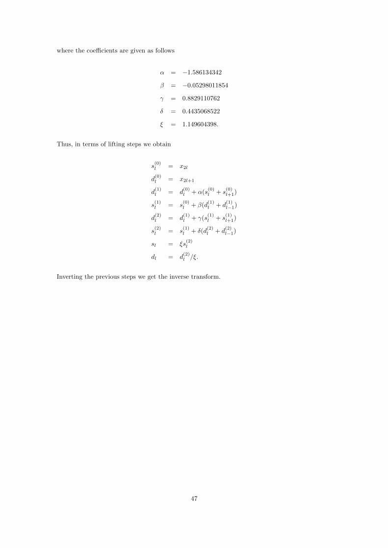
where the coefficients are given as follows
α = −1.586134342
β = −0.05298011854
γ = 0.8829110762
δ = 0.4435068522
ξ = 1.149604398.
Thus, in terms of lifting steps we obtain
s(0)l = x2l
d(0)l = x2l+1
d(1)l = d
(0)l + α(s
(0)l + s
(0)l+1)
s(1)l = s
(0)l + β(d
(1)l + d
(1)l−1)
d(2)l = d
(1)l + γ(s
(1)l + s
(1)l+1)
s(2)l = s
(1)l + δ(d
(2)l + d
(2)l−1)
sl = ξs(2)l
dl = d(2)l /ξ.
Inverting the previous steps we get the inverse transform.
47

5 Conclusion and Remarks
We conclude with the comparison of the lifting method resulting in fewer computations than the standard
wavelet transform as is done in Daubechies [2]. The standard wavelet transform will be referred to as
applying the polyphase matrix P (z) to the filter h as shown below
P (z)
he(z)
z−1ho(z)
.Notice that in either method we will have subsampled and we can compare the computations. The
unit we will use to compare the two algorithms is cost. Cost of computing either algorithm is based on
the number of multiplications and additions. For a filter h, the cost of applying the standard algorithm
to a filter h is |h| + 1 multiplications and |h| additions. The cost of the standard algorithm is then
2(|h|+ |g|) + 2. We see this for our example of the D4. The filters h and g for our D4 are given as
h(z) = h0 + h1z−1 + h2z
−2 + h3z−3
g(z) = −h3z2 + h2z − h1 + h0z−1.
Therefore, for h we have |h| = 3 and for g we have |g| = 3. Hence, the cost of implementing the
standard algorithm for our D4 is
2(|h|+ |g|) + 2 = 2(3 + 3) + 2 = 14.
If the filter h is symmetric and |h| is even, then the cost of applying the standard algorithm 3|h|/2+1.
As we saw in our examples, the CDF(9,7) was a symmetric filter with |h| = 8 and |g| = 6. Thus, the
cost of implementing the CDF(9,7) through the standard algorithm is
(3|h|
2+ 1
)+
(3|g|2
+ 1
)=
3(8)
2+ 1 +
3(6)
2+ 1 = 23.
We consider a more general case with non-symmetric filters. Let |h| = 2N and |g| = 2M . The cost
using the standard algorithm is then
2(|h|+ |g|) + 2 = 2(2N + 2M) + 2 = 4(N +M) + 2.
For the cost using the lifting method, we have that the polyphase components will have |he| =
N, |ho| = N − 1, |ge| = M, and |go| = M − 1. When we compute the Euclidean algorithm for the a filter
48
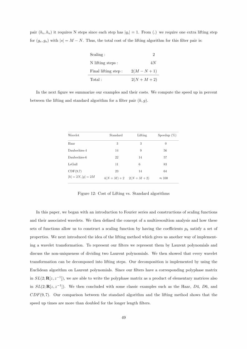
pair (he, ho) it requires N steps since each step has |qi| = 1. From (.) we require one extra lifting step
for (ge, go) with |s| = M −N . Thus, the total cost of the lifting algorithm for this filter pair is:
Scaling : 2
N lifting steps : 4N
Final lifting step : 2(M −N + 1)
Total : 2(N +M + 2)
In the next figure we summarize our examples and their costs. We compute the speed up in percent
between the lifting and standard algorithm for a filter pair (h, g).
Wavelet Standard Lifting Speedup (%)
Haar
Daubechies-4
Daubechies-6
LeGall
CDF(9,7)
|h| = 2N, |g| = 2M
3
14
22
11
23
4(N + M) + 2
3
9
14
6
14
2(N + M + 2)
0
56
57
83
64
⇡ 100
1
Figure 12: Cost of Lifting vs. Standard algorithms
In this paper, we began with an introduction to Fourier series and constructions of scaling functions
and their associated wavelets. We then defined the concept of a multiresoultion analysis and how these
sets of functions allow us to construct a scaling function by having the coefficients pk satisfy a set of
properties. We next introduced the idea of the lifting method which gives us another way of implement-
ing a wavelet transformation. To represent our filters we represent them by Laurent polynomials and
discuss the non-uniqueness of dividing two Laurent polynomials. We then showed that every wavelet
transformation can be decomposed into lifting steps. Our decomposition is implemented by using the
Euclidean algorithm on Laurent polynomials. Since our filters have a corresponding polyphase matrix
in SL(2; R[z, z−1]), we are able to write the polyphase matrix as a product of elementary matrices also
in SL(2; R[z, z−1]). We then concluded with some classic examples such as the Haar, D4, D6, and
CDF (9, 7). Our comparison between the standard algorithm and the lifting method shows that the
speed up times are more than doubled for the longer length filters.
49

References
[1 ] A. Boggess and F.J. Narcowich. A First Course in Wavelets with Fourier Analysis. Prentice
Hall, Upper Saddle River, NJ, 2001.
[2 ] I. Daubechies and W. Sweldens. ”Factoring Wavelet Transformations into Lifting Steps”. Fourier
Analysis and Applications. 4:3 (1998), 247-269.
[3 ] A. Deitmar. A First Course in Harmonic Analysis. Springer-Verlag, New York, NY, 2005.
[4 ] A. Jensen and A. la Cour-Harbo. Ripples in Mathematics: The Discrete Wavelet Transform.
Springer-Verlag, Berlin 2001.
[5 ] H.L. Royden and P.M. Fitzpatrick. Real Analysis. Prentice Hall, Boston, MA, 2010.
[6 ] D.K. Ruch and P.J. Van Fleet. Wavelet Theory: An Elementary Approach with Applications.
Wiley-Interscience, Hoboken, NJ, 2009.
[7 ] W. Rudin. Real and Complex Analysis. McGraw-Hill, 1987.
[8 ] P.J. Van Fleet. Discrete Wavelet Transformations: An Elementary Approach with Applications.
Wiley-Interscience, Hoboken, NJ, 2008.
50

Appendix
The appendix contains the code for the factorization of the wavelet transformation through both the
standard and lifting method. We used the software Mathematica for all the implementations. The first
we display is the Haar lowpass, h, and the high pass, g, filters with the coefficients multiplied by a
normalizing factor of 1√2. We then display the 8 × 8 matrix used for implementing the Haar wavelet
transform.
Haar (D2)In[573]:= h0 = 1 ê Sqrt@2D
h1 = 1 ê Sqrt@2Dg0 = 1 ê Sqrt@2Dg1 = -1 ê Sqrt@2D
Out[573]=1
2
Out[574]=1
2
Out[575]=1
2
Out[576]= -1
2
In[577]:= H1@n_D := Module@8h0 = 1 ê Sqrt@2D, h1 = 1 ê Sqrt@2D,h2 = 1, g0 = 1 ê Sqrt@2D, g1 = -1 ê Sqrt@2D<, Join@SparseArray@88i_, j_< ê; j == 2 i -> h0, 8i_, j_< ê; j == 2 i - 1 -> h1<, 8n ê 2, n<D,SparseArray@88i_, j_< ê; j == 2 i Æ g1, 8i_, j_< ê; j == 2 i - 1 Æ g0<, 8n ê 2, n<DDD
MatrixForm@H1@8DDOut[578]//MatrixForm=
1
2
1
20 0 0 0 0 0
0 0 1
2
1
20 0 0 0
0 0 0 0 1
2
1
20 0
0 0 0 0 0 0 1
2
1
21
2- 1
20 0 0 0 0 0
0 0 1
2- 1
20 0 0 0
0 0 0 0 1
2- 1
20 0
0 0 0 0 0 0 1
2- 1
2
Here we check that the reconstruction conditions hold for our Haar wavelet transformation matrix and
its transpose.
In[579]:= MatrixForm@[email protected]@H1@8DDDOut[579]//MatrixForm=
1 0 0 0 0 0 0 00 1 0 0 0 0 0 00 0 1 0 0 0 0 00 0 0 1 0 0 0 00 0 0 0 1 0 0 00 0 0 0 0 1 0 00 0 0 0 0 0 1 00 0 0 0 0 0 0 1
Example of vector w (3 lifting steps)In[580]:= w = 856, 40, 8, 24, 48, 48, 40, 16<
odd1 = Partition@w, 2D@@All, 1DD;even1 = Partition@w, 2D@@All, 2DD;s1 = Hodd1 + even1L ê 2;d1 = odd1 - s1;w1 = Join@s1, d1Dodd2 = Partition@s1, 2D@@All, 1DD;even2 = Partition@s1, 2D@@All, 2DD;s2 = Hodd2 + even2L ê 2;d2 = odd2 - s2;w2 = Join@s2, d2, d1Dodd3 = Partition@s2, 2D@@All, 1DD;even3 = Partition@s2, 2D@@All, 2DD;s3 = Hodd3 + even3L ê 2;d3 = odd3 - s3;w3 = Join@s3, d3, d2, d1D
Out[580]= 856, 40, 8, 24, 48, 48, 40, 16<Out[585]= 848, 16, 48, 28, 8, -8, 0, 12<Out[590]= 832, 38, 16, 10, 8, -8, 0, 12<Out[595]= 835, -3, 16, 10, 8, -8, 0, 12<
2 Haar.nb
51

We have the implementation of 3 transforms of the Haar to a vector w.
Example of vector w (3 DWT-Haar)In[596]:= a1 = H1 ê Sqrt@2DL * [email protected];
s1 = Take@a1, 4D;d1 = Take@a1, -4D;a2 = H1 ê Sqrt@2DL * [email protected];s2 = Take@a2, 2D;d2 = Take@a2, -2D;a3 = H1 ê Sqrt@2DL * [email protected];s3 = Take@a3, 1D;d3 = Take@a3, -1D;Join@s3, d3, d2, d1D
Out[605]= 835, -3, 16, 10, 8, -8, 0, 12<
Haar.nb 3
We check our results with the lifting method and we see we get the same through either implemen-
tation. The first row represents the same original vector w as used in the example above. The last three
rows represent three lifting steps and the last row is our transformed vector.
In[579]:= MatrixForm@[email protected]@H1@8DDDOut[579]//MatrixForm=
1 0 0 0 0 0 0 00 1 0 0 0 0 0 00 0 1 0 0 0 0 00 0 0 1 0 0 0 00 0 0 0 1 0 0 00 0 0 0 0 1 0 00 0 0 0 0 0 1 00 0 0 0 0 0 0 1
Example of vector w (3 lifting steps)In[580]:= w = 856, 40, 8, 24, 48, 48, 40, 16<
odd1 = Partition@w, 2D@@All, 1DD;even1 = Partition@w, 2D@@All, 2DD;s1 = Hodd1 + even1L ê 2;d1 = odd1 - s1;w1 = Join@s1, d1Dodd2 = Partition@s1, 2D@@All, 1DD;even2 = Partition@s1, 2D@@All, 2DD;s2 = Hodd2 + even2L ê 2;d2 = odd2 - s2;w2 = Join@s2, d2, d1Dodd3 = Partition@s2, 2D@@All, 1DD;even3 = Partition@s2, 2D@@All, 2DD;s3 = Hodd3 + even3L ê 2;d3 = odd3 - s3;w3 = Join@s3, d3, d2, d1D
Out[580]= 856, 40, 8, 24, 48, 48, 40, 16<Out[585]= 848, 16, 48, 28, 8, -8, 0, 12<Out[590]= 832, 38, 16, 10, 8, -8, 0, 12<Out[595]= 835, -3, 16, 10, 8, -8, 0, 12<
2 Haar.nb
Similarly, we have the code for the D4. We display the coefficients and the wavelet transform matrix.
We also include the lifting implementation to demonstrate the transformed vector for both methods.
52

Daubechies-4 (D4)
In[606]:= h0 = H1 + Sqrt@3DL ê H4 * Sqrt@2DLh1 = H3 + Sqrt@3DL ê H4 * Sqrt@2DLh2 = H3 - Sqrt@3DL ê H4 * Sqrt@2DLh3 = H1 - Sqrt@3DL ê H4 * Sqrt@2DLg0 = h3g1 = -h2g2 = h1g3 = -h0
Out[606]=1 + 3
4 2
Out[607]=3 + 3
4 2
Out[608]=3 - 3
4 2
Out[609]=1 - 3
4 2
Out[610]=1 - 3
4 2
Out[611]= -3 - 3
4 2
Out[612]=3 + 3
4 2
Out[613]= -1 + 3
4 2
In[614]:= D4@n_D := Module@8h0 = H1 + Sqrt@3DL ê H4 * Sqrt@2DL,h1 = H3 + Sqrt@3DL ê H4 * Sqrt@2DL, h2 = H3 - Sqrt@3DL ê H4 * Sqrt@2DL,h3 = H1 - Sqrt@3DL ê H4 * Sqrt@2DL, g0 = h3, g1 = -h2, g2 = h1, g3 = -h0<,
Join@SparseArray@88i_, j_< ê; j == 2 i - 1 -> h0, 8i_, j_< ê; j == 2 i -> h1,8i_, j_< ê; j == 2 i + 1 -> h2, 8i_, j_< ê; j == 2 i + 2 -> h3,8n ê 2, 1< -> h2, 8n ê 2, 2< -> h3<, 8n ê 2, n<D,SparseArray@88i_, j_< ê; j == 2 i - 1 Æ g0, 8i_, j_< ê; j == 2 i Æ g1,8i_, j_< ê; j == 2 i + 1 Æ g2, 8i_, j_< ê; j == 2 i + 2 Æ g3,8n ê 2, 1< Æ g2, 8n ê 2, 2< Æ g3<, 8n ê 2, n<DDD
MatrixForm@D4@8DD
Out[615]//MatrixForm=
1+ 3
4 2
3+ 3
4 2
3- 3
4 2
1- 3
4 20 0 0 0
0 0 1+ 3
4 2
3+ 3
4 2
3- 3
4 2
1- 3
4 20 0
0 0 0 0 1+ 3
4 2
3+ 3
4 2
3- 3
4 2
1- 3
4 2
3- 3
4 2
1- 3
4 20 0 0 0 1+ 3
4 2
3+ 3
4 2
1- 3
4 2- 3- 3
4 2
3+ 3
4 2- 1+ 3
4 20 0 0 0
0 0 1- 3
4 2- 3- 3
4 2
3+ 3
4 2- 1+ 3
4 20 0
0 0 0 0 1- 3
4 2- 3- 3
4 2
3+ 3
4 2- 1+ 3
4 2
3+ 3
4 2- 1+ 3
4 20 0 0 0 1- 3
4 2- 3- 3
4 2
In[616]:= N@Chop@MatrixForm@[email protected]@D4@8DDDDDOut[616]//MatrixForm=
1. 0. 0. 0. 0. 0. 0. 0.0. 1. 0. 0. 0. 0. 0. 0.0. 0. 1. 0. 0. 0. 0. 0.0. 0. 0. 1. 0. 0. 0. 0.0. 0. 0. 0. 1. 0. 0. 0.0. 0. 0. 0. 0. 1. 0. 0.0. 0. 0. 0. 0. 0. 1. 0.0. 0. 0. 0. 0. 0. 0. 1.
2 D4.nb
53

In[614]:= D4@n_D := Module@8h0 = H1 + Sqrt@3DL ê H4 * Sqrt@2DL,h1 = H3 + Sqrt@3DL ê H4 * Sqrt@2DL, h2 = H3 - Sqrt@3DL ê H4 * Sqrt@2DL,h3 = H1 - Sqrt@3DL ê H4 * Sqrt@2DL, g0 = h3, g1 = -h2, g2 = h1, g3 = -h0<,
Join@SparseArray@88i_, j_< ê; j == 2 i - 1 -> h0, 8i_, j_< ê; j == 2 i -> h1,8i_, j_< ê; j == 2 i + 1 -> h2, 8i_, j_< ê; j == 2 i + 2 -> h3,8n ê 2, 1< -> h2, 8n ê 2, 2< -> h3<, 8n ê 2, n<D,SparseArray@88i_, j_< ê; j == 2 i - 1 Æ g0, 8i_, j_< ê; j == 2 i Æ g1,8i_, j_< ê; j == 2 i + 1 Æ g2, 8i_, j_< ê; j == 2 i + 2 Æ g3,8n ê 2, 1< Æ g2, 8n ê 2, 2< Æ g3<, 8n ê 2, n<DDD
MatrixForm@D4@8DD
Out[615]//MatrixForm=
1+ 3
4 2
3+ 3
4 2
3- 3
4 2
1- 3
4 20 0 0 0
0 0 1+ 3
4 2
3+ 3
4 2
3- 3
4 2
1- 3
4 20 0
0 0 0 0 1+ 3
4 2
3+ 3
4 2
3- 3
4 2
1- 3
4 2
3- 3
4 2
1- 3
4 20 0 0 0 1+ 3
4 2
3+ 3
4 2
1- 3
4 2- 3- 3
4 2
3+ 3
4 2- 1+ 3
4 20 0 0 0
0 0 1- 3
4 2- 3- 3
4 2
3+ 3
4 2- 1+ 3
4 20 0
0 0 0 0 1- 3
4 2- 3- 3
4 2
3+ 3
4 2- 1+ 3
4 2
3+ 3
4 2- 1+ 3
4 20 0 0 0 1- 3
4 2- 3- 3
4 2
In[616]:= N@Chop@MatrixForm@[email protected]@D4@8DDDDDOut[616]//MatrixForm=
1. 0. 0. 0. 0. 0. 0. 0.0. 1. 0. 0. 0. 0. 0. 0.0. 0. 1. 0. 0. 0. 0. 0.0. 0. 0. 1. 0. 0. 0. 0.0. 0. 0. 0. 1. 0. 0. 0.0. 0. 0. 0. 0. 1. 0. 0.0. 0. 0. 0. 0. 0. 1. 0.0. 0. 0. 0. 0. 0. 0. 1.
2 D4.nb
Example Via LiftingIn[617]:= w = RandomInteger@8-128, 127<, 816<D
odd1 = Partition@w, 2D@@All, 2DD;even1 = Partition@w, 2D@@All, 1DD;d1 = odd1 - Sqrt@3D * even1;s1 = even1 + HSqrt@3D ê 4L * d1 + HHSqrt@3D - 2L ê 4L * RotateLeft@d1D;d2 = d1 + RotateRight@s1D;s = HHSqrt@3D + 1L ê Sqrt@2DL * s1;d = RotateLeft@HH1 - Sqrt@3DL ê Sqrt@2DL * d2D;Chop@N@Join@s, dDDD
Out[617]= 880, 88, 90, 36, -119, -82, -49, -17, -121, -55, -82, -69, -21, 110, 118, -21<Out[625]= 8127.765, 57.5197, -134.85, -57.8898, -113.897, -116.265, 111.041, 45.9663,
27.8224, -79.6585, 1.0006, -64.504, -7.28343, -44.6153, 86.9129, 13.8573<Example Via D4 Wavelet TransformIn[626]:= Chop@N@[email protected][626]= 8127.765, 57.5197, -134.85, -57.8898, -113.897, -116.265, 111.041, 45.9663,
27.8224, -79.6585, 1.0006, -64.504, -7.28343, -44.6153, 86.9129, 13.8573<
D4.nb 3
The next set of code we have has the CDF(5, 3) wavelet transformation matrices. Notice we have a
biorthogonal pair here. We also demonstrate the example through both the standard and lifting method.
CDF (5,3)In[68]:= LG1@n_D := Module@8h0 = 3 ê 4, h1 = 1 ê 4, h2 = -1 ê 8, g0 = 1, g1 = -1 ê 2<,
Join@SparseArray@88i_, j_< ê; j == 2 i - 3 -> h2, 8i_, j_< ê; j == 2 i - 2 -> h1,
8i_, j_< ê; j == 2 i - 1 -> h0, 8i_, j_< ê; j == 2 i -> h1, 8i_, j_< ê; j == 2 i + 1 ->
h2, 8n ê 2, 1< -> h2, 81, n - 1< -> h2, 81, n< Æ h1<, 8n ê 2, n<D,SparseArray@88i_, j_< ê; j == 2 i - 1 Æ g1, 8i_, j_< ê; j == 2 i Æ g0,
8i_, j_< ê; j == 2 i + 1 Æ g1, 8n ê 2, 1< Æ g1<, 8n ê 2, n<DDDMatrixForm@LG1@16DD
Out[69]//MatrixForm=34
14
- 18
0 0 0 0 0 0 0 0 0 0 0 - 18
14
- 18
14
34
14
- 18
0 0 0 0 0 0 0 0 0 0 0
0 0 - 18
14
34
14
- 18
0 0 0 0 0 0 0 0 0
0 0 0 0 - 18
14
34
14
- 18
0 0 0 0 0 0 0
0 0 0 0 0 0 - 18
14
34
14
- 18
0 0 0 0 0
0 0 0 0 0 0 0 0 - 18
14
34
14
- 18
0 0 0
0 0 0 0 0 0 0 0 0 0 - 18
14
34
14
- 18
0
- 18
0 0 0 0 0 0 0 0 0 0 0 - 18
14
34
14
- 12
1 - 12
0 0 0 0 0 0 0 0 0 0 0 0 0
0 0 - 12
1 - 12
0 0 0 0 0 0 0 0 0 0 0
0 0 0 0 - 12
1 - 12
0 0 0 0 0 0 0 0 0
0 0 0 0 0 0 - 12
1 - 12
0 0 0 0 0 0 0
0 0 0 0 0 0 0 0 - 12
1 - 12
0 0 0 0 0
0 0 0 0 0 0 0 0 0 0 - 12
1 - 12
0 0 0
0 0 0 0 0 0 0 0 0 0 0 0 - 12
1 - 12
0
- 12
0 0 0 0 0 0 0 0 0 0 0 0 0 - 12
1
54

In[70]:= LG2@n_D := Module@8h0 = 1, h1 = 1 ê 2, g0 = 3 ê 4, g1 = -1 ê 4, g2 = -1 ê 8<,Join@SparseArray@88i_, j_< ê; j == 2 i - 2 -> h1,
8i_, j_< ê; j == 2 i - 1 -> h0, 8i_, j_< ê; j == 2 i -> h1, 81, n< Æ h1<, 8n ê 2, n<D,SparseArray@88i_, j_< ê; j == 2 i - 2 Æ g2, 8i_, j_< ê; j == 2 i - 1 Æ g1,
8i_, j_< ê; j == 2 i Æ g0, 8i_, j_< ê; j == 2 i + 1 Æ g1, 8i_, j_< ê; j == 2 i + 2 Æ g2,
8n ê 2, 1< Æ g1, 8n ê 2, 2< Æ g2, 81, n< Æ g2<, 8n ê 2, n<DDDMatrixForm@LG2@16DD
Out[71]//MatrixForm=
1 12
0 0 0 0 0 0 0 0 0 0 0 0 0 12
0 12
1 12
0 0 0 0 0 0 0 0 0 0 0 0
0 0 0 12
1 12
0 0 0 0 0 0 0 0 0 0
0 0 0 0 0 12
1 12
0 0 0 0 0 0 0 0
0 0 0 0 0 0 0 12
1 12
0 0 0 0 0 0
0 0 0 0 0 0 0 0 0 12
1 12
0 0 0 0
0 0 0 0 0 0 0 0 0 0 0 12
1 12
0 0
0 0 0 0 0 0 0 0 0 0 0 0 0 12
1 12
- 14
34
- 14
- 18
0 0 0 0 0 0 0 0 0 0 0 - 18
0 - 18
- 14
34
- 14
- 18
0 0 0 0 0 0 0 0 0 0
0 0 0 - 18
- 14
34
- 14
- 18
0 0 0 0 0 0 0 0
0 0 0 0 0 - 18
- 14
34
- 14
- 18
0 0 0 0 0 0
0 0 0 0 0 0 0 - 18
- 14
34
- 14
- 18
0 0 0 0
0 0 0 0 0 0 0 0 0 - 18
- 14
34
- 14
- 18
0 0
0 0 0 0 0 0 0 0 0 0 0 - 18
- 14
34
- 14
- 18
- 14
- 18
0 0 0 0 0 0 0 0 0 0 0 - 18
- 14
34
2 CDF(5,3).nb
In[72]:= MatrixForm@[email protected]@LG2@12DDDMatrixForm@[email protected]@LG1@12DDD
Out[72]//MatrixForm=1 0 0 0 0 0 0 0 0 0 0 00 1 0 0 0 0 0 0 0 0 0 00 0 1 0 0 0 0 0 0 0 0 00 0 0 1 0 0 0 0 0 0 0 00 0 0 0 1 0 0 0 0 0 0 00 0 0 0 0 1 0 0 0 0 0 00 0 0 0 0 0 1 0 0 0 0 00 0 0 0 0 0 0 1 0 0 0 00 0 0 0 0 0 0 0 1 0 0 00 0 0 0 0 0 0 0 0 1 0 00 0 0 0 0 0 0 0 0 0 1 00 0 0 0 0 0 0 0 0 0 0 1
Out[73]//MatrixForm=1 0 0 0 0 0 0 0 0 0 0 00 1 0 0 0 0 0 0 0 0 0 00 0 1 0 0 0 0 0 0 0 0 00 0 0 1 0 0 0 0 0 0 0 00 0 0 0 1 0 0 0 0 0 0 00 0 0 0 0 1 0 0 0 0 0 00 0 0 0 0 0 1 0 0 0 0 00 0 0 0 0 0 0 1 0 0 0 00 0 0 0 0 0 0 0 1 0 0 00 0 0 0 0 0 0 0 0 1 0 00 0 0 0 0 0 0 0 0 0 1 00 0 0 0 0 0 0 0 0 0 0 1
Example CDF(5,3) via LiftingIn[74]:= v = RandomInteger@8-128, 127<, 816<D
odd = Partition@v, 2D@@All, 1DD;even = Partition@v, 2D@@All, 2DD;d = even - 1 ê 2 Hodd + RotateLeft@oddDL;s = odd + 1 ê 4 Hd + RotateRight@dDL;N@Join@s, dDD
Out[74]= 8-24, -46, -82, 30, -115, -114, -125, 66, -7, -55, 61, 56, 113, -69, 30, 53<Out[79]= 8-9.75, -48.125, -81.375, -90.5, 5.5, 32.75,
70.125, 7.375, 7., 128.5, 6., 132., -82., -31., -140.5, 50.<Example CDF(5,3) via Wavelet TransformIn[80]:= N@[email protected][80]= 8-9.75, -48.125, -81.375, -90.5, 5.5, 32.75,
70.125, 7.375, 7., 128.5, 6., 132., -82., -31., -140.5, 50.<
CDF(5,3).nb 3
55
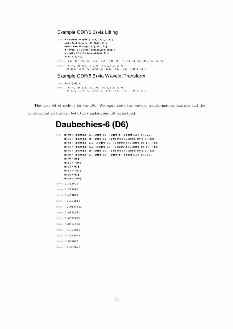
In[72]:= MatrixForm@[email protected]@LG2@12DDDMatrixForm@[email protected]@LG1@12DDD
Out[72]//MatrixForm=1 0 0 0 0 0 0 0 0 0 0 00 1 0 0 0 0 0 0 0 0 0 00 0 1 0 0 0 0 0 0 0 0 00 0 0 1 0 0 0 0 0 0 0 00 0 0 0 1 0 0 0 0 0 0 00 0 0 0 0 1 0 0 0 0 0 00 0 0 0 0 0 1 0 0 0 0 00 0 0 0 0 0 0 1 0 0 0 00 0 0 0 0 0 0 0 1 0 0 00 0 0 0 0 0 0 0 0 1 0 00 0 0 0 0 0 0 0 0 0 1 00 0 0 0 0 0 0 0 0 0 0 1
Out[73]//MatrixForm=1 0 0 0 0 0 0 0 0 0 0 00 1 0 0 0 0 0 0 0 0 0 00 0 1 0 0 0 0 0 0 0 0 00 0 0 1 0 0 0 0 0 0 0 00 0 0 0 1 0 0 0 0 0 0 00 0 0 0 0 1 0 0 0 0 0 00 0 0 0 0 0 1 0 0 0 0 00 0 0 0 0 0 0 1 0 0 0 00 0 0 0 0 0 0 0 1 0 0 00 0 0 0 0 0 0 0 0 1 0 00 0 0 0 0 0 0 0 0 0 1 00 0 0 0 0 0 0 0 0 0 0 1
Example CDF(5,3) via LiftingIn[74]:= v = RandomInteger@8-128, 127<, 816<D
odd = Partition@v, 2D@@All, 1DD;even = Partition@v, 2D@@All, 2DD;d = even - 1 ê 2 Hodd + RotateLeft@oddDL;s = odd + 1 ê 4 Hd + RotateRight@dDL;N@Join@s, dDD
Out[74]= 8-24, -46, -82, 30, -115, -114, -125, 66, -7, -55, 61, 56, 113, -69, 30, 53<Out[79]= 8-9.75, -48.125, -81.375, -90.5, 5.5, 32.75,
70.125, 7.375, 7., 128.5, 6., 132., -82., -31., -140.5, 50.<Example CDF(5,3) via Wavelet TransformIn[80]:= N@[email protected][80]= 8-9.75, -48.125, -81.375, -90.5, 5.5, 32.75,
70.125, 7.375, 7., 128.5, 6., 132., -82., -31., -140.5, 50.<
CDF(5,3).nb 3
The next set of code is for the D6. We again state the wavelet transformation matrices and the
implementation through both the standard and lifting method.
Daubechies-6 (D6)In[15]:= N@h0 = HSqrt@2D H1 + Sqrt@10D + Sqrt@5 + 2 Sqrt@10DDLL ê 32D
N@h1 = HSqrt@2D H5 + Sqrt@10D + 3 Sqrt@5 + 2 Sqrt@10DDLL ê 32DN@h2 = HSqrt@2D H10 - 2 Sqrt@10D + 2 Sqrt@5 + 2 Sqrt@10DDLL ê 32DN@h3 = HSqrt@2D H10 - 2 Sqrt@10D - 2 Sqrt@5 + 2 Sqrt@10DDLL ê 32DN@h4 = HSqrt@2D H5 + Sqrt@10D - 3 Sqrt@5 + 2 Sqrt@10DDLL ê 32DN@h5 = HSqrt@2D H1 + Sqrt@10D - Sqrt@5 + 2 Sqrt@10DDLL ê 32DN@g0 = h5DN@g1 = -h4DN@g2 = h3DN@g3 = -h2DN@g4 = h1DN@g5 = -h0D
Out[15]= 0.332671
Out[16]= 0.806892
Out[17]= 0.459878
Out[18]= -0.135011
Out[19]= -0.0854413
Out[20]= 0.0352263
Out[21]= 0.0352263
Out[22]= 0.0854413
Out[23]= -0.135011
Out[24]= -0.459878
Out[25]= 0.806892
Out[26]= -0.332671
56
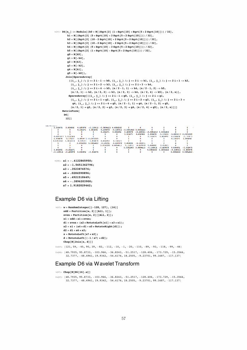
In[37]:= D6@n_D := Module@8h0 = N@HSqrt@2D H1 + Sqrt@10D + Sqrt@5 + 2 Sqrt@10DDLL ê 32D,h1 = N@HSqrt@2D H5 + Sqrt@10D + 3 Sqrt@5 + 2 Sqrt@10DDLL ê 32D,h2 = N@HSqrt@2D H10 - 2 Sqrt@10D + 2 Sqrt@5 + 2 Sqrt@10DDLL ê 32D,h3 = N@HSqrt@2D H10 - 2 Sqrt@10D - 2 Sqrt@5 + 2 Sqrt@10DDLL ê 32D,h4 = N@HSqrt@2D H5 + Sqrt@10D - 3 Sqrt@5 + 2 Sqrt@10DDLL ê 32D,h5 = N@HSqrt@2D H1 + Sqrt@10D - Sqrt@5 + 2 Sqrt@10DDLL ê 32D,g0 = N@h5D,g1 = N@-h4D,g2 = N@h3D,g3 = N@-h2D,g4 = N@h1D,g5 = N@-h0D<,
Join@SparseArray@88i_, j_< ê; j == 2 i - 1 -> h0, 8i_, j_< ê; j == 2 i -> h1, 8i_, j_< ê; j == 2 i + 1 -> h2,
8i_, j_< ê; j == 2 i + 2 -> h3, 8i_, j_< ê; j == 2 i + 3 -> h4,
8i_, j_< ê; j == 2 i + 4 -> h5, 8n ê 2 - 1, 1< -> h4, 8n ê 2 - 1, 2< -> h5,8n ê 2, 1< -> h2, 8n ê 2, 2< -> h3, 8n ê 2, 3< -> h4, 8n ê 2, 4< -> h5<, 8n ê 2, n<D,
SparseArray@88i_, j_< ê; j == 2 i - 1 Æ g0, 8i_, j_< ê; j == 2 i Æ g1,
8i_, j_< ê; j == 2 i + 1 Æ g2, 8i_, j_< ê; j == 2 i + 2 Æ g3, 8i_, j_< ê; j == 2 i + 3 Æ
g4, 8i_, j_< ê; j == 2 i + 4 Æ g5, 8n ê 2 - 1, 1< Æ g4, 8n ê 2 - 1, 2< Æ g5,
8n ê 2, 1< Æ g2, 8n ê 2, 2< Æ g3, 8n ê 2, 3< Æ g4, 8n ê 2, 4< Æ g5<, 8n ê 2, n<DDDMatrixForm@D6@12DD
Out[38]//MatrixForm=0.332671 0.806892 0.459878 -0.135011 -0.0854413 0.0352263 0
0 0 0.332671 0.806892 0.459878 -0.135011 -0.0854413 0.03522630 0 0 0 0.332671 0.806892 0.459878 -0.1350110 0 0 0 0 0 0.332671 0.806892
-0.0854413 0.0352263 0 0 0 0 00.459878 -0.135011 -0.0854413 0.0352263 0 0 00.0352263 0.0854413 -0.135011 -0.459878 0.806892 -0.332671 0
0 0 0.0352263 0.0854413 -0.135011 -0.459878 0.806892 -0.3326710 0 0 0 0.0352263 0.0854413 -0.135011 -0.4598780 0 0 0 0 0 0.0352263 0.0854413
0.806892 -0.332671 0 0 0 0 0-0.135011 -0.459878 0.806892 -0.332671 0 0 0
In[39]:= a1 = -.4122865950;
a2 = -1.5651362796;
a3 = .3523876576;
a4 = .0284590896;
a5 = .4921518449;
a6 = -.3896203900;
a7 = 1.9182029462;
2 D6.nb
Example D6 via LiftingIn[57]:= w = RandomInteger@8-128, 127<, 816<D
odd = Partition@w, 2D@@All, 1DD;even = Partition@w, 2D@@All, 2DD;s1 = odd + a1 * even;
d1 = even + Ha2 * RotateLeft@s1D + a3 * s1L;s2 = s1 + Ha4 * d1 + a5 * RotateRight@d1DL;d2 = d1 + a6 * s2;
s = RotateLeft@a7 * s2D;d = RotateLeft@H-1 ê a7L * d2D;Chop@N@Join@s, dDDD
Out[57]= 8121, 59, -45, 90, 39, -82, -112, -10, -1, -20, -110, -89, -93, -118, -99, -46<Out[66]= 848.7935, 95.8733, -103.966, -36.8243, -51.2517, -128.406, -173.729, -15.3566,
32.7377, -48.4961, 19.9342, -54.6176, 18.2505, -9.23701, 99.1687, -117.137<Example D6 via Wavelet TransformIn[67]:= Chop@N@[email protected][67]= 848.7935, 95.8733, -103.966, -36.8243, -51.2517, -128.406, -173.729, -15.3566,
32.7377, -48.4961, 19.9342, -54.6176, 18.2505, -9.23701, 99.1687, -117.137<
D6.nb 3
57
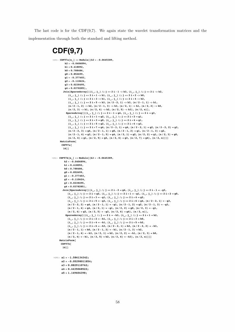
The last code is for the CDF(9,7). We again state the wavelet transformation matrices and the
implementation through both the standard and lifting method.
CDF(9,7)In[83]:= CDF97a@n_D := Module@8h3 = -0.0645389,
h2 = -0.0406894,
h1 = 0.418092,
h0 = 0.788486,
g0 = 0.852699,
g1 = -0.377403,
g2 = -0.110624,
g3 = 0.0238495,
g4 = 0.0378285<,Join@SparseArray@88i_, j_< ê; j == 2 i - 1 -> h3, 8i_, j_< ê; j == 2 i -> h2,
8i_, j_< ê; j == 2 i + 1 -> h1, 8i_, j_< ê; j == 2 i + 2 -> h0,
8i_, j_< ê; j == 2 i + 3 -> h1, 8i_, j_< ê; j == 2 i + 4 -> h2,
8i_, j_< ê; j == 2 i + 5 -> h3, 8n ê 2 - 2, 1< -> h3, 8n ê 2 - 1, 1< -> h1,8n ê 2 - 1, 2< -> h2, 8n ê 2 - 1, 3< -> h3, 8n ê 2, 1< -> h1, 8n ê 2, 2< -> h0,8n ê 2, 3< -> h1, 8n ê 2, 4< -> h2, 8n ê 2, 5< -> h3<, 8n ê 2, n<D,
SparseArray@88i_, j_< ê; j == 2 i - 1 Æ g4, 8i_, j_< ê; j == 2 i Æ g3,
8i_, j_< ê; j == 2 i + 1 Æ g2, 8i_, j_< ê; j == 2 i + 2 Æ g1,
8i_, j_< ê; j == 2 i + 3 Æ g0, 8i_, j_< ê; j == 2 i + 4 Æ g1,
8i_, j_< ê; j == 2 i + 5 Æ g2, 8i_, j_< ê; j == 2 i + 6 Æ g3,
8i_, j_< ê; j == 2 i + 7 Æ g4, 8n ê 2 - 3, 1< Æ g4, 8n ê 2 - 2, 1< Æ g2, 8n ê 2 - 2, 2< Æ g3,
8n ê 2 - 2, 3< Æ g4, 8n ê 2 - 1, 1< Æ g0, 8n ê 2 - 1, 2< Æ g1, 8n ê 2 - 1, 3< Æ g2,8n ê 2 - 1, 4< Æ g3, 8n ê 2 - 1, 5< Æ g4, 8n ê 2, 1< Æ g2, 8n ê 2, 2< Æ g1, 8n ê 2, 3< Æ g0,8n ê 2, 4< Æ g1, 8n ê 2, 5< Æ g2, 8n ê 2, 6< Æ g3, 8n ê 2, 7< Æ g4<, 8n ê 2, n<DDDMatrixForm@CDF97a@16DD
Out[84]//MatrixForm=-0.0645389 -0.0406894 0.418092 0.788486 0.418092 -0.0406894 -0.0645389
0 0 -0.0645389 -0.0406894 0.418092 0.788486 0.418092 -0 0 0 0 -0.0645389 -0.0406894 0.4180920 0 0 0 0 0 -0.0645389 -0 0 0 0 0 0 0
-0.0645389 0 0 0 0 0 00.418092 -0.0406894 -0.0645389 0 0 0 00.418092 0.788486 0.418092 -0.0406894 -0.0645389 0 00.0378285 0.0238495 -0.110624 -0.377403 0.852699 -0.377403 -0.110624 0.0238495
0 0 0.0378285 0.0238495 -0.110624 -0.377403 0.852699 -0 0 0 0 0.0378285 0.0238495 -0.110624 -0 0 0 0 0 0 0.0378285 0.0238495
0.0378285 0 0 0 0 0 0-0.110624 0.0238495 0.0378285 0 0 0 00.852699 -0.377403 -0.110624 0.0238495 0.0378285 0 0
-0.110624 -0.377403 0.852699 -0.377403 -0.110624 0.0238495 0.0378285
In[85]:= CDF97b@n_D := Module@8h3 = -0.0645389,h2 = -0.0406894,
h1 = 0.418092,
h0 = 0.788486,
g0 = 0.852699,
g1 = -0.377403,
g2 = -0.110624,
g3 = 0.0238495,
g4 = 0.0378285<,Join@SparseArray@88i_, j_< ê; j == 2 i - 2 Æ g4, 8i_, j_< ê; j == 2 i - 1 Æ -g3,
8i_, j_< ê; j == 2 i Æ g2, 8i_, j_< ê; j == 2 i + 1 Æ -g1, 8i_, j_< ê; j == 2 i + 2 Æ g0,
8i_, j_< ê; j == 2 i + 3 Æ -g1, 8i_, j_< ê; j == 2 i + 4 Æ g2,
8i_, j_< ê; j == 2 i + 5 Æ -g3, 8i_, j_< ê; j == 2 i + 6 Æ g4, 8n ê 2 - 2, 1< Æ -g3,8n ê 2 - 2, 2< Æ g4, 8n ê 2 - 1, 1< Æ -g1, 8n ê 2 - 1, 2< Æ g2, 8n ê 2 - 1, 3< Æ -g3,8n ê 2 - 1, 4< Æ g4, 8n ê 2, 1< Æ -g1, 8n ê 2, 2< Æ g0, 8n ê 2, 3< Æ -g1,8n ê 2, 4< Æ g2, 8n ê 2, 5< Æ -g3, 8n ê 2, 6< Æ g4<, 8n ê 2, n<D,
SparseArray@88i_, j_< ê; j == 2 i Æ -h3, 8i_, j_< ê; j == 2 i + 1 Æ h2,
8i_, j_< ê; j == 2 i + 2 Æ -h1, 8i_, j_< ê; j == 2 i + 3 Æ h0,
8i_, j_< ê; j == 2 i + 4 Æ -h1, 8i_, j_< ê; j == 2 i + 5 Æ h2,
8i_, j_< ê; j == 2 i + 6 Æ -h3, 8n ê 2 - 2, 1< Æ h2, 8n ê 2 - 2, 2< Æ -h3,8n ê 2 - 1, 1< Æ h0, 8n ê 2 - 1, 2< Æ -h1, 8n ê 2 - 1, 3< Æ h2,8n ê 2 - 1, 4< Æ -h3, 8n ê 2, 1< Æ h2, 8n ê 2, 2< Æ -h1, 8n ê 2, 3< Æ h0,8n ê 2, 4< Æ -h1, 8n ê 2, 5< Æ h2, 8n ê 2, 6< Æ -h3<, 8n ê 2, n<DDD
MatrixForm@CDF97b@16DD
Out[86]//MatrixForm=-0.0238495 -0.110624 0.377403 0.852699 0.377403 -0.110624 -0.0238495 0.0378285
0 0.0378285 -0.0238495 -0.110624 0.377403 0.852699 0.377403 -0.1106240 0 0 0.0378285 -0.0238495 -0.110624 0.377403 0.8526990 0 0 0 0 0.0378285 -0.0238495 -0.1106240 0 0 0 0 0 0 0.0378285
-0.0238495 0.0378285 0 0 0 0 00.377403 -0.110624 -0.0238495 0.0378285 0 0 00.377403 0.852699 0.377403 -0.110624 -0.0238495 0.0378285 0
0 0.0645389 -0.0406894 -0.418092 0.788486 -0.418092 -0.0406894 0.06453890 0 0 0.0645389 -0.0406894 -0.418092 0.788486 -0.4180920 0 0 0 0 0.0645389 -0.0406894 -0.4180920 0 0 0 0 0 0 0.06453890 0 0 0 0 0 0
-0.0406894 0.0645389 0 0 0 0 00.788486 -0.418092 -0.0406894 0.0645389 0 0 0
-0.0406894 -0.418092 0.788486 -0.418092 -0.0406894 0.0645389 0
2 CDF(9,7).nb
In[87]:= Chop@MatrixForm@[email protected]@CDF97b@16DDDDChop@MatrixForm@[email protected]@CDF97a@16DDDD
Out[87]//MatrixForm=1. 2.10523 ¥ 10-7 7.2059 ¥ 10-9 1.52765 ¥ 10-9 0 1.52765 ¥ 10-9
2.10523 ¥ 10-7 1. 2.10523 ¥ 10-7 7.2059 ¥ 10-9 1.52765 ¥ 10-9 07.2059 ¥ 10-9 2.10523 ¥ 10-7 1. 2.10523 ¥ 10-7 7.2059 ¥ 10-9 1.52765 ¥ 10-9
1.52765 ¥ 10-9 7.2059 ¥ 10-9 2.10523 ¥ 10-7 1. 2.10523 ¥ 10-7 7.2059 ¥ 10-9
0 1.52765 ¥ 10-9 7.2059 ¥ 10-9 2.10523 ¥ 10-7 1. 2.10523 ¥ 10-7
0.00153922 0 1.52765 ¥ 10-9 7.2059 ¥ 10-9 2.10523 ¥ 10-7 1.-0.0298272 1.52765 ¥ 10-9 0 1.52765 ¥ 10-9 7.2059 ¥ 10-9 2.10523 ¥ 10-7
0.00153943 7.2059 ¥ 10-9 1.52765 ¥ 10-9 0 1.52765 ¥ 10-9 7.2059 ¥ 10-9
0 0 0 0 0 00 0 0 0 0 00 0 0 0 0 00 0 0 0 0 0
-0.000902191 0 0 0 0 00.0142766 0 0 0 0 00.0142766 0 0 0 0 0
-0.000902191 0 0 0 0 0
Out[88]//MatrixForm=
1. 2.10523 ¥ 10-7 7.2059 ¥ 10-9 1.52765 ¥ 10-9 0 0.001539222.10523 ¥ 10-7 1. 2.10523 ¥ 10-7 7.2059 ¥ 10-9 1.52765 ¥ 10-9 07.2059 ¥ 10-9 2.10523 ¥ 10-7 1. 2.10523 ¥ 10-7 7.2059 ¥ 10-9 1.52765 ¥ 10-9
1.52765 ¥ 10-9 7.2059 ¥ 10-9 2.10523 ¥ 10-7 1. 2.10523 ¥ 10-7 7.2059 ¥ 10-9
0 1.52765 ¥ 10-9 7.2059 ¥ 10-9 2.10523 ¥ 10-7 1. 2.10523 ¥ 10-7
1.52765 ¥ 10-9 0 1.52765 ¥ 10-9 7.2059 ¥ 10-9 2.10523 ¥ 10-7 1.7.2059 ¥ 10-9 1.52765 ¥ 10-9 0 1.52765 ¥ 10-9 7.2059 ¥ 10-9 2.10523 ¥ 10-7
2.10523 ¥ 10-7 7.2059 ¥ 10-9 1.52765 ¥ 10-9 0 1.52765 ¥ 10-9 7.2059 ¥ 10-9
0 0 0 0 0 00 0 0 0 0 00 0 0 0 0 00 0 0 0 0 00 0 0 0 0 00 0 0 0 0 00 0 0 0 0 00 0 0 0 0 0
In[89]:= a1 = -1.586134342;
a2 = -0.05298011854;
a3 = 0.8829110762;
a4 = 0.4435068522;
a5 = 1.149604398;
CDF(9,7).nb 3
58

In[209]:= v = RandomInteger@8-128, 127<, 816<Dodd = Partition@v, 2D@@All, 1DD;even = Partition@v, 2D@@All, 2DD;d1 = odd + a1 * Heven + RotateRight@evenDL;s1 = even + a2 * Hd1 + RotateLeft@d1DL;d2 = d1 + a3 * Hs1 + RotateRight@s1DL;s2 = s1 + a4 * Hd2 + RotateLeft@d2DL;s = RotateLeft@a5 * s2D;d = RotateLeft@d2 ê a5, 2D;N@Join@s, dDD
Out[209]= 826, -49, -125, -110, 41, 58, -106, -107, -97, 67, 28, -66, -55, 24, 23, 14<Out[218]= 8-128.104, 54.9063, -189.983, 57.1697, -78.288, 13.5334, 30.8312, -66.9496,
53.3999, -63.5895, -57.102, 22.4876, -22.6543, -3.99432, 33.7338, -30.1634<In[219]:= [email protected][219]= 8-128.634, 54.9063, -189.983, 57.1697, -78.288, 13.5334, 30.8312, -66.9497,
53.3999, -63.5896, -57.102, 22.4876, -22.6544, -3.9943, 33.7338, -30.1635<
4 CDF(9,7).nb
59

List of Figures
1 Periodic function f . . . . . . . . . . . . . . . . . . . . . . . . . . . . . . . . . . . . . . . . 7
2 Partial sum (S5) . . . . . . . . . . . . . . . . . . . . . . . . . . . . . . . . . . . . . . . . . 7
3 Partial sum (S10) . . . . . . . . . . . . . . . . . . . . . . . . . . . . . . . . . . . . . . . . . 7
4 Plot of φ0 . . . . . . . . . . . . . . . . . . . . . . . . . . . . . . . . . . . . . . . . . . . . . 25
5 Plot of φ1 . . . . . . . . . . . . . . . . . . . . . . . . . . . . . . . . . . . . . . . . . . . . . 26
6 Plot of φ2 . . . . . . . . . . . . . . . . . . . . . . . . . . . . . . . . . . . . . . . . . . . . . 26
7 Plot of φ4 . . . . . . . . . . . . . . . . . . . . . . . . . . . . . . . . . . . . . . . . . . . . . 26
8 Plot of φ6 . . . . . . . . . . . . . . . . . . . . . . . . . . . . . . . . . . . . . . . . . . . . . 26
9 Mean and difference (bold) computations for x. . . . . . . . . . . . . . . . . . . . . . . . 27
10 One step of lifting . . . . . . . . . . . . . . . . . . . . . . . . . . . . . . . . . . . . . . . . 28
11 Two lifting steps . . . . . . . . . . . . . . . . . . . . . . . . . . . . . . . . . . . . . . . . . 29
12 Cost of Lifting vs. Standard algorithms . . . . . . . . . . . . . . . . . . . . . . . . . . . . 49
60

Curriculum Vita
Adrian Delgado was born in El Paso, Texas. The second son of Mario and Miriam Delgado, he graduated
J.M. Hanks High School, El Paso, Texas in the spring of 2006. He enrolled at University of Texas at
El Paso in the fall of 2007. While pursuing a bachelor’s degree in mathematics, he worked as a tutor
and peer leader for freshmen mathematics courses. After completing a student internship at Montwood
HIgh School, El Paso, Texas, he received his bachelor’s of science degree from University of Texas at El
Paso in the spring of 2010. Eager to further his studies in mathematics, in the fall of 2010 he enrolled in
Graduate School at the University of Texas at El Paso in the Department of Mathematics.
61