Life-Cycle Cost Analysisin Pavement Design

- In Search of Better Investment Decisions -

Pavement Division Interim Technical BulletinSeptember 1998

Publication No. FHWA-SA-98-079

This Interim Technical Bulletin presents technical guidance and recommendations on good/bestpractices in conducting Life-Cycle Cost Analysis (LCCA) in pavement design. The Bulletin will be ofinterest to State highway agency personnel responsible for conducting and/or reviewing pavementdesign LCCAs.

To reinforce this publication, the FHWA Office of Engineering, Pavement Division, in cooperation withthe Office of Technology Applications, offers LCCA technical support through FHWA DemonstrationProject No.115, Probabilistic LCCA in Pavement Design (DP-115). DP-115 is a free 2-dayworkshop that demonstrates good/best practices in performing life-cycle cost analyses for pavementdesign. This workshop is available, upon request, to State highway agencies.

This publication and DP-115 support the FHWA’s response to the Transportation Equity Act for the21st Century legislative mandate to develop recommended procedures for conducting LCCA onNational Highway System projects.

Henry H. Rentz, DirectorOffice of EngineeringFederal Highway Administration

The United States Government does not endorse products or manufacturers. Trade or manufacturers’names appear herein only because they are considered essential to the objective of this document.

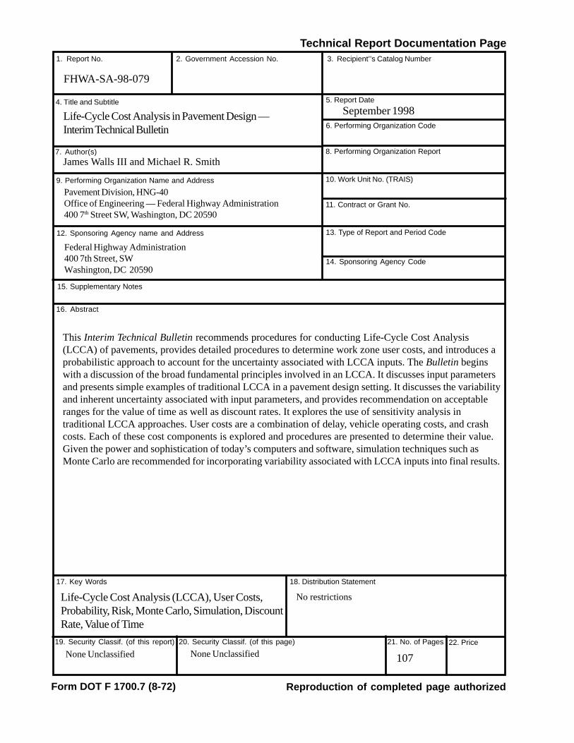
1. Report No. 2. Government Accession No. 3. Recipient’’s Catalog Number

4. Title and Subtitle 5. Report Date

6. Performing Organization Code

7. Author(s) 8. Performing Organization Report

10. Work Unit No. (TRAIS)9. Performing Organization Name and Address

12. Sponsoring Agency name and Address

11. Contract or Grant No.

13. Type of Report and Period Code

14. Sponsoring Agency Code

15. Supplementary Notes

16. Abstract

17. Key Words 18. Distribution Statement

19. Security Classif. (of this report) 20. Security Classif. (of this page) 21. No. of Pages 22. Price

Form DOT F 1700.7 (8-72) Reproduction of completed page authorized

Technical Report Documentation Page

Life-Cycle Cost Analysis in Pavement Design —Interim Technical Bulletin

September 1998

James Walls III and Michael R. Smith

Pavement Division, HNG-40Office of Engineering — Federal Highway Administration400 7th Street SW, Washington, DC 20590

Federal Highway Administration400 7th Street, SWWashington, DC 20590

This Interim Technical Bulletin recommends procedures for conducting Life-Cycle Cost Analysis(LCCA) of pavements, provides detailed procedures to determine work zone user costs, and introduces aprobabilistic approach to account for the uncertainty associated with LCCA inputs. The Bulletin beginswith a discussion of the broad fundamental principles involved in an LCCA. It discusses input parametersand presents simple examples of traditional LCCA in a pavement design setting. It discusses the variabilityand inherent uncertainty associated with input parameters, and provides recommendation on acceptableranges for the value of time as well as discount rates. It explores the use of sensitivity analysis intraditional LCCA approaches. User costs are a combination of delay, vehicle operating costs, and crashcosts. Each of these cost components is explored and procedures are presented to determine their value.Given the power and sophistication of today’s computers and software, simulation techniques such asMonte Carlo are recommended for incorporating variability associated with LCCA inputs into final results.

Life-Cycle Cost Analysis (LCCA), User Costs,Probability, Risk, Monte Carlo, Simulation, DiscountRate, Value of Time

No restrictions

None Unclassified None Unclassified 107

FHWA-SA-98-079

ii

iii

Life-Cycle Cost Analysisin Pavement Design

- In Search of Better Investment Decisions -

Pavement Division Interim Technical BulletinSeptember 1998

iv

The authors appreciate the following individuals who reviewed this Bulletin:

Richard Clark – Montana Department of TransportationGaylord Cumberledge – Pennsylvania Department of Transportation (retired)Dale Decker – National Asphalt Pavement AssociationRoger Green – Ohio Department of TransportationJames W. Mack – American Concrete Pavement AssociationJoseph Mahoney – University of WashingtonLarry Scofield – Arizona Transportation Research Council

The authors are grateful for the special support received from the Pennsylvania Department ofTransportation for use of its user cost procedures as a framework for developing the User Costchapter of this Bulletin.

ACKNOWLEDGMENTS

v

EXECUTIVE SUMMARY...................................................................................... xi-xiv

Chapter 1. INTRODUCTION ...................................................................................... 1SCOPE ....................................................................................................................................................... 1APPLICATION .............................................................................................................................................. 1LEVEL OF DETAIL ........................................................................................................................................ 2LCCA DRIVING FORCES .............................................................................................................................. 2GENERAL DEFINITIONS ................................................................................................................................ 3ELIMINATE INDICATORS ................................................................................................................................ 4DISCOUNT RATES ........................................................................................................................................ 5COST ESTIMATES .......................................................................................................................................... 5DISCOUNT RATES ........................................................................................................................................ 5

Nominal Versus Real ...................................................................................................................... 5Values to Use ................................................................................................................................. 6

STRUCTURED APPROACH ............................................................................................................................. 7

Chapter 2. LCCA PROCEDURES ............................................................................... 9ESTABLISH ALTERNATIVE PAVEMENT DESIGN STRATEGIES FOR THE ANALYSIS PERIOD ........................................ 9DETERMINE PERFORMANCE PERIODS AND ACTIVITY TIMING ...........................................................................10ESTIMATE AGENCY COSTS ...........................................................................................................................12ESTIMATE USER COSTS ................................................................................................................................13

Normal Operations Versus Work Zones .......................................................................................13User Cost Rates ............................................................................................................................16Delay Cost Rates (Value of Time) ................................................................................................19Crash Cost Rates ..........................................................................................................................23

DEVELOP EXPENDITURE STREAM DIAGRAMS ................................................................................................24COMPUTE NET PRESENT VALUE (NPV) ........................................................................................................25ANALYZE RESULTS .....................................................................................................................................27REEVALUATE DESIGN STRATEGY ..................................................................................................................31

Chapter 3. WORK ZONE USER COSTS .................................................................. 33WORK ZONE USER COSTS ..........................................................................................................................33WORK ZONE DEFINED ...............................................................................................................................33WORK ZONE CHARACTERISTICS ..................................................................................................................34TRAFFIC CHARACTERISTICS ..........................................................................................................................34

AADT ...........................................................................................................................................35Traffic Diversion ...........................................................................................................................35Vehicle Classification ....................................................................................................................37Directional Hourly Traffic Distribution .........................................................................................37

CONCEPTUAL ANALYSIS .............................................................................................................................39Free Flow ......................................................................................................................................39Forced Flow (Level of Service F) ..................................................................................................41

COMPUTATIONAL ANALYSIS ........................................................................................................................42Example Work Zone Problem Defined ...........................................................................................42Step 1. Project Future Year Traffic Demand ..................................................................................43Step 2. Calculate Work Zone Directional Hourly Demand ............................................................43Step 3. Determine Roadway Capacity ...........................................................................................44Step 4. Identify the User Cost Components .................................................................................51

CONTENTS

vi

Step 5. Quantify Traffic Affected by Each Cost Component ........................................................54Step 6. Compute Reduced Speed Delay ........................................................................................57Step 7. Select and Assign VOC Rates ...........................................................................................64Step 8. Select and Assign Delay Cost Rates ................................................................................65Step 9. Assign Traffic to Vehicle Classes .....................................................................................65Step 10. Compute User Cost Components by Vehicle Class .........................................................66Step 11. Sum Total Work Zone User Costs ...................................................................................69Step 12. Address Circuity and Delay Costs ..................................................................................70

CIRCUITY ...................................................................................................................................................71CRASH COSTS ............................................................................................................................................72

General ..........................................................................................................................................72Overall Crash Rates ......................................................................................................................73Work Zone Crash Rates ................................................................................................................74Example Crash Cost Calculations .................................................................................................78

Chapter 4. RISK ANALYSIS APPROACH............................................................... 81DEFINING RISK ..........................................................................................................................................81DEFINING RISK ANALYSIS ...........................................................................................................................81THE NEED FOR RISK ANALYSIS ...................................................................................................................81GENERAL APPROACH .................................................................................................................................82

Step 1. Identify the Structure and Layout of the Problem ............................................................85Step 2. Quantify Uncertainty Using Probability ..........................................................................87Step 3. Perform Simulation ...........................................................................................................92Step 4. Analyze and Interpret Results .........................................................................................96Step 5. Make Consensus Decision ............................................................................................ 101

PRESENTING RISK ANALYSIS RESULTS ........................................................................................................ 101

REFERENCES ........................................................................................................... 103

APPENDIX: RESOURCES ....................................................................................... 105PUBLICATIONS .......................................................................................................................................... 105COMPUTER SOFTWARE .............................................................................................................................. 107

vii

Figure 1. 1 Historical trends on 10-year Treasury notes. ............................................................................. 6

Figure 2. 1 Analysis period for a pavement design alternative. ..................................................................10Figure 2. 2 Performance curve versus rehabilitation strategy. .....................................................................14Figure 2. 3 Effect of roughness on road user costs in New Zealand. ..........................................................15Figure 2. 4 Typical expenditure stream diagram for a pavement design alternative. ....................................24Figure 2. 5 Expenditure stream diagram for agency and user costs. ............................................................26Figure 2. 6 Sensitivity of NPV to discount rate. ..........................................................................................29

Figure 3. 1 Free-flow cost components. ......................................................................................................40Figure 3. 2 Forced-flow cost components level of service F. ......................................................................41Figure 3. 3 Range of observed work zone capacities. ..................................................................................49Figure 3. 4 Cumulative distribution of observed work zone capacities. ......................................................50Figure 3. 5 Average speed versus V/C ratio (level of service F). .................................................................59Figure 3. 6 Queued vehicle growth and dissipation over time. ................................................................... 60Figure 3. 7 Average number of queued vehicles in each hour. ....................................................................61

Figure 4. 1 Computation of NPV using probability and simulation. ............................................................83Figure 4. 2 Pavement life curves for Alternatives A and B. .........................................................................85Figure 4. 3 Cash flow diagram for Alternatives A and B. ............................................................................86Figure 4. 4 Example probability distributions. ................................................................................. ............87Figure 4. 5 Ascending cumulative probability distribution. ........................................................................87Figure 4. 6 Using expert opinion to develop probability distributions. .......................................................88Figure 4. 7 Excel spreadsheet showing @RISK add-in buttons. .................................................................91Figure 4. 8 Monte Carlo sampling showing four iterations. ........................................................................92Figure 4. 9 Latin Hypercube sampling showing four iterations. .................................................................. 93Figure 4.10 Monte Carlo sampling – 100 iterations. ....................................................................................94Figure 4.11 Latin Hypercube sampling – 100 iterations. ..............................................................................94Figure 4.12 Histogram NPV for Alternatives A and B. ................................................................................96Figure 4.13 Cumulative risk profile of net present value for Alternatives A and B. ....................................97Figure 4.14 Correlation sensitivity plot for NPV Alternative A. ..................................................................99Figure 4.15 Correlation sensitivity plot for NPV Alternative B. ...................................................................99Figure 4.16 Analysis of distribution tails. ................................................................................................. 100

FIGURES

viii

Table 1.1 Recent trends in OMB real discount rates. ................................................................................... 7

Table 2.1 PennDOT’s design strategy for new, reconstructed, and unbonded overlay. .............................11Table 2.2 Added time and vehicle running cost /1,000 stops and idling costs (1970 $). .............................17Table 2.3 Added time and vehicle running cost /1,000 stops and idling costs (Aug 96 $). .........................18Table 2.4 Speed change computations. .......................................................................................................18Table 2.5 Updated NCHRP 133 values of time ($/Veh-Hr) (Aug 96 $). .........................................................19Table 2.6 Updated MicroBENCOST default values of time ($/Veh-Hr) (Aug 96 $). .....................................20Table 2.7 Composite earlier research value of time ($/Veh-Hr) (Aug 96 $). ..................................................20Table 2.8 Travel time ranges as a percent of national wage rate (1995 $/Person-Hr). ..................................21Table 2.9 OST-recommended hourly wage rates (1995 $/Person-Hr). ..........................................................21Table 2.10 Ranges for hourly values of travel time (1995 $/Person-Hr). ......................................................21Table 2.11 Value of one vehicle hour of travel time (1995 $). .......................................................................22Table 2.12 Composite listing of travel time values. .....................................................................................23Table 2.13 Recommended values of time ($/Veh-Hr) (Aug 96 $). .................................................................23Table 2.14 MicroBENCOST default crash cost rates ($1,000, 1990 $). .........................................................23Table 2.15 MicroBENCOST default crash cost rates ($1,000, Aug 96 $). ....................................................24Table 2.16 Present value discount factors: single future payment. .............................................................26Table 2.17 NPV calculation using 4 percent discount rate factors. .............................................................27Table 2.18 Sensitivity analysis – Alternative # 1. ........................................................................................28Table 2.19 Sensitivity analysis – Alternative # 2. ........................................................................................28Table 2.20 Comparison of alternative NPVs ($1,000) to discount rate. ........................................................29Table 2.21 Sensitivity to user cost and discount rate. .................................................................................30

Table 3.1 Default hourly distributions from MicroBENCOST (all functional classes). ................................38Table 3.2 PennDOT AADT distribution (hourly percentages). ...................................................................39Table 3.3 Work zone directional hourly demand (all vehicle classes). .........................................................44Table 3.4 Truck equivalency factors. ..........................................................................................................46Table 3.5 Maximum mixed vehicle traffic capacities for trucks in the traffic stream

(4-lane facilities). .........................................................................................................................47Table 3.6 Maximum mixed vehicle traffic capacities for trucks in the traffic stream

(6 or more lanes). .........................................................................................................................47Table 3.7 Observed saturation flow rates per hour of green time. ............................................................... 48Table 3.8 Measured average work zone capacities. .....................................................................................49Table 3.9 Work zone analysis matrix. ...........................................................................................................51Table 3.10 Expanded work zone matrix. .......................................................................................................54Table 3.11 Summary traffic affected by each cost component. ...................................................................57Table 3.12 Work zone reduced speed delay. ................................................................................................58Table 3.13 Queue speed. .............................................................................................................................58Table 3.14 Average queue length calculations. ...........................................................................................62Table 3.15 Average queue length – alternative approach. ..........................................................................63

TABLES

ix

Table 3.16 Average queue delay time. .........................................................................................................64Table 3.17 Added time and vehicle running cost/1,000 stops and idling costs (Aug 96 $). ........................64Table 3.18 Speed change computations. .....................................................................................................65Table 3.19 Recommended values of travel time ($/Veh-Hr) (Aug 96). ..........................................................65Table 3.20 Affected traffic by vehicle class and user cost component. ......................................................66Table 3.21 User cost component # 1 - speed change VOC (55-40-55 mi/h). .................................................66Table 3.22 User cost component # 2 - speed change delay cost (55-40-55 mi/h). ........................................67Table 3.23 User cost component # 3 - work zone reduced speed delay cost. ..............................................67Table 3.24 User cost component # 4 - stopping VOC (55-0-55 mi/h). ..........................................................67Table 3.25 User cost component # 5 - stopping delay cost (55-0-55 mi/h). .................................................67Table 3.26 User cost component # 6 - idling VOC. ......................................................................................68Table 3.27 User cost component # 7 - queue reduced speed delay cost. ....................................................68Table 3.28 Master summary - total (60 day) work zone user cost (Aug 96 $). .............................................69Table 3.29 Master summary - work zone user cost distribution (%). ...........................................................69Table 3.30 Average weekday delay – North Ridge earthquake. ..................................................................70Table 3.31 1995 people injured in motor vehicle crashes by functional class. .............................................73Table 3.32 1995 vehicles miles of travel (millions). ......................................................................................73Table 3.33 Crash injury rates (people injured per 100 M VMT). .................................................................. 74Table 3.34 1996 work zone motor vehicles crash fatalities as a percent of all fatalities. ...............................75Table 3.35 Crash rates on SLC. ....................................................................................................................76Table 3.36 Crash rates on TLTWO. .............................................................................................................77Table 3.37 Average overall crash rates. .......................................................................................................78Table 3.38 Average fatal and nonfatal injury crash rates. ............................................................................78Table 3.39 Crash cost calculation matrix. .....................................................................................................79

Table 4.1 LCCA input variables ...................................................................................................................82Table 4.2 Average and standard deviations for agency costs. ...................................................................84Table 4.3 Estimates of pavement service life. ..............................................................................................85Table 4.4 Summary of input distributions for LCCA. ..................................................................................90Table 4.5 Risk profile statistics for Alternatives A and B. ...........................................................................98Table 4.6 Scenario analysis results for NPV Alternative B. ....................................................................... 101

x

ADT ............................................................................................................................. Average Daily TrafficAADT ............................................................................................................. Average Annual Daily TrafficBAMS ..................................................................................................... Bid Analysis Management SystemB/C .................................................................................................................................... Benefit/Cost RatioCFR ................................................................................................................... Code of Federal RegulationsCPI ............................................................................................................................... Consumer Price IndexDP-115 .................................................................................................................. Demonstration Project 115DOT ................................................................................................................Department of TransportationEUAC ......................................................................................................... Equivalent Uniform Annual CostFARS ........................................................................................................ Fatal Accident Reporting SystemsFHWA ........................................................................................................ Federal Highway AdministrationGAO ..................................................................................................................... General Accounting OfficeHCM .................................................................................................................... Highway Capacity ManualHERS ............................................................................................ Highway Economic Requirements SystemHMAC ................................................................................................................. Hot-Mix Asphalt ConcreteHOT ............................................................................................................................. High Occupancy TollHOV ........................................................................................................................ High Occupancy VehicleIRI ................................................................................................................. International Roughness IndexIRR ............................................................................................................................. Internal Rate of ReturnISTEA .............................................................................. Intermodal Surface Transportation Efficiency ActLCC ........................................................................................................................................ Life-Cycle CostLCCA ..................................................................................................................... Life-Cycle Cost AnalysisLTPP ......................................................................................................... Long-Term Pavement Performancemi/h .......................................................................................................................................... miles per hourMPO ...................................................................................................... Metropolitan Planning OrganizationNCHRP ............................................................................ National Cooperative Highway Research ProgramNHS ....................................................................................................................... National Highway SystemNPV .................................................................................................................................... Net Present ValueNPW ................................................................................................................................. Net Present WorthOIG ...................................................................................................................... Office of Inspector GeneralOMB ....................................................................................................... Office of Management and BudgetOST ................................................................................................Office of the Secretary of TransportationPennDOT ................................................................................. Pennsylvania Department of TransportationPCCP .................................................................................................... Portland Cement Concrete Pavementpcplph ........................................................................................................ passenger cars per lane per hourPV.............................................................................................................................................. Present ValuePSR .................................................................................................................. Present Serviceability RatingRSL ............................................................................................................................ Remaining Service LifeSHA .......................................................................................................................... State Highway AgencySLC ................................................................................................................................ Single-Lane ClosureSOV ..................................................................................................................... Single Occupancy VehiclesTEA-21 ................................................................................ Transportation Equity Act for the 21st CenturyTLTWO ......................................................................................................... Two-Lane Two-Way OperationVMT ........................................................................................................................ Vehicle Mile(s) of Travelvph ..................................................................................................................................... Vehicles Per HourV/C ......................................................................................................................... Volume-to-Capacity RatioVOC ............................................................................................................................ Vehicle Operating CostWZ ............................................................................................................................................... Work Zone

ABBREVIATIONS

xi

EXECUTIVE SUMMARY

This Interim Technical Bulletin provides technical guidance and recommendations on goodpractice in conducting Life-Cycle Cost Analysis (LCCA) in pavement design. It also introducesRisk Analysis, a probabilistic approach to describe and account for the uncertainty inherent inthe process. It deals specifically with the technical aspects of the long-term economic efficiencyimplications of alternative pavement designs. The Bulletin is directed at State highway agency(SHA) personnel with responsibility for conducting and/or reviewing pavement design LCCAs.

Purpose of LCCA

LCCA is an analysis technique that builds on the well-founded principles of economic analysisto evaluate the over-all-long-term economic efficiency between competing alternative investmentoptions. It does not address equity issues. It incorporates initial and discounted future agency,user, and other relevant costs over the life of alternative investments. It attempts to identify thebest value (the lowest long-term cost that satisfies the performance objective being sought) forinvestment expenditures.

LCCA Requirements

The National Highway System (NHS) Designation Act of 1995 specifically required States toconduct life-cycle cost analysis on NHS projects costing $25 million or more. Implementingguidance was provided in Federal Highway Administration (FHWA) Executive DirectorAnthony Kane’s April 19, 1996, Memorandum to FHWA Regional administrators.The implementing guidance did not recommend specific LCCA procedures, but rather itspecified the use of good practice.

The FHWA position on LCCA is further defined in its Final Policy Statement on LCCApublished in the September 18, 1996, Federal Register. FHWA Policy on LCCA is that it is adecision support tool, and the results of LCCA are not decisions in and of themselves. Thelogical analytical evaluation framework that life-cycle cost analyses fosters is as important as theLCCA results themselves. As a result, although LCCA was only officially mandated in a verylimited number of situations, FHWA has always encouraged the use of LCCA in analyzing allmajor investment decisions where such analyses are likely to increase the efficiency andeffectiveness of investment decisions whether or not they meet specific LCCA-mandatedrequirements.

The 1998 Transportation Equity Act for the 21st Century (TEA-21) has sinced removed therequirement for SHA’s to conduct LCCA on high-cost NHS useable project segments.However, the congressional interest in LCCA is continued in the new requirement that theSecretary of Transportation develop recommended LCCA procedures for NHS projects.

Bulletin Format

The Interim Technical Bulletin discusses the broad fundamental principles involved in LCCAand it presents widely accepted procedures used in setting up and conducting LCC analysis.

xii

It also discusses input parameters, the variability and inherent uncertainty associated with them,and provides recommendations on acceptable ranges for a variety of parameters. It presentsexamples of traditional LCCA in a pavement design setting. It then provides a detailed, rationalhighway capacity-based approach for determining work zone user delay, vehicle operating, andcrash costs associated with alternative pavement design strategies. It explores the use ofsensitivity analysis in traditional LCCA approaches and introduces a probabilistic-based riskanalysis approach to account for the variability of inputs. Several microcomputer softwareprograms are available for conducting deterministic LCCA on routine pavement rehabilitationprojects. There are also powerful microcomputer-based risk analysis software programscurrently on the market that work well in conjunction with standard computer spreadsheetapplications. The appendix to this Interim Bulletin includes a discussion of supportingcomputer software and additional LCCA resource documents.

LCCA Procedures

Life Cycle Cost (LCC) analysis should be conducted as early in the project development cycleas possible. For pavement design, the appropriate time for conducting the LCCA is during theproject design stage. The LCCA level of detail should be consistent with the level ofinvestment. Typical LCCA models based on primary pavement management strategies can beused to reduce unnecessarily repetitive analyses.

LCCA need only consider differential cost among alternatives. Costs common to all alternativescancel out, are generally so noted in the text, and are not included in LCCA calculations.Inclusion of all potential LCCA factors in every analysis is counterproductive; however, allLCCA factors and assumptions should be addressed, even if only limited to an explanation ofthe rationale for not including eliminated factors in detail. Sunk costs, which are irrelevant to thedecision at hand, should not be included.

LCCA Principles of Good Practice

The LCCA analysis period, or the time horizon over which alternatives are evaluated, should besufficient to reflect long-term cost differences associated with reasonable design strategies.While FHWA’s LCCA Policy Statement recommends an analysis period of at least 35 yearsfor all pavement projects, including new or total reconstruction projects as well as rehabilitation,restoration, and resurfacing projects, an analysis period range of 30 to 40 years is notunreasonable.

Net Present Value (NPV) is the economic efficiency indicator of choice. The UniformEquivalent Annual Cost (UEAC) indicator is also acceptable, but should be derived from NPV.Computation of Benefit/Cost (B/C) ratios are generally not recommended because of thedifficulty in sorting out cost and benefits for use in the B/C ratios.

Future cost and benefit streams should be estimated in constant dollars and discounted to thepresent using a real discount rate. Although nominal dollars can be used with nominal discountrates, use of real/constant dollars and real discount rates eliminates the need to estimate andinclude an inflation premium. In any given LCCA, real/constant or nominal dollars must not be

xiii

mixed (i.e., all costs must be in real dollars or all costs must be in nominal dollars). Further, thediscount rate selected must be consistent with the dollar type used (i.e., use real cost and realdiscount rates or nominal cost and nominal discount rates).

The discount rates employed in LCCA should reflect historical trends over long periods of time.Although long-term trends for real discount rates hover around 4 percent, 3 to 5 percent is anacceptable range and is consistent with values historically reported in Appendix A of OMBCircular A-94.

Performance periods for individual pavement designs and rehabilitation strategies have asignificant impact on analysis results. Longer performance periods for individual pavementdesigns require fewer rehabilitation projects and associated agency and work zones user costs.

While most analyses include traditional agency costs, some do not fully account for the SHAengineering and construction management overhead, especially on future rehabilitations. This canbe a serious oversight on short-lived rehabilitations as SHAs design processes lengthen in an eraof downsizing.

Routine, reactive type annual maintenance costs have only a marginal effect on NPV. They arehard to obtain, generally very small in comparison to initial construction and rehabilitation costs,and differentials between competing pavement strategies are usually very small, particularlywhen discounted over 30- to 40-year analysis periods.

Salvage value should be based on the remaining life of an alternative at the end of the analysisperiod as a prorated share of the last rehabilitation cost.

User Costs

User costs are the delay, vehicle operating, and crash costs incurred by the users of a facilityand should be included in the LCCA. Vehicle delay and crash costs are unlikely to vary amongalternative pavement designs between periods of construction, maintenance, and rehabilitationoperations. Although vehicle operating costs are likely to vary during periods of normaloperations for different pavement design strategies, there is little research on quantifying suchVehicle Operating Cost (VOC) differentials under the pavement condition levels prevailing in theU.S.A. The Technical Bulletin therefore focuses strictly on work zone user cost differencesbetween alternatives.

User costs are heavily influenced by current and future roadway operating characteristics. Theyare directly related to the current and future traffic demand, facility capacity, and the timing,duration, and frequency of work zone-induced capacity restrictions, as well as any circuitousmileage caused by detours. Directional hourly traffic demand forecasts for the analysis year inquestion are essential for determining work zone user costs.

As long as work zone capacity exceeds vehicle demand on the facility, user costs are normallymanageable and represent more of an inconvenience than a serious cost to the traveling public.When vehicle demand on the facility exceeds work zone capacity, the facility operates underforced-flow conditions and user costs can be immense. Queuing costs can account for morethan 95 percent of work zone user costs with the lion’s share of the cost being the delay time ofcrawling through long, slow-moving queues.

xiv

Recommended values of time.

$ Value Per Vehicle HourVehicle Class

Value RangePassenger Vehicles $11.58 $10 to 13Single-Unit Trucks 18.54 17 to 20Combination Trucks 22.31 21 to 24

Different vehicle classes have different operating characteristics and associated operating costs,and as a result, user costs should be analyzed for at least three broad vehicle classes: PassengerVehicles, Single-Unit Trucks, and Combination Trucks.

User delay cost rates are probably the most contentious of all user cost inputs. While there areseveral different sources for the dollar value of time delay, the recommended mean values andranges for the value of time (Aug 96 $) shown in the table below appear reasonable. It isimportant to note that commercial vehicles support higher values of travel time delay rates andthat passenger vehicles, particularly pickup trucks, represent both commercial andnoncommercial use.

Work zone crash cost differentials between alternatives are very difficult to determine because of thelack of hard statistically significant data on work zone crash rates and the difficulty in determining vehiclework zone exposure. However, default dollar value ranges associated with fatal and nonfatal injuryhighway crashes are included.

Risk Analysis

LCCA, as a minimum, should include a sensitivity analysis to address the variability within majoranalyses input assumptions and estimates. Traditionally, sensitivity analysis has evaluated differentdiscount rates or assigned value of time, normally evaluating a best and worst case scenario. Theultimate extension of sensitivity analysis is a probabilistic approach, which allows all significant inputs tovary simultaneously.

The Interim Technical Bulletin advocates the use of a probabilistic approach to LCCA thatincorporates analysis of the variation within the input assumptions, projections, and estimates. Theprevailing term used in private industry for a probabilistic approach is Risk Analysis. Risk analysis is atechnique that exposes areas of uncertainty, typically hidden in the traditional deterministic approach toLCCA, and it allows the decision maker to weigh the probability of the outcome actually occurring. Therisk analysis approach combines probability descriptions of uncertain variables and a computersimulation technique, generally know as Monte Carlo Simulation, to characterize uncertainty. MonteCarlo simulations randomly draw samples from the individual inputs consistent with their defineddistributions to calculate thousands, even tens of thousands, of what if outcomes. With enoughsamples, the program can define an overall composite NPV probability distribution for each alternative— one that shows the entire range of possible outcomes and the likelihood that any particular outcomewill actually occur. Given the power and sophistication of today’s computers and software, the FHWAstrongly endorses the use of techniques, such as Monte Carlo simulation, for incorporating variabilityassociated with LCCA inputs into final results.

1

The purpose of this Interim Technical Bulletin is to provide technical guidance andrecommend good practice in conducting Life-Cycle Cost Analysis (LCCA) in pavementdesign and to introduce Risk Analysis, a probabilistic approach, which describes theuncertainty inherent in the process. The primary audience for this Bulletin is State highwayagency (SHA) personnel responsible for conducting and/or reviewing LCCA of highwaypavements. This includes State pavement design engineers and pavement managementengineers, as well as district or area supervisors responsible for selecting pavement type andrehabilitation strategies.

SCOPE

The Interim Technical Bulletin recommends specific procedures for conducting LCCA inpavement design and discusses the relative importance of LCCA factors on analysis results. Inthe interest of technical purity, the discussion includes all relative LCCA factors, even thoughnot all elements influence the final LCCA results to the same degree. The Bulletin firstaddresses the broad fundamental principles involved in LCCA; this is followed by presentationof the widely accepted procedures used to set up and conduct LCC analysis. It discusses inputparameters and presents examples of traditional LCCA in a pavement design setting. Itdiscusses the variability and inherent uncertainty associated with input parameters andrecommends acceptable ranges for a variety of parameters. It explores the use of sensitivityand introduces a risk analysis approach to account for the variability of inputs. Finally, there is adiscussion of supporting computer software. The appendix lists additional LCCA resourcedocuments specific to pavement design.

While the issue of equity is a highly significant consideration in any public investment decision, itis not part of the economic efficiency issue. This Interim Technical Bulletin deals specificallywith the technical aspects of the long-term economic efficiency implications of alternativepavement designs.

LCCA results are a useful decision support tool, but they are not decisions in and ofthemselves. Frequently, the analytical evaluation that such analysis fosters is as important as theLCCA results. As a result, SHAs are encouraged to conduct LCCA in support of all majorinvestment decisions.

APPLICATION

Fundamental principles of economic analysis have broad application. In general, this InterimTechnical Bulletin presents generic concepts that may be applied to areas other thanpavements. For example, LCCA may be applied to establish funding levels, allocate resourcesamong program areas, and prioritize project selection.

CHAPTER 1. INTRODUCTION

2

LEVEL OF DETAIL

The relative influence of individual Life-Cycle Cost (LCC) factors on analysis results may varyfrom major to minor to insignificant. The analyst should ensure that the level of detailincorporated in an LCCA is consistent with the level of investment decision under consideration.There comes a point of diminishing returns as more and more cost factors are incorporated in anLCCA. For example, slight differences in future costs have a marginal effect on discountedpresent value. Including such factors as this unnecessarily complicates the analysis withoutproviding tangible improvement in analysis results. Including all factors in every analysis isfrequently not productive. The difficulty in capturing some costs makes omitting them the moreprudent choice — particularly when the effect on the LCCA results is marginal at best.

In conducting an LCCA, analysts should evaluate all factors for inclusion and explain therationale for eliminating factors. Such explanations make analysis results more supportable whenthey are scrutinized by critics who are not pleased with the analysis outcome. This InterimTechnical Bulletin does not provide guidance on determining the appropriate extent of LCCAon specific projects.

LCCA DRIVING FORCES

The current FHWA position on pavement-related LCCA has its roots in the Intermodal SurfaceTransportation Efficiency Act (ISTEA) of 1991, which specifically required consideration of“the use of life-cycle costs in the design and engineering of bridges, tunnels, or pavement” inboth Metropolitan and Statewide Transportation Planning. Additional direction came in January1994 with Executive Order No.12893, “Principles for Federal Infrastructure Investments,”which requires systematic analysis of benefits and costs when making infrastructure investmentdecisions. It also requires that the costs be measured and discounted over the full life cycle ofeach project. Further, an Office of Inspector General/Government Accounting Office (OIG/GAO) 1994 Highway Infrastructure report on cost comparison of asphalt versus concretepavements reviewed in the Federal Highway Administration (FHWA) Region 4 States madespecific recommendations on the FHWA’s need to provide additional technical guidanceon LCCA.(1)

In addition, the National Highway System (NHS) Designation Act of 1995 specifically requiresthat the Secretary of Transportation establish a program requiring States to conduct life-cyclecosts analysis on NHS projects where the cost of a usable project segment equals or exceeds$25 million. The FHWA’s Executive Director, Anthony Kane, distributed implementingguidance on NHS LCCA requirements to FHWA field offices in an April 19, 1996,memorandum. The implementing guidance focused on the use of good practice rather thanprescribe specific LCCA procedures.

The NHS Designation Act of 1995 also required the SHAs to perform Value EngineeringAnalysis on the same high-cost NHS projects. The Value Engineering provisions wereimplemented in 23 Code of Federal Regulations (CFR) Part 627 published in the FederalRegister in February 1997, and requirements took effect March 17, 1997.(2)

3

Finally, the 1998 Transportation Equity Act for the 21st Century (TEA-21) removed the LCCArequirements established in the NHS Act and directed the Secretary of Transportation todevelop recommended procedures for conducting LCCA on NHS projects. Suchrecommended procedures are to be developed in consultation with AASHTO and in concertwith the principles defined in Executive Order 12893.

GENERAL DEFINITIONS

Some of the more general definitions used in this Technical Bulletin are listed below. Otherdefinitions are provided in the sections where they are addressed.

Life-Cycle Cost Analysis (LCCA), was legislatively defined in Section 303, QualityImprovement, of the National Highway System NHS Designation Act of 1995. The definition asmodified by TEA-21, is “. . . a process for evaluating the total economic worth of a usableproject segment by analyzing initial costs and discounted future cost, such as maintenance, user,reconstruction, rehabilitation, restoring, and resurfacing costs, over the life of the projectsegment.” A usable project segment is defined as a portion of a highway that, when completed,could be opened to traffic independent of some larger overall project.

In simpler terms, LCCA is an analysis technique that supports more informed and, it is hoped,better investment decisions. It builds on some well-founded principles of economic analysis thathave been used to evaluate highway and other public works investments for years, but LCCAhas a slightly stronger focus on the longer term. It incorporates discounted long-term agency,user, and other relevant costs over the life of a highway or bridge to identify the best value forinvestment expenditures (i.e., the lowest long-term cost that satisfies the performance objectivesought). LCCA can be applied to a wide variety of investment-related decision levels to evaluatethe economic worth of various designs, projects, alternatives, or system investment strategies toget the best return on the dollar.

Pavement Design is defined under 23 CFR Section 500.203 as “. . . a project-level activitywhere detailed engineering and economic considerations are given to alternate combinations ofsubbase, base, and surface material which will provide adequate load carrying capacity. Factorsthat are considered include: materials, traffic, climate, maintenance, drainage and life cycle costs.”

User Costs are costs incurred by highway users traveling on the facility and the excess costsincurred by those who cannot use the facility because of either agency or self-imposed detourrequirements. User costs typically are an aggregation of three separate components: VehicleOperating Costs (VOC), Crash Costs, and User Delay Costs. Chapter 3 discusses each ofthese cost components in detail.

Deterministic Approach to LCCA applies procedures and techniques without regard for thevariability of the inputs. The primary disadvantage of this traditional approach is that it does notaccount for the variability associated with the LCCA input parameters.

Risk Analysis Approach characterizes uncertainty. This Interim Technical Bulletin advocatesthis approach because it combines probability descriptions of analysis inputs with computersimulations to generate the entire range of outcomes as well as the likelihood of occurrence.

4

Economic Indicators

Several economic indicators are available to the analyst. The most common include Benefit/Cost (B/C) Ratios, Internal Rate of Return (IRR), Net Present Value (NPV), and EquivalentUniform Annual Costs (EUAC). Many of these indicators are thoroughly discussed in the 1992Office of Management and Budget Circular A-94.(3)

Benefit/Cost Analysis or Ratio represents the net discounted benefits of an alternativedivided by net discounted costs. B/C ratios greater than 1.0 indicate that benefits exceed cost.The B/C ratio approach is generally not recommended for pavement analysis because of thedifficulty in sorting out benefits and costs for use in developing B/C ratios.

Internal Rate of Return, primarily used in private industry, represents the discount ratenecessary to make discounted cost and benefits equal. While the IRR does not generallyprovide an acceptable decision criterion, it does provide useful information, particularly whenbudgets are constrained or there is uncertainty about the appropriate discount rate.

Net Present Value, sometimes called Net Present Worth (NPW), is the discounted monetaryvalue of expected net benefits (i.e., benefits minus costs). NPV is computed by assigningmonetary values to benefits and costs, discounting future benefits (PVbenefits) and costs (PVcosts)using an appropriate discount rate, and subtracting the sum total of discounted costs from thesum total of discounted benefits.

Discounting benefits and costs transforms gains and losses occurring in different time periods toa common unit of measurement. Programs with positive NPV value increase social resourcesand are generally preferred. Programs with negative NPV should generally be avoided. There isfairly strong agreement in the literature that NPV is the economic efficiency indicator of choice.The basic formula for computing NPV is:

NPV = PVbenefits - PVcosts

Because the benefits of keeping the roadway above some preestablished terminal service abilitylevel are the same for all design alternatives, the benefits component drops out and the formulareduces to:

where: i = discount rate

n = year of expenditure

The section on Compute Net Present Value (page 25) discusses NPV computations in more detail.

Equivalent Uniform Annual Costs represents the NPV of all discounted cost and benefitsof an alternative as if they were to occur uniformly throughout the analysis period. EUAC is aparticularly useful indicator when budgets are established on an annual basis. The preferred

∑=

+

+=n

knk

kiNPV

1 )1(

1CostRehabCostInitial

N

5

method of determining EUAC is first to determine the NPV, and then use the following formulato convert it to EUAC:

where: i = discount raten = number of years into future

Additional terms are defined as necessary as they occur in the body of the text.

COST ESTIMATES

Estimates of future costs and benefits can be made using constant or nominal dollars.Constant dollars, often called real dollars, reflect dollars with the same or constant purchasingpower over time. In such cases, the cost of performing an activity would not change as afunction of the future year in which it would be accomplished. For example, if hot-mix asphaltconcrete (HMAC) costs $20/ton today, then $20/ton should be used for future year HMACcost estimates. Nominal dollars, on the other hand, reflect dollars that fluctuate in purchasingpower as a function of time. They are normally used to fold in future general price rises resultingfrom anticipated inflation. When using nominal dollars, the estimated cost of an activity wouldchange as a function of the future year in which it is accomplished. In this case, if HMAC costs$20/ton today, and inflation were estimated at 5 percent, HMAC cost estimates for 1 year fromtoday would be $21/ton.

While LCCA can be conducted using either constant or nominal dollars, there are twocautions. First, in any given LCCA, constant and nominal dollars cannot be mixed in the sameanalysis (i.e., all costs must be in either constant dollars or all costs must be in nominaldollars). Second, the discount rate (discussed below) selected must be consistent with the dollartype used (i.e., use constant dollars and discount rates or nominal dollars and discount rates).Good practice suggests conducting LCCA using constant dollars and real discount rates. Thiscombination eliminates the need to estimate and include an inflation premium for both cost anddiscount rates.

DISCOUNT RATES

Nominal Versus Real

Similar to costs, LCCA can use either real or nominal discount rates. Real discount rates reflectthe true time value of money with no inflation premium and should be used in conjunction withnoninflated dollar cost estimates of future investments. Nominal discount rates include aninflation component and should only be used in conjunction with inflated future dollar costestimates of future investments. The same caveats, as noted above, apply to mixing real dollarcost and nominal discount rates and vice versa. The OMB Circular A-94, and the annualupdates of appendix A to the Circular, further discuss the real versus nominal dollar anddiscount rates issue.

−+

+=1)1(

)1(1n

n

i

iNPVEUAC

6

Values to Use

Discount rates can significantly influence the analysis result. LCCA should use a reasonablediscount rate that reflects historical trends over long periods of time. Data on the historicaltrends over very long periods indicate that the real time value of money is approximately4 percent.

In the public sector, because investment resources come from Jane and John Q. Public in theform of taxes or user fees, the discount rate used needs to be consistent with the opportunitycost of the public at large. The supersafe U.S. Government Treasury Bill is one conservativeindicator of the opportunity cost of money for the public at large. Figure 1.1 reflects thehistorical trend of yields on 10-year Treasury notes. The upper curve reflects the nominal rateof return while the lower curve represents the inflation adjusted real rate of return. For theperiod March 1991 through August 1996, the real rate of return ranges somewhere between 3-to 5-percent and the average close to 4 percent.

The Department of the Treasury made its first offering of Inflation Protected Securities to thegeneral public in spring 1997. These securities offer a real rate of return and a provision thatadjusts the principal to protect against inflation. The offering was very well received by thepublic (there was more demand for the securities than the Treasury Department wanted to sell)at a yield of just over 3.5 percent.

In 1995 and 1996, the FHWA Office of Engineering, Pavement Division, conducted a nationalpavement design review and found that the discount rates currently employed by SHAs toconduct LCCA in pavement design showed a distribution of values clustering in the 3- to 5-percent range.

Figure 1.1. Historical trends on 10-year Treasury notes.

���������������� �����

������������ ��������� ����������

�����

���

�������� ��� ��� ���� ���� �����������

�����

������ �������������������������������

7

Finally, table 1.1 shows recent trends in real discount rates for various analysis periodspublished over the last several years in annual updates to OMB Circular A-94. Considering theabove, good practice suggests using a real discount rate, one that does not reflect an inflationpremium, of 3 to 5 percent in conjunction with real/constant dollar cost estimates.

Table 1.1. Recent trends in OMB real discount rates.

Analysis PeriodYear

3 5 7 10 3092 2.7 3.1 3.3 3.6 3.893 3.1 3.6 4.0 4.3 4.594 2.1 2.3 2.5 2.7 2.895 4.2 4.5 4.6 4.8 4.996 2.7 2.7 2.8 2.8 3.09798

3.23.4

3.33.5

3.43.5

3.53.6

3.63.8

Average 3.1 3.3 3.4 3.6 3.8Standard Deviation 0.7 0.7 0.7 0.8 0.7

STRUCTURED APPROACH

Analysts should work from formalized, objective LCCA procedures incorporated within theoverall pavement design process. Such procedures should be comprehensive enough to captureand evaluate the differences between competing pavement design alternatives and subsequentrehabilitation strategies. The design process should clearly identify when and at what level toperform the LCCA, as well as the scope and level of detail of such analysis. LCCA proceduresshould clearly identify the components and factors that are included in addition to supportingrationale for selected input values. LCCA input assumptions should be reasonable and conformto accepted practice and convention. LCCA should recognize the uncertainty associated withLCCA inputs and the implication of the uncertainty on LCCA results. As a minimum, LCCAshould include a sensitivity analysis of LCCA results to variation in major LCCA inputs. SHAsare encouraged to incorporate a quantitative risk analysis approach to treat input uncertainty(see chapter 4).

8

9

This chapter identifies the procedural steps involved in conducting a life-cycle cost analysis(LCCA). They include:

1. Establish alternative pavement design strategies for the analysis period.2. Determine performance periods and activity timing.3. Estimate agency costs.4. Estimate user costs.5. Develop expenditure stream diagrams.6. Compute net present value.7. Analyze results.8. Reevaluate design strategies.

While the steps are generally sequential, the sequence can be altered to meet specific LCCAneeds. The following sections discuss each step.

ESTABLISH ALTERNATIVE PAVEMENT DESIGN STRATEGIES FOR THEANALYSIS PERIOD

The primary purpose of an LCCA is to quantify the long-term implication of initial pavementdesign decisions on the future cost of maintenance and rehabilitation activities necessary tomaintain some preestablished minimum acceptable level of service for some specified time.

A Pavement Design Strategy is the combination of initial pavement design and necessarysupporting maintenance and rehabilitation activities. Analysis Period is the time horizon overwhich future cost are evaluated. The first step in conducting an LCCA of alternative pavementdesigns is to identify the alternative pavement design strategies for the analysis period underconsideration.

Analysis Period

LCCA analysis period should be sufficiently long to reflect long-term cost differences associatedwith reasonable design strategies. The analysis period should generally always be longer than thepavement design period, except in the case of extremely long-lived pavements. As a rule ofthumb, the analysis period should be long enough to incorporate at least one rehabilitationactivity. The FHWA’s September 1996 Final LCCA Policy statement recommends an analysisperiod of at least 35 years for all pavement projects, including new or total reconstructionprojects as well as rehabilitation, restoration, and resurfacing projects.(4)

At times, a shorter analysis periods may be appropriate, particularly when pavement designalternatives are developed to buy time (say 10 years) until total reconstruction. It may beappropriate to deviate from the recommended minimum 35-year analysis period when slightlyshorter periods could simplify salvage value computations. For example, if all alternativestrategies would reach terminal serviceability at year 32, then a 32-year analysis would be quiteappropriate.

CHAPTER 2. LCCA PROCEDURES

10

Regardless of the analysis period selected, the analysis period used should be the same for allalternatives. Figure 2.1 shows a typical analysis period for a pavement design alternative.

Figure 2.1. Analysis period for a pavement design alternative.

Pavement Design Strategies

Typically, each design alternative will have an expected initial design life, periodic maintenancetreatments, and possibly a series of rehabilitation activities. It is important to identify the scope,timing, and cost of these activities. Depending on the initial pavement design, SHAs employ avariety of rehabilitation strategies to keep the highway facilities in functional condition.(5,6) Forexample, table 2.1 shows the Pennsylvania Department of Transportation’s (PennDOT’s)typical supporting maintenance and rehabilitation strategy for new, reconstructed, and unbondedportland cement concrete pavements included in its LCCA procedures. PennDOT’s LCCAprocedures also contain typical supporting strategies for new and reconstructed asphaltconcrete pavements. Note that user cost requirements are also identified.

DETERMINE PERFORMANCE PERIODS AND ACTIVITY TIMING

Performance life for the initial pavement design and subsequent rehabilitation activities has amajor impact on LCCA results. It directly affects the frequency of agency intervention on thehighway facility, which in turn affects agency cost as well as user costs during periods ofconstruction and maintenance activities. SHAs can determine specific performance informationfor various pavement strategies through analysis of pavement management data and historicalexperience. Operational pavement management systems can provide the data and analysistechniques to evaluate pavement condition and performance and traffic volumes to identify cost-effective strategies for short- and long-term capital projects and maintenance programs. SomeSHAs develop performance lives based on the collective experience of their senior engineers.

Terminal Serviceability

Analysis Period

Pa

vem

en

t

Co

nd

itio

n

Rehabilitation

PavementLife

11

Current FHWA efforts to analyze pavement performance data collected as part of the StrategicHighway Research Program (SHRP) Long-Term Pavement Performance Program (LTPP)should provide an additional valuable resource to SHAs. To support that effort, the FHWA isalso coordinating the development and wide distribution of the DataPave software program tomake LTPP performance data directly available to the SHAs. Specific pavement performanceinformation is also available in various pavement performance reports developed by SHAs suchas Minnesota and Illinois, just to mention a few.

Work zone requirements for initial construction, maintenance, and rehabilitation directly affecthighway user costs and should be estimated along with pavement strategy development. The

Table 2.1. PennDOT’s design strategy for new, reconstructed, and unbonded overlay.

Year Treatment5 Clean and seal 25% of longitudinal joints.

Clean and seal 5% of transverse joints. 0% for neoprene seals.Seal coat shoulders if Type 1 paved shoulders.

10 Same as year 5.15 Clean and seal 25% of longitudinal joints.

Clean and seal 10% of transverse joints, 5% for neoprene seals.Seal coat shoulders, if Type 1 paved shoulders.

20 Concrete patch 5% of pavement areaSpall repair 1% of transverse joints (5 sf/joint).Slab stabilization: minimum 25% of transverse joint.Diamond grind 100% of pavement area.Clean and seal all longitudinal joints, including shoulders.Clean and seal all transverse joints, 7% for neoprene seals.Seal coat shoulders, if Type I paved shoulders.Maintenance and protection of traffic.User delay.

25 Clean and seal 25% of longitudinal joints.Clean and seal 10% of transverse joints, 10% for neoprene sealsSeal coat shoulders, if Type I paved shoulders.

30 Concrete patch 2% of pavement area.Clean and seal all joints with fiber asphalt membrane.60-#/sy leveling course.3.5-in ID-2 or 4-in ID-3/ID-2 overlay.Saw and seal joints.Type 7 paved shoulders.Adjust all guide rail and drainage structures.Maintenance and protection of traffic.User delay.

35 Seal coat shoulders.Note: The CPR strategy slated for year 20 can be moved to year 15 at the District’s discretion. However,when doing this, the overlay at year 30 must be moved to year 25, and another overlay added at year 33.

12

frequency, duration, severity, and year of work zone requirement are critical factors indeveloping user costs for the alternatives being considered.

ESTIMATE AGENCY COSTS

Construction quantities and costs are directly related to the initial design and subsequentrehabilitation strategy. The first step in estimating agency costs is to determine constructionquantities/unit prices. Unit prices can be determined from SHA historical data on previously bidjobs of comparable scale. Other data sources include the Bid Analysis Management System(BAMS), if used by the SHA.

LCCA comparisons are always made between mutually exclusive competing alternatives.LCCA need only consider differential costs between alternatives. Costs common to allalternatives cancel out, these cost factors are generally noted and excluded from LCCAcalculations.

Agency costs include all costs incurred directly by the agency over the life of the project. Theytypically include initial preliminary engineering, contract administration, construction supervisionand construction costs, as well as future routine and preventive maintenance, resurfacing andrehabilitation cost, and the associated administrative cost. Routine reactive-type maintenancecost data are normally not available except on a very general, areawide cost per lane mile.Fortunately, routine reactive-type maintenance costs generally are not very high, primarilybecause of the relatively high performance levels maintained on major highway facilities. Further,SHAs that do report routine reactive-type maintenance costs note little difference between mostalternative pavement strategies. When discounted to the present, small reactive maintenancecost differences have negligible effect on NPV and can generally be ignored.

Agency costs also include maintenance of traffic cost and can include operating cost such aspump station energy costs, tunnel lighting, and ventilation. At times, the salvage value, theremaining value of the investment at the end of the analysis period, is included as a negative cost.

Salvage Value represents value of an investment alternative at the end of the analysis period.The two fundamental components associated with salvage value are residual value andserviceable life.

Residual Value refers to the net value from recycling the pavement. The differential residualvalue between pavement design strategies is generally not very large, and, when discounted over35 years, tends to have little effect on LCCA results.

Serviceable Life represents the more significant salvage value component and is the remaininglife in a pavement alternative at the end of the analysis period. It is primarily used to account fordifferences in remaining pavement life between alternative pavement design strategies at the endof the analysis period. For example, over a 35-year analysis, Alternative A reaches terminalserviceability at year 35, while Alternative B requires a 10-year design rehabilitation at year 30.In this case, the serviceable life of Alternative A at year 35 would be 0, as it has reached itsterminal serviceability. Conversely, Alternative B receives a 10-year design rehabilitation at year

13

30 and will have 5 years of serviceable life at year 35, the year the analysis terminates. Thevalue of the serviceable life of Alternative B at year 35 could be calculated as a percent ofdesign life remaining at the end of the analysis period (5 of 10 years or 50 percent) multiplied bythe cost of Alternative B’s rehabilitation at year 30.

Sunk Costs represent a special category of costs that are irrelevant to the decision at hand.Analysts should be careful not to include them in LCCA. An example may serve best inunderstanding the concept.

An individual places a $10 nonrefundable deposit on a $100 camera at Store A.Before picking up the camera, the individual finds an identical camera on sale atStore B for $80. From an economic efficiency perspective, from which store shouldthe individual purchase the camera? What bearing does the $10 deposit have onthe decision?

The $10 deposit is a sunk cost and is irrelevant to the decision. The decision comes down topaying Store A the $90 balance for the camera, or paying Store B $80 for an identical camera.

Not all cases of sunk cost are this clear and, again, analysts need to take care to guard againstincluding them in LCCA. An example more specific to pavement design might involve thereluctance of a designer to select an alternative with a much lower life-cycle cost because itwould mean wasting the money previously spent on developing final plans for a clearly inferioralternative.

ESTIMATE USER COSTS

In the simplest sense, user costs are costs incurred by the highway user over the life of theproject. In LCCA, highway user costs of concern are the differential costs incurred by themotoring public between competing alternative highway improvements and associatedmaintenance and rehabilitation strategies over the analysis period. In the pavement design arena,the user costs of interest are further limited to the differences in user costs resulting fromdifferences in long-term pavement design decisions and the supporting maintenance andrehabilitation implications. User costs are an aggregation of three separate cost components:vehicle operating costs (VOC), user delay costs, and crash costs.

Normal Operations Versus Work Zones

In the LCCA of pavement design alternatives, there are user costs associated with both normaloperations and work zone operations. The normal operations category reflects highway usercosts associated with using a facility during periods free of construction, maintenance, and/orrehabilitation (i.e., work zone) activities that restrict the capacity of the facility. User costs in thiscategory are a function of the differential pavement performance (roughness) of the alternatives.The work zone operations category, however, reflects highway user costs associated withusing a facility during periods of construction, maintenance, and/or rehabilitation activities thatgenerally restrict the capacity of the facility and disrupt normal traffic flow.

14

During normal operating conditions, as a general rule, there should be little difference betweencrash costs and delay costs resulting from pavement design decisions. Further, as long as thepavement performance levels remain relatively high, and performance curves of the alternativedesigns are similar, there should be little if any difference between vehicle operating costs.

If, however, pavement performance curves and levels differ substantially, significant vehicleoperating cost differentials can develop. Figure 2.2 depicts an exaggerated example ofalternative pavement design strategies.

In figure 2.2, Alternative A represents a traditional longer term strategy with rehabilitationimplemented on a 15-year cycle. Alternative B consists of a minimal treatment on a 5-yearcycle. This figure graphically depicts differences in performance levels for different rehabilitationstrategies. Intuitively, differences in pavement performance can produce differences in vehicleoperating costs. Slight differences in VOC rates caused by differences in pavement performancecharacteristics (primarily roughness), when multiplied by several years Vehicle Mile(s) Traveled(VMT), could result in huge VOC differentials over the life of the design strategy. This isparticularly true for pavement preservation strategies that exhibit poor performance over mostof the analysis period as shown by Alternative B in figure 2.2.

To calculate these differences, however, the analysis must be able to:

(1) Accurately estimate the pavement performance differences over time (at least yearly).(2) Quantify the difference in VOC rates for slight differences in pavement performance at

relatively high performance levels.

Most research on VOC rates, as a function of pavement performance, has been conductedby the World Bank. Figure 2.3 shows the effect of road roughness, as measured by theinternational roughness index (IRI), on road user costs in New Zealand.(7) The figure alsoshows that additional operating costs (as compared to a smooth road baseline) begin to accrue

Figure 2.2. Performance curve versus rehabilitation strategy.

Terminal Serviceability

Pav

emen

t Con

ditio

n Alternative A

Pavement Life (Years)

Alternative B

0 5 10 15 20

15

around an IRI equal to 170 in/mi. According to Darter’s and Al-Omai’s work, an IRI level of170 is approximately equal to a PRS rating of 2.5. On higher order systems in the UnitedStates, such as the NHS, SHAs typically consider pavements with a PSR of 2.5 to havereached their terminal serviceability index and schedule some form of rehabilitation.

(8)

The effect of pavement condition on user operating cost at low roughness levels, if any, is notwell documented. There is, however, current research, NCHRP 1-33, Methodology toImprove Pavement Investment Decision, under way in this area. NCHRP 1-33 has been

initiated to obtain objective information relating costs associating with truck operating expenses(health claims, cargo damage, vehicle depreciation, maintenance and repair) with roadroughness. This study is scheduled to be complete by 1999.

Additionally, the Cornell University School of Civil Engineering is performing preliminary workon establishing differential vehicle operating costs associated with pavement condition (i.e., IRI)for the New York State Department of Transportation.(9)

Even if user operating cost differentials are established between smooth and very smooth roads,the analyst must still overcome the difficulty in estimating projected year-by-year performancedifferences between alternative pavement design strategies.

Considering the prevailing pavement performance ranges encountered in the United States onhigher type facilities, and the lack of precision in projecting year-by-year pavement performancedifferentials, this Interim Technical Bulletin does not address computing user vehicle operatingcost differentials during normal operating conditions at this time.

0

20

40

60

80

100

120

0 100 200 300 400 500 600 700 800 900

Roughness in IRI (in/mi)

Op

erat

ing

co

sts

(cen

ts/m

i) Base cost for a smooth roadAdditional costs due to roughnessTotal operating costs

Figure 2. 3. Effect of roughness on road user costs in New Zealand.

16

On the other hand, during periods of initial construction and future maintenance andrehabilitation activities (i.e., work zone operation), vehicle operating cost, user delay, and crashcosts can be significantly different between alternative pavement design strategies. As a result,this Technical Bulletin focuses primarily on work zone user costs.

User Cost Rates

User cost rates, as used here, refer to the dollar values assigned to each user cost component.User costs are calculated by multiplying the quantity of the various additional user costcomponents (VOC, delay, and crash) incurred by the unit cost for those cost components.

Additional VOCs are determined by multiplying the quantity of additional VOC components(i.e., additional speed changes, stops, miles, hours of idling) incurred by the dollar valueassigned to each VOC component. By the same token, user delay costs are determined bymultiplying the additional hours of travel time resulting from WZ-caused traffic delay (oradditional miles of travel caused by detours) by the dollar value of an hour of delay for eachvehicle classification. Finally, the additional crash costs are determined by multiplying the numberof additional crashes (by type) by the appropriate dollar value assigned to each crash type.

Chapter 3 presents detailed procedures to calculate work zone user cost quantities of alternatepavement design strategies, while the unit costs associated with each cost component arediscussed below.

VOC Rates

Table 5 of NCHRP Report 133, Procedures for Estimating Highway User Costs, AirPollution, and Noise Effects, can be used to determine VOC rates for stopping/speedchanges and idling, as well as associated delay times for stopping/speed changes. This work isbased on the earlier work by Winfrey, Economic Analysis for Highways.(10,11) A compressedversion of NCHRP 133 table 5 is reproduced as table 2.2.

Table 2.2 shows additional hours of delay and additional VOC associated with stopping 1,000vehicles from a particular speed and returning them to that speed. Different factors are providedfor passenger cars and single-unit and combination trucks. In addition, the table includes avehicle operating cost associated with idling while stopped. The cost factors reflect 1970 pricesbased on a $3 per hour value of time for passenger vehicles and $5 per hour for all trucks.

To make these factors applicable to current analysis, the values shown have been escalated toreflect more current year dollars. The escalation factor for VOC is determined by using thetransportation component of the Consumer Price Index (CPI) for the base year (1970) and themore current year (August 1996). The transportation component of the CPI was 37.5 in 1970,

17

and 142.8 in August 1996. The VOC escalation factor used to escalate 1970 prices to August1996 prices is:

Escalation Factor = 142.8 (Aug 1996) = 3.808 (VOC) 37.5 (1970)

The Added Cost per 1,000 Stops columns in table 2.3, as well as the Idling Cost, reflect theadjusted values using the above 3.808 index to establish new August 1996 base year prices.

This table is designed to determine stopping cost, but it can also be used to determine the speedchange cost, which is additional cost (VOC and delay) of slowing from one speed to anotherand returning to the original speed. Speed change costs are calculated by subtracting the costand time factors of stopping at one speed from the cost and time factors of stopping at anotherspeed. For example, table 2.4 shows the speed change costs of going from 55 mi/h to 40 mi/hand back to 55 mi/h.

Mileage Rates

In addition to these incremental VOCs associated with changes from normal operatingcondition, there is also a fundamental overall baseline VOC mileage rate associated with normal

Table 2.2. Added time and vehicle running cost/1,000 stops and idling costs (1970 $).

Source: R. Winfrey, Economic Analysis for Highways, and table 5, NCHRP Report 133.Added Cost ($/1,000 Stops) includes fuel, tires, engine oil, maintenance, and depreciation Idling Cost ($/Veh-Hr) includesfuel, engine oil, maintenance, and depreciation.

Added Time (Hr/1,000 Stops)(Excludes Idling Time)

Added Cost ($/1,000 Stops)(Excludes Idling Time)Initial

Speed(mi/h)

PassCars

Single-UnitTruck

CombinationTruck

PassCars

Single-UnitTruck

CombinationTruck

5 1.02 0.73 1.10 0.71 2.43 8.8310 1.51 1.47 2.27 2.32 5.44 20.3515 2.00 2.20 3.48 3.98 8.90 34.1320 2.49 2.93 4.76 5.71 12.71 49.9125 2.98 3.67 6.10 7.53 16.80 67.3730 3.46 4.40 7.56 9.48 21.07 86.1935 3.94 5.13 9.19 11.57 25.44 106.0540 4.42 5.87 11.09 13.84 29.93 126.6345 4.90 6.60 13.39 16.30 34.16 147.6250 5.37 7.33 16.37 18.99 38.33 168.7055 5.84 8.07 20.72 21.92 42.25 189.5460 6.31 8.80 27.94 25.13 47.00 209.8265 6.78 9.53 NA 28.63 51.43 NA70 7.25 NA NA 32.46 NA NA75 7.71 NA NA 36.64 NA NA80 8.17 NA NA 41.19 NA NA

Idling Cost ($/Veh-Hr) 0.1819 0.2017 0.2166

18

*Original data did not provide values for trucks at higher speed. Analysts will need to extrapolate these values whentruck calculations are needed at these higher speeds.

Table 2.3. Added time and vehicle running cost/1,000 stops and idling costs (Aug 96 $).

operating conditions. Typically this is expressed as an overall cents-per-mile rate. These rateswould typically apply to any additional miles that must be driven because of detours.

Some readily apparent values are the marginal cost rates used by the Federal Government.Federal travel regulations authorize the payment of $0.31 per mile for using privately ownedpassenger vehicles for official government travel. The flat mileage rate allowed by the IRS forbusiness use of a privately owned passenger vehicle is also $0.31 per mile (tax year 1996).

Table 2.4. Speed change computations.

Added Time (Hr/1,000 Stops)(Excludes Idling Time)

Added Cost ($/1,000 Stops)(Excludes Idling Time)Initial

Speed(mi/h) Pass

CarsSingle-Unit

TruckCombination

TruckPassCars

Single-UnitTruck

CombinationTruck

5 1.02 0.73 1.10 2.70 9.25 33.6210 1.51 1.47 2.27 8.83 20.72 77.4915 2.00 2.20 3.48 15.16 33.89 129.9720 2.49 2.93 4.76 21.74 48.40 190.0625 2.98 3.67 6.10 28.67 63.97 256.5430 3.46 4.40 7.56 36.10 80.23 328.2135 3.94 5.13 9.19 44.06 96.88 403.8440 4.42 5.87 11.09 52.70 113.97 482.2145 4.90 6.60 13.39 62.07 130.08 562.1450 5.37 7.33 16.37 72.31 145.96 642.4155 5.84 8.07 20.72 83.47 160.89 721.7760 6.31 8.80 27.94 95.70 178.98 798.9965 6.78 9.53 NA* 109.02 195.84 NA*70 7.25 NA* NA* 123.61 NA* NA*75 7.71 NA* NA* 139.53 NA* NA*80 8.17 NA* NA* 156.85 NA* NA*

Idling Cost ($/Veh-Hr) 0.6927 0.7681 0.8248

Added Time (Hr/1,000 Stops)(Excludes Idling Time)

Added Cost ($/1,000 Stops)(Excludes Idling Time)Initial

Speed(mi/h) Pass

CarsSingle-Unit

TruckCombination

TruckPassCars

Single-UnitTruck

CombinationTruck

55 5.84 8.07 20.72 83.47 160.89 721.7740 4.42 5.87 11.09 52.70 113.97 482.21

55-40-55 1.42 2.20 9.63 30.77 46.92 239.56

19

Delay Cost Rates (Value of Time)

Of all of the user costs rates, the cost rate assigned to user delay (i.e., the value of time) is byfar the most controversial. As a result, the cost rates for user delay are discussed from severalperspectives. The sources used in this Interim Technical Bulletin include updated values fromearlier NCHRP research, recent guidance provided by the Office of the Secretary ofTransportation (OST), and recently updated values used by the FHWA in its HighwayEconomic Requirements System (HERS) Model.

Earlier Research Studies

A base case value can be generated from the earlier NCHRP 133 report, which used 1970dollar values of $3 per hour passenger vehicles and $5 per hour for all trucks. Once again,these values must be escalated to reflect more current/base year values.

In this case, the escalation factor for the dollar value of time is determined by using changes tothe All Items Component of the CPI for the base year (1970) and the more current year(August 1996). The All Items Component of the CPI was 38.8 in 1970 and 152.4 in August1996. The value of time escalation factor to escalate 1970 prices to August 1996 prices is:

Escalation Factor = 152.4 (Aug 1996) = 3.928 (Value of Time) 38.8 (1970)

Table 2.5 shows the updated value of time.

TrucksValue of Time

PassCars Single-Unit Combination

Value 1970Factor 8/96

$3.00 3.928

$5.003.928

$5.003.928

Value 8/96 11.78 19.64 19.64

Table 2.5. Updated NCHRP 133 values of time ($/Veh-Hr) (Aug 96 $).

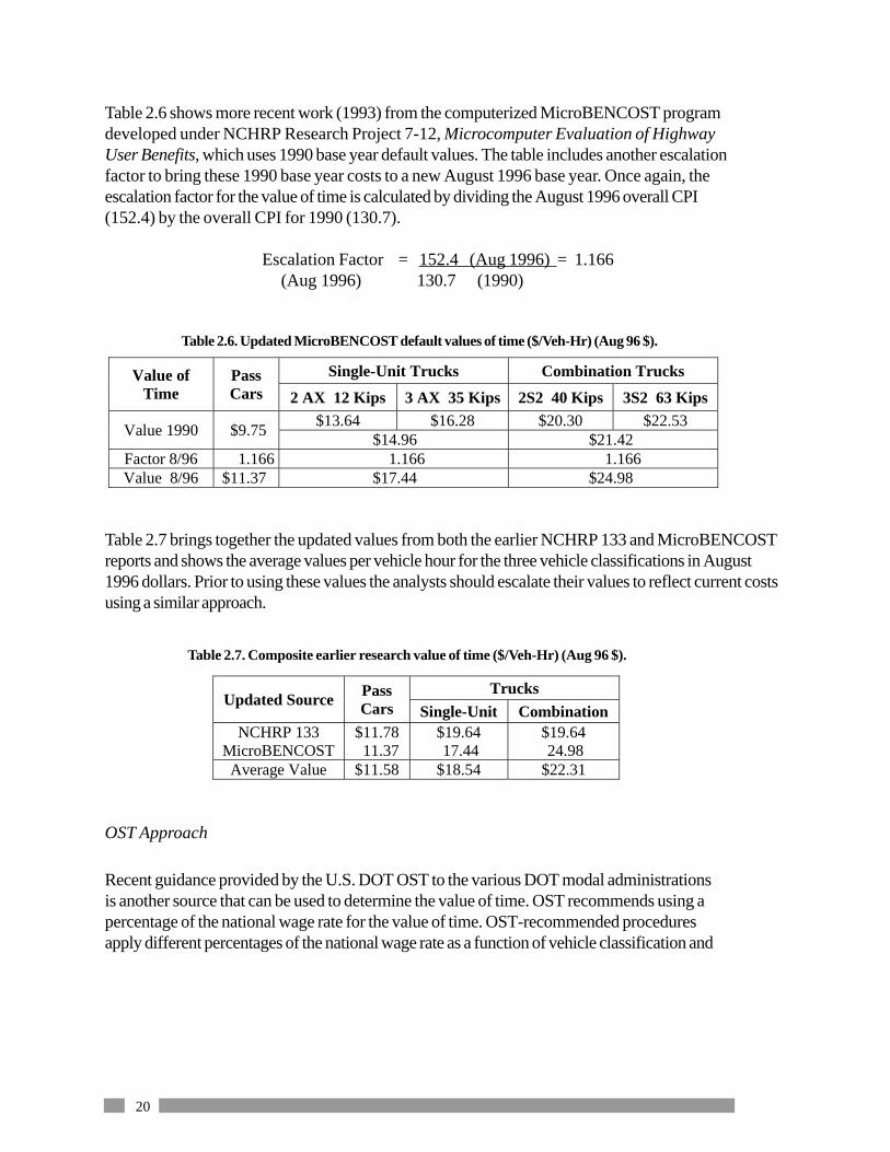
20

Table 2.6 shows more recent work (1993) from the computerized MicroBENCOST programdeveloped under NCHRP Research Project 7-12, Microcomputer Evaluation of HighwayUser Benefits, which uses 1990 base year default values. The table includes another escalationfactor to bring these 1990 base year costs to a new August 1996 base year. Once again, theescalation factor for the value of time is calculated by dividing the August 1996 overall CPI(152.4) by the overall CPI for 1990 (130.7).

Escalation Factor = 152.4 (Aug 1996) = 1.166 (Aug 1996) 130.7 (1990)

OST Approach

Recent guidance provided by the U.S. DOT OST to the various DOT modal administrationsis another source that can be used to determine the value of time. OST recommends using apercentage of the national wage rate for the value of time. OST-recommended proceduresapply different percentages of the national wage rate as a function of vehicle classification and

Table 2.7. Composite earlier research value of time ($/Veh-Hr) (Aug 96 $).

TrucksUpdated Source Pass

Cars Single-Unit CombinationNCHRP 133

MicroBENCOST$11.78 11.37

$19.64 17.44

$19.64 24.98

Average Value $11.58 $18.54 $22.31

Table 2.6. Updated MicroBENCOST default values of time ($/Veh-Hr) (Aug 96 $).

Single-Unit Trucks Combination TrucksValue ofTime

PassCars 2 AX 12 Kips 3 AX 35 Kips 2S2 40 Kips 3S2 63 Kips

$13.64 $16.28 $20.30 $22.53Value 1990 $9.75

$14.96 $21.42Factor 8/96 1.166 1.166 1.166Value 8/96 $11.37 $17.44 $24.98

Table 2.7 brings together the updated values from both the earlier NCHRP 133 and MicroBENCOSTreports and shows the average values per vehicle hour for the three vehicle classifications in August1996 dollars. Prior to using these values the analysts should escalate their values to reflect current costsusing a similar approach.

21

Table 2.9 provides information on national hourly wage rates used by OST in 1995 dollars.

Based on the information on appropriate percentages provided in table 2.8 and therecommended national hourly wage rate provided in table 2.9, the OST developed therecommended ranges for the value of travel time shown in table 2.10. The values associatedwith Mixed are the ranges to be used when the distribution between auto business and personaltrips is not known. Hourly values shown for trucks are $16.50 for both local and intercity triptypes.

Table 2.10 lists the ranges of values in dollars per person hour. As most user delay analysescompute vehicle hours of delay, these values must be adjusted for vehicle occupancy rates.

Trip TypeTravelCategory Local Intercity

Personal $17.00 $17.00Business 18.80 18.80Truck Drivers 16.50 16.50

Table 2.9. OST-recommended hourly wage rates (1995 $/Person-Hr).

U.S. DOT, The Value of Travel Time: Departmental Guidance forConducting Economic Evaluations.

Local IntercityTravelCategory Low High Low High

Personal $6.00 $10.20 $10.20 $15.30Business 15.00 22.60 15.00 22.60Mixed 6.40 10.70 10.40 15.70Truck Drivers 16.50 16.50 16.50 16.50

Table 2.10. Ranges for hourly values of travel time (1995 $/Person-Hr)

U.S. DOT, The Value of Travel Time: Departmental Guidance for ConductingEconomic Evaluations.

Table 2.8. Travel time ranges as a percent of national wage rate (1995 $/Person-Hr).

U.S. DOT, The Value of Travel Time: Departmental Guidance forConducting Economic Evaluations.

Trip TypeTravelCategory Local IntercityPersonal 35 to 60% 60 to 90%Business 80 to 120% 80 to 120%

Truck Drivers 100% 100%

trip type and purpose. Table 2.8 provides U.S. DOT ranges of the percentage of the nationalwage rate that should be applied to various combinations of trip type and purpose. The ratesshown are per person hour. As can be seen in table 2.8, business and truck travel are valuedmore highly than personal travel, and intercity personal travel is valued more highly than localpersonal travel.

22

According to the 1990 Personal Transportation Survey, typical auto vehicle occupancy ratesfor personal travel are 1.7 in urban areas and 2.0 in rural areas.(12) The typical vehicleoccupancy rates for trucks and auto business use is much closer to 1.0.

The values of travel time shown on lines 1 and 2 of table 2.11 are per vehicle hour based ontypical vehicle occupancy rates. The values associated with % AADT Personal Use on line 3represent the percent of travel that is personal. The Weighted Average values shown on line 4are for mixed flow of business and personal travel and are used when traffic flow distribution bytravel category is not known. The values shown for trucks are significantly higher than eitherearly research study or the OST guidance. Part of the higher cost (approximately 30 percent) isattributable to value associated with the vehicle cargo and the vehicle itself.

Toll Roads

Finally, another source that can be used to estimate the dollar values of time includes tolls on tollroads in relation to time saved. One of the more interesting revelations of users’ willingness topay comes from the treatment of some High Occupancy Vehicle (HOV) facilities in Californiaand Texas. Both States are experimenting with High Occupancy Toll (HOT) facilities, whichallow Single Occupancy Vehicles (SOV) to use an HOV facility for a fee. These studies dealprimarily with local auto trips and to some extent may reflect market prices. While the valuesinferred from such studies tend to indicate lower values of time (approximately $6 per personhour), they may in reality reflect inefficient pricing policy rather than lower values.

Table 2.11. Value of one vehicle hour of travel time (1995 $).

Autos Trucks

Single-Unit CombinationsTravel

Category Small Medium4 Tire 6 Tire 3-4 Axle 4 Axle 5 Axle

Business $27.99 $28.29 $20.20 $24.96 $27.02 $31.02 $31.58

Personal 12.78 $12.78 $12.78 NA NA NA NA% AADTPersonal Use

90% 90% 69% 0% 0% 0% 0%

WeightedAverage

$14.30 $14.33 $15.08 $24.96 $27.02 $31.02 $31.58

FHWA Highway Economic Requirements System Technical Report v3-1 9/97 (Exhibit 8-7).

FHWA Highway Economic Requirements System (HERS) Model

The FHWA uses the HERS Model in conducting national-level analysis of highwayperformance, needs, and economic evaluation of proposed highway improvements. Part of theeconomic analysis includes determining the value of travel time delay. Table 2.11 shows thedefault dollar values of travel time used in the HERS model.

23

Recommended Values of Travel Time (Dollars per Vehicle Hour)

Table 2.12 below is a composite table that brings together the several sources of the valueof time previously discussed.

TrucksPassenger Cars

Single-Unit Combinations$10 to 13 $17 to 20 $21 to 24

Table 2.13. Recommended values of time ($/Veh-Hr)(Aug 96 $).

Table 2.12. Composite listing of travel time values.

Source Units Autos Trucks Combination

U.S. DOT – OST * $/Person-Hr $10.80 $16.50 $16.50MicroBENCOST $/Veh-Hr 11.37 17.44 24.98NCHRP $/Veh-Hr 11.78 19.64 19.64HERS $/Veh-Hr 14.30 25.99 31.30

* Values for U.S. DOT — OST reflect dollars per person hour

Based on consideration of these potential sources, table 2.13 reflects the ranges of the valueof travel time per vehicle recommended for use in typical analyses where distribution dataon trip purpose and type are not known.

Crash Cost Rates

The MicroBENCOST software package, developed for the NCHRP Research Project 7-12, includes default crash cost rates. Table 2.14 shows the default crash cost rates by crashtype for both rural and urban settings in 1990 dollars.

Fatality NonfatalInjury

Property DamageOnly (PDO)Intersection or

Facility TypeRural Urban Rural Urban Rural Urban

RR Grade CrossingIntersection/InterchangeBridgeHighway Segment

$1,008 1,059 1,111 1,111

$994$932$978$978

$25.2 21.9 24.9 24.9

$13.3 14.3 14.3 14.3

$1.59 1.98 2.14 2.14

$3.09 1.35 1.27 1.27

Table 2.14. MicroBENCOST default crash cost rates ($1,000, 1990 $).

24

The MicroBENCOST 1990 dollar default values shown in table 2.14 are escalated to August1996 dollars in table 2.15 using the 1.116 escalation factor developed earlier.

The MicroBENCOST default cost values for a fatality range from $1,091,000 to $1,182,000,which is quite a bit lower than the $2,700,000 cost per fatality averted, which wasrecommended by the U.S. DOT in its March, 14, 1995 memorandum from the AssistantSecretary for Transportation Policy to DOT Modal Administrators. This $2,700,000 value is anupdate of the value originally recommended in basic guidance distributed on January 8, 1993.

In addition to the traditional direct work zone user costs, there are indirect user costs such asthe impact of user delay on delivery fleet size, the costs associated with a rolling inventory, andother, indirect effects of delay to manufacturing plants that now dependent on just-in-timedelivery. While such factors will become more important over time, they are beyond the scopeof these guidelines. It is interesting to note that cost related to delivery fleet size and the costsassociated with a rolling inventory are included in the dollar value of delay time rates used in theFHWA HERS Model.

DEVELOP EXPENDITURE STREAM DIAGRAMS

Expenditure stream diagrams are graphical representations of expenditures over time. They aregenerally developed for each pavement design strategy to help visualize the extent and timing ofexpenditures. Figure 2.4. shows a typical expenditure stream diagram.

Fatality Nonfatal Injury PDOIntersection orFacility Type Rural Urban Rural Urban Rural Urban

RR Grade CrossingIntersection/InterchangeBridgeHighway Segment

$1,125 1,182 1,240 1,240

$1,109 1,040 1,091 1,091

$28.1 24.4 27.8 27.8

$14.8 16.0 16.0 16.0

$1.77 2.21 2.39 2.39

$3.45 1.51 1.42 1.42

* Values for U.S. DOT-OST reflect dollars per person hour

Table 2.15. MicroBENCOST default crash cost rates ($1,000, Aug 96 $).

Figure 2.4. Typical expenditure stream diagram for a pavement design alternative.

Co

st (

$)

Rehabilitations

Salvage Value

InitialConstruction

Analysis Period

Time

25

∑

+ kni)1(

1

Normally, costs are depicted as upward arrows at the appropriate time they occur during theanalysis period, and benefits are represented as negative cost or downward arrows.

In LCC analysis of pavement design alternatives, the basic benefits of providing and maintainingsome preestablished pavement condition level on any given roadway are outside the scope ofthe analysis. The benefits of providing the specified level of pavement condition are consideredto be the same for all pavement design strategies. As a result, the only concerns are thedifferential costs among alternatives. The only negative cost (i.e., the only downward arrow)would be the cost associated with any salvage value.

Under these conditions, the LCCA objective becomes finding the alternative pavement designstrategy that meets the performance requirements at the lowest life-cycle cost.

COMPUTE NET PRESENT VALUE (NPV)

In its broadest sense, LCCA is a form of economic analysis used to evaluate the long-termeconomic efficiency between alternative investment options. Economic analysis focuses on therelationship between costs, timings of costs, and discount rates employed. Once all costs andtheir timing have been developed, future costs must be discounted to the base year and addedto the initial cost to determine the NPV for the LCCA alternative. As noted earlier, NPV is theeconomic indicator of choice, and the basic NPV formula for discounting discrete futureamounts at various points in time back to some base year is:

where: i = discount rate andn = year of expenditure

The component of the above formula is referred to as the Present Value (PV)

factor for a single future amount. PV factors for various combinations of discount rates andfuture years are available in Discount factor tables (more commonly referred to as interest ratetables). PV for a particular future amount is determined by multiplying the future amount by theappropriate PV factor. Table 2.16 shows discount factors for a single future payment at 3, 4,and 5 percent discount rates for up to 40 years in the future.

∑=

+

+=n

knk

kiNPV

1 )1(

1CostRehabCostInitial

N

26

Discount Factor Discount FactorYear 3% 4% 5% Year 3% 4% 5%

1 0.9709 0.9615 0.9524 21 0.5375 0.4388 0.35892 0.9426 0.9246 0.9070 22 0.5219 0.4220 0.34183 0.9151 0.8890 0.8638 23 0.5067 0.4057 0.32564 0.8885 0.8548 0.8227 24 0.4919 0.3901 0.31015 0.8626 0.8219 0.7835 25 0.4776 0.3751 0.29536 0.8375 0.7903 0.7462 26 0.4637 0.3607 0.28127 0.8131 0.7599 0.7107 27 0.4502 0.3468 0.26788 0.7894 0.7307 0.6768 28 0.4371 0.3335 0.25519 0.7664 0.7026 0.6446 29 0.4243 0.3207 0.242910 0.7441 0.6756 0.6139 30 0.4120 0.3083 0.231411 0.7224 0.6496 0.5847 31 0.4000 0.2965 0.220412 0.7014 0.6246 0.5568 32 0.3883 0.2851 0.209913 0.6810 0.6006 0.5303 33 0.3770 0.2741 0.199914 0.6611 0.5775 0.5051 34 0.3660 0.2636 0.190415 0.6419 0.5553 0.4810 35 0.3554 0.2534 0.181316 0.6232 0.5339 0.4581 36 0.3450 0.2437 0.172717 0.6050 0.5134 0.4363 37 0.3350 0.2343 0.164418 0.5874 0.4936 0.4155 38 0.3252 0.2253 0.156619 0.5703 0.4746 0.3957 39 0.3158 0.2166 0.149120 0.5537 0.4564 0.3769 40 0.3066 0.2083 0.1420

Table 2.16. Present value discount factors: single future payment.

Co

sts

($ 1

,000

)

$325Rehab. #1

Salvage Value $217

$1,100Initial Cost

Time (years)

$300User Cost

$269User Cost

$325Rehab. #2

$361User Cost

0 15 30 35

Figure 2.5. Expenditure stream diagram for agency and user costs.

NPV Computations

Example NPV computations are provided for the following hypothetical problem. The exampleis based on a 35-year analysis period.

The initial pavement design will cost $1.1 million and have an associated work zone user cost of$300,000 at year 0. Additional rehabilitation cost of $325,000 will be incurred in years 15 and30. Associated work zone user costs in years 15 and 30 will be $269,000 and $361,000,respectively. The salvage value at year 35, based on a prorated cost of the year-30rehabilitation design and remaining life, will be $216,000 (10/15 of $325,000). Figure 2.5shows the expenditure stream diagram for the example problem.

27

ANALYZE RESULTS

Once completed, all LCCA should, at a minimum, be subjected to a sensitivity analysis.Sensitivity analysis is a technique used to determine the influence of major LCAA inputassumptions, projections, and estimates on LCCA results. In a sensitivity analysis, major inputvalues are varied (either within some percentage of the initial value or over a range of values)while all other input values remain constant and the amount of change in results is noted. Theinput variables may then be ranked according to their effect on results. Sensitivity analysisallows the analyst to subjectively get a feel for the impact of the variability of individual inputson overall LCCA results.

Many times a sensitivity analysis will focus on best case/worst case scenarios in an attempt tobracket outcomes. Most LCC sensitivity analysis, as a minimum, evaluate the influence of thediscount rate used on LCCA results.

Note that estimated user costs drop in year 15 and go back up in year 30. This is consistentwith a longer duration initial work zone followed by short duration rehabilitation work zonesimpacted by continually increasing traffic volumes over time. Table 2.17 shows the results ofPV computations using 4 percent PV factors for single future amounts for the exampleexpenditure stream diagram. The bottom line of table 2.17 shows the NPV of the aggregatedindividual PVs.

Table 2.17. NPV calculation using 4 percent discount rate factors.

Cost Component Activity Years Costs($1,000)

DiscountFactor

DiscountedCost ($1,000)

Initial Construction 0 1,000.0 1.0000 1,000Initial Work Zone User Cost 0 300.0 1.0000 300Rehab #1 15 325.0 0.5553 180Rehab #1 Work Zone User Cost 15 269.0 0.5553 149Rehab #2 30 325.0 0.3083 100Rehab #2 Work Zone User Cost 30 361.0 0.3083 111Salvage Value 35 -216.6 0.2534 -55Total NPV 1,785

28

Sensitivity analyses may be carried out using common spreadsheet-based applications such asMicrosoft Excel, Lotus, or Quattro Pro. Tables 2.18 and 2.19 present the results of a spreadsheetanalysis of the sensitivity of NPV of two example pavement design strategies to discount rateranges from 2 to 6 percent for a 35-year analysis period. Total NPV at discount rates rangingfrom 2 to 6 percent are shown at the bottom of columns (e) through (i).

Table 2.18. Sensitivity analysis – Alternative #1.

Table 2.19. Sensitivity analysis – Alternative #2.

NPVActivity

(a)Year(b)

Cost(c)

2.0%(e)

3.0%(f)

4.0%(g)

5.0%(h)

6.0%(i)

Construction 0 1,100 1,100 1,100 1,100 1,100 1,100User Cost 0 300 300 300 300 300 300Rehab #1 15 325 241 209 180 156 136User Cost # 1 15 269 200 173 149 129 112Rehab # 2 30 325 179 134 100 75 57User Cost # 2 30 361 199 149 111 84 63Salvage 35 -217 -108 -77 -55 -39 -28

Total NPV 2,112 1,987 1,886 1,805 1,739

NPVActivity

(a)Year(b)

Cost(c)

2.0%(e)

3.0%(f)

4.0%(g)

5.0%(h)

6.0%(i)

Construction 0 975 975 975 975 975 975User Cost 0 200 200 200 200 200 200Rehab #1 10 200 164 149 135 123 112User Cost # 1 10 269 220 200 182 165 150Rehab # 2 20 200 135 111 91 75 62User Cost # 2 20 361 243 200 165 136 113Rehab # 3 30 200 110 82 62 46 35User Cost # 3 30 485 268 200 150 1,122 85Salvage 35 -100 -50 -36 -25 -18 -13

Total NPV 2,266 2,081 1,934 1,815 1,718

Alternative #1 has a lower initial agency cost, and, because of a shorter construction period, alower user cost than Alternative #2. However, Alternative #1 requires three identical 10-yeardesign rehabilitations compared to two identical 15-year design rehabilitations for Alternative #2.

Out-year user costs for Alternative #1 increase as a result of increased traffic levels over time;out-year user costs for Alternative #2 first decrease due to a shorter work zone period and thenincrease as a result of increased traffic levels over time.

29

Both alternatives have a remaining service life at year 35; Alternative #1 has 5 years andAlternative #2 has 10 years. The salvage value, as a prorated share of the last rehabilitation, is50 percent (5 years remaining on a 10-year design) of its last rehabilitation cost for Alternative#1. For Alternative #1, this translates into 50 percent of the $200,000 year-30 rehabilitationcost. The salvage value of Alternative #2, on the other hand, is 66.6 percent (10 yearsremaining on a 15-year design) of its last rehabilitation cost. This translates into 66.6 percent ofthe $325,000 year-30 rehabilitation cost.

Table 2.20 shows a direct comparison of the NPV of both alternatives at several discount rates.Inspection of table 2.20 reveals that the NPV of both alternatives decreases as the discountrate increases. This results from the reduced present value of future costs at higher discountrates. Because the amount and timing of future costs differ between alternatives, the effect ofdiscount rate on NPV is different for each alternative. In this example, Alternative #1 is more

Figure 2.6. Sensitivity of NPV to discount rate.

Table 2.20. Comparison of alternative NPVs ($1,000) to discount rate.

Discount Rate (%)Activity

2.0 3.0 4.0 5.0 6.0

Total NPV Alternative #1 2,266 2,081 1,934 1,815 1,718

Total NPV Alternative #2 2,112 1,987 1,886 1,805 1,739

Cost Advantage Alt #2 vs #1 154 94 48 10 -21

Sensitivity to Discount Rate

1,6001,7001,800

1,9002,0002,1002,200

2,3002,400

2.0% 3.0% 4.0% 5.0% 6.0%

Discount Rate

To

tal N

PV

Alt-1

Alt-2

expensive than Alternative #2 at discount rates of 5 percent and lower, while Alternative #2 ismore expensive than Alternative #1 at discount rates of 6 percent or more. Figure 2.6 showsthese results graphically.

30

Table 2.21. Sensitivity to user cost and discount rate.

Table 2.21 separates agency and user cost differences for the same range of discount rates.Inspection of the table 2.21 reveals that Alternative #2 has a higher agency cost than Alternative#1 at all discount rates considered. Further, Alternative #2 has lower user cost than Alternative#1 at all discount rates considered.

Discount Rate, %Cost Component

2.0 3.0 4.0 5.0 6.0Alternative #1 Agency CostAlternative #2 Agency Cost

1,3341,413

1,2811,366

1,2381,326

1,2011,292

1,1711,264

Agency Cost Advantage Alt #2 vs #1 -79 -85 -88 -91 -93

Alternative #1 User CostAlternative #2 User Cost

932699

800621

696561

613513

547475

User Cost Advantage Alt #2 vs #1 233 179 135 100 72Incremental Benefit/Cost (#2 vs #1) 2.95 2.11 1.53 1.10 0.77

The decision to include or exclude user costs can significantly affect the LCCA results. In aneffort to put the agency and user costs in perspective, the bottom row of table 2.21 includes anincremental B/C comparison of the reduction in user costs as a function of increased agencycosts. The incremental B/C data in table 2.21 is computed by dividing the reduction in usercosts (i.e., benefits) associated with selecting Alternative #2 in lieu of Alternative #1 by theadded agency cost(s) associated with selection of Alternative #2.

Similar sensitivity analyses could be conducted using other input variables such as agency cost,user costs, pavement performance lives, and hourly dollar value of user delay.

In addition to conducting a sensitivity analysis, the analyst should examine the implications ofcontractor work hours on queuing costs as well as the anticipated maximum queue lengths anddelay times. Chapter 3 details queue lengths and discusses associated user costs.

A primary drawback of the sensitivity analysis is that the analysis gives equal weight to any inputvalue assumptions, regardless of the likelihood of occurring. In other words, the extreme values(best case and worst case) are given the same likelihood of occurrence as the expected value—which is not realistic. Chapter 4 presents a powerful analytical technique to overcome thislimitation.

31

REEVALUATE DESIGN STRATEGY

Once the net present values have been computed for each alternative and limited sensitivityanalysis performed, the analyst needs to step back and reevaluate the competing designstrategies. As noted in chapter 1, the overall benefit of conducting a life-cycle cost analysis isnot necessarily the LCCA results themselves, but rather how the designer can use theinformation resulting from the analysis to modify the proposed alternatives and develop morecost-effective strategies.

For example, if user costs dwarf agency costs for all the alternatives, the analysis may indicatethat none of the alternatives analyzed are viable. It could indicate that the designer needs toevaluate the current design strategies’ impacts on future maintenance of traffic . . . that thedesign strategies should reflect the need for additional capacity in the out-years to mitigate theimpact on highway users. The solution to out-year capacity problems could include enhancedstructural design of the shoulders in early-year pavement designs to allow for the use of theshoulder in subsequent rehabilitation traffic control plans. It also could include enhancedstructural design of the mainline pavement to minimize the frequency of subsequent rehabilitationefforts and designing in features that will make future rehabilitation proceed more smoothly.Other options available include revising the maintenance of traffic plans, reducing theconstruction period, restricting the contractor’s work hours or imposing lane rental fees,planning for additional lanes/routes, and even examining programs to temporarily shift traffic toalternative modes of travel. It is important to note that restricting the contractor’s hours ofoperation or the number of work days allowed will more than likely increase agency cost.

LCCA results are just one of many factors that influence the ultimate selection of a pavementdesign strategy. The final decision may include a number of additional factors outside the LCCAprocess, such as local politics, availability of funding, industry capability to perform the requiredconstruction, and agency experience with a particular pavement type, as well as the accuracy ofthe pavement design and rehabilitation models. Chapter 3 of the 1993 AASHTO PavementDesign Guide further discusses such other factors.(13) When such other factors weigh heavilyin the final pavement design selection, it is imperative to document their influence on the finaldecision.

Many assumptions, estimates, and projections feed the LCCA process. The variabilityassociated with these inputs can have a major influence on the confidence the analyst can placein LCCA results. It all depends on the accuracy of the inputs used. The accuracy of LCCAresults depends directly on the analyst’s ability to accurately forecast such variables as futurecosts, pavement performance, and traffic for more than 30 years into the future. To effectivelydeal with the uncertainty associated with such forecasts, a probabilistic risk analysis approach(as presented in chapter 4) is increasingly essential to quantitatively capture the uncertaintyassociated with input parameters in LCCA results.

32

33

This chapter presents a rational, step-by-step procedure to allow the analyst, based on capacityflow analysis, to determine user costs associated with establishing a work zone. Chapter 2discussed user cost rates. This chapter focuses on calculating the quantity associated with eachof the individual user cost components (VOC, user delay, and crashes) and computing overalluser costs in a spreadsheet environment. The chapter ends with a discussion of automatedcomputer programs.

While there are microcomputer-based user cost analysis software programs currently available,it is important that the analyst thoroughly understand the principles involved before attempting toapply them. By understanding the major factors influencing work zone user costs, the analystcan take steps to minimize the effect of planned future rehabilitation activities on highway users.

WORK ZONE USER COSTS

Work zone user costs are the increased VOC, delay, and crash costs to highway users resultingfrom construction, maintenance, or rehabilitation work zones. They are a function of the timing,duration, frequency, scope, and characteristics of the work zone; the volume and operatingcharacteristics of the traffic affected; and the dollar cost rates assigned to vehicle operating,delay, and crashes. The following sections address each of these issues.

In the end, user costs are computed by multiplying the quantity of additional VOC, delay, andnumber of crashes by the unit cost rates assigned to these components.

WORK ZONE DEFINED

Work Zone is defined in the Highway Capacity Manual (HCM) as an area of a highwaywhere maintenance and construction operations impinge on the number of lanes available totraffic or affect the operational characteristics of traffic flowing through the area.(14)

Each work zone established over the analysis period affects traffic flow and associated usercosts differently and must be evaluated as a separate event. A separate work zone must bedefined and analyzed whenever characteristics of the work zone or the characteristics of theaffected traffic change.

Pavement design performance differences directly affect the frequency and timing ofmaintenance and rehabilitation activities. Pavement rehabilitation and maintenance activitiesgenerally occur at different points in the analysis period with different traffic, and they generallyvary in scope and duration. The time that they occur also affects the influence of the discountfactor used in developing NPV.

CHAPTER 3. WORK ZONE USER COSTS

34

WORK ZONE CHARACTERISTICS

In order to analyze work zone user costs, work zone characteristics associated with alternativedesigns and supporting maintenance and rehabilitation strategies must be defined as part of thedevelopment of alternative pavement design strategies. Alternative pavement preservationstrategies must include how often (the number of times) the facility will be under construction,maintenance or rehabilitation activities, and the year at which work zones are anticipated.Strategies should also include estimates of the number of days the work zone will last, the hoursof the day the work zone will be in place, and the anticipated maintenance of traffic strategy.

Work zone characteristics of concern include such factors as work zone length, number andcapacity of lanes open, duration of lane closures, timing (hours of the day, days of the week,season of the year, etc.) of lane closures, posted speed, and the availability and physical andtraffic characteristics of alternative routes. The strategy for maintaining traffic should include anyanticipated restrictions on contractor’s or maintenance force’s hours of operations or ability toestablish lane closures. Specific details in an LCCA should include:

� Projected year work zones occur (years 5, 8, 12, etc,).

� Number of days the work zone will be in place (construction period).

� Specific hours of each day, as well as the days of the week the work zone will be inplace.

� Work zone length and posted speed.

The duration of a work zone (the overall length of time a facility or portion of a facility is out ofservice or traffic is restricted) can range from sporadic daily lane closures for maintenance toseveral months for bridge deck replacements.

As noted earlier, the differential routine maintenance cost between alternative pavement designstrategies tends to be insignificant when compared to initial construction and rehabilitation costs.To a great extent, the same is true of user costs resulting from routine reactive-type maintenanceactivities. Routine maintenance work zones tend to be relatively infrequent, of short duration,and outside of peak traffic flow periods. As such, analysts should focus attention on user costsassociated with major work zones.

TRAFFIC CHARACTERISTICS

User costs are directly dependent on the volume and operating characteristics of the traffic onthe facility. Each construction, maintenance, and rehabilitation activity generally involves sometemporary effect on traffic using the facility. The effect can vary from insignificant for minor workzone restrictions on low-volume facilities to highly significant for major lane closures on high-volume facilities.

35

The major traffic characteristics of interest for each year a work zone will be established include:(1) the overall projected Average Annual Daily Traffic (AADT) volumes on both the facility andpossibly alternate routes, (2) the associated 24-hour directional hourly demand distributions,and (3) the vehicle classification distribution of the projected traffic streams. On high-volumeroutes, distinctions between weekday and weekend traffic demand and hourly distributionsbecome important. Further, seasonal AADT traffic distribution also becomes important whenwork zones are proposed on recreational routes during seasonal peak periods.

AADT

Current AADT volumes are normally readily available for the base year and projectedcompound traffic growth rates can be obtained from the SHA traffic monitoring section. Fromthese two pieces of information, calculating future year work zone AADT is relatively simple.

While the calculations for future year AADT are rather straightforward, there are two majorissues associated with the reasonableness of such projections on high-volume urban facilities.The first is whether the roadway in question can handle large projected volume increases; thesecond is whether traffic using a facility will continue to use it when work zones are establishedand traffic flow is restricted.

In the first issue, design capacity and ultimate capacity are quite different. Design capacity isgenerally set to handle the design year 30 highest hour volume at level of service D or E.However, table 2.1 of the HCM shows measured maximum 24-hour traffic volumes for some ofthe more heavily traveled interstate urban freeways that far exceed the traffic volumes normallyassociated with level of service D or E. Reasonableness dictates that AADT projections shouldnot exceed the maximum observed 24-hour traffic volumes contained in table 2.1 of the HCM.

The next section discusses the second issue, which relates to whether traffic using a facility willcontinue to use it when work zones are established and traffic flow is restricted.

Traffic Diversion

Traffic demand is generally determined based on facility operating characteristics during periodsof normal operations. Traffic demand during work zone operations may or may not be the same.Some portion of the traffic normally wanting to use the facility may divert to other routes whenwork zones are established.

Vehicles use a given facility because it offers what the vehicle operators perceive as the leastexpensive combination of vehicle operating and time delay costs, consistent with safetyrequirements. When faced with restricted flow, or even the anticipation of restricted flow,vehicle operators who normally use a facility will exercise one of several options, which aresomewhat whimsically categorized below.

Hang Toughers will continue to use the facility as they always have. They are primarily userswith little or no option. They (1) must make the trip; (2) must make it at a specific time; and (3)

36

either don’t know or don’t have alternative routes or modes from which to choose. These userspay the full price of the work zone and have little effect on other facilities in the corridor. In ruralareas the predominate choice of through traffic will be to tough it out, as these users generallymust make the trip and do not have much information on alternative routes unless formal detoursare established.

Time Shifters have the ability and choose to travel on the facility at a different time — generallya time well outside of the restricted flow period. These users lessen their impact by sharing theimpact with other vehicles by invading their time slot. These users also have little effect on otherhighway facilities in the corridor, but they do affect hourly traffic distribution.

Detourees either seek out and use alternate routes or are forced to negotiate detoursestablished by the highway agency. These operators also lessen their impact by sharing theimpact with other vehicles by invading their routes. They tend to trade off anticipated timedelay for additional travel distances and associated vehicle operating costs. In urban areas thiscould include users who switch modes. Detourees can have significant impact on overall usercosts of alternative routes, especially those operating at or near capacity. The sections onCircuitry (page 69) and Crash Costs (page 70) address the additional user costs associatedwith the additional mileage traveled by detoured and diverted traffic.

Trip Swappers have the luxury of totally abandoning the trip or seeking other destinations whenthe cost, in terms of time and money, becomes too great. Historically, this group consistsprimarily of shopping and social/recreational trip makers. While their behavior may diminish theuser cost impact of the work zone, they adversely affect businesses along the route in question.More recent trends in people working out of the home and telecommuting may significantlyaffect work trips in the future.

Handling Diversion

In simple cases, where either work zone disruption is tolerable or alternative routes are limited,estimated AADT during the year of the work zone can be anticipated to continue on the facilityand the work zone analysis can be limited to the existing facility.

In more complex situations where existing traffic would face intolerable work zone disruptions, itis entirely possible that total travel demand and hourly distribution on the facility may changewhen the work zone is established. When demand changes, the scope of work zone user costanalysis may have to expand beyond the existing facility and include user cost changes on majoralternative routes. When preliminary analysis of travel demand shows that work zone userdelays are unreasonably high, the analyst should seek special help from the traffic engineeringsection to generate revised traffic demand forecasts during work zone operations.

An alternative approach is to assume that those extraordinary user costs are truly there, andtime and route shifters are merely diminishing their effect by sharing the costs with users of otherroutes and time slots. In short, the misery’s still there — it’s just being shared differently.

37

Vehicle Classification

Highway user costs are a composite of the costs of all affected highway users. Highway usersare not a homogeneous group. They include commercial and noncommercial vehicles rangingfrom passenger vehicles through the heaviest trucks. These different vehicle types have differentoperating characteristics and associated operating costs. Further, the value of user delay differsbetween vehicle classes. As a result, user costs need to be analyzed for each major vehicle classpresent in the traffic stream.

There are many truck-vehicle classifications representing various size and weight configurations.Appendix A of the FHWA Traffic Monitoring Guide, includes 13 different vehicleclassifications.

(15) User cost analysis based on 13 vehicle classes is much too detailed for the

level of sophistication in the analysis procedures presented.

A more reasonable approach is to use three broad vehicle classes:

1. Passenger cars and other 2-axle, 4-tired passenger vehicles (classification types 1-3)

2. Single-unit trucks, 2-axle, 4-tired or more commercial trucks (classification types 4-7)

3. Combination-unit trucks (classification types 8-13)

On high traffic volume facilities, user delay costs are likely to represent a very significantcomponent of overall user costs in a pavement design LCCA, particularly when vehicle demandexceeds capacity. As passenger vehicles represent the bulk of vehicles in the traffic stream,analysts may find it beneficial to subdivide passenger vehicles into commercial andnoncommercial categories. Further, although vehicle occupancy rates have consistently fallenover time, they cannot generally be ignored.

Directional Hourly Traffic Distribution

The estimated hourly traffic distribution during work zone operations is essential to compare theunrestricted demand on the facility with the facility’s ability to carry that traffic through the workzone. Hourly distribution specific to a particular facility can be developed from agency trafficdata or general distribution data developed for various functional class- and area-typecombinations. On high-volume or tourist destination routes, the difference between weekdayand weekend traffic volumes and hourly distributions needs to be considered.

Table 3.1 represents default directional hourly distributions for Urban and Rural roadwaysincluded in MicroBENCOST. The table also includes hourly directional distribution factorsassociated with inbound and outbound directions. The hourly demand is computed bymultiplying the AADT by the hourly percent and directional factors for the direction in question.

Hourly Demand = AADT x Hourly Distribution Factor x Hourly Directional Factor

38

For example, the inbound directional hourly demand volume between 8 and 9 a.m. on an urbanroadway with a 40,000 AADT would be:

40,000 AADT x 6.3% x 59% = 1,487 vehicles/hour

Although MicroBENCOST provides for the use of different directional hourly distributionvalues for Interstate, Principal Arterial, Minor Arterial, and Major Collector, the default

Table 3. 1. Default hourly distributions from MicroBENCOST (all functional classes).

Rural Urban

Direction % Direction %Hour

(24-HrClock)

%ADT In Out

%ADT In Out

0 – 1 1.8 48 52 1.2 47 53

1 – 2 1.5 48 52 0.8 43 57

2 – 3 1.3 45 55 0.7 46 54

3 – 4 1.3 53 47 0.5 48 52

4 – 5 1.5 53 47 0.7 57 43

5 – 6 1.8 53 47 1.7 58 42

6 – 7 2.5 57 43 5.1 63 37

7 – 8 3.5 56 44 7.8 60 40

8 – 9 4.2 56 44 6.3 59 41

9 – 10 5.0 54 46 5.2 55 45

10 – 11 5.4 51 49 4.7 46 54

11 – 12 5.6 51 49 5.3 49 51

12 – 13 5.7 50 50 5.6 50 50

13 – 14 6.4 52 48 5.7 50 50

14 – 15 6.8 51 49 5.9 49 51

15 – 16 7.3 53 47 6.5 46 54

16 – 17 9.3 49 51 7.9 45 55

17 – 18 7.0 43 57 8.5 40 60

18 – 19 5.5 47 53 5.9 46 54

19 – 20 4.7 47 53 3.9 48 52

20 – 21 3.8 46 54 3.3 47 53

21 – 22 3.2 48 52 2.8 47 53

22 – 23 2.6 48 52 2.3 48 52

23 – 24 2.3 47 53 1.7 45 55

39

values listed are the same for all functional classes. Pennsylvania, on the other hand, providesdifferent hourly distributions for various functional class roadways, but it does not provide adirectional split factor. Table 3.2 contains statewide hourly distribution factors used byPennDOT in developing user delay cost.

CONCEPTUAL ANALYSIS

Before addressing user cost calculation procedures, it is helpful to conduct a conceptual analysisof a work zone operation. There are seven possible work zone user cost components that canoccur; three are associated with a Base Case situation where traffic operates under Free-Flowconditions, and four are associated with a Queue situation where traffic operates under Forced-Flow conditions. The next section conceptually discusses potential user costs involved underFree-Flow and Forced-Flow (Level of Service F) conditions.

Free Flow

Work zones restrict traffic flow either by reducing capacity or, as a minimum, by posting lowerspeed limits. Figure 3.1 shows free-flow conditions at a work zone. All traffic that flows through

Table 3.2. PennDOT AADT distribution (hourly percentages).

Hour (24 Hr

Clock) Urban Rural Urban Rural Urban Rural12 – 1 1.3 1.7 0.9 0.9 0.8 0.71 – 2 0.9 1.4 0.5 0.5 0.4 0.42 – 3 0.8 1.3 0.4 0.5 0.3 0.33 – 4 0.8 1.3 0.4 0.5 0.3 0.44 – 5 1.1 1.4 0.6 0.9 0.4 0.85 – 6 2.1 2.1 1.8 2.3 1.3 2.26 – 7 4.7 3.7 4.4 4.9 4.0 4.57 – 8 6.4 4.9 6.2 6.2 6.4 5.58 – 9 5.6 4.9 5.7 5.5 5.7 5.39 – 10 5.1 5.2 5.1 5.3 4.8 5.4

10 – 11 5.2 5.5 5.2 5.4 4.9 5.811 – 12 5.4 5.8 5.6 5.6 5.5 6.012 – 13 5.5 5.7 6.0 5.7 6.0 6.213 – 14 5.5 5.9 5.9 5.9 5.7 6.414 – 15 6.1 6.3 6.4 6.6 6.3 7.215 – 16 7.3 6.9 7.4 7.7 7.6 8.116 – 17 7.8 7.2 7.8 8.0 8.3 8.017 – 18 7.2 6.6 7.5 7.4 8.0 7.118 – 19 5.4 5.3 5.9 5.5 6.2 5.419 – 20 4.3 4.4 4.8 4.3 5.1 4.420 – 21 3.7 3.8 4.0 3.6 4.3 3.621 – 22 3.2 3.4 3.3 3.0 3.4 2.922 – 23 2.6 2.9 2.4 2.3 2.4 2.123 – 24 2.0 2.4 1.7 1.5 1.6 1.4

Traffic Pattern GroupInterstate Principal Arterial Minor Arterial

40

the work zone must, at a minimum, slow while traveling through it and then accelerate back tonormal operating speed. This is commonly referred to as a speed change and it results in threework zone-related User Cost components: speed change delay, speed change VOC, andreduced speed delay. Figure 3.1 presents the cost components associated with free flow.

Speed Change Delay is the additional time necessary to decelerate from the upstreamapproach speed to the work zone speed and then to accelerate back to the initial approachspeed after traversing the work zone.

Speed Change VOC is the additional vehicle operating cost associated with decelerating fromthe upstream approach speed to the work zone speed and then accelerating back to theapproach speed after leaving the work zone.

Reduced Speed Delay is the additional time necessary to traverse the work zone at the lowerposted speed; it depends on the upstream and work zone speed differential and length of thework zone.

If traffic demand remains below work zone capacity, added work zone user costs are limited tothe above three components and the analysis is relatively simple. In most cases, delay timesremain relatively low and represent more of a minor irritation and inconvenience than a seriousproblem.

Construction ZoneConstruction ZoneConstruction ZoneShoulder

Free Flow

Speed Change VOCSpeed Change Delay

Reduced Speed Delay

Traverse Work

Figure 3.1. Free-flow cost components.

41

Once a queue develops, all approaching vehicles must not only slow down before proceedingthrough the work zone itself, but they also must stop at the upstream end of the queue andcreep through the length of the physical queue under forced-flow conditions. As long asdemand exceeds capacity, the length of the queue grows, exacerbating the problem. Whendemand eventually falls below capacity, or when capacity is increased above demand byremoving the work zone restriction, vehicles then leave the queue faster than they arrive and thelength of the queue shrinks and eventually dissipates. When capacity is reduced on high-trafficfacilities, it is common for queues to develop in the morning peak traffic period, dissipate, andthen redevelop in the afternoon peak traffic period. In exceptionally congested areas, queuesmay form early in the morning and continue throughout the day and into the evening hours.

Queuing situations impose four work zone-related user costs that only apply to vehicles thatencounter a physical queue.

Stopping Delay is the additional time necessary to come to a complete stop from the upstreamapproach speed (instead of just slowing to the work zone speed) and the additional time toaccelerate back to the approach speed after traversing the work zone.

Stopping VOC is the additional vehicle operating cost associated with stopping from theupstream approach speed and accelerating back up to the approach speed after traversingwork zone.

Figure 3.2. Forced-flow cost components level of service F.

Upstream Queue Area Work Zone

Work Zone

Shoulder

Forced FlowForced Flow

Speed ChangeVOC & Delay

StoppingVOC & Delay

QueueIdling & Delay

Reduced Speed Delay(Traverse Work Zone)

Forced Flow (Level of Service F)

When hourly traffic demand exceeds work zone capacity, traffic flow breaks down and a queueof vehicles develops, as figure 3.2 shows. It is important to note that the queue forms not in thework zone itself, but in the upstream approach to the work zone.

42

Queue Delay is the additional time necessary to creep through the queue under forced-flowconditions.

Idling VOC is the additional vehicle operating cost associated with stop-and-go driving in thequeue. The idling cost rate multiplied by the additional time spent in the queue is anapproximation of actual VOC associated with stop-and-go conditions. When a queue exists,stopping delay and VOC replace the free-flow speed change delay and VOC.

The conceptual analysis presented here is geared primarily to freeway conditions. Conceptualanalysis of other facilities with at-grade intersections would also incur speed change, stopping,delay, and idling cost but at a much higher frequency, because of intersection-control devicesand turning movements.

COMPUTATIONAL ANALYSIS

Once the individual work zones have been identified, each is evaluated separately. This is thepoint at which individual user cost components are quantified and converted to dollar costvalues. This section provides an approach for actually quantifying and costing the individualwork zone user cost components encountered. The 12 overall steps involved are:

1. Project future year traffic demand.2. Calculate work zone directional hourly demand.3. Determine roadway capacity.4. Identify the user cost components.5. Quantify traffic affected by each component.6. Compute reduced speed delay.7. Select and assign VOC cost rates.8. Select and assign delay cost rates.9. Assign traffic to vehicle classes.10. Compute individual user costs components by vehicle class.11. Sum total work zone user costs.12. Address circuitry and crash costs.

Example Work Zone Problem Defined

The following information describes the work zone used as the example problem throughout theremainder of this section to illustrate the work zone user cost computational steps describedabove.

Facility: 3-lane directional outbound Interstate. Posted speed is 55 mi/h and grades onthe facility are less than 2 percent.

Traffic: Base year (1995) AADT of 122,000 vehicles per day. Vehicle classification counts indicate a traffic stream mix of 90 percent Passenger

43

Vehicles, 5.4 percent Single-Unit Trucks, and 4.6 percent Combination Trucks.The 10-year projected traffic growth rates for the various vehicle classificationsare 2.2 percent for passenger vehicles and 5 percent per year for both single-unit and combination trucks.

Work Zone: 5.25-mile-long single-lane closure from 9 a.m. until 3 p.m. and from 8 p.m. until5 a.m. the following morning. Work zone posted speed is 40 mi/h. The workzone will be in place for 60 days in 1999.

Step 1. Project Future Year Traffic Demand

The first step is to project future year hourly traffic demand volumes for each vehicle class forthe year the work zones will be in place, from current or base year AADT, using compoundtraffic growth factors. The following formula applies:

Future Year AADT = Base Year AADT x Vehicle class % x (1 + growth rate)(Future Yr. – Base Yr.)

The AADT on a facility in 1999 can be determined from a 1995 base year AADT of 122,000using the above formula by applying the appropriate compound growth rate factor (in thisexample 2.2 percent for passenger vehicles and 5 percent for trucks) as follows:

Projected 1999 AADT

Passenger Vehicles 122,000 x 0.900 x 1.022(4) = 109,800 x 1.09095 = 119,786 = 89%Single-Unit Trucks 122,000 x 0.054 x 1.050(4) = 6,588 x 1.21551 = 8,008 = 6%Combination Trucks 122,000 x 0.046 x 1.050(4) = 5,612 x 1.21551 = 6,821 = 5%Total Traffic 134,615 = 100%

Based on these new numbers, total traffic in 1999 will be 134,615, and because of thedifferential traffic growth rates for trucks, the 1999 vehicle mix will be approximately 89 percentfor passenger vehicles, 6 percent for single-unit trucks, and 5 percent for combination trucks.

Step 2. Calculate Work Zone Directional Hourly Demand

Directional hourly traffic distribution should be determined from agency traffic data on theroadway being analyzed or from traffic data on similar facilities. If, however, such data is notavailable, the default hourly distributions for various roadway types in urban and rural settingsfrom MicroBENCOST (reproduced in table 3.1) can be used. Table 3.3 contains the futureyear directional hourly demand for the example problem generated using the defaultMicroBENCOST urban outbound hourly distribution factors and 134,615 future year AADT.

44

Inspection of table 3.3 reveals that a.m. outbound demand peaks at 4,200 vehicles per hour inthe 7 to 8 a.m. period, while the p.m. outbound demand peaks at 6,885 vehicles per hour in the5 to 6 p.m. time period.

Table 3.3. Work zone directional hourly demand (all vehicle classes).

Step 3. Determine Roadway Capacity

In analyzing work zone user costs, there are three capacities that need to be determined: (1) the free-flow capacity of the facility under normal operating condition, (2) the capacity of the facility when thework zone is in place, and (3) the capacity of the facility to dissipate traffic from a standing queue.

Outbound Urban InterstateAADT134,615

(24-HrClock)

% ADT DirectionalFactor % Demand

12 – 1 1.2 53 8561 – 2 0.8 57 6142 – 3 0.7 54 5093 – 4 0.5 52 3504 – 5 0.7 43 4055 – 6 1.7 42 9616 – 7 5.1 37 2,5407 – 8 7.8 40 4,2008 – 9 6.3 41 3,4779 –10 5.2 45 3,15010 –11 4.7 54 3,41711 –12 5.3 51 3,63912 –13 5.6 50 3,76913 –14 5.7 50 3,83714 –15 5.9 51 4,05115 –16 6.5 54 4,72516 –17 7.9 55 5,84917 –18 8.5 60 6,86518 –19 5.9 54 4,28919 –20 3.9 52 2,73020 –21 3.3 53 2,35421 –22 2.8 53 1,99822 –23 2.3 52 1,61023–24 1.7 55 1,259

Total 67,453

45

Free-Flow Capacity is the maximum capacity a facility can handle under free-flow conditions.According to the 1994 HCM (p. 2-10), the maximum capacity for a 2-lane directional freewayunder ideal conditions is 2,200 passenger cars per hour per lane (pcphpl) and 2,300 pcphpl fora 3- or more lane directional freeway. The 1994 HCM points out the need to reduce the aboveideal condition capacities for such real world factors as restricted lane widths, reduced lateralclearances, the presence of trucks and recreational vehicles, and the presence of a driverpopulation unfamiliar with the area (p. 3-11). The real-world free-flow capacity of the facility isdetermined by applying the following formula:

Sfi = MSF

i x N x f

w x f

HV x f

p

SFi = service flow rate for LOS i under prevailing roadway and traffic conditions for N lanes in one direction in vehicles per hour (vph),

MSFi = Maximum service flow rate for LOS i for N lanes in one direction (vph)N = number of lanes in one direction of the freeway,fw

= factor to adjust for the effects of restricted lane widths and lateral clearances,fHV

= factor to adjust for the effect of heavy vehicles on the traffic stream, andfp

= factor to adjust for the effect of recreational or unfamiliar driver populations.

The following discussion describes the procedures to adjust maximum freeway capacity in termsof pcplph to real-world mixed vehicle conditions when there are trucks in the traffic stream (themost commonly encountered condition). For adjustments resulting from restricted lane width,reduced lateral clearance, and other adjustment factors when the work zone is not in place,refer to chapter 3 (p. 3-12) of the 1994 HCM.

The capacity adjustment resulting from the presence of trucks is based on the fact that trucksare larger than passenger vehicles and thus physically occupy more roadway space. Further,trucks, particularly when fully loaded, tend to be less nimble and maneuverable than passengervehicles, especially on long, steep up grades.

Truck equivalency factors are used to adjust highway capacity for the presence of trucks in thetraffic stream. Truck equivalency factors are a function of the percent trucks in the traffic streamand the degree and length of the maximum vertical grade on the facility. Table 3.4 reproducesthe truck equivalency factors for various combinations of percent trucks, grades, and gradelengths found in table 3-4 of the 1994 HCM.

Inspection of table 3.4 clearly shows that truck equivalency factors increase as grades andgrade length increase. The effect of grade and grade length diminishes as the percent of trucks inthe traffic stream increases. It is also clear from table 3.4 that at grades of less than 2 percent,the truck equivalency factor is 1.5, regardless of the length of the grade or the percent of trucksin the traffic stream. Because the example problem used throughout this chapter has bydefinition less than 2 percent grades, the truck equivalency factor for the example problem willbe 1.5.

46

Table 3.4. Truck equivalency factors.

Grade Length Percent Trucks and Buses% (Miles) 2 4 5 6 8 10 15 20 25< 2 All 1.5 1.5 1.5 1.5 1.5 1.5 1.5 1.5 1.5

0.00 - 0.25 1.5 1.5 1.5 1.5 1.5 1.5 1.5 1.5 1.5

0.25 - 0.50 1.5 1.5 1.5 1.5 1.5 1.5 1.5 1.5 1.5

2 0.50 - 0.75 1.5 1.5 1.5 1.5 1.5 1.5 1.5 1.5 1.5

0.75 - 1.00 2.5 2.0 2.0 2.0 1.5 1.5 1.5 1.5 1.5

1.00 - 1.50 4.0 3.0 3.0 3.0 2.5 2.5 2.0 2.0 2.0

> 1.50 4.5 3.5 3.0 3.0 2.5 2.5 2.0 2.0 2.0

0.00 - 0.25 1.5 1.5 1.5 1.5 1.5 1.5 1.5 1.5 1.5

0.25 - 0.50 3.0 2.5 2.5 2.0 2.0 2.0 2.0 1.5 1.5

3 0.50 - 0.75 6.0 4.0 4.0 3.5 3.5 3.0 2.5 2.5 2.0

0.75 - 1.00 7.5 5.5 5.0 4.5 4.0 4.0 3.5 3.0 3.0

1.00 - 1.50 8.0 6.0 5.5 5.0 4.5 4.0 4.0 3.5 3.0

> 1.50 8.5 6.0 5.5 5.0 4.5 4.5 4.0 3.5 3.0

0.00 - 0.25 1.5 1.5 1.5 1.5 1.5 1.5 1.5 1.5 1.5

0.25 - 0.50 5.5 4.0 4.0 3.5 3.0 3.0 3.0 2.5 2.5

4 0.50 - 0.75 9.5 7.0 6.5 6.0 5.5 5.0 4.5 4.0 3.5

0.75 - 1.00 10.5 8.0 7.0 6.5 6.0 5.5 5.0 4.5 4.0

>1.00 11.0 8.0 7.5 7.0 6.0 6.0 5.0 5.0 4.5

0.00 - 0.25 2.0 2.0 1.5 1.5 1.5 1.5 1.5 1.5 1.5

0.25 - 0.33 6.0 4.5 4.0 4.0 3.5 3.0 3.0 2.5 2.0

5 0.33 - 0.50 9.0 7.0 6.0 6.0 5.5 5.0 4.5 4.0 3.5

0.50 - 0.75 12.5 9.0 8.5 8.0 7.0 7.0 6.0 6.0 5.0

0.75 - 1.00 13.0 9.5 9.0 8.0 7.5 7.0 6.5 6.0 5.5

> 1.00 13.0 9.5 9.0 8.0 7.5 7.0 6.5 6.0 5.5

0.00 - 0.25 4.5 3.5 3.0 3.0 3.0 2.5 2.5 2.0 2.0

0.25 - 0.33 9.0 6.5 6.0 6.0 5.0 5.0 4.0 3.5 3.0

6 0.33 - 0.50 12.5 9.5 8.5 8.0 7.0 6.5 6.0 6.0 5.5

0.50 - 0.75 15.0 11.0 10.0 9.5 9.0 8.5 8.0 7.5 6.5

0.75 - 1.00 15.0 11.0 10.0 9.5 9.0 8.5 8.0 7.5 6.5

> 1.00 15.0 11.0 10.0 9.5 9.0 8.5 8.0 7.5 6.5

Tables 3.5 and 3.6 are maximum freeway capacity (mixed vehicles per lane per hour) look uptables based on truck equivalency factor and percent trucks in the traffic stream. Table 3.5 is for2-lane directional freeways and table 3.6 is for 3- or more lane directional freeways. Table 3.6 isthe appropriate table for the example problem. Table 3.6 (6- or more lane facility), with a truckequivalency factor of 1.5 and future year percent trucks of 11 percent, reveals by extrapolation afree-flow capacity of 2,180 vehicles per lane per hour, or 6,540 vph for all 3 lanes.

47

% Truck Equivalency FactorTrucks 1.5 2.0 2.5 3.0 3.5 4.0 4.5 5.0 5.5 6.00.0% 2,200 2,200 2,200 2,200 2,200 2,200 2,200 2,200 2,200 2,2002.0% 2,178 2,157 2,136 2,115 2,095 2,075 2,056 2,037 2,018 2,0004.0% 2,157 2,115 2,075 2,037 2,000 1,964 1,930 1,897 1,864 1,8335.0% 2,146 2,095 2,047 2,000 1,956 1,913 1,872 1,833 1,796 1,7606.0% 2,136 2,075 2,018 1,964 1,913 1,864 1,818 1,774 1,732 1,6928.0% 2,115 2,037 1,964 1,897 1,833 1,774 1,719 1,667 1,618 1,57110.0% 2,095 2,000 1,913 1,833 1,760 1,692 1,630 1,571 1,517 1,46712.0% 2,075 1,964 1,864 1,774 1,692 1,618 1,549 1,486 1,429 1,37514.0% 2,056 1,930 1,818 1,719 1,630 1,549 1,477 1,410 1,350 1,29415.0% 2,047 1,913 1,796 1,692 1,600 1,517 1,443 1,375 1,313 1,25716.0% 2,037 1,897 1,774 1,667 1,571 1,486 1,410 1,341 1,279 1,22218.0% 2,018 1,864 1,732 1,618 1,517 1,429 1,350 1,279 1,215 1,15820.0% 2,000 1,833 1,692 1,571 1,467 1,375 1,294 1,222 1,158 1,10022.0% 1,982 1,803 1,654 1,528 1,419 1,325 1,243 1,170 1,106 1,04824.0% 1,964 1,774 1,618 1,486 1,375 1,279 1,196 1,122 1,058 1,00025.0% 1,956 1,760 1,600 1,467 1,354 1,257 1,173 1,100 1,035 978

Table 3.5. Maximum mixed vehicle traffic capacities for trucks in the traffic stream (4-lane facilities).

% Truck Equivalency FactorTrucks 1.5 2.0 2.5 3.0 3.5 4.0 4.5 5.0 5.5 6.00.0% 2,300 2,300 2,300 2,300 2,300 2,300 2,300 2,300 2,300 2,3002.0% 2,277 2,255 2,233 2,212 2,190 2,170 2,150 2,130 2,110 2,0914.0% 2,255 2,212 2,170 2,130 2,091 2,054 2,018 1,983 1,949 1,9175.0% 2,244 2,190 2,140 2,091 2,044 2,000 1,957 1,917 1,878 1,8406.0% 2,233 2,170 2,110 2,054 2,000 1,949 1,901 1,855 1,811 1,7698.0% 2,212 2,130 2,054 1,983 1,917 1,855 1,797 1,742 1,691 1,64310.0% 2,190 2,091 2,000 1,917 1,840 1,769 1,704 1,643 1,586 1,53312.0% 2,170 2,054 1,949 1,855 1,769 1,691 1,620 1,554 1,494 1,43814.0% 2,150 2,018 1,901 1,797 1,704 1,620 1,544 1,474 1,411 1,35315.0% 2,140 2,000 1,878 1,769 1,673 1,586 1,508 1,438 1,373 1,31416.0% 2,130 1,983 1,855 1,742 1,643 1,554 1,474 1,402 1,337 1,27818.0% 2,110 1,949 1,811 1,691 1,586 1,494 1,411 1,337 1,271 1,21120.0% 2,091 1,917 1,769 1,643 1,533 1,438 1,353 1,278 1,211 1,15022.0% 2,072 1,885 1,729 1,597 1,484 1,386 1,299 1,223 1,156 1,09524.0% 2,054 1,855 1,691 1,554 1,438 1,337 1,250 1,173 1,106 1,04525.0% 2,044 1,840 1,673 1,533 1,415 1,314 1,227 1,150 1,082 1,022

Table 3.6. Maximum mixed vehicle traffic capacities for trucks in the traffic stream (6 or more lanes).

48

144 from analysis of the traffic signal analogy above, there is a 68 percent probability that thequeue dissipation rate would be somewhere between 1,674 and 1,962. Alternately, there is a95.5 percent probability that it would be somewhere between 1,530 and 2,106. Furtherdiscussion of queue departure rates can be found on page 6-7 of the 1994 HCM.

Using a 50 percent reliability, the queue dissipation capacity selected for the example problem is1,818 vehicles per lane. With 3 lanes open, total dissipation capacity becomes 5,454 vph.

1,470 1,572 1,651 1,682 1,785 1,7911,832 1,840 1,875 1,827 1,896 1,9051,910 1,936 1,937 2,000 2,000 -

Average 1,818Standard Deviation 144

Table 3.7. Observed saturation flow rates per hour of green time.

Queue Dissipation Rates

Capacity during queue dissipation is less than the capacity for free-flow conditions, eventhough the lanes are unrestricted (1994 HCM, 2-29). The reduction can easily be as much as200 vph. According to the 1994 HCM, “. . . various observations of freeway queue depar-ture rates range from as low as 1,500 pcphpl to as high as 2,000 pcphpl.” This implies that aseparate and distinct temporary dissipation capacity rate exists after a work zone is re-moved. This rate comes into play when work zones are only in place for certain hours of theday (i.e, when work zones are removed during peak traffic flow periods).

Removal of restrictions in front of a queue can also be analyzed much like the dissipation of aqueue at a red traffic signal. That is, the first cars move out rather slowly while follow-on carstake a little less time and finally stabilize at a saturation flow rate further back in the queue.Table 3.7 shows observed saturation flow rates (capacity) departing from traffic signals asgiven in table 2-13, page 2-32, of the 1994 HCM.

As noted earlier, various observations of freeway queue departure rates range from as low as1,500 pcphpl to as high as 2,000. Using an average of 1,818, with a standard deviation of

49

Work Zone Capacity

Traffic capacity in the work zone can be estimated from research on the capacity associated withvarious lane closures on multilane facilities. Table 3.8 reflects observed work zone mixed vehicleflow capacities at several real-world work zones under several lane closure scenarios.(16)

Table 3.8 indicates, for example, that a 3-lane directional facility with 1 lane closed and 2 lanesopened to traffic (line 5 of table 3.8) will have a total average work zone capacity of 2,980 vph,and only 1,490 vehicles per lane per hour. As the 1,490 vehicles per lane per hour representthe mean capacity, it incorporates a 50 percent reliability factor (i.e., half of the time thecapacity will be greater than 1,490 and half the time less than 1,490). Figure 3.3 shows thecapacity ranges observed for the average work zone capacities in table 3.8. This same data isplotted as a descending cumulative probability distribution in figure 3.4.

Figure 3.3. Range of observed work zone capacities.

Table 3.8. Measured average work zone capacities.

Directional Lanes Average Capacity

NormalOperations

Work ZoneOperations

Numberof

StudiesVehicles Per

HourVehicles per

Lane per Hour3 1 7 1,170 1,1702 1 8 1,340 1,3405 2 8 2,740 1,3704 2 4 2,960 1,4803 2 9 2,980 1,4904 3 4 4,560 1,520

Capacity, Vehicles/Hour/Lane1000 1100 1200 1300 1400 1500 1600 1700 1800

3 Lanes - 1 Open

2 Lanes - 1 Open

5 Lanes - 2 Open

4 Lanes - 2 Open

3 Lanes - 2 Open

4 Lanes - 3 Open� Volume observed in one study

Range of observed volumes

50

Figure 3.4 is used to incorporate a reliability factor in the value selected for the work zonecapacity. Figure 3.4 is used by selecting the desired percent reliability factor from the Y axis,then intersecting the appropriate work zone situation, and estimating the corresponding capacity.The x-axis intercept represents the adjusted work zone directional mixed vehicle flow capacityper lane for the work zone configuration and reliability factor selected.

For the example problem, an 80 percent reliability factor will be used to determine work zonecapacity. By entering the figure at an 80 percent reliability and intersecting the curve for a 3-lanedirectional facility with 2 lanes open, the work zone capacity, determined by inspection, isapproximately 1,415 vehicles per lane or 2,830 vph. Using an 80 percent reliability is roughlyequivalent to saying that the work zone capacity will be at least equal to 2,830 vehicles per hour80 percent of the time. It also means, however, that the capacity of the work zone can be lessthan 2,830 for 20 percent of the time.

Figure 3.4. Cumulative distribution of observed work zone capacities. (Source: HCM, 1994)

Rel

iabi

lity

Fact

or (%

)

900 1000 1100 1200 1300 1400 1500 1600 1700

(3,1) (2,1) (5,2) (3,2)(4,3)

(4,2)

100

80

60

40

20

Capacity, Vehicles/Hour/Lane

Note: Parentheses figures indicate (no. of originallanes, no.of open lanes)

51

Step 4. Identify the User Cost Components

With the roadway capacities established, the fourth step is to compare the roadway capacitywith the hourly demand for the facility. One of the most difficult problems in analyzing work zoneuser costs is keeping track of all the input values and the resulting computations. One of themost effective methods of keeping track is to set up the problem in a microcomputerspreadsheet software program. Most of the following tables, such as table 3.9, were created ina spreadsheet software program. It provides a convenient way to compare capacity and hourlydemand, and it forms the basis for determining the user cost components that come into play.

Table 3.9. Work zone analysis matrix.

AADT 134,615Hour

(24-HrClock)

Demand CapacityQueueRate

Num. ofQueuedVehicles

LanesOpen

OperatingConditions

CostFactors

(a) (b) (c) (d) (e) (f) (g) (h)0 – 1 856 2,830 -1,974 01 – 2 614 2,830 -2,216 02 – 3 509 2,830 -2,321 03 – 4 350 2,830 -2,480 04 – 5 405 2,830 -2,425 0

2Free Flow

WZ in placeNo Queue

Free FlowOnly

Costs (3)

5 – 6 961 6,540 -5,579 06 – 7 2,540 6,540 -4,000 07 – 8 4,200 6,540 -2,340 08 – 9 3,477 6,540 -3,063 0

3Free Flow

No WZNo Queue

No Costs

9 –10 3,150 2,830 320 32010 –11 3,417 2,830 587 90711 –12 3,639 2,830 809 1,71512 –13 3,769 2,830 939 2,65413 –14 3,837 2,830 1,007 3,66114 –15 4,051 2,830 1,221 4,881

2Forced FlowWZ in placeQueue Exists

WZ Delayand

Queuing(5 costs)

15 –16 4,725 5,454 -729 4,15216 –17 5,849 5,454 395 4,54817 –18 6,865 5,454 1,411 5,95918 –19 4,289 5,454 -1,165 4,79419 –20 2,730 5,454 -2,724 2,070

3Forced Flow

No WZQueue Exists

QueuingOnly

(4 costs)

20 –21 2,354 2,830 -476 1,59421 –22 1,998 2,830 -832 76222 –23 1,610 2,830 -1,220 0

Forced FlowWZ in placeQueue Exists

WZ Delayand Queue(5 Costs)

23 –24 1,259 2,830 -1,571 0

2

No Queue Free FlowTotal 67,453

Note: Shaded areas represent hours the work zone is in place.

52

In table 3.9, column (b) shows the directional hourly travel demand determined in table 3.3 onpage 43, while column (c) shows the capacities just determined. The capacities shown include:

(1) Work zone capacity of 2,830 vph when the work zone is in place (midnight to5 a.m., 9 a.m. to 3 p.m., and once again from 8 p.m. to midnight),

(2) Free-flow capacity of 6,540 vph during free flow operation when the work zone isnot in place (5 to 9 a.m.), and

(3) Queue dissipation capacity of 5,454 vph for the 3 to 8 p.m. time period when thework zone is removed but a built-up queue exists and starts to dissipate.

Because the major work zone user cost impact is the result of the user delay component oftraversing any queue that may develop, it is important to determine whether or not a queue willform, and if it forms, how long it will take to dissipate. To answer this question, the directionalhourly demand is compared to the available capacity for each hour of the day.

The Queue Rate in column (d) is the difference between hourly capacity of the facility and theunrestricted hourly demand (demand minus capacity) during each hour of the day. The queuingrate is the hourly rate at which vehicles accumulate to, or, if negative, dissipate from any queuethat may exist. Column (e), on the other hand, represents the cumulative number of vehiclesbacked up in the queue at the end of each hour.

To assist in the analysis, table 3.9 includes several additional temporary columns:

(1) Column (f) indicates the number of lanes open to traffic.(2) Column (g) describes the facilities’ operating conditions (free or forced flow).(3) Column (h) describes the user cost factors that apply during each hour of the day.

The most comprehensive approach in analyzing table 3.9 would be to conduct an hour-by-houranalysis. The analysis can be significantly simplified by grouping and analyzing hours of the daywith similar operating characteristics. The analysis below centers around 5 periods of the day(one is repeated) that share similar operating characteristics.

Period 1

Inspection of table 3.9 shows the work zone is in place from midnight until 5 a.m. and thatcapacity is restricted to 2,830 vph. As traffic demand is lower than capacity, the facilityoperates under free-flow conditions. There is no queue and no vehicles have to stop. Underthese conditions the work zone results in three free-flow user costs: the VOC and delay cost ofthe speed change associated with slowing down for the work zone, and the delay cost oftraversing the work zone at a reduced speed.

Period 2

From 5 to 9 a.m. the work zone is removed and, with no built-up queue, capacity increases tothe free-flow rate of 6,540 vph and exceeds demand throughout the period. Under these

53

conditions, there’s no queue and no work zone, and therefore there are no work zone- orqueue-related user costs.

Period 3

At 9 a.m., when the work zone is reestablished, capacity falls back to 2,830 vph until 3 p.m.,when the work zone is removed for the evening rush hours. During this period demand exceedscapacity and a queue forms. By 10 a.m. the queue grows to 320 vehicles and continues to growto 4,881 vehicles by 3 p.m., when the work zone is again removed. During the 9 a.m. to 3 p.m.period, there are a total of five user cost components. They are the four forced-flow user costsassociated with queuing (stopping VOC and delay costs, idling VOC, and delay cost ofcrawling through the queue) as well as the free-flow delay in traversing the work zone. Thespeed change delay and VOC cost factors have been replaced by the delay and VOC stoppingcost factors.

Period 4

The work zone is removed at 3 p.m. Because there are 4,881 vehicles already queued on theroadway, capacity only increases to 5,454 vph (the queue dissipation rate), rather than thenormal free-flow capacity of 6,540 vph.

From 3 to 4 p.m., demand is less than capacity and the queue starts to dissipate, falling to 4,152vehicles at 4 p.m. Rush hour demand from 4 to 6 p.m. again exceeds capacity. The queuegrows again to its maximum length of 5,959 at 6 p.m. before dissipating over the next 2 hours to2,070 vehicles at 8 p.m., when the work zone is reestablished. During this entire period from 3until 8 p.m., there is no work zone and therefore no free-flow user cost. There are, however,queuing user costs (stopping VOC and delay costs, and idling and delay cost of crawlingthrough the queue).

Period 5

At 8 p.m., when the work zone is reestablished, there is a standing queue of 2,070 vehicles.While the capacity falls to 2,830 vph, it exceeds the hourly demand and the queue continues todissipate. The queue finally completely dissipates somewhere around 10:30 p.m. During this 8to 11 p.m. period, conditions are identical to period 3.

Period 1 … Revisited

Finally, by 11 p.m. the queue is completely gone and traffic flow reverts to free-flow operationthrough the work zone for the final hour of the 24-hour period. During this last hour, only free-flow user costs are incurred. The roadway operating characteristics of the 11 p.m. to midnightperiod are identical to those of Period 1 discussed earlier.

54

Step 5. Quantify Traffic Affected by Each Cost Component

The next step is to quantify the number of vehicles involved with each cost component. Forsimplicity of analysis, hours of the day are aggregated into the periods with similar operatingcharacteristics. As discussed earlier, the hours are midnight to 5 a.m., 5 to 9 a.m., 9 a.m. to3 p.m., 3 to 8 p.m., 8 to 11 p.m., and 11 p.m. to midnight.

Table 3.10 is a modification of table 3.9. The three columns that described operating conditions(f through h) have been replaced with four columns (f) through (i) that provide information onthe number of vehicles that have to (f) traverse the work zone, (g) traverse the queue, (h) stopfor the queue, and (i) those that merely have to slow down. These four columns are used toidentify the number of vehicles involved in the seven user cost components. The table issubdivided to cluster and subtotal the hours of the day with similar operating conditionsas just discussed.

Table 3.10. Expanded work zone matrix.

* Values shown are prorated based on the portion of the hour required to clear the queue (762/1220).** Represents hourly demand and vehicles queued from the previous hour.

AADT 134,615 Number of Vehicles that

Hour(24-HrClock)

Demand CapacityQueueRate

No. ofQueuedVehicles

TraverseWZ

TraverseQueue

Stop55-0-55(mi/h)

SlowDown

55-40-55(mi/h)

(a) (b) (c) (d) (e) (f) (g) (h) (i)0 – 1 856 2,830 -1,974 0 856 0 0 8561 – 2 614 2,830 -2,216 0 614 0 0 6142 – 3 509 2,830 -2,321 0 509 0 0 5093 – 4 350 2,830 -2,480 0 350 0 0 3504 – 5 405 2,830 -2,425 0 405 0 0 4050 - 5 2,734 0 0 2,7345 – 6 961 6,540 -5,579 0 0 0 0 06 – 7 2,540 6,540 -4,000 0 0 0 0 07 – 8 4,200 6,540 -2,340 0 0 0 0 08 – 9 3,477 6,540 -3,063 0 0 0 0 05 - 9 0 0 0 0 09 –10 3,150 2,830 320 320 2,830 2,830 3,150 0

10 –11 3,417 2,830 587 907 2,830 2,830 3,417 011 –12 3,639 2,830 809 1,715 2,830 2,830 3,639 012 –13 3,769 2,830 939 2,654 2,830 2,830 3,769 013 –14 3,837 2,830 1,007 3,661 2,830 2,830 3,837 014 –15 4,051 2,830 1,221 4,881 2,830 2,830 4,051 09 - 15 16,980 16,980 21,861 015 –16 4,725 5,454 -729 4,152 0 5,454 4,725 016 –17 5,849 5,454 395 4,548 0 5,454 5,849 017 –18 6,865 5,454 1,411 5,959 0 5,454 6,865 018 –19 4,289 5,454 -1,165 4,794 0 5,454 4,289 019 –20 2,730 5,454 -2,724 2,070 0 5,454 2,730 015 – 20 0 27,270 24,458 020 –21 2,354 2,830 -476 1,594 2,830 2,830 2,354 021 –22 1,998 2,830 -832 762 2,830 2,830 1,998 022 –23 1,610 2,830 -1,220 0 2,372** 1,767* 1,005* 605*20 - 23 8,032 7,427 5,357 60523 –24 1,259 2,830 -1,571 0 1,259 0 0 1,259

24 hours 67,453 29,005 51,677 51,677 4,597

55

Vehicles That Traverse the Work Zone – Column (f)

The traffic that traverses the work zone in column (f) is generally the traffic demand on thefacility during the hours the work zone is in place. Although this is the case under free-flowoperating conditions, under forced-flow conditions, the maximum number of vehicles that cantraverse the work zone is limited to the capacity of the work zone, which in the exampleproblem is 2,830 vph.

From midnight to 5 a.m., the number of vehicles traversing the work zone is the demand duringthe period or 2,734 vehicles. During the 9 a.m. to 3 p.m. period, the demand exceeds capacityand the number traversing the work zone is limited to the 2,830 vph capacity of the work zone,for a total of 16,980 during the period. From 3 to 8 p.m., the work zone is removed and there isno work zone to traverse.

From 8 p.m. until midnight, the number of vehicles is at first limited to the capacity of the workzone because, while hourly demand is less than capacity, there is a built-up queue on theroadway that has to dissipate. Once the queue is dissipated, some time after 10 p.m., thenumber of vehicles traversing the work zone area then reverts to the hourly demand. From 8 to11 p.m., 8,032 vehicles traverse the work zone, and an additional 1,259 vehicles traverse thework zone, from 11 p.m. to midnight.

A total of 29,005 vehicles traverse the work zone over the 24-hour period, as shown atthe bottom of column (f).

Vehicles That Traverse the Queue – Column (g)

All vehicles that approach the work zone when a physical queue exists must stop and work theirway through the queue before entering the work zone. Traffic that arrives as the queue starts todevelop will have a rather short queue, while traffic arriving when the queue is fully developedwill have a much longer queue to traverse. On the other hand, vehicles arriving as the queue isdissipating will have a continually shrinking queue length to deal with. Nonetheless, all vehiclesthat arrive while a queue is present must traverse it.

It is important to note that because the facility is operating under a forced-flow condition, thehourly volume of vehicles traversing the queue shown in column (g) is limited to the capacity ofthe work zone area. This is because the only way out of the queue is through the work zonearea. During the period from 9 a.m. until 3 p.m., this capacity is 2,830 vph for a total of 16,980vehicles.

During the period from 3 until 8 p.m., even though the work zone is removed, the capacity onlyincreases to the queue dissipation rate of 5,454 vph with 3 lanes open. During this 3 to 8 p.m.period, a total of 27,270 vehicles traverse the queue.

Finally, from 8 to 10 p.m., the hourly volume traversing the queue is once again limited to the2,830 vph work zone capacity. During the 10 to 11 p.m. period, when the queue finally

56

completely dissipates, the number of vehicles traversing the queue is limited to those vehiclesqueued at 10 p.m., plus those vehicles arriving early in the hour before the queue is completelygone. The 1,767 vehicles shown for 10 to 11 p.m. represent the prorated portion. A total of7,427 vehicles traverse the queue during this 8 to 11 p.m. period. From 11 p.m. to midnightthere is no queue and therefore no vehicles traverse it.

A total of 51,677 vehicles traverse the queue over the 24-hour period, as shown at thebottom of column (g).

Vehicles That Stop – Column (h)

Every vehicle that encounters a physical queue must come to a complete stop before traversingthe queue. Over a 24-hour period, the number of vehicles that must stop is equal to the vehiclesthat must transverse the queue. The number of vehicles that stop each hour (column h) do notcorrespond directly with the number of vehicles that traverse the queue each hour (column g).The reason is that the number of vehicles that come upon a queue situation and are forced tostop is governed by demand during the hour, not by the capacity of the work zone area. Notethat the number of vehicles that stop in the 10 to 11 p.m. time period (1005) is a prorated shareof the vehicles that approach during the hour based on the portion of the hour (762/1220) usedto totally dissipate the 762 vehicles in the queue at the start of the hour. That portion isdetermined by dividing the number of queued vehicles at the beginning of the hour by the queuedissipation rate during the hour (762/1220). The remaining 605 vehicles that approach duringthis hour (1610-1005) only have to slow down.

A total of 51,677 vehicles must stop over the 24-hour period, as shown at the bottom ofcolumn (h).

This is the same number, 51,677 vehicles, that traverse the queue shown at the bottom ofcolumn (g).

Vehicles That Slow Down – Column (i)

Column (i) reveals that, in this example, only a small portion of the daily traffic has to just slowdown to traverse the work zone. The number of vehicles that just have to slow down prior totraversing the work zone (as opposed to coming to a complete stop) are those vehiclesencountering the work zone under free-flow conditions. In the example presented here, thatsituation exists between midnight and 5 a.m. and some time after 10 p.m. through midnight.During these times, the hourly number of vehicles that must merely slow down equals thedemand during that hour. The number of vehicles that merely slow down during the 10 to11 p.m. period is less than traffic demand. That is because the first part of the hour is used todissipate the last of the queue, and only the last portion of the hour operates under free-flowconditions. The 605 vehicles shown for 10 to 11 p.m. represent a prorated portion of the hourlydemand.

A total of 4,597 vehicles must slow down over the 24-hour period, as shown at thebottom of column (i).

57

General Comment

It is important to note that, in this example, a queue develops at midmorning and remains untilsometime after 10 p.m. In other situations with different traffic levels, hourly distributions, andwork zone configurations, it is quite possible for a queue to develop in the morning, completelydissipate, and then reappear in the afternoon. Because the number of vehicles queued woulddiffer, the length of the queue and associated user costs would also differ and would need to beanalyzed separately.

Table 3.11 reproduces summary data on the traffic affected for each of the cost componentsfrom table 3.10.

Number of Vehicles ThatHours(24-HrClock)

TraverseWZ

TraverseQueue

Stop55-0-55

Slow55-40-55

0 - 5 2,734 0 0 2,7345 - 9 0 0 0 09 – 15 16,980 16,980 21,861 015 – 20 0 27,270 24,458 020 – 23 8,032 7,427 5,357 60523 – 24 1,259 0 0 1,259Total 29,005 51,677 51,677 4,597

Table 3.11. Summary traffic affected by each cost component.

Step 6. Compute Reduced Speed Delay

Before computing actual user cost, the analyst must know the number vehicles subjected tospeed changes, the number of vehicles that stop, and the delay time through both the work zoneand the queue. The number of vehicles that undergo speed changes and that stop is directlyrelated to the affected traffic, which has already been determined. Although the number ofvehicles delayed through the work zone and queue area have been determined, the amount ofdelay can only be computed after knowing the work zone and queue area lengths and thespeeds through them.

The delay time through the work zone and through the queue is computed in the same manner.In each case, the delay is determined by subtracting the time it takes to traverse either the workzone or queue length when they are present from the time it takes to travel the same distancewhen they are not present. Both calculations depend on the length to be traversed and theappropriate travel speeds when a work zone and/or a queue are present and when they are not.

WZ Delay = WZ Length - WZ Length WZ Speed Upstream Speed

Queue Delay = Queue Length - Queue Length Queue Speed Upstream Speed

Work zone and queue delay computations for the example problem follow:

58

Table 3.13. Queue speed.

Daily Time Period9 a.m. – 3 p.m. 3 – 8 p.m. 8 – 11 p.m.Factors

(a) (b) (c)Volume (Queue)* 2,830 5,454 2,830Capacity (Roadway) 6,540 6,540 6,540V/C 0.43 0.83 0.43Speed 8 mi/h 18 mi/h 8 mi/h

* This is the volume that moves out of the queue in a 1-hour period

Work Zone Reduced Speed Delay

In the example used here, the following were given:

Upstream Speed = 55 mi/hWork Zone Speed = 40 mi/hWork Zone Length = 5.25 miles

The work zone reduced speed delay is computed using the delay formula just discussed. Table3.12 shows the results.

Queue Reduced Speed Delay

Queue reduced speed delay is computed in the same manner, however, in this case the queuespeed and queue length are not known. It is therefore necessary, in this case, to determine thequeue speed and queue length for each of the three analysis time periods where queues exists.

Queue Speed Calculations

Speed through the queue can be determined by using the Forced-Flow Average Speed versusVolume to Capacity (V/C) ratio graphs for level of service F contained in the earlier editions ofthe Highway Capacity Manual. Using the volume through the queue and the Free-Flowcapacity of the facility, the V/C ratio is calculated for each period and used to find thecorresponding speed. Table 3.13 gives volume and capacity information along with the V/Ccalculations for the three different queue periods (9 to 3, 3 to 8, and 8 to 11).

Work Zone Delay/Veh.Work ZoneLength (Miles)

Time at 40 mi/h(Hours)

Time at 55 mi/h(Hours) (Hours) (Minutes)

5.25 0.1313 0.0955 0.0358 2.1

Table 3.12. Work zone reduced speed delay.

59

Because the only way for traffic to exit the queue is through the work zone, the volume throughthe queue section is limited to the capacity of the work zone. The capacity of the work zonerestricts the volume to 2,830 vph during the 9 a.m. to 3 p.m. and the 8 to 11 p.m. periods. Thequeue dissipation capacity restricts volume through the queue to 5,454 vph during the 3 to 8p.m. period.

The capacity of the 3-lane directional facility where the queue forms (upstream of the workzone) is the same as the capacity in the 3-lane unrestricted upstream section operating in afree-flow condition just prior to the queue. That free-flow capacity was determined earlier to be6,540 vph.

Using these values, the V/C ratios are calculated and used in conjunction with figure 3.5 todetermine the respective queue speeds shown at the bottom of table 3.13.

Figure 3. 5. Average speed versus V/C ratio (level of service F).

V/C = .83

Speed 18 mi/h

V/C = .43

Speed 8 mi/h

Inspection of figure 3.5 reveals that the speed through the queue for the 9 a.m. to 3 p.m. and the8 to 11 p.m. time periods will be approximately 8 mi/h based on the computed 0.43 V/C ratio.The speed for the 3 to 8 p.m. period is approximately 18 mi/h based the computed 0.83 V/Cratio.

60

Queue Length Calculations

The queue length varies throughout the day with changes in directional hourly demand andcapacity through the work zone section. The number of vehicles in the queue starts out smallwhen it first forms around 9 a.m., grows to a maximum at about 6 p.m., and trails off to nothingas it totally dissipates somewhere before 11 p.m. (around 10:40 p.m.). Some vehicles face veryshort delays, while others face considerable delays. Figure 3.6 is a plot of the number of queuedvehicles at the end of each hour. It graphically displays the growth and dissipation of the numberof queued vehicles over the course of the day.

Figure 3. 6. Queued vehicle growth and dissipation over time.

Queue delay computations are generally based on the average queue length over the queueperiod. An average queue length can be computed for each hour that a queue exists or anoverall average queue length for the entire 9 a.m. to 11 p.m. period can be developed bymaking some simplifying assumptions about queue growth and dissipation rates. Suchassumptions, if valid, can greatly reduce the number of necessary delay time computations.

If the number of queued vehicles grew at a uniform rate to some maximum value and thendissipated at a uniform rate, the graph in figure 3.6 would be a triangle. If it were a triangle, theaverage queue length for the entire 9 a.m. to 11 p.m. period would simply be one-half of themaximum queue length that occurs during the day. The maximum queue length during the dayoccurs when the maximum number of vehicles are queued. In the example problem, this wouldbe at 6 p.m.

Because figure 3.6 does not reflect uniform queue growth or dissipation rates, the more detailedhour-by-hour analysis is more appropriate. For the example problem, the first step is todetermine the average number of vehicles queued in each hour. This is simply the arithmetic

Cumulative Number of Queued Vehicles

0.0

1.0

2.0

3.0

4.0

5.0

6.0

7.0

9 10 11 12 13 14 15 16 17 18 19 20 21 22 23 24

Time

Veh

icle

s (1

,000

)

61

average of the number of queued vehicles at the beginning and end of each hour. The computedhourly average number of queued vehicles is plotted in figure 3.7.

Figure 3.7. Average number of queued vehicles in each hour.

Average Number of Queued Vehicles

0 .0

1.0

2 .0

3 .0

4 .0

5 .0

6 .0

Time Period

Veh

icle

s (1

,000

)

The next step is to determine the hourly queue lengths from the average number of queuedvehicles for each hour.

The average number of queued vehicles in each hour is converted to average hourly queuelengths by dividing the average number of vehicles in the queue during the hour by the change intraffic density between the upstream free-flow section and the queue section during that hour.Traffic density is, by definition, the number of vehicles on a mile of roadway (vehicles/mile). Itcan be computed by dividing vehicle flow through the section (vph) by the average speedthrough the section (mi/h). Dividing traffic flow (vph) by traffic speed (mi/h) produces units ofvehicles per mile [(vehicles/hour) / (miles/hour) = (vehicles/miles)].

Traffic densities and queue lengths are computed in table 3.14 along with the average queuelengths. Column (a) is the hour for which the queue length is being calculated. The queue andupstream volumes (columns b and c) for the hours shown in column (a) are taken from table3.10. The queue speeds (column d) are taken directly from figure 3.5. The upstream speed(column e) was given as 55 mi/h in the problem definition.

The density in the queue (column f) is determined by dividing the queue volume in column (b) bythe queue speed from column (d). The density of the upstream section (column g) is determinedby dividing the upstream demand in column (c) by the upstream speed from column (e). Thechange in traffic density in column (h) is just the difference in the upstream and queue trafficdensities (column f minus g).

62

Table 3.14. Average queue length calculations.

The Average Number of Queued Vehicles (column i) is the arithmetic average of the number ofvehicles queued at the beginning and end of each hour. Finally, the Average Queue Length inmiles (column j) is computed by dividing the average number of queued vehicles for the hour(column i) by the change in traffic density (column h) during that hour.

The queue lengths in table 3.14 are grouped by analysis period (i.e., 9-15, 15-20, and 20-23)in order to determine the average queue length for the three periods. The average queue lengthfor each of the three periods is simply the average of the average hourly queue lengths for eachhour in the period.

Volume Speed Density

Time(24-HrClock)

ThroughQueue

Up-stream

ofQueue

InQueue

Up-stream

ofQueue

InQueue

(b/d)

Up-stream

ofQueue

(c/e)

Change(f-g)

AverageNo. of

QueuedVehicles

(a) (b) (c) (d) (e) (f) (g) (h) (i) 9-10 2,830 3,150 8 55 354 57 296 16010-11 2,830 3,417 8 55 354 62 292 61311-12 2,830 3,639 8 55 354 66 288 1,31112-13 2,830 3,769 8 55 354 69 285 2,18513-14 2,830 3,837 8 55 354 70 284 3,15814-15 2,830 4,051 8 55 354 74 280 4,271

Average for the 9-15 Period (9 a.m. to 3 p.m.) 1,95015-16 5,454 4,725 18 55 303 86 217 4,51716-17 5,454 5,849 18 55 303 106 197 4,35017-18 5,454 6,865 18 55 303 125 178 5,25318-19 5,454 4,289 18 55 303 78 225 5,37619-20 5,454 2,730 18 55 303 50 253 3,432

Average for the 15-20 Period (3 to 8 p.m.) 4,58620-21 2,830 2,354 8 55 354 43 311 1,83221-22 2,830 1,998 8 55 354 36 317 1,17822-23 2,830 1,610 8 55 354 29 324 381

Average for the 20-23 Period (8 to 11 p.m.) 1,130

For the 9 a.m. to 3 p.m. period, the average hourly queue length is 0.54 miles between 9 and 10 a.m.and continually builds to a maximum hourly average length of 15.25 miles between 2 and 3 p.m. Theoverall average queue length for the 9 a.m. to 3 p.m. period is 6.87 miles.

For the 3 to 8 p.m. period, the average hourly queue length starts at 20.81 miles between 3 and 4 p.m.,builds to 29.48 miles between 5 and 6 p.m., and then drops back to 13.55 miles between 7 and 8 p.m.This happens despite of the fact that the work zone is not in place during this entire 3 to 8 p.m. period.The overall average queue length for the entire 5-hour period is 21.97.

Finally, during the 8 to 11 p.m. period, the average hourly queue length starts out at 5.89 miles between8 and 9 p.m. and drops to 3.71 miles between 9 and 10 p.m. Somewhere between 10 and 11 p.m. thequeue finally dissipates and the average hourly queue length for this period is 1.17 miles. The overallaverage queue length for the 8 to 11 p.m. period is 3.59 miles.

63

Queue Length Calculations – Alternate Approach

A simplified approach to calculating queue lengths entails assigning the number of queuedvehicles to the available lanes and multiplying the number of vehicles per lane by an assumedaverage vehicle length that includes the space between vehicles. An example problem on page6-7 of the 1994 HCM assumes an average vehicle length of 40 feet/vehicle. Using the sameassumed value of 40 feet/vehicle and the average number of queued vehicles for each of thequeue periods from table 3.14, the average queue length are calculated in table 3.15 using thisalternate approach.

The average queue lengths calculated in table 3.15 under the alternative approach are somewhatshorter for the 9 a.m. to 3 p.m. and the 8 to 11 p.m. periods (periods when the work zone is inplace). This indicates the assumed vehicle length of 40 feet is about 25 percent too short. Theaverage queue length calculated for the 3 to 8 p.m. period, when the work zone is not in place,is significantly shorter (approximately 50 percent) than the average queue length computed usingthe roadway density approach. During this period the queue speed is significantly higher and it ishighly unlikely that the assumed 40 feet/vehicle spacing can be maintained.

Once the maximum queue lengths and the speeds through the queue for all three queue analysisperiods have been determined, the average delay for vehicles that transverse each of the queuescan be computed. The average delay is computed by determining the time necessary totransverse the average queue length at the forced-flow queue speed and subtracting the time itwould normally take if the queue were not present. The speed without the queue present is thesame as the speed in the upstream section (in this case it is given as 55 mi/h).

The average queue delay time for each of the three queue analysis periods is computed in table3.16. The travel times shown in column (c) are computed by dividing the average queue lengthin column (a) by the queue speed in column (b). The travel times for column (d) are computedby dividing the average queue length in column (a) by the 55 mi/h upstream speed. The averagequeue delay times shown in column (e) and (f) are determined by subtracting the travel timesnecessary to traverse the queue length (columns c minus d). The daily hours of queue delay willbe computed by multiplying the average queue delay time per vehicle by the number of affectedvehicles in each period.

Table 3.15. Average queue length — alternative approach.

PeriodAverage

No. QueuedVehicles

No.of

Lanes

Average No.Queued

(Vehicles/Lane)(b)/(c)

AverageVehicleLength

(feet)

FeetPerMile

AverageQueueLength(Miles)(d)x(e)

(f)(a) (b) (c) (d) (e) (f) (g)

9:00 - 15:00 1,950 3 650 40 5,280 5.015:00 - 20:00 4,586 3 1,529 40 5,280 11.820:00 - 23:00 1,130 3 377 40 5,280 2.9

64

Step 7. Select and Assign VOC Rates

Table 3.17 is reproduced from chapter 2 and shows additional hours of delay and additionalVOC (in August 1996 dollars) associated with stopping 1000 vehicles from a particular speedand returning them to that speed for the three vehicle classes. Different factors are provided forPassenger cars and both Single-Unit and Combination trucks. In addition, the last row of table3.17 shows the VOC rate associated with idling while stopped.

While this table is designed to determine stopping cost, it can also be used to determine the costand time factors associated with slowing from 55 mi/h to 40 mi/h and returning to 55 mi/h. Thisis accomplished by subtracting the cost and time factors for stopping associated with each

Table 3.17. Added time and vehicle running cost/1,000 stops and idling costs (Aug 96 $).

Table 3.16. Average queue delay time.

Time (hours) Average Queue Delayper VehicleAverage

QueueLength(Miles)

QueueSpeed

(Miles/Hour)@ Queue

Speed(a/b)

@ 55mi/h

(a/55)Hours(c-d)

Minutes(c-d)

Period

(a) (b) (c) (d) (e) (f) 9 – 15 6.87 8 0.8590 0.1249 0.7340 44.0415 – 20 21.97 18 1.2205 0.3994 0.8211 49.2620 - 23 3.59 8 0.4490 0.0653 0.3837 23.02

Added Time (Hr/1,000 Stops)(Excludes Idling Time)

Added Cost ($/1,000 Stops)(Excludes Idling Time)

Trucks TrucksInitialSpeed(mi/h)

Pass. Cars Single-Unit Combination

Pass.Car Single-Unit Combination

5 1.02 0.73 1.10 2.70 9.25 33.6210 1.51 1.47 2.27 8.83 20.72 77.4915 2.00 2.20 3.48 15.16 33.89 129.9720 2.49 2.93 4.76 21.74 48.40 190.0625 2.98 3.67 6.10 28.67 63.97 256.5430 3.46 4.40 7.56 36.10 80.23 328.2135 3.94 5.13 9.19 44.06 96.88 403.8440 4.42 5.87 11.09 52.70 113.97 482.2145 4.90 6.60 13.39 62.07 130.08 562.1450 5.37 7.33 16.37 72.31 145.96 642.4155 5.84 8.07 20.72 83.47 160.89 721.7760 6.31 8.80 27.94 95.70 178.98 798.9965 6.78 9.53 NA 109.02 195.84 NA70 7.25 NA NA 123.61 NA NA75 7.71 NA NA 139.53 NA NA80 8.17 NA NA 156.85 NA NA

Idling Cost ($/Veh-Hr) 0.6927 0.7681 0.8248

65

While any values within the ranges shown in table 3.19 are considered reasonable, for purposesof the example problem, the Delay rates selected correspond to the mean values determined intable 2.7 (see page 20). The following values are used in connection with all delay costcomputations in the section on Compute User Cost Component by Vehicle Class:

Passenger Vehicles = $ 11.58/Veh-HrSingle-unit trucks = $ 18.54/Veh-HrCombination trucks = $ 22.31/Veh-Hr

Step 9. Assign Traffic to Vehicle Classes

At this point it is necessary to distribute the directional traffic affected by the various costcomponents to the appropriate vehicle classes for each cost component. Table 3.20 lays out thematrix used to assign the overall traffic associated with each of the user cost components to theappropriate vehicle classes.

speed from one another. For the example problem, the last line of table 3.18 (columns a throughc, and columns d through e, respectively) shows the delay and speed change cost factorsassociated with going from 55 mi/h to 40 mi/h and back to 55 mi/h.

TrucksPassenger Cars

Single-Unit Combinations

$ 10 to 13 $17 to 20 $ 21 to 24

Table 3.19. Recommended values of travel time ($/Veh-Hr) (Aug 96 $).

Added Time (Hr/1,000 Stops)(Excludes Idling Time)

Added Cost ($/1,000 Stops)(Excludes Idling Time)

Trucks TruckPass.Cars Single-Unit Combinations

Pass.Cars Single-Unit Combinations

InitialSpeed(mi/h)

(a) (b) (c) (d) (e) (f)

55 5.84 8.07 20.72 83.47 160.89 721.7740 4.42 5.87 11.09 52.70 113.97 482.21

55-40-55 1.42 2.20 9.63 30.77 46.92 239.56

Table 3.18. Speed change computations.

Step 8. Select and Assign Delay Cost Rates

The section on Delay Cost Rates (page 19) discusses user delay cost rates. Table 2.13 isreproduced here for convenience as table 3.19.

66

TrucksAffectedVehicles

Mixed Flow

PassengerVehicles

89%Single-Unit

6%Combos

5%Total

Cost Component

(a) (b) (c) (d) (e)Speed Change (55-40-55) 4,597 4,092 276 230 4,597Traverse WZ 29,005 25,814 1,740 1,450 29,005Stopping (55-0-55) 51,677 45,993 3,101 2,584 51,677Queue Delay1 (9 –15) 16,980 15,112 1,019 849 16,980Queue Delay2 (15-20) 27,270 24,270 1,636 1,364 27,270Queue Delay3 (20-23) 7,427 6,610 446 371 7,427

Table 3.20. Affected traffic by vehicle class and user cost component.

Table 3.21. User cost component # 1— speed change VOC (55-40-55 mi/h).

AffectedVehicles

Added VOC(55-40-55)

$/1,000 Vehicles

Cost ($)per day

TotalCosts ($)(60 Days)Vehicle Class

(a) (b) (c) (d)Passenger Cars 4,092 30.77 126 7,554Single-Unit Truck 276 46.92 13 777Combination Truck 230 239.56 55 3,304Total Speed Change VOC 4,597 194 11,634

Continuing with the example problem, column (a) of table 3.20 lists the total daily traffic foreach user cost component. The volumes listed in column (b), (c), and (d) reflect the distributionof the overall traffic for each of the cost components to the appropriate vehicle classes. Theheader for each column lists vehicle class distribution factors used. These percentages weredeveloped for the example problem in the Project Future Year Traffic Demand section(page 43). They reflect the projected distributions in 1999 (the year of the work zone will beestablished) based on the differential growth rates assigned to passenger vehicles and trucks.Column (e) is the sum of columns (b), (c), and (d) and is just a mathematical check to ensurethat the traffic assigned to the vehicle classes totals back to the original traffic volume.

Step 10. Compute User Cost Components by Vehicle Class

Daily user costs by vehicle class for each cost component are computed by multiplying theaffected traffic by the appropriate unit cost rates (either VOC or delay) for the variouscomponents. The individual costs are computed in tables 3.21 through 3.27.

The added VOC rates used in column (b) of table 3.21 are from the bottom line of columns (d)through (f) in table 3.18, while the rates used in column (b) of table 3.22 are from the bottom

line of columns (a) through (c) of table 3.18.

The Idle cost rates in column (c) of table 3.26 are taken from the bottom line of table 3.17.

67

Table 3.24. User cost component # 4 — stopping VOC (55-0-55mi/h).

AffectedVehicles

Added VOC(55-0-55)

Hrs/1,000 Veh

Costs ($)per day

Total Cost(60 days)

Vehicle Class

(a) (b) (c) (d)Passenger Cars 45,993 83.47 3,839 230,341Single-Unit Truck 3,101 160.89 499 29,932Combination Truck 2,584 178.98 462 27,748Total Stopping VOC 51,677 4,800 288,020

Table 3.25. User cost component # 5 — stopping delay cost (55-0-55 mi/h).

Table 3.23. User cost component # 3 — work zone reduced speed delay cost.

AffectedVehicles

Added Time(55-0-55)

(Hrs/1,000 Veh)

Cost ($)(per Veh-Hr)

Costs ($)per day Total Cost

(60 days)Vehicle Class

(a) (b) (c) (d) (e)Passenger Cars 45,993 5.84 $11.58 3,110 186,621Single-Unit Truck 3,101 8.07 $18.54 464 27,835Combination Truck 2,584 20.72 $22.31 1,194 71,665Total Stopping Delay 51,677 4,769 286,121

Table 3.22. User cost component # 2 — speed change delay cost (55-40-55 mi/h).

Affected Vehicles

Added Time(55-40-55)

Hrs/1,000 Veh

Delay CostRate ($)

(per Veh-Hr)

Cost ($)per day

TotalCosts ($)(60 Days)Vehicle Class

(a) (b) (c) (d) (e)Passenger Cars 4,092 1.42 $11.58 67 4,037Single-Unit Truck 276 2.20 $18.54 11 675Combination Truck 230 9.63 $22.31 49 2,963Total Speed Change Delay 4,597 128 7,675

AffectedVehicles

Added Time(55-0-55)

(Hrs/1,000 Veh)

Cost ($)(per Veh-Hr)

Costs ($)per day Total Cost

(60 days)Vehicle Class

(a) (b) (c) (d) (e)Passenger Cars 45,993 5.84 $11.58 3,110 186,621Single-Unit Truck 3,101 8.07 $18.54 464 27,835Combination Truck 2,584 20.72 $22.31 1,194 71,665Total Stopping Delay 51,677 4,769 286,121

68

Table 3.27. User cost component # 7 — queue reduced speed delay cost.

Table 3.26. User cost component # 6 — idling VOC.

AffectedVehicles

AddedTime

(Hours)

Idle VOC Rates($/1000Veh-Hr)

Costs ($)per day

Total Cost(60 days)Vehicle Class

QueuePeriod

(a) (b) (c) (d) (e)9 a.m. to 3 p.m.3 p.m. to 8 p.m.8 p.m. to 11 p.m.

15,11224,270 6,610

0.73400.82110.3837

692.70 7,68413,804 1,757

461,038 828,227 105,422

PassengerCars

Subtotal 45,992 - - 23,245 1,394,6879 a.m. to 3 p.m.3 p.m. to 8 p.m.8 p.m. to 11 p.m.

1,0191,636 446

0.73400.82110.3837

768.10 574 1,032 131

34,464 61,913 7,881

Single-UnitTrucks

Subtotal 3,101 - - 1,738 104,2589 a.m. to 3 p.m.3 p.m. to 8 p.m.8 p.m. to 11 p.m.

8491,364 371

0.73400.82110.3837

824.80 514 923 118

30,840 55,403 7,052

CombinationTrucks

Subtotal 2,584 - - 1,555 93,295Total Idling VOC 1,592,241

AffectedVehicles

AddedTime

(Hours)

Delay CostRate ($)

(per Veh-Hr)

Costs ($)per day

Total Cost(60 days)Vehicle Class Queue

Period(a) (b) (c) (d) (e)

9 a.m. to 3 p.m.3 p.m. to 8 p.m.8 p.m. to 11 p.m.

15,11224,270 6,610

0.73400.82110.3837

$11.58128,454230,760 29,373

7,707,26413,845,629 1,762,360

Passenger Cars

Subtotal 45,992 - - 388,588 23,315,2539 a.m. to 3 p.m.3 p.m. to 8 p.m.8 p.m. to 11 p.m.

1,0191,636 446

0.73400.82110.3837

$18.5413,86524,907 3,170

831,8841,494,428

190,220Single-Unit

TrucksSubtotal 3,101 - - 41,942 2,516,5339 a.m. to 3 p.m.3 p.m. to 8 p.m.8 p.m. to 11 p.m.

8491,364 371

0.73400.82110.3837

$22.3113,90324,977 3,179

834,202 1,498,593 190,750

CombinationTrucks

Subtotal 2,584 - - 42,059 2,523,546Total Queue Speed Delay 28,355,331

69

Step 11. Sum Total Work Zone User Costs

Table 3.28 shows a master summary of all costs, and table 3.29 shows the percent distributionsof those costs. The first three cost components in tables 3.28 and 3.29 represent the costassociated with free-flow, while the remaining four cost components represent the forced-flowqueuing costs.

Examination of tables 3.28 and 3.29 immediately reveals that the high user costs are not aLCCA problem, but are a traffic control problem. Further inspection reveals that more than90 percent of the user costs result from the queue delay component. An additional 5 percent is

Table 3.28. Master summary — total (60 day) work zone user cost (Aug 96 $).

Table 3.29. Master summary — work zone user cost distribution (%).

TrucksPassengerCars Single-Unit Combination

Totals($)User Cost Component

(a) (b) (c) (d)1 Speed Change VOC 7,554 777 3,304 11,6342 Speed Change Delay 4,037 675 2,963 7,6753 WZ-Reduced Speed Delay 642,012 69,296 69,489 780,7964 Stopping VOC 230,341 29,932 27,748 288,0205 Stopping Delay 186,621 27,835 71,665 286,121

9 a.m. to 3 p.m.3 p.m. to 8 p.m.8 p.m. to 11 p.m.

461,038 828,227 105,422

34,464 61,913 7,881

30,840 55,403 7,052

6 Queue Idling VOC

Subtotal 1,394,687 104,258 93,295

1,592,241

9 a.m. to 3 p.m.3 p.m. to 8 p.m.8 p.m. to 11 p.m.

7,707,26413,845,629 1,762,360

831,8841,494,428 190,220

834,2021,498,593 190,750

7 Queue Speed Delay

Subtotal 23,315,253 2,516,533 2,523,546

28,355,331

Grand Totals 25,780,505 2,749,304 2,792,010 31,321,819

Grand Totals % 82.3% 8.8% 8.9% 100.0%

User Cost Component Pass Cars SU Combination Totals1 Speed Change VOC 0.02 0.00 0.01 0.032 Speed Change Delay 0.01 0.00 0.01 0.023 WZ-Reduced Speed Delay 2.05 0.22 0.22 2.494 Stopping VOC 0.74 0.10 0.09 0.935 Stopping Delay 0.60 0.09 0.23 0.926 Queue Idling VOC 4.45 0.33 0.30 5.087 Queue Speed Delay 74.44 8.03 8.06 90.53Grand Totals 82.31 8.78 8.92 100.00

70

associated with the queue idling costs and another 2 percent is associated with queue stoppingVOC and delay. Therefore, approximately 97 percent of the user costs can be avoided by notallowing the queues to develop in the first place. In the example problem, the queuing situationcould be drastically reduced, if not completely avoided, if work zone operations could belimited to evening work between 7 p.m. to 7 a.m. By limiting the contractor to evening workhours only, the queue cost in the 9 a.m. to 3 p.m. period would be completely eliminated andthe evening rush hour would not have to deal with the built-up queue from the midday workzone!

The contractor’s productivity rate would suffer dramatically during the midday use of the facilitybecause the contractor’s delivery vehicles would have to deal with the same delays as thegeneral traffic stream. It is therefore not a large penalty on the contractor to be unable to workduring midday.

Other alternatives to lowering the work zone-related user costs include adding capacity prior tothe development of large future traffic demands, accelerating contractor production to reducethe overall duration the work zone is in place, and limiting the overall frequency of rehabilitationactivities.

While the numbers may appear unreasonably large, they are not out of line when compared touser costs developed for highway facilities damaged by the North Ridge, California, earthquake.Table 3.30 shows estimates of the daily user costs associated with having the damaged facilitiesout of service.

Note: In the example problem, congestion delay is all work zone related. Prior to establishingthe work zone, the highway facility could handle every hourly demand. In other cases, this maynot be true—the facility may be congested on a regular basis without work zones. In suchcases, routine congestion costs must be subtracted from the work zone-related congestion.

Step 12. Address Circuity and Delay Costs

The final step in calculating user costs is to address circuity and crash costs. The followingsections address these costs.

Source: Wesemann, Hamilton, Tabaie, and Bare, 1995.Note: 30 percent of companies severely affected; average shipping cost increased by 8 percent.

Table 3.30. Average weekday delay — North Ridge earthquake.

Delay Hours Delay CostRoute

Car Truck Car @$6/hr

Truck @$19.20/hr

FuelCosts

($)

TotalCosts

($)I-5I-10SR-118

51,650135,100 31,630

4,400 3,532 1,235

310,000 811,000 189,800

85,000 68,000 23,710

40,800 110,000 24,600

436,000 990,000 238,100

Total 218,380 9,167 1,310,800 176,710 175,400 1,664,100

71

CIRCUITY

Circuity is a term used to describe the additional mileage that users travel, either voluntarily orinvoluntarily, on a detour to avoid a highway work zone. If traffic is forced to detour, circuitycosts are the:

(1) Full VOC costs ($0.31 per mile) for passenger cars times the excess distance thedetour imposes.

(2) Appropriate $/hour delay rates times the excess detour time.(3) Difference in crash rates times the exposure rate and cost per crash.

If no formal detour is established and circuity is the result of voluntary self-imposed diversions,then a consumer surplus approach must be employed.

Example Circuity Delay Calculations

Problem Statement

A 5-mile rural section of Parkway between interchanges will be closed for 90 days toreconstruct a bridge taken out by flash flooding. The reconstruction will require traffic to bedetoured to a 10-mile section of rural 2-lane minor arterial highway. Capacity on the minorarterial is currently underutilized and congestion is not expected to be a major problem. AADTon the parkway is 10,000 vehicles per day.

• Circuity Delay Costs

(Detour) 10 miles @ 30 mi/h = 0.333 hours per vehicle– (Parkway) 5 miles @ 50 mi/h = 0.100 hours per vehicle

Additional hours per vehicle = 0.233

Additional Delay Cost =0.233 hrs/veh x 90 days x 10,000 AADT x $11.50/veh-hr = $2,411,550

• Circuity VOC (Assume a VOC rate of $0.30/mile on the Parkway and$0.35/mile on the detour)

VOC (Detour) = 10 miles x 10,000 vpd x 90 days x $0.35 / VMT = $ 3,150,000– VOC (Parkway) = 5 miles x 10,000 vpd x 90 days x $0.30 / VMT = $ 1,350,000Additional VOC (Circuity) = $ 1,800,000

• Total Circuity Costs $ 2,411,550 Additional Delay Costs

$ 1,800,000 Additional VOC Costs

$ 4,211,550 Total Circuity Cost

72

CRASH COSTS

General

The highway safety community has replaced the term accident with the term crash because theterm accident implies that they are unavoidable. In reality, highway crashes to a large extent areavoidable. This Interim Technical Bulletin uses the term crash costs to describe what waspreviously called accident costs.

Crash costs associated with work zones and work zone-generated circuitous travel are afunction of the generally higher crash rates in work zones and on alternate/detour routes thanon the primary facility in the absence of work zones. Crash rates are based on the number ofcrashes as a function of exposure, typically vehicle miles of travel (VMT). Crash rates arecommonly specified as crashes per 100 million vehicle miles of travel (100 M VMT).

Overall crash rates for the various functional classes of roadway are fairly well-established.Crash rates for work zones, however, are not. While there is a limited amount of work zonecrash history data, the validity of the data used to compute the crash rates is sometimes suspect.Sometimes, crashes that occur in work zone-generated queues are not classified as work zonecrashes. Even more importantly, most of the time it’s difficult to accurately quantify the workzone exposure rate (i.e., the length of the work zone and number of hours a day, and thenumber of days the work zone and resultant queues are in place). Further, the crash rate, whilesignificantly higher in work zones than nonwork zones, is sometimes still low enough that therearen’t any crashes in a given work zone because the exposure period is just too short to allowfor statistically valid results. Finally, the problem is compounded by the fact that work zonesdiffer significantly in the way they treat maintenance of traffic. For example, some usepermanent barriers, while others use cones or drums; some narrow lanes, while others maintainlane width and shoulders. Although there appears to be a general rule of thumb indicating thatcrash rates in work zones are about three times the normal rate for the facility, there does notappear to be much statistically significant research data to support this rule of thumb.

With these limitations on the availability and validity of crash rates in mind, crash costs can bedeveloped by multiplying the unit cost per crash, by the differential crash rates between workzones and nonwork zones, by the vehicle miles of travel during the duration of the work zone.The duration includes both the time the work zone is in place and the time that queues arepresent. Vehicle miles of travel can be estimated by multiplying the percent of the facility’sAADT that will be affected by the work zone and resultant queues, by the length of the workzone and queue, and the number of days the work zone will be in place.

73

Overall Crash Rates

Crash costs on detours and alternate routes used by diverted traffic are generally easier tocalculate because crash rates on the primary facility without a work zone and on alternate routesare generally better known. However, even when the crash rates are better known, the exposurerate may still be difficult to determine as it requires some indication or estimate of diversion toalternate routes when no formal detours are established.

Crash rates by crash type for the various roadway functional classes are computed by using crashand VMT data contained in the FHWA’s most current annual Highway Statistics report.(17)

Table 3.31 contains 1995 data on crash fatalities and nonfatal injuries listed in the FWHA’s 1995Highway Statistics.Table 3.32 contains 1995 Highway Statistics data on VMT. The data inthese two tables are used to generate the crash injury rates contained in table 3.33. The overallcrash injury rates shown in table 3.33 are people injured per 100 M VMT and do not specificallyrepresent work zone injury rates.

Table 3.31. 1995 people injured in motor vehicle crashes by functional class.

Source: 1995 Highway Statistics: tables Fl-220 and Fl 221.

Table 3.32. 1995 vehicles miles of travel (millions).

Source: 1995 Highway Statistics: table VM-202.

Rural Urban

Facility TypeFatalities Nonfatal

Injuries Fatalities NonfatalInjuries

(a) (b) (c) (d) (e)

Interstate 2,340 55,924 2,110 253,823Other Freeways/Expressways - - 1,290 86,676Other Principal Arterial 4,498 120,271 5,868 773,446Minor Arterial 4,300 166,241 3,755 515,586Major Collector 5,111 187,648 - -Minor Collector 1,565 60,143 - -Collectors - - 2,568 218,837Local 3,910 236,441 4,455 601,383Total 21,724 826,668 20,046 2,449,751

Facility Type Rural Urban Total

(a) (b) (c) (d)

Interstate 223,382 341,528 564,910Other Freeway/Expressway - 151,560 151,560Other Principal Arterial 215,567 370,338 585,905Minor Arterial 153,028 293,272 446,300Major Collector 186,212 - 186,212Minor Collector 49,936 - 49,936Collector - 126,929 126,929Local 105,164 205,907 311,071Total 933,289 1,489,534 2,422,823

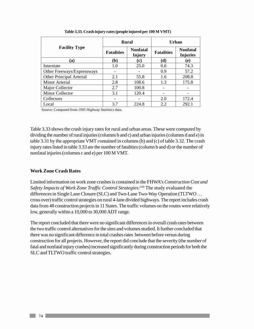
74

Table 3.33. Crash injury rates (people injured per 100 M VMT)

Source: Computed from 1995 Highway Statistics data.

Rural UrbanFacility Type

Fatalities NonfatalInjury Fatalities Nonfatal

Injuries(a) (b) (c) (d) (e)

Interstate 1.0 25.0 0.6 74.3Other Freeways/Expressways - - 0.9 57.2Other Principal Arterial 2.1 55.8 1.6 208.8Minor Arterial 2.8 108.6 1.3 175.8Major Collector 2.7 100.8 - -Minor Collector 3.1 120.4 - -Collectors - - 2.0 172.4Local 3.7 224.8 2.2 292.1

Table 3.33 shows the crash injury rates for rural and urban areas. These were computed bydividing the number of rural injuries (columns b and c) and urban injuries (columns d and e) intable 3.31 by the appropriate VMT contained in columns (b) and (c) of table 3.32. The crashinjury rates listed in table 3.33 are the number of fatalities (column b and d) or the number ofnonfatal injuries (columns c and e) per 100 M VMT.

Work Zone Crash Rates

Limited information on work zone crashes is contained in the FHWA’s Construction Cost andSafety Impacts of Work Zone Traffic Control Strategies.(18) The study evaluated thedifferences in Single Lane Closure (SLC) and Two-Lane Two-Way Operation (TLTWO …cross over) traffic control strategies on rural 4-lane divided highways. The report includes crashdata from 48 construction projects in 11 States. The traffic volumes on the routes were relativelylow, generally within a 10,000 to 30,000 ADT range.

The report concluded that there were no significant differences in overall crash rates betweenthe two traffic control alternatives for the sites and volumes studied. It further concluded thatthere was no significant difference in total crashes rates between before versus duringconstruction for all projects. However, the report did conclude that the severity (the number offatal and nonfatal injury crashes) increased significantly during construction periods for both theSLC and TLTWO traffic control strategies.

75

The 1996 Fatality Analysis Reporting System (FARS) data supports this finding. Column (a)of table 3.34 lists ranges of the percent of total motor vehicle crash fatalities that occur in workzones, while column (b) lists the number of States that fall within a range.(19)

Table 3.34. 1996 work zone motor vehicle crash fatalities as a percent of all fatalities.

Work Zone FatalityRatio Ranges (%) No. of States

(a) (b) (c)0% 3 3

0.01% – 0.49% 10.50% – 0.99% 8

9

1.00% – 1.49% 161.50% – 1.99% 7

23

2.00% – 2.49% 62.50% - 2.99% 5

11

3.00% - 3.49% 13.50% - 3.99% 1

2

4.00% - 4.49% 3 3

Inspection reveals that most SHAs are experiencing a disproportionate percentage of fatalities(more that 1 percent) occurring in work zones relative to the VMT that takes place in workzones.

Construction Cost and Safety Impacts of Work Zone Traffic Control Strategies alsoincludes crash rates on the study routes before and during the time that work zones wereestablished. The crash rates provided in the report are broken out by type of work zone, type ofconstruction work, and type of traffic control used. However, because of the limited number ofprojects in the study, the statistical validity of such highly disaggregated analysis is questionable.

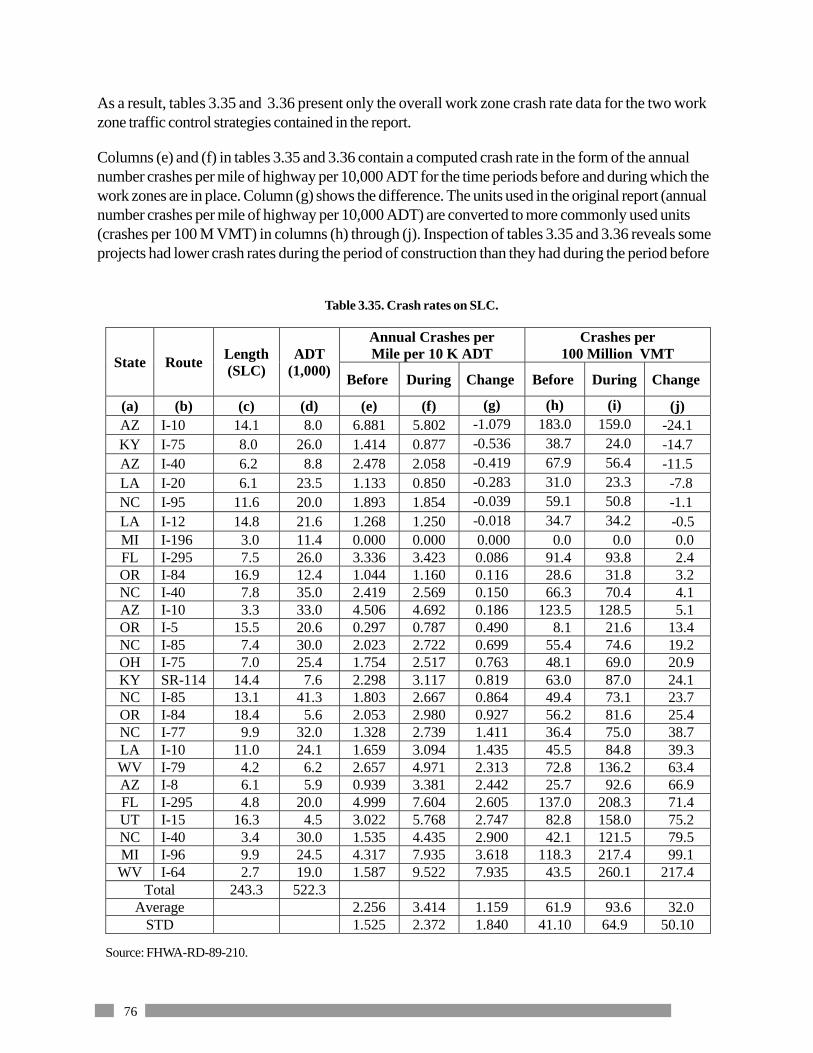
76

Source: FHWA-RD-89-210.

Table 3.35. Crash rates on SLC.

Annual Crashes perMile per 10 K ADT

Crashes per100 Million VMT

State Route Length(SLC)

ADT(1,000)

Before During Change Before During Change

(a) (b) (c) (d) (e) (f) (g) (h) (i) (j)AZ I-10 14.1 8.0 6.881 5.802 -1.079 183.0 159.0 -24.1KY I-75 8.0 26.0 1.414 0.877 -0.536 38.7 24.0 -14.7AZ I-40 6.2 8.8 2.478 2.058 -0.419 67.9 56.4 -11.5LA I-20 6.1 23.5 1.133 0.850 -0.283 31.0 23.3 -7.8NC I-95 11.6 20.0 1.893 1.854 -0.039 59.1 50.8 -1.1LA I-12 14.8 21.6 1.268 1.250 -0.018 34.7 34.2 -0.5MI I-196 3.0 11.4 0.000 0.000 0.000 0.0 0.0 0.0FL I-295 7.5 26.0 3.336 3.423 0.086 91.4 93.8 2.4OR I-84 16.9 12.4 1.044 1.160 0.116 28.6 31.8 3.2NC I-40 7.8 35.0 2.419 2.569 0.150 66.3 70.4 4.1AZ I-10 3.3 33.0 4.506 4.692 0.186 123.5 128.5 5.1OR I-5 15.5 20.6 0.297 0.787 0.490 8.1 21.6 13.4NC I-85 7.4 30.0 2.023 2.722 0.699 55.4 74.6 19.2OH I-75 7.0 25.4 1.754 2.517 0.763 48.1 69.0 20.9KY SR-114 14.4 7.6 2.298 3.117 0.819 63.0 87.0 24.1NC I-85 13.1 41.3 1.803 2.667 0.864 49.4 73.1 23.7OR I-84 18.4 5.6 2.053 2.980 0.927 56.2 81.6 25.4NC I-77 9.9 32.0 1.328 2.739 1.411 36.4 75.0 38.7LA I-10 11.0 24.1 1.659 3.094 1.435 45.5 84.8 39.3WV I-79 4.2 6.2 2.657 4.971 2.313 72.8 136.2 63.4AZ I-8 6.1 5.9 0.939 3.381 2.442 25.7 92.6 66.9FL I-295 4.8 20.0 4.999 7.604 2.605 137.0 208.3 71.4UT I-15 16.3 4.5 3.022 5.768 2.747 82.8 158.0 75.2NC I-40 3.4 30.0 1.535 4.435 2.900 42.1 121.5 79.5MI I-96 9.9 24.5 4.317 7.935 3.618 118.3 217.4 99.1WV I-64 2.7 19.0 1.587 9.522 7.935 43.5 260.1 217.4

Total 243.3 522.3Average 2.256 3.414 1.159 61.9 93.6 32.0

STD 1.525 2.372 1.840 41.10 64.9 50.10

As a result, tables 3.35 and 3.36 present only the overall work zone crash rate data for the two workzone traffic control strategies contained in the report.

Columns (e) and (f) in tables 3.35 and 3.36 contain a computed crash rate in the form of the annualnumber crashes per mile of highway per 10,000 ADT for the time periods before and during which thework zones are in place. Column (g) shows the difference. The units used in the original report (annualnumber crashes per mile of highway per 10,000 ADT) are converted to more commonly used units(crashes per 100 M VMT) in columns (h) through (j). Inspection of tables 3.35 and 3.36 reveals someprojects had lower crash rates during the period of construction than they had during the period before

77

Table 3.36. Crash rates on TLTWO.

Source: FHWA-RD-89-210.

Annual Crashes per Mile per 10 K ADT

Crashes per 100 Million VMT

State Route Length(SLC)

ADT(1,000)

Before During Change Before During Change

(a) (b) (c) (d) (e) (f) (g) (h) (i) (j)LA I-20 7.2 23.9 6.607 2.332 -4.285 181.1 61.2 -119.8UT I-15 8.8 5.2 5.447 2.815 -2.631 149.2 77.1 -72.1WV I-64 2.1 27.0 5.495 2.931 -2.565 150.5 80.3 -70.2LA US-190 2.4 16.0 9.505 7.097 -2.408 260.4 194.4 -66.0MI I-96 12.0 12.8 5.104 3.062 -2.042 139.8 83.9 -55.9FL SR-95 2.8 4.9 5.173 4.803 -0.369 141.7 131.6 -10.1MI I-94 10.0 29.0 2.884 2.535 -0.350 79.0 69.5 -9.6KY WKP 5.5 4.2 2.048 1.756 -0.293 56.1 48.1 -8.0UT I-84 10.7 3.8 3.265 3.019 -0.246 89.5 82.7 -6.7AZ I-10 2.2 12.0 2.496 2.304 -0.192 68.4 63.1 -5.3LA I-20 8.8 13.5 1.703 1.606 -0.097 46.7 44.0 -2.7OR I-5 13.2 22.6 0.978 1.043 0.065 26.8 28.6 1.8LA I-20 4.7 27.6 1.590 1.877 0.287 43.6 51.4 7.9MI I-94 10.0 18.5 3.886 4.185 0.299 106.5 114.7 8.2LA I-59 6.6 13.0 3.314 3.615 0.301 90.8 99.0 8.2NC I-40 16.9 25.0 0.980 1.700 0.720 26.8 46.6 19.7KY I-75 4.0 23.0 1.469 2.498 1.029 40.2 68.4 28.2OR I-5 7.1 24.2 0.712 1.780 1.068 19.5 48.8 29.3NC I-40 11.7 17.0 2.050 3.415 1.365 56.2 93.6 37.4WV I-77 2.6 9.3 2.516 4.193 1.677 68.9 114.9 45.9NC US-1 1.8 15.0 2.674 4.457 1.783 73.3 122.1 48.8MI I-69 6.1 15.5 1.397 4.239 2.841 38.3 116.1 77.9

Total 157.1 363.0Average 3.241 3.057 -0.184 88.8 83.6 -5.1

STD 2.191 1.384 1.697 60.0 38.0 46.8

the work zone was established. Further, from the bottom lines of the tables, the overall averagecrash rate on SLC was slightly (though not significantly) higher during work zone operations,while the overall average crash rate on TLTWO was slightly (though again not significantly)lower during work zone operations.

78

Source: FHWA/JHRP-95/1

Crash Rates per 10 M VMTWork Zone Type

Lanes inEach

Direction

Mean andStandardDeviation

WithoutWork Zone

WithWork Zone Change

Mean 6.0329 8.0431 2.0102Cross Over 2

Standard Deviation 1.6842 3.6017 3.2005Mean 5.5916 7.4528 1.8612

Partial Lane Closure 2Standard Deviation 1.4645 3.1398 3.3354

Mean 5.8278 9.3544 3.5266Cross Over 3

Standard Deviation 1.2350 5.9645 5.6871Mean 7.5166 10.1006 2.5840

Partial Lane Closure 3Standard Deviation 1.6422 2.6940 3.4964

Table 3.37. Average overall crash rates.

Source: FHWA/JHRP-95/1

Table 3.38. Average fatal and nonfatal injury crash rates.

Injury Crash Rates per 10 M VMTWork Zone Type

Lanes inEach

Direction

Mean andStandardDeviation

WithoutWork Zone

WithWork Zone Change

Mean 1.1289 2.0746 0.9457Cross Over 2

Standard Deviation 0.5376 1.9380 2.1879Mean 1.0969 2.0311 0.9342

Partial Lane Closure 2Standard Deviation 0.4252 1.3405 1.2684

Mean 1.5885 2.6367 1.0482Cross Over 3

Standard Deviation 0.3961 1.5320 1.3851Mean 1.7641 2.1128 0.3487

Partial Lane Closure 3Standard Deviation 0.2829 1.0574 1.1565

Work zone crash rate data is also included in An Evaluation of Lane Closure Strategies forInterstate Work Zone.(20) Data contained in this report was based on the study of 26 Interstate4R Projects in Indiana. Tables 3.37 and 3.38 provide data on overall and injury crash rates.

Note that the rates in tables 3.37 and 3.38 are per 10 M VMT.

Example Crash Cost Calculations

The following example problem is used to lay out a rational approach to calculating theadditional crash costs associated with a work zone-generated detour.

Problem Statement

A 5-mile rural section of Parkway between interchanges will be closed for 90 days toreconstruct a bridge taken out by flash flooding. The reconstruction will require traffic to bedetoured to a 10-mile section of rural 2-lane minor arterial highway. Capacity on the minor

79

Crash Rate Exposure

FacilityType

Crash/100 MVMT

Vehiclesper day

No. ofDays

MilesVMT

(100 M)(d)x(e)x(f)

No. ofCrashes(c)x(g)

CrashCost Rate

CrashCosts ($)(h)x(i)

(a) (b) (c) (d) (e) (f) (g) (h) (i) (j)Fatality 2.1 10,000 90 5 0.045 0.0945 1,240,000 117,180

ParkwayInjury 55.8 10,000 90 5 0.045 2.5110 27,800 69,806

Subtotal All 186,986Fatality 2.8 10,000 90 10 0.090 0.2520 1,240,000 312,480

DetourInjury 108.6 10,000 90 10 0.090 9.7740 27,800 271,717

Subtotal All 584,197

Change 397,211

Table 3.39. Crash cost calculation matrix.

arterial is currently underutilized and congestion is not expected to be a major problem. AADTon the parkway is 10,000 vehicles per day.

Solution

Table 3.39 shows the matrix used to calculate the differential crash costs. Column (c) lists thecrash rates for the facility and crash types listed in columns (a) and (b). The rates themselves aretaken from columns (b) and (c) of table 3.33. The crash fatality rate is 2.8 fatalities per 100 MVMT on rural 2-lane minor arterial highways and 2.1 on rural parkways (other principal arterialroutes). The injury crash rates per 100 M VMT is 108.6 on rural 2-lane minor arterial highwaysand 55.8 on rural parkways (other principal arterial routes).

In addition to the higher fatality and nonfatal injury crash rates, detoured and diversionary trafficon average have a greater crash exposure because of the generally greater travel distances.Column (g) of table 3.39 lists the exposure for the two alternative routes in units of 100 MVMT. The values listed were computed by multiplying the ADT (column d) by the number ofdays (column e) by the length of each alternative route (column f) and dividing the answer by100 million.

The actual number of crashes expected (column h) are calculated by multiplying the crash ratesin column (c) by the exposure in column (g).

Finally, the crash cost listed in column (j) are computed by multiplying the expected number ofcrashes in column (h) by the crash cost rates in column (i). The crash cost rates used in column(i) were selected from the updated MicroBENCOST default crash cost rates discussed earlierin Crash Cost Rates on page 23.

Further information on work zone crash rates is available in the participant’s handbook forNational Highway Institute Course # 38003, Design and Operation of Work Zone TrafficControl.(21) Pages 2-7 discuss Before and After work zone crash rates. Results from Virginiaand Texas are included.

80

Virginia data for 1991 indicate an increase of 57 percent on multilane highways and 168 percenton 2-lane urban highways with the variation being a function of traffic, geometry, andenvironment. In Texas, 1984 to 1988 data show freeway construction crashes increased by28.7 percent on the main line and 2.4 percent on frontage roads. It also shows a 37.4 percentincrease at nighttime compared to 24.4 percent during the daytime. The data also suggest thatthe average changes in severe mainline crash rates were consistent from project to project, whileother mainline crash categories varied significantly from site to site.

LCCA Microcomputer Programs

Microcomputer software programs such as MicroBENCOST and QueWZ are available forconducting LCCA on routine pavement rehabilitation projects. The simplified proceduresoutlined in this chapter are not likely to be sufficient when attempting to analyze user cost onhighly complex urban freeways. In such cases, the analyst would do better to use the battery ofurban planning models used by the major metropolitan planning organizations (MPOs). Trafficassignment models, run on the network level can provide better estimates of traffic diversionsfrom the route in question and the effect of such diversions of traffic flow on alternate routes.These models can be run to determine the network-level changes in vehicle miles of travel(VMT) and hours of traffic delay with and without the work zone in place. When network levelchanges in VMT and Delay are known, user-cost calculations become much simpler.

81

CHAPTER 4. RISK ANALYSIS APPROACH

This chapter introduces a probabilistic-based risk analysis approach to LCCA in pavementdesign. It introduces the Monte Carlo simulation technique as the method of choice in thetreatment of uncertain LCCA variables. It explores the concept of risk and examines some of thelimitations associated with the current deterministic approach. While this chapter focuses on theuse of risk analysis in a pavement design setting, the principles and techniques put forth offerpotential in other areas where uncertainty is an important consideration in the decision-makingprocess.

DEFINING RISK

The concept of risk comes from the uncertainty associated with future events — the inability toknow what the future will bring in response to a given action today. Risk can be subjective orobjective. Subjective risk is based on personal perception — intuitively deciding how risky asituation may be. For example, many people may feel that flying is more risky than driving. Thisperception of risk may be related to the consequences of failure, as well as the ability (orinability) to control the situation. Objective risk is based on theory, experiment, or observation.Often the facts of the situation may dispute intuitive feelings. For example, in 1996 there were1,070 aviation fatalities; in the same year there were also 40,676 highway fatalities. Becauseindividuals’ perceptions of risk vary, decisions incorporating risk management concepts willdepend to a large extent on the decision maker’s tolerance for risk.

DEFINING RISK ANALYSIS

Risk analysis is concerned with three basic questions about risk: 1) What can happen? 2) Howlikely is it to happen? 3) What are the consequences of its happening? Risk analysis answersthese questions by combining probabilistic descriptions of uncertain input parameters withcomputer simulation to characterize the risk associated with future outcomes. It exposes areas ofuncertainty typically hidden in the traditional deterministic approach to LCCA, and it allows thedecision maker to weigh the probability of an outcome actually occurring.

THE NEED FOR RISK ANALYSIS

Many analytical models treat input variables as discrete fixed values, as if the values were certain.In fact, the majority of input variables are uncertain. Economic models used in a typical LCCAare no exception. In conducting LCCA, it is important to be aware of the inherent uncertaintysurrounding the variables used as inputs into the analysis. Uncertainty results from theassumptions, estimates, and projections made in conducting the analysis. Table 4.1 summarizesLCCA input variables and the general basis used to determine their values.

82

Traditionally, this uncertainty is often ignored in an LCCA. For example, the analyst may make aseries of best guesses of the values for each input variable and compute a single deterministicresult. The problem with this approach is that it often excludes information that could improvethe decision.

In some cases a limited sensitivity analysis may be conducted whereby various combinations ofinputs are selected to qualify their effect on analysis results. However, even with a sensitivityanalysis, this deterministic approach to LCCA often conceals areas of uncertainty that may becrucial to decision-making process. Often, stakeholders seize upon the uncertainty associatedwith LCCA inputs and vigorously debate the validity of the results. Traditional, deterministic-based LCCA results such as these generate endless debate over which alternative truly has thelowest life-cycle cost. This process encourages division and unproductive debate.(22)

The need to make strategic long-term investment decisions under short-term budget constraintsis forcing SHAs to consider risk as a criterion for judging a course of action. Risk analysisexposes areas of uncertainty for the decision maker. Based on this new information, the decisionmaker has the opportunity to take mitigating action to decrease exposure to risk. With theemergence of user-friendly computer software, an SHA can easily integrate quantitative riskanalysis concepts into the decision-making process

GENERAL APPROACH

Figure 4.1 illustrates the basic risk analysis approach in LCCA. It shows the NPV formulatypically used as the economic indicator in an LCCA. As shown in figure 4.1, a risk analysisapproach uses random sampling from probabilistic descriptions of uncertain input variables

Table 4.1. LCCA input variables.

LCCA Component Input Variable SourcePreliminary Engineering EstimateConstruction Management EstimateConstruction Estimate

Initial and Future Agency Costs

Maintenance AssumptionTiming of Costs Pavement Performance Projection

Current Traffic EstimateFuture Traffic ProjectionHourly Demand EstimateVehicle Distributions EstimateDollar Value of Delay Time AssumptionWork Zone Configuration AssumptionWork Zone Hours of Operation AssumptionWork Zone Duration AssumptionWork Zone Activity Years ProjectionCrash Rates Estimate

User Costs

Crash Cost Rates AssumptionNPV Discount Rate Assumption

83

(initial cost, future cost, discount rate, and year of rehabilitation) to generate a probabilisticdescription of results. By performing the Monte Carlo computer simulation, thousands, eventens of thousands of samples are randomly drawn from each input distribution to calculate aseparate what-if scenario. With the speed and memory of today’s personal computers, suchiterations can be conducted in a matter of minutes or even seconds. The results generated fromeach what-if iteration are captured for later statistical analysis.

Similar to the inputs, risk analysis results are presented in the form of a probability distributionthat describes the range of possible outcomes along with a probability weighting of occurrence.In other words, by randomly drawing samples from the model’s input distributions, the computercombines the variability inherent in the inputs and summarizes it in the form of a probabilitydistribution. With this information, the decision maker knows not only the full range of possiblevalues, but also the relative probability of any particular outcome actually occurring. This isexactly the information that the decision maker needs in order to make an educated decision.

By including all possible values for the analysis inputs in relation to their probability ofoccurrence, risk analysis elevates the LCCA debate from contesting the validity of results todeciding best public policy. Armed with this new information, risk analysis provides the decisionmaker with the opportunity to take mitigating action to decrease exposure to risk. Moreover,risk analysis provides those vested with the appropriate authority and accountability, namelyexecutives and elected officials, the opportunity to make decisions about taking risk. (23)

Although the risk analysis approach is calculation intensive and would be impractical tocomplete by hand, the approach can be easily incorporated into deterministic analysis by usinguser-friendly computer software programs. Today, software is available that includes advancedrisk analysis techniques such as Monte Carlo simulation. Risk analysis software can be stand-

Figure 4.1. Computation of NPV using probability and simulation.

NPV = Initial Cost +

1(1 + i)nFuture Cost x

Combine Variability of Inputs to Generate aProbability Distribution of Results

84

alone programs (Microsoft Visual Basic, C++, etc.) or simple add-ins to spreadsheets such asMicrosoft Excel or Lotus.

Because of the flexibility that spreadsheets offer in solving a wide variety of problems thisInterim Technical Bulletin explores the use of risk analysis in a spreadsheet environment.The two most often used spreadsheet add-in risk analysis software programs are @RISK andCrystal Ball.They are very similar in operation and capability. For presentation purpose, thisTechnical Bulletin discussion uses @RISK in conjunction with Microsoft Excel spreadsheets.

Risk analysis has been used for a number of years in other industries. As a result, a number ofapproaches have evolved to conduct such analysis. The following sections outlines a generalapproach that may be used to conduct a risk analysis. The five proposed steps are:

1. Identify structure and logic of problem.2. Quantify uncertainty using probability.3. Perform simulation.4. Analyze and interpret results.5. Make a consensus decision.

The following sections address each of these steps in detail. The example problem presentedbelow illustrates how risk analysis may be applied in a pavement design LCCA setting. To keepthe example simple, user costs are omitted.

A State highway agency is considering two competing pavement designalternatives, A and B. The analysis period is 35 years, routine reactive maintenancecosts differences between alternatives are insignificant, and the discount rate mayrange from 3 to 5 percent. Average and Standard Deviations for Agency Costs,shown in table 4.2, have been developed from an analysis of recent bid records.However, because of a lack of documented field performance data, the Stateconvened a special panel of pavement experts to develop estimates of pavementservice life for each the proposed design alternatives. Table 4.3 shows theseestimates. Use a probabilistic approach to evaluate the two alternatives.

Table 4.2. Average and standard deviations for agency costs.

Alternative A Alternative BCost Item

Average Std Dev Average Std DevInitial Agency Cost

($ Millions)26.5 0.75 20.0 2.5

Future RehabilitationCost ($ Millions)

7.0 0.5 6.0 1.0

85

Step 1. Identify the Structure and Layout of the Problem

The first step in conducting a risk analysis is to identify the structure and layout of the problem.This usually involves reducing the problem to its most basic elements and describing it in theform of an analytical model. Flow charts sometimes supplement the model and clarifyrelationships between variables. In this example problem, the model is defined by the formula forNPV:

This model may be programmed in a spreadsheet or a stand-alone program may be developedusing Visual Basic, C++, etc.

Figure 4.2 shows the pavement service life curves for each alternative strategy based on themean service life values from table 4.3. Based on the mean pavement service life, Alternative A

++= ∑

)1(

1

isFutureCosttInitialCosNPV n

Figure 4.2. Pavement life curves for Alternatives A and B.

Terminal Serviceability

Pav

emen

t C

on

dit

ion

Pavement Life (Years)

RSL

0 5 10 15 20 25 30 35

Alt AAlt B

35-Year Analysis Period

Table 4.3. Estimates of pavement service life.

Alternative A Alternative B

MinMost

Likely Max MinMost

Likely MaxInitial PavementDesign (Years)

20 25 30 12 15 18

Future RehabilitationDesign (Years)

10 13 15 5 7 10

86

requires one rehabilitation; whereas, Alternative B requires three rehabilitations over the analysisperiod of 35 years. Figure 4.3 shows the expenditure streams for each alternative based on themean service life values from table 4.3.

Figure 4.3. Cash flow diagram for Alternatives A and B.

Co

st (

$ M

illio

ns)

Pavement Life (Years)

$26.5

$20.0

$6 $6 $6$7

Alt AAlt B

$1.6

$1.5

35-Year Analysis Period

0 5 10 15 20 25 3035

Based on the mean values of estimated service lives, both Alternatives A and B have remainingservice life (RSL) at the end of the 35-year analysis period. The value of the RSL must beproperly accounted for and appropriately discounted. In a deterministic LCCA, treatment of theRSL of each alternative would be relatively straightforward. In the probabilistic risk analysisapproach, the RSL issue becomes more complex because of the range of possible input valuesand the random sampling of model inputs.

The NPV model must take into account the entire range of probable pavement service lives forboth the initial design and future rehabilitation designs. As such, there is a discrete probabilitythat the last rehabilitations (as defined using mean service life values) shown in figure 4.2 couldtake place earlier than the mean service life values would indicate. At the same time there is adiscrete probability that the last rehabilitations shown might well only be required at some pointbeyond the end of the analysis period. As a result, probabilistic-based risk analysis models mustaccount for all the possibilities in determining the number, timing, and RSL of future rehabilitationrequirements. Typically, logic IF statements provided in most spreadsheet programs orprogramming languages can be used to facilitate discounting future costs over the entire range ofprobable service life values.

In developing the structure and layout of the model, it is crucial to identify dependencies amonguncertain variables to avoid producing incorrect results. Because user costs have been omittedin the example problem, the number of variables has been significantly reduced. Initial cost,future costs, discount rate, and year of rehabilitation activity are the uncertain variables in thismodel. The next step is to describe their uncertainty.

87

Step 2. Quantify Uncertainty Using Probability

The next step is to develop probability distributions for the uncertain variables identified in theprevious step. A probability distribution allows the analyst to describe the complete range ofvalues the variable may assume and weights their likelihood of occurrence accordingly.

Types of Probability Distribution

Figure 4.4 illustrates some of the more common probability distributions. Those shown includetriangle, normal, and uniform distributions in histogram format.

Cum

ulat

ive

Pro

babi

lity

4 8 12

1.00

0.75

0.50

0.25

0.0

Project Cost, ($ Millions)

75% ProbabilityProject Cost willbe Less than$9 Million

Figure 4. 5. Ascending cumulative probability distribution.

Triangle Normal Uniform

5 6 10 10 15 20 7 23

0.10

0.05

0.00

0.20

0.10

0.00

0.06

0.00

Triang(min, most likely, max) Normal(avg, std) Uniform(min, max )

Figure 4. 4. Example probability distributions.

The horizontal axis provides a range of possible values and the vertical axis provides a relativefrequency weighting of the occurrence of any particular value. For the histograms shown, theprobability is equal to the area under the curve and the total shaded area is equal to 1.0.

Figure 4.5 shows a cumulative ascending probability distribution. In this case the cumulativeprobability is read directly off the vertical axis. For the example shown, there is a 75 percentprobability that project costs will be less than or equal to $9 million. Sometimes, the cumulativedistribution is shown in the descending format, in which case the probability represents theprobability of exceeding any particular value.

88

Discrete and Continuous Variables

Probability distributions may be used to model discrete or continuous variables. Discretevariables are countable. Continuous variables are not. For example, time passes gradually;whereas the numbers on a digital wristwatch change abruptly. In this case, time is a continuousvariable, whereas, the watch’s measurement of time is not. In practice, a continuous distributionmay be used to model a discrete variable, as long as the difference between allowable values issmall. For example, project costs is a discrete variable with steps of 1 cent. However, it may bemodeled using a continuous distribution because the magnitude of agency cost are relativelylarge in a typical pavement design LCCA.

Developing Probability Distributions

Probability distributions may be developed using either objective or subjective methods. Theobjective method uses hard data (such as bid price list and observed capacity) to formulate thedistribution; the subjective method uses expert opinion.

When existing data is available, statistical analysis packages can be used to automatically fit theprobability distribution to the data. These programs compare the more common distributiontypes with available data. Along with recommendations on the distribution types that bestdescribe the variability of the data, many distribution fitting programs provide statisticalindicators such as Chi-squared, Anderson-Darling (A-D), and Kolmogorov-Smirnoff (K-S)that describe the goodness of fit. These statistics indicate how closely the probability distributionfits the data.

Figure 4.6 illustrates the use of group interviews for developing subjective probabilitydescriptions of uncertain variables. As shown, expert panels are convened to establish theboundaries and general shape of input distributions. This process of eliciting information fromexperts is similar to the well-known Delphi method. Such meetings are structured to elicit allexpert opinion. Background information is provided to participants by using scatter plots, trendcharts, basic statistics, and histograms to summarize available data. Discussion topics includenot only the over all uncertainty of the input variables, but also the possible interrelationships and

Performance Life, (years)

Rel

ativ

e F

requ

ency

8 10 12 14

Thin Overlay

Figure 4. 6. Using expert opinion to develop probability distributions.

89

codependencies among the input variables. Follow-up activities may include individualinterviews with meeting participants to ensure all opinions are included. Formal surveys andquestionnaires may also be used in the process to ensure that the resulting distribution covers theentire range of possible values. To facilitate buy-in on model results, it is important to emphasizeinvolving all stakeholders in this process.

The six distributions most often used to model the opinion of experts include:

• Triang — No tail values.• Trigen — Allow for tail values.• Normal — If the analyst believes the data to be normally distributed, a technique

is to back into the distribution, given the mean, min, and max values.The Empirical rule indicates that plus or minus 2 standard deviationsapproximate 95 percent of the data. The equation to estimate thestandard deviation is: (Max – Min)/4.

• General — This distribution is very flexible because it allows the expert task groupto tailor the shape of the curve.

• Uniform — A gross estimating tool. A problem with the uniform distribution is thatoutside the min and max values, the probability precipitously drops to 0.

• Discrete — To model known probabilities or to weight expert opinions.

Selecting Distributions and Defining Parameters

Returning to the example problem, the normal distribution will be used to model the variabilityfor agency costs using the average and standard deviations provided in table 4.2. When usinghard data to determine the type of distribution to use, it is important to check the reasonablenessof the goodness of fit statistics associated with the selected distribution. When measured datais not available, a triangular distribution may be used as a rough estimate of the distribution’sshape. For the example problem, a triangular distribution will be assumed and the data onminimum, most likely, and maximum service life data in table 4.3 will be used for the distributioninput parameters.

If nothing were known about the shape of a distribution, it might be more appropriate to use theuniform distribution and thereby give equal weight to probability of all input values. Little isknown about the variability of the discount rate in the example problem other than it ranges from3 to 5 percent. However, recalling the OMB discount rates shown in table 1.1, a symmetricaltriangular distribution with a minimum, most likely, and maximum of 3, 4, and 5 percent will beused to estimate the actual distribution. The symmetry of the triangular distribution has the addedadvantage of not giving advantage to a particular alternative based on the influence of higher or

90

lower discount rates. Typically, lower discount rates favor higher initial costs and lower futurecosts. Higher discount rates typically favor lower initial costs and higher future costs. Table 4.4summarizes the input distributions that will be used in the analysis.

Table 4. 4. Summary of input distributions for LCCA.

VariableDistribution

Type

Distribution Type and

Controlling Parameters Illustration

Initial Agency

CostNormal

Normal(mean, std dev)

Alt A – Normal(26.5, 0.75)

Alt B – Normal(20,2.5)

Rel

ativ

eP

roba

bilit

y mean

std dev

Future Rehab

CostNormal

Normal(mean, std dev)

Alt A – Normal(7, 0.5)

Alt B – Normal(6,1)

Rel

ativ

eP

roba

bilit

y mean

std dev

Pavement

Service Life –

Initial Constr.

Triangular

Triang(min, most likely, max)

Alt A – Triang(20,25,30)

Alt B – Triang(12,15,18)min max

most likely

Rel

ativ

eP

roba

bilit

y

Pavement

Service Life –

RehabilitationTriangular

Triang(min, most likely, max)

Alt A – Triang(10,13,15)

Alt B – Triang(5,7,10)min max

most likely

Rel

ativ

eP

roba

bilit

y

Discount Rate Triangular

Triang(min, most likely, max)

Alt A – Triang(3,4,5)

Alt B – Triang(3,4,5)min max

most likely

Rel

ativ

eP

roba

bilit

y

91

Incorporating Probability Distributions in Spreadsheet Models

Probability distributions can be directly incorporated into spreadsheet models using customdistribution functions available as part of the @RISK and Crystal Ball software programs. Eachof the programs includes approximately 30 additional spreadsheet functions that are add-ins tothe existing spreadsheet’s standard function set. Each of these additional functions represents aprobability distribution (NORMAL, BETA, TRIANG, etc.).

Figure 4. 7 shows a Microsoft Excel/@RISK spreadsheet model of the example problem. Itillustrates how the initial agency cost for Alternative B, shown in cell D36, can be programmedas an @RISK distribution function. Similar to a standard Excel function, an @RISK function isentered into the cell by including both the function name and argument list. Figure 4.7 showsinitial agency cost represented as a normal distribution with a mean of $20 million and astandard deviation of $2.5 million.

@RISK “add-in” buttons

Normal(20,2.5)

std dev

Figure 4. 7. Excel spreadsheet showing @RISK add-in buttons.

92

Distribution functions such as this may be used anywhere in the spreadsheet where there isuncertainty about the value of the variable. @RISK functions may be used the same way thatany of the other normal spreadsheet functions are used. They may be included in mathematicalexpressions having cell references or be used as part of IF–THEN expressions, clarifyinglogical relationships.

Step 3. Perform Simulation

After the structure of the model has been established and distributions developed andsubstituted for the uncertain input variables, the next step is to run a simulation of the model toobtain results. A simulation is essentially a rigorous extension of a sensitivity analysis that usesdifferent randomly selected sets of values from the input probability distributions to calculateseparate discrete results. The results are arrayed in the form of a distribution covering allpossible outcomes. This process of using random numbers to sample from probabilitydistributions is known as Monte Carlo sampling.(24) Figure 4.8 depicts the process of samplingfrom an input distribution.

Figure 4.8. Monte Carlo sampling showing four iterations.

0.0

0.2

0.4

0.6

0.8

1.0

Cu

mu

lativ

e P

rob

ab

ility

Random Number

.41

.57

.48

Values Sampled from Input Distribution

X.65

.65

As shown in figure 4.8, a series of random numbers between 0 and 1 are generated by thecomputer along the cumulative probability scale of the input distribution. Values correspondingto each random number are sampled along the x-scale. For the example shown, when thecomputer generates the random number 0.65 in figure 4.8, a corresponding value of x

.65 is

sampled. The sampled value is then combined with other distribution samples to compute asingle result. It is important to note that the computer uses a uniform distribution to generate therandom numbers and all values along the cumulative scale of the y-axis have equal probability ofbeing selected. Therefore, x-axis values corresponding to portions of the distribution curvewhere the slope is steeper (more vertical) have a greater likelihood of being sampled comparedto x-axis values that correspond to portions of the curve with flatter slopes.

93

In a simulation, each iteration represents a possible scenario or outcome. The results of eachiteration are captured, compiled, and subjected to rigorous statistical analysis. This process ofsampling from a probability distribution is repeated until the specified number of iterations arecompleted or until the simulation process converges (i.e., the point at which additional iterationsdo not significantly change the output distribution).

Simulation techniques, such as the Monte Carlo, typically require a large number of iterations toensure sufficient opportunity to sample low probability values. This is especially true when highlyskewed distributions are used to describe the input variables. When the number of iterationsperformed is low, clustering can occur. In this situation, sampled values are tightly clusteredaround high probability outcomes and the low probability outcomes may not be adequatelysampled. Clustering is particularly important when low probability outcomes can have aninordinately serious effect on results. Such outcomes must be accounted for in the simulation,but, to do this, they must be sampled. This has led to the development of a sampling techniqueknown as Latin Hypercube, which forces a more representative sampling with a much lowernumber of iterations. (25,26,27)

Latin Hypercube is a stratified sampling technique where the probability scale of the cumulativedistribution curve is divided into an equal number of probability ranges. The number of rangesused is equal to the number of iterations performed in the simulation.

Figure 4.9 illustrates Latin Hypercube sampling, in this case, showing four iterations, andtherefore four distinct divisions of the cumulative probability scale. As shown in figure 4.9, withina division (in this case, division number 2), a random number between 0 and 1 is generated andserves as the basis for selecting the input value. In the case shown, 0.4 is generated and a

0.0

0.2

0.4

0.6

0.8

1.0

Values Sampled from Input Distribution

Cum

ulat

ive

Pro

babi

lity

Random Number Between 0 and 1

0

1

1

2

4

3

.40

X.40

Random Number

Figure 4.9. Latin Hypercube sampling showing four iterations.

94

corresponding value is sampled from the distribution. In future iterations, the previously sampledsection is not sampled again. Because the Latin Hypercube sampling technique memorizes thesections it sampled, it therefore achieves convergence much more quickly when compared tothe Monte Carlo. In addition to being more efficient, this technique ensures low probabilityvalues are sampled and included in the simulation.

Figures 4.10 and 4.11 compare the effect of Monte Carlo and Latin Hypercube sampling whenthe number of iterations is limited to 100. As shown, 100 samples were randomly drawn fromthe normal distribution function for Initial Agency Cost Alternative B — Normal(20, 2.5).Figure 4.11 shows that the stratified Latin Hypercube sampling technique achieves a distribution

Normal(20,2.5)

Monte Carlo Sampling

0

0.020.04

0.06

0.08

0.10.12

0.14

16.4

17.4

18.4

19.4

20.4

21.4

22.4

23.4

24.4

25.4

Project Cost ($ Millions)

Rel

ativ

e P

rob

abili

ty

Figure 4.10. Monte Carlo sampling – 100 iterations.

Figure 4.11. Latin Hypercube sampling – 100 iterations.

Normal(20,2.5)

0

0.02

0.04

0.06

0.08

0.1

0.12

0.14

12.7 14.0 15.4 16.8 18.2 19.5 20.9 22.3 23.6 25.0

Project Cost ($ Millions)

Rel

ativ

e P

rob

abili

ty Latin Hypercube Sampling

95

that more resembles the familiar bell-shaped normal curve when compared to pure randomMonte Carlo sampling. Because of stratified sampling, it is possible to achieve convergence infewer iterations as compared to the Monte Carlo simulation.

A cardinal rule of risk analysis modeling is every iteration of a risk analysis simulation mustbe a scenario that can actually occur. Failure to recognize the dependent relationshipbetween input variables is usually a prime source of error in simulation modeling. Suppose, forexample, that as part of a risk model, probability distributions describe both the randomvariability for AADT and pavement service life. Typically, pavement engineers have relatedshorter pavement life to higher traffic volumes. Therefore, it would be irrational for a simulationmodel to sample the high side of the traffic probability distribution curve, and at the same time,sample the high side for pavement life. Formal treatment of this relationship between AADT andpavement service life is usually accounted for in the simulation by using a correlation matrix.Given that user costs are omitted from the example problem, the number of variables has beengreatly reduced and the analyst does not have to correlate variables. Another source of error issampling input distributions outside reasonable bounds. For example, sampling from a normaldistribution for project cost may produce misleading results, particularly when the valuessampled are negative. The use of logical statements as well as establishing bounds for thedistribution may be used to overcome errors such as this.

Figure 4.7, previously shown, is a spreadsheet that shows the results of 10,000 iterationsprocessed using a Microsoft Excel @RISK model.(28) The simulation run time was 47 secondsusing a Pentium 166 MHz Computer with 80 MB RAM. Before analyzing the simulation results,it is important to test the assumptions to make certain the model is robust across the entire rangeof possible values for the uncertain inputs. The model should be tested as each component isadded to make certain the results are reasonable. This is especially true for large and complexmodels. A visual tool to examine a model during a simulation is to construct a plot of theperformance curves and cash flows. @RISK will allow a simulation to be executed one step ata time. By stepping through the simulation and viewing the changing shape of the output graphsin real time, it is possible to detect errors that may exist in the model.

Another tool that may be used to test a risk model is to incorporate the use of a random numbergenerator seed. A seed value is a value that is used to start the sampling process and allsubsequent random numbers will rely on this value. Providing that the model is not changed, asecond run of the simulation using the same seed value will produce exactly the same results.This can be very useful in testing the effect of varying distributions on risk results. By using aseed value, the analyst can be certain that any change in the result is caused by changes in themodel and is not a result of randomness of the sampling. After the model is tested and asimulation is performed, the next step is to analyze and interpret the results.

96

Step 4. Analyze and Interpret Results

If the analysis had been conducted according to the traditional deterministic approach, all thatwould be available to base the decision on would be the means of the output distributions:Alternative A $28.79 million and Alternative B $27.32 million, respectively. Based on the NPVmeans, it is readily apparent that Alternative B is less than Alternative A by $1.47 million(~ 4.8 percent). Some SHAs would probably consider this difference in means insignificant andmay exclude lowest NPV as a consideration for selecting the alternative. Without an analysis ofthe variability about the mean, a decision such as this may prove to be a poor choice —depending on the decision maker’s tolerance for risk.

Interpretation of risk analysis results goes beyond a simple comparison of which alternative onaverage costs less by including an analysis of the likelihood that any particular outcome willoccur. There is no presumption that any particular alternative is better. Figure 4.12 shows therisk profile of the NPV for Alternatives A and B in histogram form, where the probability is thearea under the curve. As Figure 4.12 shows, the entire range of conceivable outcomes is

Figure 4.12. Histogram NPV for Alternatives A and B.

0

0.1

0.2

0.3

0.4

0.5

0.6

18 23 28 33 38

Net Present Value ($ Millions)

Rel

ativ

e P

rob

abili

ty

Alternative A Alternative B

arrayed with the estimated probability of each outcome actually occurring. The main advantageof the histogram is that it readily shows the variability about the mean. The wider the distribution,the greater the variability. As shown, the outcome for Alternative B is more uncertain thanAlternative A.

97

Figure 4.13. Cumulative risk profile of NPV for Alternatives A and B.

0

0.2

0.4

0.6

0.8

1

18 23 28 33 38

Net Present Value ($ Millions)

Rel

ativ

e C

um

ula

tive

Pro

bab

ility

Alternative A Alternative B

60%

$28.27

In interpreting the risk profile in figure 4.12, it is important to distinguish between upside riskand downside risk. Downside risk for project cost implies cost overrun — chance of financialfailure. Upside risk for project costs implies cost underrun — opportunity for low cost. Asfigure 4.12 shows, Alternative B has greater upside risk compared to Alternative A. However,as discussed below, it is important to quantify the probability of cost overrun for Alternative B.

Figure 4.13 shows the risk profiles for Alternatives A and B in cumulative form. As shown,there is a 60 percent probability that project costs for Alternative B will be less than

$28.27 million. This means that for the 10,000 iterations that were processed, 60 percent of thecalculated values for NPV were less than $28.27 million. The variability for the proposedalternative is inversely proportional to the slope of the cumulative curve. In other words, thesteeper the slope, the less variability. The flatter the slope, the greater the variability. As shown,the slope for Alternative B is flatter than that for Alternative A, and is therefore more variable.

A risk analysis provides much more information than a simple deterministic solution. As table4.5 shows, additional information comes in the form of basic statistical measures of simulationresults that reveals the underlying uncertainty associated with each alternative. In interpreting therisk involved with each alternative, it is important to identify the magnitude of the extremes of thedistributions shown in figure 4.12. As table 4.5 shows, Alternatives A and B have minimums of$25.4 and $13.3 million and maximums of $33.04 and $40.35 million, respectively. Thestandard deviation for Alternative B is much greater than Alternative A. Analysis of thedistribution tails reveals a 10 percent probability that the NPV of Alternative B will be less than

98

Net Present Value ($ Millions)Basic Statistic Alternative A Alternative B B – A

Minimum $ 25.40 $ 13.13 $ (12.27)Maximum 33.04 40.35 7.31

Mean 28.93 27.60 (1.33)Std Deviation 1.04 3.13 2.09

Percentile5% 27.33 22.66 (4.67)

10% 27.65 23.71 (3.94)15% 27.88 24.39 (3.49)20% 28.05 24.98 (3.07)25% 28.22 25.50 (2.72)30% 28.36 25.93 (2.43)35% 28.49 26.34 (2.15)40% 28.62 26.73 (1.89)45% 28.75 27.12 (1.62)50% 28.87 27.48 (1.40)55% 29.00 27.87 (1.13)60% 29.13 28.27 (0.86)65% 29.27 28.71 (0.56)70% 29.42 29.13 (0.29)75% 29.58 29.63 0.0680% 29.76 30.20 0.4485% 30.01 30.88 0.8790% 30.31 31.67 1.3595% 30.75 32.98 2.23

Table 4.5. Risk profile statistics for Alternatives A and B.

Alternative A by as much as $3.94 million. Conversely, there is a 10 percent probability thatAlternative B will exceed the cost of Alternative A by $1.35 million. However, 70 percent of thetime, the NPV for Alternative B was less than Alternative A. It is interesting to point out that themean shown in table 4.5 for Alternatives A and B is slightly different from the expected valuesshown in figure 4.7. This is because table 4.5 means are based on a simulation of 10,000iterations.

As part of the risk assessment, a sensitivity analysis can be performed on simulation results toidentify significant input variables that are important in determining the output distributions. Theresults of this analysis are usually displayed in the form of a Tornado plot, as shown in figures4.14 and 4.15. The higher the correlation coefficient, the more significant the input variable is ondetermining the results. The variables listed at the top of the graph are more significant thanthose at the bottom. The degree of correlation may be calculated using either the rank ordercorrelation or stepwise least squares regression. Rank order correlation makes no presumption

99

-1.00 -0.50 0.00 0.50 1.00

Correlation Coefficient

Design Period / Life Rehabs

Agency Cost Rehabs

Discount Rate

Initial Agency Cost

Design Period / Life Initial Construction

-0.4 -0.2 0 0.2 0.4 0.6 0.8 1

Design Period / Life Initial Construction

Design Period / Life Rehabs

Initial Agency Cost

Agency Cost Rehabs

Discount Rate

Correlation Coefficient

Figure 4.14. Correlation sensitivity plot for NPV Alternative A.

Figure 4.15. Correlation sensitivity plot for NPV Alternative B.

about the relationship between the input and output variables. Least squares regression assumesa linear relationship between input and output variables. This is important to note becausemodels that incorporate divisions and power functions often violate this later assumption. Bothfigures 4.14 and 4.15 use rank order correlation. Typically, correlation coefficients less thanabout 0.6 are not significant.

Figure 4.14 shows Initial Agency Cost has a correlation coefficient of 0.72. This means thatif Initial Agency Cost moves one standard deviation (in either direction), then the NPV forAlternative A will move 0.72 of a standard deviation in the same direction. If Design Period/

100

0

0.2

0.4

0.6

0.8

1

18 23 28 33 38

Net Present Value ($ Millions)

Rel

ativ

e C

um

ula

tive

Pro

bab

ility

Alternative A Alternative B

Which Inputs“Drive” the Shaded

Tail of Alt-B?

Figure 4.16. Analysis of distribution tails.

Life Initial Construction moves one standard deviation (in either direction), then expectationsare that the NPV for Alternative A will move 0.52 standard deviations in the opposite direction,because the relationship is reversed as indicated by the negative correlation coefficient.

To further the evaluation, the analyst can explore the low probability area of the outcomedistribution curve for Alternative B, where the NPV is greater than that for Alternative A,(i.e., greater than the 90th percentile). Figure 4.16 illustrates the need to identify the key inputvariables that produce low probability scenarios — the extremes, or tails, of the resultsdistribution for Alternative B.

A scenario analysis can identify those variables that may cause a project to have significantcost overrun. The analysis is easily accomplished using Excel/@RISK, which uses the followingprocedure to identify significant inputs for a particular scenario.

1. Each input variable that affects the selected output is found.2. The median and standard deviation of each input is calculated.3. A subset is created containing only the iterations in which the output achieves the

defined target.4. The median of each input found in step 1 is calculated for the subset data.5. For each input found in step 1, the difference between the simulation median and the

subset median is calculated and compared to the standard deviation of the input data.If the absolute value of the difference in medians is greater than 0.5 of the standarddeviation of the whole, then the input variable is deemed significant — otherwise the

input is ignored.

101

Significant Inputs When NPV Alternative BGreater Than 90th Percentile

Median of Samples in SubsetIterations Meeting Target

Design Period/Life Initial Construction (Years) 14.1Agency Cost Initial Construction ($ Millions) 21.8Agency Cost Rehabs ($ Millions) 5.43

Table 4.6. Scenario analysis results for NPV Alternative B.

Table 4.6 identifies the significant inputs in the upper 10 percent of the distribution forAlternative B as Design Period/Life Initial Construction, Agency Cost Initial Construction,and Agency Cost Rehabilitation. Now that the drivers in the tail are known, the decisionmaker may choose to take some mitigating action against these significant inputs to reduceexposure to upside risk. For example, the decision maker may choose to aggressively controlagency costs.

Step 5. Make Consensus Decision

In order to make a decision based on risk analysis results, it is important for the decision makerto define the level of risk the organization can tolerate. Decision makers who can tolerate littlerisk prefer a small spread in possible results, with most of the probability associated withdesirable results. Conversely, if decision makers are risk-takers, then they will accept a greateramount of spread, or possible variation in the outcome distribution. Most decision makers canreach a consensus decision after weighing the probability for upside and downside risk. In ourexample, clearly Alternative B appears to be the better alternative since there is far greaterlikelihood of cost savings compared to Alternative A. Also, the probability of cost overrun,compared to Alternative A, appears to be quite low — less than 30 percent.

The reason that this step is called a consensus decision is because all stakeholders wereinvolved in developing the input probability distributions early in the process. As a result, thisoverall process should diffuse any negative reaction special interest groups may have with theoutcome. The result is that the entire risk analysis process facilitates consensus building amongstakeholders so that action, in the best public interest, may be taken.

PRESENTING RISK ANALYSIS RESULTS

A risk analysis is of little value if the results cannot be understood. Thus, this section offerspractical advice in presenting risk analysis results to decision makers. The first step in presentingrisk analysis results is to know the audience. Here are some basic questions to ask prior topresenting the results.

• Does the audience need a risk primer?• Does the audience buy in to the risk analysis approach?• Does the audience buy in to the analysis?

Does the audience need a risk primer? One of the primary reasons people have difficultyinterpreting risk analysis results is they often have little understanding of basic statistics which is a

102

prerequisite to interpreting risk results. Therefore, it may be necessary to provide anintroductory session to train decision makers on fundamental risk analysis concepts such asMonte Carlo sampling and probability distributions before presenting risk analysis results. Thepurpose of such a session is to provide just enough information so the decision maker canunderstand and interpret risk analysis results. There is no reason to include a formal treatment ofthe statistical theory underlying the concepts.

Does the audience buy in to the risk analysis approach? Although simulation techniqueshave been around since the early 1940s, it is only recently that these techniques have beenemployed in the spreadsheet world of the analyst. Risk analysis is therefore a relatively new wayof treating uncertainty and involves an entirely new approach to understand and interpret theresults. Risk analysis is an analytical tool to aid the decision maker to select the best alternative.By exposing previously hidden areas of uncertainty critical information is revealed therebyproviding the decision maker the opportunity to take mitigating action to decrease exposure torisk. Most importantly, risk analysis provides those vested with the appropriate authority, namelyexecutives and elected officials, the opportunity to make decisions about risk taking. As acompliment to LCCA, risk analysis elevates the debate—from the validity of LCCA results—to taking action that is in the best interest of the general public.

Does the audience buy-in to the analysis? Anyone examining risk analysis results should becautious. First and foremost is the model correct? There is nothing worse than making highstakes decisions based on a model that is wrong. It is important that the structure and logic ofthe model be verified by an independent party, particularly, if risk analysis becomes an integralpart of the decision making process.

Does the model follow generally accepted procedures? For example, there are a numberof different procedures available to determine user costs. Are the procedures that are employeddocumented and do stakeholders, in general, accept the procedures? This is important toobtain buy-in on risk results. How were the input distributions determined? Were stakeholdersinvolved in the process? Does the range for the distributions fall within a generally acceptedrange? Finally, the level of detail in a risk analysis report should be commensurate with theproblem at hand.

The presenter of a risk analysis report should be able to answer key questions regarding the riskanalysis results. In the presentation, it is recommended that the developer of the risk model bepresent to answer key questions about the structure and logic of the model. In presenting riskanalysis results it is important not to overburden the audience with statistics. A simple 1-pagesummary to include summary statistics, histogram and cumulative distributions, and perhaps aTornado graph to show the important inputs in the analysis should be sufficient. When conveyingprobability graphs to upper management it is highly recommended that either cumulative ascend-ing or cumulative descending graphs be presented. The presenter should choose a presentationmethod and stay with it. Structure and logic charts are also quite useful in presenting the simula-tion process as well as discussing judgements about the model relationships. Place modelassumptions at the back of the report. These are important, but not so important as to be in thesummary sheet.

103

1 Highway Infrastructure Report, Office of Inspector General, Government Accounting Office,1994.

2 Federal Register, Code of Federal Regulations, Part 627, Vol.62, No.31, February 14, 1997,p. 6866.

3 Office of Management and Budget Circular No.A-94, October 29, 1992.

4 LCC Final Policy Statement, Federal Register, Vol.61, No.182, September 18, 1996,p. 35404.

5 James W. Mack, Life Cycle Costing: A Discussion Regarding Its Use for ComparingAlternative Designs, Appendix A.

6 Pavement Rehabilitation Manual, Federal Highway Administration, Washington, DC, 1990.

7 Transfund Project Evaluation Manual, The World Bank, May 1997.

8 Bosher Al-Omai and Michael I. Darter, Relationship Between IRI and PSR, Civil Engineeringstudies No. 60, Transportation in Engineering Series, University of Illinois, Champaign-Urbana,September 1992.

9 Arnim Meyburg et al., Review and Development of Life-Cycle Cost and Network AnalysisProcedures for NYSDOT Highway Pavements, Draft, August 1997.

10 NCHRP Report 133, Procedures for Estimating Highway User Costs, Air Pollution, andNoise Effects, 1972.

11 Robly Winfrey, Economic Analysis for Highways, International Textbook Company, 1969.

12 Nationwide Personal Transportation Survey, Bureau of Transportation Statistics inCooperation with the Federal Highway Administration, 1990.

13 Design for Pavement Structures, American Association of State Highway andTransportation Officials, Washington, DC, 1993.

14 Special Report 209, Highway Capacity Manual, 3rd ed., Transportation Research Board,National Research Council, Washington DC, 1994.

15 Traffic Monitoring Guide, FHWA, 3rd ed., February 1995.

16 Highway Capacity Manual, p. 6-11.

REFERENCES

104

17 1995 Highway Statistics, Federal Highway Administration, Publication No. FHWA-PL-96-017, November 1996.

18 Construction Cost and Safety Impacts of Work Zone Traffic Control Strategies, FHWAPublication No. RD-89-210, December 1989.

19 1996 Fatality Analysis Reporting System, National Highway Traffic Safety Administration,DOT-HS-82649, December 1997.

20 An Evaluation of Lane Closure Strategies for Interstate Work Zones, Final Report forthe Joint Highway Research Project, FHWA/JHRP-95/1, November 1995.

21 Design and Operation of Work Zone Traffic Control, National Highway InstituteCourse #38003, pp 2-7.

22 David Lewis, “The Future of Forecasting—Risk Analysis as a Philosophy of TransportationPlanning, TR News 177, April 1995.

23 Ibid.

24 R.Y. Rubinstein, Simulation and the Monte Carlo Methods: John Wiley and Sons, NewYork, NY, 1981.

25 R.L. Inman, J.M. Davenport, and D.K. Zeigler, Latin Hypercube Sampling (A ProgramUsers Guide), Technical Report SAND79-1473, Sandia Laboratories, Albuquerque, NM,1980.

26 R.A. Startzman and R.A. Wattenbarger, An Improved Computation Procedure for RiskAnalysis Problems With Unusual Probability Functions: SPE Hydrocarbon Economics andEvaluation Symposium Proceedings, Dallas, TX, 1985.

27 R.L. Inman, W.J. Conover, and R.J. Beckman, A Comparison of Three Methods forSelecting Values of Input Variables in the Analysis of Output from a Computer Code,Technometrics, 1979, p. 211, 239-245.

28 David Vose, Quantitative Risk Analysis: A Guide to Monte Carlo Simulation Modelling,John Wiley & Sons, New York, July 1997.

105

PUBLICATIONSFederal Highway Administration

Construction Costs and Safety Impacts of Work Zone Traffic Control Strategies, Vol.2:Information Guide, FHWA, Publication No. FHWA-RD-89-210, December 1989.

FHWA Highway Pavements Course, Chapter 14-1, National Highway Institute CourseNo.13114, Publication No. FHWA-HI-90-028, May 1990.

James S. Gillespie, FHWA/VTRC 98-R12, Estimating Road User Costs as a Basis forIncentive/Disincentive Amounts in Highway Construction Contracts, February 1998.

LCC Interim Policy Statement, Federal Register Vol.59, No.131, July 11, 1994, p. 35404.

LCC Symposium Report No.12, Life-Cycle Cost Analysis Conference Proceedings,November 1994.

Matt Witczak, Ph.D., Probabilistic-Based MCP (Micro-Computer Program) for LCCA forAsphalt Concrete Pavements, University of Maryland at College Park, May 1994.

Motor Vehicle Accident Costs, Technical Advisory, FHWA, October 31, 1994.

Ratkim Pal and Kumares C. Sinha, An Evaluation of Lane Closure Strategies for InterstateWork Zones, Joint Highway Research Project, FHWA/INJHRP-95/1, Purdue University/Indiana Department of Transportation, November 1995.

Searching for Solutions; A Policy Discussion Series, No.16, Exploring the Application ofBenefit/Cost Methodologies to Transportation Infrastructure Decision Making, (May 1995Conference Proceedings), July 1996.

Traffic Monitoring Guide, Federal Highway Administration, Publication No. FHWA-PL-95-031, October 1996.

National Cooperative Highway Research Program (NCHRP)

Project reports are issued at the conclusion of each NCHRP research project.

Report 133 Procedures for Estimating Highway User Costs, Air Pollution, and NoiseEffects, 1972.

Synthesis publications are a series of reports of studies on current practice in the field ofhighway transportation. Projects are sponsored by AASHTO.

Synthesis Report 112: Life-Cycle Cost Analysis of Pavements, 1985.

APPENDIX: RESOURCES

106

Synthesis Reports 110 and 77 address future maintenance needs and costs.

Synthesis Report 142: Methods of Cost Effectiveness Analysis for Highway Projects,1988.

Synthesis Project 20-5, Topic 27-12 Road User and Mitigation Costs in HighwayPavement Projects, Final Draft, November 1997.

Research Projects

NCHRP-1-33 Methodology to Improve Pavement Investment Decisions

NCHRP 1-34 Guidelines for Subsurface Drainage; Final Report, February 1998.

NCHRP 12-43 Life-Cycle Cost Analysis of Bridges, 1997.

Project 2-18 FY91 Research Strategies for Improving Highway User Cost-EstimatingMethodologies; Hickling, Louis, Brod, April 1994.

Project 2-18 (2)FY93 Valuation of Travel—Time Savings and Predictability in CongestedConditions for Highway User Cost Estimation Procedure, Hickling,Louis, Brod, July 1995.

Project 2-18 (3)FY94 Development of an Innovative Highway User-Cost EstimationProcedure; Hickling, Louis, Brod, March 1995.

Project 2-18 (4)FY95 Proposal—Development and Demonstration of StratBENCOSTProcedure; Hickling, Louis, Brod, (anticipated completion, November1998).

Project 7-12 Microcomputer Evaluation for Highway User Benefits,October 1993.

Project 10-50 Strategies for Rehabilitation—Rigid Pavements Subjected to High-Traffic, Draft Interim Report (Revised), Nichols Consulting Engineers,March 1998.

AASHTO

LCCA Survey, Summer 1994.

A Manual on User Benefit Analysis of Highway and Bus Transit Improvement, 1977.

The World Bank

Anthony Boardman, Aidan Vining, and W.G. Waters II, Cost and Benefits throughBureaucratic Lens: Example of a Highway Project.

107

COMPUTER SOFTWARE

Selected Sources of Software

McTrans and PC Trans

McTrans and PC Trans are microcomputer software distribution centers for transportation-related software, including public domain software such as MicroBENCOST and QueWZ,which were developed with Federal funds. For information, contact:

McTrans PC Transphone: 352-392-0378 phone: 785-864-5658fax: 352-392-3224 fax: 785-864-3199Web site: www.mctransce.ufl.edu Web site: www.kuhuh.cc.ukans.edu./~pctrans.email:uftrc@ce.ufl.edu email: pctrans@kuhuh.cc.ukans.edu.

Other Software

There are several powerful microcomputer-based risk analysis software programs currently onthe market that work well in conjunction with Lotus and Microsoft® Excel spreadsheetapplications. Authors of this Technical Bulletin have used @Risk and Crystal Ball.

@Risk Crystal BallPalisade Corporation Decisioneering Corporationphone: 1-800-432-7475 phone: 1-800-289-2550Web site: www.palisade.com Web site: www.decisioneering.com

Other software programs may be commercially available.

For information on DataPave, contact FHWA Customer Support 423-481-2967. Web site is:http://DataPave.fhwa.dot.gov, http://www.LTPPDatabase.com/main.htm,email:LTPPinfo@fhwa.dot.gov