Life-Cycle Assessment of Urban Water Provision:Tool and Case Study in California

Jennifer Stokes1 and Arpad Horvath, M.ASCE2

Abstract: The exploration of life-cycle energy use and environmental effects from U.S. water infrastructure has been limited in spite of thestrong connection between energy and water use. This research presents a methodology for quantifying the life-cycle energy consumption andassociated air emissions from water supply, treatment, and distribution. A decision-support tool, the Water-Energy Sustainability Tool(WEST), has been developed to aid such analysis. WEST calculates the environmental effects of material production, including the supplychain, material delivery and transportation, construction and maintenance equipment use, energy production, and sludge disposal. Deter-ministic and probabilistic results for a California case study utility are provided to show the tool’s capabilities. Results indicate that producinga million liters of water consumes 5.4 GJ and produces 390 kg of CO2-equivalent greenhouse gases. Energy production is the most significantactivity (50%), but material production, especially for treatment chemicals, is also important (37%). This case study is contrasted with twopreviously published case study utilities, and the reasons for the range of results are analyzed. The results demonstrate that estimating watersupply’s energy needs and emissions without a life-cycle lens can underestimate the total effects significantly. DOI: 10.1061/(ASCE)IS.1943-555X.0000036. © 2011 American Society of Civil Engineers.

CE Database subject headings: Water supply; System analysis; Sustainable development; Water use; Renewable energy; California.

Author keywords: Water supply; Systems analysis; Sustainability; Energy.

Introduction

Water system sustainability incorporates a variety of considera-tions, including economic, engineering, social, and environmentalissues. Past studies have proposed indicators for water system sus-tainability in all categories (e.g., Lundin and Morrison 2002;Sahely et al. 2005). The traditional engineering perspective onlyevaluates economic and engineering performance to determine sys-tem sustainability, though equity and other social issues can factorinto some decisions (e.g., Calijuri et al. 2005). Environmental con-siderations are generally limited to assessing preexisting environ-mental hazards and sensitive receptors in the area (e.g., residences,endangered species, wetlands).

This study addresses other important but often neglected con-siderations of environmental sustainability. Two major componentsof achieving water system environmental sustainability are:(1) water consumption occurs at or below the rate at which freshwater is returned to the source (i.e., renewing or maintaining, ratherthan depleting, the source); and (2) the material and energy inten-sity of water infrastructure are minimized and can be continuedlong-term. The effects of overconsumption have been discussed(e.g., Calijuri et al. 2005; Hall et al. 2000) and are site-specific,depending on climate, geography, hydrology, and ecology.

Prior research has determined that energy contributes signifi-cantly to the environmental effects of water. Water and energyare interconnected. Water is used to produce energy (hydropower)and as an input to generation (e.g., cooling water). Energy is neededto provide water to customers. Some estimates put current water-related electricity use at approximately 20% of California’s totalconsumption [California Energy Commission (CEC) 2005;Navigant Consulting 2006]. This includes water used for publicwater and wastewater processing, agricultural uses, industrial waterpumping and processing, and residential/commercial/industrial enduses (e.g., water heating).

Water is necessary for life and will be provided even when thebest available alternative is costly. However, system plannersshould aspire to minimize energy and material use and associatedenvironmental effects. These effects—the second area of water’ssustainability—are more generalizable between diverse systemsthan overconsumption concerns and provide the focus forthis paper.

The environmental effects of material and energy intensity arerarely considered and can inform water utility decision makingwhen used in conjunction with conventional design criteria. Asan example, many coastal California utilities are considering con-structing desalination plants to provide a reliable and local watersource. Some are also considering adding solar power capacityto reduce the greenhouse gas (GHG) emissions. However, whileGHGs are not emitted on-site when using solar power, emissionsare created during the upstream processing of photovoltaics andother solar power equipment. Using a life-cycle assessment(LCA) framework, and specifically the tool described in this paper,a utility can utilize a more comprehensive comparison of all result-ing GHG emissions in their decision process. Many other system-wide or process-specific decisions can be evaluated with LCAusing the framework presented in this paper, including selectingpipe materials, filters (conventional versus membrane), disinfectionprocesses, or different operational strategies.

1Assistant Research Engineer, Institute of Transportation Studies, Univ.of California, Berkeley, CA 94720 (corresponding author). E-mail:jrstokes@cal.berkeley.edu

2Professor, Dept. of Civil and Environmental Engineering, Univ. ofCalifornia, Berkeley, CA 94720.

Note. This manuscript was submitted on November 20, 2009; approvedon June 22, 2010; published online on September 22, 2010. Discussionperiod open until August 1, 2011; separate discussions must be submittedfor individual papers. This paper is part of the Journal of InfrastructureSystems, Vol. 17, No. 1, March 1, 2011. ©ASCE, ISSN 1076-0342/2011/1-15–24/$25.00.

JOURNAL OF INFRASTRUCTURE SYSTEMS © ASCE / MARCH 2011 / 15

J. Infrastruct. Syst. 2011.17:15-24.

Dow

nloa

ded

from

asc

elib

rary

.org

by

KA

NSA

S ST

AT

E U

NIV

LIB

RA

RIE

S on

07/

17/1

4. C

opyr

ight

ASC

E. F

or p

erso

nal u

se o

nly;

all

righ

ts r

eser

ved.

Approach and Methods

The paper is intended: (1) to produce a model to identify and in-ventory material and energy inputs and material and environmentaloutputs associated with urban water systems; (2) to deterministi-cally and probabilistically quantify the environmental effects of ur-ban water systems; and (3) to identify uncertainties and sensitivitiesin estimating the energy use of urban water systems.

The writers have developed an analytical, computer-based de-cision-support tool, the Water-Energy Sustainability Tool (WEST)to assist water supply utilities, engineering designers, planners,policymakers, and other decision makers in assessing the environ-mental effects of their infrastructure decisions. In this paper, wedescribe the structure and calculations of WEST and demonstratethe capabilities of the tool by analyzing a California utility.

Prior publications mention the existence of WEST but do notdetail the tool’s methodology, rather provide results for othercase studies (Stokes 2004; Stokes and Horvath 2006; Stokesand Horvath 2009). This paper provides details about the life-cycleactivities analyzed in WEST, documents the equations and assump-tions used, explains revisions for energy emission factors (EFs) toinclude the life-cycle effects (i.e., material acquisition, processing,and transport), and describes the recently added sludge disposalactivity. A new case study of a large California water utility whichuses local and imported water is also presented to provide a morediverse analysis of water systems. This utility serves about six timesmore people than prior case studies and therefore provides insightinto extant economies of scale. In addition, the case study expandsthe potential range of environmental effects by focusing onimported water in California.

Life-Cycle Assessment

WEST incorporates LCA, a quantitative method for assessing thecradle-to-grave environmental effects of materials, products, proc-esses, or services. Complete descriptions of the existing process-based LCA models and economic input-output analysis-basedLCA (EIO-LCA) models are available in other publications(e.g., Carnegie Mellon University Green Design Institute 2007;Hendrickson et al. 1998, 2006). This research implements a tieredhybrid LCA methodology (Suh et al. 2004), combining elements ofprocess-based LCA and EIO-LCA as shown in Table 1.

Previous environmental LCAs of urban water systems are lim-ited. One of the two representative studies was a process-basedLCA of the Belgian water cycle (pumping station to wastewatertreatment) that determined that the effects of discharging untreatedor marginally treated wastewater are more important than opera-tional effects such as energy use (Lassaux et al. 2007). A secondstudy evaluated water and wastewater services projected for 2021in Sydney, Australia (Lundie et al. 2004) and concluded that de-mand management, energy efficiency and generation, and efficientbiosolids recovery improved all environmental indicators; othertreatment alternatives produced mixed results for the indicatorsreported. The Australian study did not evaluate the constructionprocess. Both of these studies included assessments of wastewaterprocessing, a future step in the scope of this research. Table 2 sum-marizes the findings of other key water LCAs and the distinctionsbetween those studies and the one published herein (adapted fromStokes and Horvath 2009). Only one study evaluated infrastructurein the United States (Filion et al. 2004), and none explicitly used ahybrid LCA approach.

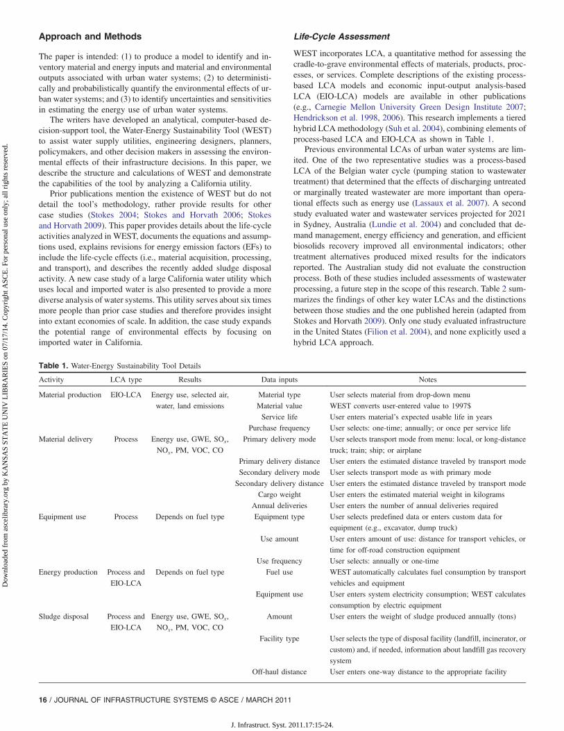
Table 1. Water-Energy Sustainability Tool Details

Activity LCA type Results Data inputs Notes

Material production EIO-LCA Energy use, selected air,

water, land emissions

Material type User selects material from drop-down menu

Material value WEST converts user-entered value to 1997$

Service life User enters material’s expected usable life in years

Purchase frequency User selects: one-time; annually; or once per service life

Material delivery Process Energy use, GWE, SOx,

NOx, PM, VOC, CO

Primary delivery mode User selects transport mode from menu: local, or long-distance

truck; train; ship; or airplane

Primary delivery distance User enters the estimated distance traveled by transport mode

Secondary delivery mode User selects transport mode as with primary mode

Secondary delivery distance User enters the estimated distance traveled by transport mode

Cargo weight User enters the estimated material weight in kilograms

Annual deliveries User enters the number of annual deliveries required

Equipment use Process Depends on fuel type Equipment type User selects predefined data or enters custom data for

equipment (e.g., excavator, dump truck)

Use amount User enters amount of use: distance for transport vehicles, or

time for off-road construction equipment

Use frequency User selects: annually or one-time

Energy production Process and

EIO-LCA

Depends on fuel type Fuel use WEST automatically calculates fuel consumption by transport

vehicles and equipment

Equipment use User enters system electricity consumption; WEST calculates

consumption by electric equipment

Sludge disposal Process and

EIO-LCA

Energy use, GWE, SOx,

NOx, PM, VOC, CO

Amount User enters the weight of sludge produced annually (tons)

Facility type User selects the type of disposal facility (landfill, incinerator, or

custom) and, if needed, information about landfill gas recovery

system

Off-haul distance User enters one-way distance to the appropriate facility

16 / JOURNAL OF INFRASTRUCTURE SYSTEMS © ASCE / MARCH 2011

J. Infrastruct. Syst. 2011.17:15-24.

Dow

nloa

ded

from

asc

elib

rary

.org

by

KA

NSA

S ST

AT

E U

NIV

LIB

RA

RIE

S on

07/

17/1

4. C

opyr

ight

ASC

E. F

or p

erso

nal u

se o

nly;

all

righ

ts r

eser

ved.

Description of the WEST Model

WEST is a scalable, MS Excel-based tool, nationally applicablein the United States, and developed based on ISO 14040 (ISO1997). This tool can assess the environmental effects of most watersources, such as imported, desalinated, recycled, surface, andgroundwater. WEST is designed so that a user without LCA exper-tise can assess the infrastructure-related environmental effects of awater system. The tool incorporates information on five activities:material production, material delivery and transportation, construc-tion and maintenance equipment use, energy production, andsludge disposal. Table 1 summarizes the input data needed andspecifies the LCAmethodology used and results calculated for eachactivity.

For each water source i, WEST calculates the total environmen-tal burden for a particular chemical or effect j (e.g., GHGemissions) according to Eq. (1)

Btotal;ij ¼ BMP;ij þBMD;ij þBEU;ij þBEP;ij þBSD;ij ð1Þ

where Btotal;ij = total burden reported in terms of mass; BMP;jj = bur-den attributable to material production; BMD;ij = burden attributableto material delivery; BEU;ij = burden attributable to equipment use;BEP;ij = burden attributable to energy production; and BSD;ij = bur-den attributable to sludge disposal. WEST calculates annual aver-age results for energy consumption and selected air, water, and landemissions. In this paper, we report air emissions including theglobal warming effect (GWE) [GHGs emitted in units of carbondioxide (CO2) equivalents] (Pacca and Horvath 2002), nitrogenoxides (NOx), sulfur oxides (SOx), particulate matter (PM), volatileorganic compounds (VOC), and carbon monoxide (CO). Resultsare normalized to a user-defined functional unit, in this case 1 mil-lion liters (ML), which represents the indoor residential demand of

approximately 4,500 people in California per year (Gleicket al. 2003).

The emissions associated with each activity are calculated assummarized in the following sections. WEST scenarios can be de-fined by the user for different water sources (e.g., imported water,desalinated water, recycled water, surface water, and groundwater),or for smaller components (e.g., treatment plant design options,such as disinfection or filtration alternatives). WEST also catego-rizes the emissions according to life-cycle phase (construction,operation, maintenance, and end-of-life) and water supply phase(supply, treatment, and distribution). The long-term effects ofsludge disposal are the only contributors to the end-of-life phasein WEST. Other end-of life-impacts of water infrastructure arenot included due to lack of data. However, given the long life-spanof most water infrastructure, effects of the end-of-life phase havebeen shown to be insignificant in prior studies (Friedrich 2002).

Material Production

The material production module uses EFs from both EIO-LCA(1997 U.S. Industry Benchmark model) and a process-based data-base,GaBi (GaBi) to estimate the environmental effects of productswhich comprise water systems. Common water system materialscan be selected from a drop-down menu by the WEST user. GaBiis used for plastic piping and certain chemicals, while all other ma-terials are associated with an economic sector based on the NorthAmerican Industry Classification System definitions as listed onthe 1997 model year EIO-LCA website (Carnegie Mellon Univer-sity Green Design Institute 2007). A representative list of materialsincludes pipes, valves, fittings, utility boxes, flowmeters, pumps,motors, electrical and control equipment, structures, chemicals,filter media, membranes, and water tanks.

Table 2. Summary of Water LCA Literature (adapted with changes from Stokes and Horvath 2009)

Reference Summary

Herz and Lipkow 2002 RESULTS: Compared dig and no-dig installation for a variety of sewer and distribution pipe materials; no-dig installation

reduced CO2 emissions by 20–30%; for water, lining pipes with mortar extended life and improved results

DISTINCTIONS: Germany focus; process-based; evaluated only distribution system

Friedrich 2002 RESULTS: Compared treatment by conventional filters and membranes; either could be preferred depending on the indicator;

electricity generation is dominant contributor to effects from both

DISTINCTIONS: South Africa focus; GaBi-based; considered only treatment

Filion et al. 2004 RESULTS: Compared life-cycle energy use of various pipeline replacement rates; a 50-year pipe replacement rate was

recommended

DISTINCTIONS: EIO-LCA-based; evaluated only distribution system

Raluy et al. 2005a, b RESULTS: Compared desalination processes and importation; reverse osmosis (RO) is preferred to multistage flash and

multieffect desalination; environmental effects of importation were lower than RO, given current technology

DISTINCTIONS: Spain focus; SimaPro-based; does not analyze distribution system

Landu and Brent 2006 RESULTS: Evaluated water used for manufacturing; surface water withdrawals created most significant effects, followed by

electricity generation

DISTINCTIONS: South Africa focus; process-based; if present, analysis of construction phase not well-described

Friedrich et al. 2007 RESULTS: Emphasized the significant contribution of energy and electricity use; recommended electricity use as an indicator

of environmental performance of South African water systems

DISTINCTIONS: South Africa focus; inventory source not specified; considered local surface and recycled water

Racoviceanu et al. 2007 RESULTS: Evaluated water treatment focusing on chemical production, chemical transport, and plant operation; operational

components were responsible for 94% of energy and 90% of GHG; 60% of operational burden was due to on-site pumping

DISTINCTIONS: Canada focus; EIO-LCA-based; evaluated only treatment operation phase

Vince et al. 2008 RESULTS: Compared groundwater treatment, ultrafiltration, nanofiltration, ocean RO, and thermal distillation; electricity use

for plant operation is the main cause of impacts; chemical production (lime, ozone, etc.) contribute significantly to results

DISTINCTIONS: Europe focus; GaBi-based; evaluated treatment processes only; did not specifically analyze infrastructure

construction

JOURNAL OF INFRASTRUCTURE SYSTEMS © ASCE / MARCH 2011 / 17

J. Infrastruct. Syst. 2011.17:15-24.

Dow

nloa

ded

from

asc

elib

rary

.org

by

KA

NSA

S ST

AT

E U

NIV

LIB

RA

RIE

S on

07/

17/1

4. C

opyr

ight

ASC

E. F

or p

erso

nal u

se o

nly;

all

righ

ts r

eser

ved.

The environmental burdens from all five activities are allocatedand normalized for each facility l. Facilities are defined by theWEST user and may be general (e.g., a treatment plant, or potabledistribution system), or specific (e.g., a disinfection scenario, orsegment of piping). Eq. (2) shows the calculation for material pro-duction effects

BMP;ij ¼Xx

l¼1

Xy

k¼1

UnitCostk �Unitsk �MatlEFjk �FUnit � Source%il

AnalysisPeriod �WaterVolumel

ð2ÞThe burden is categorized for each item k (e.g., pumps or concrete)used in facility l. The user enters the Unit Cost and number of Unitsfor each item. When EFs are from GaBi, the Unit Weight (in kg) isused in place of Unit Cost. MatlEF represents the EF associatedwith the relevant pollutant and material. FUnit is the functional unitdefined by the user. The Source% term indicates the fraction ofwater from source i processed through facility l. For example, ifthe utility operates two treatment plants that each process halfof the water supplied to customers, the Source% for each facilityis 0.5. The default value is 1. The Water Volume term is the annual

water production processed at facility l. This volume may vary if,for example, the utility operates multiple treatment plants, or if theutility purchases treated water from a wholesaler that treats waterfrom multiple utilities at the same plant. The Analysis Period isuser-defined. Twenty-five years was used in this study since it isa typical planning horizon for water utilities.

Eq. (2) assumes item k is purchased once during the analysisperiod. If purchases are required more frequently, the service lifeof the material relative to the analysis period is taken into account.Default service lives for most materials are included in WEST butcan be edited by the user. For example, the default service life forreinforced concrete is 100 years, for pumps 15 years, and for filtermedia 10 years.

Material Delivery

Material delivery effects are estimated using a process-based LCAapproach. The user enters the desired transportation mode m (localor long-distance truck, ship, train, or airplane) and estimates dis-tance, cargo weight, and annual number of deliveries associatedwith each water source i and environmental effect j. The environ-mental burden is calculated using Eq. (3)

BMD;ij ¼Xx

l¼1

Xy

k¼1

X2

m¼1

DelivEFm �Weightk �Distancek �Deliveriesk � FUnit � Source%il

WaterVolumelð3Þ

As with the material production, burden is calculated separately foreach material k and facility l. Two transport modesm can be enteredfor each material. For example, if a material is transported long-distance by train, offloaded, and transported by truck, both modescan be included in the analysis.

The EFs (DelivEF) are from Facanha and Horvath (2007) andOrganization for Economic Cooperation and Development(OECD) (1997). The default value for Annual Deliveries is oneper service life of the material, an appropriate value for capitalmaterials. Consumable materials, such as chemicals, are generallydelivered several times yearly. WEST contains unit weights formaterials such as steel and concrete to assist the user in estimatingcargo weight.

Equipment Use

Equipment use effects are also estimated using a process-basedLCA approach. The user specifies the type of equipment usedin the construction or maintenance process (e.g., excavator, dumptruck, generator). WEST includes a customizable, representativelist of construction equipment and characteristics (e.g., fuel con-sumption, motor capacity). The specific calculation used to deter-mine emissions depends on the fuel type (diesel, gasoline, orelectric). For one-time usage, Eq. (4) describes the general equationfor calculating equipment use emissions summed for differentequipment n for one-time equipment use (i.e., equipment usedin initial construction).

BEU;ij ¼Xx

l¼1

Xz

n¼1

EquipEFjn �UseAmountn � FUnit � Source%il

AnalysisPeriod �WaterVolumel

ð4ÞThe source for the equipment EF (EquipEF) depends on the type ofequipment [e.g., U.S. Environmental Protection Agency (U.S.

EPA) (1995); California Air Resources Board (CARB) (2007)].Fleet vehicle emissions are included under the equipment useactivity and EFs are from Chester and Horvath (2009). The UseAmount is entered in units of distance or time, as appropriate. Whenequipment is used for routine maintenance, the annual hours of useare entered and the Analysis Period term is removed. For electricequipment, the EF units are g=kWh and the equipment power (inkW) is included in the calculation. For diesel and gasoline-powerednonroad equipment, the EF units are g=horsepower ðhpÞ=h; theengine capacity (in hp) is included in the equation.

Energy Production

Three types of energy production are included in the assessment:generating electricity; combusting natural gas; and producing fuelfor use in vehicles and equipment. Eq. (5) describes the calculationfor determining the emissions when the electricity is provided on anannual basis

BEP;ij

¼Xx

l¼1

ElectricityEFj �AnnualElectricityUsel � FUnit � Source%il

WaterVolumel

ð5Þ

The user can use a predefined electricity mix (e.g., United States, orstate-specific average mix) or define a custom mix based on a per-centage of electricity from sources included in WEST. The chosenenergy mix is applied to all facilities in the system. WEST containsboth direct (smokestack) and life-cycle (cradle-to-grave) EFs (Elec-tricity EF) for ten electricity sources: coal, oil, natural gas, otherfossil fuels, nuclear, hydropower, biomass, solar, wind, and geo-thermal. Direct EFs for each individual electricity source as wellas United States national and state-specific average electricity

18 / JOURNAL OF INFRASTRUCTURE SYSTEMS © ASCE / MARCH 2011

J. Infrastruct. Syst. 2011.17:15-24.

Dow

nloa

ded

from

asc

elib

rary

.org

by

KA

NSA

S ST

AT

E U

NIV

LIB

RA

RIE

S on

07/

17/1

4. C

opyr

ight

ASC

E. F

or p

erso

nal u

se o

nly;

all

righ

ts r

eser

ved.

mixes are available from U.S. EPA’s eGRID tool (U.S. EPA 2007).The life-cycle EFs for combustion-based electricity sources (i.e.,fossil fuels and biomass) are based on eGRID data supplementedwith estimates of upstream contributions from National RenewableEnergy Laboratory reports (Mann and Spath 1997; Spath et al.1999; Spath and Mann 2000). eGRID does not provide emissionestimates for noncombustion sources, including nuclear, hydro-power, and other renewables. Life-cycle based EFs are based ona literature review (e.g., Gagnon et al. 2002; Lenzen and Munks-gaard 2002; Meier 2002; Pacca and Horvath 2002; Pehnt 2006; andRashad and Hammad 2000).

Only direct EFs were used in earlier WESTanalyses (Stokes andHorvath 2006). In the prior version of the tool, the emissions fromsolar, wind, hydropower, and geothermal energy were not quanti-fied. The addition of life-cycle EFs makes the study outcomes morecomprehensive and informative to utilities considering switching torenewable energy sources. This tool revision, however, does notnegate the value of the prior study, as the previously reported elec-tricity GHG emissions increase by about 50% but will not changethe qualitative, comparative results of previous studies.

The EFs for on-site natural gas combustion were determinedusing two sources. EPA’s AP-42 estimates were used to determinedirect emissions from combustion (U.S. EPA 1996). The “Petro-leum Refineries” sector in EIO-LCA was used to estimate the up-stream effects of fuel production. The ability to analyze natural gascombustion was not included in earlier versions of WEST.

Fuel production is calculated using EIO-LCA EFs for petroleumrefining. The environmental burden is calculated as described inEq. (2). The volume of fuel consumed is estimated based on fuelefficiency and the Distance for vehicles or UseAmount for equip-ment as specified in the material delivery and equipment useactivities.

Sludge Disposal

Considerable literature exists on wastewater sludge disposal (e.g.,Murray et al. 2008; Houillon and Jolliet 2005). Water treatmentsludge gets less attention because the volume produced is consid-erably lower. Wastewater sludge is high in organic content, makingalternative disposal options like land application or use in construc-tion materials realistic. The disposal options for the less-organicwater sludge are more limited. The disposal alternatives includedin WEST are landfilling and incineration, using EFs from literature(Denison 1996; U.S. EPA 2006). The default GHG EFs come fromEPA’s Waste Reduction Model (WARM) model and assume sludgeis similar in composition to municipal solid waste. The WARMmodel contains assumptions which cannot be changed. In particu-lar, it assumes the average U.S. electricity mix. Because sludge dis-posal is not expected to be a significant contributor to the finalresults, the EFs were not refined further. However, the EFs canbe edited by the user. To guide the user’s selection and bound po-tential EFs, WEST contains EFs for glass and yard waste which canbe used for other inorganic or organic materials, respectively. Thesludge disposal activity includes on-site handling, transportation tothe disposal facility, and the long-term disposal effects. The toolalso contains information about EFs for alternative wastewatersludge disposal (e.g., land application, use in cement) which theuser may choose to incorporate.

Eq. (6) describes the calculations associated with long-termsludge disposal for an average annual Sludge Volume for eachfacility l in WEST. The Sludge EF is for landfill or incinerationbased on the user’s input

BSD;ij ¼Xx

l¼1

SludgeEFj � SludgeVolumel � FUnit � Source%il

WaterVolumelð6Þ

Equipment use emissions for on-site sludge handling and off-sitetransport are calculated as shown in Eq. (4). WEST assumes aloader will be used to handle sludge twice—once to remove it fromthe settling basin and once to load it for offhaul. Fuel productionassociated with equipment use and transport vehicles is calculatedas described in the Energy Production section.

Case Study

To demonstrate its applicability, WESTwas used to assess the envi-ronmental effects of an urban Northern California utility servingover one million people and supplying over 250 billion liters ofwater annually. The utility asked not to be identified. Most ofthe utility’s water supply is imported through aqueducts from asource located approximately 150 km away. About 10% of the util-ity’s supply is rainfall collected in local reservoirs. The water istreated conventionally and distributed in its service area. Data wereobtained through utility reports, web page, and communicationswith staff. Table 3 provides case study details. Sludge disposal in-formation was not provided by the utility; data from published casestudies were scaled to analyze sludge disposal effects (Stokes andHorvath 2009). Sludge was assumed to be landfilled 50 km away.The landfill flares methane with 85% efficiency.

Table 3. Case Study Details for Northern California Utility

Supply Treatment Distribution

Pipelines (km) 470 NA 6,510

Steel/DI pipe (%) 96% NA 63%

Concrete/AC pipe (%) 4% NA 28%

PVC pipe (%) – NA 8%

Pumps (#) 29 20 380

Pump stations (#) 7 – 130

Reservoirs/tanks (#) 7 – 170

Electricity (MWh=year)a 29,600 21,300 47,000

Natural gas (MBTU=year)a 20,000 10,000 10,000

Chemicals (L=year)a

Ammonia – 940,000 –Polymer – 340,000 –Caustic soda – 1,300,000 –Hydrofluosilicic acid – 1,000,000 –Sodium hypochlorite – 5,800,000 –Polyaluminum chloride – 530,000 –Sodium bisulfite – 200,000 –Alum – 1,200,000 –Fleet and equipment useb

Heavy-duty truck (km=year) 740,000

Light-duty truck (km=year) 7,200,000

Hybrid automobile (km=year) 560,000

Construction equipment (km=year) 15,000

NA = not available; DI = ductile iron; AC = asbestos cement.aYear 2008 electricity, natural gas, and chemical consumption; electricity(6.6 MWh) and natural gas (32,000 MBTU) consumed for miscellaneousactivities were distributed between the supply, treatment, and distributionsystems for this analysis.bFleet data based on year 2007 use; fleet use was distributed between thesupply, treatment, and distribution systems for this analysis.

JOURNAL OF INFRASTRUCTURE SYSTEMS © ASCE / MARCH 2011 / 19

J. Infrastruct. Syst. 2011.17:15-24.

Dow

nloa

ded

from

asc

elib

rary

.org

by

KA

NSA

S ST

AT

E U

NIV

LIB

RA

RIE

S on

07/

17/1

4. C

opyr

ight

ASC

E. F

or p

erso

nal u

se o

nly;

all

righ

ts r

eser

ved.

WEST was used to assess the environmental effects of the casestudy utility. A probabilistic assessment was conducted usingMonte Carlo simulation. Table 4 summarizes the probability dis-tributions which describe reasonable ranges for the model’s as-sumptions. The deterministic value used for most parameterswas estimated based on three or fewer data points. The uniformdistributions described in Table 4 were chosen because theselected deterministic values were no more likely than values else-where within the range and, in some cases, were not likely to fall atthe midpoint of the range (e.g., for parameters based on costestimates). In most cases, the ranges were based on engineeringpractice and the authors’ judgment and experience.

Many parameters were estimated using these distributions; how-ever, the parameters related to water provision, and material andelectricity production and use were the most important. Transpor-tation and equipment use parameters had little effect on the overallresults. The simulation identified the model’s major variability andsensitivities.

Results

The deterministic and probabilistic results for energy and air emis-sions are provided in Table 5. The energy consumed to provide1 ML of water from this utility is 5.4 GJ. The correspondingGWE is 390 kg per year. For an average California household,

the energy used to supply annual indoor residential waterneeds is equivalent to adding 4% to the overall household electric-ity use, assuming 2.5 residents per household and the 2007 elec-tricity use estimate for California from the Energy InformationAdministration (EIA) (2009). This value is lower than theCalifornia Energy Commission’s estimate of energy consumedfor water-related services (almost 20%) because some processesnecessary to validate their result were not evaluated.

Fig. 1 illustrates the breakdown of GWE results by life-cyclephase, water supply phase, and activity, and the range of variabilitypossible. The deterministic contribution (in percent) is shown withan open diamond and the median contribution with an open circle.The range between the 10th percentile and 90th percentile isbounded by small boxes. Given the parameters and distributionfunctions assumed, the probabilistic mean and median results varyfrom the deterministic results by less than 7%, indicating thatWEST’s deterministic results are representative. Variability ishigher when electricity consumption is significant. The results in-dicate that there are also wide bands of variability around materialproduction results. Often systems that consume significant electric-ity also require extensive construction and maintenance, so the con-sistency is expected.

ForGWEemissions, the operation phase dominates the life-cyclephases (67%), followed by construction (23%). However, for emis-sions of NOx, PM, and CO, the construction phase was the greatestcontributor. The sensitivity analysis (Table 6) indicates these emis-sions do not result primarily from electricity consumption, and there-fore the operation phase effects are relatively less important.

The end-of-life emissions (sludge disposal) are the only sourceof negative emissions, or “emissions saved.” Emissions are nega-tive because the landfill efficiently flares landfill gas, convertingmethane to CO2. Since the global warming potential (GWP) formethane is higher than for CO2 (23 times higher over 100 years),this conversion reduces the total GWE. The end-of-life phase, how-ever, only contributes �0:023 kg GWE per ML, or 0.01% of theoverall base case effects. While this contribution is not significantcompared to the overall results, it demonstrates that certain disposalchoices can reduce GWE emissions.

In addition to the base case analysis (landfill disposal, gas flar-ing at 85% efficiency), several other disposal scenarios were testedto determine the effects of sludge disposal choices on GWE results.

Table 4. Probability Distribution Parameters

Distribution parameters Category Parameter

Deterministic value� 20% Project data Individual treatment plant use

Material production EIO-LCA emission factors, chemical costs provided by the

utility

Material delivery Delivery vehicle emission factors, gasoline equipment

emission factors, material delivery distance

Equipment use Diesel truck emissions

Energy production Electricity and natural gas use estimates, electricity and

natural gas production emission factors

Sludge disposal Sludge volume, disposal distance, emission factors

Deterministic value� 30% Material production Material service life

Material delivery Cargo weight

Equipment use Equipment operation time/distance

Min: Deterministic value * 80% Max: Deterministic value * 150% Project data Water production estimates

Min: Deterministic value * 70% Max: Deterministic value * 150% Material production Material costs based on construction cost estimates

Min: Deterministic value * 80% Max: Deterministic value * 110% Equipment use Nonroad equipment emission factors

Note: Because of limited data availability, all parameters were defined by a uniform distribution. 160,000 trials were run during the Monte Carlo simulationbecause a large number of parameters was analyzed (∼200).

Table 5. Summary of Deterministic and Probabilistic Results per ML

Probabilistic statistics Percentiles

Effect per MLDeterministic

results Mean Median Std. dev. 10 90

Energy (GJ) 5.4 5.2 5.1 1.0 4.0 6.6

GWE (kg) 390 380 370 71 300 480

NOx (g) 850 820 790 150 630 1000

PM (g) 280 270 270 60 210 360

SOx (g) 810 770 770 150 600 990

VOC (g) 280 270 260 49 210 330

CO (g) 960 990 960 200 740 1300

Note: Std. dev. = standard deviation.

20 / JOURNAL OF INFRASTRUCTURE SYSTEMS © ASCE / MARCH 2011

J. Infrastruct. Syst. 2011.17:15-24.

Dow

nloa

ded

from

asc

elib

rary

.org

by

KA

NSA

S ST

AT

E U

NIV

LIB

RA

RIE

S on

07/

17/1

4. C

opyr

ight

ASC

E. F

or p

erso

nal u

se o

nly;

all

righ

ts r

eser

ved.

Two disposal methods (landfill and incineration), three landfill gasrecovery methods (no recovery, flaring, and capturing for electricityproduction), and three recovery efficiencies (75%, 85%, and 95%)were analyzed. Disposal in a landfill with no recovery would pro-duce 0.93 kg per ML and contribute 0.24% to the total GWE. Land-fill disposal with flaring at 75% and 95% efficiency would produce0.082 kg (0.02%) and savings of �0:14 kg (�0:035%) per ML,respectively. If the gas is used to generate electricity, the offsetis greater because the generated electricity replaces more pollutingfuel sources (e.g., coal). At 85% efficiency, this scenario would pro-duce savings of �0:16 kg per ML (�0:042%). Incineration wouldproduce savings of �0:082 kg per ML, or �0:021% to total GWE.The utility's total annual difference in GWE between sludgedisposal in a landfill that uses gas for electricity and one with

no gas recovery system is 300 Mg, equivalent to the emissions from60 typical cars in a year (U.S. EPA 2000).

Treatment is the most significant water supply phase, contrib-uting 42% to the GWE results, followed by distribution (37%). Thesupply phase, including the aqueduct, pipelines, and pump stationsused for both local and imported water, contributes 21%.

Three activities contribute appreciably to GWE: energy produc-tion (50%), material production (36%), and equipment use (12%).Material delivery and sludge disposal contribute less than 2%.Electricity generation creates 95% of the GWE from energy pro-duction; the remainder is caused by natural gas combustion or fuelproduction. Most material production GWE emissions result fromchemical production (73%), a major consumable material in theutility’s operation, while equipment (e.g., pumps, motors, filters)

Table 6. Critical Assumptions Influencing the Results for Each Scenario

Result Sensitive assumptions

Emissions Energy Total water demand (�85%); electricity generation EF (31%); TP #1 use (�30%)

GWE Total water demand (�87%); TP #1 use (�29%); electricity generation EF (25%)

NOx Total water demand (�90%); TP #1 use (�32%); TP #2 use (�13%)

PM Total water demand (�77%); steel pipe cost (41%); steel pipe service life (�34%)

SOx Total water demand (�84%); electricity generation EF (33%); TP #1 use (�29%)

VOC Total water demand (�87%); TP #1 use (�31%); electricity generation EF (18%)

CO Total water demand (�81%); steel pipe cost (33%); TP #1 use (�30%)

Activities GWE MP Total water demand (�83%); steel pipe cost (25%); TP #1 use (�23%)

MD Total water demand (�74%); long-distance truck GWE EF (51%); TP #1 use (�25%)

EU Total water demand (�82%); TP #1 use (�34%); nonroad diesel equipment (100–175 hp) GWE EF (23%)

EP Total water demand (�77%); electricity generation EF (47%); TP #1 use (�28%)

SD See EOL results

Life-cycle phase GWE CONS Total water demand (�76%); steel pipe cost (45%); TP #1 use (�30%); steel pipe service life (�30%)

OP Total water demand (�83%); electricity generation EF (36%); TP #1 use (�26%)

MAIN Total water demand (�80%); TP #1 use (�27%); anthracite material cost (14%)

EOL Total water demand (72%); landfill GWE EF (53%); TP #1 use (26%), TP #1 sludge volume (�26%)

Supply phase GWE SUP Total water demand (�76%); TP #1 use (�32%); supply electricity use, excluding aqueducts (27%)

TRT Total water demand (�89%); TP #1 use (�19%); electricity generation EF (19%)

DIS Total water demand (�87%); TP #1 use (�29%); electricity generation EF (25%) distribution system

electricity use (27%)

Note: The three most significant assumptions for each result are listed along with the sensitivity in %. EF = emission factor; TP = treatment plant; MP =material production; MD = material delivery; EU = equipment use; EP = energy production; SD = sludge disposal; CONS = construction; OP = operation;MAIN = maintenance; SUP = supply; TRT = treatment; DIS = distribution.

80%

100%

Deterministic

40%

60% Median

10th percentile

90th percentile

0%

20%Results in each category sum to 100%.

Con

stru

ctio

n

Ope

ratio

n

Mai

nten

ance

Sup

ply

Tre

atm

ent

Dis

trib

utio

n

Mat

eria

lpr

oduc

tion

Mat

eria

lde

liver

y

Equ

ipm

ent

use

Ene

rgy

prod

uctio

n

Dis

posa

l/E

nd-o

f-Li

fe

Supply PhaseLife-cycle Phase Activity

Fig. 1. Contribution of life-cycle phases, water supply phases, and activities to GWE results

JOURNAL OF INFRASTRUCTURE SYSTEMS © ASCE / MARCH 2011 / 21

J. Infrastruct. Syst. 2011.17:15-24.

Dow

nloa

ded

from

asc

elib

rary

.org

by

KA

NSA

S ST

AT

E U

NIV

LIB

RA

RIE

S on

07/

17/1

4. C

opyr

ight

ASC

E. F

or p

erso

nal u

se o

nly;

all

righ

ts r

eser

ved.

and piping contribute 12% and 11%, respectively. Equipment useeffects are largely due to tailpipe emissions from maintenancevehicles (automobiles, maintenance trucks, and construction equip-ment). The utility has taken prior steps to reduce the GHG emis-sions from equipment use by purchasing a fleet of hybrid cars usedfor maintenance and administrative activities. These hybridvehicles have reduced the life-cycle GWE by almost 60 Mgper year; however, this represents less than 0.1% of the systemwideGWE.

The Monte Carlo analysis which evaluated the probabilistic re-sults also revealed the model’s sensitivity, identifying factors thatmost affect the results. Table 6 provides the top three critical param-eters for each result. Some factors were expected to significantlyaffect the results (e.g., total water demand, variations in productionvolume from certain water sources or at some facilities, electricityconsumption at some facilities, and electricity generation EFs).Other factors were more surprising. The cost and/or service lifefor iron and steel pipe affected results for PM and CO. This resultsfrom the prevalence of iron and steel pipe in the system rather thanthe environmental intensity of the production process for thesemetal piping materials. Assessing a range of pipe diameters indi-cates that producing PVC pipe is more environmentally intensivethan iron and steel pipe for all emissions except VOC and CO. Con-crete pipe is least intensive for all emissions. Specifically, for GWE,emissions from PVC are 310% and from concrete, 40% of the metalpipe emissions for 60 cm diameter pipe.

Results for particular life-cycle phases, water supply phases, andactivities are also affected by the cost of the filter media, anthracite;EFs from long-distance trucks and nonroad diesel equipment;sludge volume from certain treatment plants; and the EF forgas-flare landfills (85% efficiency).

Data quality can be described by ranking several aspects on ascale from 1 (highest) to 5 (lowest) (Weidema and Wesnæs 1996).Table 7 provides a data quality matrix for this study. The most un-certain data are related to equipment use and sludge disposal.Equipment use uncertainty is large because estimating the timeor distance of equipment use in system construction is difficult.These values were probably underestimated in this study, but theireffect on the overall results is small. Sludge disposal uncertaintyis primarily due to the absence of closely applicable EFs in theliterature.

Conclusions

Fig. 2 shows the relative deterministic results for this Northern Cal-ifornia case study (NC1) and two other imported water-based sys-tems first presented and discussed in Stokes and Horvath (2006)—asouthern California utility (SC), and another northern Californiautility (NC2). The SC system imports water through two majoraqueduct systems in California—the State Water Project and theColorado River Aqueduct. The water is treated conventionally; dis-tribution electricity consumption is minimal because the treatmentplant is at a higher elevation than most of the service area. The NC2system imports surface water from a source located 50 km away.Because the water source is pristine, the water does not require con-ventional treatment, only disinfection. However, energy consump-tion in the distribution system is significant due to the service area’stopography.

The energy production activity was less dominant for NC1 thanfor SC or NC2. Energy production contributes to 50% of the overallGHG emissions; for other emissions it ranges from 17% for PM to65% for SOx. For SC and NC2, energy production has contributed40–95% of the results (Stokes and Horvath 2009). Similarly, theoperation phase is less dominant for NC1 (67% for GWE in thisstudy, while 87% and 73% for SC and NC2, respectively). The op-erational contribution is lower for two reasons. In absolute terms,the emissions associated with energy for this utility are lower. Thesupply system uses less than 3% and the distribution system usesapproximately 80% of the electricity used by SC. In relative terms,the energy production contribution is lower because costs associ-ated with constructing and maintaining the system, especially costsfor treatment equipment, are better captured in this case study. As aresult, the material production GWE emissions from the case stud-ies are 17% higher than for SC.

Surprisingly, NOx emissions for the NC1 are higher than forNC2. Sensitivity analysis results (Table 6) indicate that NOx emis-sions are largely due to emissions from equipment and vehiclesrather than from electricity production, which dominates most other

Table 7. Data Quality Assessment (1 = highest; 5 = lowest)

Acquisitionmethod

Independenceof data source Representativeness

Dataage

Geographicalcorrelation

Technologicalcorrelation

Cost 3 2 2 1 3 2

Material production

Supply 3 2 1 1 1 1

Treatment 3 2 2 1 1 1

Chemical use 2 2 1 1 1 1

Distribution 4 2 1 1 1 1

Material delivery 4 2 2 1 2 2

Equipment use 5 2 4 1 4 2

Energy use 1 2 1 1 1 1

Sludge disposal 5 2 4 1 4 3

250%

300%

350%

C1

Res

ult

s

0%

50%

100%

150%

200%

Per

cen

tag

e o

f N

C

0%SC

ImportedNC2

Imported

Energy GWE NOx

Fig. 2. Comparison of results from case studies relative to NC1

22 / JOURNAL OF INFRASTRUCTURE SYSTEMS © ASCE / MARCH 2011

J. Infrastruct. Syst. 2011.17:15-24.

Dow

nloa

ded

from

asc

elib

rary

.org

by

KA

NSA

S ST

AT

E U

NIV

LIB

RA

RIE

S on

07/

17/1

4. C

opyr

ight

ASC

E. F

or p

erso

nal u

se o

nly;

all

righ

ts r

eser

ved.

emissions. The NC1 assessment includes fleet and maintenance ve-hicle operation which was excluded from the SC and NC2 analysis.In addition, the importation and distribution systems for NC1 aremore extensive and require more equipment operation than NC2.

The comparison shows that there are lessons that seem to beconsistent across geography and scale. Energy use, especially elec-tricity consumption, contributed most significantly to the results,though the proportions varied. Material production was importantfor all utilities; manufacturing treatment chemicals was the mostimportant contributor to material production. Certain sludge dis-posal options can reduce the overall GWE for all utilities. However,it is difficult to make many other broad generalizations that wouldapply to all water utilities based on the results from these three casestudies. There were too many variables to determine with certaintywhether economies of scale were present with this larger systemcompared to the smaller previous case studies. For instance, theoutcome can be influenced by system design, water sources, ser-vice area size, topography, climate, demography, electricity source,and other parameters.

The analysis results are uncertain, as demonstrated by the vari-ability and sensitivity analyses. We found that results can vary by aslittle as 20% (NOx) and up to 60% (PM) when a reasonable range ofparameter values are selected. The analysis was most sensitive toparameters related to material and electricity production and use, aswell as water production.

These analyses demonstrate why using LCA tools like WEST toanalyze water supply systems can be important and informative.The NC1 utility calculates the mass of CO2 emitted due to annualelectricity consumption to evaluate their contribution to climatechange. This paper calculates the GHGs from electricity consump-tion but also incorporates the supply chain for electricity generation(e.g., mining, fuel transport), natural gas combustion emissions,material production supply chain, and tailpipe emissions fromequipment and vehicles. The results indicate that the utility’sGHG estimates only capture about one-third of the overall life-cycle emissions from their water supply. The difference betweenthe two estimates for one year is more than the average annualCO2 emissions from over 13,000 typical cars (U.S. EPA 2000).The utility can make changes to their own system to reduceGHG emissions associated with water provision but can also havean impact by influencing their suppliers (i.e., electric utility, chemi-cal manufacturers, disposal site) to make changes to their own pro-duction processes. “Greening the supply chain” is becomingincreasingly common in business and industry and has potentialto impact water applications as well.

WEST can quantify the energy and environmental effects of thelife-cycle of the water provision system, i.e., constructing, operat-ing, and maintaining infrastructure. Additional case studies shouldbe evaluated to increase the understanding of these systems, ana-lyze the range of parameters and values with which they are asso-ciated, and their corresponding environmental effects. However,this and prior studies clearly indicate the effects from these systemscan be significant and should be incorporated into water planningdecisions, as well as other LCAs that use water consumption as ametric.

Acknowledgments

This material is based upon work supported by the CaliforniaEnergy Commission under Contract MR-06-08.

This report was prepared as a result of work sponsored by theCalifornia Energy Commission (Energy Commission) and theUniversity of California (UC). It does not necessarily represent

the views of the Energy Commission, UC, their employees, orthe State of California. The Energy Commission, the State ofCalifornia, its employees, and UC make no warranty, express orimplied, and assume no legal liability for the information in thisreport; nor does any party represent that the use of this informationwill not infringe upon privately owned rights. This report has notbeen approved or disapproved by the Energy Commission or UC,nor has the Energy Commission or UC passed upon the accuracy oradequacy of the information in this report.

References

California Air Resources Board (CARB). (2007). “Off-road emissionsmodel.” ⟨http://www.arb.ca.gov/msei/offroad/offroad.htm⟩ (Jan. 11,2011).

California Energy Commission (CEC). (2005). “California’s water-energyrelationship,” Rep. No. CEC-700-2005-011-SF, Sacramento, CA.

Calijuri, M. L., Bhering, E. M., Souza, L. A., Lorentz, J. F., Souza, P. J., andLibanio, M. C. (2005). “Environmental and socioeconomic informationsystem for water resource management.” J. Surv. Eng., 131(3),97–101.

Carnegie Mellon University Green Design Institute. (2007). “Economic in-put-output life cycle assessment (EIO-LCA) US 1997 Industry Bench-mark model.” ⟨http://www.eiolca.net⟩ (Oct. 10, 2007).

Chester, M. V., and Horvath, A. (2009). “Environmental assessment of pas-senger transportation should include infrastructure and supply chains.”Environ. Res. Lett., 4(2), 024008.

Denison, R. (1996). “Environmental life-cycle comparisons of recycling,landfilling, and incineration: A review of recent studies.” Annu. Rev.Energy Environ., 21, 191–237.

Energy Information Administration (EIA). (2009). “Frequently askedquestions—Electricity.” ⟨http://tonto.eia.doe.gov/ask/electricity_faqs.asp#electricity_use_home⟩ (Oct. 13, 2009).

Facanha, C., and Horvath, A. (2007). “Evaluation of life-cycle air emissionfactors of freight transportation.” Environ. Sci. Technol., 41(20),7138–7144.

Filion, Y. R., MacLean, H. L., and Karney, B. W. (2004). “Life-cycle en-ergy analysis of a water distribution system.” J. Infrastruct. Syst., 10(3),120–130.

Friedrich, E. (2002). “Life-cycle assessment as an environmental manage-ment tool in the production of potable water.” Water Sci. Technol., 46(9), 29–36.

Friedrich, E., Pillay, S., and Buckley, C. A. (2007). “The use of LCA in thewater industry and the case for an environmental performance indica-tor.” Water SA, 33(4), 443–451.

GaBi [Computer software]. Stuttgart, Germany, PE Int.Gagnon, L., Belanger, C., and Uchiyama, Y. (2002). “Life-cycle assessment

of electricity generation options: The status of research in year 2001.”Energy Policy, 30(14), 1267–1278.

Gleick, P. H., et al. (2003). Waste not, want not: The potential for urbanCalifornia, Pacific Institute for Studies in Development, Environment,and Security, Oakland, CA.

Hall, R. G., et al. (2000). “Status of aquatic bioassessment in U.S. EPARegion IX.” Environ. Monit. Assess., 64(1), 17–30.

Hendrickson, C., Horvath, A., Joshi, S., and Lave, L. (1998). “Economicinput-output models for environmental life-cycle assessment.” Environ.Sci. Technol., 32(4), 184A–191A.

Hendrickson, C. T., Lave, L. B., and Matthews, H. S. (2006). Environmen-tal life cycle assessment of goods and services: An input-output ap-proach, Resources for the Future, Washington, DC.

Herz, R., and Lipkow, A. (2002). “Life-cycle assessment of water mainsand sewers.” Water Sci. Technol. Water Supply, 2(4), 51–72.

Houillon, G., and Jolliet, O. (2005). “Life cycle assessment of processes forthe treatment of wastewater urban sludge: Energy and global warminganalysis.” J. Cleaner Prod., 13(3), 287–299.

International Organization for Standardization (ISO). (1997). “Environ-mental management—Life cycle assessment—General principles andframework.” ISO 14040, International Organization for Standardization,Geneva, Switzerland.

JOURNAL OF INFRASTRUCTURE SYSTEMS © ASCE / MARCH 2011 / 23

J. Infrastruct. Syst. 2011.17:15-24.

Dow

nloa

ded

from

asc

elib

rary

.org

by

KA

NSA

S ST

AT

E U

NIV

LIB

RA

RIE

S on

07/

17/1

4. C

opyr

ight

ASC

E. F

or p

erso

nal u

se o

nly;

all

righ

ts r

eser

ved.

Landu, L., and Brent, A. C. (2006). “Environmental life cycle assessment ofwater supply in South Africa: The Rosslyn industrial area as a casestudy.” Water SA, 32(2), 249–256.

Lassaux, S., Renzoni, R., and Germain, A. (2007). “Life cycle assessmentof water from the pumping station to the wastewater treatment plant.”Int. J. Life Cycle Assess., 12(2), 118–126.

Lenzen, M., and Munksgaard, J. (2002). “Energy and CO2 life-cycle analy-ses of wind turbines—Review and applications.” Renewable Energy, 26(3), 339–362.

Lundie, S., Peters, G. M., and Beavis, P. C. (2004). “Life cycle assessmentfor sustainable metropolitan water systems planning.” Environ. Sci.Technol., 38(13), 3465–3473.

Lundin, M., and Morrison, G. (2002). “A life cycle assessment based pro-cedure for development of environmental sustainability indicators forurban water systems.” Urban Water, 4(2), 145–152.

Mann, M., and Spath, P. (1997). Life cycle assessment of a biomass gas-ification combined-cycle systems, National Renewables Energy Labo-ratory, Golden, CO.

Meier, P. (2002). “Life-cycle assessment of electricity generation systemsand applications for climate change policy analysis.” Ph.D. dissertation,Univ. of Wisconsin, Madison, WI.

Murray, A., Horvath, A., and Nelson, K. (2008). “Hybrid life-cycle envi-ronmental and cost inventory of sewage sludge treatment and end-usescenarios: A case study from China.” Environ. Sci. Technol., 42(9),3163–3169.

Navigant Consulting. (2006). “Refining estimates of water-related energyuse in California.” California Energy Commission, Sacramento, CA.

Organization for Economic Cooperation and Development (OECD).(1997). “The environmental effects of freight.” Organization for Eco-nomic Cooperation and Development, Paris.

Pacca, S., and Horvath, A. (2002). “Greenhouse gas emissions from build-ing and operating electric power plants in the Upper Colorado RiverBasin.” Environ. Sci. Technol., 36(14), 3194–3200.

Pehnt, M. (2006). “Dynamic life cycle assessment (LCA) of renewable en-ergy technologies.” Renewable Energy, 31(1), 55–71.

Racoviceanu, A. I., Karney, B. W., Kennedy, C. A., and Colombo, A. F.(2007). “Life-cycle energy use and greenhouse gas emissions inventoryfor water treatment systems.” J. Infrastruct. Syst., 13(4), 261–270.

Raluy, R. G., Serra, L., and Uche, J. (2005a). “Life cycle assessment ofwater production technologies—Part 1: Life cycle assessment of differ-ent commercial desalination technologies.” Int. J. Life Cycle Assess., 10(4), 285–293.

Raluy, R. G., Serra, L., Uche, J., and Valero, A. (2005b). “Life cycle assess-ment of water production technologies—Part 2: Reverse osmosis desali-nation versus the Ebro River water transfer.” Int. J. Life Cycle Assess.,10(5), 346–354.

Rashad, S. M., and Hammad, F. H. (2000). “Nuclear power and theenvironment: Comparative assessment of environmental and health im-pacts of electricity-generating systems.” Appl. Energy, 65(1-4),211–229.

Sahely, H. R., Kennedy, C. A., and Adams, B. J. (2005). “Developing sus-tainability criteria for urban water infrastructure systems.” Can. J. Civ.Eng., 32, 72–85.

Spath, P., and Mann, M. (2000). Life cycle assessment of a natural gascombined-cycle power generation system, National Renewable EnergyLaboratory, Golden, CO.

Spath, P., Mann, M., and Kerr, D. (1999). Life cycle assessment of coal-fired power production, National Renewable Energy Laboratory,Golden, CO.

Stokes, J. (2004). “Life-cycle assessment of alternative water supply sour-ces in California.” Ph.D. dissertation, Univ. of California, Berkeley, CA.

Stokes, J., and Horvath, A. (2006). “Life cycle energy assessment ofalternative water supply systems.” Int. J. Life Cycle Assess., 11(5),335–343.

Stokes, J. R., and Horvath, A. (2009). “Energy and air emission effects ofwater supply.” Environ. Sci. Technol., 43(8), 2680–2687.

Suh, S., et al. (2004). “System boundary selection in life-cycle inventoriesusing hybrid approaches.” Environ. Sci. Technol., 38(3), 657–664.

U.S. Environmental Protection Agency (U.S. EPA). (1995). AP-42 compi-lation of air pollutant emission factors—Mobile sources, U.S. Environ-mental Protection Agency, Washington, DC.

U.S. Environmental Protection Agency (U.S. EPA). (1996). AP-42 compi-lation of air pollutant emission factors—Natural gas combustion, U.S.Environmental Protection Agency, Washington, DC.

U.S. Environmental Protection Agency (U.S. EPA). (2000). Emission facts:Average annual emissions and fuel consumption for passenger cars andlight trucks, U.S. Environmental Protection Agency, Washington, DC,⟨http://www.epa.gov/OMS/consumer/f00013.htm⟩ (Oct. 13, 2009).

U.S. Environmental Protection Agency (U.S. EPA). (2006). Waste Reduc-tion Model (WARM)—Excel version, U.S. Environmental ProtectionAgency, Washington, DC, ⟨http://epa.gov/climatechange/wycd/waste/calculators/Warm_home.html⟩ (Aug. 10, 2006).

U.S. Environmental Protection Agency (U.S. EPA). (2007). The emissionsand generation resource integrated database (eGRID2006) Version2.01, 2006 data, U.S. Environmental Protection Agency, Washington,DC, ⟨http://www.epa.gov/cleanenergy/egrid/index.htm⟩ (Apr. 2007).

Vince, F., Aoustin, E., Bréant, P., and Marechal, F. (2008). “LCA tool forthe environmental evaluation of potable water production.” Desalina-tion, 220(1-3), 37–56.

Weidema, B. P., and Wesnæs, M. S. (1996). “Data quality management forlife cycle inventories—An example of using data quality indicators.”J. Cleaner Prod., 4(3-4), 167–174.

24 / JOURNAL OF INFRASTRUCTURE SYSTEMS © ASCE / MARCH 2011

J. Infrastruct. Syst. 2011.17:15-24.

Dow

nloa

ded

from

asc

elib

rary

.org

by

KA

NSA

S ST

AT

E U

NIV

LIB

RA

RIE

S on

07/

17/1

4. C

opyr

ight

ASC

E. F

or p

erso

nal u

se o

nly;

all

righ

ts r

eser

ved.