1

Louisiana Barrier Island Comprehensive Monitoring Program (BICM) Volume 4: Louisiana Light Detection and Ranging Data (Lidar)

Part 1: Lidar Systems and Data Processing Techniques

by Mark Hansen and Peter Howd

BICM Lidar Team

Asbury Sallenger, C. W. Wright, Kristy Guy, Charlene Sullivan, Peter Howd, Kara Doran, Karen Morgan, B.J. Reynolds, Mark Hansen, and Nancy DeWitt

U.S. Geological Survey Florida Integrated Science Center, 600 4th St. South, St. Petersburg, FL 33701

2

LIDAR SYSTEMS AND DATA PROCESSING TECHNIQUES FOR THE

LOUISIANA BARRIER ISLAND COMPREHENSIVE MONITORING (BICM)

PROGRAM

Mark Hansen and Peter Howd

Florida Integrated Science Center, St. Petersburg, FL

600 4th

Street South

St. Petersburg, FL 33701

Prepared for

Louisiana Department of Natural Resources

June 2008

3

INTRODUCTION

Topographic surveys for Louisiana Barrier Island Comprehensive Monitoring (BICM) program have

been collected using airborne lidar systems. This study is a cooperative effort between the United

States Geological Survey (USGS) and the Louisiana Department of Natural Resources (LDNR). The

term „lidar‟ (derived from „light detection and ranging‟) refers to active optical techniques that use a

pulse of laser light to make range-resolved remote measurements. Distance between the lidar sensor

and reflecting target(s) is calculated as a function of time elapsed between transmission of a well-

characterized laser pulse and its return to the detector (i.e., the two-way travel time), and the speed of

light in the medium of transmission.

Four different lidar systems were used to map coastal Louisiana. Each lidar system consists of

slightly different hardware. As a result, unique processing software has been developed for each

system. Common to all system is the application and integration of high precision differential

GPS techniques and data processing. This section describes each lidar system and processing

techniques to the processing step where XYZ data are produced. The four systems discussed are:

ATM (All Terrain Mapper, NASA), EAARL (Experimental Advanced Airborne Lidar, NASA),

CHARTS (Compact Hydrographic Airborne Rapid Total Survey, US Army Corps of Engineers),

and a Leica ALS50-II (3001, Inc).

LIDAR SYSTEMS

The EAARL System

NASA‟s Experimental Advanced Airborne Research lidar (EAARL) is a relatively lightweight,

low-power sensor designed for deployment on light aircraft (Figure 1). The EAARL system

includes a raster-scanning-water penetrating full-waveform adaptive lidar, a down-looking color

digital camera, a multi-spectral scanner, and an array of precision kinematic GPS receivers

which provide for sub-meter geo-referencing of each laser and hyper-spectral sample. EAARL

has the unique real-time capabilities to detect, capture, and automatically adapt to each laser

return backscatter over a large signal dynamic range and keyed to considerable variations in

vertical complexity of the surface target (Wright and Brock, 2002).

The EAARL lidar system was flown aboard a Cessna 310 twin engine aircraft for this study.

The EAARL aircraft travels at a nominal 97knots (50m/s) at an elevation of 300m and energizes

the laser at a rate of 2000/sec. The laser scan swath width is 240m (@300m elevation) along the

flight path which translates to an average of 1 lidar spot measurement per square meter.

EAARL has the capability to sense the vertical complexity of the surface target "on the fly"

during a given survey. This greatly reduces data volume over bare terrain, while simultaneously

enabling the capture of detailed reflected pulse waveforms over forests and shallow water. The

instrument's ability to adjust itself to the terrain on a pulse-by-pulse basis means that a single

survey can provide a data set that is keyed to multiple applications.

4

Figure 1. Schematic of EAARL components, (NASA, 2001).

The EAARL system is a "full waveform digitizing" lidar concept which was first developed in

1996 (Figure 2). The EAARL system combines shallow bathymetric and topographic mapping

capabilities and features in a single system which can be deployed to undertake cross-

environment surveys of shallow submerged topography, sub-aerial topography, and vegetation

covered topography in a single flight. EAARL differs from traditional bathymetric lidars in

several significant ways. In the bathymetric case, EAARL emphasizes measurement of the

bottom topography as opposed to measuring the overlying water depth. EAARL also measures

bottom topography relative to the precise GPS determined aircraft position, rather than relative to

mean low water. The total range vector from the aircraft to the bottom is thereby conserved. That

portion of the range vector in air is adjusted for the speed of light in air, and that portion

determined to be submerged is adjusted for the speed of light in water. In this way, the impacts

of any errors introduced by uncertainty in determining the exact location of the surface of the

water are minimized when computing the elevation of the submerged topography.

5

Figure 2. Schematic of the EAARL system “full waveform digitizing” concept, (NASA, 2002).

EAARL uses a very low-power, eye-safe laser pulse, a much higher PRF (pulse repetition

frequency) and significantly less laser energy per pulse (approximately 1/70th) than most

bathymetric lidars. The laser transmitter produces up to 5,000 short-duration (1.2 nanosecond),

low-power (70 µJ), 532-nm-wavelength pulses each second. The energy of each laser pulse is

focused in an area roughly 20 cm in diameter when operating at 300 m altitude (Figure 3). The

EAARL transmitter pulse repetition frequency is varied along each across-track scan in order to

produce equal cross-track sample spacing and near uniform density within the EAARL swath

(Wright and Brock, 2002).

The backscattered energy for each laser pulse is captured synchronously by four high speed

waveform digitizers connected to four sub-nanosecond photo-detectors that vary in brightness

sensitivity. Each photo-detector samples a specific dynamic range fraction of the backscattered

laser energy, thereby enabling the acquisition of dramatically different surface types ranging

from bright sandy beaches to emergent coastal vegetation. The backscattered laser energy for

each laser pulse is digitized into 65,536 samples, resulting in over 150 million digital

measurements being taken every second. Real-time software is used to automatically adapt to

each laser return waveform and retain only the relevant portions of the digitized return for

recording (Wright and Brock, 2002).

EAARL Components

The EAARL system has two main components, data acquisition and data post processing. The

equipment required is an aircraft with an equipment rack mounted over the port window. This

rack houses a suite of sensors which includes a raster-scanning, water-penetrating, full waveform

6

Figure 3. Photograph of EAARL‟s laser operating in aircraft (NASA, 2003).

adaptive laser, a down-looking color digital camera, and multi-spectral scanner (Figure 4). An

array of precision kinematic GPS receivers is also used.

Figure 4. Photograph inside the EAARL‟s aircraft illustrating equipment setup (NASA, 2002).

7

Laser: Designed for cross-environment (sub-aerial and sub-aqueous) applications, the lidar

component of EAARL utilizes a green (532-nm) laser for maximum water penetration (Figure 3A).

Under typical surveying conditions (300-m operating altitude, two-pass coverage), EAARL covers

approximately 43 km2/hr, with a swath width of ~240 m, a spot size (“footprint”) of ~15 cm and

horizontal sample spacing of ~ 1 x 1 m. Each returned laser waveform is sampled every 1 ns, which is

equivalent to, vertically, every 15 cm in air and 11 cm in water. Under ideal clear water conditions the

maximum EAARL survey depth should slightly exceed 25 m.

Digital Camera: The EAARL system incorporates a down-looking digital network camera

capable of capturing and transmitting images directly over a computer network or to an FTP

server, and a high-resolution color infrared (CIR) multi-spectral camera that continuously

acquires digital aerial photographs at one second time step. The CIR camera produces 18-cm-

resolution pixels at a nominal flying altitude of 300 m.

Multi-Spectral Scanner: The new EAARL multi-spectral camera is a Duncan Tech Color-

Infrared (CIR) camera with 3 bands (Infrared, Red, and Green). It is a high resolution camera

with 14-cm pixel resolution.

Attitude Sensor: The precision attitude (pitch, roll, and heading) is acquired from a Trimble

TANS-Vector GPS-based attitude system at a sampling rate of 10 times per second. The

Trimble "TANS Vector" GPS based attitude system is used to determine the pointing angles for

the EAARL system. Initial calibration was completed when the instrument was mounted onboard

the aircraft in 2001. The calibration consists of mounting the aircraft on jacks and observing GPS

satellites for a 12 hour period and then processing the resulting dataset with proprietary Trimble

software to determine the baseline for each antenna.

GPS Equipment: In-flight navigation data obtained from the two precision GPS receivers is

used by a custom course guidance system developed as part of the EAARL system. Aircraft

position provided by the GPS receivers at 10 Hz is used to develop very high precision steering

displays that enable the pilot to navigate the aircraft within several yards (meters) of the

predetermined flight track.

Accurate geolocation of each EAARL spot requires precise knowledge of the aircraft attitude,

heading, and the exact geographic location in latitude, longitude, and altitude. The exact

geographic location of the primary EAARL GPS antenna is measured at a 0.5 second time step

by two onboard Ashtech Euro-card GPS receivers.

EAARL Lidar Data Processing and Editing

Because of the unique nature of the system, off-the-shelf software is not available for EAARL

data processing, feature extraction, and image display. The development of new software has

necessarily accompanied the design, construction and deployment of the hardware components.

The raw EAARL waveform data are processed to return derived data in the form of first-return

elevation (e.g., top of vegetation in sub-aerial vegetated areas), bald-earth elevation, water-

surface elevation, submerged topography, and water depth. For the purposes of data exploration

and display, the software package includes the capability to display and query linked aerial

photographs, individual returned waveforms, composite rasters, and maps. A second custom

8

software package utilizes the aircraft navigation data and camera parameters to generate geo-

rectified photo-mosaics of the digital aerial photography collected during each lidar survey

(Nayegandhi and Brock, in Press).

Pitch bias values are checked and adjusted during post processing by examining a flight segment

where the aircraft passed over the same target from opposing directions. The pitch bias can then

be examined and corrected by identifying the shift in the apparent position of the target and then

adjusting the pitch bias for minimum shift. This adjustment is done with a target either directly

below or within a few degrees of directly below the aircraft to minimize roll or heading bias

contributions.

The program used for processing EAARL data is a LINUX based program called ALPS

(Airborne Lidar Processing System), developed jointly by the USGS and NASA. ALPS is based

on the programming languages Yorick and TCL/TK, allowing the users to use GUI interface

windows to perform necessary processing tasks. For increased organization and efficiency,

processing is done on small 250m x 250m tiles which are then grouped into 2km x 2km index

tiles. The raw lidar wave form data, aircraft altitude information (TANS-Vector), and the

precision navigation information are combined to provide a first look at the data set. Flight lines

are displayed and overlaid on the shoreline, as well as grid lines representing the 250m x250m

and 2km x 2km tiles.

Data processing algorithms have been developed to extract the range to the first and last

significant return within each waveform. Processing is initiated by selecting a 250m x 250m tile

with a rubber band box or a polygon. A random consensus filter is applied to the data in the

selected area. Waveforms of individual data pixels are inspected for appropriate bathymetric

parameters, such as laser decay in water, automatic gain control, threshold, and first and last

picks. The parameters are adjusted to correctly pick the true land surface or sea-floor bottom.

Sample EAARL waveforms from a submerged environment are shown in Figure 2A. This

process is then repeated on larger areas to check accuracy of the parameters. Adjustment of these

parameters varies for different areas and water quality. Erroneous data can be manually removed

by drawing polygons around the bad data, then eliminated from the data set. This editing process

is then repeated for the entire lidar survey. A datum converter is applied to convert the corrected

data to NAD83/GRS 80 and NAVD88 and an ASCII xyz output file is produced.

Additional Post-processing

Two additional post-processing steps improve EAARL data quality. The first two, covered here,

are applied to the point cloud data. The first step is application of an appropriate data filter within

the ALPS package (ALPS Processing Manual dated April, 2008 that Charlene sent you.) After

filtering, the point data are imported into Fledermaus Pro, commercial data visualization and

editing software package. Point cloud data are visually inspected and edited, again with regard

given to data type. Finally those edited point clouds are gridded and then checked for vertical

and horizontal offsets relative to earlier surveys and available ground control.

ALPS provides two filter methods. The first method, used primarily for first return data, is a

Random Consensus Filter (RCF). The data analyst specifies the dimensions of a horizontal

9

square and a vertical tolerance. These are selected based on the density of the point data and the

topographic complexity of the environment and define a filter volume. For each non-overlapping

square, the filter searches for the vertical location that maximizes the number of data points

within the filter volume. All points outside that volume are excluded by the filter.

The second ALPS filter option is called an Iterative Random Consensus Filter (ICRF). It is

primarily used to filter last return topographic or submerged bathymetric data. This is a much

slower filtering method. The first iteration is application of the RCF to find those elements of the

point cloud that represents a first estimate of the ground surface. The „excluded‟ points are

retained, but labeled appropriately. A TIN is then created from first estimate ground points. An

iterative process then begins with the reclassification (to „accepted‟) of those „excluded‟ points

that fall within a user-defined vertical range of their corresponding facet in the TIN. The TIN is

then recomputed with all „accepted‟ points and the process repeats using the remaining pool of

„excluded‟ points. Iterative addition of „excluded‟ points continues until either a user-defined

number of iterations takes place, or when less than 2% of the remaining „excluded‟ points are

added to the TIN in that iteration.

The filtering method and user-defined settings are retained and are included in the metadata

associated with each data file.

These filtered point cloud data are then viewed and edited in Fledermaus Pro (www.ivs3d.com).

The point cloud data are manually edited in blocks of roughly 150,000 points. These blocks are

then viewed and edited in shore-perpendicular slices no more than 25 m in width. Two categories

of points may be removed in this step. Because the filtering process is not 100% effective, both

last return and first return data may contain additional false returns (outliers) that are clearly

isolated and located above or below the desired surface by several meters or more. These are

easily identified and removed. In addition there may be isolated data points „floating‟ between

0.5 and 1.5 m above the sandy beach foreshore. These points are also removed from point clouds

of both return types.

An additional editing step is appropriate for last return data where we wish the points to

represent the position of the sediment surface. In this case stray values are removed that have

obviously resulted from the laser pulse not penetrating through any vegetation canopy that might

be present. These points typically present themselves as either isolated points or a very poorly

defined „surface‟ located at a distance greater than 0.5 meters above a very well defined cloud

that is taken to represent the ground surface. The 0.5 m interval (roughly 3 times the rms vertical

error of the EAARL system) is specifically selected so that the probability density function of the

„good‟ elevation data is unlikely to be corrupted.

10

The ATM System

The Airborne Topographic Mapper (ATM) is a first return lidar system described by NASA as

follows (http://atm.wff.nasa.gov/):

scanning lidar developed and used by NASA for observing the Earth's topography

for several scientific applications, foremost of which is the measurement of

changing Arctic and Antarctic icecaps, glaciers and beach systems. The ATM

measures topography with an accuracy of ten to twenty centimeters by

incorporating measurements from GPS (global positioning system) receivers and

inertial navigation system (INS) attitude sensors.

The current ATM is the latest in a series of instruments that trace their history

back to the Airborne Oceanographic Lidar (AOL) project, which was conceived

in 1975 as an airborne test-bed for new applications of laser remote sensing. The

topographic mapping and ocean fluorosensing functions of the AOL were

separated in 1994 when the old AOL hardware was replaced by two new systems,

now known as the ATM and the AOL. A major task of the ATM since 1993 has

been the measurement of the Greenland ice sheet with the goal of determining

changes in the ice sheet elevation as well as coastal mapping.

The ATM system is flown for coastal work aboard a twin-engine light aircraft, typically a

DeHavilland Twin Otter at a height of 700 m (Brock, et al., 2002). The equipment consists of

the ATM instrument, a Laser Ring-Gyro Inertial Navigation Unit (INU) and precision GPS

receivers (Figure 5). GPS signals acquired on the aircraft and concurrently collected with nearby

GPS base station are combined after the survey using kinematic GPS processing techniques. The

INU is used to provide aircraft pitch, roll, and heading which is then embedded in the ATM

telemetry and recorded concurrently with navigation data.

The ATM system consists of (Nayegandhi 2001):

a Spectral Physical Tightly Folder Resonator (TFR) capable of a laser pulse rate

of 2000-10000Hz. The laser transmitter provides a 2.1 nanosecond-wide, 250

microjule pulse at a frequency-doubled wavelength of 532 nanometers in the

blue-green spectral region. Data are collected in elliptical swaths with a scan

width equal to approximately 50% of the aircrafts elevation. The 350-meter wide

elliptical swath is acquired using a nutating scan mirror with a rotational angle of

45 degrees and an off-nadir angle of 15 degrees. The scan mirror is rotated at 20

Hz in front of a 9cm Newtonian reflector telescope to direct the sensor field-of-

view earthward to produce an elliptical scan. The telemetry and laser data are

acquired on a PC and a Computer Automated Measurement and Control

(CAMAC) crate that incorporates a time-interval counter that measures signal

time in bins of 156 picoseconds, yielding a range precision on the ground of 2.3

cm. Air pressure, temperature, and relative humidity are also recoded on the PC

for use in computing aircraft trajectory.

11

ATM Lidar Data Processing

ATM data post-processing is performed using LaserMap developed by NASA and the USGS. It

is a Graphical User Interface (GUI) program coded primarily in Research System‟s Interactive

Data Language (IDL). LaserMap incorporates several C, Fortran, and Perl programs to perform

various functions. Processing is split into 4 Levels as presented in Figure 6 (Nayegandhi, 2001).

Figure 5. Photograph of ATM hardware aboard the NASA P-3 aircraft (NASA, 2001).

12

Fig 6. Processing flow diagram for the ATM system (USGS, 2008).

Level 1 processing determines the spot position and elevation of each laser pulse. Laser range

(distance from the sensor to the ground) measurement errors are on the order of several

centimeters and the aircraft position error is generally within 5 cm vertically. Combining these

errors, topography elevations are within the desired 10 cm accuracy. This accuracy is achieved

through careful laser and angular mounting error calibrations. Aircraft trajectories are

determined through differential GPS techniques using precise GPS receivers and “on-the-fly”

ambiguity software. Level 1 data are computed by combining the laser range data and the

aircraft trajectories and expressed relative to IERS (International Earth Rotation Service)

Terrestrial Reference Frame 1999 (ITRF99). Level 1 data are stored in a binary “qi” format that

contains spot position, elevation, time, and optional laser and attitude information (Brock, et al.,

2002).

Level 2 processing converts Level 1 data from ITRF coordinates to North America Datum 1983

(NAD83) and North America Vertical Datum 1988 (NAVD1988) coordinates, a coordinate

system suitable for use in the coastal community. National Geodetic Survey‟s GEOID models

are used for the vertical conversion. It should be noted that errors in the vertical component may

be introduced into the data set due to inaccuracies of the geoid model. This step also combines

data from several flight-lines into an integrated data set for the entire survey. Data from this step

are stored in an east-west or north-south pseudo-raster geometry.

Create Laser Spot Ellipsoid Elevation Data FileLevel 1

Level 2

Level 3

Level 4

Convert to Universal Transverse Mercator (UTM) Horizontal Map Projection,

Mean Sea Level Vertical Datum, and Integrate Individual Flight Lines

Create Full Precision 1 x 1 Km Grid Tiles for the Entire Survey Area

Composite and Scale Level 3 Grid Tiles to Create 10 x 10 Km Geotif Map files

for Visualization and GIS Processing

13

Level 3 creates gridded files that have a spatial coverage of 1 km square. The grids encompass

the entire survey area and are spatially arranged to cover only areas of survey data. Cell size of

the grids is 1 x 1m. Data points from Level 2 processing are used to create a Delaunay

triangulation network (TIN). The data points and the triangulation are used to populate values

for each 1 x 1 m grid cell. Studies indicate that the 1 meter grid cell dimension used in the

Standard LaserMap Level 3 grid provides full vertical accuracy and no loss of horizontal

accuracy from Level 2 processing (Brock, et al., 2002).

Level 4 processing creates gridded data map tiles that cover a 10 x 10 km geographic region

centered on the flight-lines. Level 3 data sets are used to create the Level 4 tiles. Considering

NASA ATM coastal lidar surveys are less typically than 1 km in width, Level 4 tiles encompass

significant regions outside the survey area. Geo-referenced geo-tiff files are produced from

Level 4 processing. This generic raster file format is readable by most Geographical Information

System (GIS) software.

14

The CHARTS System

The Compact Hydrographic Airborne Rapid Total Survey (CHARTS) lidar, operated by the Joint

Airborne Lidar Bathymetry Technical Center of Expertise (JALBTCX), is an airborne laser

system for acquiring topographic measurements and water-depth soundings. JALBTCX is a

joint office operated by the US Army Corps of Engineers (USACE), the Naval Oceanographic

Office (NAVOCEANO), and the National Oceanic and Atmospheric Administration (NOAA).

In February 2003, the Scanning Hydrographic Operational Airborne Lidar Survey (SHOALS)-

400 was retired, and in August of the same year, it was replaced with a SHOALS-1000T system.

CHARTS is the United States Navy's name for the SHOALS-1000T system, and has also been

adopted by the US Army Corps of Engineers. The latest generation CHARTS system consists of

a SHOALS-3000 lidar instrument integrated with a CASI 1500 hyperspectral imager and digital

camera. The CHARTS system operates a 3,000 Hz bathymetric lidar (Table 1). The added value

of concurrent topographic and bathymetric collection by the SHOALS system led to integration

of a topographic lidar operating at 20,000 Hz in the new CHARTS system (JALBTCX, 2005).

The bathymetric and topographic components have separate lasers, but share receivers to reduce

hardware requirements. CHARTS is capable of operating in two modes: the hydrographic mode,

which is the mode in which previous SHOALS operated at all times, and a topographic mode. In

topographic mode, CHARTS operates strictly in the infrared wavelengths and has no

hydrographic capability. CHARTS does not operate in both modes simultaneously. “The

CHARTS laser is collimated red (1,064 nanometers nm) and green (532 nm) light. A scanning

mirror directs each laser pulse toward the land or sea surface and into the forward flight path of

the aircraft. Receivers in the aircraft detect the return of each pulse from the land/sea surface

(“specular interface reflection”) and sea floor (“diffuse bottom reflection” and “reflected bottom

signal”). These returns are analyzed to determine water depth or land elevation for each laser

pulse. Each measurement is geo-positioned using either pseudo-range or carrier-phase GPS

techniques (Wozencraft, 2002)”. This ultimately results in an XYZ data set containing

measurements spaced approximately 2-5 m apart over land and the sea-floor - through water

depths as great as 50 m (Optech Inc, 2008).

The increased pulse rate of the newest CHARTS system permits increased allowable aircraft

speed, and therefore also increases survey coverage rate. Increased aircraft speed enables

integration with sensors that are flown at higher speeds. The CHARTS system includes a

hyperspectral imagery system and a down-looking video camera. Concurrently collected

hyperspectral imagery can delineate/quantify environmental parameters like sea bottom type and

sediment concentration. Digital imagery collected during a survey is tagged with time and

geographic position to provide a visual record of environmental conditions at the time of survey.

The imagery can also be used later for identifying coastal features or anomalous returns. The

digital imagery is a value-added geo-referenced imagery product that accompanies the lidar

bathymetric and topographic data sets (Figure 7).

Positional data for the CHARTS system is provided by an integrated Applanix POSAV@

Position and Orientation System (POS) consisting of INS and GPS. When practical, additional

GPS ground base-stations are used to increase accuracy of positional data. A CNAV Global

Positional Services receiver is used when needed (Sarnowski, 2006).

15

Table 1. Specifications of the CHARTS (SHOALS-3000) system

http://www.jalbtcx.org/CHARTS/, 2008).

Parameter CHARTS

Depth Measurement To 50 meters

Maximum depth Kd>3.0 (daytime)

Minimum depth To as shallow as 0.1 meter

Operational Altitude Hydro: 200 m < alt < 400 m;

Topo: 300 m < alt < 700 m (10kHz)

Aircraft Speed 125 to 175 knots (nominal)

Laser spot spacing 2x2, 3x3, 4x4, 5x5 meters

Scan swath width 70% of the altitude

Vertical accuracy of

Soundings & Elevations

IHO Order 1

Horizontal positional accuracy

of Soundings & Elevations

IHO Order 1

Laser Operation Hydrographic >1,000 Hz (nominal)

Topographic >10,000 Hz (nominal)

Operate at same altitude

Laser Energy 5 mJ nominal

Post Processing and

Validation

Depths – 1.0:1.0 (processing:collection)

Hazards and obstacles – 1.0:1.0

Video Record Digital. Time & position tagged color

video

Airborne Sensor Weight 210 Kg or less

16

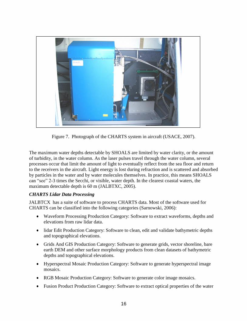
Figure 7. Photograph of the CHARTS system in aircraft (USACE, 2007).

The maximum water depths detectable by SHOALS are limited by water clarity, or the amount

of turbidity, in the water column. As the laser pulses travel through the water column, several

processes occur that limit the amount of light to eventually reflect from the sea floor and return

to the receivers in the aircraft. Light energy is lost during refraction and is scattered and absorbed

by particles in the water and by water molecules themselves. In practice, this means SHOALS

can “see” 2-3 times the Secchi, or visible, water depth. In the clearest coastal waters, the

maximum detectable depth is 60 m (JALBTXC, 2005).

CHARTS Lidar Data Processing

JALBTCX has a suite of software to process CHARTS data. Most of the software used for

CHARTS can be classified into the following categories (Sarnowski, 2006):

Waveform Processing Production Category: Software to extract waveforms, depths and

elevations from raw lidar data.

lidar Edit Production Category: Software to clean, edit and validate bathymetric depths

and topographical elevations.

Grids And GIS Production Category: Software to generate grids, vector shoreline, bare

earth DEM and other surface morphology products from clean datasets of bathymetric

depths and topographical elevations.

Hyperspectral Mosaic Production Category: Software to generate hyperspectral image

mosaics.

RGB Mosaic Production Category: Software to generate color image mosaics.

Fusion Product Production Category: Software to extract optical properties of the water

17

column and the bottom by fusion data from the bathymetric lidar and hyperspectral

radiometer and subsequently to characterize environment.

Survey Management Category: Software to manage mission planning for the SHOALS

system.

Metadata Management Category: Software to manage metadata files for final products.

The vendor of the SHOALS system is Optech Inc. whom also provides JABLTCX with a

Ground Control System (GCS) software package for post-mission data processing. The

Download module in GCS transfers the raw lidar data (INH, INT, IMG, POS, mission flight

plan, and log file) from a removable hard drive (used in the aircraft) to a desktop. The Automatic

Processing module processes waveform data from the INH files (the input hydrographic file) and

INT (the input topographic file) to generate depths and altitudes values. The result of Automatic

Processing is given in the form of HOF (hydrographic) and TOF (topographic output) files.

The following is summarized from (Sarnowski, 2006):

The Automatic Processing step requires also that the position orientation data is

made available. The raw data from INS and GPS are processed using software

recommended by manufactures of the INS and GPS units. The preparation of GPS

data includes appropriate processing of data from the additional ground GPS

stations or the C¬NAV receiver.

The module DAVIS of Optech's GCS integrates Fledermaus 3D from IVS3D Inc.

Fledermaus 3D is a software that allows a user to interactively clean, edit, validate

and 3D-visualize survey data in a 3D-environment. The Area Based Editor (ABE)

is a cleaning, editing and validating software developed in-house by

NAVOCEANO. Both editing software packages provide users with highly

interactive visualization techniques to validate large sets of point data (depths or

elevations) given in HOF and TOF files.

The primary preparation step is organization of point data records (from a

collection of flight lines) into of a 2-dimensional binned structure called a Pure

File Magic (PFM) dataset. After generating a PFM dataset, users interactively

validate depths or elevations. The validation step is very time consuming. As the

outcome of data validation process, the validation flags are set for point data

records in the PFM dataset as well as in the corresponding data sources (HOF and

TOF files).

The Project Mode of operation in GCS/DAVIS is used to process lidar datasets

from multiple missions. These datasets have to be already processed in the

Standalone Mode. The user has the ability to selectively choose (commit) which

flight-line to include in the project, based on the previous work in the standalone

mode. Both the raw lidar files and derived HOF and TOF files are committed. A

single PFM is built. After committing all required flight lines, the user will do in-

depth data validation and cleaning in Fledermaus (and ABE, if necessary). If

needed, the user will cycle many times between steps of selectively applying

positional corrections, re-running Automatic Processing , rebuilding the PFM, and

editing in Fledermaus (or ABE). The results of cleaning and validation are saved

into HOF and TOF files.

18

Cleaned lidar datasets are used by USACE to generate various hydrographic and

topographic grid products as TIN grids or DEM grids, the bare earth DEM grids

or specialized vector information as a zero contour to map the shoreline boundary.

From cleaned flight dataset, XYZ coordinates are extracted for points in an area

of interest, usually a 5 km length area block along a coast, using the custom 5km

Area Block Selection Program. If it is necessary, the geographical positions and

dimension units are transformed appropriately using various USACE software

(Wozencraft, et al, 2002).

The QT Modeler software is used to generate various grids and GeoTIFF images.

Topographic and GIS data processing applications as ArcMap, ArcView and

Lidar Analyst are used to generate specialized raster and vector products.

19

The Leica ALS50-II System

ALS50-II is a compact lidar system designed for the acquisition of topographic and return signal

intensity data from a variety of airborne platforms (Figure 8). The system is operated by 3001

Inc. of Slidell, LA. The data are computed using range and return signal intensity measurements

recorded in flight along with position and attitude data derived from airborne GPS and inertial

subsystems. By measuring the location (latitude, longitude and altitude) and attitude (roll pitch

and heading) of the aircraft, the distance to ground and scan angle (with respect to the base of the

scanner housing), a ground position for the impact point of each laser pulse can be determined.

The ALS50-II system is configured to include the following (Leica, 2008):

Specification for the Leica ALS50-II system reproduced below from http://www.leica-

geosystems.com/no/no/lgs_57629.htm:

Large-aperture low-inertia/high speed scan mirror: The standard scan mirror

is designed for use at altitudes up to 6000 m AGL at fields of view (FOV) to 75

degrees. The Scanner Assembly produces controlled movement of the transceiver

aim point by galvanometer actuation of a scan mirror. The aim point of the laser

output (relative to the scanner housing) is measured by a high accuracy optical

encoder. The scanner is a sealed, desiccated volume with a rigid optical window.

Laser Transmitter: The laser transmitter produces output laser pulses using a

diode-pumped transmitter. It also contains an optical trigger output optic, shutter,

and beam expansion/collimating optics that bring the laser output to the scan

mirror.

Receiver: The receiver collects a sample of the laser output pulse and detects

laser pulses reflected by the terrain below the aircraft.

Scanner Mechanization: A high-performance galvanometer scanner is used to

actuate the scan mirror.

Digital Camera: An XGA-resolution digital camera is included in the scanner.

This integrated camera allows a real-time view of the terrain below the aircraft, as

well as providing recorded images at fixed intervals. The recorded images

contain embedded annotation data. Leica LCam Viewer software allows the user

to search for a particular frame by GPS time, enabling selection of the appropriate

frame for any given portion of the LIDAR mission, and accesses the embedded

annotation data in order to provide automatic north-up image orientation. Zoom

functions are also provided.

The recommended maximum slant range for the system is approximately 7563 m.

The system can be operated at longer slant ranges, though low-reflectivity targets

may not produce adequate signal for detection, resulting in “drop-outs” over areas

of low reflectivity, such as freshly-paved asphalt. The scan rate is user-selectable

from 0 to 90 Hz in 0.1 Hz increments via the graphical user interface. System

control software prevents out-of-range inputs for scan rate based on user selection

20

for FOV. The ALS50-II system provides a sinusoidal scan pattern in a plane

nominally orthogonal to the longitudinal axis of the scanner, nominally centered

about nadir. The illuminated footprint beam divergence is 0.22 mr nominal,

measured at the 1/e2 point. For reference, this is equivalent to 0.15 mr measured

at the 1/e point.

Figure 8. The ALS50 lidar system (Leica, 2008).

The ALS50-II system produces data after post processing with a lateral placement accuracy of 7

– 64 cm and vertical placement accuracy of 8 - 24 cm (one standard deviation) from full-field-

filling targets of 10 percent diffuse reflectivity or greater with atmospheric visibility of 23.5 km

or better for flying heights up to 6000 m AGL and nominal FOV of 40 degrees (Leica,

http://www.leica-geosystems.com/no/no/lgs_57629.htm, 2008)

ALS50-II Data Processing

Data processing for the ALS540 is described a metadata file “Louisiana Barrier Island LiDAR

Survey, (USACE, 2007):

The ABGPS, IMU, and raw scans are integrated using proprietary software

developed by the Leica Geosystems and delivered with the Leica ALS50 System.

The resultant file is in a LAS binary file format. The LAS file format can be

easily transferred from one file format to another. It is a binary file format that

maintains information specific to the LiDAR data (return#, intensity value, xyz,

etc.). The resultant points are produced in the State Plane Louisiana South

21

coordinate system (FIPS 1702), with units in feet and referenced to the NAD83

horizontal datum and NAVD88 vertical datum.

Filtered and edited data are subjected to rigorous QA/QC according to the 3001

Inc. Quality Control Plan and procedures. A series of quantitative and visual

procedures are employed to validate the accuracy and consistency of the filtered

and edited data. Ground control is established by 3001, Inc. and GPS-derived

ground control points (GCPs) points in various areas of dominant and prescribed

land cover. These points are coded according to landcover, surface material and

ground control suitability. A suitable number of points are selected for calculation

of a statistically significant accuracy assessment as per the requirements of the

National Standard for Spatial Data Accuracy. A spatial proximity analysis is used

to select edited LIDAR data points within a specified distance of the relevant

GCPs. A search radius decision rule is applied with consideration of terrain

complexity, cumulative error and adequate sample size. Accuracy validation and

evaluation is accomplished using proprietary software to apply relevant statistical

routines for calculation of Root Mean Square Error (RMSE) and the National

Standard for Spatial Data Accuracy (NSSDA) according to Federal Geographic

Data Committee (FGDC) specifications.

The accuracy of the ALS50-II data was assessed by comparing ground truth

checkpoints with ALS50-II points from the edited data set, which were within 1

meter, horizontally from the ground truth points. The only exception to this were

the ground truth points collected under tree canopy, where comparisons were

made with ALS50-II points that fell within 3 meters of the check points. This is

because fewer ALS50-II pulses are able to reach the ground in heavily forested

areas, so the point spacing is not as dense as the point spacing in cleared areas.

Note that the edited ALS50-II points are simply a subset of the raw ALS50-II

points. The points that fell above the ground surface on vegetation canopies,

buildings, or other obstructions were removed from the data set. The result of the

comparison of these values indicated a Vertical Root Mean Square Error (RMSE)

of less than 15 centimeters, which equates to Vertical Accuracy of 30 centimeters

at the 95 percent confidence level.

22

USGS GRID PROCESSING TECHNIQUES

Basic Grid Processing

The grids included in this project were created using ESRI‟s ArcWorkstation 9.2 and are in

ArcInfo‟s standard grid format. In general, the xyz data were converted to points, the points

were used to make tins, and the tins converted to grids using linear interpolation. The “not

cleaned” grids in this package are the output of the tin to grid conversion. Grids were further

processed to remove open water and no-data areas. These “cleaned” grids are also included in

this package.

Grid Cleaning

Cleaning steps included removing no-data areas, removing areas falling below a certain elevation

approximating mean high water level, and hand cleaning. The tinning process creates false data,

particularly around the exterior of the data collection area. Removing no-data areas eliminates

most of the false data. Removing areas falling below an elevation that approximates mean high

water usually removes most of the open water and often removes lakes/ponds. When water

levels were high, higher elevations were used to remove open water areas. Hand cleaning

removed remaining open water areas.

Cleaning the grids for the Chandeleur Islands was handled somewhat differently than for the rest

of Louisiana. They are low lying and contain many small lakes and ponds and other relatively

small features. First surface grids smoothed with a 3 meter x 3 meter neighborhood mean were

used to determine approximate shorelines and land areas for each survey. Lakes and ponds

below the elevation used to remove open water and with areas greater than or equal to 25 meters2

were removed. Extensive hand-editing was necessary to remove open water in some of the

surveys. Once the first surface land areas were identified, they were used to make the cleaned

grids from the unsmoothed first surface and bare earth grids.

The first surface and bare earth grids in the remainder of Louisiana were cleaned separately. The

grids were smoothed with a 3 meter x 3 meter neighborhood mean. Elevations below an

approximate mean high water level of .37 meters were removed. Minor hand editing removed

remaining open water areas. Interior areas of no-data larger than 500 meters2

were removed.

Interior areas with elevations below .37 meters and larger than 500 meters2

were removed. The

cleaned grids contain the smoothed data.

Difference (Change) Grids

Difference (or change) grids were made by subtracting the older cleaned grid from the more

recent cleaned grid. This results in negative values in areas where elevations decreased over

time and positive values where elevations increased over time. Only those areas that have data

in both survey‟s cleaned grids have values in the difference grids.

23

REFERENCES

Brock, J.C., Wright, C.W., Sallenger, A.H., Krabill, W.B., and R.N. Swift, 2002, Basis and

methods of NASA Airborne Topographic Mapper Lidar surveys for coastal studies, Journal of

Coastal Research, Vol. 18, No. 1, p. 1-13.

JALBTCX, 2005, Standard Operating Proceedures, U. S. Army Corps of Enginerers, Joint

Airborne Lidar Bathymetry Technical Center of Expertise (JALBTCX), 16pp.

Leica, 2008, Leica ALS50-II Airborne Laser Scanner Product Specifications, Leica Geosystems

AG, Heerbrugg, Switzerland, 2007.

Nayegandhi, A., 2001, Lasermap: Processing System for Lidar Imagery, Master‟s Thesis,

University of South Florida, pp.87.

Nayegandhi, A., Brock, J.C., In Press. Assessment of coastal-vegetation habitats using airborne

laser remote sensing. To be published as a book chapter in "Remote Sensing and Spatial

Information Technologies for Coastal Ecosystem Assessment and Management: Principles and

Applications" Springer Publication.

Nayegandhi, A., Brock, J.C., Wright, C.W., In Press. Small-footprint, waveform-resolving lidar

estimation of submerged and sub-canopy topography in coastal environments. International

Journal of Remote Sensing.

Optech Inc., 2008, http://www.optech.ca/pdf/Brochures/SHOALS2007.pdf

Sarnowski ,Krzysztof, 2006, Processing Software at JABLTCX and Processing Acceleration

Opportunities, University Of Southern Mississippi, Hydrographic Research Science Center,

Stennis Space Center, MS, pp35.

USACE, 2007, Louisiana Barrier Islands LiDar Survey (Metadata), U.S. Army Corps of

Engineer District, Mobile, pp14.

Wright, C.W. and J. Brock, 2002, EAARL: A lidar for mapping shallow coral reefs and other

coastal environments, Paper in the Proceedings of the Seventh International Conference on

Remote Sensing for Marine and Coastal Environments, Miami, 20-22, May 2002.

Wozencraft, J.M., Lillycrop, W.J. and Kraus, N.C. 2002. SHOALS Toolbox: software to support

visualization and analysis of large, high-density data sets. ERDC/CHL-CHETN-IV-43, U.S.

Army Engineer Research and Development Center, Vicksburg, MS.