1

Robust Odometry and Mapping for Multi-LiDARSystems with Online Extrinsic Calibration

Jianhao Jiao, Haoyang Ye, Yilong Zhu, and Ming Liu

Abstract—Combining multiple LiDARs enables a robot tomaximize its perceptual awareness of environments and obtainsufficient measurements, which is promising for simultaneous lo-calization and mapping (SLAM). This paper proposes a system toachieve robust and simultaneous extrinsic calibration, odometry,and mapping for multiple LiDARs. Our approach starts withmeasurement preprocessing to extract edge and planar featuresfrom raw measurements. After a motion and extrinsic initializa-tion procedure, a sliding window-based multi-LiDAR odometryruns onboard to estimate poses with an online calibrationrefinement and convergence identification. We further develop amapping algorithm to construct a global map and optimize poseswith sufficient features together with a method to capture andreduce data uncertainty. We validate our approach’s performancewith extensive experiments on ten sequences (4.60km total length)for the calibration and SLAM and compare them against thestate-of-the-art. We demonstrate that the proposed work isa complete, robust, and extensible system for various multi-LiDAR setups. The source code, datasets, and demonstrationsare available at: https://ram-lab.com/file/site/m-loam.

Index Terms—Simultaneous localization and mapping, calibra-tion and identification, sensor fusion, autonomous driving.

I. INTRODUCTION

A. Motivation

S IMULTANEOUS Localization and Mapping (SLAM) isessential to a wide range of applications, such as scene

reconstruction, robotic exploration, and autonomous driving[1]–[3]. Approaches that use only a LiDAR have attractedmuch attention from the research community due to their accu-racy and reliability in range measurements. However, LiDAR-based methods commonly suffer from data sparsity and limitedvertical field of view (FOV) in real-world applications [4].For instance, LiDARs’ points distribute loosely, which inducesa mass of empty regions between two nearby scans. Thischaracteristic usually causes state estimation to degeneratein structureless environments, such as narrow corridors andstairs [5]. Recently, owing to the decreasing price of sensors,we have seen a growing trend of deploying multi-LiDARsystems on practical robotic platforms [6]–[11]. Comparedwith a single-LiDAR setup, the primary improvement of multi-LiDAR systems is the significant enhancement on the sensingrange and density of measurements. This benefit is practically

This work was supported by Collaborative Research Fund by ResearchGrants Council Hong Kong, under Project No. C4063-18G, Department ofScience and Technology of Guangdong Province Fund, under Project No.GDST20EG54 and Zhongshan Municipal Science and Technology BureauFund, under project ZSST21EG06, awarded to Prof. Ming Liu.

The authors are with the Department of Electrical and Computer Engineer-ing, Hong Kong University of Science and Technology, Hong Kong, China(email: {jjiao, hyeab, yzhubr}@connect.ust.hk, eelium@ust.hk).

useful for self-driving cars since we have to address the criticalblind spots created by the vehicle body. Thus, we considermulti-LiDAR systems in this paper.

B. Challenges

Despite their great advantages in environmental perception,a number of issues affect the development of SLAM using amulti-LiDAR setup.

1) Precise and Flexible Extrinsic Calibration: Recoveringthe multi-LiDAR transformations for a new robotic platformis complicated. In many cases, professional users have tocalibrate sensors in human-made surroundings [12] carefully.This requirement increases the cost to deploy and maintain amulti-LiDAR system for field robots.

It is desirable that the system can self-calibrate the ex-trinsics in various environments online. As shown in [13]–[15], benefiting from the simultaneous estimation of extrinsicsand ego-motion, the working scope of visual-inertial sys-tems has been expanded to drones and vessels in outdoorscenes. These approaches continuously perform calibrationduring the mission to guarantee the objective function tobe always ‘optimal’. However, this process typically requiresenvironmental or motion constraints to be fully observable.Otherwise, the resulting extrinsics may become suboptimalor unreliable. Thus, we have to fix the extrinsics if theyare accurate, which creates a demand for online calibrationwith a convergence identification. In order to cope with thecentimeter-level calibration error and unexpected changes onextrinsics over time, it is also beneficial to model the extrinsicperturbation for multi-LiDAR systems.

2) Low Pose Drift: To provide accurate poses in realtime, state-of-the-art (SOTA) LiDAR-based methods [16]–[18]commonly solve SLAM by two algorithms: odometry andmapping. These algorithms are designed to estimate posesin a coarse-to-fine fashion. Based on the original odometryalgorithm, an approach that fully exploits multi-LiDAR mea-surements within a local window is required. The increasingconstraints help to prevent degeneracy or failure of frame-to-frame registration. The subsequent mapping algorithm runsat a relatively low frequency and is given plenty of featurepoints and many iterations for better results. However, as weidentify in Section VIII, many SOTA approaches neglect thefact that uncertain points in the global map limit the accuracy.To minimize this adverse effect, we must develop a methodto capture map points’ uncertainties and reject outliers.

arX

iv:2

010.

1429

4v2

[cs

.RO

] 5

May

202

1

2

C. Contributions

To tackle these challenges, we propose M-LOAM, a ro-bust system for Multi-LiDAR extrinsic calibration, real-timeOdometry, and Mapping. Without manual intervention, oursystem can start with several extrinsic-uncalibrated LiDARs,automatically calibrate their extrinsics, and provide accurateposes as well as a globally consistent map. Our previouswork [5] proposed sliding window-based odometry to fuseLiDAR points with high-frequency IMU measurements. Thatframework inspires this paper, where we try to solve theproblem of multi-LiDAR fusion. In addition, we introduce amotion-based approach [4] to initialize extrinsics, and employthe tools in [19] to represent uncertain quantities. Our designof M-LOAM presents the following contributions:

1) Automatic initialization that computes all critical states,including motion between consecutive frames as well asextrinsics for subsequent phases. It can start at arbitrarypositions without any prior knowledge of the mechanicalconfiguration or calibration objects (Section VI).

2) Online self-calibration with a general convergence crite-rion is executed simultaneously with the odometry. It hasthe capability to monitor the convergence and trigger ter-mination in a fully unsupervised manner (Section VII-B).

3) Sliding window-based odometry that fully exploits in-formation from multiple LiDARs. This implementationcan be explained as small-scale frame-to-map registra-tion, which further reduces the drift accumulated by theconsecutive frame-to-frame odometry (Section VII-C).

4) Mapping with a two-stage approach that captures andpropagates uncertain quantities from sensor noise, de-generate pose estimation, and extrinsic perturbation. Thisapproach enables the mapping process with an awarenessof uncertainty and helps us to maintain the consistency ofa global map as well as boost the robustness of a systemfor long-duration navigation tasks (Section VIII).

To the best of our knowledge, M-LOAM is the first completesolution to multi-LiDAR calibration and SLAM. The systemis evaluated under extensive experiments on both handhelddevices and autonomous vehicles, covering various scenariosfrom indoor offices to outdoor urban roads, and outperformsthe SOTA LiDAR-based methods. Regarding the calibration ondiverse platforms, our approach achieves an extrinsic accuracyof centimeters in translation and deci-degrees in rotation. Forthe SLAM in different scales, M-LOAM has been successfullyapplied to provide accurate poses and map results. Fig. 1visualizes M-LOAM’s output at each stage. To benefit theresearch community, we publicly release our code, implemen-tation details, and the multi-LiDAR datasets.

D. Organization

The rest of the paper is organized as follows. SectionII reviews the relevant literature. Section III formulates theproblem and provides basic concepts. Section IV gives theoverview of the system. Section V describes the preprocessingmodule on LiDAR measurements. Section VI introduces themotion and extrinsic initialization procedure. Section VII

Trajectory of Odometry

Trajectory of Mapping

LiDAR MapCalibration

Raw LiDAR point clouds

Measurement Preprocessing

Extracted features

LiDAR 1

LiDAR 2

LiDAR 1

LiDAR 2

Fig. 1. We visualize the immediate results of M-LOAM. The raw point cloudsperceived by different LiDARs are denoised and extracted with edge (bluedots) and planar (red dots) features, which are shown at the top-right position.The proposed online calibration is performed to obtain accurate extrinsics.After that, the odometry and mapping algorithms use these features to estimateposes. The trajectory of the mapping (green) is more accurate than that of theodometry (red).

presents the tightly coupled, sliding window-based multi-LiDAR odometry (M-LO) with online calibration refinement.The uncertainty-aware multi-LiDAR mapping algorithm isintroduced in Section VIII, followed by experimental resultsin Section IX. In Section X, we provide a discussion aboutthe proposed system. Finally, Section XI concludes this paperwith possible future research directions.

II. RELATED WORK

Scholarly works on SLAM and extrinsic calibration areextensive. In this section, we briefly review relevant resultson LiDAR-based SLAM and online calibration methods formulti-sensor systems.

A. LiDAR-Based SLAM

Generally, many SOTA are developed from the iterativeclosest point (ICP) algorithm [20]–[23], into which the meth-ods including measurement preprocessing, degeneracy predic-tion, and sensor fusion are incorporated. These works havepushed the current LiDAR-based systems to become fast,robust, and feasible to large-scale environments.

1) Measurement Preprocessing: As the front-end of a sys-tem, the measurement preprocessing encodes point clouds intoa compact representation. We categorize related algorithmsinto either dense or sparse methods. As a typical dense method,SuMa [24] demonstrates the advantages of utilizing surfel-based maps for registration and loop detection. Its extendedversion [25] incorporates semantic constraints into the originalcost function. The process of matching dense pixel-to-pixelcorrespondences make the method computationally intensive,

3

thus requiring dedicated hardware (GPU) for real-time oper-ation. These approaches are not applicable to our cases sincewe have to frequently perform the registration on a CPU.

Sparse methods prefer to extract geometric features fromraw measurements and are thus supposed to have real-timeperformance. Grant et al. [26] proposed a plane-based reg-istration, while Velas et al. [27] represented point clouds ascollar line segments. Compared to them, LOAM [16] has fewerassumptions about sensors and surroundings. It selects distinctpoints from both edge lines and local planar patches. Recently,several following methods have employed ground planes [17],[28], visual detection [29], probabilistic grid maps [30], goodfeatures [31], or directly used dense scanners [18], [32], [33]to improve the performance of sparse approaches in noisyor structure-less environments. To limit the computation timewhen more LiDARs are involved, we extract the sparse edgeand planar features like LOAM. But differently, we representtheir residuals in a more concise and unified way.

2) Degeneracy in State Estimation: The geometric con-straints of features are formulated as a state estimation prob-lem. Different methods have been proposed to tackle thedegeneracy issue. Zhang et al. [34] defined a factor, whichis equal to the minimum eigenvalue of information matrices,to determine the system degeneracy. They also proposed atechnique called solution remapping to update variables inwell-conditioned directions. This technique was further ap-plied to tasks including localization, registration, pose graphoptimization, and inspection of sensor failure [35]–[37]. Toquantify a nonlinear system’s observability, Rong et al. [38]computed the condition number of the empirical observabilityGramian matrix. Since our problem linearizes the objectivefunction as done in Zhang et al. [34], we also introducesolution remapping to update states. Additionally, our onlinecalibration method employs the degeneracy factor as a quan-titative metric of the extrinsic calibration.

3) Multi-Sensor Fusion: Utilizing multiple sensors toimprove the motion-tracking performance of single-LiDARodometry is promising. Most existing works on LiDAR-basedfusion combine visual or inertial measurements. The simplestway to deal with multi-modal measurements is loosely coupledfusion, where each sensor’s pose is estimated independently.For example, LiDAR-IMU fusion is usually done by theextended Kalman filter (EKF) [39]–[41]. Tightly coupledalgorithms that optimize sensors’ poses by jointly exploitingall measurements have become increasingly prevalent in thecommunity. They are usually done by either the EKF [42]–[44] or batch optimization [5], [45]–[48]. Besides multi-modalsensor fusion, another approach is to explore the fusion ofmultiple LiDARs (uni-model), which is still an open problem.

Multiple LiDARs improve a system by maximizing thesensing coverage against extreme occlusion. Inspired by thesuccess of tightly coupled algorithms, we achieve a slidingwindow estimator to optimize states of multiple LiDARs. Thismode has great advantages for multi-LiDAR fusion.

B. Multi-Sensor CalibrationPrecise extrinsic calibration is important to any multi-

sensor system. Traditional methods [12], [49]–[51] have to

run an ad-hoc calibration procedure before a mission. Thistedious process needs to be repeated whenever there is slightperturbation on the structure. A more flexible solution to esti-mate these parameters is combined SLAM-based techniques.Here, extrinsics are treated as one of the state variables andoptimized along with sensors’ poses. This scheme is alsoapplicable to some non-stationary parameters, such as robotkinematics, IMU biases, and time offsets.

Kummerle et al. [52] pioneered a hyper-graph optimizationframework to calibrate an onboard laser scanner with wheelencoders. Their experiments reveal that online correction ofparameters leads to consistent and accurate results. Teichmanet al. [53], meanwhile, proposed an iterative SLAM-fittingpipeline to resolve the distortion of two RGB-D cameras.To recover spatial offsets of a multi-camera system, Henget al. [54] formulated the problem as a bundle adjustment,while Ouyang et al. [55] employed the Ackermann steeringmodel of vehicles to constrain extrinsics. As presented in[47], [56]–[58], the online estimation of time offsets amongsensors is crucial to IMU-centric systems. Qin et al. [56]utilized reprojection errors of visual features to formulate thetemporal calibration problem, while Qiu et al. [58] proposeda more general method to calibrate heterogeneous sensors byanalyzing sensors’ motion correlation.

This paper implicitly synchronizes the time of multipleLiDARs with an hardware-based external clock and explicitlyfocuses on the extrinsic calibration. Our approach consists ofan online procedure to achieve flexible multi-LiDAR extrinsiccalibration. To monitor the convergence of estimated extrin-sics, we propose a general criterion. In addition, we model theextrinsic perturbation to reduce its negative effect for long-term navigation tasks.

III. PROBLEM STATEMENT

We formulate M-LOAM in terms of the Maximum Like-lihood Estimation (MLE). The MLE leads to a nonlinearoptimization problem where the inverse of the Gaussian co-variances weights the residual functions. Before delving intodetails of M-LOAM, we first introduce some basic concepts.Section III-A presents notations. Section III-B introduces theMLE, and Section III-C describes suitable models to representuncertain measurements in R3 and transformations in SE(3).Finally, Section III-D briefly presents the implementation ofthe MLE with approximate Gaussian noise in M-LOAM.

A. Notations and Definitions

The nomenclature is shown in Table I. We consider a systemthat consists of one primary LiDAR and multiple auxiliaryLiDARs. The primary LiDAR defines the base frame, and weuse ()l

1

/()b to indicate it. The frames of the auxiliary LiDARsare denoted by ()l

i,i>1

. We denote F as the set of availablefeatures extracted from the LiDARs’ raw measurements. Eachfeature is represented as a point in 3D space: p = [x, y, z]>.The state vector, composed of translational and rotationalparts, is denoted by x = [t,q] where t is a 3× 1 vector, andq is the Hamilton quaternion. But in the case that we needto rotate a vector, we use the 3 × 3 rotation matrix R in the

4

Lie group SO(3). We can convert q into R with the Rodriguesformula [59]. Section VIII associates uncertainty with poses onthe vector space, where we use the 4×4 transformation matrixT in the Lie group SE(3) to represent a pose. A rotation matrixand translation vector can be associated with a transformationmatrix as T =

[R p0> 1

].

B. Maximum Likelihood EstimationWe formulate the pose and extrinsic estimation of a multi-

LiDAR system as an MLE problem [60]:

xk = arg maxxk

p(Fk|xk) = arg minxk

f(xk,Fk), (1)

where Fk represents the available features at the kth frame,xk is the state to be optimized, and f(·) is the objectivefunction. Assuming the measurement model to be subjectedto Gaussian noise [3], problem (1) becomes a nonlinear least-squares (NLS) problem:

xk = arg minxk

m∑i=1

ρ(∣∣∣∣r(xk,pki)

∣∣∣∣2Σi

), (2)

where ρ(·) is the robust Huber loss to handle outliers [61],r(·) is the residual function, and Σi is the covariance ma-trix. Iterative methods such as Gauss-Newton or Levenberg-Marquardt can offen be used to solve this NLS problem. Thesemethods locally linearize the objective function by computingthe Jacobian w.r.t. xk as J = ∂f/∂xk. Given an initial guess,xk is iteratively optimized by usage of J until convergingto a local minima. At the final iteration, the least-squarescovariance of the state is calculated as Ξ = Λ−1 [62], whereΛ = J>J is called the information matrix.

C. Uncertainty RepresentationWe employ the tools in [19] to represent data uncertainty.

We first represent a noisy LiDAR point as

p = p + ζ, ζ ∼ N (0,Z), (3)

where p is a noise-free vector, ζ ∈ R3 is a small Gaussianperturbation variable with zero mean, and Z is a noise covari-ance of LiDAR measurements. To make (3) compatible withtransformation matrices (i.e., p′h = Tph), we also express itwith 4× 1 homogeneous coordinates:

ph =

[p1

]+ Dζ = ph + Dζ, ζ ∼ N (0,Z), (4)

where D is a matrix that converts a 3 × 1 vector into ho-mogeneous coordinates. As investigated in [63], the LiDARs’depth measurement error (also called sensor noise) is primarilyaffected by the target distances. Z is simply set as a constantmatrix.1 We then define a random variable in SE(3) with asmall perturbation according to2

T = exp(ξ∧)T, ξ ∼ N (0,Ξ), (5)

1Z = diag(σ2x, σ

2y , σ

2z), where σx, σy , σz are standard deviations of

LiDARs’ depth noise along different axes. We refer to manuals to obtainthem for a specific LiDAR.

2The (·)∧ operator turns ξ into a member of the Lie algebra se(3). Theexponential map associates an element of se(3) to a transformation matrix inSE(3). Similarly, we can also use (·)∧ and exp(·) to associate 3× 1 vectorφ with a rotation matrix in SO(3). [19] provides detailed expressions.

TABLE INOMENCLATURE

Notation Explanation

Coordinate System and Pose Representation

()w, ()b, ()li

Frame of the world, primary sensor, and ith LiDAR()l

ik Frame of the ith LiDAR while taking the kth point cloudI Number of LiDARs in a multi-LiDAR system

p, ph 3D Point in R3 and homogeneous coordinatesx State vectort Translation vector in R3

q Hamilton quaternionR Rotation matrix in the Lie group SO(3)T Transformation matrix in the Lie group SE(3)

ξ, ζ,θ Gaussian noise variableΣ Covariance matrix of residualsZ Covariance matrix of LiDAR depth measurement noiseΞ Covariance matrix of pose noise

Odometry and Mapping

F Features extracted from raw point cloudsE,H Edge and planar subset of extracted featuresL,Π Edge line and planar patch[w, d] Coefficient vector of a planar patchM Local mapG Global mapλ Degeneracy factor

where T is a noise-free transformation and ξ ∈ R6 is the smallperturbation variable with covariance Ξ. This representationallows us to store the mean transformation as T and use ξ forperturbation on the vector space. We consider that Ξ indicatestwo practical error sources:• Degenerate Pose Estimation arises from cases such

as lack of geometrical structures in poorly constrainedenvironments [34]. It typically makes poses uncertainin their degenerate directions [62], [64]. Existing worksresort to model-based and learning-based [65] methodsto estimate pose covariances in the context of ICP. orvibration, impact, and temperature drift during long-termoperation.

• Extrinsic Perturbation always exists due to calibrationerrors [12], Wide baseline sensors such as stereo cameras,especially, suffer even more extrinsic deviations thanstandard sensors. Such perturbation is detrimental to themeasurement accuracy [66], [67] of multi-sensor systemsbut is hard to measure.

The computation of Ξ is detailed in Section VIII.

D. MLE with Approximate Gaussian Noise in M-LOAM

We extend the MLE to design multiple M-LOAM estima-tors to solve the robot poses and extrinsics in a coarse-to-fine fashion. The most important step is to approximate theGaussian noise covariance Σ to realistic measurement models.Based on the discussion in Section III-C, we identify thatthree sources of error may make landmarks uncertain: sensornoise, degenerate pose estimation, and extrinsic perturbation.The frame-to-frame motion estimation (Section VI-A) is ap-proximately subjected to the sensor noise. The tightly coupledodometry (Section VII-C) establishes a local map for the poseoptimization. We should propagate pose uncertainties onto

5

LiDAR 1 (10Hz)

LiDAR 2 (10Hz)

LiDAR 3 (10Hz)

Measurement Preprocessing (Section V) Initialization (Section VI)

Initialized?

Yes

Segmentation for

Noise Removal

Feature Extraction

and Matching

Frame-to-Frame

Motion Estimation

Linear Rotation

and Translation

Calibration

Oldest Sliding Window Newest

Optimization with

Online Calibration

Optimization with

Pure Odometry

Calibrated?

Yes

Multi-LiDAR Odometry with Calibration Refinement (Section VII)Multi-LiDAR Mapping (Section VIII)

Uncertainty Estimation

and Propagation

Uncertainty-Aware

OperationNo

Monitoring the

Convergence

No

Fig. 2. The block diagram illustrating the full pipeline of the proposed M-LOAM system. The system starts with measurement preprocessing (Section V).The initialization module (Section VI) initializes values for the subsequent nonlinear optimization-based multi-LiDAR odometry with calibration refinement(Section VII). According to the convergence of calibration, the optimization is divided into two subtasks: online calibration and pure odometry. If the calibrationconverges, we can skip the extrinsic initialization and refinement steps, and enter the pure odometry and mapping phase. The uncertainty-aware multi-LiDARmapping (Section VIII) maintains a globally consistent map to decrease the odometry drift and remove noisy points.

each map point. Nevertheless, this operation is often time-consuming (around 10ms−20ms) if more LiDARs and slidingwindows are involved. To guarantee the real-time odometry,we do not compute the pose uncertainty here. We simplyset Σ = Z as the covariance of residuals. In mapping, weare given sufficient time for an accurate pose and a globalmap. Therefore, we consider all uncertainty sources. SectionVIII explains how the pose uncertainty affects the mappingprecision and Σ is propagated.

IV. SYSTEM OVERVIEW

We make three assumptions to simplify the system design:

• LiDARs are synchronized, meaning that the temporallatency among different LiDARs is almost zero.

• The platform undergoes sufficient rotational and transla-tional motion in the period of calibration initialization.

• The local map of the primary LiDAR should sharean overlapping FOV with auxiliary LiDARs for featurematching in refinement to shorten the calibration phase.This can be achieved by moving the robot.

Fig. 2 presents the pipeline of M-LOAM. The system startswith measurement preprocessing (Section V), in which edgeand planar features are extracted and tracked from denoisedpoint clouds. The initialization module (Section VI) providesall necessary values, including poses and extrinsics, for boot-strapping the subsequent nonlinear optimization-based M-LO.The M-LO fuses multi-LiDAR measurements to optimizethe odometry and extrinsics within a sliding window. If theextrinsics already converge, we skip the extrinsic initializationas well as refinement steps and enter the pure odometry andmapping phase. The probabilistic mapping module (SectionVIII) constructs a global map with sufficient features toeliminate the odometry drift. The odometry and mapping runconcurrently in two separated threads.

V. MEASUREMENT PREPROCESSING

We implement three sequential steps to process LiDARs’raw measurements. We first segment point clouds into manyclusters to remove noisy objects, and then extract edge andplanar features. To associate features between consecutiveframes, we match a series of correspondences. In this section,each LiDAR is handled independently.

A. Segmentation for Noise Removal

With knowing the vertical scanning angles of a LiDAR, wecan project the raw point cloud onto a range image withoutdata loss. In the image, each valid point is represented by apixel. The pixel value records the Euclidean distance froma point to the origin. We apply the segmentation methodproposed in [68] to group pixels into many clusters. Weassume that two neighboring points in the horizontal or verticaldirection belong to the same object if their connected lineis roughly perpendicular (> 60deg) to the laser beam. Weemploy the breadth-first search algorithm to traverse all pixels,ensuring a constant time complexity. We discard small clusterssince they may offer unreliable constraints in optimization.

B. Feature Extraction and Matching

We are interested in extracting the general edge and planarfeatures. We follow [16] to select a set of feature pointsfrom measurements according to their curvatures. The set ofextracted features F consists of two subsets: edge subset (highcurvature) E and planar subset (low curvature) H. Both Eand H consist of a portion of features which are the mostrepresentative. We further collect edge points from E with thehighest curvature and planar points from H with the lowestcurvature. These points form two new sets: E and H. Thenext step is to determine feature correspondences betweentwo consecutive frames, ()l

ik−1 → ()l

ik , to construct geometric

constraints. For each point in E lik , two closest neighbors fromE l

ik−1 are selected as the edge correspondences. For a point in

6

Corresponding planar point

Planar point

Corresponding edge point

Edge point

Fig. 3. The planar and edge residuals. The red dot indicates the referencepoint and the green dots are its corresponding points.

Hlik , the three closest points to Hlik−1 that form a plane are

selected as the planar correspondences.

VI. INITIALIZATION

Optimizing states of multiple LiDARs is highly nonlinearand needs initial guesses. This section introduces our motionand extrinsic initialization approach, which does not requireany prior mechanical configuration of the sensor suite. It alsodoes not involve any manual effort, making it particularlyuseful for autonomous robots.

A. Scan-Based Motion Estimation

With found correspondences between two successive framesof each LiDAR, we estimate the frame-to-frame transforma-tion by minimizing residual errors of all features. As illustratedin Fig. 3, the residuals are formulated by both edge andplanar correspondences. Let xk be the relative transformationbetween two scans of a LiDAR at the kth frame. Regardingplanar features, for a point p ∈ Hlik , if Π is the correspondingplanar patch, the planar residual is computed as

rH(xk,p,Π) = aw, a = w>(Rkp + tk) + d, (6)

where a is the point-to-plane Euclidean distance and [w, d] isthe coefficient vector of Π. Then, for an edge point p ∈ E lik , ifL is the corresponding edge line, we define the edge residualas a combination of two planar residuals using (6) as

rE(xk,p, L) =[rH(xk,p,Π1), rH(xk,p,Π2)

], (7)

where [w1, d1] and [w2, d2] are the coefficients of Π1 andΠ2, w1 coincides with the projection direction from L to p,and Π2 is perpendicular to Π1 s.t. w2⊥w1, and w2⊥L. Theabove definitions are different from that of LOAM [16], andshow two benefits. Firstly, the edge residuals offer additionalconstraints to the states. Furthermore, the residuals are repre-sented as vectors, not scalars, allowing us to multiply a 3× 3covariance matrix. We minimize the sum of all residual errorsto obtain the MLE as

xk = arg minxk

∑p∈Fli

k

ρ(∥∥rF (xk,p)

∥∥2Σp

),

rF (xk,p) =

{rE(xk,p, L) if p ∈ E likrH(xk,p,Π) if p ∈ Hlik

,

(8)

where the Jacobians of rF (·) are detailed in Appendix A.In practice, points are skewed after a movement on LiDARs

with a rolling-shutter scan. After solving the incrementalmotion xk, we correct points’ positions by transforming theminto the last frame ()l

ik−1 . Let tk−1 and tk be the start and end

time of a LiDAR scan respectively. For a point p captured att ∈ (tk−1, tk], it is transformed as3

plik−1 = Rτ

kp + tτk, τ =t− tk−1tk − tk−1

, (9)

where the rotation and translation are linearly interpolated [5]:

Rτk = exp(φ∧k )τ = exp(τφ∧k ), tτk = τtk. (10)

B. Calibration of Multi-LiDAR System

The initial extrinsics are obtained by aligning motion se-quences of two sensors. This is known as solving the hand-eye calibration problem AX = XB, where A and B arethe historical transformations of two sensors and X is theirextrinsics. As the robot moves, the following equations of theith LiDAR should hold for any k

Rlik−1

likRbli = Rb

liRbk−1

bk, (11)

(Rlik−1

lik− I3)tbli = Rb

litbk−1

bk− t

lik−1

lik, (12)

where the original problem is decomposed into the rotationaland translational components according to [14]. We implementthis method to initialize the extrinsics online.

1) Rotation Initialization: We rewrite (11) as a linearequation by employing the quaternion:

qlik−1

lik⊗ qbli = qbli ⊗ q

bk−1

bk

⇒[Q1(q

liklik−1

)−Q2(qbk−1

bk)]

qbli = Qk−1k qbli ,

(13)

where ⊗ is the quaternion multiplication operator and Q1(·)and Q2(·) are the matrix representations for left and rightquaternion multiplication [59]. Stacking (13) from multipletime intervals, we form an overdetermined linear system as w0

1 ·Q01

...wK−1K ·QK−1

K

4K×4

qbli = QKqbli = 04K×4, (14)

where K is the number of constraints, and wk−1k are robustweights defined as the angle in the angle-axis representationof the residual quaternion:

wk−1k = ρ′(φ), φ = 2 arctan(||qxyz||, qw

),

q = (qbli)∗ ⊗ (q

lik−1

lik)∗ ⊗ qbli ⊗ q

bk−1

bk,

(15)

where ρ′(·) is the derivative of the Huber loss, qbli is thecurrently estimated extrinsic rotation, and q∗ is the inverse ofq. Subject to ‖qbli‖ = 1, we find the closed-form solution of(14) using SVD. For the full observability of 3-DoF rotation,sufficient motion excitation are required. Under sufficientconstraints, the null space of QK should be rank one. This

3The timestampe of each point can be obtained from raw data.

7

Fixed state Variable or Extrinsic state Map-based measurements

Local map within the window of the base LiDAR

Local map within the window of the 𝑖𝑡ℎ LiDAR

The base

LiDAR

The 𝑖𝑡ℎ

LiDAR

Local map within the window of the base LiDAR

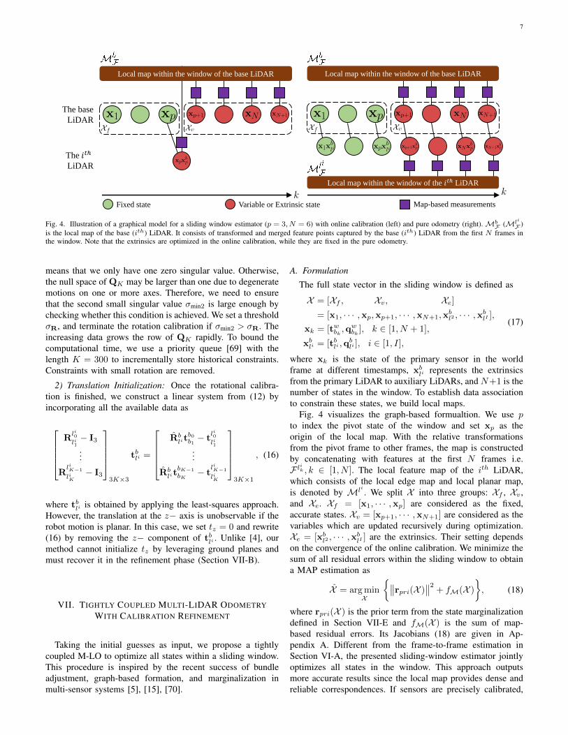
Fig. 4. Illustration of a graphical model for a sliding window estimator (p = 3, N = 6) with online calibration (left) and pure odometry (right).MbF (Mli

F )is the local map of the base (ith) LiDAR. It consists of transformed and merged feature points captured by the base (ith) LiDAR from the first N frames inthe window. Note that the extrinsics are optimized in the online calibration, while they are fixed in the pure odometry.

means that we only have one zero singular value. Otherwise,the null space of QK may be larger than one due to degeneratemotions on one or more axes. Therefore, we need to ensurethat the second small singular value σmin2 is large enough bychecking whether this condition is achieved. We set a thresholdσR, and terminate the rotation calibration if σmin2 > σR. Theincreasing data grows the row of QK rapidly. To bound thecomputational time, we use a priority queue [69] with thelength K = 300 to incrementally store historical constraints.Constraints with small rotation are removed.

2) Translation Initialization: Once the rotational calibra-tion is finished, we construct a linear system from (12) byincorporating all the available data as

Rli0li1− I3...

RliK−1

liK− I3

3K×3

tbli =

Rblit

b0b1− t

li0li1

...

Rblit

bK−1

bK− t

liK−1

liK

3K×1

, (16)

where tbli is obtained by applying the least-squares approach.However, the translation at the z− axis is unobservable if therobot motion is planar. In this case, we set tz = 0 and rewrite(16) by removing the z− component of tbli . Unlike [4], ourmethod cannot initialize tz by leveraging ground planes andmust recover it in the refinement phase (Section VII-B).

VII. TIGHTLY COUPLED MULTI-LIDAR ODOMETRYWITH CALIBRATION REFINEMENT

Taking the initial guesses as input, we propose a tightlycoupled M-LO to optimize all states within a sliding window.This procedure is inspired by the recent success of bundleadjustment, graph-based formation, and marginalization inmulti-sensor systems [5], [15], [70].

A. Formulation

The full state vector in the sliding window is defined as

X = [Xf , Xv, Xe]= [x1, · · · ,xp,xp+1, · · · ,xN+1,x

bl2 , · · · ,xblI ],

xk = [twbk ,qwbk

], k ∈ [1, N + 1],

xbli = [tbli ,qbli ], i ∈ [1, I],

(17)

where xk is the state of the primary sensor in the worldframe at different timestamps, xbli represents the extrinsicsfrom the primary LiDAR to auxiliary LiDARs, and N+1 is thenumber of states in the window. To establish data associationto constrain these states, we build local maps.

Fig. 4 visualizes the graph-based formualtion. We use pto index the pivot state of the window and set xp as theorigin of the local map. With the relative transformationsfrom the pivot frame to other frames, the map is constructedby concatenating with features at the first N frames i.e.F lik , k ∈ [1, N ]. The local feature map of the ith LiDAR,which consists of the local edge map and local planar map,is denoted by Mli . We split X into three groups: Xf , Xv ,and Xe. Xf = [x1, · · · ,xp] are considered as the fixed,accurate states. Xv = [xp+1, · · · ,xN+1] are considered as thevariables which are updated recursively during optimization.Xe = [xbl2 , · · · ,xblI ] are the extrinsics. Their setting dependson the convergence of the online calibration. We minimize thesum of all residual errors within the sliding window to obtaina MAP estimation as

X = arg minX

{∥∥rpri(X )∥∥2 + fM(X )

}, (18)

where rpri(X ) is the prior term from the state marginalizationdefined in Section VII-E and fM(X ) is the sum of map-based residual errors. Its Jacobians (18) are given in Ap-pendix A. Different from the frame-to-frame estimation inSection VI-A, the presented sliding-window estimator jointlyoptimizes all states in the window. This approach outputsmore accurate results since the local map provides dense andreliable correspondences. If sensors are precisely calibrated,

8

the constraints from other LiDARs are also used. According tothe convergence of calibration, we divide the problem into twosubtasks: online calibration (variable Xe) and pure odometry(fixed Xe). At each task, the definition of fM(X ) is different,and we present the details in Section VII-B and VII-C.

B. Optimization With Online CalibrationWe exploit the map-based measurements to refine the coarse

initialization results. Here, we treat the calibration as a reg-istration problem. fM(X ) is divided into two functions w.r.t.Xv and Xe. For states in Xv , the constraints are constructedfrom correspondences between features of the primary sensorat the latest frames i.e. Fbk , k ∈ [p+1, N+1] and those of theprimary local map i.e.Mb. For states in Xe, the constraints arebuilt up from correspondences between features of auxiliaryLiDARs at the pth frame i.e. F l

ip and the map Mb.

The correspondences between Fbk andMb are found usingthe method in [16]. KD-Tree is used for fast indexing in a map.1) For each edge point, we find a set of its nearest points in thelocal edge map within a specific region. This set is denotedby S, and its covariance is then computed. The eigenvectorassociated with the largest value implies the direction of thecorresponding edge line. By calculating the mean of S, theposition of this line is also determined. 2) For each planarpoint, the coefficients of the corresponding plane in the localplanar map are obtained by solving a linear system such asws + d = 0,∀s ∈ S. Similarly, we find correspondencesbetween F l

ip and Mb. Finally, we define the objective as the

sum of all measurement residuals for the online calibration asfM(X ) = fM(Xv) + fM(Xe)

=

N+1∑k=p+1

∑p∈Fbk

ρ(∥∥rF (x−1p xk,p)

∥∥2Σp

)

+

I∑i=2

∑p∈Flip

ρ(∥∥rF (xbli ,p)

∥∥2Σp

),

(19)

where x−1p xk defines the relative transformation from the pivotframe to the kth frame.

C. Optimization With Pure OdometryOnce we finish the online calibration by fulfilling the

convergence criterion (Section VII-D), the optimization withpure odometry given accurate extrinsics is then performed.In this case, we do not optimize the extrinsics, and utilizeall available map-based measurement to improve the single-LiDAR odometry. We incorporate constraints between featuresof all LiDARs and local maps into the cost function as

fM(X ) = fM(Xv)

=N+1∑k=p+1

∑p∈Fbk

ρ(∥∥rF (x−1p xk,p)

∥∥2Σp

)

+

I∑i=2

N+1∑k=p+1

∑p∈Fli

k

ρ(∥∥rF (x−1p xkx

bli ,p)

∥∥2Σp

),

(20)

where x−1p xkxbli is the transformation from the primary Li-

DAR at the pivot frame to auxiliary LiDARs at the kth frame.

Algorithm 1: Monitoring Calibration Convergence

Input: objective fM(·), current extrinsics x , xbliOutput: optimal extrinsics x, covariance matrix Ξcalib

1 Denote L the set of all eligible estimates;2 if calibration is ongoing then3 Linearize fM at x to obtain Λ = (∂fM∂x )> ∂fM∂x ;4 Compute the smallest eigenvalue λ of Λ;5 if λ > λcalib then6 Set x as the current extrinsics of the system;7 L ← L ∪ x;8 if |L| > Lcalib then9 x← E[x] as the mean;

10 Ξcalib ← Cov[x] as the covariance;11 Stop the online calibration;

12 return x, Ξcalib

D. Monitoring the Convergence of CalibrationWhile working on the online calibration in an unsupervised

way, it is of interest to decide whether calibration converges.After the convergence, we fix the extrinsics. This is beneficialto our system since both the odometry and mapping aregiven more geometric constraints from auxiliary LiDARs formore accurate poses. As derived in [34], the degeneracyfactor λ, which is the smallest eigenvalue of the informationmatrix, reveals the condition of an optimization-based stateestimation problem. Motivated by this work, we use λ toindicate whether our problem contains sufficient constraintsor not for accurate extrinsics. The detailed pipeline to updateextrinsics and monitor the convergence is summarized inAlgorithm 1. The algorithm takes the function fM(·) definedin (19) as well as the current extrinsics as input, and returnsthe optimized extrinsics. On line 4, we compute λ from theinformation matrix of the cost function. On lines 5–7, theextrinsics are updated if λ is larger than a threshold. Online 8, we use the number of candidate extrinsics to checkthe convergence. On lines 9–10, the convergence criterion ismet, and the termination is thus triggered. We then computethe sampling mean of L as the resulting extrinsics and thesampling covariance as the calibration covariance.

E. MarginalizationWe apply the marginalization technique to remove the oldest

variable states in the sliding window. The marginalizationis a process to incorporates historical constraints as a priorinto the objective, which is an essential step to maintain theconsistency of odometry and calibration results. In our system,xp is the only state to be marginalized after each optimization.By applying the Schur complement, we obtain the linear infor-mation matrix Λ∗rr and residual g∗r w.r.t. the remaining states.The prior residuals are formulated as ‖rpri‖2 = g∗>r Λ∗−1rr g∗r .Appendix B provides some mathematical foundations.

VIII. UNCERTAINTY-AWARE MULTI-LIDAR MAPPING

We first review the pipeline of the mapping module oftypical LiDAR SLAM systems [16]–[18]. Taking the prior

9

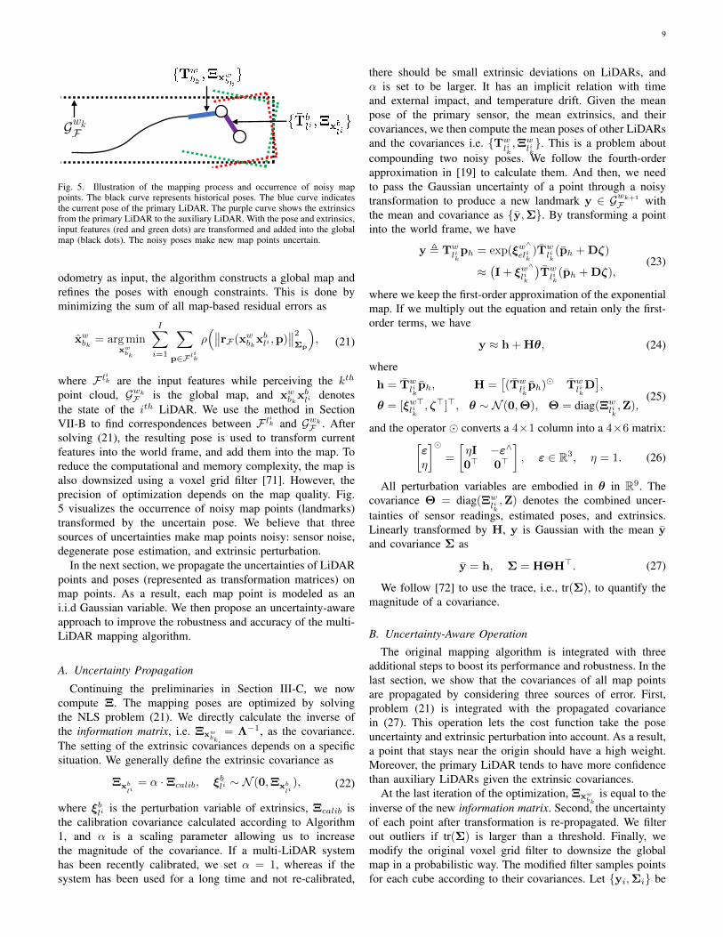
Fig. 5. Illustration of the mapping process and occurrence of noisy mappoints. The black curve represents historical poses. The blue curve indicatesthe current pose of the primary LiDAR. The purple curve shows the extrinsicsfrom the primary LiDAR to the auxiliary LiDAR. With the pose and extrinsics,input features (red and green dots) are transformed and added into the globalmap (black dots). The noisy poses make new map points uncertain.

odometry as input, the algorithm constructs a global map andrefines the poses with enough constraints. This is done byminimizing the sum of all map-based residual errors as

xwbk = arg minxwbk

I∑i=1

∑p∈Fli

k

ρ(∥∥rF (xwbkxbli ,p)

∥∥2Σp

), (21)

where F lik are the input features while perceiving the kth

point cloud, Gwk

F is the global map, and xwbkxbli denotesthe state of the ith LiDAR. We use the method in SectionVII-B to find correspondences between F lik and Gwk

F . Aftersolving (21), the resulting pose is used to transform currentfeatures into the world frame, and add them into the map. Toreduce the computational and memory complexity, the map isalso downsized using a voxel grid filter [71]. However, theprecision of optimization depends on the map quality. Fig.5 visualizes the occurrence of noisy map points (landmarks)transformed by the uncertain pose. We believe that threesources of uncertainties make map points noisy: sensor noise,degenerate pose estimation, and extrinsic perturbation.

In the next section, we propagate the uncertainties of LiDARpoints and poses (represented as transformation matrices) onmap points. As a result, each map point is modeled as ani.i.d Gaussian variable. We then propose an uncertainty-awareapproach to improve the robustness and accuracy of the multi-LiDAR mapping algorithm.

A. Uncertainty Propagation

Continuing the preliminaries in Section III-C, we nowcompute Ξ. The mapping poses are optimized by solvingthe NLS problem (21). We directly calculate the inverse ofthe information matrix, i.e. Ξxw

bk= Λ−1, as the covariance.

The setting of the extrinsic covariances depends on a specificsituation. We generally define the extrinsic covariance as

Ξxbli

= α ·Ξcalib, ξbli ∼ N (0,Ξxbli

), (22)

where ξbli is the perturbation variable of extrinsics, Ξcalib isthe calibration covariance calculated according to Algorithm1, and α is a scaling parameter allowing us to increasethe magnitude of the covariance. If a multi-LiDAR systemhas been recently calibrated, we set α = 1, whereas if thesystem has been used for a long time and not re-calibrated,

there should be small extrinsic deviations on LiDARs, andα is set to be larger. It has an implicit relation with timeand external impact, and temperature drift. Given the meanpose of the primary sensor, the mean extrinsics, and theircovariances, we then compute the mean poses of other LiDARsand the covariances i.e. {Tw

lik,Ξw

lik}. This is a problem about

compounding two noisy poses. We follow the fourth-orderapproximation in [19] to calculate them. And then, we needto pass the Gaussian uncertainty of a point through a noisytransformation to produce a new landmark y ∈ Gwk+1

F withthe mean and covariance as {y,Σ}. By transforming a pointinto the world frame, we have

y , Twlik

ph = exp(ξw∧

elik)Tw

lik(ph + Dζ)

≈(I + ξw

∧

lik

)Twlik

(ph + Dζ),(23)

where we keep the first-order approximation of the exponentialmap. If we multiply out the equation and retain only the first-order terms, we have

y ≈ h + Hθ, (24)

where

h = Twlik

ph, H =[(Tw

likph)� Tw

likD],

θ = [ξw>lik, ζ>]>, θ ∼ N (0,Θ), Θ = diag(Ξw

lik,Z),

(25)

and the operator � converts a 4×1 column into a 4×6 matrix:[εη

]�=

[ηI −ε∧0> 0>

], ε ∈ R3, η = 1. (26)

All perturbation variables are embodied in θ in R9. Thecovariance Θ = diag(Ξw

lik,Z) denotes the combined uncer-

tainties of sensor readings, estimated poses, and extrinsics.Linearly transformed by H, y is Gaussian with the mean yand covariance Σ as

y = h, Σ = HΘH>. (27)

We follow [72] to use the trace, i.e., tr(Σ), to quantify themagnitude of a covariance.

B. Uncertainty-Aware Operation

The original mapping algorithm is integrated with threeadditional steps to boost its performance and robustness. In thelast section, we show that the covariances of all map pointsare propagated by considering three sources of error. First,problem (21) is integrated with the propagated covariancein (27). This operation lets the cost function take the poseuncertainty and extrinsic perturbation into account. As a result,a point that stays near the origin should have a high weight.Moreover, the primary LiDAR tends to have more confidencethan auxiliary LiDARs given the extrinsic covariances.

At the last iteration of the optimization, Ξxwbk

is equal to theinverse of the new information matrix. Second, the uncertaintyof each point after transformation is re-propagated. We filterout outliers if tr(Σ) is larger than a threshold. Finally, wemodify the original voxel grid filter to downsize the globalmap in a probabilistic way. The modified filter samples pointsfor each cube according to their covariances. Let {yi,Σi} be

10

Screen

Camera

30°30°

0.75m

0.4m

Left LiDARRight LiDAR

(a) The Real handheld device. (b) Calibrated point cloud.

Fig. 6. (a) The real handheld device for indoor tests. Two VLP-16s aremounted at the left and right sides respectively. The attached camera is usedto record test scenes. (b) The calibrated point cloud consists of points fromthe left (red) and right (pink) LiDARs.

Top LiDAR

Left LiDAR

Right LiDAR

Front LiDAR

1.65m

(a) The Real vehicle. (b) Calibrated point cloud.

Fig. 7. (a) The real vehicle for large-scale, outdoor tests. Four RS-16sare mounted at the top, front, left, and right position respectively. (b) Thecalibrated point cloud consists of points from the top (red), front (green), left(blue), and right (pink) LiDARs.

the ith point in a cube, and M be the number of points in thecube. The sampled mean and covariance of a cube are

y =

M∑i=1

wiyi, Σ =

M∑i=1

w2iΣi, (28)

where w is the threshold, and wi = w−tr(Σi)∑mi=1[w−tr(Σi)]

is anormalized weight.

IX. EXPERIMENT

We perform simulated and real-world experiments on threeplatforms to test the performance of M-LOAM. First, wecalibrate multi-LiDAR systems on all the presented platforms.The proposed algorithm is compared with SOTA methods, andtwo evaluation metrics are introduced. Second, we demonstratethe SLAM performance of M-LOAM in various scenarioscovering indoor environments and outdoor urban roads. More-over, to evaluate the sensibility of M-LOAM against extrinsicerror, we test it on the handheld device and vehicle underdifferent levels of extrinsic perturbation. Finally, we providea study to comprehensively evaluate M-LOAM’s performanceand computation time with different LiDAR combinations.

A. Implementation Details

We use the PCL library [71] to process point clouds and theCeres Solver [73] to solve nonlinear least-squares problems.In experiments which are not specified, our algorithm isexecuted on a desktop with an i7 CPU@4.20 GHz and 32 GBRAM. Three platforms with different multi-LiDAR systemsare tested: a simulated robot, a handheld device, and a vehicle.

TABLE IIPARAMETERS FOR CALIBRATION AND SLAM.

σR λcalib Lcalib N p w α

0.25 70 25 4 2 100 ≥ 1

The LiDARs on real platforms are synchronized with theexternal GPS clock triggered at an ns-level accuracy.• The Simulated Robot (SR) is built on the Gazebo [74].

Two 16-beam LiDARs are mounted on a mobile robot fortesting. We build a closed simulated rectangular room. Weuse the approach from [75] to set the LiDAR configura-tion for maximizing the sensing coverage. We moved therobot in the room at an average speed of 0.5m/s. Theground-truth extrinsics and poses are provided.

• The Real Handheld Device (RHD) is made for handheldtests and shown in Fig. 6. Its configuration is similar tothat of the SR. Besides two VLP-16s4, we also installa mini computer (Intel NUC) for data collection anda camera (mvBlueFOX-MLC200w) for recording testscenes. We used this device to collect data on the campuswith an average speed of 2m/s.

• The Real Vehicle (RV) is a vehicle for autonomous logis-tic transportation [11]. We conduct experiments on thisplatform to demonstrate that our system also performswell in large-scale, challenging outdoor environments.As shown in Fig. 7, four RS-LiDAR-16s5 are rigidlymounted at the top, front, left, and right positions respec-tively. We drove the vehicle through urban roads at anaverage speed of 3m/s. Ground-truth poses are obtainedfrom a coupled LiDAR-GPS-encoder localization systemthat was proposed in [48], [76].

Table II shows the parameters which are empirically set. σR,λcalib, and Lcalib are the convergence thresholds in calibration.Setting the last two parameters requires a preliminary trainingprocess, which is detailed in the supplementary material [77].p and N are the size of the local map and the sliding windowin the odometry respectively. w is the threshold of filteringuncertain points in mapping, and α is the scale of the extrinsiccovariance. We set α = 10 for the case of injecting largeperturbation in Section IX-D. Otherwise, α = 1.

B. Performance of Calibration

1) Evaluation Metrics: We introduce two metrics to assessthe LiDAR calibration results from different aspects:• Error Compared With Ground truth (EGT) computes

the distance between the ground truth and the estimatedvalues in terms of rotation and translation as

EGTR =∥∥ ln(RgtR

−1est)∨∥∥,

EGTt =∥∥tgt − test

∥∥, (29)

• Mean Map Entropy (MME) is proposed to measure thecompactness of a point cloud [78]. It has been exploredas a standard metric to assess the quality of registration if

4https://velodynelidar.com/products/puck5https://www.robosense.ai/rslidar/rs-lidar-16

11

TABLE IIICALIBRATED EXTRINSICS. ↓ INDICATES THAT THE LOWER THE VALUE, THE BETTER THE SCORE.

Case MethodRotation [deg] Translation [m]

EGTR [deg, ↓] EGTt [m, ↓] MME [↓]x y z x y z r = 0.3m r = 0.4m

SR1

(Lef

t-R

ight

) Auto-Calib 6.134 1.669 0.767 0.001 −0.635 −0.083 33.911 0.209 −2.016 −2.463

Proposed (Ini.) 44.154 7.062 1.024 −0.027 −0.719 0.000 8.229 0.328 −2.240 −2.685

Proposed (Ini.+Ref.) 40.870 0.397 0.237 −0.012 −0.475 −0.206 0.997 0.018 −2.690 −3.073

PS-Calib 40.021 −0.005 −0.010 0.001 −0.476 −0.218 0.037 0.003 −2.730 −3.115

W/O Calib 0.000 0.000 0.000 0.000 0.000 0.000 40.000 0.525 −2.358 −2.704

GT 40.000 0.000 0.000 0.000 −0.477 −0.220 − − −2.733 −3.111

SR2

(Lef

t-R

ight

) Auto-Calib 4.680 −1.563 0.647 0.032 −0.751 −0.022 35.337 0.339 −2.336 −2.447

Proposed (Ini.) 40.854 3.517 0.285 −0.019 −0.667 0.000 3.632 0.291 −2.607 −2.804

Proposed (Ini.+Ref.) 38.442 0.111 −0.037 0.000 −0.504 −0.205 1.549 0.030 −3.016 −3.192

PS-Calib 40.021 −0.005 −0.010 0.001 −0.476 −0.218 0.0365 0.003 −3.113 −3.306

W/O Calib 0.000 0.000 0.000 0.000 0.000 0.000 40.000 0.525 −2.875 −2.878

GT 40.000 0.000 0.000 0.000 −0.477 −0.220 − − −3.117 −3.313

RH

D(L

eft-

Rig

ht) Auto-Calib 7.183 −3.735 33.329 0.653 −2.006 −0.400 44.312 1.612 −3.612 −2.711

Proposed (Ini.) 36.300 0.069 −3.999 0.113 −0.472 −0.103 6.443 0.112 −3.664 −2.839

Proposed (Ini.+Ref.) 37.545 −0.376 0.773 0.066 −0.494 −0.113 2.491 0.064 −3.681 −2.862

CAD Model 40.000 0.000 0.000 0.000 −0.456 −0.122 2.077 0.092 −3.662 −2.833

W/O Calib 0.000 0.000 0.000 0.000 0.000 0.000 40.000 0.560 −3.696 −2.868

PS-Calib 39.629 −1.664 1.193 0.033 −0.540 −0.142 − − −3.696 −2.868

RV(T

op-F

ront

) Auto-Calib −19.634 21.610 −3.481 −0.130 −0.282 −0.850 22.852 0.791 −2.705 −2.282

Proposed (Ini.) 1.320 7.264 3.011 −0.324 0.227 0.000 3.217 1.433 −2.721 −2.332

Proposed (Ini.+Ref.) −2.057 6.495 2.133 0.528 −0.036 −1.102 0.274 0.081 −2.885 −2.370

CAD Model 0.000 10.000 0.000 0.795 0.000 −1.364 4.505 0.351 −2.771 −2.312

W/O Calib 0.000 0.000 0.000 0.000 0.000 0.000 7.227 1.252 −2.785 −2.306

PS-Calib −1.817 6.629 2.134 0.536 0.039 −1.131 − − −2.902 −2.416

ground truth is unavailable [79]. Given a calibrated pointcloud, the normalized mean map entropy is

MME =1

m

m∑i=1

ln[

det(2πe ·Cpi)], (30)

where m is the size of the point cloud and Cpiis the

sampling covariance within a local radius r around pi.For each calibration case, we select 10 consecutive framesof point clouds that contain many planes and computetheir average MME values for evaluation.

Since the perfect ground truth is unknown in real-worldapplications, we use the results of “PS-Calib” [12] as the“relative ground truth” to compute the EGT. PS-Calib isa well-understood, target-based calibration approach, whichshould have similar or superior accuracy to our method [80].Another metric is the MME, which computes the score inan unsupervised way. It can be interpreted as an information-theoretic measure of the compactness of a point cloud.

2) Calibration Results: The multi-LiDAR systems of allthe presented platforms are calibrated by our methods. To ini-tialize the extrinsics, we manually move these platforms withsufficient rotations and translations. Table III reports the re-sulting extrinsics, where two simulated cases (same extrinsics,different motions) and two real-world cases are tested. Due tolimited space, we only demonstrate the calibration betweenthe top LiDAR and front LiDAR on the vehicle. Our method

2 4 6 8 10

Frame

-4.0

-3.5

-3.0

-2.5

-2.0

Mea

n M

ap E

ntr

op

y

Mean Map Entropy Over Frames of Point Clouds

r =0.3m

r =0.4m

Auto-Calib

Proposed (Ini.+Ref.)

PS-Calib

W/O Calib

Fig. 8. The MME values over 10 consecutive frames of point clouds whichare calibrated by different approaches on the RHD platform. The lower thevalue, the better the score for a method.

is denoted by “Proposed (Ini.+Ref.)”, which is comparedwith an offline multi-LiDAR calibration approach [4] (“Auto-Calib”). Although Auto-Calib follows a similar initialization-refinement procedure to obtain the extrinsics, it is differentfrom our algorithm in several aspects. For example, Auto-Calib only uses planar features in refinement. And it assumesthat LiDARs’ views should have large overlapping regions.The hand-eye-based initial (“Proposed (Ini.)”), uncalibrated(“W/O Calib”), CAD (“CAD model” for real platforms), andground-truth (“GT”) extrinsics are also provided for reference.

Our hand-eye-based method successfully initializes the ro-

12

0 100 200 300 400 500 600 700

0.0

20.0

40.0

R [

deg

]Process of Online Calibration

Phase 1

Section V-B

Phase 2

Section VI-B

Phase 3

Section VI-C

roll pitch yaw

0 100 200 300 400 500 600 700-1.0

-0.5

0.0

t [m

]

x y z

0 100 200 300 400 500 600 700

Frame

0.0

0.2

0.4

Sin

gu

lar

Val

ue

0.0

50.0

100.0

150.0

Fac

tor

Fig. 9. Detailed illustration of the whole calibration process, including theinitialization and optimization with online calibration on the RHD. Differentphases are separated by bold dashed lines. In Phase 1, the initial rotation andtranslation are estimated with the singular value-based exit criteria (SectionVI-B). In Phase 2, the nonlinear optimization-based calibration refinementprocess is performed. The convergence is determined by the degeneracy factor(Section VII-D). Phase 3 only optimizes the LiDAR odometry with fixedextrinsics. The black lines in the bottom plot indicate the setting thresholdsσR and λcalib, which are defined in Section VII-D.

-6

-4

-2

0

2

X [

m]

-14-12-10-8-6-4-20

Y [m]

Start Point

End Point

Fig. 10. Calibration trajectory of the sensor suite estimated by M-LO on theRHD. The dot and diamond indicate the start and end point respectively.

tation offset (< 9deg) for all cases, but fails to recover thetranslation offset (> 0.3m) on the SR and RV. Both the simu-lated robot and vehicle have to perform planar movement witha long distance for initialization, making the recovery of thex−, y− translation poor due to the drift of motion estimation.The planar movement also causes the z− translation to beunobservable. But we can move the RHD in 6-DoF and rapidlygather rich constraints. Its initialization results are thus good.Regarding the online refinement, our algorithm outperformsAuto-Calib and demonstrates comparable performance withPS-Calib in terms of the EGT (< 3deg and < 0.07m) andMME metrics. Based on these results, we conclude that theinitialization phase can provide coarse rotational estimates, andthe refinement for precise extrinsics is required.

We explicitly show the test on the RHD in detail. In Fig.8, we plot all MME values over different frames of calibratedpoint clouds, where the results are consistent with Table III.Whether r is set to 0.3m or 0.4m, our method always has abetter score than Auto-Calib. Fig. 9 illustrates the calibrationprocess, with the trajectory of the sensor suite shown in Fig.10. This process is divided into three sequential phases: Phase1 (extrinsic initialization, Section VI-B), Phase 2 (odometrywith extrinsic refinement, Section VII-B), and Phase 3 (pureodometry and mapping, Section VII-C).

0 5 10 15

-4

-2

0

2

4

Y[m

]

Trajectories of All Simulated Sequences

SR01 SR02 SR05

0 5 10 15

-4

-2

0

2

4

Estimated Trajectories against GT

M-LOAM Groundtruth

0 5 10 15

X[m]

-4

-2

0

2

4

Y[m

]

SR03 SR04

0 5 10 15

X[m]

-4

-2

0

2

4M-LOAM Groundtruth

Fig. 11. (Left) Trajectories of the SR01-SR05 sequences with different lengths.(Right) M-LOAM’s trajectories compared against the ground truth.

TABLE IVATE [81] ON SIMULATED SEQUENCES

Metric Sequence Length M-LOM-LOAM

-wo-uaM-LOAM A-LO A-LOAM

RM

SEt[m

] SR01easy 40.6m 0.482 0.041 0.041 2.504 0.060

SR02easy 39.1m 0.884 0.034 0.034 3.721 0.060

SR03hard 49.2m 0.838 0.032 0.032 4.738 0.059

SR04hard 74.2m 0.757 0.032 0.032 2.083 0.388

SR05hard 81.2m 0.598 0.033 0.033 4.841 0.208

RM

SER

[deg

] SR01easy 40.6m 3.368 0.824 0.676 26.484 0.751

SR02easy 39.1m 7.971 1.070 0.882 37.903 0.576

SR03hard 49.2m 6.431 0.994 0.865 38.923 0.750

SR04hard 74.2m 5.728 0.919 0.772 21.027 0.711

SR05hard 81.2m 6.509 0.754 0.554 87.999 2.250

Phase 1 starts with recovering the rotational offsets withoutprior knowledge about the mechanical configuration. It exitswhen the second small singular value of QK is larger thana threshold. The translational components are then computed.Phase 2 performs a nonlinear optimization to jointly refinethe extrinsics. This process may last for a prolonged periodif there are not sufficient environmental constraints. However,our sliding window-based marginalization scheme can ensurea bounded-complexity program to consistently update theextrinsics. The convergence condition is monitored with thedegeneracy factor (Section VII-D) and number of candidates.After convergence, we turn off the calibration and enter Phase3 that is evaluated in Section IX-C.

We also evaluate the sensitivity of our refinement methodto different levels of initial guesses: the CAD model as wellas rough rotational and translational initialization. Quantitativeresults can be found in the supplementary material [77].

C. Performance of SLAM

We evaluate M-LOAM on both simulated and real-worldsequences which are collected by the SR, RHD, and RVplatforms. The multi-LiDAR systems are calibrated with ouronline approach (Section VII-B). The detailed extrinsics canbe found on the first, third, and fourth row in Table III.

13

Fig. 12. Trajectories on SR05 of M-LOAM-wo-ua, M-LOAM, and A-LOAMand the map constructed by M-LOAM. A-LOAM has a few defects, whileM-LOAM-wo-ua’s trajectory nearly overlaps with that of M-LOAM.

8.0 16.0 24.0 32.0 40.0Distance Traveled [m]

0.01.53.04.56.07.5

Rot

atio

nE

rror

[deg

]

8.0 16.0 24.0 32.0 40.00.00.10.20.30.40.50.60.7

Tran

slat

ion

Err

or[m

] Relative Pose ErrorM-LOAM-wo-uaM-LOAMA-LOAM

Fig. 13. The mean RPE on SR05 with 10 trials. For the distance 40m, themedian values of the relative translation and rotation error of M-LOAM-wo-ua, M-LOAM, and A-LOAM are (0.87deg, 0.07m), (0.62deg, 0.06m), and(1.26deg, 0.22m) respectively.

We compare M-LOAM with two SOTA, open-source LiDAR-based algorithms: A-LOAM6 (the advanced implementation ofLOAM [16]) and LEGO-LOAM7 [17]. Both of them directlytake the calibrated and merged point clouds as input. Incontrast, our method formualtes the sliding-window estimatorto fuse point clouds. There are many differences in detailamong these methods, as presented in the technical sections.Overall, our system is more complete with online calibration,uncertainty estimation, and probabilistic mapping. LEGO-LOAM is a ground-optimized system and requires LiDARsto be horizontally installed. It easily fails on the SR andRV. We thus provide its results only on the RV sequencesfor a fair comparison. The results estimated by parts of M-LOAM are also provided. These are denoted by M-LO andM-LOAM-wo-ua, indicating our proposed odometry (SectionVII-C) and the complete M-LOAM without the awarenessof uncertainty (Section VIII-B), respectively. To fulfill thereal-time requirement, we run the odometry at 10Hz and themapping at 5Hz.

1) Simulated Experiment: We move the SR to follow5 paths with the same start point to verify our method.Each sequence is performed with 10-trial SLAM tests, andat each trial, zero-mean Gaussian noises with an SD of0.05m are added onto the point clouds. The ground-truth

6https://github.com/HKUST-Aerial-Robotics/A-LOAM7https://github.com/RobustFieldAutonomyLab/LeGO-LOAM

(a) Poses and the map with covariance visualization (b) Scene image

Fig. 14. (a) Side view of sample poses with covariances estimated by M-LOAM and generated map on RHD01corridor. The below blue map is createdby M-LOAM-wo-ua. The upper red map is created with M-LOAM. Thecovariances of pose calculated by M-LOAM are visualized as blue ellipses.A large radius represents a high uncertainty of a pose. The pose estimates inthe x–, z– direction are degenerate and uncertain, making the map points onthe ceiling and ground noisy. M-LOAM is able to maintain the map qualityby smoothing the noisy points. (b) The scene image.

(a) Map and trajectories (b) Trajectories

high

low

1

2

i

i

12

i

(c) Pose and map points with uncertainties

1

2(d) Scene images

Fig. 15. Results on RHD02lab. (a) Map generated in a laboratory andestimated trajectories (from right to left). The black box is the region shown inthe bottom figures. Two loops are in this sequence. (b) Trajectories in anotherviewpoint. (c) Visualization of poses and map points uncertainty. The grid sizeis 5m. Covariances of poses are represented as blue ellipses. The larger theradius, the higher the uncertainty. The uncertainty of a point is measured bythe trace of its covariance. The larger the trace, the higher the uncertainty. Themarked regions indicate the degenerate (scene 1) and well-conditioned (scene2) pose estimation respectively. With compounded uncertainty propagation,the map points in scene 1 become uncertain. (d) Scene images.

and the estimated trajectories of M-LOAM are plotted inFig. 11. The absolute trajectory error (ATE) on all sequencesis shown in Table IV, as evaluated in terms of root-mean-square error (RMSE) [81]. All sequences are split into eitheran easy or hard level according to their length. First, M-LO outperforms A-LO around 4 − 10 orders of magnitudes,which shows that the sliding-window estimator can refinethe frame-to-frame odometry. Second, we observe that the

14

(a) Map and M-LOAM’s trajectory. (b) Scene image.

Fig. 16. Results of RHD03garden. (a) Map generated in a garden, and thetrajectory estimated by M-LOAM. The colors of the points vary from blue tored, indicating the altitude changes (0m to 23m) (b) Scene images.

Fig. 17. Mapping results of RHD04building that goes through the HKUSTacademic buildings and the trajectories estimated by different methods (totallength is 700m). The map is aligned with Google Maps. The colors of thepoints vary from blue to red, indicating the altitude changes (0m to 40m)

mapping module greatly refines the odometry module. Third,M-LOAM outperforms other methods in most cases. This isdue to two main reasons. 1) The small calibration error maypotentially affect the map quality and degrade M-LOAM-wo-ua’s and A-LOAM’s performance. 2) The estimates from A-LO do not provide a good pose prior to A-LOAM. Sincethe robot has to turn around in the room for exploration, A-LOAM’s mapping error accumulates rapidly and thus makesthe optimized poses worse. This explains why A-LOAM haslarge error in SR04hard and SR05hard. One may argue thatA-LOAM has less rotational error than other methods onSR02easy – SR04hard. We explain that A-LOAM uses groundpoints to constrain the roll and pitch angles, while M-LOAMtends to filter them out.

We show the results of SR05hard in detail. The estimatedtrajectories are shown in Fig. 12. A-LOAM has a few defectsin the marked box region and at the tail of their trajectories,while M-LOAM-wo-ua’s trajectory nearly overlaps with thatof M-LOAM. The relative pose errors (RPE) evaluated by [81]are shown in Fig. 13. In this plot, M-LOAM has lower rotationand translation errors than others over a long distance.

2) Indoor Experiment: We used the handheld device tocollect four sequences called RHD01corridor, RHD02lab,

TABLE VMEAN RELATIVE POSE DRIFT

Sequence Length M-LOM-LOAM

-wo-uaM-LOAM A-LO A-LOAM

RHD02 197m 3.82% 0.29% 0.07% 14.18% 1.13%

RHD03 164m 0.88% 0.029% 0.044% 5.31% 0.32%

RHD04 695m 7.30% 0.007% 0.003% 34.02% 6.03%

RHD03garden, and RHD04building to test our approach.The first experiment is done in a long and narrow corridor.

As emphasized in [62], this is a typical poorly-constrained en-vironment. Here we show that the uncertainty-aware operationis beneficial to our system. In Fig. 14, we illustrate the sampleposes of M-LOAM and the generated map on RHD01corridor.These ellipses represent the size of the pose covariances. Alarge radius indicates that the pose in the x−, z− directionsof each mapping step is uncertain. This is mainly causedby the fact that only a small set of points scan the wallsand ceiling, which cannot provide enough constraints. Mappoints become uncertain due to noisy transformations. Theuncertainty-aware operation of M-LOAM is able to captureand discard uncertain points. This leads to a map with areasonaly good signal-to-noise ratio, which generally improvesthe precision of optimization. This is the reason why M-LOAM outperforms M-LOAM-wo-ua.

We conduct more experiments to demonstrate the perfor-mance of M-LOAM on other RHD sequences. For evaluation,these datasets contain at least a closed loop. Our results ofRHD02lab are shown in Fig. 15. This sequence contains twoloops in a lab region. Fig. 15(a) shows M-LOAM’s map,and Fig. 15(b) shows the trajectories estimated by differentmethods. Both M-LOAM-wo-ua and A-LOAM accumulatessignificant drift at the x–, y–, z– directions after two loops,while M-LOAM’s results are almost drift free. Fig. 15(c)shows the estimated poses and map points in the first loop. Thecovariances of the poses and points evaluated by M-LOAMare visible as ellipses and colored dots in the figure. Besidesthe corridor in scene 1, we also mark the well-conditionedenvironment in scene 2 for comparison. Fig. 15(d) shows thescene pictures. The results fit our previous explanation thatthe points in scene 1 are uncertain because of noisy poses. Incontrast, scene 2 has more constraints for estimating poses,making the map points certain.

Fig. 16 shows the results of RHD03garden. Since theinstallation of LiDARs on the RHD has a large roll angle,the areas over a 20m height are scanned. Another experimentis carried out in a longer sequence. This dataset lasts for 12minutes, and the total length is about 700m. The estimatedtrajectories and M-LOAM’s map are aligned with Google Mapin Fig. 17. Both M-LOAM-wo-ua and M-LOAM provide moreaccurate and consistent results than A-LOAM.

Finally, we evaluate the pose drift of methods with 10repeated trials on RHD02–RHD04. We employ the point-to-plane ICP [20] to measure the distance between the start andend point. This ground truth distance is used to compare withthat of the estimates, and the mean relative drift is listed in

15

Fig. 18. Mapping results of urban road and estimated trajectory against theground truth on the RV sequence (total length is 3.23km). The colors of thepoints vary from blue to red, indicating the altitude changes (−5m to 105m).

323.0 646.0 969.0 1292.0 1616.0Distance Traveled [m]

05

10152025

Rot

atio

nE

rror

[deg

]

323.0 646.0 969.0 1292.0 1616.00

5

10

15

20

Tran

slat

ion

Err

or[%

] Relative Pose ErrorM-LOAM-wo-uaM-LOAMA-LOAMLEGO-LOAM

Fig. 19. RPE on the RV sequence. For the 1616m distance, the median valuesof the relative translation (in percentage) and rotation error of M-LOAM-wo-ua, M-LOAM, A-LOAM, and LEGO-LOAM are (6.90deg, 1.87%), (6.45deg,2.14%), (15.36deg, 2.80%), (9.33deg, 2.23%) respectively.

Table V. Both M-LOAM-wo-ua and M-LOAM achieve a sim-ilar accuracy on RHD03 and RHD04 since the surroundingsof these sequences are almost well-conditioned. We concludethat the uncertainty-aware operation is not really necessaryin well-conditioned environments and well-calibrated sensors,but maximally reduces the negative effect of uncertainties.

3) Outdoor Experiment: The large-scale, outdoor sequencewas recorded with the RV platform (Fig. 7). This sequencecovers an area around 1100m in length and 450m in widthand has 110m in height changes. The total path length is about3.23km. The data lasts for 38 minutes, and contains the 10-Hz point clouds from fdour LiDARs and 25-Hz ground-truthposes. This experiment is very significant to test the stabilityand durability of M-LOAM.

M-LOAM’s trajectory against the ground truth and the builtmap is aligned with Google Map in Fig. 18. We present theRPE of M-LOAM, M-LOAM-wo-ua, A-LOAM, and LEGO-LOAM in Fig. 19. A-LOAM has the highest errors amongthem. Both M-LOAM-wo-ua and M-LOAM have competitiveresults with LEGO-LOAM. In addition, the outlier terms ofM-LOAM are fewer than other methods. We thus extend ourprevious findings that the uncertainty-aware mapping has thecapability to enhance the robustness of the system.

D. Sensitivity to Noisy Extrinsics

In this section, we evaluate the sensitivity of M-LOAM todifferent levels of extrinsic perturbation. On the RHD and RV

(a) Trajectories in a down view. (b) Trajectories in another view.

Fig. 20. Trajectories on RHD02lab with being injected by a large extrinsicperturbation. The detailed settings are shown in Table VI.

Fig. 21. Trajectories on 341m-length sequence (a part of the RV sequence)injected with a large extrinsic perturbation. The detailed settings are shownin Table VI.

platforms, we test our method by setting the extrinsics withdifferent levels of accuracy: CAD model, initialization, andperturbation injection. The experiment settings are listed inTable VI. The injected perturbation is the simulated shock onthe ground truth extrinsics with [10, 10, 10]deg in roll, pitch,and yaw and [0.1, 0.1, 0.1]m along the x−, y−, and z− axes.We use RHD02lab and a partial sequence on RV to compareM-LOAM with the baseline methods. It should be noted thatextrinsic calibration is turned off, and we only use the topand front LiDAR on the vehicle in experiments. The estimatedtrajectories under the largest perturbation are shown in Fig. 20and Fig. 21 for different platforms. These methods are markedwith ‘(inj)’. We calculate the ATE in Table VI. Here, M-LOAM’s trajectory on RHD02lab in Section IX-C2 is used tocompute the error. We observe that all methods’ performancedegrades along with the increasing extrinsic perturbation. Butboth M-LOAM-wo-ua and M-LOAM have smaller error. Inparticular, under the largest perturbation, M-LOAM is muchmore robust since it can track sensors’ poses.

E. Single LiDAR v.s. Multiple LiDARs

In this section, we explore the specific improvements in uti-lizing more LiDARs in M-LOAM. The RV platform has fourLiDARs. We use One-, Two-, Three-, Four-LiDAR to denotethe setups of l1, l1,2, l1,2,3, and l1,2,3,4 respectively (Fig. 7(a)).We also use x-Odom and x-Map to denote results provided bythe odometry and mapping using different setups, respectively.The tests are carried out on the complete RV sequence. We

16

TABLE VIATE GIVEN DIFFERENT EXTRINSICS FROM BAD TO GOOD: INJECT PERTURBATION, INITIALIZATION, AND CAD MODEL.

Case Extrinsic SourceRotation [deg] Translation [m] ATE: RMSEt[m] (RMSER[deg])

x y z x y z M-LOAM-wo-ua M-LOAM A-LOAM LEGO-LOAM

RHD(Left-Right)

Inject Perturbation 49.629 8.236 11.193 0.133 −0.440 −0.042 7.74(29.63) 0.88(8.10) 4.16(17.79) −Initialization 36.300 0.069 −3.999 0.113 −0.472 −0.103 0.90(6.46) 0.79(6.92) 1.11(6.44) −CAD Model 40.000 0.000 0.000 0.000 −0.456 −0.122 0.53(3.61) 0.20(2.43) 0.53(3.94) −

RV(Top-Front)

Inject Perturbation 8.183 16.629 12.134 0.636 0.139 −1.031 0.75(4.05) 0.56(3.33) 17.85(15.46) 1.06(6.01)

Initialization 1.320 7.264 3.011 −0.324 0.227 0.000 0.67(3.45) 0.60(3.23) 11.72(8.37) 0.90(4.06)

CAD Model 0.000 10.000 0.000 0.795 0.000 −1.364 0.48(2.29) 0.43(2.56) 12.95(5.40) 0.73(2.44)

323.0 646.0 969.0 1292.0 1616.0Distance Traveled [m]

020406080

100

Rot

atio

nE

rror

[deg

]

323.0 646.0 969.0 1292.0 1616.00

1020304050

Tran

slat

ion

Err

or[%

] Relative Pose Error (3m/s)

One-LiDAR-OdomOne-LiDAR-Map

Two-LiDAR-OdomTwo-LiDAR-Map

Three-LiDAR-OdomThree-LiDAR-Map

Four-LiDAR-OdomFour-LiDAR-Map

(a) RPE in the case of 3m/s. From one to four LiDARs, the median values ofthe rotation and translation error (in percentage) in odometry are: (56.53deg,20.19%), (54.53deg, 19.29%), (48.08deg, 17.57%), (42.96deg, 15.73%)respectively, while those in mapping are: (6.27deg, 2.35%), (6.26deg,2.16%), (6.77deg, 2.32%), (6.45deg, 2.14%) respectively.

323.0 646.0 969.0 1292.0 1616.0Distance Traveled [m]

01020304050

Rot

atio

nE

rror

[deg

]

323.0 646.0 969.0 1292.0 1616.005

1015202530

Tran

slat

ion

Err

or[%

] Relative Pose Error (9m/s)

One-LiDAR-OdomOne-LiDAR-Map

Two-LiDAR-OdomTwo-LiDAR-Map

Three-LiDAR-OdomThree-LiDAR-Map

Four-LiDAR-OdomFour-LiDAR-Map

(b) RPE in the case of 9m/s. From one to four LiDARs, the medianvalues of the rotation and translation error (in percentage) in odometry are:(29.38deg, 11.56%), (28.67deg, 11.00%), (24.60deg, 9.83%), (21.02deg,8.01%) respectively, while those in the mapping are: (6.86deg, 2.42%),(6.43deg, 2.19%), (7.04deg, 2.24%), (6.06deg, 2.11%) respectively.

Fig. 22. RPE of M-LOAM on the RV sequence with different numbers of LiDARs in two cases. Better visualization in the colored version.

TABLE VIIAVERAGE FEATURE NUMBER AND RUNNING TIME ON A DESKTOP OFM-LOAM ON THE RV SEQUENCE WITH DIFFERENT LIDAR SETUPS.

Setup One-LiDAR Two-LiDAR Three-LiDAR Four-LiDAR

Edge features 1061 1366 1604 1851

Planar features 4721 5881 7378 8631

Measurement [ms] 4.6± 0.4 4.8± 0.5 5.5± 0.7 6.0± 0.7

Odometry [ms] 27± 5 57± 7 69± 7 73± 9

Mapping [ms] 78± 11 91± 13 111± 16 126± 15

*Specifications: Intel i7 CPU@4.20 GHz and 32 GB RAM

first report statistics of the program in Table VII, includingthe average number of edge and planar features as well asaverage running time of measurement processing, optimizationwith pure odometry, and uncertainty-aware mapping. We seethat the odometry time increases with more LiDARs becausethe system needs to handle more geometric constraints. Thisphenomenon does not appear in measurement preprocessingsince we parallelize this module. The mapping time does notgrow linearly because we use the voxel grid filter to boundthe map’s complexity. We also provide the running time on anIntel NUC (i7 CPU@3.1GHz) in the supplementary material[77], where the results are consistent with Table VII.

To demonstrate that more features boost the system per-formance, we conduct experiments in two cases: driving at anormal speed and high speed. We use the original RV sequencein the first case. To simulate that the vehicle is moving faster inthe second case, we extract one frame from every three framesto construct a new dataset. We evaluate the odometry andmapping of these setups in Fig. 22. The errors of the odometrydecrease if more LiDARs are used. In the second case, themedian values of Four-LiDAR-Odom are smaller than thoseof One-LiDAR-Odom around 8deg relative rotation error and3.5% translation error. But this improvement in mapping issmall because the map already provides sufficient constraints.When the vehicle is moving at a higher speed, the global mapbecomes sparser. Consequently, the improvement of mappingon multiple LiDARs is noticeable. The boxplot of the Four-LiDAR setup has a smaller variance than others.

X. DISCUSSION

A. Main Advantages

We highlight that M-LOAM is a robust, reliable, andcomplete system to provide accurate calibration, odometry,and mapping results for different multi-LiDAR systems. Wecan extend M-LOAM to many types of LiDAR combinations,as shown in experiments. A typical application of M-LOAM

17

is autonomous driving, where the multi-LiDAR system isgradually becoming a standard setup on vehicles. As verifiedin the experiments, the usage of multiple LiDARs boosts theSLAM performance in both robustness and accuracy. For otherperception problems such as 3D object detection [67] andtracking [82], the multi-LiDAR systems are also beneficial.

As compared with the SOTA, M-LOAM introduces the slid-ing window-based tightly-coupled odometry to fuse multipleLiDARs and the uncertainty-aware mapping to maintain theglobally consistent map with good noise-singal ratio. Further-more, rather than operating calibrated and merged point cloudsdirectly, it processes the multi-LiDAR measurements in anseparate way. This design is advantageous in several aspects:1) programs (e.g., segmentation and feature extraction) can beeasily parallelized, 2) the LiDAR’s scan models can be used togenerate a range image without data loss, and 3) the extrinsicperturbation on the system can be formulated. We considerthat the above improvements enable M-LOAM to outperformA-LOAM on most sequences. Compared with LEGO-LOAM,which uses ground features, M-LOAM is more applicable todiverse applications. Nevertheless, integrating M-LOAM withthe ground-optimization pipeline of LEGO-LOAM for mobilerobots is encouraging.

The Gaussian distribution is our core hypothesis in model-ing data uncertainty. Based on it, we use a tractable methodto estimate covariances of poses (derived from informationmatrices) and extrinsics (given a sampling covariance after cal-ibration). Even though these covariances are approximate, asshown in experiments, e.g., Fig. 20, the proposed uncertainty-aware operation significantly improves the robustness of M-LOAM against degeneracy and extreme extrinsic perturbation.

B. Limitations

We recognize that the proposed calibration and SLAMmethods have limitations. First, the calibration process requiressome pre-set thresholds which are obtained from experiments.Its accuracy is not perfect for applications such as HD mapconstruction. In practice, the errors should be smaller than0.01m and 1deg. Otherwise, the calibration errors are pro-portionally propagated to the map and deteriorate the mapquality. This effect cannot be entirely eliminated even thoughthe extrinsic perturbation is modeled by our method.

Second, our system utilizes several point cloud registrationsin different phases to estimate states. As a typical non-convexproblem, registration requires a good initial transformation.But LiDARs only produce a low-frequency data stream, mak-ing this problem sometimes challenging. For example, when arobot moves and turns at a high frequency, our method barelytracks its poses. Also, we use the linear model to interpolatesensors’ poses, which cannot represent smooth or fast motionwell. In these cases, it would be better to use high-order curvessuch as B-spline for interpolation [83].

Finally, we extract the simple edge and planar points fromenvironments. However, these features present drawbacks inreal tests. For instance, they only provide constraints in theirperpendicular directions. In a long tunnel, where all planes aremostly parallel, M-LOAM may fail. Another example is that

such features do not have enough recognition power to enablerobust matching across frames with large viewpoint changes.As compared with surfel-based or visual features, they are lessuseful for tasks such as place recognition and relocalization.

XI. CONCLUSION AND FUTURE WORK

In this paper, we propose a complete and robust solution formulti-LiDAR extrinsic calibration and SLAM. This approachcontains several desirable features, including fast segmentationfor noise removal, motion and extrinsic initialization, onlineextrinsic calibration with convergence identification, a tightlycoupled M-LO, and uncertainty-aware multi-LiDAR mapping.We conduct extensive experiments covering scenarios fromindoor offices to outdoor urban roads for evaluation. Our ap-proach calibrates kinds of multi-LiDAR systems for differentplatforms. It yields accuracies centimeters in translation anddeci-degrees in rotation and is comparable to a SOTA target-based method. For SLAM, the proposed system typicallyreaches a localization accuracy below 40cm in medium-scale(> 150m) scenarios and of a few meters in the large-scaleurban roads (> 3.2km). For the benefit of the community, wemake our implementation open-source.

There are several directions for future research. Adding aloop-closure module into our system is desirable, which helpsto correct the accumulated drift and keep the global map [84].Another research direction concerns object-centric SLAM.Two challenges are recently growing in the community. Onthe one hand, the widely used low-level geometric features arenot representative and sensitive to viewpoint change. On theother hand, data sparsity and occlusion in LiDAR-based objectdetectors are the dominant bottlenecks. A possible solution tothem is to develop a SLAM approach which can use object-level features to optimize both ego-motion and motion ofdynamic objects. Trials on cameras or visual-inertial systemshave been proposed in [85]–[87], while works on LiDARsare rare. Finally, extending our approach on calibration anduncertainty modeling to sensors in various modalities, e.g.,IMUs [5], radars [9] and event-cameras [88], is promising.For instance, we can propagate the IMU noise model to predictpose uncertainties, or the proposed convergence criteria can beused for the extrinsic calibration of multi-modal sensors.

APPENDIX

A. Jacobians of ResidualsThe state vector is defined as x = [t,q]. We convert q into

a rotation matrix R by the Rodrigues formula [59]:

R = (q2w − q>xyzqxyz)I + 2qxyzq>xyz + 2qwq∧xyz, (31)

1) Jacobians of rH: The residuals in (8) are rewritten as

rH(x,p) =[w>(Rp + t) + d

]w

= diag(w)[w w w

]>(Rp + t) + dw

= W(Rp + t) + dw,

(32)

Using the left perturbation: R exp(δφ∧) ≈ R(I+δφ∧), theJacobians of the rotation and translation are calculated as

∂rH(x,p)

∂x= [

∂rH(x,p)

∂t,∂rH(x,p)

∂q],

= [W, −WRp∧, 03×1].

(33)

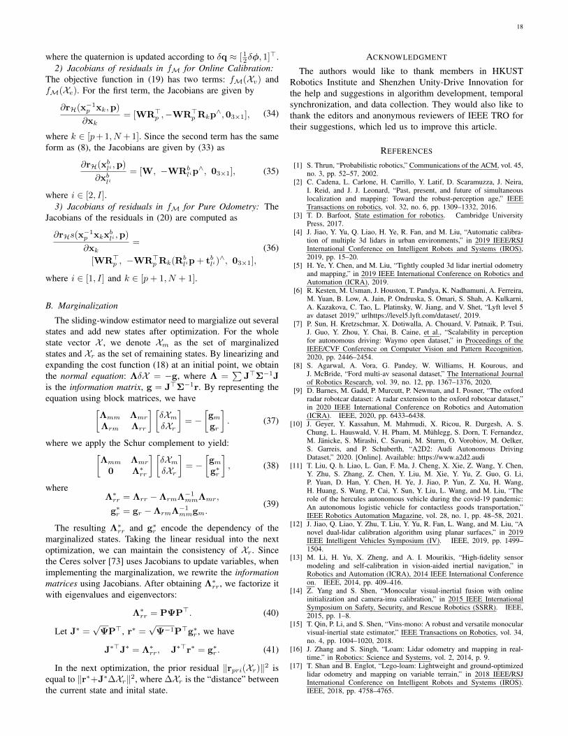
18

where the quaternion is updated according to δq ≈ [ 12δφ, 1]>.2) Jacobians of residuals in fM for Online Calibration:

The objective function in (19) has two terms: fM(Xv) andfM(Xe). For the first term, the Jacobians are given by

∂rH(x−1p xk,p)

∂xk= [WR>p ,−WR>p Rkp

∧,03×1], (34)

where k ∈ [p+ 1, N + 1]. Since the second term has the sameform as (8), the Jacobians are given by (33) as

∂rH(xbli ,p)

∂xbli= [W, −WRb

lip∧, 03×1], (35)

where i ∈ [2, I].3) Jacobians of residuals in fM for Pure Odometry: The

Jacobians of the residuals in (20) are computed as

∂rHs(x−1p xkx

bli ,p)

∂xk=

[WR>p , −WR>p Rk(Rblip + tbli)

∧, 03×1],

(36)

where i ∈ [1, I] and k ∈ [p+ 1, N + 1].

B. Marginalization

The sliding-window estimator need to margialize out severalstates and add new states after optimization. For the wholestate vector X , we denote Xm as the set of marginalizedstates and Xr as the set of remaining states. By linearizing andexpanding the cost function (18) at an initial point, we obtainthe normal equation: ΛδX = −g, where Λ =

∑J>Σ−1J

is the information matrix, g = J>Σ−1r. By representing theequation using block matrices, we have[

Λmm Λmr

Λrm Λrr

] [δXmδXr

]= −

[gmgr

]. (37)

where we apply the Schur complement to yield:[Λmm Λmr

0 Λ∗rr

] [δXmδXr

]= −

[gmg∗r

], (38)

whereΛ∗rr = Λrr −ΛrmΛ−1mmΛmr,

g∗r = gr −ΛrmΛ−1mmgm.(39)

The resulting Λ∗rr and g∗r encode the dependency of themarginalized states. Taking the linear residual into the nextoptimization, we can maintain the consistency of Xr. Sincethe Ceres solver [73] uses Jacobians to update variables, whenimplementing the marginalization, we rewrite the informationmatrices using Jacobians. After obtaining Λ∗rr, we factorize itwith eigenvalues and eigenvectors:

Λ∗rr = PΨP>. (40)

Let J∗ =√

ΨP>, r∗ =√

Ψ−1P>g∗r , we have

J∗>J∗ = Λ∗rr, J∗>r∗ = g∗r . (41)

In the next optimization, the prior residual ‖rpri(Xr)‖2 isequal to ‖r∗+J∗∆Xr‖2, where ∆Xr is the “distance” betweenthe current state and inital state.

ACKNOWLEDGMENT

The authors would like to thank members in HKUSTRobotics Institute and Shenzhen Unity-Drive Innovation forthe help and suggestions in algorithm development, temporalsynchronization, and data collection. They would also like tothank the editors and anonymous reviewers of IEEE TRO fortheir suggestions, which led us to improve this article.

REFERENCES

[1] S. Thrun, “Probabilistic robotics,” Communications of the ACM, vol. 45,no. 3, pp. 52–57, 2002.

[2] C. Cadena, L. Carlone, H. Carrillo, Y. Latif, D. Scaramuzza, J. Neira,I. Reid, and J. J. Leonard, “Past, present, and future of simultaneouslocalization and mapping: Toward the robust-perception age,” IEEETransactions on robotics, vol. 32, no. 6, pp. 1309–1332, 2016.

[3] T. D. Barfoot, State estimation for robotics. Cambridge UniversityPress, 2017.

[4] J. Jiao, Y. Yu, Q. Liao, H. Ye, R. Fan, and M. Liu, “Automatic calibra-tion of multiple 3d lidars in urban environments,” in 2019 IEEE/RSJInternational Conference on Intelligent Robots and Systems (IROS),2019, pp. 15–20.

[5] H. Ye, Y. Chen, and M. Liu, “Tightly coupled 3d lidar inertial odometryand mapping,” in 2019 IEEE International Conference on Robotics andAutomation (ICRA), 2019.

[6] R. Kesten, M. Usman, J. Houston, T. Pandya, K. Nadhamuni, A. Ferreira,M. Yuan, B. Low, A. Jain, P. Ondruska, S. Omari, S. Shah, A. Kulkarni,A. Kazakova, C. Tao, L. Platinsky, W. Jiang, and V. Shet, “Lyft level 5av dataset 2019,” urlhttps://level5.lyft.com/dataset/, 2019.

[7] P. Sun, H. Kretzschmar, X. Dotiwalla, A. Chouard, V. Patnaik, P. Tsui,J. Guo, Y. Zhou, Y. Chai, B. Caine, et al., “Scalability in perceptionfor autonomous driving: Waymo open dataset,” in Proceedings of theIEEE/CVF Conference on Computer Vision and Pattern Recognition,2020, pp. 2446–2454.

[8] S. Agarwal, A. Vora, G. Pandey, W. Williams, H. Kourous, andJ. McBride, “Ford multi-av seasonal dataset,” The International Journalof Robotics Research, vol. 39, no. 12, pp. 1367–1376, 2020.

[9] D. Barnes, M. Gadd, P. Murcutt, P. Newman, and I. Posner, “The oxfordradar robotcar dataset: A radar extension to the oxford robotcar dataset,”in 2020 IEEE International Conference on Robotics and Automation(ICRA). IEEE, 2020, pp. 6433–6438.

[10] J. Geyer, Y. Kassahun, M. Mahmudi, X. Ricou, R. Durgesh, A. S.Chung, L. Hauswald, V. H. Pham, M. Muhlegg, S. Dorn, T. Fernandez,M. Janicke, S. Mirashi, C. Savani, M. Sturm, O. Vorobiov, M. Oelker,S. Garreis, and P. Schuberth, “A2D2: Audi Autonomous DrivingDataset,” 2020. [Online]. Available: https://www.a2d2.audi

[11] T. Liu, Q. h. Liao, L. Gan, F. Ma, J. Cheng, X. Xie, Z. Wang, Y. Chen,Y. Zhu, S. Zhang, Z. Chen, Y. Liu, M. Xie, Y. Yu, Z. Guo, G. Li,P. Yuan, D. Han, Y. Chen, H. Ye, J. Jiao, P. Yun, Z. Xu, H. Wang,H. Huang, S. Wang, P. Cai, Y. Sun, Y. Liu, L. Wang, and M. Liu, “Therole of the hercules autonomous vehicle during the covid-19 pandemic:An autonomous logistic vehicle for contactless goods transportation,”IEEE Robotics Automation Magazine, vol. 28, no. 1, pp. 48–58, 2021.

[12] J. Jiao, Q. Liao, Y. Zhu, T. Liu, Y. Yu, R. Fan, L. Wang, and M. Liu, “Anovel dual-lidar calibration algorithm using planar surfaces,” in 2019IEEE Intelligent Vehicles Symposium (IV). IEEE, 2019, pp. 1499–1504.

[13] M. Li, H. Yu, X. Zheng, and A. I. Mourikis, “High-fidelity sensormodeling and self-calibration in vision-aided inertial navigation,” inRobotics and Automation (ICRA), 2014 IEEE International Conferenceon. IEEE, 2014, pp. 409–416.

[14] Z. Yang and S. Shen, “Monocular visual-inertial fusion with onlineinitialization and camera-imu calibration,” in 2015 IEEE InternationalSymposium on Safety, Security, and Rescue Robotics (SSRR). IEEE,2015, pp. 1–8.

[15] T. Qin, P. Li, and S. Shen, “Vins-mono: A robust and versatile monocularvisual-inertial state estimator,” IEEE Transactions on Robotics, vol. 34,no. 4, pp. 1004–1020, 2018.

[16] J. Zhang and S. Singh, “Loam: Lidar odometry and mapping in real-time.” in Robotics: Science and Systems, vol. 2, 2014, p. 9.

[17] T. Shan and B. Englot, “Lego-loam: Lightweight and ground-optimizedlidar odometry and mapping on variable terrain,” in 2018 IEEE/RSJInternational Conference on Intelligent Robots and Systems (IROS).IEEE, 2018, pp. 4758–4765.

19

[18] J. Lin and F. Zhang, “Loam livox: A fast, robust, high-precision lidarodometry and mapping package for lidars of small fov,” in 2020 IEEEInternational Conference on Robotics and Automation (ICRA). IEEE,2020, pp. 3126–3131.

[19] T. D. Barfoot and P. T. Furgale, “Associating uncertainty with three-dimensional poses for use in estimation problems,” IEEE Transactionson Robotics, vol. 30, no. 3, pp. 679–693, 2014.

[20] F. Pomerleau, F. Colas, R. Siegwart, and S. Magnenat, “Comparing icpvariants on real-world data sets,” Autonomous Robots, vol. 34, no. 3,pp. 133–148, 2013.

[21] A. Segal, D. Haehnel, and S. Thrun, “Generalized-icp.” in Robotics:science and systems, vol. 2, no. 4, 2009, p. 435.

[22] J. Serafin and G. Grisetti, “Nicp: Dense normal based point cloudregistration,” in Intelligent Robots and Systems (IROS), 2015 IEEE/RSJInternational Conference on. IEEE, 2015, pp. 742–749.

[23] M. Magnusson, A. Lilienthal, and T. Duckett, “Scan registration forautonomous mining vehicles using 3d-ndt,” Journal of Field Robotics,vol. 24, no. 10, pp. 803–827, 2007.

[24] J. Behley and C. Stachniss, “Efficient surfel-based slam using 3d laserrange data in urban environments.” in Robotics: Science and Systems,2018.

[25] X. Chen, A. Milioto, E. Palazzolo, P. Giguere, J. Behley, and C. Stach-niss, “Suma++: Efficient lidar-based semantic slam,” in 2019 IEEE/RSJInternational Conference on Intelligent Robots and Systems (IROS).IEEE, 2019, pp. 4530–4537.

[26] W. S. Grant, R. C. Voorhies, and L. Itti, “Finding planes in lidarpoint clouds for real-time registration,” in 2013 IEEE/RSJ InternationalConference on Intelligent Robots and Systems. IEEE, 2013, pp. 4347–4354.

[27] M. Velas, M. Spanel, and A. Herout, “Collar line segments for fastodometry estimation from velodyne point clouds,” in 2016 IEEEInternational Conference on Robotics and Automation (ICRA). IEEE,2016, pp. 4486–4495.

[28] G. Pandey, S. Giri, and J. R. Mcbride, “Alignment of 3d pointclouds with a dominant ground plane,” in 2017 IEEE/RSJ InternationalConference on Intelligent Robots and Systems (IROS). IEEE, 2017,pp. 2143–2150.

[29] S. W. Chen, G. V. Nardari, E. S. Lee, C. Qu, X. Liu, R. A. F. Romero,and V. Kumar, “Sloam: Semantic lidar odometry and mapping for forestinventory,” IEEE Robotics and Automation Letters, vol. 5, no. 2, pp.612–619, 2020.

[30] K. Ji, H. Chen, H. Di, J. Gong, G. Xiong, J. Qi, and T. Yi, “Cpfg-slam:a robust simultaneous localization and mapping based on lidar in off-road environment,” in 2018 IEEE Intelligent Vehicles Symposium (IV).IEEE, 2018, pp. 650–655.

[31] J. Jiao, Y. Zhu, H. Ye, H. Huang, P. Yun, L. Jiang, L. Wang, and M. Liu,“Greedy-based feature selection for efficient lidar slam,” in 2021 IEEEInternational Conference on Robotics and Automation (ICRA). IEEE,2021.

[32] M. Bosse, R. Zlot, and P. Flick, “Zebedee: Design of a spring-mounted 3-d range sensor with application to mobile mapping,” IEEE Transactionson Robotics, vol. 28, no. 5, pp. 1104–1119, 2012.

[33] A. Pfrunder, P. V. Borges, A. R. Romero, G. Catt, and A. Elfes, “Real-time autonomous ground vehicle navigation in heterogeneous environ-ments using a 3d lidar,” in 2017 IEEE/RSJ International Conference onIntelligent Robots and Systems (IROS). IEEE, 2017, pp. 2601–2608.

[34] J. Zhang, M. Kaess, and S. Singh, “On degeneracy of optimization-basedstate estimation problems,” in 2016 IEEE International Conference onRobotics and Automation (ICRA). IEEE, 2016, pp. 809–816.

[35] A. Hinduja, B.-J. Ho, and M. Kaess, “Degeneracy-aware factors withapplications to underwater slam.” in 2019 IEEE/RSJ InternationalConference on Intelligent Robots and Systems (IROS), 2019, pp. 1293–1299.

[36] J. Zhang and S. Singh, “Enabling aggressive motion estimation at low-drift and accurate mapping in real-time,” in 2017 IEEE InternationalConference on Robotics and Automation (ICRA). IEEE, 2017, pp.5051–5058.

[37] W. Zhen and S. Scherer, “Estimating the localizability in tunnel-likeenvironments using lidar and uwb,” in 2019 International Conferenceon Robotics and Automation (ICRA). IEEE, 2019, pp. 4903–4908.

[38] Z. Rong and N. Michael, “Detection and prediction of near-term stateestimation degradation via online nonlinear observability analysis,” in2016 IEEE International Symposium on Safety, Security, and RescueRobotics (SSRR). IEEE, 2016, pp. 28–33.

[39] S. Lynen, M. W. Achtelik, S. Weiss, M. Chli, and R. Siegwart, “A robustand modular multi-sensor fusion approach applied to mav navigation,”

in 2013 IEEE/RSJ international conference on intelligent robots andsystems. IEEE, 2013, pp. 3923–3929.

[40] G. Wan, X. Yang, R. Cai, H. Li, Y. Zhou, H. Wang, and S. Song, “Robustand precise vehicle localization based on multi-sensor fusion in diversecity scenes,” in 2018 IEEE International Conference on Robotics andAutomation (ICRA). IEEE, 2018, pp. 4670–4677.

[41] S. Zhao, Z. Fang, H. Li, and S. Scherer, “A robust laser-inertial odometryand mapping method for large-scale highway environments,” in 2019IEEE/RSJ International Conference on Intelligent Robots and Systems(IROS). IEEE, 2019.

[42] X. Zuo, P. Geneva, Y. Yang, W. Lee, Y. Liu, and G. Huang, “Lic-fusion: Lidar-inertial-camera odometry,” in 2013 IEEE/RSJ internationalconference on intelligent robots and systems. IEEE, 2019.

[43] C. Qin, H. Ye, C. E. Pranata, J. Han, and M. Liu, “Lins: A lidar-ineritalstate estimator for robust and fast navigation,” 2020.

[44] G. Hemann, S. Singh, and M. Kaess, “Long-range gps-denied aerial in-ertial navigation with lidar localization,” in 2016 IEEE/RSJ InternationalConference on Intelligent Robots and Systems (IROS). IEEE, 2016,pp. 1659–1666.

[45] T. Lowe, S. Kim, and M. Cox, “Complementary perception for handheldslam,” IEEE Robotics and Automation Letters, vol. 3, no. 2, pp. 1104–1111, 2018.

[46] C. Le Gentil, T. Vidal-Calleja, and S. Huang, “In2lama: Inertial lidarlocalisation and mapping,” in 2019 International Conference on Roboticsand Automation (ICRA). IEEE, 2019, pp. 6388–6394.

[47] ——, “In2laama: Inertial lidar localization autocalibration and map-ping,” IEEE Transactions on Robotics, 2020.

[48] L. Zheng, Y. Zhu, B. Xue, M. Liu, and R. Fan, “Low-cost gps-aidedlidar state estimation and map building,” in 2019 IEEE InternationalConference on Imaging Systems and Techniques (IST). IEEE, 2019,pp. 1–6.

[49] M. He, H. Zhao, F. Davoine, J. Cui, and H. Zha, “Pairwise lidarcalibration using multi-type 3d geometric features in natural scene,” inIntelligent Robots and Systems (IROS), 2013 IEEE/RSJ InternationalConference on. IEEE, 2013, pp. 1828–1835.

[50] D.-G. Choi, Y. Bok, J.-S. Kim, and I. S. Kweon, “Extrinsic calibration of2-d lidars using two orthogonal planes,” IEEE Transactions on Robotics,vol. 32, no. 1, pp. 83–98, 2015.

[51] B. Xue, J. Jiao, Y. Zhu, L. Zhen, D. Han, M. Liu, and R. Fan, “Automaticcalibration of dual-lidars using two poles stickered with retro-reflectivetape,” in 2019 IEEE International Conference on Imaging Systems andTechniques (IST). IEEE, 2019, pp. 1–6.

[52] R. Kummerle, G. Grisetti, and W. Burgard, “Simultaneous calibration,localization, and mapping,” in 2011 IEEE/RSJ International Conferenceon Intelligent Robots and Systems. IEEE, 2011, pp. 3716–3721.

[53] A. Teichman, S. Miller, and S. Thrun, “Unsupervised intrinsic calibrationof depth sensors via slam.” in Robotics: Science and Systems, vol. 248,2013, p. 3.

[54] L. Heng, G. H. Lee, and M. Pollefeys, “Self-calibration and visual slamwith a multi-camera system on a micro aerial vehicle,” Autonomousrobots, vol. 39, no. 3, pp. 259–277, 2015.

[55] Z. Ouyang, L. Hu, Y. LU, Z. W. Wang, X. Peng, and L. Kneip, “Onlinecalibration of exterior orientations of a vehicle-mounted surround-viewcamera system,” in 2020 IEEE International Conference on Roboticsand Automation (ICRA). IEEE, 2020.

[56] T. Qin and S. Shen, “Online temporal calibration for monocularvisual-inertial systems,” in 2018 IEEE/RSJ International Conference onIntelligent Robots and Systems (IROS). IEEE, 2018, pp. 3662–3669.

[57] C. Le Gentil, T. Vidal-Calleja, and S. Huang, “3d lidar-imu calibrationbased on upsampled preintegrated measurements for motion distortioncorrection,” in 2018 IEEE International Conference on Robotics andAutomation (ICRA). IEEE, 2018, pp. 2149–2155.

[58] K. Qiu, T. Qin, J. Pan, S. Liu, and S. Shen, “Real-time temporal androtational calibration of heterogeneous sensors using motion correlationanalysis,” IEEE Transactions on Robotics, 2020.

[59] J. Sola, “Quaternion kinematics for the error-state kalman filter,” arXivpreprint arXiv:1711.02508, 2017.

[60] V. Ila, L. Polok, M. Solony, P. Smrz, and P. Zemcik, “Fast covariancerecovery in incremental nonlinear least-squares solvers,” in 2015 IEEEInternational Conference on Robotics and Automation (ICRA). IEEE,2015, pp. 4636–4643.

[61] M. Bosse, G. Agamennoni, I. Gilitschenski, et al., Robust estimationand applications in robotics. Now Publishers, 2016.

[62] A. Censi, “An accurate closed-form estimate of icp’s covariance,”in Proceedings 2007 IEEE international conference on robotics andautomation. IEEE, 2007, pp. 3167–3172.

20

[63] F. Pomerleau, A. Breitenmoser, M. Liu, F. Colas, and R. Siegwart,“Noise characterization of depth sensors for surface inspections,” in2012 2nd International Conference on Applied Robotics for the PowerIndustry (CARPI). IEEE, 2012, pp. 16–21.

[64] M. Brossard, S. Bonnabel, and A. Barrau, “A new approach to 3d icpcovariance estimation,” IEEE Robotics and Automation Letters, vol. 5,no. 2, pp. 744–751, 2020.

[65] D. Landry, F. Pomerleau, and P. Giguere, “Cello-3d: Estimating thecovariance of icp in the real world,” in 2019 International Conferenceon Robotics and Automation (ICRA). IEEE, 2019, pp. 8190–8196.

[66] W. Maddern, G. Pascoe, C. Linegar, and P. Newman, “1 year, 1000km: The oxford robotcar dataset,” The International Journal of RoboticsResearch, vol. 36, no. 1, pp. 3–15, 2017.

[67] J. Jiao, P. Yun, L. Tai, and M. Liu, “Mlod: Awareness of extrinsicperturbation in multi-lidar 3d object detection for autonomous driving,”in 2020 IEEE/RSJ International Conference on Intelligent Robots andSystems (IROS), 2020, pp. 10 556–10 563.

[68] I. Bogoslavskyi and C. Stachniss, “Fast range image-based segmentationof sparse 3d laser scans for online operation,” in 2016 IEEE/RSJInternational Conference on Intelligent Robots and Systems (IROS).IEEE, 2016, pp. 163–169.

[69] T. H. Cormen, C. E. Leiserson, R. L. Rivest, and C. Stein, Introductionto algorithms. MIT press, 2009.

[70] S. Leutenegger, P. Furgale, V. Rabaud, M. Chli, K. Konolige, andR. Siegwart, “Keyframe-based visual-inertial slam using nonlinear op-timization,” Proceedings of Robotis Science and Systems (RSS) 2013,2013.

[71] R. B. Rusu and S. Cousins, “3d is here: Point cloud library (pcl),” in2011 IEEE international conference on robotics and automation. IEEE,2011, pp. 1–4.

[72] Y. Kim and A. Kim, “On the uncertainty propagation: Why uncertaintyon lie groups preserves monotonicity?” in 2017 IEEE/RSJ InternationalConference on Intelligent Robots and Systems (IROS). IEEE, 2017,pp. 3425–3432.

[73] S. Agarwal, K. Mierle, and Others, “Ceres solver,” http://ceres-solver.org.

[74] N. Koenig and A. Howard, “Design and use paradigms for gazebo,an open-source multi-robot simulator,” in 2004 IEEE/RSJ InternationalConference on Intelligent Robots and Systems (IROS)(IEEE Cat. No.04CH37566), vol. 3. IEEE, 2004, pp. 2149–2154.

[75] S. Mou, Y. Chang, W. Wang, and D. Zhao, “An optimal lidar configu-ration approach for self-driving cars,” arXiv preprint arXiv:1805.07843,2018.

[76] Y. Zhu, B. Xue, L. Zheng, H. Huang, M. Liu, and R. Fan, “Real-time,environmentally-robust 3d lidar localization,” in 2019 IEEE InternationalConference on Imaging Systems and Techniques (IST). IEEE, 2019,pp. 1–6.

[77] J. Jiao, H. Ye, Y. Zhu, and M. Liu, “Supplementary materialto: Robust odometry and mapping for multi-lidar systems withonline extrinsic calibration,” Tech. Rep., 2020. [Online]. Available:https://ram-lab.com/file/site/m-loam/supp.pdf

[78] D. Droeschel, J. Stuckler, and S. Behnke, “Local multi-resolution rep-resentation for 6d motion estimation and mapping with a continuouslyrotating 3d laser scanner,” in 2014 IEEE International Conference onRobotics and Automation (ICRA). IEEE, 2014, pp. 5221–5226.

[79] J. Razlaw, D. Droeschel, D. Holz, and S. Behnke, “Evaluation ofregistration methods for sparse 3d laser scans,” in 2015 EuropeanConference on Mobile Robots (ECMR). IEEE, 2015, pp. 1–7.

[80] K. Huang and C. Stachniss, “On geometric models and their accuracyfor extrinsic sensor calibration,” in 2018 IEEE International Conferenceon Robotics and Automation (ICRA). IEEE, 2018, pp. 1–9.

[81] Z. Zhang and D. Scaramuzza, “A tutorial on quantitative trajectory eval-uation for visual (-inertial) odometry,” in 2018 IEEE/RSJ InternationalConference on Intelligent Robots and Systems (IROS). IEEE, 2018,pp. 7244–7251.

[82] S. Zhang, D. Wang, F. Ma, C. Qin, Z. Chen, and M. Liu, “Robustpedestrian tracking in crowd scenarios using an adaptive gmm-basedframework,” in 2020 IEEE/RSJ International Conference on IntelligentRobots and Systems (IROS), 2020, pp. 9992–9998.

[83] C. Park, P. Moghadam, J. Williams, S. Kim, S. Sridharan, and C. Fookes,“Elasticity meets continuous-time: Map-centric dense 3d lidar slam,”arXiv preprint arXiv:2008.02274, 2020.

[84] X. Chen, T. Labe, A. Milioto, T. Rohling, O. Vysotska, A. Haag,J. Behley, C. Stachniss, and F. Fraunhofer, “Overlapnet: Loop closingfor lidar-based slam,” in Proc. of Robotics: Science and Systems (RSS),2020.

[85] S. Yang and S. Scherer, “Cubeslam: Monocular 3-d object slam,” IEEETransactions on Robotics, vol. 35, no. 4, pp. 925–938, 2019.

[86] J. Zhang, M. Henein, R. Mahony, and V. Ila, “Vdo-slam: A visualdynamic object-aware slam system,” arXiv preprint arXiv:2005.11052,2020.

[87] T. Qin, T. Chen, Y. Chen, and Q. Su, “Avp-slam: Semantic visualmapping and localization for autonomous vehicles in the parking lot,”in 2020 IEEE/RSJ International Conference on Intelligent Robots andSystems (IROS), 2020, pp. 5939–5945.

[88] G. Gallego, T. Delbruck, G. M. Orchard, C. Bartolozzi, B. Taba,A. Censi, S. Leutenegger, A. Davison, J. Conradt, K. Daniilidis, andD. Scaramuzza, “Event-based vision: A survey,” IEEE Transactions onPattern Analysis and Machine Intelligence, pp. 1–1, 2020.