lidar imaging through the ocean surface - princeton universityrcarmona/download/image/mine1.pdf ·...

Lidar Imaging Through the Ocean Surface

Rene CARMONA∗, Frederic CEROU†‡ and Benjamin BLASCO§

Department of Operations Research & Financial Engineering,Princeton University, Princeton, NJ 08544

June 30, 2000

Abstract

This work is concerned with the detection and the identification of immersed ob-jects. Our efforts have been motivated by, and concentrated on, the specific problemof the LIDAR imagery of underwater mines. The difficulties of this problem are illus-trated by the experimental data used in this study.

We follow the standard approach which suggests to model the surface elevationas a random field. We combine the statistical analysis needed needed for the modelof the roughness of the surface of the ocean with the physics of image forming whichinclude focusing/defocusing, scattering and backscattering of the light beams, andfinally the sensor noise, into a large simulation program. The latter is used to pro-duce realistic images and video sequences of moored mines as seen from airborneplatforms, making possible the analysis of the statistics of the image degradationprocess.

1 Introduction

The detection and the removal of sea-mines are of great importance to the Navy. In recentyears, the clearance of sea-mines has also gained nationwide support and internationalattention due to its implications to marine life protection. Motivated by the identificationand detection of sea-mines, we propose a complete analysis of thedirect model whichexplains the distortion present in gated LIDAR images of immersed objects. We developsystematic simulation tools which take into account the many physical mechanisms in-volved in the degradation of the images as LIDAR beams propagate through the air and

∗Partially supported by ONR grant N00178-99-1-9003 and N00178-00-1-9001†Supported by ONR grant N00178-00-1-9001‡Permanent address: IRISA-INRIA, Project Sigma2, Campus de Beaulieu, 35042 Rennes cedex, France§Intern from Ecole Polytechnique, France

1

Transurface LIDAR Imaging 2

the water, and especially through the air-water interface. Our simulation methodologyis part of a more general approach to underwater imaging, which has been of particularinterest to researchers in fields such as marine science and military defense and we be-lieve that our results will be useful in both military and civil applications in rescue andrecovery.

In order to generate random samples for the time evolution of the ocean surface, weuse classical models from physical oceanography and standard tools for Monte Carlosimulations. The process taking the expected image (think for example of a large metallicsphere) into the images produced by the LIDAR imaging systems is highly nonlinear,and even in the best case scenarios (see for example Figure 1) very different from thestandard linear models of blurring and additive noise used in classical image restoration.This degradation process has an unpredictable component, which needs to be modeledstatistically: fortunately, the roughness of the ocean surface can naturally be modeled asthe realization of a homogeneous random field with statistics described in spectral terms.As expected, another difficulty comes from the fact that the images suffer from sensornoise, but unexpectedly, this source of distortion is not the main obstacle to a successfulanalysis. In this study we model this noise as a Poisson shot (quantum) noise. But besidesthe sensor noise, the main sources of distortion of the images are twofold: First, the strongspatial modulations caused by wave focusing and defocusing (in the present study, weconcentrate on the effects of the capillary waves, essentially ignoring the contribution ofthe gravity waves); Second, the clutter produced by the lack of contrast between the raysreflected by the target and the rays backscattered by the ocean medium. Understandingthe image degradation process is only the first part of our research program, and it is clearthat the difficult challenge remains: inverting this process. This is addressed in [4] wherewe report on our results on the detection of the mines of the ML(DC) data set.

The paper is organized as follow. The two data sets used in this study are introduced inthe next section. The following Section 3 is devoted to the simulation of random samplesof the surface elevation, while Section 4 is concerned with the actual simulation of raytracing image forming process. We describe the separate components in sequence: thelaser, the receiver, the light propagation at the air/water interface, the small angle diffusionapproximation and the propagation in the water, the backscattering and finally, the sensorshot noise. Experimental results are reported in Section 5 and the paper ends with a shortconclusion explaining some of the shortcomings of our system, and some directions offuture research.

Most of the images reproduced in this report are still frames from animations whichcan be found at the URLhttp://chelsea.princeton.edu/ rcarmona .


2 Description of the Data

This section is devoted to the discussion of the main features of the experimental data, asthey were made available to us.

A First Data Set

We first describe the data set, which was at the origin of this study. This first data set con-sists of images of a fake mine taken during an experiment near Panama City in the Gulfof Mexico. These images were taken with a CCD camera mounted on a crane approxi-mately50 ft above the ocean surface, the images being taken at angles with the verticalvarying from0deg to 60deg. For the purpose of this experiment, the proxy for the mine wasa metallic spherical object with radius6 in, and it was kept between1 to 10 m below thesurface. Figure 1 shows a couple of generic images from this experiment.

Figure 1: Two typical images from the first data set. The distortion phenomenon describedin the introduction is obvious: the spherical object is broken into bright patches.

The variety of images contained in this data set demonstrates the great sensitivity ofLIDAR returns to the magnitude of wave slopes as well as to the incident angle of thesensing rays. But it is fair to emphasize that the water was relatively calm during the twodays of the experiment.

A Second Data Set

The second data set is from the June 1995 ML(DC) Flight Verification Test conductedin the Gulf of Mexico, off the coast of Panama City. Figure 2 gives a typical exampleof the image files contained in this data set. Because of the pattern leading to the5thimage from the left, it is possible that a foreign object (possibly a mine) was present when


these images were collected. Unfortunately, direct information on the possible presenceof foreign objects in some of these images is not part of the package. In can only beinferred indirectly.

Figure 2: Image returns from 6 different gates (the depth of the gate increases when wego from the left to the right.)

The Magic Lantern Development Contingency (ML(DC)) system is a ranged-gatedlight detection and ranging (LIDAR) system, consisting of three main optical subsystems:the scanner, the laser and a set of six imaging receivers. The six imaging receivers arelocked on six overlapping gates, the depths of these gates being reported in Table 2 below.The images produced by the six receivers are arranged in strips of six images, the depthof the gate increasing from left to right. In this way, each strip represents a water columnover a rectangle at the surface of the ocean.

Camera# Receiver Gated Settings1 12-32 ft2 16-36 ft3 20-40 ft4 25-40 ft5 35-45 ft6 40-50 ft

Table 1: Depth Gate Settings for each Camera for ML(DC)

The interested reader is referred to the report [6] for further details on the ML(DC)system. The simulation tools presented in this work were used in a further study devotedto the actual detection of the mines [4].

Comparing Figure 1 and Figure 2, it is obvious that the look of the images from thissecond data set is very different from the look of the images from the first data set. Oneof our most difficult challenges is to make sure that our simulation system be able toreproduce realistically both types of images.


3 Simulation of the Surface

As explained in the introduction, our model has a random component. Indeed, instead ofentering the physics of the ocean surface via partial differential equations, we choose tomodel the surface elevation as a random field. This random component is the source asthe random realizations of the surface vary, for the statistics of the images. But for thepurpose of the present study, once a set of realizations of the surface is generated, it willnot be changed.

3.1 Surface Elevation as a Homogeneous Random Field

The first step in the simulation process is to produce realistic realizations of the evolutionover time of the ocean surface. Once this is done, we should be able to generate LIDARimages of a target using the successive realizations of the ocean surface, allowing thecreation of video sequences of distorted images.

We follow the time-honored approach to ocean surface elevation statistical modelingpresented in most (if not all) the text books in physical oceanography. See for example[15] or [21]. In this approach, the deviation of the ocean surface elevation about its meanlevel is assumed to be a stationary in time and homogeneous in space mean zero Gaussianfield specified by its3-dimensional spectrum. Samples of the ocean surface are simulatedusing the spectral representation theory. Since we are mostly interested in the effectsof capillary waves, we shall ignore that part of the spectrum responsible for the gravitywaves. Figure 3 shows a typical frame of the animations of the surface produced by ourprogram.

Figure 3: Snapshot of the ocean surface elevation simulated as a time dependent homo-geneous Gaussian random field.

The spectral models evolved over time: in 1958, Phillips suggested a spectral model


for gravity waves which had been a mainstay in physical oceanography. Modificationshave been made to the Phillip’s model. Pierson and Moskowitz incorporated the low-frequency cutoff of a saturated sea. Toba, in 1973, suggested a different analytical formfor the gravity wave frequency spectrum. In our simulation we will mainly use the Phillipsspectral model. A complete discussion can be found in [15] and [21]. Moreover, furtherdetails on these spectra including a discussion of the sampling and random generationissues relative to the spectral representation theorem can be found in [9]. For the sakeof completeness, we also mention an alternative approach based on the concept of auto-regression [19].

3.2 Conditional Simulation

We now discuss an interesting twist that came about following a series of experiments,which took place at the ONR Duck facility last October. A proof of concept showedthat it was possible to measure the elevation of the ocean surface at a finite number ofpoints, simultaneously and with a great precision. Whether or not it will be possible toimplement this information in real time measurements and simulations is still not clear atthis stage. But, the accessibility of these measures suggests that, instead of simulating theocean surface as a homogeneous field with a given spectrum, it should be preferable tosimulate a field according to the conditional distribution given the results of these discretemeasurements. If we try to include the knowledge of the surface elevation at a finiteset of locations, the homogeneity property of the field breaks down, and consequently,the notion of spectrum looses its significance, and the efficient simulation algorithmsbased on the spectral representation of homogeneous fields cannot be used. In otherwords, the inclusion of the extra knowledge in the model comes at the price of the lossof the simulation convenience. Attempts have been made (especially in geosciences), andalgorithms have been developed to handle conditional simulation. See for example [11],[17], [18] or [8]. Unfortunately the algorithms are only approximations (the most famousone being based on the kriging method) and the computational burden is still prohibitiveif one wants this approximation to be reasonable.

We investigated in [3] the possibility to introduce ideas familiar in the simulationof Gibbs random fields. Indeed, since the Gibbs specifications are given in terms ofconditional distributions, it appears natural to rely on them in the present situation.

4 The Elements of a First Imaging System

From now on, we assume that simulations of the time evolution of the ocean surface havebeen performed, and we proceed to the description of the generation of LIDAR imagesof a target using the successive realizations of the ocean surface, creating in this way,distorted images of the mine. We need a precise analytical model for the target, the laser,


Figure 4: Schematic diagram of our first ray-tracing imaging system.


and the receiver, especially if we intend to include the the imaging platform motion (whichwill be a helicopter most likely) in the simulations. Throughout this section, we presentthe various components our ray-tracing simulation program. Computational speed, aswell as the possibility to test various models, are also important issues we have to worryabout in the development of an accurate real-time direct imaging model.

We first develop a basic ray tracing image forming system based on random surfacesamples and the laws of Snell and Fresnel from geometric optics. We check that this firstsimulation tool is capable of reproducing the images and videos of the first data set. Butin order to produce images and videos with the features of the files of the second data set,we will need to improve our model. Two new ingredients will have to be included. First,we will add backscattering effects: the photons travelling in the water are scattered bythe water particles, and an ensemble of complex interactions produce an overall effectivebackscattering which can be incorporated in our model. Second, because of the verydesign of the CCD receiver, and because of the light transport properties, the experimentalimages and videos are subject to distortion by a photon quantum shot noise which can alsobe added to our program. These two facts will be crucial in the implementations of theimprovements discussed in the second part of this section.

4.1 Properties of the Laser

For modeling purposes we use a divergent laser, in other words, we suppose that the laserbeam goes through a lens. We will explain in the next paragraph how the laser is projectedonto the water surface. But we need to simulate the real properties of the laser beam afterthe lens. We use a simulation method from [12]. The initial beam distribution is assumedto be of the form:

I0(P ) = Je−r2/a2

whereJ is an intensity factor (for simplicityJ is assumed to be1 unless otherwise stated),r is the distance between the pointP under consideration and its projection on the centralray of the laser, anda is the ’beam width parameter’. The pointP belongs to the regionof the water surface illuminated by the divergent laser. From this we can compute theintensity of light received at each point of the surface. Since we do not have enoughinformation about the laser, so we choosea in order to have:

0 ≤ r

a≤ 1

which seems to be a good approximation (see [14]). Using this initial beam distributionproduce a good fit to the experimental data.

4.2 Description of the Receiver

In this study we use a ray model for temporal pulse analysis. Additionally we reversethe ray-tracing algorithm, which usually proceeds from target to camera. This is in ac-


cordance with the reversibility principle of linear optics, as derived from Fermat’s prin-ciple. There are significant computational savings in neglecting those rays which afterreflection from the target, do not enter the camera’s acceptance cone or aperture. In thesecond data set there are six receivers: they are adjusted to a common boresight but eachcamera is gated to view different depth slices in the water column, with small overlapsbetween camera-gated regions. The imaging receivers are Intensified Charge CoupledDevice (ICCD) cameras. These cameras are gated to interact with the laser pulse at aspecific time. Through the use of a short gate width time and a spectral bandpass filterat 532 nm, each receiver is optimized to amplify the pulsed laser return, and minimizethe continuous ambient light. A gated receiver only observes the reflected light, whichtraveled a distance corresponding to the gate delay time (for our simulation we took6 mfor the ”gating”.) This ”gating” technique is used to minimize (if not completely avoid)surface returns artifacts. Our simulation system also allows imaging the surface and pos-sibly objects immersed under the surface while the helicopter is in motion. See Figures14 and 15 below. As a motivation for this exercise, we can imagine that the helicopterfirst flies at low altitude to detect the mines, and then gains altitude to shoot the mine. Ourmodel of the receiver has to be flexible enough to describe all the possible airborne plat-form elevations. The optical system is assumed to consist of an idealized pinhole camera,and bi-static LIDAR, whose optics is not diffraction-limited. The Lambertian detectorexhibits anN ×N - pixel format, addressable in terms of Cartesian coordinates.

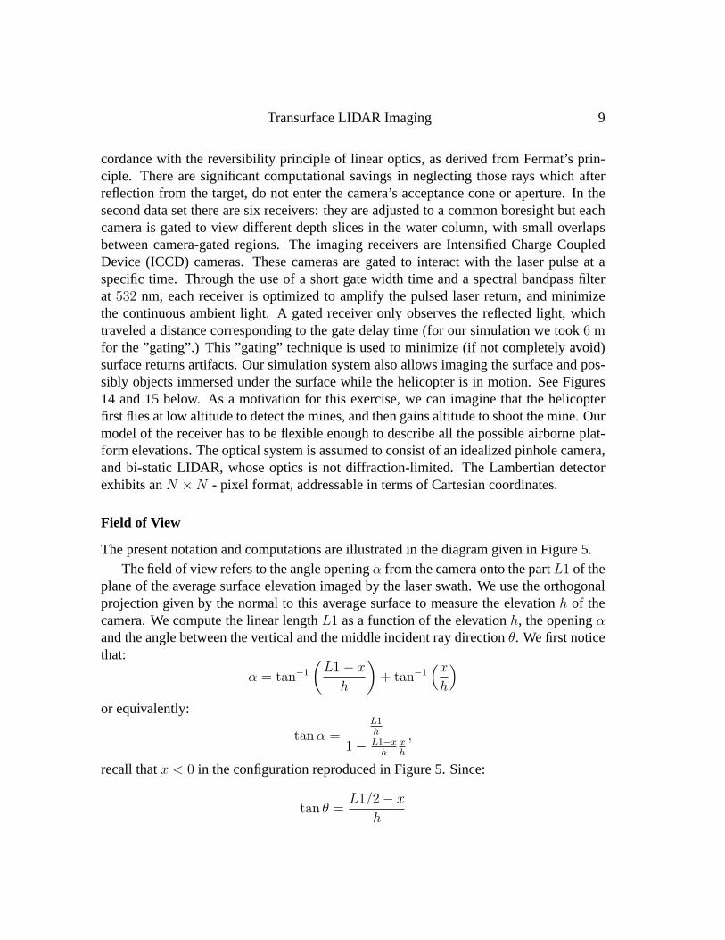
Field of View

The present notation and computations are illustrated in the diagram given in Figure 5.The field of view refers to the angle openingα from the camera onto the partL1 of the

plane of the average surface elevation imaged by the laser swath. We use the orthogonalprojection given by the normal to this average surface to measure the elevationh of thecamera. We compute the linear lengthL1 as a function of the elevationh, the openingαand the angle between the vertical and the middle incident ray directionθ. We first noticethat:

α = tan−1

(L1− x

h

)+ tan−1

(xh

)or equivalently:

tanα =L1h

1− L1−xh

xh

,

recall thatx < 0 in the configuration reproduced in Figure 5. Since:

tan θ =L1/2− x

h


Figure 5: Schematic diagram to illustrate the notation of the field of view discussion.


we can solve forL1 and get:

L1 = 2

(− h

tan(α)+ h

√1 +

1

tan2 α+ tan2 θ

).

We perform the same computation in they-axis direction, using the same openingα, andwe compute the corresponding lengthL2, and we keep only the greatest of the two. Ourcomputation has to be refined if the receiver’s field of viewα is not the same as the laserfield of view. In our simulation, we use the same valueα = 8 deg for both angles. Thisvalue should not be too far from the value used in experiments. Next we need to choosethe rendering of the surface of the water. We choose a fixed set of grid points at thesurface and we only consider the rays (downwelling and upwelling), which go throughthese points. In fact we assign each cell of the camera to a single point of the water surfacegrid. In this way, we do not need to project the image at the water level on the plane ofthe camera sensors.

The camera model

We now review the form of the projection technique from a pinhole camera. This isneeded when we consider that the laser is a source of parallel rays. See [10]. A perspectivetransformation projects3-d points onto a2-d plane. It provides an approximation ofthe way in which a plane image represents a3-d world. Let us assume that the cameracoordinate system(x, y, z) has the image plane as its(x, y) plane, and let the optical axis(established by the center of the lens) be along thez-axis. To be specific we assume thatthe center of the image plane is at the origin, and that the center of the lens is at thepoint with coordinates(0, 0, λ). If the camera is focused on the far field,λ is the focallength of the lens. Next we assume that the camera coordinate system is aligned with theworld coordinate system(X, Y, Z). The coordinates(x, y) of the projection of the point(X,Y, Z) onto the image plane are given by the formulae:

x = λX

λ− Z, y = λ

Y

λ− Z.

Remark 4.1 The homogenous coordinates in the projective space of a point with Carte-sian coordinates(X, Y, Z) are defined as(kX, kY, kZ, k), where k is an arbitrary, nonzeroconstant. Clearly, conversion of homogenous coordinates back to Cartesian coordinatesis accomplished by dividing the first three homogenous coordinates by the fourth.

We define the perspective transformation matrixP as:

P =

1 0 0 00 1 0 00 0 1 00 0 −1/λ 1

.


The corresponding basic mathematical model is based on the assumption that the cameraand the world coordinate systems coincide. We want to consider the more general sit-uation of a world coordinate system(X, Y, Z) used to identify both the camera and3-dpoints in a camera coordinate system(x, y, z). The new assumption is that the camera ismounted on gimbals, allowing pan of an angleθ, and tilt of an angleα. Here, pan is theangle between thex andX axes, and tilt is the angle between thez andZ axes.

Pan angle: < Ox,OX >= θ, Tilt angle: < Oz,OZ >= α.

The goal is to bring the camera and the world coordinate systems into alignment by ap-plying a set of linear transformations. After doing so, we simply apply the perspectivetransformation to obtain the image-plane coordinates for any world point. Translationof the origin of the world coordinate system to the location of the image plane center isaccomplished by using the transformation matrix:

G =

1 0 0 −X0

0 1 0 −Y0

0 0 1 −Z0

0 0 0 1

.In order to pan thex-axis to the desired direction, we rotate it byθ. We proceed similarlyfor the tilt angleα, except for the change in the axis of rotation. The composition of thetwo rotation is given by the single matrix:

R =

cos θ sin θ 0 0

− sin θ cosα cos θ cosα sinα 0sin θ sinα − cos θ sinα cosα 0

0 0 0 1

.So if C denotes the Cartesian coordinates andW the world coordinates, we have:

C = PRGW .

We obtain the Cartesian coordinates (x, y) of the imaged point by dividing the first andsecond components ofC by its fourth. We obtain:

x = λ(X −X0) cos θ + (Y − Y0) sin θ

−(X −X0) sin θ sinα+ (Y − Y0) cos θ sinα− (Z − Z0) cosα+ λ

y = λ−(X −X0) sin θ cosα+ (Y − Y0) cos θ cosα+ (Z − Z0) sinα

−(X −X0) sin θ sinα+ (Y − Y0) cos θ sinα− (Z − Z0) cosα+ λ.

This camera model is very flexible: we just need to know the coordinates of the heli-copter/camera, and the incident ray direction to have all the information we need.


4.3 Light Propagation through the Air/Water Interface

Refraction at the air-sea interface results in focusing and defocusing of both downwellingand upwelling radiations. This effect is commonly observed in every day life, a typicalinstance being the spatial patterns formed at the bottom of a swimming pool on a sunnyday. For upwelling radiation, the image of a submerged object is strongly distorted by therefractive artifacts produced by of the waves.

In this work, we do not consider scattering in the air: we assume that the rays arrivingat, or leaving the air/water interface, travel along straight lines. Also, for this part of theresearch, we assume that each timet, we have a way to compute the surface elevation andthe normal to this surface at each point of the surface above a given grid. We assume thatthe illumination of the surface is such that one ray arrives at each point of the surface grid.Reflection and refraction at a surface can be specular or diffuse. In our case, the process isspecular: the energy of the incident ray is divided solely between reflected and refracteddaughter rays.

Snell’s Law

As explained in [15], the properties of reflected and refracted rays from a level surface aresummarized in Figure 6.

Following Mobley’s book’s convention,ξ′ represents the unit vector along the direc-tion of the incident ray, whileξr andξt denote unit vectors in the directions of the reflectedand transmitted (refracted) rays respectively. The unit normal vector to the interface is de-noted byn. These notation are illustrated in Figure 6.The relevant formulae are reported in Table 2 below. The first row of equations fol-lows from Snell’s Law, wherenw ≈ 1.34 is the refractive index of water. Subsequentrows present equations governing properties of the reflected and refracted daughter rays,specifying the directional vector as well as the incident angles. These equations can beeasily derived using Snell’s law.

AIR-INCIDENT RAYS WATER-INCIDENT RAYS

sin θ′ = nw sin θ nw sin θ′ = sin θξr = ξ′ − 2(ξ′ · n)n ξr = ξ′ − 2(ξ′ · n)n

ξt = (ξ′ − cn)/nw wherec = ξ′ · n−

√(ξ′ · n)2 + n2

w − 1

ξt = nwξ′ − cn where

c = nw(ξ′ · n)−√nw(ξ′ · n)2 − n2

w + 1θr = θ′ = cos−1(ξ′ · n) θr = θ′ = cos−1(ξ′ · n)θt = sin−1(sin θ′/nw) θt = sin−1(sin θ′/nw)

Table 2: Snell’s law formulae


Figure 6: Schematic diagram to illustrate the discussion of Snell’s law.

Fresnel’s Reflectance

Assuming perfect specular returns, the Fresnel’s reflectancer is the fraction of the inci-dent ray’s energy retained by the reflected daughter ray. If we letΦ denote the radiantenergy carried by a single ray, the following equations hold for the radiant energiesΦr

andΦt of the reflected and transmitted rays:

Φr = rΦ and Φt = tΦ

if t = 1− r denotes the transmittance, i.e. the fraction of energy passed to the transmitteddaughter ray (recall that the Fresnel’s reflectancer is a number between0 and1.) Thereflectancer is a function of the incident angleθ′. This function is given, for both theair-incident and the water-incident cases, by Fresnel’s formula:

r(θ′) =1

2

(sin2(θ′ − θt)

sin2(θ′ + θt)+

tan2(θ′ − θt)

tan2(θ′ + θt)

)r(0) =

(nw − 1

nw + 1

)2

As the incident angleθ′ increases from0 deg to 90 deg, Fresnel’s reflectance becomesmore significant until it eventually reaches the maximum value of1. The difference in


refractive indices leads to a higher reflectance for water-incident rays as compared toair- incident rays. In other words, it is much easier for light to enter than to leave theocean. Fresnel’s reflectance equals to1 for a water-incident ray at or beyond the criticalincident angle of48 deg. This phenomenon of total internal reflection greatly influencesthe passage of radiant energy across an air-water. When this critical point is reached, noenergy from the ray can be transmitted from water to air.

4.4 Small Angle Diffusion Approximation in the Water

Like many authors, see for example [13] or [14], we use the small angle diffusion approx-imation introduced by Wells in [22].

4.4.1 The scattering Explanation

Not only is scattering a complex phenomenon, but its effect on imaging also dependsgreatly on the biological and chemical conditions of the ocean. While scattering andabsorption due to natural water are by and large well understood, distortions due to un-derwater organisms and other particles are extremely hard to quantify. Refractive effectsoften appear as spatial feature dissociations (breakup), while multiple scattering tends toproduce resolution degradations and contrast reduction in the received image. Analysisof the propagation of light through water is complicated by multiple scattering and by thestrong forward directivity of each scattering. Only relatively simple imaging systems op-erating over short water paths have been analyzed successfully using the conventional op-tical oceanographic parameters (the attenuation coefficient, the absorption coefficient andthe volume scattering function). This is an active research topic in the field of oceanog-raphy, and has led to the development of various forms of scattering theories. The smallangle scattering approximation is one of them. It is of great importance in many imagingapplications. In this approximation, one circumvents these practical and theoretical dif-ficulties in obtaining analytic solutions to imaging problems, by using a technique wellknown in the analysis of linear electrical and optical systems. It involves the characteriza-tion of the system (optics and water paths) in terms of its response to an impulse of scenereflectance. The output can be expressed as a convolution of the input reflectance distri-bution with the system impulse response function. Alternatively, these operations may beperformed in the Fourier domain. The system spread function is computed as the productof the transmitter spread function and the receiver spread function. Each of these spreadfunctions describes the spreading produced by the optics on a one-way water path. Suchspread functions have been used to predict successfully the performance of several typesof imaging systems over long water paths. We define the two essential water scatteringfunctions: the point spread function PSF and the beam-spread function.

The Beam Spread Function (BSF for short)BSF (θ,Φ, R) is used for the normalizedirradiance distribution on a spherical surface of radiusR centered on the transmitter. The


beamB travels from a sourceS at the origin to its focal point at the rangeR. Irradianceis measured on a small area of the spherical surface at rangeR. See Figure 7 for details.

Figure 7: Beam Spread Function Diagram.

The Point Spread Function (PSF for short)PSF (θ,Φ, R) is used for the apparentnormalized radiance of an unresolved Lambertian source at the position(0, 0, R). Thereceiver is located at the origin and it points to a small areaa of the spherical surface atrangeR. In other words,PSF (θ,Φ, R) is the apparent radiance in the direction(θ,Φ) re-sulting from scattering in the medium of radiance from an unresolved Lambertian sourceat (0, 0, R).In the practical applications we are interested in, the angleΦ is very small, and itwill be convenient to redefineBSF (θ, R) andPSF (θ, R) as the irradiance and radiancevalues present in planes tangent to the spheres at(0, 0, R) for smallθ’s.

Scattering Computations

Because of the symmetric roles played by the PSF and the BSF, we shall only need tocompute the PSF (see Wells’ fundamental paper [22] for a discussion of the reciprocitybetween the PSF and the BSF.) Wells also suggested a simple algebraic form for the scat-tering phase functions(θ), expression which can be analytically integrated, thus allowingfor a straightforward computation of the PSF. The system can also be described in termsof the Mean Transfer Function (MTF for sort) which is obtained from the PSF by Fouriertransform, the latter being implemented with the Fast Fourier Transform since we are


Figure 8: Point Spread Function Diagram.

working on a finite grid. Accordingly:

MTF (ψ) = e−ctebf zD(ψ),

where we follow Wells’ notation with the exception that the range dependencez is fac-tored out of the MTF exponentD(ψ), so thatD depends only on the scattering phaseψ.This exponent is given by the formula:

D(ψ) =1

ψ

∫ ψ

0

Σ(ψ′) dψ′

where:

Σ(ψ) = 2π

∫ 2π

0

s(θ)J0(2πθψ)θ dθ.

In our simulation system, we use the following alternative algebraic form of the scatteringfunction:

s(θ) =s0

θ3/2√θ20 + θ2

for 0 ≤ θ ≤ π, the constants0 being chosen so thatD(0) = Σ(0) = 1, yielding:

MTF (0) = e−(c−bf )z = e−Kdz


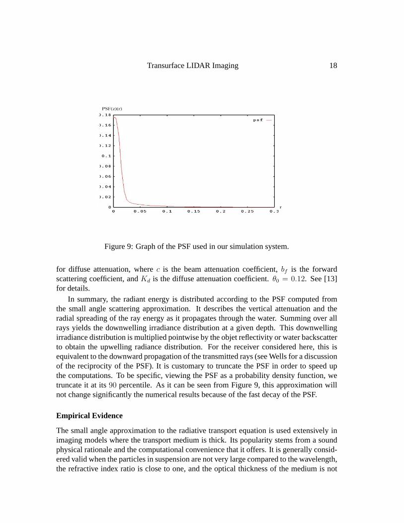
Figure 9: Graph of the PSF used in our simulation system.

for diffuse attenuation, wherec is the beam attenuation coefficient,bf is the forwardscattering coefficient, andKd is the diffuse attenuation coefficient.θ0 = 0.12. See [13]for details.

In summary, the radiant energy is distributed according to the PSF computed fromthe small angle scattering approximation. It describes the vertical attenuation and theradial spreading of the ray energy as it propagates through the water. Summing over allrays yields the downwelling irradiance distribution at a given depth. This downwellingirradiance distribution is multiplied pointwise by the objet reflectivity or water backscatterto obtain the upwelling radiance distribution. For the receiver considered here, this isequivalent to the downward propagation of the transmitted rays (see Wells for a discussionof the reciprocity of the PSF). It is customary to truncate the PSF in order to speed upthe computations. To be specific, viewing the PSF as a probability density function, wetruncate it at its90 percentile. As it can be seen from Figure 9, this approximation willnot change significantly the numerical results because of the fast decay of the PSF.

Empirical Evidence

The small angle approximation to the radiative transport equation is used extensively inimaging models where the transport medium is thick. Its popularity stems from a soundphysical rationale and the computational convenience that it offers. It is generally consid-ered valid when the particles in suspension are not very large compared to the wavelength,the refractive index ratio is close to one, and the optical thickness of the medium is not


too large. But the limits beyond which this approximation becomes unreasonable are notwell understood. We use as a guideline the recent empirical study [20] which is devotedto the quantification of the limits of this approximation validity.

4.5 Target Shape/Reflectivity Adjustment

Our basic assumption is that mines are spheres whose reflectance are diffuse: this meansthat all the incident energy coming into a small area of the surface of a mine, multiplied bythe mine reflectance is equal to the overall reflected energy leaving this area. Moreover,we assume that the reflected energy is the same in all the directions. We shall come backlater to the discussion of the target reflectance.

Figure 10: Projection of the spherical target on a rectangular grid.

In order to make the computation easier, we project the sphere on a rectangular grid(see Figure 10.) We call this grid the target plane. The matrix of the grid points coor-dinates is necessary huge. This is unfortunate because it will be needed later when weinclude the backscattering effects in our simulation. The sharpness of the definition isfree: this is a common technique in computer vision. On the other hand, the discretiza-tion is regular. We will study the incoming light on each square plaquette of the grid.But in order to give to this plane the appearance of a sphere, we need to give to eachsquare element of the plane grid a weight, which is function of the part of the surface of


the sphere, which corresponds to this square plaquette. In order to do so, we perform theprojection as indicated in Figure 11:

Figure 11:2-d details of the projection procedure.

As before we work with an orthogonal set of axes. Working first in thex-direction weget the angleθ and the lengthR′. Doing the same with the other axis, we getR′′ and theangleψ. Then we are able to compute the areaA, which is the projection of the square[i, i+ 1]× [j, j + 1] on the sphere. We will call this area ponder.

The ponder will be multiplied by the target reflectance. Since all the incident energy(coming into a small area on the surface of the3-d target) multiplied by the target re-flectance is equal to all the reflected energy leaving this area, which is the same in all thedirections, our plane representation takes into account the real area of each element of ourmatrix.

A = ponder(i, j) ≈ (θR′)(ψR′′)

≈ R′R′′∣∣∣∣sin−1 (i+ 1)d

R′′ − sin−1 jd

R′′

∣∣∣∣ ∣∣∣∣sin−1 (j + 1)d

R′ − sin−1 jd

R′

∣∣∣∣Using this weighting technique, our effective target does look like a3-d sphere eventhough it is only a2-d plane disk. To complete the illusion we need to modify the rulesgoverning the reflection of the incident rays. Consequently, if the incident ray direction isnot vertical (vertical rays are the only ones reflected in the same way whether the target is


Figure 12: Ponder function for a quarter of a circular mine.

a sphere or a horizontal plane), we change artificially the target plane to fool the ray intobelieving that it hit a spherical target. A simple3-d-geometric transformation can be usedto do the trick. The illusion is satisfactory and the computations are still much lighter thanthose needed to consider a real3-d spherical model for the target.

Remark 4.2 At this stage it is useful to make sure that there is no ambiguity in the ter-minology used throughout this report. We call incident ray direction the direction of thecentral ray of the laser. When this ray is refracted at the air/water interface, we call itthe refracted incident ray direction. It gives us the average direction of the downwellingrays in the water, and their intersection with the target plane gives us the average positionof the center of the spot of light at this level. The quality of this approximation dependsheavily on the specific realization of the water surface, and unfortunately, it sometimesgives wrong results. Despite these occasional problems, it will be good enough for ourpurposes. The alternative was to consider the incident ray direction after being refractedby a quiet water surface. This alternative was considered inadequate because of the pres-ence of big gravity waves, which shift horizontally the location of the light spot in thetarget plane level.

Our first simulation system was based on the considerations presented so far. It wasquite adequate for the simulation of images and video sequences of the type of the firstdata set. The first two examples presented in the section on experimental results in Sec-tion 5, were generated with this version of our simulator. The last two sections describe


improvements needed to make our system capable of producing realistic simulations ofexperiments such as those leading to the second data set.

4.6 Backscattering in the Gated Region

We now explain how we included backscattering effects in our imaging system. Since wecompute only once the PSF for each image, we cannot use the model of [13] and [14],which would require too much computing time. Instead we choose to use an effectivereflectanceR:

R =sb2K

(1− e−2Kd∆Zg)

on the target plane, wheresb ≈ πs(π) ands is the scattering function defined earlier,Kd

is as before the diffuse attenuation coefficient, and∆Zg is the width of the gate.

Figure 13: Diagram explaining the computation of the effective reflectance.

In this way, the reflectance coefficientR depends only upon the gating (i.e. the permis-sible travel time of the rays from the source and to the sensor) and on the characteristicsof the water turbidity. In words, we combine all the backscattering in the gated regioninto a cumulative effect, which is incorporated in the model as the effective reflectanceof the plane at the bottom of the gate. We add this reflectance to the reflectance of the


target, and we apply the same tools as earlier: we use the PSF to describe the scatteringand the diffusion for each ray, even those that are far from the target: backscattering iseverywhere. We compute first the incoming light on the target plane (i.e. the plane at thebottom of the gate), and then we multiply the incoming luminance of each element of ourdiscretization of the target plane by the reflectance distribution we just computed. We canthen produce an image of the target plane and the target itself seen from the water justabove this plane. We use again the PSF to compute the upwelling rays, and we take intoaccount the refraction at the water-air interface as before. Finally we obtained the desired(distorted) image.

Notice that the equation giving the effective reflectance due to backscattering does notdepend upon the actual travel time of each ray but that it only depends upon the thicknessof the gate. It does not enter into the computation of the PSF.

4.7 The Sensor Poisson Shot Noise

The receiver comprises CCD sensors. The emission of photons from any source is arandom process and the number of photogenerated carriers collected in a potential wellin a given time interval of lengthT , is a random variable. The standard deviation of thisrandom variable characterizes the (quantum) photon noise. Since the number of photonsemitted follows a Poisson distribution, the standard deviation of the number of chargescollected equals the square root of the mean and thusNnoise=

√Ns. This noise source

is of course a fundamental limitation in most applications since it is a property of lightitself, not the image sensor. This limitation tends to become serious only under conditionsof low scene contrast, as it is often the case in imaging at low light levels and like in ourcase. We have:

Ns =HSAT

q

whereH is the image irradiance inW/m2, S is the effective responsivity inA/W (thetypical for an ideal receiver being238 mA/W ), A is the geometric area of each cell, andq the charge of the electron. In order to get a feel for this irradiance, we reproduce inTable 3 the figures computed for some astronomical objects:

Irradiance (inW/m2)

Starlight 5.10−5

Full moon 5.10−3

Twilight 5.10−3

Table 3: Examples of Physical Irradiances

Since we do not have enough information on the physical characteristics of the laser


and the receiver used in the experiments, we do not have exact values for image irradiance.For the numerical experiments we performed withNs, we choseNs from 0 to 13. Thecovariance and the mean of the random variable are the numberNs of charges collectedin this pixel. The new pixel value isn, whose probability is:

p(n) =Nns

n!e−Ns .

We will apply this noise to the final images. For the computation, we just need a randomnumber generator.

5 Simulation Results

We present some of the results obtained with the simulation system described in the pre-vious section, our main goal being the comparison with the experimental data introducedin the first section. Recall that the fixed images shown below are in fact frames fromanimations (animated GIF files) which can be viewed at the URL:

http://www.princeton.edu/ rcarmona .

Example 1

For this first example, the ocean surface was generated with a Phillips spectrum and thefollowing parameters:

� The wind speed was set to5.0 m/s� The maximum wave elevation was setto0.1 m� The helicopter flies up from16 m to66 m� A spherical mine of radius0.3 m was present5 m below the surface� The incident rays were vertical� The truncation of the PSF was at its95 percentile

The following sequence of images was produced by a simulation of the elevation ofthe helicopter, without any backscattering or shot noise. We also consider the laser asa group of parallel incident rays. This result shows that our simulation system (evenwithout the backscattering and shot noise effects) is adequate to produce images similarto the images of the first data set. Moreover, it also shows that it can handle motion of theimaging platform.

Example 2

The parameters used to produce the next example are very similar, except for the fact thatthe helicopter motion is not necessarily vertical. The output includes the surface of the sea


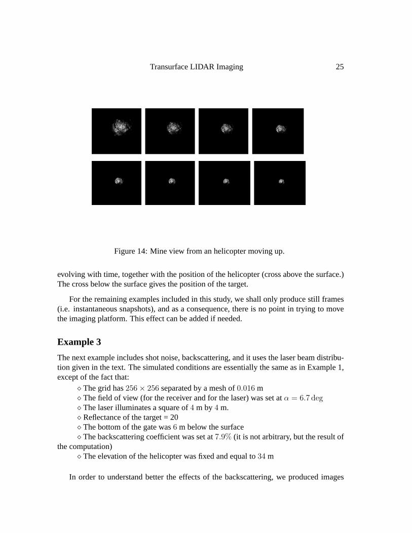
Figure 14: Mine view from an helicopter moving up.

evolving with time, together with the position of the helicopter (cross above the surface.)The cross below the surface gives the position of the target.

For the remaining examples included in this study, we shall only produce still frames(i.e. instantaneous snapshots), and as a consequence, there is no point in trying to movethe imaging platform. This effect can be added if needed.

Example 3

The next example includes shot noise, backscattering, and it uses the laser beam distribu-tion given in the text. The simulated conditions are essentially the same as in Example 1,except of the fact that:

� The grid has256× 256 separated by a mesh of0.016 m� The field of view (for the receiver and for the laser) was set atα = 6.7 deg� The laser illuminates a square of4 m by4 m.� Reflectance of the target = 20� The bottom of the gate was6 m below the surface� The backscattering coefficient was set at7.9% (it is not arbitrary, but the result of

the computation)� The elevation of the helicopter was fixed and equal to34 m

In order to understand better the effects of the backscattering, we produced images


Figure 15: The bottom images show the ocean surface together position of the helicopter,and the top panes show the image of the mine as viewed from the helicopter moving up.


with a mine (left column of Figure 16), and without a mine (right column of Figure 16).One can clearly see the differences due to the presence of a mine.

Figure 16: The images on the left contain a mine while the images on the right don’t.

More images generated in this way shows that how apparent the mine is in the imagedepends strongly on the relative values of the target reflectance and the water turbidity asencapsulated by the backscattering coefficient. The mines can easily be seen in Figure16 because the target reflectance is20% and the backscattering coefficient is7.9%. Realexperimental data suffer from the same problems: the backscattering affects significantlythe detection.

Example 4

Finally for this last example, we choose to illustrate the effects of the ”gating” just belowthe target. The goal of this experiment is to see the shadow of the target. We take the sameocean surface, and the same target properties as above. The depth of the target plane is3 m and the gating depth9 m and we produce images as seen from the helicopter. The


image on the left of Figure 17 was produced with a target while the image on the rightwas produced without a target.

Figure 17: Simulation of the gating effect.

We can see the shadow and the influence of the target for the upwelling rays anddownwelling rays in the left image. The right image is a reference of the same gatingimage (with backscattering....) but without the target above. This example shows thelimits of our methodology and presumably of the computation of the PSF and the effectivebackscattering. Indeed, these images are not very realistic. The shadow is too big, with toomuch contrast: the multiple backscattering must have an influence despite the presence ofthe target.

6 Conclusion

This report records our first attempt at deriving a real-time imaging system for the de-tection and identification of underwater objects with an airborne LIDAR system. Imple-mentations of a wave simulation model together with an imaging algorithm have beencompleted and experimental results have been presented and analyzed. The lack of ob-jective metrics to quantify the quality of the results is the Achilles heel of simulation.


Nevertheless, the images produced by our system are very satisfactory. Moreover, thedetection results obtained in [4] confirm its usefulness. In fact, because of its modularity,its usefulness should not be limited to the detection of moored mines. Many other appli-cations in search and rescue, whether they take place in the ocean, in a lake, a pond or apool, should benefit from the tools developed in this study.

Future research should aim at further developing this imaging tool in several direc-tions, robustness being an obvious one.

But the ultimate challenge remains the derivation of a stable inversion algorithm,which will lead to a reliable underwater object detection and identification device.

Acknowledgments:This work would not have been possible without the contributions of several individ-

uals who have been instrumental in speeding up our learning curve. They include DickLau and Nancy Swanson for providing access to the data and to funding sources, and formany enlightening conversations on the real life experimental conditions. We are alsograteful to Steve Moran from Kaman Aerospace for several discussions of the same vein.Finally, we would like to thank Annette Fung for her contribution at a very early stage ofthe project.

References

[1] R. J. Adler (1981): The Geometry of Random Fields. John Wiley & Sons. NewYork, NY

[2] J.D.E.Beynon and D.R.Lamb: Charge-Coupled devices and their applications, McGraw Hill

[3] R. Carmona and Y. Picard (1999): Gibbs Fields for Conditional Simulation of Ran-dom Fields. Tech.Rep. ORFE Dept. Princeton University.

[4] R. Carmona and L.Wang (2000): Lidar Detection of Moored Mines. Tech. Rep.ORFE Dept, Princeton University.

[5] R. Cipolla and P. Giblin (2000): Visual Motion of Curves and Surfaces. CambridgeUniv. Press. Cambridge UK

[6] Costal Systems Station:Magic Lantern (ML) Automatic Recognition (ATR)Database Report, Jan. 1996.

[7] N.A. Cressie (1993): Statistics for Spatial Data. John Wiley & Sons, New York, NY

[8] S. Frimpong and P.K Achireko (1998): Conditional LAS stochastic simulation ofregionalized variables in random fields.Computational Geosciences2, 37-45.


[9] A.N.Fung (1998): Imaging through an ocean surface: a simulation approach. SeniorThesis, ORFE Dept, Princeton University

[10] R.C. Gonzales and R.E. Woods (1992): Digital Image Processing, Addison WesleyPub. Cpy

[11] A.G. Journel and C.G. Huijbregts (1978): Mining Geostatistics.Academic PressNew Yourk, NY.

[12] P. Liu and R.A. Kruger (1994): Semianalytical approach to pulsed light propagationin scattering and absorbing media.Optical Engineering,33

[13] J.W. McLean and J.D.Freeman (1996): Effects of ocean waves on airborn lidarimaging.Applied Optics35#118 pp. 3261-3269.

[14] L.E. Mertens and F.S. Replogle, Jr (1977): Use of point spread and beam spreadfunctions for analysis of imaging systems in water

[15] C.D. Mobley (1994): Light and Water. Academic Press, New York, NY

[16] M.S. Schmalz (1990): Rectification of refractively-distorted imagery acquiredthrough the sea surface: an Image Algebra formulation,SPIE Image Algebra andMorphological image Processing

[17] M. Shinozuka and R. Zhang (1996): Equivalence between kriging and CPDF meth-ods for conditional simulation.J. of Eng. Mechanics122(6), 530-538.

[18] M. Shinozuka, R. Zhang and M. Oshiya (1996): Conditional Simulation Tech-niques: Recent Developments and Applications.in IASSAR report on Computa-tional Stochastic MechanicsSect. 1.6 pp. 224-226.

[19] P-T. D. Spanos (1983): ARMA Algorithms for Ocean Wave Modeling.J. EnergyResources Technology105,300-309.

[20] N.L. Swanson, V.M. Gehman, B.D. Billard and T.L. Gennaro (2000): Limits of theSmall Angle Approximation to the Radiative Transport Equation.NSWC preprintDahlgren VA.

[21] R.E. Walker (1994): Marine Light field Statistics. Jon Wiley & Sons, New York,NY.

[22] H.G. Wells (1973): theory of small angle scattering,AGRAD Lect. Ser.61

lidar imaging through the ocean surface - princeton universityrcarmona/download/image/mine1.pdf ·...

Documents