LiDAR IMAGERY EMPLOYED IN CAROLINA BAYS RESEARCH

Demonstrating Integration withGoogle Earth Virtual Globe

Abstract No: 1767382010 GSA Annual Meeting31 October – 3 November Denver, Colorado USA

Michael E. DaviasJeanette L. Gilbride

?

Photo Courtesy of George Howard

Myrtle Beach, SC

©Fairchild Aerial Surveys for the Ocean Forest Company: Aerial view taken in 1930 (12x8 km)

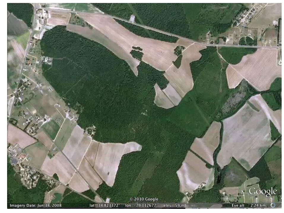
GE Imagery (1999), St. Pauls, NC

GE Imagery Wilmington, NC

Rationale

“No one has yet invented an explanation which will fully account for all the facts observed”

Douglas Johnson, 1942The Origin of the Carolina Bays

Bubble Foam

Research Requirements

• Create Comprehensive Catalogue of Carolina bay landforms• Triangulation Network requires broad spatial distribution of bays & alignments• Integrate with Google Earth Virtual Globe

Carolina bay Orientation – Johnson (1942)Carolina bay Orientation - Eyton & Parkhurst (1975) Carolina bay Orientation – Johnson (1942)

Tools & Resources

• USGS 1/9 Arc-second National Elevation Data• Nebraska Department of Natural Resources

LiDAR data• Global Mapper commercial GIS program

– Loads many type of data, we use Arc-Grid here– Save as JPG or TIFF– Save as Keyhole Markup language (KML) data file

• Google Earth loads Global Mapper KML– Automatically aligns on virtual globe– Allows for capture of planform geospatial metrics

1/9 arc second LiDAR-derived Data

Nebraska DNR

USGS NED

LiDAR Generation Process

LiDAR Generation Process

LiDAR Generation Process

Elevation Profiles

Nebraska Bays Elevation Profile

515 m 510 m 506 m 505 mAMSL

~ 10 m rim height on 2 km bay

LiDAR Generation Process

LiDAR Integration with Google Earth

Blanket Artifacts – Daughter Bubbles

Antecedent Channels

Double-bay Wall

Lacustrine Bathtub Rings

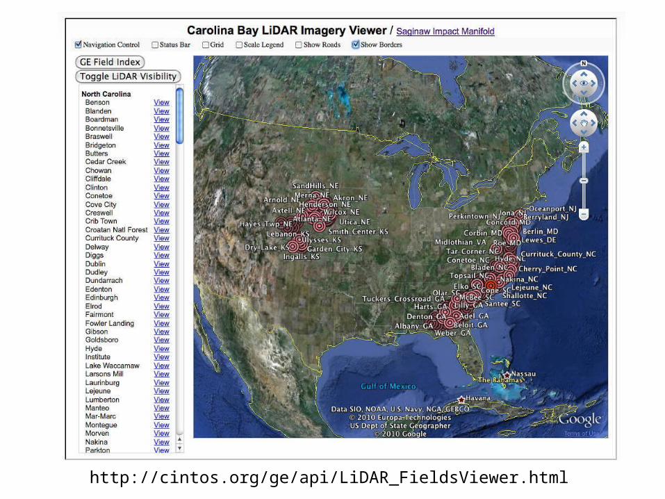
LiDAR Integration with Google Earth

http://cintos.org/ge/api/LiDAR_FieldsViewer.html

LiDAR Integration with Google Earth

http://cintos.org/ge/api/LiDAR_FieldsViewer.html

Capturing Alignment with Overlay

Planform – New Image Overlay

Planform Overlay

Overlay Given a Name

KML Meta Data in Overlay

• <GroundOverlay>• <name>bay_B0355</name>• <Icon>• <href>http://cintos.org/ge/overlays/bay_Prototype.png</href>• <viewBoundScale>0.75</viewBoundScale>• </Icon>• <LatLonBox>• <north>34.63252148936107</north>• <south>34.61506906232364</south>• <east>-79.57293257637467</east>• <west>-79.58581679997867</west>• <rotation>-135.2369396039304</rotation>• </LatLonBox>• </GroundOverlay>

Survey, bay-by-bay

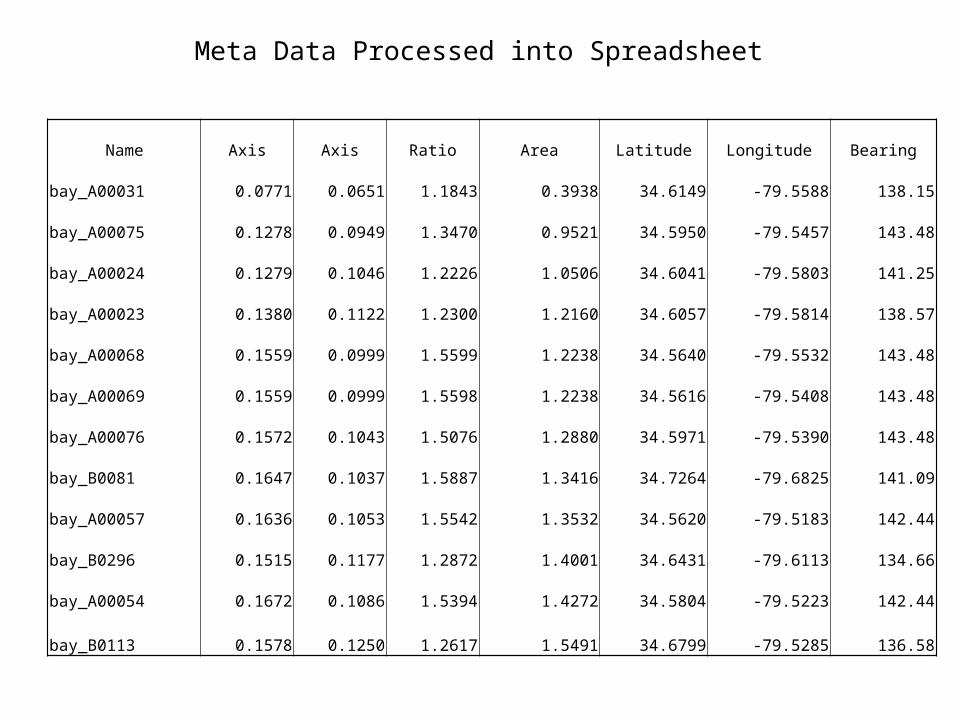
Meta Data Processed into Spreadsheet

Name Axis Axis Ratio Area Latitude Longitude Bearing

bay_A00031 0.0771 0.0651 1.1843 0.3938 34.6149 -79.5588 138.15

bay_A00075 0.1278 0.0949 1.3470 0.9521 34.5950 -79.5457 143.48

bay_A00024 0.1279 0.1046 1.2226 1.0506 34.6041 -79.5803 141.25

bay_A00023 0.1380 0.1122 1.2300 1.2160 34.6057 -79.5814 138.57

bay_A00068 0.1559 0.0999 1.5599 1.2238 34.5640 -79.5532 143.48

bay_A00069 0.1559 0.0999 1.5598 1.2238 34.5616 -79.5408 143.48

bay_A00076 0.1572 0.1043 1.5076 1.2880 34.5971 -79.5390 143.48

bay_B0081 0.1647 0.1037 1.5887 1.3416 34.7264 -79.6825 141.09

bay_A00057 0.1636 0.1053 1.5542 1.3532 34.5620 -79.5183 142.44

bay_B0296 0.1515 0.1177 1.2872 1.4001 34.6431 -79.6113 134.66

bay_A00054 0.1672 0.1086 1.5394 1.4272 34.5804 -79.5223 142.44

bay_B0113 0.1578 0.1250 1.2617 1.5491 34.6799 -79.5285 136.58

Survey Graphs

Triangulation Mash-Up On Virtual Globe

Summary

• Integrated LiDAR DEM images into Google Earth• Identified and Documented ~ 250 Fields of Bays

– Locations– Inferred Arrival Bearings– LiDAR Imagery

• Captured Individual bay Metrics– Location– Major & Minor Axis

• Size• Elongation ratio

– Orientation

• Correlated Alignments using Java Calculator

?

Correlating Bearings

Geospatial Distribution Test

Round & Squashed Bays

Western Bays

Rationale

“No one has yet invented an explanation which will fully account for all the facts observed”

Douglas Johnson, 1942

“…claims of impact origins have been mostly banished from the refereed literature”

Anonymous GRL Reviewer, 2010

LIDAR IMAGERY EMPLOYED IN CAROLINA BAYS RESEARCHAbstract ID#: 176738

Photographs of the Carolina bays have been available from the air since the early 1930’s. Those early images sparked extensive research into their genesis, but they reveal only a small part of their unique planforms. Digital elevation maps (DEM) created with today’s Laser Imaging and Range Detection (LiDAR) systems accentuates their already-stunning visual presentation, allowing for the identification and classification of even greater quantities of these shallow basins across North America.

Our research was enabled to a large part by the facilities and satellite imagery of the Google Earth (GE) Geographic Information System (GIS). The Global Mapper GIS application was used to generate LiDAR image overlays for visualization in Google Earth, using 1/9 arc-second resolution DEM data from the United States Geological Survey (USGS). Using these facilities, a survey was undertaken to catalogue the extent of Carolina bays, indexed as localized “fields”.

Estimations of the bays’ numerical quantity extends into the hundreds of thousands, therefore no attempt was made to identify all such landforms; instead each field was selected to be rigorously representative of the distribution in a given locale. The data is primarily used in a geospatial analysis, attempting to correlate the bays' orientations in a triangulation network. Identifying Carolina bays on the costal plain is straight forward, given their solid identification, however bay planforms tend towards a circular presentation in the northern and southern extremes of their geographic extent, presenting challenges. Also challenging is the rougher terrain seen when moving inland. We suspect that access to high resolution LiDAR DEMs in more regions would aid in expanding the bays’ identified range.

While there is much research discussing Carolina bays in the east, there are significant quantities of aligned, oval basins in the Midwest. These basins are aligned SW NE, and are considered to be vital components of the triangulation ➔network. The survey resulted in a catalogue of ~220 fields of Carolina bays, managed in a Keyhole Markup Language (kml) metadata file. The catalogue of LiDAR images is available for interactive visualization using the GE-GIS using the kml file available at http://cintos.org/ge/SaginawKML/Distal_Ejecta_Fields.kmz.