Journal of Machine Learning Research 9 (2008) 1871-1874 Submitted 5/08; Published 8/08

LIBLINEAR: A Library for Large Linear Classification

Rong-En Fan b90098@csie.ntu.edu.tw

Kai-Wei Chang b92084@csie.ntu.edu.tw

Cho-Jui Hsieh b92085@csie.ntu.edu.tw

Xiang-Rui Wang r95073@csie.ntu.edu.tw

Chih-Jen Lin cjlin@csie.ntu.edu.tw

Department of Computer Science

National Taiwan University

Taipei 106, Taiwan

Last modified: December 8, 2017

Editor: Soeren Sonnenburg

Abstract

LIBLINEAR is an open source library for large-scale linear classification. It supports logisticregression and linear support vector machines. We provide easy-to-use command-line toolsand library calls for users and developers. Comprehensive documents are available for bothbeginners and advanced users. Experiments demonstrate that LIBLINEAR is very efficienton large sparse data sets.

Keywords: large-scale linear classification, logistic regression, support vector machines,open source, machine learning

1. Introduction

Solving large-scale classification problems is crucial in many applications such as text clas-sification. Linear classification has become one of the most promising learning techniquesfor large sparse data with a huge number of instances and features. We develop LIBLINEARas an easy-to-use tool to deal with such data. It supports L2-regularized logistic regression(LR), L2-loss and L1-loss linear support vector machines (SVMs) (Boser et al., 1992). Itinherits many features of the popular SVM library LIBSVM (Chang and Lin, 2011) such assimple usage, rich documentation, and open source license (the BSD license1). LIBLINEARis very efficient for training large-scale problems. For example, it takes only several secondsto train a text classification problem from the Reuters Corpus Volume 1 (rcv1) that has morethan 600,000 examples. For the same task, a general SVM solver such as LIBSVM wouldtake several hours. Moreover, LIBLINEAR is competitive with or even faster than state of theart linear classifiers such as Pegasos (Shalev-Shwartz et al., 2007) and SVMperf (Joachims,2006). The software is available at http://www.csie.ntu.edu.tw/~cjlin/liblinear.

This article is organized as follows. In Sections 2 and 3, we discuss the design andimplementation of LIBLINEAR. We show the performance comparisons in Section 4. Closingremarks are in Section 5.

1. The New BSD license approved by the Open Source Initiative.

c©2008 Rong-En Fan, Kai-Wei Chang, Cho-Jui Hsieh, Xiang-Rui Wang and Chih-Jen Lin.

Fan, Chang, Hsieh, Wang and Lin

2. Large Linear Classification (Binary and Multi-class)

LIBLINEAR supports two popular binary linear classifiers: LR and linear SVM. Given a setof instance-label pairs (xi, yi), i = 1, . . . , l, xi ∈ Rn, yi ∈ {−1,+1}, both methods solve thefollowing unconstrained optimization problem with different loss functions ξ(w;xi, yi):

minw

1

2wTw + C

∑l

i=1ξ(w;xi, yi), (1)

where C > 0 is a penalty parameter. For SVM, the two common loss functions are max(1−yiw

Txi, 0) and max(1−yiwTxi, 0)2. The former is referred to as L1-SVM, while the latter is

L2-SVM. For LR, the loss function is log(1+e−yiwTxi), which is derived from a probabilistic

model. In some cases, the discriminant function of the classifier includes a bias term, b.LIBLINEAR handles this term by augmenting the vector w and each instance xi with anadditional dimension: wT ← [wT , b],xTi ← [xTi , B], where B is a constant specified bythe user. The approach for L1-SVM and L2-SVM is a coordinate descent method (Hsiehet al., 2008). For LR and also L2-SVM, LIBLINEAR implements a trust region Newtonmethod (Lin et al., 2008). The Appendix of our SVM guide2 discusses when to use whichmethod. In the testing phase, we predict a data point x as positive if wTx > 0, andnegative otherwise. For multi-class problems, we implement the one-vs-the-rest strategyand a method by Crammer and Singer. Details are in Keerthi et al. (2008).

3. The Software Package

The LIBLINEAR package includes a library and command-line tools for the learning task.The design is highly inspired by the LIBSVM package. They share similar usage as well asapplication program interfaces (APIs), so users/developers can easily use both packages.However, their models after training are quite different (in particular, LIBLINEAR stores win the model, but LIBSVM does not.). Because of such differences, we decide not to combinethese two packages together. In this section, we show various aspects of LIBLINEAR.

3.1 Practical Usage

To illustrate the training and testing procedure, we take the data set news20,3 which hasmore than one million features. We use the default classifier L2-SVM.

$ train news20.binary.tr

[output skipped]

$ predict news20.binary.t news20.binary.tr.model prediction

Accuracy = 96.575% (3863/4000)

The whole procedure (training and testing) takes less than 15 seconds on a modern com-puter. The training time without including disk I/O is less than one second. Beyond thissimple way of running LIBLINEAR, several parameters are available for advanced use. Forexample, one may specify a parameter to obtain probability outputs for logistic regression.Details can be found in the README file.

2. The guide can be found at http://www.csie.ntu.edu.tw/~cjlin/papers/guide/guide.pdf.3. This is the news20.binary set from http://www.csie.ntu.edu.tw/~cjlin/libsvmtools/datasets. We

use a 80/20 split for training and testing.

1872

LIBLINEAR: A Library for Large Linear Classification

3.2 Documentation

The LIBLINEAR package comes with plenty of documentation. The README file describes theinstallation process, command-line usage, and the library calls. Users can read the “QuickStart” section, and begin within a few minutes. For developers who use LIBLINEAR in theirsoftware, the API document is in the “Library Usage” section. All the interface functionsand related data structures are explained in detail. Programs train.c and predict.c aregood examples of using LIBLINEAR APIs. If the README file does not give the informationusers want, they can check the online FAQ page.4 In addition to software documentation,theoretical properties of the algorithms and comparisons to other methods are in Lin et al.(2008) and Hsieh et al. (2008). The authors are also willing to answer any further questions.

3.3 Design

The main design principle is to keep the whole package as simple as possible while makingthe source codes easy to read and maintain. Files in LIBLINEAR can be separated intosource files, pre-built binaries, documentation, and language bindings. All source codesfollow the C/C++ standard, and there is no dependency on external libraries. Therefore,LIBLINEAR can run on almost every platform. We provide a simple Makefile to compilethe package from source codes. For Windows users, we include pre-built binaries.

Library calls are implemented in the file linear.cpp. The train() function trains aclassifier on the given data and the predict() function predicts a given instance. To handlemulti-class problems via the one-vs-the-rest strategy, train() conducts several binary clas-sifications, each of which is by calling the train one() function. train one() then invokesthe solver of users’ choice. Implementations follow the algorithm descriptions in Lin et al.(2008) and Hsieh et al. (2008). As LIBLINEAR is written in a modular way, a new solvercan be easily plugged in. This makes LIBLINEAR not only a machine learning tool but alsoan experimental platform.

Making extensions of LIBLINEAR to languages other than C/C++ is easy. Followingthe same setting of the LIBSVM MATLAB/Octave interface, we have a MATLAB/Octaveextension available within the package. Many tools designed for LIBSVM can be reused withsmall modifications. Some examples are the parameter selection tool and the data formatchecking tool.

4. Comparison

Due to space limitation, we skip here the full details, which are in Lin et al. (2008) and Hsiehet al. (2008). We only demonstrate that LIBLINEAR quickly reaches the testing accuracycorresponding to the optimal solution of (1). We conduct five-fold cross validation to selectthe best parameter C for each learning method (L1-SVM, L2-SVM, LR); then we train onthe whole training set and predict the testing set. Figure 1 shows the comparison betweenLIBLINEAR and two state of the art L1-SVM solvers: Pegasos (Shalev-Shwartz et al., 2007)and SVMperf (Joachims, 2006). Clearly, LIBLINEAR is efficient.

To make the comparison reproducible, codes used for experiments in Lin et al. (2008)and Hsieh et al. (2008) are available at the LIBLINEAR web page.

4. FAQ can be found at http://www.csie.ntu.edu.tw/~cjlin/liblinear/FAQ.html.

1873

Fan, Chang, Hsieh, Wang and Lin

(a) news20, l: 19,996, n: 1,355,191, #nz: 9,097,916 (b) rcv1, l: 677,399, n: 47,236, #nz: 156,436,656

Figure 1: Testing accuracy versus training time (in seconds). Data statistics are listed afterthe data set name. l: number of instances, n: number of features, #nz: numberof nonzero feature values. We split each set to 4/5 training and 1/5 testing.

5. Conclusions

LIBLINEAR is a simple and easy-to-use open source package for large linear classification.Experiments and analysis in Lin et al. (2008), Hsieh et al. (2008) and Keerthi et al. (2008)conclude that solvers in LIBLINEAR perform well in practice and have good theoreticalproperties. LIBLINEAR is still being improved by new research results and suggestions fromusers. The ultimate goal is to make easy learning with huge data possible.

References

B. E. Boser, I. Guyon, and V. Vapnik. A training algorithm for optimal margin classifiers.In COLT, 1992.

C.-C. Chang and C.-J. Lin. LIBSVM: A library for support vector machines. ACM TIST,2(3):27:1–27:27, 2011.

C.-J. Hsieh, K.-W. Chang, C.-J. Lin, S. S. Keerthi, and S. Sundararajan. A dual coordinatedescent method for large-scale linear SVM. In ICML, 2008.

T. Joachims. Training linear SVMs in linear time. In ACM KDD, 2006.

S. S. Keerthi, S. Sundararajan, K.-W. Chang, C.-J. Hsieh, and C.-J. Lin. A sequential dualmethod for large scale multi-class linear SVMs. In KDD, 2008.

C.-J. Lin, R. C. Weng, and S. S. Keerthi. Trust region Newton method for large-scalelogistic regression. JMLR, 9:627–650, 2008.

S. Shalev-Shwartz, Y. Singer, and N. Srebro. Pegasos: primal estimated sub-gradient solverfor SVM. In ICML, 2007.

1874

LIBLINEAR: A Library for Large Linear Classification

Acknowledgments

This work was supported in part by the National Science Council of Taiwan via the grantNSC 95-2221-E-002-205-MY3.

Appendix: Implementation Details and Practical Guide

Appendix A. Formulations

This section briefly describes classifiers supported in LIBLINEAR. Given training vectorsxi ∈ Rn, i = 1, . . . , l in two class, and a vector y ∈ Rl such that yi = {1,−1}, a linearclassifier generates a weight vector w as the model. The decision function is

sgn(wTx

).

LIBLINEAR allows the classifier to include a bias term b. See Section 2 for details.

A.1 L2-regularized L1- and L2-loss Support Vector Classification

L2-regularized L1-loss SVC solves the following primal problem:

minw

1

2wTw + C

l∑i=1

(max(0, 1− yiwTxi)),

whereas L2-regularized L2-loss SVC solves the following primal problem:

minw

1

2wTw + C

l∑i=1

(max(0, 1− yiwTxi))2. (2)

Their dual forms are:

minα

1

2αT Qα− eTα

subject to 0 ≤ αi ≤ U, i = 1, . . . , l.

where e is the vector of all ones, Q = Q+D, D is a diagonal matrix, and Qij = yiyjxTi xj .

For L1-loss SVC, U = C and Dii = 0, ∀i. For L2-loss SVC, U =∞ and Dii = 1/(2C), ∀i.

A.2 L2-regularized Logistic Regression

L2-regularized LR solves the following unconstrained optimization problem:

minw

1

2wTw + C

l∑i=1

log(1 + e−yiwTxi). (3)

Its dual form is:

minα

1

2αTQα+

∑i:αi>0

αi logαi +∑

i:αi<C

(C − αi) log(C − αi)−l∑

i=1

C logC

subject to 0 ≤ αi ≤ C, i = 1, . . . , l.

(4)

A.1

Fan, Chang, Hsieh, Wang and Lin

A.3 L1-regularized L2-loss Support Vector Classification

L1 regularization generates a sparse solution w. L1-regularized L2-loss SVC solves thefollowing primal problem:

minw

‖w‖1 + Cl∑

i=1

(max(0, 1− yiwTxi))2. (5)

where ‖ · ‖1 denotes the 1-norm.

A.4 L1-regularized Logistic Regression

L1-regularized LR solves the following unconstrained optimization problem:

minw

‖w‖1 + C

l∑i=1

log(1 + e−yiwTxi). (6)

where ‖ · ‖1 denotes the 1-norm.

A.5 L2-regularized L1- and L2-loss Support Vector Regression

Support vector regression (SVR) considers a problem similar to (1), but yi is a real valueinstead of +1 or −1. L2-regularized SVR solves the following primal problems:

minw

1

2wTw +

{C∑l

i=1(max(0, |yi −wTxi| − ε)) if using L1 loss,

C∑l

i=1(max(0, |yi −wTxi| − ε))2 if using L2 loss,

where ε ≥ 0 is a parameter to specify the sensitiveness of the loss.Their dual forms are:

minα+,α−

1

2

[α+ α−

] [ Q −Q−Q Q

] [α+

α−

]− yT (α+ −α−) + εeT (α+ +α−)

subject to 0 ≤ α+i , α

−i ≤ U, i = 1, . . . , l,

(7)

where e is the vector of all ones, Q = Q+D, Q ∈ Rl×l is a matrix with Qij ≡ xTi xj , D isa diagonal matrix,

Dii =

{01

2C

, and U =

{C if using L1-loss SVR,

∞ if using L2-loss SVR.

Rather than (7), in LIBLINEAR, we consider the following problem.

minβ

1

2βT Qβ − yTβ + ε‖β‖1

subject to − U ≤ βi ≤ U, i = 1, . . . , l,

(8)

where β ∈ Rl and ‖ · ‖1 denotes the 1-norm. It can be shown that an optimal solution of(8) leads to the following optimal solution of (7).

α+i ≡ max(βi, 0) and α−i ≡ max(−βi, 0).

A.2

LIBLINEAR: A Library for Large Linear Classification

Appendix B. L2-regularized L1- and L2-loss SVM (Solving Dual)

See Hsieh et al. (2008) for details of a dual coordinate descent method.

Appendix C. L2-regularized Logistic Regression (Solving Primal)

See Lin et al. (2008) for details of a trust region Newton method. After version 2.11,the trust-region update rule is improved by the setting proposed in Hsia et al. (2017b).After version 2.20, the convergence of conjugate gradient method is improved by applyinga preconditioning technique proposed in Hsia et al. (2017a).

Appendix D. L2-regularized L2-loss SVM (Solving Primal)

The algorithm is the same as the trust region Newton method for logistic regression (Linet al., 2008). The only difference is the formulas of gradient and Hessian-vector products.We list them here.

The objective function is in (2). Its gradient is

w + 2CXTI,:(XI,:w − yI), (9)

where I ≡ {i | 1− yiwTxi > 0} is an index set, y = [y1, . . . , yl]T , and X =

xT1...xTl

.

Eq. (2) is differentiable but not twice differentiable. To apply the Newton method, weconsider the following generalized Hessian of (2):

I + 2CXTDX = I + 2CXTI,:DI,IXI,:, (10)

where I is the identity matrix and D is a diagonal matrix with the following diagonalelements:

Dii =

{1 if i ∈ I,0 if i /∈ I.

The Hessian-vector product between the generalized Hessian and a vector s is:

s+ 2CXTI,: (DI,I (XI,:s)) . (11)

Appendix E. Multi-class SVM by Crammer and Singer

Keerthi et al. (2008) extend the coordinate descent method to a sequential dual methodfor a multi-class SVM formulation by Crammer and Singer. However, our implementationis slightly different from the one in Keerthi et al. (2008). In the following sections, wedescribe the formulation and the implementation details, including the stopping condition(Appendix E.4) and the shrinking strategy (Appendix E.5).

A.3

Fan, Chang, Hsieh, Wang and Lin

E.1 Formulations

Given a set of instance-label pairs (xi, yi), i = 1, . . . , l,xi ∈ Rn, yi ∈ {1, . . . , k}, Crammerand Singer (2000) proposed a multi-class approach by solving the following optimizationproblem:

minwm,ξi

1

2

k∑m=1

wTmwm + C

l∑i=1

ξi

subject to wTyixi −w

Tmxi ≥ emi − ξi, i = 1, . . . , l, (12)

where

emi =

{0 if yi = m,

1 if yi 6= m.

The decision function is

arg maxm=1,...,k

wTmx.

The dual of (12) is:

minα

1

2

k∑m=1

‖wm‖2 +l∑

i=1

k∑m=1

emi αmi

subject tok∑

m=1

αmi = 0,∀i = 1, . . . , l (13)

αmi ≤ Cmyi ,∀i = 1, . . . , l,m = 1, . . . , k,

where

wm =

l∑i=1

αmi xi, ∀m, α = [α11, . . . , α

k1 , . . . , α

1l , . . . , α

kl ]T . (14)

and

Cmyi =

{0 if yi 6= m,

C if yi = m.(15)

Recently, Keerthi et al. (2008) proposed a sequential dual method to efficiently solve(13). Our implementation is based on this paper. The main differences are the sub-problemsolver and the shrinking strategy.

E.2 The Sequential Dual Method for (13)

The optimization problem (13) has kl variables, which are very large. Therefore, we extendthe coordinate descent method to decomposes α into blocks [α1, . . . , αl], where

αi = [α1i , . . . , α

ki ]T , i = 1, . . . , l.

A.4

LIBLINEAR: A Library for Large Linear Classification

Each time we select an index i and aim at minimizing the following sub-problem formed byαi:

minαi

k∑m=1

1

2A(αmi )2 +Bmα

mi

subject to

k∑m=1

αmi = 0,

αmi ≤ Cmyi ,m = {1, . . . , k},

where

A = xTi xi and Bm = wTmxi + emi −Aαmi . (16)

In (16), A and Bm are constants obtained using α of the previous iteration..

Since bounded variables (i.e., αmi = Cmyi , ∀m /∈ Ui) can be shrunken during training, we

minimize with respect to a sub-vector αUii , where Ui ⊂ {1, . . . , k} is an index set. That is,

we solve the following |Ui|-variable sub-problem while fixing other variables:

minα

Uii

∑m∈Ui

1

2A(αmi )2 +Bmα

mi

subject to∑m∈Ui

αmi = −∑m/∈Ui

αmi , (17)

αmi ≤ Cmyi ,m ∈ Ui.

Notice that there are two situations that we do not solve the sub-problem of index i. First,if |Ui| < 2, then the whole αi is fixed by the equality constraint in (17). So we can shrinkthe whole vector αi while training. Second, if A = 0, then xi = 0 and (14) shows thatthe value of αmi does not affect wm for all m. So the value of αi is independent of othervariables and does not affect the final model. Thus we do not need to solve αi for thosexi = 0.

Similar to Hsieh et al. (2008), we consider a random permutation heuristic. Thatis, instead of solving sub-problems in the order of α1, . . . αl, we permute {1, . . . l} to{π(1), . . . π(l)}, and solve sub-problems in the order of απ(1), . . . , απ(l). Past results showthat such a heuristic gives faster convergence.

We discuss our sub-problem solver in Appendix E.3. After solving the sub-problem, ifαmi is the old value and αmi is the value after updating, we maintain wm, defined in (14),by

wm ← wm + (αmi − αmi )yixi. (18)

To save the computational time, we collect elements satisfying αmi 6= αmi before doing (18).The procedure is described in Algorithm 1.

E.3 Solving the sub-problem (17)

We adopt the algorithm in Crammer and Singer (2000) but use a rather simple way as inLee and Lin (2013) to illustrate it. The KKT conditions of (17) indicate that there are

A.5

Fan, Chang, Hsieh, Wang and Lin

Algorithm 1 The coordinate descent method for (13)

• Given α and the corresponding wm

• While α is not optimal, (outer iteration)

1. Randomly permute {1, . . . , l} to {π(1), . . . , π(l)}2. For i = π(1), . . . , π(l), (inner iteration)

If αi is active and xTi xi 6= 0 (i.e., A 6= 0)

– Solve a |Ui|-variable sub-problem (17)

– Maintain wm for all m by (18)

Algorithm 2 Solving the sub-problem

• Given A, B

• Compute D by (25)

• Sort D in decreasing order; assume D has elements D1, D2, . . . , D|Ui|

• r ← 2, β ← D1 −AC

• While r ≤ |Ui| and β/(r − 1) < Dr

1. β ← β +Dr

2. r ← r + 1

• β ← β/(r − 1)

• αmi ← min(Cmyi , (β −Bm)/A),∀m

scalars β, ρm,m ∈ Ui such that ∑m∈Ui

αmi = −∑m/∈Ui

Cmyi , (19)

αmi ≤ Cmyi ,∀m ∈ Ui, (20)

ρm(Cmyi − αmi ) = 0, ρm ≥ 0,∀m ∈ Ui, (21)

Aαmi +Bm − β = −ρm,∀m ∈ Ui. (22)

Using (20), equations (21) and (22) are equivalent to

Aαmi +Bm − β = 0, if αmi < Cmyi , ∀m ∈ Ui, (23)

Aαmi +Bm − β = ACmyi +Bm − β ≤ 0, if αmi = Cmyi ,∀m ∈ Ui. (24)

Now KKT conditions become (19)-(20), and (23)-(24). For simplicity, we define

Dm = Bm +ACmyi ,m = 1, . . . , k. (25)

A.6

LIBLINEAR: A Library for Large Linear Classification

If β is known, then we can show that

αmi ≡ min(Cmyi ,β −BmA

) (26)

satisfies all KKT conditions except (19). Clearly, the way to get αmi in (26) gives αmi ≤Cmyi ,∀m ∈ Ui, so (20) holds. From (26), when

β −BmA

< Cmyi , which is equivalent to β < Dm, (27)

we have

αmi =β −BmA

< Cmyi , which implies β −Bm = Aαmi .

Thus, (23) is satisfied. Otherwise, β ≥ Dm and αmi = Cmyi satisfies (24).The remaining task is how to find β such that (19) holds. From (19) and (23) we obtain∑

m:m∈Uiαmi <C

myi

(β −Bm) = −(∑

m:m/∈Ui

ACmyi +∑

m:m∈Uiα=Cm

yi

ACmyi ).

Then,

∑m:m∈Uiαmi <C

myi

β =∑

m:m∈Uiαmi <C

myi

Dm −k∑

m=1

ACmyi

=∑

m:m∈Uiαmi <C

myi

Dm −AC.

Hence,

β =

∑m∈Ui,αm

i <CmyiDm −AC

|{m | m ∈ Ui, αmi < Cmyi }|. (28)

Combining (28) and (24), we begin with a set Φ = φ, and then sequentially add oneindex m to Φ by the decreasing order of Dm, m = 1, . . . , k,m 6= yi until

h =

∑m∈Φ

Dm −AC

|Φ|≥ max

m/∈ΦDm. (29)

Let β = h when (29) is satisfied. Algorithm 2 lists the details for solving the sub-problem(17). To prove (19), it is sufficient to show that β and αmi ,∀m ∈ Ui obtained by Algorithm2 satisfy (28). This is equivalent to showing that the final Φ satisfies

Φ = {m | m ∈ Ui, αmi < Cmyi }.

From (26) and (27), we prove the following equivalent result.

β < Dm, ∀m ∈ Φ and β ≥ Dm, ∀m /∈ Φ. (30)

A.7

Fan, Chang, Hsieh, Wang and Lin

The second inequality immediately follows from (29). For the first, assume t is the lastelement added to Φ. When it is considered, (29) is not satisfied yet, so∑

m∈Φ\{t}

Dm −AC

|Φ| − 1< Dt. (31)

Using (31) and the fact that elements in Φ are added in the decreasing order of Dm,∑m∈Φ

Dm −AC =∑

m∈Φ\{t}

Dm +Dt −AC

< (|Φ| − 1)Dt +Dt = |Φ|Dt

≤ |Φ|Ds, ∀s ∈ Φ.

Thus, we have the first inequality in (30).

With all KKT conditions satisfied, Algorithm 2 obtains an optimal solution of (17).

E.4 Stopping Condition

The KKT optimality conditions of (13) imply that there are b1, . . . , bl ∈ R such that for alli = 1, . . . , l, m = 1, . . . , k,

wTmxi + emi − bi = 0 if αmi < Cmi ,

wTmxi + emi − bi ≤ 0 if αmi = Cmi .

Let

Gmi =∂f(α)

∂αmi= wT

mxi + emi , ∀i,m,

the optimality of α holds if and only if

maxm

Gmi − minm:αm

i <Cmi

Gmi = 0,∀i. (32)

At each inner iteration, we first compute Gmi and define:

minG ≡ minm:αm

i <Cmi

Gmi ,maxG ≡ maxm

Gmi , Si = maxG−minG.

Then the stopping condition for a tolerance ε > 0 can be checked by

maxiSi < ε. (33)

Note that maxG and minG are calculated based on the latest α (i.e., α after each inneriteration).

A.8

LIBLINEAR: A Library for Large Linear Classification

E.5 Shrinking Strategy

The shrinking technique reduces the size of the problem without considering some boundedvariables. Eq. (32) suggests that we can shrink αmi out if αmi satisfies the following condition:

αmi = Cmyi and Gmi < minG. (34)

Then we solve a |Ui|-variable sub-problem (17). To implement this strategy, we maintain anl× k index array alpha index and an l array activesize i, such that activesize i[i] =|Ui|. We let the first activesize i[i] elements in alpha index[i] are active indices, andothers are shrunken indices. Moreover, we need to maintain an l-variable array y index,such that

alphaindex[i][y index[i]] = yi. (35)

When we shrink a index alpha index[i][m] out, we first find the largest m such that m <activesize i[i] and alpha index[i][m] does not satisfy the shrinking condition (34), thenswap the two elements and decrease activesize i[i] by 1. Note that if we swap index yi, weneed to maintain y index[i] to ensure (35). For the instance level shrinking and randompermutation, we also maintain a index array index and a variable activesize similar toalpha index and activesize i, respectively. We let the first activesize elements ofindex be active indices, while others be shrunken indices. When |Ui|, the active size of αi,is less than 2 (activesize i[i] < 2), we swap this index with the last active element inindex, and decrease activesize by 1.

However, experiments show that (34) is too aggressive. There are too many wronglyshrunken variables. To deal with this problem, we use an ε-cooling strategy. Given apre-specified stopping tolerance ε, we begin with

εshrink = max(1, 10ε)

and decrease it by a factor of 2 in each graded step until εshrink ≤ ε.The program ends if the stopping condition (33) is satisfied. But we can exactly compute

(33) only when there are no shrunken variables. Thus the process stops under the followingtwo conditions:

1. None of the instances is shrunken in the beginning of the loop.

2. (33) is satisfied.

Our shrinking strategy is in Algorithm 3.Regarding the random permutation, we permute the first activesize elements of index

at each outer iteration, and then sequentially solve the sub-problems.

Appendix F. L1-regularized L2-loss Support Vector Machines

In this section, we describe details of a coordinate descent method for L1-regularized L2-losssupport vector machines. The problem formulation is in (5). Our procedure is similar toChang et al. (2008) for L2-regularized L2-loss SVM, but we make certain modifications tohandle the non-differentiability due to the L1 regularization. It is also related to Tseng andYun (2009). See detailed discussions of theoretical properties in Yuan et al. (2010).

A.9

Fan, Chang, Hsieh, Wang and Lin

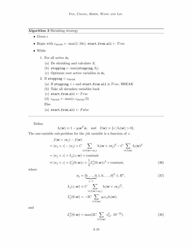
Algorithm 3 Shrinking strategy

• Given ε

• Begin with εshrink ← max(1, 10ε), start from all← True

• While

1. For all active αi

(a) Do shrinking and calculate Si

(b) stopping← max(stopping, Si)

(c) Optimize over active variables in αi

2. If stopping < εshrink

(a) If stopping < ε and start from all is True, BREAK

(b) Take all shrunken variables back

(c) start from all← True

(d) εshrink ← max(ε, εshrink/2)

Else

(a) start from all← False

Definebi(w) ≡ 1− yiwTxi and I(w) ≡ {i | bi(w) > 0}.

The one-variable sub-problem for the jth variable is a function of z:

f(w + zej)− f(w)

= |wj + z| − |wj |+ C∑

i∈I(w+zej)

bi(w + zej)2 − C

∑i∈I(w)

bi(w)2

= |wj + z|+ Lj(z;w) + constant

≈ |wj + z|+ L′j(0;w)z +1

2L′′j (0;w)z2 + constant, (36)

where

ej = [0, . . . , 0︸ ︷︷ ︸j−1

, 1, 0, . . . , 0]T ∈ Rn, (37)

Lj(z;w) ≡ C∑

i∈I(w+zej)

bi(w + zej)2,

L′j(0;w) = −2C∑i∈I(w)

yixijbi(w),

and

L′′j (0;w) = max(2C∑i∈I(w)

x2ij , 10−12). (38)

A.10

LIBLINEAR: A Library for Large Linear Classification

Note that Lj(z;w) is differentiable but not twice differentiable, so 2C∑

i∈I(w) x2ij in (38)

is a generalized second derivative (Chang et al., 2008) at z = 0. This value may be zeroif xij = 0, ∀i ∈ I(w), so we further make it strictly positive. The Newton direction fromminimizing (36) is

d =

−L′j(0;w)+1

L′′j (0;w)if L′j(0;w) + 1 ≤ L′′j (0;w)wj ,

−L′j(0;w)−1

L′′j (0;w)if L′j(0;w)− 1 ≥ L′′j (0;w)wj ,

−wj otherwise.

See the derivation in (Yuan et al., 2010, Appendix B). We then conduct a line searchprocedure to check if d, βd, β2d, . . . , satisfy the following sufficient decrease condition:

|wj + βtd| − |wj |+ C∑

i∈I(w+βtdej)

bi(w + βtdej)2 − C

∑i∈I(w)

bi(w)2

≤ σβt(L′j(0;w)d+ |wj + d| − |wj |

),

(39)

where t = 0, 1, 2, . . . , β ∈ (0, 1), and σ ∈ (0, 1). From Chang et al. (2008, Lemma 5),

C∑

i∈I(w+dej)

bi(w + dej)2 − C

∑i∈I(w)

bi(w)2 ≤ C(

l∑i=1

x2ij)d

2 + L′j(0;w)d.

We can precompute∑l

i=1 x2ij and check

|wj + βtd| − |wj |+ C(

l∑i=1

x2ij)(β

td)2 + L′j(0;w)βtd

≤ σβt(L′j(0;w)d+ |wj + d| − |wj |

),

(40)

before (39). Note that checking (40) is very cheap. The main cost in checking (39) is oncalculating bi(w + βtdej), ∀i. To save the number of operations, if bi(w) is available, onecan use

bi(w + βtdej) = bi(w)− (βtd)yixij . (41)

Therefore, we store and maintain bi(w) in an array. Since bi(w) is used in every linesearch step, we cannot override its contents. After the line search procedure, we mustrun (41) again to update bi(w). That is, the same operation (41) is run twice, where thefirst is for checking the sufficient decrease condition and the second is for updating bi(w).Alternatively, one can use another array to store bi(w+βtdej) and copy its contents to thearray for bi(w) in the end of the line search procedure. We propose the following trick touse only one array and avoid the duplicated computation of (41). From

bi(w + dej) = bi(w)− dyixij ,bi(w + βdej) = bi(w + dej) + (d− βd)yixij ,

bi(w + β2dej) = bi(w + βdej) + (βd− β2d)yixij ,

...

(42)

A.11

Fan, Chang, Hsieh, Wang and Lin

at each line search step, we obtain bi(w+βtdej) from bi(w+βt−1dej) in order to check thesufficient decrease condition (39). If the condition is satisfied, then the bi array already hasvalues needed for the next sub-problem. If the condition is not satisfied, using bi(w+βtdej)on the right-hand side of the equality (42), we can obtain bi(w+ βt+1dej) for the next linesearch step. Therefore, we can simultaneously check the sufficient decrease condition andupdate the bi array. A summary of the procedure is in Algorithm 4.

The stopping condition is by checking the optimality condition. An optimal wj satisfiesL′j(0;w) + 1 = 0 if wj > 0,

L′j(0;w)− 1 = 0 if wj < 0,

−1 ≤ L′j(0;w) ≤ 1 if wj = 0.

(43)

We calculate

vj ≡

|L′j(0;w) + 1| if wj > 0,

|L′j(0;w)− 1| if wj < 0,

max(L′j(0;w)− 1, −1− L′j(0;w), 0

)if wj = 0,

to measure how the optimality condition is violated. The procedure stops if

n∑j=1

(vj at the current iteration)

≤ 0.01× min(#pos,#neg)

l×

n∑j=1

(vj at the 1st iteration) ,

where #pos and #neg indicate the numbers of positive and negative labels in a data set,respectively.

Due to the sparsity of the optimal solution, some wj become zeros in the middle ofthe optimization procedure and are not changed subsequently. We can shrink these wjcomponents to reduce the number of variables. From (43), an optimal wj satisfies that

−1 < L′j(0;w) < 1 implies wj = 0.

If at one iteration, wj = 0 and

−1 +M ≤ L′j(0;w) ≤ 1−M,

where

M ≡ maxj (vj at the previous iteration)

l,

we conjecture that wj will not be changed in subsequent iterations. We then remove thiswj from the optimization problem.

A.12

LIBLINEAR: A Library for Large Linear Classification

Appendix G. L1-regularized Logistic Regression

In LIBLINEAR (after version 1.8), we implement an improved GLMNET, called newGLMNET,for solving L1-regularized logistic regression. GLMNET was proposed by Friedman et al.(2010), while details of newGLMNET can be found in Yuan et al. (2012). Here, we provideimplementation details not mentioned in Yuan et al. (2012).

The problem formulation is in (6). To avoid handling yi in e−yiwTxi , we reformulate

f(w) as

f(w) = ‖w‖1 + C

l∑i=1

log(1 + e−wTxi) +

∑i:yi=−1

wTxi

.

We define

L(w) ≡ C

l∑i=1

log(1 + e−wTxi) +

∑i:yi=−1

wTxi

.

The gradient and Hessian of ∇L(w) can be written as

∇jL(w) = C

l∑i=1

−xij1 + ewTxi

+∑

i:yi=−1

xij

, and

∇2jjL(w) = C

(l∑

i=1

(xij

1 + ewTxi

)2

ewTxi

).

(44)

For line search, we use the following form of the sufficient decrease condition:

f(w + βtd)− f(w)

= ‖w + βtd‖1 − ‖w‖1 + C

l∑i=1

log

(1 + e−(w+βtd)Txi

1 + e−wTxi

)+ βt

∑i:yi=−1

dTxi

= ‖w + βtd‖1 − ‖w‖1 + C

l∑i=1

log

(e(w+βtd)Txi + 1

e(w+βtd)Txi + eβtdTxi

)+ βt

∑i:yi=−1

dTxi

≤ σβt

(∇L(w)Td+ ‖w + d‖1 − ‖w‖1

), (45)

where d is the search direction, β ∈ (0, 1) and σ ∈ (0, 1). From (44) and (45), all we need

is to maintain dTxi and ewTxi ,∀i. We update ew

Txi by

e(w+λd)Txi = ewTxi · eλdTxi , ∀i.

Appendix H. Implementation of L1-regularized Logistic Regression inLIBLINEAR Versions 1.4–1.7

In the earlier versions of LIBLINEAR (versions 1.4–1.7), a coordinate descent method isimplemented for L1-regularized logistic regression. It is similar to the method for L1-regularized L2-loss SVM in Appendix F.

A.13

Fan, Chang, Hsieh, Wang and Lin

The problem formulation is in (6). To avoid handling yi in e−yiwTxi , we reformulate

f(w) as

f(w) = ‖w‖1 + C

l∑i=1

log(1 + e−wTxi) +

∑i:yi=−1

wTxi

.

At each iteration, we select an index j and minimize the following one-variable function ofz:

f(w + zej)− f(w)

= |wj + z| − |wj |+ C

l∑i=1

log(1 + e−(w+zej)Txi) +∑

i:yi=−1

(w + zej)Txi

− C

l∑i=1

log(1 + e−wTxi) +

∑i:yi=−1

wTxi

= |wj + z|+ Lj(z;w) + constant

≈ |wj + z|+ L′j(0;w)z +1

2L′′j (0;w)z2 + constant, (46)

where ej is defined in (37),

Lj(z;w) ≡ C

l∑i=1

log(1 + e−(w+zej)Txi) +∑

i:yi=−1

(w + zej)Txi

,

L′j(0;w) = C

l∑i=1

−xijewTxi + 1

+∑

i:yi=−1

xij

, and

L′′j (0;w) = C

(l∑

i=1

(xij

ewTxi + 1

)2

ewTxi

).

The optimal solution d of minimizing (46) is:

d =

−L′j(0;w)+1

L′′j (0;w)if L′j(0;w) + 1 ≤ L′′j (0;w)wj ,

−L′j(0;w)−1

L′′j (0;w)if L′j(0;w)− 1 ≥ L′′j (0;w)wj ,

−wj otherwise.

A.14

LIBLINEAR: A Library for Large Linear Classification

We then conduct a line search procedure to check if d, βd, β2d, . . . , satisfy the followingsufficient decrease condition:

f(w + βtdej)− f(w)

= C

∑i:xij 6=0

log

(1 + e−(w+βtdej)Txi

1 + e−wTxi

)+ βtd

∑i:yi=−1

xij

+ |wj + βtd| − |wj |

=l∑

i:xij 6=0

C log

(e(w+βtdej)Txi + 1

e(w+βtdej)Txi + eβtdxij

)+ βtd

∑i:yi=−1

Cxij + |wj + βtd| − |wj | (47)

≤ σβt(L′j(0;w)d+ |wj + d| − |wj |

), (48)

where t = 0, 1, 2, . . . , β ∈ (0, 1), and σ ∈ (0, 1).As the computation of (47) is expensive, similar to (40) for L2-loss SVM, we derive an

upper bound for (47). If

x∗j ≡ maxixij ≥ 0,

then

∑i:xij 6=0

C log

(e(w+dej)Txi + 1

e(w+dej)Txi + edxij

)=

∑i:xij 6=0

C log

(ew

Txi + e−dxij

ewTxi + 1

)

≤ (∑

i:xij 6=0

C) log

∑

i:xij 6=0Cew

T xi+e−dxij

ewT xi+1∑

i:xij 6=0C

(49)

= (∑

i:xij 6=0

C) log

1 +

∑i:xij 6=0C

(1

ewT xi+1

(e−dxij − 1))

∑i:xij 6=0C

≤ (∑

i:xij 6=0

C) log

1 +

∑i:xij 6=0C

(1

ewT xi+1

(xije

−dx∗j

x∗j+

x∗j−xijx∗j− 1)

)∑

i:xij 6=0C

(50)

= (∑

i:xij 6=0

C) log

1 +(e−dx

∗j − 1)

∑i:xij 6=0

Cxij

ewT xi+1

x∗j∑

i:xij 6=0C

, (51)

where (49) is from Jensen’s inequality and (50) is from the convexity of the exponentialfunction:

e−dxij ≤ xijx∗je−dx

∗j +

x∗j − xijx∗j

e0 if xij ≥ 0. (52)

As f(w) can also be represented as

f(w) = ‖w‖1 + C

l∑i=1

log(1 + ewTxi)−

∑i:yi=1

wTxi

,

A.15

Fan, Chang, Hsieh, Wang and Lin

we can derive another similar bound∑i:xij 6=0

C log

(1 + e(w+dej)Txi

1 + ewTxi

)

≤ (∑

i:xij 6=0

C) log

1 +(edx

∗j − 1)

∑i:xij 6=0

CxijewT xi

ewT xi+1

x∗j∑

i:xij 6=0C

. (53)

Therefore, before checking the sufficient decrease condition (48), we check if

min((53)− βtd

∑i:yi=1

Cxij + |wj + βtd| − |wj |,

(51) + βtd∑

i:yi=−1

Cxij + |wj + βtd| − |wj |)

≤ σβt(L′j(0;w)d+ |wj + d| − |wj |

).

(54)

Note that checking (54) is very cheap since we already have

∑i:xij 6=0

Cxij

ewTxi + 1and

∑i:xij 6=0

CxijewTxi

ewTxi + 1

in calculating L′j(0;w) and L′′j (0;w). However, to apply (54) we need that the data setsatisfies xij ≥ 0, ∀i,∀j. This condition is used in (52).

The main cost in checking (47) is on calculating e(w+βtdej)Txi , ∀i. To save the number

of operations, if ewTxi is available, one can use

e(w+βtdej)Txi = ewTxie(βtd)xij .

Therefore, we store and maintain ewTxi in an array. The setting is similar to the array

1 − yiwTxi for L2-loss SVM in Appendix F, so one faces the same problem of not beingable to check the sufficient decrease condition (48) and update the ew

Txi array together. Wecan apply the same trick in Appendix F, but the implementation is more complicated. Inour implementation, we allocate another array to store e(w+βtdej)Txi and copy its contentsfor updating the ew

Txi array in the end of the line search procedure. A summary of theprocedure is in Algorithm 5.

The stopping condition and the shrinking implementation to remove some wj compo-nents are similar to those for L2-loss support vector machines (see Appendix F).

Appendix I. L2-regularized Logistic Regression (Solving Dual)

See Yu et al. (2011) for details of a dual coordinate descent method.

Appendix J. L2-regularized Logistic Regression (Solving Dual)

See Yu et al. (2011) for details of a dual coordinate descent method.

A.16

LIBLINEAR: A Library for Large Linear Classification

Appendix K. L2-regularized Support Vector Regression

LIBLINEAR solves both the primal and the dual of L2-loss SVR, but only the dual of L1-lossSVR. The dual SVR is solved by a coordinate descent, and the primal SVR is solved by atrust region Newton method. See Ho and Lin (2012) for details of them. In Appendix C, wementioned that the trust region Newton method is improved in version 2.11 and 2.20 (Seedetails in Hsia et al. (2017b) and Hsia et al. (2017a)). Both modifications are applicable tothe primal SVR solver.

Appendix L. Probability Outputs

Currently we support probability outputs for logistic regression only. Although it is possibleto apply techniques in LIBSVM to obtain probabilities for SVM, we decide not to implementit for code simplicity.

The probability model of logistic regression is

P (y|x) =1

1 + e−ywTx, where y = ±1,

so probabilities for two-class classification are immediately available. For a k-class problem,we need to couple k probabilities

1 vs. not 1: P (y = 1|x) = 1/(1 + e−wT1 x)

...

k vs. not k: P (y = k|x) = 1/(1 + e−wTk x)

together, where w1, . . . ,wk are k model vectors obtained after the one-vs-the-rest strategy.Note that the sum of the above k values is not one. A procedure to couple them can befound in Section 4.1 of Huang et al. (2006), but for simplicity, we implement the followingheuristic:

P (y|x) =1/(1 + e−w

Ty x)∑k

m=1 1/(1 + e−wTmx)

.

Appendix M. Automatic and Efficient Parameter Selection

See Chu et al. (2015) for details of the procedure and Section N.5 for the practical use.

A.17

Fan, Chang, Hsieh, Wang and Lin

Algorithm 4 A coordinate descent algorithm for L1-regularized L2-loss SVC

• Choose β = 0.5 and σ = 0.01. Given initial w ∈ Rn.

• Calculatebi ← 1− yiwTxi, i = 1, . . . , l.

• While w is not optimal

For j = 1, 2, . . . , n

1. Find the Newton direction by solving

minz

|wj + z|+ L′j(0;w)z +1

2L′′j (0;w)z2.

The solution is

d =

−L′j(0;w)+1

L′′j (0;w)if L′j(0;w) + 1 ≤ L′′j (0;w)wj ,

−L′j(0;w)−1

L′′j (0;w)if L′j(0;w)− 1 ≥ L′′j (0;w)wj ,

−wj otherwise.

2. d← 0; ∆← L′j(0;w)d+ |wj + d| − |wj |.3. While t = 0, 1, 2, . . .

(a) If

|wj + d| − |wj |+ C(

l∑i=1

x2ij)d

2 + L′j(0;w)d ≤ σ∆,

thenbi ← bi + (d− d)yixij , ∀i and BREAK.

(b) If t = 0, calculate

Lj,0 ← C∑i∈I(w)

b2i .

(c) bi ← bi + (d− d)yixij , ∀i.(d) If

|wj + d| − |wj |+ C∑

i∈I(w+dej)

b2i − Lj,0 ≤ σ∆,

then

BREAK.

Elsed← d; d← βd; ∆← β∆.

4. Update wj ← wj + d.

A.18

LIBLINEAR: A Library for Large Linear Classification

Algorithm 5 A coordinate descent algorithm for L1-regularized logistic regression

• Choose β = 0.5 and σ = 0.01. Given initial w ∈ Rn.

• Calculatebi ← ew

Txi , i = 1, . . . , l.

• While w is not optimal

For j = 1, 2, . . . , n

1. Find the Newton direction by solving

minz

|wj + z|+ L′j(0;w)z +1

2L′′j (0;w)z2.

The solution is

d =

−L′j(0;w)+1

L′′j (0;w)if L′j(0;w) + 1 ≤ L′′j (0;w)wj ,

−L′j(0;w)−1

L′′j (0;w)if L′j(0;w)− 1 ≥ L′′j (0;w)wj ,

−wj otherwise.

2. ∆← L′j(0;w)d+ |wj + d| − |wj |.3. While

(a) If mini,j xij ≥ 0 and

min((53)− d

∑i:yi=1

Cxij + |wj + d| − |wj |,

(51) + d∑

i:yi=−1

Cxij + |wj + d| − |wj |)

≤ σ∆,

thenbi ← bi × edxij , ∀i and BREAK.

(b) bi ← bi × edxij , ∀i.(c) If

∑i:xij 6=0

C log

(bi + 1

bi + edxij

)+ d

∑i:yi=−1

Cxij + |wj + d| − |wj | ≤ σ∆,

thenbi ← bi, ∀i and BREAK.

Elsed← βd; ∆← β∆.

4. Update wj ← wj + d.

A.19

Fan, Chang, Hsieh, Wang and Lin

A Practical Guide to LIBLINEARAppendix N.

In this section, we present a practical guide for LIBLINEAR users. For instructions of usingLIBLINEAR and additional information, see the README file included in the package and theLIBLINEAR FAQ, respectively.

N.1 When to Use Linear (e.g., LIBLINEAR) Rather Then Nonlinear (e.g.,LIBSVM)?

Please see the discussion in Appendix C of Hsu et al. (2003).

N.2 Data Preparation (In Particular, Document Data)

LIBLINEAR can be applied to general problems, but it is particularly useful for documentdata. We discuss how to transform documents to the input format of LIBLINEAR.

A data instance of a classification problem is often represented in the following form.

label feature 1, feature 2, . . ., feature n

The most popular method to represent a document is the “bag-of-words” model (Harris,1954), which considers each word as a feature. Assume a document contains the followingtwo sentences

This is a simple sentence.This is another sentence.

We can transfer this document to the following Euclidean vector:

a an · · · another · · · is · · · this · · ·1 0 · · · 1 · · · 2 · · · 2 · · ·

The feature “is” has a value 2 because “is” appears twice in the document. This type ofdata often has the following two properties.

1. The number of features is large.

2. Each instance is sparse because most feature values are zero.

Let us consider a 20-class data set news20 at libsvmtools.5 The first instance is

1 197:2 321:3 399:1 561:1 575:1 587:1 917:1 1563:1 1628:3 1893:1 3246:1 4754:2

6053:1 6820:1 6959:1 7571:1 7854:2 8407:1 11271:1 12886:1 13580:1 13588:1

13601:2 13916:1 14413:1 14641:1 15950:1 20506:1 20507:1

Each (index:value) pair indicates a word’s “term frequency” (TF). In practice, additionalsteps such as removing stop words or stemming (i.e., using only root words) may be applied,although we do not discuss details here.

Existing methods to generate document feature vectors include

5. http://www.csie.ntu.edu.tw/~cjlin/libsvmtools/datasets/multiclass.html#news20

A.20

LIBLINEAR: A Library for Large Linear Classification

1. TF: term frequency.

2. TF-IDF (term frequency, inverse document frequency); see Salton and Yang (1973)and any information retrieval book.

3. binary: each feature indicates if a word appears in the document or not.

For example, the binary-feature vector of the news20 instance is

1 197:1 321:3 399:1 561:1 575:1 587:1 917:1 1563:1 1628:3 1893:1 3246:1 4754:1

6053:1 6820:1 6959:1 7571:1 7854:1 8407:1 11271:1 12886:1 13580:1 13588:1

13601:1 13916:1 14413:1 14641:1 15950:1 20506:1 20507:1

Our past experiences indicate that binary and TF-IDF are generally useful if normalizationhas been properly applied (see the next section).

N.3 Normalization

In classification, large values in data may cause the following problems.

1. Features in larger numeric ranges may dominate those in smaller ranges.

2. Optimization methods for training may take longer time.

The typical remedy is to scale data feature-wisely. This is suggested in the popular SVMguide by Hsu et al. (2003).6 However, for document data, often a simple instance-wisenormalization is enough. Each instance becomes a unit vector; see the following normalizednews20 instance.

1 197:0.185695 321:0.185695 399:0.185695 561:0.185695 575:0.185695 587:0.185695

917:0.185695 1563:0.185695 1628:0.185695 1893:0.185695 3246:0.185695 4754:0.185695

6053:0.185695 6820:0.185695 6959:0.185695 7571:0.185695 7854:0.185695 8407:0.185695

11271:0.185695 12886:0.185695 13580:0.185695 13588:0.185695 13601:0.185695

13916:0.185695 14413:0.185695 14641:0.185695 15950:0.185695 20506:0.185695 20507:0.185695

There are 29 non-zero features, so each one has the value 1/√

29. We run LIBLINEAR tofind five-fold cross-validation (CV) accuracy on the news20 data.7 For the original datausing TF features, we have

$ time ./train -v 5 news20

Cross Validation Accuracy = 80.4644%

57.527s

During the computation, the following warning message appears many times to indicatecertain difficulties.

WARNING: reaching max number of iterations

6. For sparse data, scaling each feature to [0, 1] is more suitable than [−1, 1] because the latter makes theproblem has many non-zero elements.

7. Experiments in this guide were run on a 64-bit machine with Intel Xeon 2.40GHz CPU (E5530), 8MBcache, and 72GB main memory.

A.21

Fan, Chang, Hsieh, Wang and Lin

Table 1: Current solvers in LIBLINEAR for L2-regularized problems.

Dual-based solvers (coordinate de-scent methods)

Primal-based solvers (Newton-type methods)

Property Extremely fast in some situations,but may be very slow in some oth-ers

Moderately fast in most situa-tions

When to useit

1. Large sparse data (e.g., docu-ments) under suitable scaling and Cis not too large2. Data with # instances � # fea-tures

Others

If data is transformed to binary and then normalized, we have

$ time ./train -v 5 news20.scale

Cross Validation Accuracy = 84.7254%

6.140s

Clearly, the running time for the normalized data is much shorter and no warning messageappears.

Another example is in Lewis et al. (2004), which normalizes each log-transformed TF-IDF feature vector to have unit length.

N.4 Selection of Solvers

Appendix A lists many LIBLINEAR’s solvers. Users may wonder how to choose them.Fortunately, these solvers usually give similar performances. Some in fact generate thesame model because they differ in only solving the primal or dual optimization problems.For example, -s 1 solves dual L2-regularized L2-loss SVM, while -s 2 solves primal.

$ ./train -s 1 -e 0.0001 news20.scale

(skipped)

Objective value = -576.922572

nSV = 3540

$./train -s 2 -e 0.0001 news20.scale

(skipped)

iter 7 act 1.489e-02 pre 1.489e-02 delta 1.133e+01 f 5.769e+02 |g| 3.798e-01 CG 10

Each run trains 20 two-class models, so we only show objective values of the last one.Clearly, the dual objective value -576.922572 coincides with the primal value 5.769e+02.We use the option -e to impose a smaller stopping tolerance, so optimization problems aresolved more accurately.

While LIBLINEAR’s solvers give similar performances, their training time may be differ-ent. For current solvers for L2-regularized problems, a rough guideline is in Table 1. Werecommend users

A.22

LIBLINEAR: A Library for Large Linear Classification

1. Try the default dual-based solver first.

2. If it is slow, check primal-based solvers.

For L1-regularized problems, the choice is limited because currently we only offer primal-based solvers.

To choose between using L1 and L2 regularization, we recommend trying L2 first unlessusers need a sparse model. In most cases, L1 regularization does not give higher accuracybut may be slightly slower in training; see a comparison in Section D of the supplemenarymaterials of Yuan et al. (2010).

N.5 Parameter Selection

For linear classification, the only parameter is C in Eq. (1). We summarize some propertiesbelow.

1. Solvers in LIBLINEAR is not very sensitive to C. Once C is larger than certain value,the obtained models have similar performances. A theoretical proof of this kind ofresults is in Theorem 3 of Keerthi and Lin (2003).

2. Using a larger C value usually causes longer training time. Users should avoid tryingsuch values.

We conduct the following experiments to illustrate these properties. To begin, we show inFigure 2 the relationship between C and CV accuracy. Clearly, CV rates are similar afterC is large enough. For running time, we compare the results using C = 1 and C = 100.

$ time ./train -c 1 news20.scale

2.528s

$ time ./train -c 100 news20.scale

28.589s

We can see that a larger C leads to longer training time. Here a dual-based coordinatedescent method is used. For primal-based solvers using Newton methods, the running timeis usually less affected by the change of C.

$ time ./train -c 1 -s 2 news20.scale

8.596s

$ time ./train -c 100 -s 2 news20.scale

11.088s

While users can try a few C values by themselves, LIBLINEAR (after version 2.0) providesan easy solution to find a suitable parameter. If primal-based classification solvers are used(-s 0 or -s 2), the -C option efficiently conducts cross validation several times and findsthe best parameter automatically.

$ ./train -C -s 2 news20.scale

log2c= -15.00 rate=69.0806

log2c= -14.00 rate=69.3505

A.23

Fan, Chang, Hsieh, Wang and Lin

log2C

CV

-14 -10 -6 -2 2 6 10 14

70

75

80

85

Figure 2: CV accuracy versus log2C.

(skipped)

log2c= 9.00 rate=83.7151

log2c= 10.00 rate=83.6837

warning: maximum C reached.

Best C = 1.000000 CV accuracy = 84.7192%

Users do not need to specify the range of C to explore because LIBLINEAR finds a reasonablerange automatically. Note that users can still use the -c option to specify the smallest Cvalue of the search range. For example,

$ ./train -C -s 2 -c 0.5 -e 0.0001 news20.scale

log2c= -1.00 rate=84.5623

log2c= 0.00 rate=84.7254

(skipped)

log2c= 9.00 rate=83.6272

log2c= 10.00 rate=83.621

warning: maximum C reached.

Best C = 1.000000 CV accuracy = 84.7254%

This option is useful when users want to rerun the parameter selection procedure from aspecified C under a different setting, such as a stricter stopping tolerance -e 0.0001 in theabove example.

Note that after finding the best C, users must apply the same solver to train a modelfor future prediction. Switching from a primal-based solver to a corresponding dual-basedsolver (e.g., from -s 2 to -s 1) is fine because they produce the same model.

Some solvers such as -s 5 or -s 6 are not covered by the -C option.8 We can use aparameter selection tool grid.py in LIBSVM to find the best C value. For example,

$ ./grid.py -log2c -14,14,1 -log2g null -svmtrain ./train -s 5 news20.scale

8. Note that we have explained that for some dual-based solvers you can use -C on their correspondingprimal-based solvers for parameter selection.

A.24

LIBLINEAR: A Library for Large Linear Classification

checks the CV rates of C ∈ {2−14, 2−13, . . . , 214}. Note that grid.py should be used onlyif -C is not available for the desired solver. The -C option is much faster than grid.py ona single computer.

References

Kai-Wei Chang, Cho-Jui Hsieh, and Chih-Jen Lin. Coordinate descent method for large-scale L2-loss linear SVM. Journal of Machine Learning Research, 9:1369–1398, 2008.URL http://www.csie.ntu.edu.tw/~cjlin/papers/cdl2.pdf.

Bo-Yu Chu, Chia-Hua Ho, Cheng-Hao Tsai, Chieh-Yen Lin, and Chih-Jen Lin. Warm startfor parameter selection of linear classifiers. In Proceedings of the 21th ACM SIGKDDInternational Conference on Knowledge Discovery and Data Mining (KDD), 2015. URLhttp://www.csie.ntu.edu.tw/~cjlin/libsvmtools/warm-start/warm-start.pdf.

Koby Crammer and Yoram Singer. On the learnability and design of output codes formulticlass problems. In Computational Learning Theory, pages 35–46, 2000.

Jerome H. Friedman, Trevor Hastie, and Robert Tibshirani. Regularization paths for gen-eralized linear models via coordinate descent. Journal of Statistical Software, 33(1):1–22,2010.

Zellig S. Harris. Distributional structure. Word, 10:146–162, 1954.

Chia-Hua Ho and Chih-Jen Lin. Large-scale linear support vector regression. Journal ofMachine Learning Research, 13:3323–3348, 2012. URL http://www.csie.ntu.edu.tw/

~cjlin/papers/linear-svr.pdf.

Chih-Yang Hsia, Wei-Lin Chiang, and Chih-Jen Lin. Preconditioned conjugate gradientmethods in truncated Newton frameworks for large-scale linear classification. Technicalreport, Department of Computer Science, National Taiwan University, 2017a.

Chih-Yang Hsia, Ya Zhu, and Chih-Jen Lin. A study on trust region update rules in New-ton methods for large-scale linear classification. In Proceedings of the Asian Conferenceon Machine Learning (ACML), 2017b. URL http://www.csie.ntu.edu.tw/~cjlin/

papers/newtron/newtron.pdf.

Cho-Jui Hsieh, Kai-Wei Chang, Chih-Jen Lin, S. Sathiya Keerthi, and Sellamanickam Sun-dararajan. A dual coordinate descent method for large-scale linear SVM. In Proceedingsof the Twenty Fifth International Conference on Machine Learning (ICML), 2008. URLhttp://www.csie.ntu.edu.tw/~cjlin/papers/cddual.pdf.

Chih-Wei Hsu, Chih-Chung Chang, and Chih-Jen Lin. A practical guide to support vectorclassification. Technical report, Department of Computer Science, National Taiwan Uni-versity, 2003. URL http://www.csie.ntu.edu.tw/~cjlin/papers/guide/guide.pdf.

Tzu-Kuo Huang, Ruby C. Weng, and Chih-Jen Lin. Generalized Bradley-Terry models andmulti-class probability estimates. Journal of Machine Learning Research, 7:85–115, 2006.URL http://www.csie.ntu.edu.tw/~cjlin/papers/generalBT.pdf.

A.25

Fan, Chang, Hsieh, Wang and Lin

S. Sathiya Keerthi and Chih-Jen Lin. Asymptotic behaviors of support vector machineswith Gaussian kernel. Neural Computation, 15(7):1667–1689, 2003.

S. Sathiya Keerthi, Sellamanickam Sundararajan, Kai-Wei Chang, Cho-Jui Hsieh, and Chih-Jen Lin. A sequential dual method for large scale multi-class linear SVMs. In Proceed-ings of the Forteenth ACM SIGKDD International Conference on Knowledge Discoveryand Data Mining, pages 408–416, 2008. URL http://www.csie.ntu.edu.tw/~cjlin/

papers/sdm_kdd.pdf.

Ching-Pei Lee and Chih-Jen Lin. A study on L2-loss (squared hinge-loss) multi-classSVM. Neural Computation, 25(5):1302–1323, 2013. URL http://www.csie.ntu.edu.

tw/~cjlin/papers/l2mcsvm/l2mcsvm.pdf.

David D. Lewis, Yiming Yang, Tony G. Rose, and Fan Li. RCV1: A new benchmarkcollection for text categorization research. Journal of Machine Learning Research, 5:361–397, 2004.

Chih-Jen Lin, Ruby C. Weng, and S. Sathiya Keerthi. Trust region Newton method forlarge-scale logistic regression. Journal of Machine Learning Research, 9:627–650, 2008.URL http://www.csie.ntu.edu.tw/~cjlin/papers/logistic.pdf.

Gerard Salton and Chung-Shu Yang. On the specification of term values in automaticindexing. Journal of Documentation, 29:351–372, 1973.

Paul Tseng and Sangwoon Yun. A coordinate gradient descent method for nonsmoothseparable minimization. Mathematical Programming, 117:387–423, 2009.

Hsiang-Fu Yu, Fang-Lan Huang, and Chih-Jen Lin. Dual coordinate descent methodsfor logistic regression and maximum entropy models. Machine Learning, 85(1-2):41–75,October 2011. URL http://www.csie.ntu.edu.tw/~cjlin/papers/maxent_dual.pdf.

Guo-Xun Yuan, Kai-Wei Chang, Cho-Jui Hsieh, and Chih-Jen Lin. A comparison of opti-mization methods and software for large-scale l1-regularized linear classification. Journalof Machine Learning Research, 11:3183–3234, 2010. URL http://www.csie.ntu.edu.

tw/~cjlin/papers/l1.pdf.

Guo-Xun Yuan, Chia-Hua Ho, and Chih-Jen Lin. An improved GLMNET for l1-regularizedlogistic regression. Journal of Machine Learning Research, 13:1999–2030, 2012. URLhttp://www.csie.ntu.edu.tw/~cjlin/papers/l1_glmnet/long-glmnet.pdf.

A.26