Leverage effects and stochastic volatility in spot oil returns: A

Bayesian approach with VaR and CVaR applications†

Liyuan Chena,∗, Paola Zerillia, Christopher F. Baumb,c

aDepartment of Economics and Related Studies, University of York, United KingdombDepartment of Economics, Boston College, USA

cDepartment of Macroeconomics, German Institute for Economic Research (DIW Berlin), Germany

Abstract

Crude oil markets have been quite volatile and risky in the past few decades due to the large

fluctuations of oil prices. We contribute to the current debate by testing for the existence of

the leverage effect when considering daily spot returns in the WTI and Brent crude oil markets

and by studying the direct impact of the leverage effect on measures of risk such as VaR and

CVaR. More specifically, we model spot crude oil returns using Stochastic Volatility (SV)

models with various distributions of the errors. We find that the introduction of the leverage

effect in the traditional SV model with Normally distributed errors is capable of adequately

estimating risk for conservative oil suppliers in both the WTI and Brent markets while it

tends to overestimate risk for more speculative oil suppliers. Our results also show that

the choice of financial regulators, both on the supply and on the demand side, would not be

affected by the introduction of leverage. Focusing instead on firm’s internal risk management,

our results show that the introduction of leverage would be useful for firms who are on the

demand side for oil, who use VaR for risk management and who are particularly worried

about the magnitude of the losses exceeding VaR while wanting to minimize the opportunity

cost of capital. Using the same logic, firms who are on the supply side, would be better off

not considering the leverage effect.

Keywords: Value-at-Risk, Conditional Value-at-Risk, Asymmetric Laplace distribution,

Stochastic volatility model, Bayesian Markov Chain Monte Carlo, leverage effect

JEL Classifications: C11, C58, G17, G32

∗Corresponding author. Department of Economics and Related Studies, University of York, Heslington,York YO10 5DD, United Kingdom. Tel.: +44 7541766512

Email addresses: lc844@york.ac.uk (Liyuan Chen), paola.zerilli@york.ac.uk (Paola Zerilli),kit.baum@bc.edu (Christopher F. Baum)

† We thank Carlos Antonio Abanto-Valle, Giacomo Bormetti, Richard Gerlach, Jouchi Nakajima, SjurWestgaard, Nuttanan Wichitaksorn and two anonymous referees for helpful comments and suggestions.This paper also benefited from comments by seminar participants at the 5th Asian Quantitative FinanceConference, the 24th International Conference on Forecasting Financial Markets, 2017 InternationalConference on Energy Finance and the 17th China Economics Annual Conference.

Preprint submitted to Energy Economics January 28, 2018

1. Introduction

Crude oil markets have been quite volatile and risky in the past few decades due to the

large fluctuations of oil prices. This has become a principal concern for oil suppliers, oil

consumers, relevant firms and governments. In addition, as a primary source of energy in the

power industry, industrial production and transportation, volatile oil prices may lead to cost

uncertainties for other markets, thus extensively affecting the development of the economy.

A large number of studies have shown that oil price fluctuations could have considerable

impact on economic activities. Papapetrou (2001) argues that the variability of oil prices

plays a critical role in affecting real economic activity and employment. Lardic and Mignon

(2008) explore the long-term relationship between oil prices and GDP, and find evidence that

aggregate economic activity seems to slow down particularly when oil prices increase. This

asymmetry is found in both the U.S. and European countries. Consequently, quantifying

and managing the risks inherent to the volatility of oil prices has become critical for both

researchers and energy market participants.

The Value at Risk (VaR) measure, which was first proposed by J.P. Morgan in the

RiskMetrics model in 1994, has been developed as one of the most popular approaches

in financial markets to manage market risk. VaR defines the maximum amount that an

investor can face for a given tolerance level over a certain time horizon. Although VaR is

recommended by Basel II and III and has been widely adopted by financial institutions, it

has been challenged by the Bank of International Settlements (BIS) Committee, who pointed

out that VaR cannot measure market risk as it fails to consider the extreme tail events of

a return distribution (see, Chen et al., 2012). In addition, Artzner et al. (1999) argue that

VaR does not meet the requirements of sub-additivity and thus is not a coherent measure

of risk. As an alternative, they proposed a conservative, but more coherent measure, called

Conditional VaR at risk (CVaR) or expected shortfall (ES), which considers the average loss

as that exceeding the VaR threshold. Given all these factors, in this paper, both measures

are used to quantify financial risks affecting oil markets. Existing literature that uses VaR

and CVaR to measure these risks generally focuses on the scenario of a declining oil price

(i.e. downside risk). However, the oil market has its own traits which are quite different from

those of financial assets. More specifically, when oil prices fall due to sudden negative news,

countries exporting oil or oil producers would inevitably incur losses while oil consumers

would benefit from those negative extreme events. On the other hand, if oil prices rise

suddenly, oil consumers would suffer a financial loss. Therefore, in this paper we consider

risks affecting both oil supply and oil demand.

In recent years, the commodity price literature has shown that there is evidence of

leverage effects in various energy markets. More specifically, Chan and Grant (2016a),

considering lower frequency (weekly) commodity returns conclude that SV models (with

2

an MA component) are able to replicate the main features of the data more efficiently

than GARCH models. At the same time, they find a significant negative leverage effect

in crude oil spot markets. Kristoufek (2014) focuses on the leverage effect in commodity

futures markets and provides an extensive literature review in this area. Fan et al. (2008)

estimate VaR of crude oil prices using a GED-GARCH approach with daily WTI and Brent

prices spanning from 1987 to 2006. They find that this type of model specification does

as well as the standard normal distribution at a 95% confidence level. They also test and

find evidence for asymmetric leverage effects without modelling them directly. Youssef et

al. (2015) evaluate VaR and CVar for crude oil and gasoline markets using a long memory

GARCH-EVT approach. Their findings and backtesting exercise show that crude oil markets

are characterized by asymmetry, fat tails and long range memory.

We contribute to the current debate by testing for the existence of the leverage effect

when considering daily spot returns in the WTI and Brent crude oil markets and by studying

the direct impact of the leverage effect on measures of risk such as VaR and CVaR. More

specifically, in order to address the risk faced by oil suppliers and oil consumers we model

spot crude oil returns using Stochastic Volatility (SV) models with various distributions of

the errors. Among other cases, we test the assumption of Asymmetric Laplace Distributed

(ALD) errors in order to more carefully model the type of risk faced by oil suppliers versus

the risk faced by oil buyers.

We find that the introduction of the leverage effect in the traditional SV model with

Normally distributed errors is capable of adequately estimating risk (in a VaR and CVaR

sense) for conservative (i.e. more risk averse, with α = 5%) oil suppliers in both the WTI

and Brent markets while it tends to overestimate risk for more speculative oil suppliers

(α = 1%). In comparison, the assumption of ALD errors leads to overestimating risk for both

types of investors. In the model efficiency selection stage, our results show that the choice

of financial regulators, both on the supply and on the demand side, would not be affected

by the introduction of leverage. Focusing instead on firm’s internal risk management, our

results show that the introduction of leverage (SV-N-L model) would be useful for firms who

are on the demand side for oil (in both the WTI and Brent markets), who use VaR for risk

management and who are particularly worried about the magnitude of the losses exceeding

VaR while wanting to minimize the opportunity cost of capital. Using the same logic, firms

who are on the supply side, would be better off not considering the leverage effect (SV-N

model).

3

2. Stochastic volatility models

We use a general SV model to capture the volatility features for oil markets which has

been studied recently by Takahashi et al. (2009), Chai et al. (2011) and Chan et al. (2016a):

yt = µ+ σtzt (1)

lnσ2t = ht = δ + β(lnσ2

t−1 − δ) + ηt ηt ∼ N(0, σ2η) (2)

where yt denotes stock returns at time t with t = 1, 2, ..., T , µ denotes the conditional mean, σt

is the stochastic volatility, lnσ2t follows a stationary AR(1) process with persistence parameter

β having |β| < 1, zt and ηt represent a series of independent identical (i.i.d.) random errors

in the return and volatility equation, respectively.2

For this general equation, we consider various possible specifications of the shocks zt

affecting stock returns.

(1) Standard Student t errors

zt ∼ tν

where ν is the degrees of freedom of t-distribution.

(2) Standard Normal errors

zt ∼ N (0, 1)

(3) Standard Asymmetric Laplace errors

zt ∼ ALD (0, κ, 1)

where σ = 1 and κ is the coefficient driving the skewness of the distribution, is related to µ

and σ as follows:

µ =σ√2

(1

κ− κ)

as a special case κ = 1 for µ ' 0 and σ = eht2 > 0 (Symmetric Laplace Distribution).3

2A number of original empirical works via extended SV models can be found from Breidt et al. (1998), Soet al. (1998), Yu and Yang (2002), Koopman and Uspensky (2002), Cappuccio et al. (2004), Chan (2013),Chan and Hsiao (2013), Chan and Grant (2016c), Chan (2017).

3See appendix for the density of ALD.

4

(4) Standard Student t errors with leverage effect

yt = µ+ σtzt

zt ∼ tν

lnσ2t = ht = δ + β

(lnσ2

t−1 − δ)

+ ξt

ξt = ρzt +√

1− ρ2ηt

ηt ∼ N(0, σ2

η

)where the coefficient ρ drives the so called leverage effect. It models the correlation between

the shocks affecting returns and the shocks affecting volatility. For example, a negative ρ

would mean that negative shocks to returns are likely to be associated to positive shocks to

volatility: negative shocks to financial markets would trigger higher volatility and riskiness.

Of course for ρ = 0, the model would be simply the regular SV-t model with no leverage effect.

(5) Standard Normal errors with leverage effect

yt = µ+ σtzt

zt ∼ N (0, 1)

lnσ2t = ht = δ + β

(lnσ2

t−1 − δ)

+ ξt

ξt = ρzt +√

1− ρ2ηt

ηt ∼ N(0, σ2

η

)where ρ is the coefficient driving the leverage effect in the SV-N-L model.

(6) Standard Asymmetric Laplace distributed errors with leverage effect

yt = µ+ σtzt

zt ∼ ALD (0, κ, 1)

lnσ2t = ht = δ + β

(lnσ2

t−1 − δ)

+ ξt

ξt = ρzt +√

1− ρ2ηt

ηt ∼ N(0, σ2

η

)where ρ is the coefficient driving the leverage effect in the SV-ALD-L model.

5

3. VaR and CVaR models

Considering V aRs,t(l) and V aRd,t(l) as the VaR for oil supply and demand in l-period

with confidence level (1− α) ∈ (0, 1) respectively, then, we have:

Supply : Prob (yt(l) ≤ −V aRs,t(l)|Ωt) = α (3)

Demand : Prob (yt(l) ≥ V aRd,t(l)|Ωt) = α (4)

where yt(l) represents the oil return series for period (from t to t+ l), Ωt is the information

set up to time t, α is the risk level, and the value of V aRs,t and V aRd,t are defined to be

positive. Likewise, CV aRs,t(l) and CV aRd,t(l) are defined as the CVaR of oil supply and

demand respectively over period l at confidence level (1−α), and they can be mathematically

expressed as:

Supply : CV aRs,t(l) = −Eyt(l)|yt(l) ≤ −V aRs,t(l) (5)

Demand : CV aRd,t(l) = Eyt(l)|yt(l) ≥ V aRd,t(l) (6)

3.1. In the SV-N setting

Now we introduce the VaR and CVaR formulas under the SV-N framework.

Risk for oil Supply

(1) VaR: V aRn,s,t = −µ− σtΦ−1(α)

where Φ−1(α) is the inverse cumulative distribution function of a N(0,1). In order to model

the leverage effect in this setting, we use σt(ρ).

(2) CVaR: CV aRn,s,t = −E[yt| yt ≤ −V aRn,s,t

]= −µ− σt

αφ(Φ−1(α))

where φ(α) is the probability density function of a N (0,1). To model the leverage effect in

this setting, we use σt(ρ).

Risk for oil demand

(1) VaR: V aRn,d,t = µ+ σtΦ−1(α)

where Φ−1(α) is the inverse cumulative distribution function of a N(0,1). To model the

leverage effect in this setting, we use σt(ρ).

(2) CVaR: CV aRn,d,t = E[yt| yt ≥ V aR

n,d,t

]= µ+

σtαφ(Φ−1(α))

6

where φ(α) is the probability density function of a N (0,1). To model the leverage effect in

this setting, we use σt(ρ).

3.2. In the SV-ALD setting

We now introduce the VaR and CVaR formulas under the SV-ALD model.

Risk for oil Supply

(1) VaR: V aRs,t = −µ+ms,qσt = −µ− κσt√2lnα(1 + κ2)

κ2

where ms,q = (V aRs,t + µ)/σt is defined as the left α-quantile of the AL distribution. In

order to model the leverage effect in this setting, we use σt(ρ).

(2) CVaR: CV aRs,t = −E[yt| yt ≤ −V aRs,t

]= V aRs,t +

κσt√2

To model the leverage effect in this setting, we use σt(ρ).

Risk for oil Demand

(1) VaR: V aRd,t = µ+md,qσt = µ− σt√2κ

ln(α(1 + κ2))

where md,q = (V aRd,t − µ)/σt is the right α-quantile of the AL distribution. To model the

leverage effect in this setting, we use σt(ρ).

(2) CVaR: CV aRd,t = E[yt| yt ≥ V aR

d,t

]= V aRd,t +

σt√2κ

To model the leverage effect in this setting, we use σt(ρ).4

4. Estimation methodology of Bayesian MCMC

In order to improve the tractability of the ALD model, we introduce a modified Bayesian

MCMC method. That is, a new Scale Mixture of Uniform (SMU) representation for the AL

density (following Kotz et al., 2001) is proposed to facilitate the estimation of the SV-ALD

model.

4See appendix B for the derivations of V aRs,t, V aRd,t, CV aRs,t and CV aRd,t.

7

4.1. Scale mixture of uniform representation of ALD

Expressing the ALD via the representation can alleviate the computational burden when

using the Gibbs sampling algorithm in the MCMC approach and thus can simplify the

estimation method in Bayesian analysis. To estimate the latent variables in the SV model,

we use the scaled ALD (SALD) which means that the ALD random variable is scaled by its

standard deviation (See Chen et al., 2009 and Wichitaksorn et al., 2015).

Proposition 1. Let zt be the ALD random variable with zt ∼ ALD(0, κ, 1), then the random

variable εt = ztS.D.[z]

has SALD with p.d.f. given by:

f(εt|κ, σt) =

√

1 + κ4

1 + κ2

1

σtexp(−√

1 + κ4

σtεt) εt ≥ 0

√1 + κ4

1 + κ2

1

σtexp(

√1 + κ4

κ2σtεt) εt < 0

(7)

where κ is skewness parameter and σt is the standard deviation (or the time-varying volatility)

of zt.5

Hence, the corresponding SMU of SALD can be obtained as follows:

Proposition 2. If λt ∼ Ga(2, 1) and εt ∼ U(εt| − λtκ2σt√1+κ4

,+ λtσt√1+κ4

), then the SMU density:

f(εt|κ, λt, σt) =

∫ ∞0

fU(εt| −λtκ

2σt√1 + κ4

,+λtσt√1 + κ4

)× fGa(λt|2, 1) dλt (8)

has the same form as the SALD density function given in equation (7).6

Using the SMU representation of SALD, an efficient simulation algorithm is developed to

overcome parameter estimation difficulties. As a result, the SV model discussed in section 2

can be written hierarchically as:

Return equation:

yt|κ, λt, ht ∼ U(− λtκ2eht/2√

1 + κ4,+

λteht/2

√1 + κ4

) (9)

λt ∼ Ga(2, 1) (10)

5Note that original scale parameter has been canceled in this derivation, while the location parameter θis set to be 0 in real practice. See appendix C for the derivation.

6See appendix D for the derivation.

8

Volatility equation:

ht|δ, β, σ2η, ht−1 ∼N(δ + β(ht−1 − δ), σ2

η) t = 1, 2, ..., T (11)

h1|δ, β, σ2η ∼ N(δ,

σ2η

1− β2) (12)

4.2. Bayesian Markov Chain Monte Carlo

We employ the Bayesian MCMC approach via the Gibbs sampling algorithm to make

posterior inference of SV-ALD model as an SMU. To implement MCMC, we set priors as:

δ ∼ N(µδ,1

σ2δ

);1 + β

2= β∗ ∼ Be(aβ, bβ); σ2

η ∼ IG(aσ, bσ)

where Be(·, ·) denotes beta distribution and IG(·, ·) is an inverse-gamma distribution.7 In

order to simplify the Gibbs sampling algorithm, the full conditional distribution of parameters

via the SMU of ALD must be derived. Thus, the Gibbs sampler mimics a random sample

from the intractable joint posterior distribution by iteratively simulating random variables

from the system of full conditional distributions.8

5. VaR and CVaR evaluation methods

5.1. Accuracy measures

In order to backtest the accuracy and appropriateness of the estimated VaRs, we calculate

the empirical failure rates for both oil supply and demand. The failure rate (FR) is the ratio

of the number of times that oil returns exceed the estimated VaRs over the number of

observations. The model is said to be correctly specified if the calculated ratio is equal to

the pre-specified VaR level α (i.e. 5% and 1%). If the ratio is greater than α, we conclude

that the model underestimate the risks, and vice versa. In addition, three likelihood ratio

backtesting criteria are implemented to test the statistical accuracy of the methods. These

criteria include unconditional coverage test (LRuc by Kupiec, 1995), independent test (LRind

by Christoffersen, 1998) and conditional coverage test (LRcc by Christoffersen, 1998).

For backtesting CVaR in the SV model with Normal errors, we select the nominal risk

level at 5% and 1% as 1.96% and 0.38%, following the work by Chen et al. (2012). To

identify the nominal risk level for ALD, we use a cumulative distribution function (c.d.f.) of

7Note that for the prior setting in the Bayesian inference, the WinBugs software uses a nonstandardparametrization of Normal distribution in terms of the precision (1/variance) instead of the variance.

8See appendix E for the derivation of the parameters of full conditional posterior distributions.

9

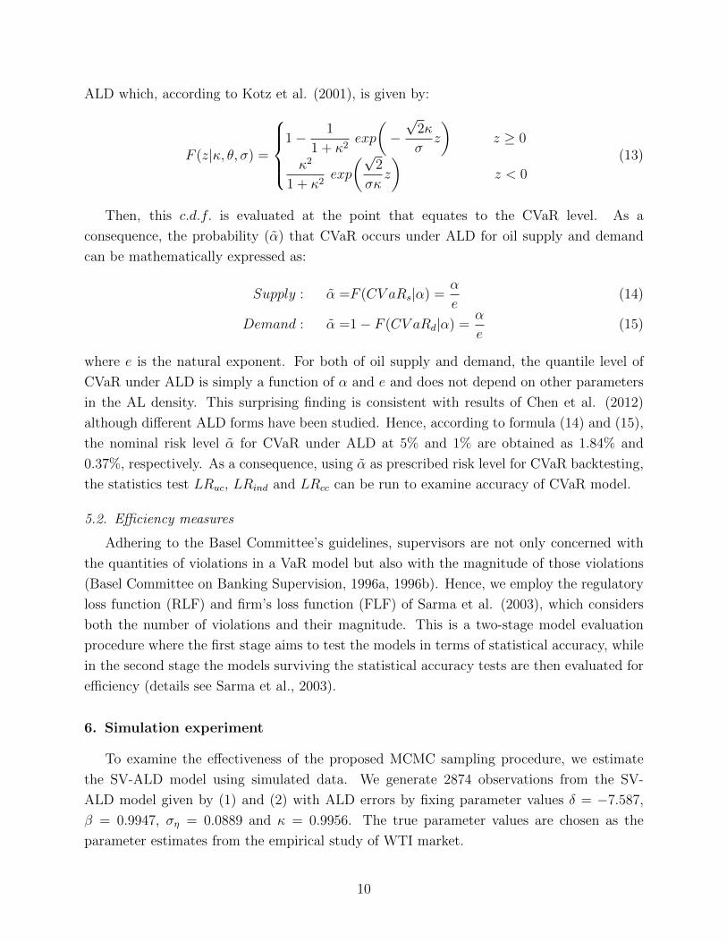
ALD which, according to Kotz et al. (2001), is given by:

F (z|κ, θ, σ) =

1− 1

1 + κ2exp

(−√

2κ

σz

)z ≥ 0

κ2

1 + κ2exp

(√2

σκz

)z < 0

(13)

Then, this c.d.f. is evaluated at the point that equates to the CVaR level. As a

consequence, the probability (α) that CVaR occurs under ALD for oil supply and demand

can be mathematically expressed as:

Supply : α =F (CV aRs|α) =α

e(14)

Demand : α =1− F (CV aRd|α) =α

e(15)

where e is the natural exponent. For both of oil supply and demand, the quantile level of

CVaR under ALD is simply a function of α and e and does not depend on other parameters

in the AL density. This surprising finding is consistent with results of Chen et al. (2012)

although different ALD forms have been studied. Hence, according to formula (14) and (15),

the nominal risk level α for CVaR under ALD at 5% and 1% are obtained as 1.84% and

0.37%, respectively. As a consequence, using α as prescribed risk level for CVaR backtesting,

the statistics test LRuc, LRind and LRcc can be run to examine accuracy of CVaR model.

5.2. Efficiency measures

Adhering to the Basel Committee’s guidelines, supervisors are not only concerned with

the quantities of violations in a VaR model but also with the magnitude of those violations

(Basel Committee on Banking Supervision, 1996a, 1996b). Hence, we employ the regulatory

loss function (RLF) and firm’s loss function (FLF) of Sarma et al. (2003), which considers

both the number of violations and their magnitude. This is a two-stage model evaluation

procedure where the first stage aims to test the models in terms of statistical accuracy, while

in the second stage the models surviving the statistical accuracy tests are then evaluated for

efficiency (details see Sarma et al., 2003).

6. Simulation experiment

To examine the effectiveness of the proposed MCMC sampling procedure, we estimate

the SV-ALD model using simulated data. We generate 2874 observations from the SV-

ALD model given by (1) and (2) with ALD errors by fixing parameter values δ = −7.587,

β = 0.9947, ση = 0.0889 and κ = 0.9956. The true parameter values are chosen as the

parameter estimates from the empirical study of WTI market.

10

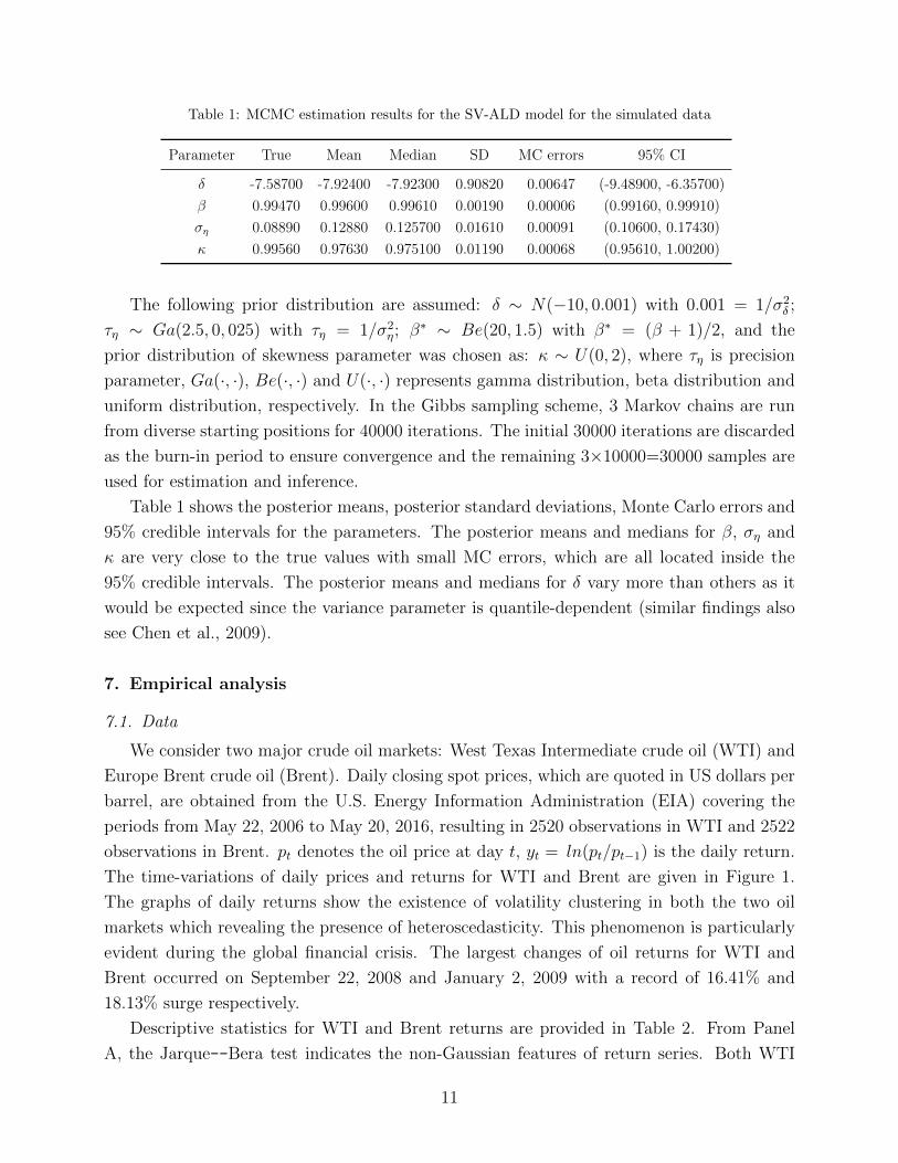
Table 1: MCMC estimation results for the SV-ALD model for the simulated data

Parameter True Mean Median SD MC errors 95% CI

δ -7.58700 -7.92400 -7.92300 0.90820 0.00647 (-9.48900, -6.35700)

β 0.99470 0.99600 0.99610 0.00190 0.00006 (0.99160, 0.99910)

ση 0.08890 0.12880 0.125700 0.01610 0.00091 (0.10600, 0.17430)

κ 0.99560 0.97630 0.975100 0.01190 0.00068 (0.95610, 1.00200)

The following prior distribution are assumed: δ ∼ N(−10, 0.001) with 0.001 = 1/σ2δ ;

τη ∼ Ga(2.5, 0, 025) with τη = 1/σ2η; β

∗ ∼ Be(20, 1.5) with β∗ = (β + 1)/2, and the

prior distribution of skewness parameter was chosen as: κ ∼ U(0, 2), where τη is precision

parameter, Ga(·, ·), Be(·, ·) and U(·, ·) represents gamma distribution, beta distribution and

uniform distribution, respectively. In the Gibbs sampling scheme, 3 Markov chains are run

from diverse starting positions for 40000 iterations. The initial 30000 iterations are discarded

as the burn-in period to ensure convergence and the remaining 3×10000=30000 samples are

used for estimation and inference.

Table 1 shows the posterior means, posterior standard deviations, Monte Carlo errors and

95% credible intervals for the parameters. The posterior means and medians for β, ση and

κ are very close to the true values with small MC errors, which are all located inside the

95% credible intervals. The posterior means and medians for δ vary more than others as it

would be expected since the variance parameter is quantile-dependent (similar findings also

see Chen et al., 2009).

7. Empirical analysis

7.1. Data

We consider two major crude oil markets: West Texas Intermediate crude oil (WTI) and

Europe Brent crude oil (Brent). Daily closing spot prices, which are quoted in US dollars per

barrel, are obtained from the U.S. Energy Information Administration (EIA) covering the

periods from May 22, 2006 to May 20, 2016, resulting in 2520 observations in WTI and 2522

observations in Brent. pt denotes the oil price at day t, yt = ln(pt/pt−1) is the daily return.

The time-variations of daily prices and returns for WTI and Brent are given in Figure 1.

The graphs of daily returns show the existence of volatility clustering in both the two oil

markets which revealing the presence of heteroscedasticity. This phenomenon is particularly

evident during the global financial crisis. The largest changes of oil returns for WTI and

Brent occurred on September 22, 2008 and January 2, 2009 with a record of 16.41% and

18.13% surge respectively.

Descriptive statistics for WTI and Brent returns are provided in Table 2. From Panel

A, the Jarque--Bera test indicates the non-Gaussian features of return series. Both WTI

11

Figure 1: Daily spot prices and returns for WIT and Brent from May 1987 to May 2016

and Brent markets show a mild positive skewness and are leptokurtic or “fat-tailed” with a

significant kurtosis greater than 3. Results from the Ljung--Box Q statistics of order up to

20 indicate the existence of autocorrelation in the datasets. The daily returns series exhibit

significant ARCH effects at 10 and 20 lags at 1% significance level. This aspect will be taken

into account when examining the estimation results. These results can also be immediately

observed from the pattern of return series in Figure 1 where large price movements are

followed by large movements.

Moreover, three tests are employed to examine the stationarity of the time series

before fitting them. Augmented Dicky--Fuller (ADF) test and Phillips--Perron (PP)

test significantly reject the null hypothesis of unit root, and the statistics from the

Kwiatkowski--Phillips--Schmidt--Shin (KPSS) test show that we cannot reject the assumption

of stationarity of the series.

7.2. SV models estimation and comparisons

Convergence diagnostic. Before estimating the parameters from the joint posterior

distribution, convergence diagnostics of the constructed Markov chains in the MCMC

algorithm are conducted using the Brooks--Gelman--Rubin (BGR) diagnostic approach. To

12

Table 2: Descriptive statistics for WTI and Brent oil price returns

WTI Brent

Panel A: Descriptive statistics

Mean -0.000144 -0.000127

Std.dev. 0.024863 0.021998

Maximum 0.164137 0.181297

Minimum -0.128267 -0.168320

Skewness 0.1567 0.1443

Kurtosis 7.6122 8.8043

J-B test 2243.0570*** 3547.5790***

Q(10) 30.6030*** 16.9600*

Q(20) 60.8980*** 54.2270***

ARCH(10) 475.9680*** 215.7230***

ARCH(20) 575.8620*** 409.0370***

Panel B: Unit roots and stationarity tests

ADF -51.4930*** -48.9570***

PP -51.5220*** -48.9660***

KPSS 0.0507 0.0690

Note: Q(l) are Ljung--Box statistics for up to lth order serial correlation.Test statistics of ARCH are obtained using chi-squared distribution. ADFand PP are statistics of the Augmented Dickey--Fuller and Phillips--Perronunit root tests. The largest value from the first 8 lags of KPSS test is listed. ∗,∗∗ and ∗∗∗ denote rejection of null hypothesis at 10%, 5% and 1% significantlevel respectively.

complete a Bayesian paradigm, the prior distribution of the estimated SV model parameters

are set as: δ ∼ N(−10, 0.001) with 0.001 = 1/σ2δ ; τη ∼ Ga(2.5, 0, 025) with τη = 1/σ2

η;

β∗ ∼ Be(20, 1.5) with β∗ = (β + 1)/2, and the prior distribution of skewness parameter

are chosen as: κ ∼ U(0, 2), where τη is precision parameter, Ga(·, ·), Be(·, ·) and U(·, ·)represents gamma distribution, beta distribution and uniform distribution, respectively.9

After discarding the corresponding burn-in period in each SV-type models, the remaining

simulated samples are used to construct posterior inferences.

9The sensitivity analysis indicates that the changing of prior numbers have minor influence on the posteriordistributions of the parameters (δ, β and ση). The setting priors here are those which can facilitate ourposterior inference and enable the speed of convergence to become faster.

13

Table 3: Posterior summary statistics for the parameters in SV-t, SV-N and SV-ALD models

Market Parameter Mean SD MC error 95% CI

SV-t

WTI

ν 13.42000 2.83100 0.13450 (9.24600,20.10000)

δ -9.77200 0.34470 0.00298 (-10.44000,-9.08500)

β 0.99830 0.00101 0.00002 (0.99580,0.99970)

ση 0.09595 0.01143 0.00060 (0.07470,0.11840)

Brent

ν 12.61000 2.50600 0.11710 (8.78900,18.43000)

δ -9.76700 0.34190 0.00300 (-10.43000,-9.09200)

β 0.99850 0.00094 0.00002 (0.99620,0.99980)

ση 0.08333 0.01086 0.00058 (0.06549,0.10730)

SV-N

WTI

µ 0.00037 0.00034 0.00000 (-0.00030,0.00103)

δ -9.76100 0.34660 0.00298 (-10.43000,-9.06800)

β 0.99780 0.00122 0.00003 (0.99490,0.99950)

ση 0.11760 0.01360 0.00072 (0.09209,0.14630)

Brent

µ 0.00013 0.00031 0.00000 (-0.00046,0.00074)

δ -9.78700 0.34210 0.00277 (-10.45000,-9.10000)

β 0.99860 0.00089 0.00002 (0.99640,0.99980)

ση 0.08933 0.01019 0.00054 (0.07112,0.11030)

SV-ALD

WTI

κ 0.99560 0.01592 0.00083 (0.96590,1.02800)

δ -7.58700 0.48730 0.00408 (-8.42200,-6.69800)

β 0.99470 0.00224 0.00005 (0.98990,0.99870)

ση 0.08891 0.00992 0.00051 (0.07065,0.10810)

Brent

κ 0.99820 0.01206 0.00061 (0.97510,1.02200)

δ -7.75000 0.56200 0.00587 (-8.66000,-6.69600)

β 0.99590 0.00184 0.00004 (0.99200,0.99910)

ση 0.07351 0.00812 0.00042 (0.06106,0.09410)

14

Table 4: Posterior summary statistics for the parameters in SV-t-L, SV-N-L and SV-ALD-L models

Market Parameter Mean SD MC error 95% CI

SV-t-L

WTI

ρ -0.62110 0.07616 0.00422 (-0.75940, -0.47680)

ν 10.90000 1.63300 0.06735 (8.22400, 14.50000)

δ -9.71700 0.35290 0.00376 (-10.39000, -9.01300)

β 0.99830 0.00091 0.00002 (0.99610, 0.99960)

ση 0.09112 0.01027 0.00058 (0.07171, 0.10950)

Brent

ρ -0.57170 0.07303 0.00396 (-0.69400, -0.42250)

ν 12.38000 2.79900 0.13860 (8.56100, 19.59000)

δ -9.75300 0.34420 0.00327 (-10.42000, -9.07100)

β 0.9986 0.00084 0.00002 (0.99650, 0.99970)

ση 0.08100 0.00946 0.00053 (0.06535, 0.10170)

SV-N-L

WTI

ρ -0.54850 0.07225 0.00387 (-0.66870,-0.39170)

µ -0.00009 0.00035 0.00001 (-0.00078,0.00059)

δ -9.73200 0.35170 0.00310 (-10.41000,-9.02700)

β 0.99810 0.00100 0.00002 (0.99570,0.99960)

ση 0.11110 0.01034 0.00057 (0.09117,0.13000)

Brent

ρ -0.62630 0.05649 0.00300 (-0.74130,-0.51490)

µ -0.00025 0.00031 0.00000 (-0.00085,0.00035)

δ -9.78400 0.34170 0.00304 (-10.45000,-9.10800)

β 0.99880 0.00070 0.00001 (0.99710,0.99980)

ση 0.08544 0.00821 0.00045 (0.07289,0.10570)

SV-ALD-L

WTI

ρ -0.74780 0.05345 0.00303 (-0.83640,-0.63140)

κ 1.00100 0.01336 0.00077 (0.97690,1.02700)

δ -7.75400 0.38370 0.00485 (-8.46500,-7.12300)

β 0.99550 0.00156 0.00004 (0.99230,0.99840)

ση 0.09288 0.00826 0.00047 (0.07945,0.10980)

Brent

ρ -0.67460 0.06573 0.00369 (-0.78440,-0.53440)

κ 1.00700 0.01282 0.00073 (0.98060,1.02900)

δ -7.91800 0.53680 0.00447 (-8.93000,-6.97100)

β 0.99690 0.00151 0.00005 (0.99340,0.99930)

ση 0.07427 0.00942 0.00055 (0.06148,0.09575)

15

Table 5: WTI: In sample Root Mean Square Error (RMSE)

Year RMSE SV-t RMSE SV-t-L RMSE SV-N RMSE SV-N-L RMSE SV-ALD RMSE SV-ALD-L

2006 0.024666 0.024832 0.024440 0.024392 0.026936 0.026238

2007 0.026485 0.026972 0.026365 0.026705 0.028254 0.029127

2008 0.054977 0.055920 0.054435 0.055954 0.058000 0.056521

2009 0.048405 0.048945 0.048270 0.048405 0.050172 0.049486

2010 0.026399 0.025732 0.026114 0.025974 0.027611 0.027094

2011 0.030133 0.030007 0.030416 0.030359 0.031569 0.031547

2012 0.022471 0.022367 0.022619 0.022762 0.023780 0.024324

2013 0.016566 0.016461 0.016389 0.016542 0.017860 0.017806

2014 0.023295 0.022629 0.023508 0.023643 0.024341 0.024142

2015 0.041619 0.042051 0.041430 0.041656 0.044052 0.044278

2016 0.054839 0.054196 0.054817 0.055393 0.057046 0.057881

Table 6: WTI: In sample Mean Absolute Error (MAE)

Year MAE SV-t MAE SV-t-L MAE SV-N MAE SV-N-L MAE SV-ALD MAE SV-ALD-L

2006 0.019466 0.019450 0.019307 0.019271 0.020534 0.020089

2007 0.020686 0.021100 0.020693 0.021011 0.021565 0.022337

2008 0.038980 0.039382 0.038741 0.039792 0.040603 0.039382

2009 0.035243 0.035479 0.035168 0.035312 0.035673 0.035263

2010 0.020427 0.019900 0.020269 0.020146 0.020922 0.020547

2011 0.023174 0.023026 0.023541 0.023491 0.023819 0.023741

2012 0.017130 0.017094 0.017255 0.017409 0.017748 0.018131

2013 0.013029 0.012923 0.012926 0.013086 0.013686 0.013678

2014 0.016440 0.015911 0.016646 0.016715 0.016746 0.016608

2015 0.032297 0.032592 0.032250 0.032387 0.033461 0.033497

2016 0.042475 0.041849 0.042657 0.042804 0.043476 0.043773

Table 7: Brent: In sample Root Mean Square Error (RMSE)

Year RMSE SV-t RMSE SV-t-L RMSE SV-N RMSE SV-N-L RMSE SV-ALD RMSE SV-ALD-L

2006 0.028946 0.028129 0.028704 0.028340 0.030493 0.028612

2007 0.025080 0.025013 0.024659 0.024954 0.026579 0.028343

2008 0.043941 0.044021 0.044793 0.045493 0.045327 0.051346

2009 0.044852 0.045047 0.044703 0.045426 0.046725 0.048226

2010 0.025725 0.026107 0.025390 0.025443 0.026979 0.026727

2011 0.024890 0.025037 0.024733 0.024698 0.025505 0.028801

2012 0.020495 0.020322 0.020519 0.020438 0.021459 0.023273

2013 0.015774 0.015605 0.015715 0.015712 0.016467 0.017586

2014 0.016807 0.017026 0.016870 0.017287 0.017466 0.020727

2015 0.036134 0.035715 0.035869 0.036038 0.036561 0.041760

2016 0.048917 0.048831 0.048579 0.048513 0.048577 0.054604

16

Table 8: Brent: In sample Mean Absolute Error (MAE)

Year MAE SV-t MAE SV-t-L MAE SV-N MAE SV-N-L MAE SV-ALD MAE SV-ALD-L

2006 0.022680 0.022025 0.022675 0.022358 0.023294 0.021928

2007 0.019715 0.019656 0.019550 0.019745 0.020408 0.021612

2008 0.031998 0.031628 0.032659 0.032980 0.032348 0.035790

2009 0.033279 0.033293 0.033103 0.033729 0.034127 0.034435

2010 0.019849 0.020170 0.019725 0.019820 0.020345 0.020362

2011 0.019328 0.019429 0.019319 0.019302 0.019335 0.021650

2012 0.015935 0.015718 0.016062 0.015953 0.016367 0.017591

2013 0.012273 0.012124 0.012324 0.012326 0.012578 0.013379

2014 0.012167 0.012278 0.012205 0.012469 0.012485 0.014310

2015 0.028058 0.027767 0.028071 0.028192 0.027736 0.031315

2016 0.038214 0.038177 0.038241 0.038077 0.037361 0.041129

Posterior estimates and model comparisons. To compare the fitting ability of

SV-ALD and SV-ALD-L model with conventional SV-N, SV-N-L, SV-t and SV-t-L models,

results of posterior estimates of these models are shown in Table 3 and 4.10 The posterior

means of β in WTI and Brent markets under these models are very close to one, which is

consistent with our general beliefs that there exist a strong persistence of volatility in oil

returns. Our results show that the estimated posterior mean of ση for the SV-ALD model is

lower comparing to the corresponding ση in the SV-N and SV-t model in both of the two oil

markets, and ση in the SV-t model is lower than that ση in the SV-N model.

The estimate for the ση parameter from the SV-ALD-L and SV-t-L model is lower than

the estimate coming from the SV-N-L model. These results are consistent with the findings

from Chib et al. (2002) and Abanto-Valle et al. (2010), indicating that the introduction of

heavy tailed error distribution in the mean equation appears to explain excess returns, thus

decreasing the variance of the volatility process. More importantly, we find statistically

significant negative correlation (ρ < 0) between shocks affecting oil returns and shocks

affecting volatility in the SV-t-L, SV-N-L and the SV-ALD-L specifications. Although

WinBugs can generate deviance information criterion (DIC) values straightforwardly, as

pointed out by Chan and Grant (2016), conditional DIC typically favors over-fitted models

in a series of Monte Carlo experiments. Therefore this cannot be used as a reliable criterion

to compare across models. For this reason, we use various comparison criteria. First of all we

check the in sample RMSE and MAE calculated by year in Table 5 to Table 8.11 Considering

the in sample RMSE and MAE, the SV-N and SV-N-L models outperform the others. Because

this result is not conclusive, in the next sections, we also consider additional criteria such as

10We used the WinBUGS’s code from the website of Yasuhiro Omori as the starting point.11yt is replicated by using the Bayesian estimates for the model parameters and for the volatility.

17

Table 9: Out-of-sample performance for various models: RMSE and MAE for May-December 2016

Market SV-t SV-t-L SV-N SV-N-L SV-ALD SV-ALD-L

RMSE

WTI 0.034910 0.034952 0.033276 0.033010 0.038417 0.035692

Brent 0.038329 0.037781 0.038010 0.037333 0.037907 0.038116

MAE

WTI 0.026940 0.026973 0.025831 0.025362 0.028911 0.026794

Brent 0.029482 0.029095 0.029476 0.028731 0.028495 0.028391

the out-of-sample RMSE and MAE (to test the predictive power of the models) and, more

importantly, the capability of the models to replicate risk in a VaR and CVaR sense.

Out-of-sample performance. Table 9 shows the out-of-sample performance for various

models using the Root Mean square errors (RMSE) and Mean Absolute errors (MAE) criteria.

We used the MCMC estimates from May 2006 to May 2016 to forecast oil returns from the

end of May 2016 to the end of December 2016: the SV-N-L model performs better than

its competitors for both markets if we consider the RMSE criterion (calculated using 500

simulations and fixing the parameters at the MCMC estimates). Considering the MAE

criterion, SV-ALD-L and SV-N-L perform the best.

Table 10 to Table 15 present the results of Engle’s LM ARCH test on the standard

errors for SV-t, SV-t-L, SV-N, SV-N-L, SV-ALD and SV-ALD-L models in both markets.

Considering the series of standard errors, there is no evidence of ARCH effects for the SV-N

model while the SV-N-L model shows ARCH effects in the WTI market at a 1% significance

level. This result gives an opportunity to increase efficiency by modeling ARCH, but does

not violate any assumptions made when estimating the underlying model. As a conclusion,

the SV-N model is the most efficient among the set of models that have been studied in

this paper. From Table 16 to Table 21, we can see that the Kolmogorov Smirnov test for

normality does not reject its null for the Brent standard errors resulting from the SV-t, SV-

t-L, SV-N and SV-N-L models at the 1% significance level. For the WTI standard errors,

it does not reject its null hypothesis of normality for the SV-N and SV-N-L standard errors

at 1% significance level. The Shapiro Francia test (1972) for normality concurs with those

judgements for the standard errors coming from all the models. The Box Pierce portmanteau

(or Q) test for white noise rejects its null for both series of standard errors.

Diebold Mariano test. This test calculates a measure of predictive accuracy proposed

by Diebold and Mariano (1995). We ran the test for each of 500 simulations per model

18

Table 10: WTI: Engle’s Lagrange multiplier test for autoregressive conditional heteroskedasticity forstandardised residuals and squared standardised residuals for SV-t and SV-t-L models

1 lag p-val 5 lags p-val 10 lags p-val 30 lags p-val

SV-t res 2.04 0.15 8.98 0.11 13.75 0.18 47.15 0.02

SV-t res squ 0.19 0.66 0.82 0.98 1.66 1.00 11.50 1.00

SV-t-L res 3.51 0.06 9.46 0.09 12.79 0.24 39.48 0.12

SV-t-L res squ 0.09 0.76 0.57 0.99 0.98 1.00 31.60 0.39

Table 11: WTI: Engle’s Lagrange multiplier test for autoregressive conditional heteroskedasticity forstandardised residuals and squared standardised residuals for SV-N and SV-N-L models

1 lag p-val 5 lags p-val 10 lags p-val 30 lags p-val

SV-N res 0.00 0.95 16.21 0.01 27.56 0.00 77.20 0.00

SV-N res squ 0.03 0.87 1.99 0.85 4.29 0.93 19.90 0.92

SV-N-L res 0.24 0.63 11.73 0.04 20.67 0.02 60.18 0.00

SV-N-L res squ 0.07 0.79 1.23 0.94 3.07 0.98 18.77 0.94

Table 12: WTI: Engle’s Lagrange multiplier test for autoregressive conditional heteroskedasticity forstandardised residuals and squared standardised residuals for SV-ALD and SV-ALD-L models

1 lag p-val 5 lags p-val 10 lags p-val 30 lags p-val

SV-ALD res 7.31 0.01 9.72 0.08 11.20 0.34 35.24 0.23

SV-ALD res squ 0.63 0.43 1.04 0.96 1.49 1.00 13.45 1.00

SV-ALD-L res 13.69 0.00 15.75 0.01 18.05 0.05 39.41 0.12

SV-ALD-L res squ 7.55 0.01 8.13 0.15 8.62 0.57 36.25 0.20

Table 13: Brent: Engle’s Lagrange multiplier test for autoregressive conditional heteroskedasticity forstandardised residuals and squared standardised residuals for SV-t and SV-t-L models

1 lag p-val 5 lags p-val 10 lags p-val 30 lags p-val

SV-t res 5.40 0.02 17.55 0.00 26.16 0.00 50.28 0.01

SV-t res squ 0.69 0.41 3.92 0.56 5.91 0.82 33.66 0.29

SV-t-L res 5.35 0.02 14.18 0.01 21.18 0.02 43.89 0.05

SV-t-L res squ 0.51 0.47 3.36 0.64 5.18 0.88 27.70 0.59

19

Table 14: Brent: Engle’s Lagrange multiplier test for autoregressive conditional heteroskedasticity forstandardised residuals and squared standardised residuals for SV-N and SV-N-L models

1 lag p-val 5 lags p-val 10 lags p-val 30 lags p-val

SV-N res 7.17 0.01 22.48 0.00 34.65 0.00 70.86 0.00

SV-N res squ 1.22 0.27 6.91 0.23 10.47 0.40 31.61 0.39

SV-N-L res 5.38 0.02 13.79 0.02 21.96 0.02 47.77 0.02

SV-N-L res squ 0.78 0.38 4.29 0.51 7.01 0.72 22.95 0.82

Table 15: Brent: Engle’s Lagrange multiplier test for autoregressive conditional heteroskedasticity forstandardised residuals and squared standardised residuals for SV-ALD and SV-ALD-L models

1 lag p-val 5 lags p-val 10 lags p-val 30 lags p-val

SV-ALD res 0.94 0.33 6.24 0.28 9.97 0.44 26.97 0.62

SV-ALD res squ 0.10 0.75 1.42 0.92 2.64 0.99 35.76 0.22

SV-ALD-L res 2.70 0.10 8.02 0.15 11.89 0.29 28.67 0.54

SV-ALD-L res squ 0.33 0.56 1.81 0.87 2.84 0.98 14.38 0.99

Table 16: WTI: Test Statistics and P-values for standardised residuals and squared standardised residualsfor SV-t and SV-t-L models

KSmirnov p-val SFrancia p-val Qtest p-val

SV-t res 0.011 0.940 3.514 0.000 33.011 0.775

SV-t res squ 0.263 0.000 15.592 0.000 44.168 0.300

SV-t-L res 0.019 0.346 5.281 0.000 33.544 0.755

SV-t-L res squ 0.276 0.000 15.857 0.000 43.892 0.310

Table 17: WTI: Test Statistics and P-values for standardised residuals and squared standardised residualsfor SV-N and SV-N-L models

KSmirnov p-val SFrancia p-val Qtest p-val

SV-N res 0.009 0.988 0.414 0.340 33.470 0.758

SV-N res squ 0.245 0.000 15.165 0.000 54.062 0.068

SV-N-L res 0.016 0.576 2.627 0.004 33.652 0.750

SV-N-L res squ 0.253 0.000 15.339 0.000 47.908 0.183

20

Table 18: WTI: Test Statistics and P-values for standardised residuals and squared standardised residualsfor SV-ALD and SV-ALD-L models

KSmirnov p-val SFrancia p-val Qtest p-val

SV-ALD res 0.015 0.587 4.652 0.000 32.453 0.796

SV-ALD res squ 0.273 0.000 15.766 0.000 40.367 0.454

SV-ALD-L res 0.020 0.241 5.749 0.000 34.901 0.699

SV-ALD-L res squ 0.280 0.000 15.907 0.000 45.253 0.262

Table 19: Brent: Test Statistics and P-values for standardised residuals and squared standardised residualsfor SV-t and SV-t-L models

KSmirnov p-val SFrancia p-val Qtest p-val

SV-t res 0.022 0.177 2.716 0.003 43.504 0.325

SV-t res squ 0.257 0.000 15.268 0.000 48.892 0.158

SV-t-L res 0.024 0.115 2.820 0.002 43.906 0.310

SV-t-L res squ 0.257 0.000 15.277 0.000 46.316 0.228

Table 20: Brent: Test Statistics and P-values for standardised residuals and squared standardised residualsfor SV-N and SV-N-L models

KSmirnov p-val SFrancia p-val Qtest p-val

SV-N res 0.021 0.201 1.865 0.031 43.025 0.343

SV-N res squ 0.250 0.000 15.102 0.000 56.556 0.043

SV-N-L res 0.023 0.156 2.340 0.010 42.681 0.357

SV-N-L res squ 0.253 0.000 15.175 0.000 47.479 0.194

Table 21: Brent: Test Statistics and P-values for standardised residuals and squared standardised residualsfor SV-ALD and SV-ALD-L models

KSmirnov p-val SFrancia p-val Qtest p-val

SV-ALD res 0.024 0.122 4.169 0.000 43.549 0.323

SV-ALD res squ 0.266 0.000 15.449 0.000 35.039 0.693

SV-ALD-L res 0.025 0.084 3.799 0.000 43.420 0.328

SV-ALD-L res squ 0.264 0.000 15.439 0.000 35.317 0.681

21

Table 22: Diebold Mariano test: comparison of forecast accuracy over 500 out-of-sample predictions

Variable Observations Mean SD Min Max

WTI

SV-t vs SV-t-L

r1t 41 0.0010954 0.0004075 0.0006428 0.0023901

r2t 41 0.0011213 0.0003617 0.0005928 0.0022897

SV-N vs SV-N-L

r1t 241 0.0012336 0.0005985 0.0005911 0.0046736

r2t 241 0.0012112 0.0008895 0.0005486 0.0103819

SV-ALD vs SV-ALD-L

r1t 240 0.001657 0.0006006 0.0007806 0.0045232

r2t 240 0.0012848 0.0008002 0.0006352 0.0051321

Brent

SV-t vs SV-t-L

r1t 46 0.0014817 0.0004475 0.0008498 0.0028845

r2t 46 0.001352 0.000371 0.000789 0.0025136

SV-N vs SV-N-L

r1t 258 0.0015684 0.0006906 0.0007161 0.0063691

r2t 258 0.0014911 0.0008635 0.0006984 0.0078067

SV-ALD vs SV-ALD-L

r1t 209 0.0015392 0.0006215 0.0007717 0.0041496

r2t 209 0.00158 0.000905 0.0007069 0.0090912

and present summary statistics from that set of test results. Given an actual series and

two competing predictions, one may apply a loss criterion (such as squared error or absolute

error) and then calculate a number of measures of predictive accuracy that allow the null

hypothesis of equal accuracy to be tested. Table 22 reports the results where the r1 and

r2 variables are the MSEs for model 1 (non-leverage model) and model 2 (leverage model),

respectively. If the p− value < 0.05, the test rejects the null that the two models are equally

capable in terms of their MSEs. For the simulations in which the test rejects equal forecast

accuracy, we can compare the mean MSE for the two models.

For the WTI data, in the case of SV-t vs SV-t-L models, we can observe 41 rejections

(over 500 out-of-sample simulations): model 1 (the non-leverage model) has the smaller

mean MSE. Considering SV-N vs SV-N-L models, we can observe 241 rejections: model 2

(the leverage model) has the smaller mean MSE. Considering SV-ALD vs SV-N-ALD models,

we can observe 240 rejections: model 2 (the leverage model) has the smaller mean MSE. For

the Brent data, in the case of SV-t vs SV-t-L models, we can observe 46 rejections: model

2 (the leverage model) has the smaller mean MSE. Considering SV-N vs SV-N-L models,

22

we can observe 258 rejections: model 2 (the leverage model) has the smaller mean MSE.

Considering SV-ALD vs SV-N-ALD models, we can observe 209 rejections: model 1 (the

non-leverage model) has the smaller mean MSE.

In summary, in four of the six simulations, model 2 (the leverage model) has the smaller

mean MSE for those simulations in which the Diebold–Mariano test rejects its null hypothesis

of equal forecast accuracy.

7.3. Selection of VaR and CVaR models

We now focus on the models for which we have the most evidence of a substantial impact

of the introduction of leverage on the prediction accuracy of the model (SV-N, SV-N-L,

SV-ALD and SV-ALD-L models). In order to classify the competing models, we follow a

two-stage model evaluation procedure where in the first stage models are selected in terms of

their statistical accuracy (backtesting stage), while in the second stage the surviving models

are evaluated in terms of their efficiency (efficiency stage).12

Stage 1: Backtesting VaR and CVaR model. The Failure Rate (FR) or violation

rate, computes the ratio of the number of times oil returns exceed the estimated VaRs over

the total number of observations. The model is said to be correctly specified if the calculated

ratio is equal to the pre-specified VaR level α (i.e. 5% and 1%). If the Failure Rate is

greater than α, we can conclude that the model underestimates the risk, and vice versa (see

Marimoutou et al., 2009; Aloui and Mabrouk, 2010; Louzis et al., 2014).

A criterion for evaluating our results comes from the consideration that a conservative

investor (see for example, Zhao et al., 2015 and Hung et al., 2008) might choose a greater

confidence level and estimate a relatively greater risk (corresponding to α = 5% in the

VaR definition), while a more speculative investor might estimate a smaller risk and face a

relatively smaller confidence level (corresponding to α = 1% in the VaR definition).

In order to backtest the accuracy of the estimated VaRs, three formal tests are conducted

based on the criteria of the empirical failure rates. Table 23 shows the VaR backtesting

summary results of SV-N, SV-ALD, SV-N-L and SV-ALD-L models for the WTI and Brent

market, considering both supply and demand risks. According to the LRind test, the null

hypothesis that exceptions are independent cannot be rejected at the two risk levels in the

two markets for both the four models by considering oil supply and demand risk, suggesting

that there are not many/no consecutive violations. Modelling the data using SV-N and SV-

N-L models, the test LRuc and LRcc are passed, which indicates the capability of the models

of estimating tail risks. The SV-ALD and SV-ALD-L models overestimate the tail risk and

the null hypothesis of tests LRuc and LRcc are rejected in WTI market and partly rejected in

12For details see Sarma et al. (2003).

23

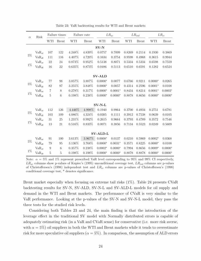
Table 23: VaR backtesting results for WTI and Brent markets

α RiskFailure times Failure rate LRuc LRind LRcc

WTI Brent WTI Brent WTI Brent WTI Brent WTI Brent

SV-N

5%VaRst 107 122 4.248% 4.839% 0.0757 0.7099 0.8269 0.2114 0.1930 0.3869

VaRdt 111 116 4.407% 4.720% 0.1634 0.3754 0.9598 0.4968 0.3615 0.9944

1%VaRst 22 24 0.873% 0.952% 0.5138 0.8071 0.5334 0.5334 0.6598 0.7559

VaRdt 16 22 0.635% 0.873% 0.0486 0.5113 0.6510 0.6591 0.1282 0.6524

SV-ALD

5%VaRst 77 98 3.057% 3.887% 0.0000∗ 0.0077 0.6766 0.9211 0.0000∗ 0.0265

VaRdt 82 97 3.255% 3.848% 0.0000∗ 0.0057 0.4314 0.2596 0.0001∗ 0.0108

1%VaRst 7 8 0.278% 0.317% 0.0000∗ 0.0001∗ 0.8434 0.8214 0.0001∗ 0.0003∗

VaRdt 5 6 0.198% 0.238% 0.0000∗ 0.0000∗ 0.8878 0.8656 0.0000∗ 0.0000∗

SV-N-L

5%VaRst 112 126 4.446% 4.998% 0.1940 0.9964 0.3700 0.4934 0.2751 0.6781

VaRdt 103 109 4.086% 4.324% 0.0305 0.1111 0.3912 0.7538 0.0639 0.0105

1%VaRst 31 25 1.231% 0.992% 0.2615 0.9664 0.3793 0.4789 0.3572 0.7546

VaRdt 13 21 0.516% 0.833% 0.0071 0.3856 0.7134 0.5523 0.0249 0.5609

SV-ALD-L

5%VaRst 91 100 3.613% 3.967% 0.0008∗ 0.0137 0.0210 0.5969 0.0002∗ 0.0368

VaRdt 79 95 3.136% 3.768% 0.0000∗ 0.0031∗ 0.3571 0.8225 0.0000∗ 0.0108

1%VaRst 9 6 0.357% 0.238% 0.0002∗ 0.0000∗ 0.7994 0.8656 0.0009∗ 0.0000∗

VaRdt 5 5 0.198% 0.198% 0.0000∗ 0.0000∗ 0.8878 0.8878 0.0000∗ 0.0000∗

Note: α = 5% and 1% represent prescribed VaR level corresponding to 95% and 99% CI respectively,LRuc columns show p-values of Kupiec’s (1995) unconditional coverage test, LRind columns are p-valuesof Christoffersen’s (1998) independent test and LRcc columns are p-values of Christoffersen’s (1998)conditional coverage test, * denotes significance.

Brent market especially when focusing on extreme tail risks (1%). Table 24 presents CVaR

backtesting results for SV-N, SV-ALD, SV-N-L and SV-ALD-L models for oil supply and

demand in the WTI and Brent markets. The performance of CVaR is very similar to the

VaR performance. Looking at the p-values of the SV-N and SV-N-L model, they pass the

three tests for the studied risk levels.

Considering both Tables 23 and 24, the main finding is that the introduction of the

leverage effect in the traditional SV model with Normally distributed errors is capable of

adequately estimating risk (in a VaR and CVaR sense) for conservative (i.e. more risk averse,

with α = 5%) oil suppliers in both the WTI and Brent markets while it tends to overestimate

risk for more speculative oil suppliers (α = 5%). In comparison, the assumption of ALD errors

24

Table 24: CVaR backtesting results for WTI and Brent markets

α RiskFailure times Failure rate LRuc LRind LRcc

WTI Brent WTI Brent WTI Brent WTI Brent WTI Brent

SV-N

1.96%CVaRst 41 43 1.628% 1.706% 0.2152 0.3463 0.2440 0.2216 0.2315 0.2887

CVaRdt 33 45 1.310% 1.785% 0.0123∗ 0.5199 0.3492 0.2006 0.0278 0.3396

0.38%CVaRst 10 10 0.397% 0.397% 0.8906 0.8926 0.7776 0.7776 0.9481 0.9409

CVaRdt 7 9 0.278% 0.357% 0.3816 0.8496 0.8434 0.7994 0.6669 0.9408

SV-ALD

1.84%CVaRst 19 15 0.754% 0.595% 0.0000∗ 0.0000∗ 0.5909 0.6716 0.0000∗ 0.0000∗

CVaRdt 11 19 0.437% 0.754% 0.0000∗ 0.0000∗ 0.7560 0.5909 0.0000∗ 0.0000∗

0.37%CVaRst 2 2 0.079% 0.079% 0.0035∗ 0.0035∗ 0.9550 0.9550 0.0142 0.0141

CVaRdt 3 0 0.119% 0.000% 0.0155 0.0000∗ 0.9326 1.0000 0.0533 0.0001∗

SV-N-L

1.96%CVaRst 45 54 1.786% 2.142% 0.5235 0.5159 0.2006 0.8780 0.3533 0.7499

CVaRdt 32 40 1.270% 1.587% 0.0077∗ 0.1621 0.3641 0.2558 0.0187∗ 0.1881

0.38%CVaRst 12 14 0.476% 0.555% 0.4495 0.1809 0.7346 0.6924 0.7060 0.3715

CVaRdt 6 9 0.238% 0.357% 0.2140 0.8496 0.8656 0.7994 0.4544 0.9408

SV-ALD-L

1.84%CVaRst 24 15 0.953% 0.595% 0.0003∗ 0.0000∗ 0.4967 0.6716 0.0010∗ 0.0000∗

CVaRdt 8 17 0.318% 0.674% 0.0000∗ 0.0000∗ 0.8213 0.6307 0.0000∗ 0.0000∗

0.37%CVaRst 3 2 0.119% 0.079% 0.0155 0.0035∗ 0.9326 0.9550 0.0533 0.0141

CVaRdt 3 1 0.119% 0.040% 0.0155 0.0005∗ 0.9326 0.9775 0.0533 0.0022∗

Note: α = 1.96% and 0.38% corresponds to 5% and 1% risk level of Normal distribution and α = 1.84%and 0.37% corresponds to 5% and 1% risk level of ALD. LRuc columns show p-values of Kupiec’s (1995)unconditional coverage test, LRind columns are p-values of Christoffersen’s (1998) independent test and LRcc

columns are p-values of Christoffersen’s (1998) conditional coverage test, * denotes significance.

leads to overestimating risk for both type of investors.

Stage 2: Efficiency Measures. Lopez (1998, 1999) was the first to propose the

comparison between VaR models on the basis of their ability to minimise some specific loss

function which reflected a specific objective of the risk manager.

Adhering to the Basel Committee’s guidelines, supervisors are not only concerned with

the number of violations in a VaR model but also with the magnitude of those violations

(Basel Committee on Banking Supervision, 1996a, 1996b). In order to address this aspect,

following Sarma et al. (2003), we compare the relevant models in terms of the Regulatory Loss

Function (RLF) which focuses on the magnitude of the failure and in terms of the Firm’s

Loss Function (FLF) which, while giving relevance to the magnitude of failures, imposes an

25

Table 25: RLF and FLF Loss function approach applied to the models surviving the VaR backtesting stage

Volatility modelsand VaR methods

RLF FLF

5% 1% 5% 1%

WTI Brent WTI Brent WTI Brent WTI Brent

Panel A: Average loss values

SV-NSupply 0.000209 0.000199 0.000170 0.000182 0.001709 0.001555 0.000328 0.002279

Demand 0.000251 0.000237 0.000501 0.000227 -0.001680 -0.001531 -0.000499 -0.002274

SV-N-LSupply 0.000239 0.000203 0.000176 0.000192 0.001755 0.001586 0.000353 0.002317

Demand 0.000229 0.000219 0.000511 0.000162 -0.001733 -0.001569 -0.000511 -0.002313

SV-ALDSupply - 0.000250 - - - 0.001681 - -

Demand - - - - - - - -

SV-ALD-LSupply - 0.000235 - - - 0.001716 - -

Demand - - - - - - - -

Panel B: Sign statistics

SABSupply 47.2408 46.9433 49.1934 49.4129 -13.0107∗ -11.6517∗ -9.9422∗ -9.2612∗

Demand 48.8746 49.0146 49.9904 49.9307 12.0144 10.6155 9.5438 8.8230

SBASupply 48.4363 48.1382 49.9505 49.8909 13.0107 11.6517 9.9422 9.2612

Demand 46.8822 46.5051 49.7115 49.5722 -12.0144∗ -10.6155∗ -9.5438∗ -8.8230∗

SCDSupply - 48.1382 - - - -7.1102∗ - -

Demand - - - - - - - -

SDCSupply - 47.8594 - - - 7.1102 - -

Demand - - - - - - - -

Note: This table compares the best performing models in the VaR backtesting procedure following the Regulatoryloss function (RLF) and Firm’s loss function (FLF). Panel A presents the average loss values for RLF and FLFfor the competing models at different risk levels in the two oil markets. The models with the lowest average lossvalues are underlined. Panel B reports the standardized sign statistics values. SAB denotes the standardized signstatistics with null of “non-superiority” of SV-N over SV-N-L, SBA represents the standardized sign statistics withnull of “non-superiority” of SV-N-L over SV-N, SCD is the standardized sign statistics with null hypothesis of “non-superiority” of SV-ALD over SV-ALD-L while SDC is the standardized sign statistics with null hypothesis of “non-superiority” of SV-ALD-L over SV-ALD. * means significance in the corresponding level.

additional penalty related to the opportunity cost of capital.13 We use a non-parametric sign

test to check the ability the relevant VaR models to minimize these loss functions.14

Table 25 presents the summary results for the RLF and FLF loss function approach as

applied to the models chosen in the VaR backtesting stage. The results in Panel A show that

the SV-N model achieves the smallest value of average loss more often than the SV-N-L model

while the outcome is not conclusive for the SV-ALD model and the SV-ALD-L model under

the two approaches. To examine the statistical significance of the losses, we report the values

of the standardized sign test in Panel B. Considering the RLF criterion, this test shows that

the competing models (leverage vs no-leverage models) are not significantly different from

13This criterion penalizes large failures more than small failures (See Sarma et al., 2003).14For the sign test see Lehmann (1974), Diebold and Mariano (1995), Hollander and Wolfe (1999) and

Sarma et al. (2003).

26

Table 26: RLF and FLF Loss function approach applied to the models surviving the CVaR backtestingstage

Volatility modelsand CVaR methods

RLF FLF

1.84%/1.96% 0.37%/0.38% 1.84%/1.96% 0.37%/0.38%

WTI Brent WTI Brent WTI Brent WTI Brent

Panel A: Average loss values

SV-NSupply 0.000167 0.000201 0.000143 0.000136 0.000877 0.000796 0.000222 0.000204

Demand - - 0.000284 0.000167 - - -0.001221 -0.000203

SV-N-LSupply 0.000228 0.000189 0.000226 0.000129 0.000881 0.000794 0.000224 0.000204

Demand - - 0.000301 0.000100 - - -0.000222 -0.000203

SV-ALDSupply - - - - - - - -

Demand - - 0.000094 - - - -0.000317 -

SV-ALD-LSupply - - - - - - - -

Demand - - 0.000107 - - - -0.000310 -

Panel B: Sign statistics

SABSupply 48.5160 48.4171 49.7115 49.7714 1.3748 2.5294 0.6974 1.6531

Demand - - 50.1099 50.0502 - - -1.0958 -1.7726

SBASupply 49.8708 49.7714 50.1896 50.0502 -1.3748 -2.5294∗ -0.6974 -1.6531

Demand - - 49.9904 49.9706 - - 1.0958 1.7726

SCDSupply - - - - - - - -

Demand - - 50.1498 - - - -10.8190∗ -

SDCSupply - - - - - - - -

Demand - - 50.0701 - - - 10.8190

Note: This table compares the best performing models in the CVaR backtesting procedure following the Regulatoryloss function (RLF) and Firm’s loss function (FLF). Panel A presents the average loss values of RLF and FLFfor the competing models at different risk levels in the two oil markets. The models with the lowest average lossvalues are underlined. Panel B reports the standardized sign statistics values. SAB denotes the standardized signstatistics with null of “non-superiority” of SV-N over SV-N-L, SBA represents the standardized sign statistics withnull of “non-superiority” of SV-N-L over SV-N, SCD is the standardized sign statistics with null hypothesis of“non-superiority” of SV-ALD over SV-ALD-L while SDC is the standardized sign statistics with null hypothesisof “non-superiority” of SV-ALD-L over SV-ALD. The nominal risk level 1.84% and 0.37% corresponds to 5%and 1% risk level of ALD and 1.96% and 0.38% corresponds to 5% and 1% of the Normal distribution. * meanssignificance in the corresponding nominal level.

each others which means that the choice of financial regulators, both on the supply and on

the demand side, would not be affected by the introduction of leverage. Considering Panel B

for the FLF criterion, for both the WTI and Brent markets, the SV-N model is significantly

better than the SV-N-L model for firms involved with oil supply while the SV-N-L model

is significantly better than the SV-N model for firms interested in oil demand. This means

that the introduction of leverage (SV-N-L) would be useful for firms who are on the demand

side for oil in both the WTI and Brent markets, who use VaR for risk management and who

are particularly worried about the magnitude of the losses exceeding VaR while wanting to

minimize the opportunity cost of capital. Using the same logic, firms who are on the supply

side, would be better off not considering the leverage effect.

27

Table 26 shows the summary results of RLF and FLF loss function approach applied to

the models chosen in the CVaR backtesting stage. In terms of the average economic losses

and considering both RLF and FLF as selection criteria, the SV-N model performs relatively

better than the SV-N-L model in the WTI market while in the Brent market, the SV-N-L

model outperforms the SV-N model. The standardized sign test values by FLF in the Panel

B indicate that in most cases there are no significant differences between the competitors.

The only exception is that the SV-N-L model outperforms the SV-N model for oil supply in

the Brent market at 1.96% risk level and the SV-ALD model performs better for oil demand

in the WTI market at 0.37%

8. Conclusions

In this paper, we study the interaction between oil returns and volatility by using daily

spot returns in the crude oil markets (both WTI and Brent) with a particular consideration

for the impact of the leverage effect on measures of risk such as VaR and CVaR. We find

that, allowing for leverage, traditional SV models with Normal distributed errors provide the

best predictions in our out of sample experiments.

In order to address the risk faced by oil suppliers and oil consumers we model spot crude

oil returns using Stochastic Volatility (SV) models with various error distributions. Among

other cases, we test the assumption of Asymmetric Laplace Distributed (ALD) errors in order

to model in a more distinctive way the type of risk faced by oil suppliers versus the risk faced

by oil buyers.

We find that the introduction of the leverage effect in the traditional SV model with

Normally distributed errors is capable of adequately estimating risk (in a VaR and CVaR

sense) for conservative (i.e. more risk averse, with α = 5%) oil suppliers in both the WTI

and Brent markets while it tends to overestimate risk for more speculative oil suppliers

(α = 1%). In comparison, the assumption of ALD errors leads to overestimating risk for both

type of investors. In the model efficiency selection stage, our results show that the choice

of financial regulators, both on the supply and on the demand side, would not be affected

by the introduction of leverage. Focusing instead on firm’s internal risk management, our

results show that the introduction of leverage (SV-N-L model) would be useful for firms who

are on the demand side for oil (in both the WTI and Brent markets), who use VaR for risk

management and who are particularly worried about the magnitude of the losses exceeding

VaR while wanting to minimize the opportunity cost of capital. Using the same logic, firms

who are on the supply side, would be better off not considering the leverage effect (SV-N

model).

28

References

Abanto-Valle, C. A., Bandyopadhyay, D., Lachos, V.H. and Enriquez, I. (2010). Robust

Bayesian analysis of heavy-tailed stochastic volatility models using scale mixtures of normal

distributions. Computational Statistics & Data Analysis, 54(12), 2883-2898.

Aloui, C. and Mabrouk, S. (2010). Value-at-Risk estimations of energy commodities via

long-memory, asymmetry and fat-tailed GARCH models. Energy Policy, 38(5), 2326-2339.

Artzner, P., Delbaen, F., Eber, J. and Heath, D. (1999). Coherent measures of risk.

Mathematical Finance, 9(3), 203-228.

Basel Committee on Banking Supervision. 1996a. Amendment to the Capital Accord to

incorporate market risks. Bank for International Settlements, Basel.

Basel Committee on Banking Supervision. 1996b. Supervisory framework for the use

of backtesting in conjunction with the internal models approach to market risk capital

requirements. Publication No. 22, Bank for International Settlements, Basel.

Breidt, F. J., Crato, N. and De Lima, P. (1998). The detection and estimation of long

memory in stochastic volatility. Journal of Econometrics, 83(1), 325-348.

Cappuccio, N., Lubian, D. and Raggi, D. (2004). MCMC Bayesian estimation of a skew-

GED stochastic volatility model. Studies in Nonlinear Dynamics & Econometrics, 8(2).

Chai, J., Guo, Ju-e., Gong L. and Wang S. Y. (2011). Estimating crude oil price ’Value at

Risk’ using the Bayesian-SV-SGT approach. Systems Engineering-Theory & Practice, 31(1).

Chan, J. C. (2013). Moving average stochastic volatility models with application to inflation

forecast. Journal of Econometrics, 176(2), 162-172.

Chan, J. C. (2017). The stochastic volatility in mean model with time-varying parameters:

An application to inflation modeling. Journal of Business & Economic Statistics, 35(1),

17-28.

Chan, J. C. and Grant, A. L. (2016a). Modeling energy price dynamics: GARCH versus

stochastic volatility. Energy Economics, 54, 182-189.

Chan, J. C. and Grant, A. L. (2016b). On the observed-data deviance information criterion

for volatility modeling. Journal of Financial Econometrics, 14(4), 772-802.

Chan, J. C. and Grant, A. L. (2016c). Fast computation of the deviance information criterion

for latent variable models. Computational Statistics & Data Analysis, 100, 847-859.

29

Chan, J. C. and Hsiao, C. Y.-L. (2013). Estimation of Stochastic Solatility

Models with Heavy Tails and Serial Dependence. [Online]. Available at

https://papers.ssrn.com/sol3/papers.cfm?abstract id=2359838 [Accessed 27 October

2017].

Chen, C. W., Gerlach, R. and Wei, D. (2009). Bayesian causal effects in quantiles:

Accounting for heteroscedasticity. Computational Statistics & Data Analysis, 53(6), 1993-

2007.

Chen, Q., Gerlach, R. and Lu, Z. (2012). Bayesian Value-at-Risk and expected shortfall

forecasting via the asymmetric Laplace distribution. Computational Statistics & Data

Analysis, 56(11), 3498-3516.

Chib, S., Nardari, F. and Shephard, N. (2002). Markov chain Monte Carlo methods for

stochastic volatility models. Journal of Econometrics, 108(2), 281-316.

Christoffersen, P. F. (1998). Evaluating interval forecasts. International Economic Review,

841-862.

Diebold, F. X. and Mariano, R. S. (1995). Comparing predictive accuracy. Journal of

Business and Economic Statistics, 13, 253-263.

Fan, Y., Zhang, Y. -J., Tsai, H. -T. and Wei, Y. -M. (2008). Estimating Value at Riskof

crude oil price and its spillover effect using the GED-GARCH approach. Energy Economics,

30(6), 3156-3171.

Hollander, M. and Wolfe, D. A. (1999). Nonparametric Statistical Methods. 2nd edn. New

York: John Wiley.

Hung, J.-C., Lee, M.-C. and Liu, H.-C. (2008). Estimation of value-at-risk for energy

commodities via fat-tailed GARCH models. Energy Economics, 30(3), 1173-1191.

Koopman, S. J. and Hol Uspensky, E. (2002). The stochastic volatility in mean model:

empirical evidence from international stock markets. Journal of Applied Econometrics,

17(6), 667-689.

Kotz, S., Kozubowski, T. and Podgorski, K. (2001). The Laplace distribution and

generalizations: a revisit with applications to communications, economics, engineering, and

finance. New York: Springer Science & Business Media.

Kristoufek, L. (2014). Leverage effect in energy futures. Energy Economics, 45, 1-9.

Kupiec, P. H. (1995). Techniques for verifying the accuracy of risk measurement models.

The Journal of Derivatives, 3(2), 73-84.

30

Lardic, S. and Mignon, V. (2008). Oil prices and economic activity: An asymmetric

cointegration approach. Energy Economics, 30(3), 847-855.

Lehmann, E. L. (1974). Nonparametrics. New York: Holden-Day Inc. McGraw-Hill.

Lopez, J. A. (1998). Testing your risk tests. Financial Survey, 18-20.

Lopez, J. A. (1999). Methods for evaluating Value-at-Risk estimates. Federal Reserve Bank

of San Francisco Economic Review, 2, 3-17.

Louzis, D. P., Xanthopoulos-Sisinis, S. and Refenes, A. P. (2014). Realized volatility models

and alternative Value-at-Risk prediction strategies. Economic Modelling, 40, 101-116.

Marimoutou, V., Raggad, B. and Trabelsi, A. (2009). Extreme value theory and value at

risk: application to oil market. Energy Economics, 31(4), 519-530.

Papapetrou, E. (2001). Oil price shocks, stock market, economic activity and employment

in Greece. Energy Economics, 23(5), 511-532.

Sarma, M., Thomas, S. and Shah, A. (2003). Selection of Value-at-Risk models. Journal of

Forecasting, 22, 337-358.

So, M. E. P., Lam, K. and Li, W. K. (1998). A stochastic volatility model with Markov

switching. Journal of Business & Economic Statistics, 16(2), 244-253.

Takahashi, M., Omori, Y. and Watanabe, T. (2009). Estimating stochastic volatility models

using daily returns and realized volatility simultaneously. Computational Statistics & Data

Analysis, 53(6), 2404-2426.

Wichitaksorn, N., Wang, J. J., Boris Choy, S. T. and Gerlach, R. (2015). Analyzing return

asymmetry and quantiles through stochastic volatility models using asymmetric Laplace

error via uniform scale mixtures. Applied Stochastic Models in Business and Industry, 31(5),

584-608.

Youssef, M., Belkacem, L. and Mokni, K. (2015). Value-at-Risk estimation of energy

commodities: A long-memory GARCHEVT approach. Energy Economics, 51, 99-110.

Yu, J. and Yang, Z. (2002). A class of nonlinear stochastic volatility models. Univ. of

Auckland, Economics Working Paper, (229).

Zhao, S., Lu, Q., Han, L., Liu, Y. and Hu, F. (2015). A mean-CVaR-skewness portfolio

optimization model based on asymmetric Laplace distribution. Annals of Operations

Research, 226(1), 727-739.

31

A. Asymmetric Laplace distribution

A random variable X is said to follow an Asymmetric Laplace Distribution if the

characteristic function of X can be defined as:

ψ (t) =1

1 + 12σ2t2 − iµt

(16)

where i is the imaginary unit, t ∈ R is the argument of the characteristic function, σ is the

scale parameter with σ > 0 and µ is the mean of X. Then, we have X ∼ AL(µ, σ). Note

that this characteristic function is a standardized form with location parameter θ = 0. An

equivalent notation for the distribution of X can be written as AL(µ, τ). More details can

refer to Kotz et al. (2001).

The density function is given by:

f(z|κ, σ, θ) =

√

2

τ

κ

1 + κ2exp(−

√2κ

τ(z − θ)) z ≥ θ

√2

τ

κ

1 + κ2exp(

√2

τκ(z − θ)) z < θ

(17)

B. VaR and CVaR derivation for oil supply and demand under SV-ALD

For oil supply, we have:

P (yt ≤ −V aRs,t|Ωt) = P

(yt − µσt

≤ −V aRs,t − µσt

∣∣∣∣Ωt

)= P

(zt ≤ −ms,q = −V aRs,t + µ

σt

)=

∫ −ms,q−∞

f−(zt) dzt

=

∫ −ms,q−∞

√2

τ

κ

1 + κ2exp(

√2ztτκ

) dzt

=

√2

τ

κ

1 + κ2

∫ −ms,q−∞

τκ√2d(exp(

√2ztτκ

))

=κ2

1 + κ2

(exp(

√2(−ms,q)

τκ)− exp(

√2(−∞)

κτ)

)=

κ2

1 + κ2exp(

√2(−ms,q)

κτ) = α

where f−(zt) is the negative part of the p.d.f. of ALD. Transforming this equation and setting

τ = 1, we can obtain the VaR for oil supply:

V aRs,t = −µ+ms,qσt = −µ− κσt√2lnα(1 + κ2)

κ2(18)

32

and further the CVaR for oil supply:

CV aRs,t =− E [yt|yt ≤ −V aRs,t] = V aRs,t +κσt√

2(19)

For oil demand, we have:

P (yt > V aRd,t|Ωt) = P

(yt − µσt

>V aRd,t − µ

σt

∣∣∣∣Ωt

)= P

(zt > md,q =

V aRd,t − µσt

)=

∫ +∞

md,q

f+(zt) dzt

=

∫ +∞

md,q

√2

τ

κ

1 + κ2exp(−

√2κztτ

) dzt

=

√2

τ

κ

1 + κ2

∫ +∞

md,q

−τ√2κd(exp(−

√2κztτ

))

= − 1

1 + κ2

(exp(−

√2κ(+∞)

τ)− exp(−

√2κmd,q

τ)

)=

1

1 + κ2exp(−

√2κmd,q

τ) = α

where f+(zt) is the positive part of the p.d.f. of ALD. Transforming this equation and setting

τ = 1, we can obtain the VaR for oil demand:

V aRd,t = µ+md,qσt = µ− σt√2κ

ln(α(1 + κ2)) (20)

and further the CVaR for oil demand:

CV aRd,t = E [yt|yt > V aRd,t] = V aRd,t +σt√2κ

(21)

C. Derivation of the pdf of scaled ALD

Consider a random variable z follows the Asymmetric Laplace density function in equation

(17) with mean and variance given by:15

E(z) = θ +τ√2

(1

κ− κ) V ar(z) =

τ 2

2(

1

κ2+ κ2)

15More details of the mean and variance can refer to Kotz et al. (2001) for more details.

33

where τ = σ in our setting and is a constant, then we can transform z into another random

variable εt by taking:

εt =z√

V ar(z)(22)

Taking partial derivatives of εt with respect to z, then we have:

dz =√V ar(z) dεt =

τ√2

√1 + κ4

κdεt (23)

In the case z ≥ 0 or εt ≥ 0, by substituting (22) and (23) into density function (17), we are

able to obtain:

Pr+(εt) =

∫ +∞

0

√2

τ

κ

1 + κ2

τ√2

√1 + κ4

κexp(−√

2κ

τ

τ√2

√1 + κ4

κ(εt − θ)) dεt

=

∫ +∞

0

√1 + κ4

1 + κ2exp(−

√1 + κ4 (εt − θ)) dεt

(24)

Similarly, in the case z < 0 or εt < 0, it has:

Pr−(εt) =

∫ 0

−∞

√2

τ

κ

1 + κ2

τ√2

√1 + κ4

κexp(

√2

τκ

τ√2

√1 + κ4

κ(εt − θ)) dεt

=

∫ 0

−∞

√1 + κ4

1 + κ2exp(

√1 + κ4

κ2(εt − θ)) dεt

(25)

As a result, the pdf of SALD of random variable εt given σt can be written as:16

f(εt|κ, θ, σt) =

√

1 + κ4

1 + κ2

1

σtexp(−√

1 + κ4

σt(εt − θ)) εt ≥ θ

√1 + κ4

1 + κ2

1

σtexp(

√1 + κ4

κ2σt(εt − θ)) εt < θ

(26)

where κ is skewness parameter and σt is the time-varying volatility of return series.

16Note that parameter τ has been canceled out in this derivation.

34

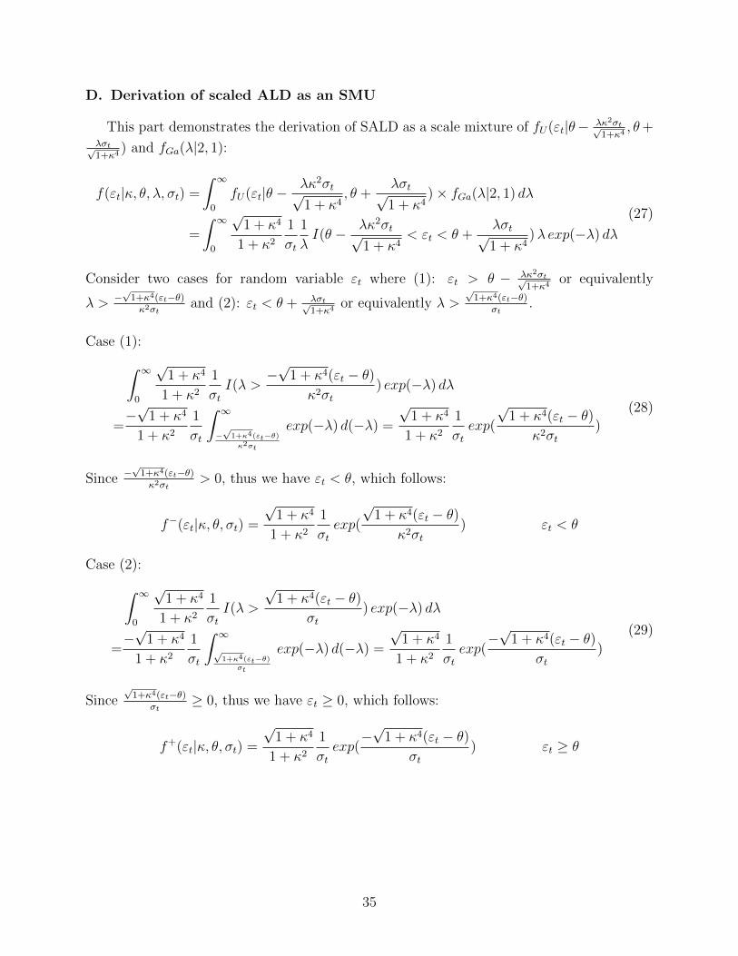
D. Derivation of scaled ALD as an SMU

This part demonstrates the derivation of SALD as a scale mixture of fU(εt|θ− λκ2σt√1+κ4

, θ+λσt√1+κ4

) and fGa(λ|2, 1):

f(εt|κ, θ, λ, σt) =

∫ ∞0

fU(εt|θ −λκ2σt√1 + κ4

, θ +λσt√1 + κ4

)× fGa(λ|2, 1) dλ

=

∫ ∞0

√1 + κ4

1 + κ2

1

σt

1

λI(θ − λκ2σt√

1 + κ4< εt < θ +

λσt√1 + κ4

)λ exp(−λ) dλ

(27)

Consider two cases for random variable εt where (1): εt > θ − λκ2σt√1+κ4

or equivalently

λ > −√

1+κ4(εt−θ)κ2σt

and (2): εt < θ + λσt√1+κ4

or equivalently λ >√

1+κ4(εt−θ)σt

.

Case (1):∫ ∞0

√1 + κ4

1 + κ2

1

σtI(λ >

−√

1 + κ4(εt − θ)κ2σt

) exp(−λ) dλ

=−√

1 + κ4

1 + κ2

1

σt

∫ ∞−√

1+κ4(εt−θ)κ2σt

exp(−λ) d(−λ) =

√1 + κ4

1 + κ2

1

σtexp(

√1 + κ4(εt − θ)

κ2σt)

(28)

Since −√

1+κ4(εt−θ)κ2σt

> 0, thus we have εt < θ, which follows:

f−(εt|κ, θ, σt) =

√1 + κ4

1 + κ2

1

σtexp(

√1 + κ4(εt − θ)

κ2σt) εt < θ

Case (2):∫ ∞0

√1 + κ4

1 + κ2

1

σtI(λ >

√1 + κ4(εt − θ)

σt) exp(−λ) dλ

=−√

1 + κ4

1 + κ2

1

σt

∫ ∞√

1+κ4(εt−θ)σt

exp(−λ) d(−λ) =

√1 + κ4

1 + κ2

1

σtexp(−√

1 + κ4(εt − θ)σt

)

(29)

Since√

1+κ4(εt−θ)σt

≥ 0, thus we have εt ≥ 0, which follows:

f+(εt|κ, θ, σt) =

√1 + κ4

1 + κ2

1

σtexp(−√

1 + κ4(εt − θ)σt

) εt ≥ θ

35

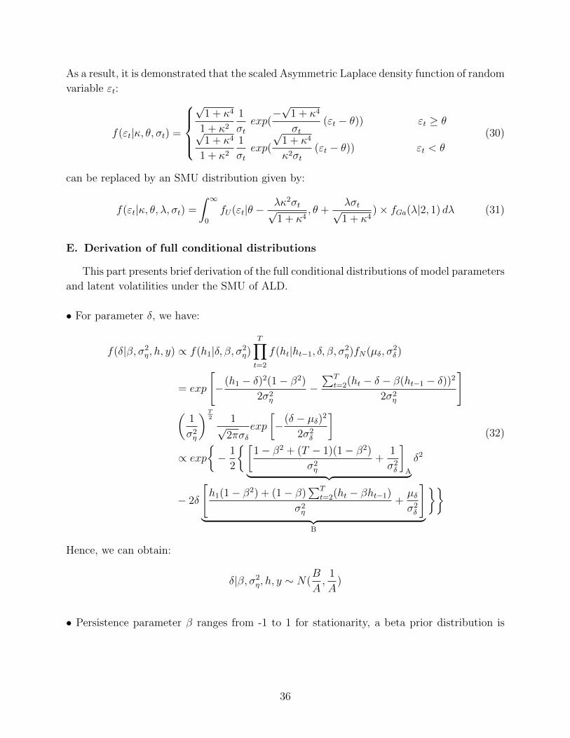
As a result, it is demonstrated that the scaled Asymmetric Laplace density function of random

variable εt:

f(εt|κ, θ, σt) =

√

1 + κ4

1 + κ2

1

σtexp(−√

1 + κ4

σt(εt − θ)) εt ≥ θ

√1 + κ4

1 + κ2

1

σtexp(

√1 + κ4

κ2σt(εt − θ)) εt < θ

(30)

can be replaced by an SMU distribution given by:

f(εt|κ, θ, λ, σt) =

∫ ∞0

fU(εt|θ −λκ2σt√1 + κ4

, θ +λσt√1 + κ4

)× fGa(λ|2, 1) dλ (31)

E. Derivation of full conditional distributions

This part presents brief derivation of the full conditional distributions of model parameters

and latent volatilities under the SMU of ALD.

• For parameter δ, we have:

f(δ|β, σ2η, h, y) ∝ f(h1|δ, β, σ2

η)T∏t=2

f(ht|ht−1, δ, β, σ2η)fN(µδ, σ

2δ )

= exp

[−(h1 − δ)2(1− β2)

2σ2η

−∑T

t=2(ht − δ − β(ht−1 − δ))2

2σ2η

](

1

σ2η

)T2 1√

2πσδexp

[−(δ − µδ)2

2σ2δ

]∝ exp

− 1

2

[1− β2 + (T − 1)(1− β2)

σ2η

+1

σ2δ

]A︸ ︷︷ ︸ δ

2

− 2δ

[h1(1− β2) + (1− β)

∑Tt=2(ht − βht−1)

σ2η

+µδσ2δ

]︸ ︷︷ ︸

B

(32)

Hence, we can obtain:

δ|β, σ2η, h, y ∼ N(

B

A,

1

A)

• Persistence parameter β ranges from -1 to 1 for stationarity, a beta prior distribution is

36

assigned to β∗ = β+12∼ Be(aβ, bβ), then we have:

f(β∗|δ, σ2η, h, y) ∝ f(h1|δ, β, σ2

η)T∏t=2

f(ht|ht−1, δ, β, σ2η)fBe(aβ, bβ)

= exp

[−(h1 − δ)2(1− β2)

2σ2η

−∑T

t=2(ht − δ − β(ht−1 − δ))2

2σ2η

](

1

σ2η

)T2 β∗(aβ−1)(1− β∗)(bβ−1)

B(aβ, bβ)

∝ exp

[β∑T

t=2(ht − 1)(ht−δ − δ)σ2η

+β2[(h1 − δ)2 −

∑Tt=2(ht−1 − δ)2]

2σ2η

](1 + β)(aβ−1)(1− β)(bβ−1)

(33)

where B(·, ·) is beta function with B(aβ, bβ) =Γ(aβ)Γ(bβ)

Γ(aβ+bβ), and Γ(·) is gamma function.

• For parameter σ2η, we have:

f(σ2η|δ, β, h, y) ∝ f(h1|δ, β, σ2

η)T∏t=2

f(ht|ht−1, δ, β, σ2η)fIG(aσ, bσ)

=1√

2σ2η

1−β2πexp

−(h1 − δ)2

2σ2η

1−β2

1√2σ2

ηπ

exp

[−∑T

t=2(ht − δ − β(ht−1 − δ))2

2σ2η

]baσσ

Γ(aσ)σ2(−aσ−1)η exp

(− bσσ2η

)

∝ exp

[−bσ + 1

2(h1 − δ)2(1− β2) + 1

2

∑Tt=2(ht − δ − β(ht−1 − δ))2

σ2η

](

1

σ2η

)(aσ+T2

)+1

(34)

Therefore, we can obtain:

σ2η|δ, β, h, y ∼ IG(aσ, bσ)

where aσ = aσ + T2

and bσ = bσ + 12(h1 − δ)2(1− β2) + 1

2

∑Tt=2(ht − δ − β(ht−1 − δ))2.

37

• For latent variables ht, we have:

f(ht|h−t, δ, β, σ2η, y) ∝ f(y|ht, δ, β, σ2

η)f(ht|h−t, δ, β, σ2η)

=1

λeht/2√1+κ4

+ λκ2eht/2√1+κ4

1√2πB2

exp

[−(ht − A)2

2B2

]∝ e−

ht2 exp

[−1

2

(h2t

B2− 2ht

A

B2

)]

= exp

− 1

2

1

B2︸︷︷︸C

h2t − 2ht

(A

B2− 1

2

)︸ ︷︷ ︸

D

(35)

where

A = δ +β[(ht−1 − δ) + (ht+1 − δ)]

1 + β2, B2 =

σ2η

1 + β2

is the mean and variance of Normal density function fN(ht|A,B2), which has equality:

f(ht|h−t, δ, β, σ2η) = f(ht|ht−1, ht+1, δ, β, σ

2η) = fN(ht|A,B2)

Hence, it can be shown that:

ht|h−t, δ, β, σ2η, y ∼ N(

D

C,B2) or N(A− B2

2, B2) (36)

38