LEVEL SET PERCOLATION FOR RANDOM INTERLACEMENTS

AND THE GAUSSIAN FREE FIELD

Pierre-Francois Rodriguez1

Abstract

We consider continuous-time random interlacements on Zd, d ≥ 3, and investigate the

percolation model where a site x of Zd is occupied if the total amount of time spent at xby all the trajectories of the interlacement at level u ≥ 0 exceeds some constant α ≥ 0,and empty otherwise. We also investigate percolation properties of empty sites. A recentisomorphism theorem [15] enables us to “translate” some of the relevant questions intothe language of level-set percolation for the Gaussian free field on Z

d, d ≥ 3, about whichnew insights of independent interest are also gained.

December 2013

1Departement Mathematik, ETH Zurich, CH-8092 Zurich, Switzerland.

This research was supported in part by the grant ERC-2009-AdG 245728-RWPERCRI.

0 Introduction

In the present work, we consider the field of occupation times for continuous-time randominterlacement at level u ≥ 0 on Z

d, d ≥ 3, and investigate the percolative properties ofthe random subset of Z

d obtained by keeping only those sites at which the occupationtime exceeds some given cut-off value α ≥ 0. We also consider the percolative propertiesof the complement of this set in Z

d. Our main interest is to infer for which values of theparameters (u, α) these random sets percolate. A recent isomorphism theorem [15] relatesthe field of occupation times for continuous-time random interlacements on Z

d, d ≥ 3(and more generally, on any transient weighted graph) to the Gaussian free field on thesame graph. We will exploit this correspondence as a transfer mechanism to reformulatesome of the problems in terms of questions regarding level-set percolation for the Gaussianfree field. This will allow us to use certain renormalization techniques recently developedin this context in [11]. Additionally, we derive new results concerning “two-sided” level-set percolation for the Gaussian free field on Z

d, d ≥ 3, where, in contrast to (0.2) of[11] (see also [2]), the level sets consist of those sites at which the absolute value of thecorresponding field variable exceeds a certain level h ≥ 0.

We now describe our results and refer to Section 1 for details. We consider continuous-time random interlacements on Z

d, d ≥ 3. Somewhat informally, this model can be definedas a cloud of simple random walk trajectories modulo time-shift on Z

d constituting aPoisson point process, where a non-negative parameter u appearing multiplicatively inthe intensity measure regulates how many paths enter the picture (we defer a precisedefinition to the next section, see the discussion around (1.8)). For any u ≥ 0 and α ≥ 0,we introduce the (random) subsets of Zd

(0.1) Iu,α = x ∈ Zd ;Lx,u > α, Vu,α = x ∈ Z

d ;Lx,u ≤ α = Zd \ Iu,α,

where (Lx,u)x∈Zd denotes the field of occupation times at level u, see (1.15), and ask forwhich values of the parameters u and α these sets percolate. Note that for all u ≥ 0, Iu,0

corresponds to the (discrete-time) interlacement set at level u introduced in (0.7) of [14](see also (1.9) and (1.16) below) and Vu,0 to the according vacant set. Before addressingthe core issue of describing the phase diagrams for percolation of the random sets Iu,α andVu,α, as u and α vary, we prove uniqueness of the infinite clusters, whenever they exist.More precisely, we show in Corollary 2.6 that for all u ≥ 0, α > 0 and d ≥ 3,

(0.2) P-a.s., Iu,α and Vu,α contain at most one infinite connected component,

where P denotes the law of the interlacement point process, as defined below (1.8). Forα = 0, (0.2) is already known and follows from [14], Corollary 2.3, and [17], Theorem 1.1.

Our main results concern the existence/absence of infinite clusters inside Iu,α andVu,α, in terms of the parameters u and α. Let us define the functions

(0.3) ηI(u, α) = P[0

Iu,α

←→∞], ηV(u, α) = P

[0

Vu,α

←→∞], for u ≥ 0, α ≥ 0,

to denote the probabilities that 0 lies in an infinite cluster of Iu,α and Vu,α, respectively.Observing that ηI(u, α) is decreasing in α for every (fixed) value of u ≥ 0, it is sensible tointroduce the critical parameter

(0.4) α∗(u) = infα ≥ 0 ; ηI(u, α) = 0 ∈ [0,∞], for u ≥ 0

1

(with the convention inf ∅ = ∞). It is not difficult to see that the function α∗(·) is non-decreasing, see (5.1) below. Our main results regarding percolation of the sets Iu,α statethat

(0.5) 0 < α∗(u) <∞, for all u > 0 and d ≥ 3

(see Theorem 3.1 for positivity of α∗(u) and Theorem 5.1 for finiteness). In words, thesets Iu,α exhibit a non-trivial percolation phase transition as α varies, for every (fixed)positive value of u.

In a similar vein, for Vu,α, we introduce the critical parameter

(0.6) u∗(α) = infu ≥ 0 ; ηV(u, α) = 0 ∈ [0,∞], for α ≥ 0,

which is well-defined since ηV(·, α) is non-increasing for every value of α ≥ 0 (we willcomment on the asymmetry in the role of u and α in (0.4) and (0.6) below; see thediscussion following (0.14)). It is an easy matter to verify that the function u∗(·) isnon-decreasing, see (5.6), and that u∗(0) = u∗, where u∗ refers to the critical point forpercolation of the vacant set of (discrete-time) random interlacements, as defined in (0.13)of [14], which is known to be finite and strictly positive for all dimensions d ≥ 3, see[14], Theorem 4.3, and [13], Theorem 3.4 (see also Theorem 5.1 in [16] for a more generalresult). Our main conclusion concerning percolation of the sets Vu,α, see Theorem 5.2below, asserts that

(0.7) (0 < u∗ ≤) u∗(α) <∞, for all α ≥ 0 and d ≥ 3.

In fact, not only are we able to establish finiteness of the critical parameters in (0.5) and(0.7), but also the stronger result that (see (5.3), (5.8) and Remark 5.4)

the connectivity functions P[0

Iu,α

←→ x]

and P[0

Vu,α

←→ x]

have stretched

exponential decay in x as |x| → ∞, for all u ≥ 0 and α = α(u) sufficiently large,

respectively for all α ≥ 0 and u = u(α) sufficiently large,

(0.8)

where the events in the probabilities refer to the existence of a nearest-neighbor path inIu,α, resp. Vu,α, connecting x to the origin. Tentative phase diagrams for percolation ofIu,α and Vu,α, u, α ≥ 0, can be found in Figure 1 below.

As hinted above, some of the proofs rely on Theorem 0.1 of [15], which relates (Lx,u)x∈Zd

to the Gaussian free field on Zd, see (0.14). In particular, en route to proving (0.8), we

show the following result, interesting in its own right. Let PG denote the canonical law ofGaussian free field on Z

d, i.e. PG is the probability measure on RZd

such that,

under PG, the canonical field ϕ = (ϕx)x∈Zd is a centered Gaussian

field with covariance E[ϕxϕy] = g(x, y), for all x, y ∈ Zd,

(0.9)

where g(·, ·) denotes the Green function of simple random walk on Zd, cf. (1.1). For

arbitrary h ≥ 0, we consider the “two-sided” level set

(0.10) L≥h = x ∈ Zd ; |ϕx| ≥ h.

Introducing the critical parameter

(0.11) h∗ = infh ≥ 0 ; PG[0

L≥h

←→∞] = 0,

2

I(u, α) :

α∗(u)

α∗∗(u)

1

10

0

V (u, α) :

u∗∗(α)

u∗(α)αα

u∗ u∗∗ uu

Figure 1: the functions I(u, α) = 1P-a.s., Iu,α has a unique infinite component and V (u, α) =1P-a.s., Vu,α has a unique infinite component. The shaded areas, in which the correspondingconnectivity functions have stretched exponential decay, define the auxiliary critical lines α∗∗(u)and u∗∗(α), see Remark 5.4, 2). It is presently an open problem whether the two critical linesα∗(·) and α∗∗(·), respectively u∗(·) and u∗∗(·), actually coincide.

we show in Theorem 4.7 that

(0.12) h∗ <∞, for all d ≥ 3,

and, similarly to (0.8), that the connectivity function of L≥h has stretched exponentialdecay for sufficiently large h, see (4.53). This strengthens the result (0.5) of [11] (see also[2]), which states that h∗, the critical level for percolation of the (one-sided) level setsx ∈ Z

d ; ϕx ≥ h, h ∈ R, is finite for all d ≥ 3. Moreover, it follows from Theorem 3.3 of[11] that h∗ is strictly positive in large dimensions, see Remark 4.8, 2) below. It was alreadyknown from Theorem 7 in [7] (see also p. 281 therein) that there is no directed percolationinside L≥h when h is sufficiently large, for all d ≥ 4. Finally, let us mention that our resultsconcerning L≥h might be helpful for investigating certain random conductance models onZ

d, in the spirit of [3], with nearest-neighbor conductances involving the Gaussian freefield; see also [5, 6] for further motivation.

We now comment on the proofs. In order to establish the uniqueness result (0.2),cf. Corollary 2.6 below, we invoke a classical theorem of Burton and Keane (see [4],Theorem 2) after showing in Theorem 2.3 that for all u, α > 0, the translation invariantlaw Qu,α of (1x ∈ Iu,α)x∈Zd under P, see (1.18) and Lemma 1.1, has the so-called finiteenergy property, i.e.

(0.13) 0 < Qu,α(Y0 = 1|σ(Yx, x 6= 0)) < 1, Qu,α-a.s. for all u > 0, α > 0 and d ≥ 3,

where Yx, x ∈ Zd, refer to the canonical coordinates on 0, 1Zd

. This differs markedlyfrom the case α = 0, since the law of random interlacement at any level u ≥ 0 fails to fulfillthe finite-energy condition, see [14], Remark 2.2, 3). The proof of the lower bound in (0.13)involves a delicate local “surgery operation” on paths, which roughly consists of sending a“furtive” trajectory to x which spends enough time there to ensure that Lx,u > α withoutspoiling a given configuration outside of x. The proof of the upper bound essentiallyrequires us to prevent x from being visited too much, which is a considerably simpler task.

The positivity of α∗(u) for u > 0 in (0.5), cf. Theorem 3.1 below, is shown as follows.First, we introduce new occupation variables on Z

d, whereby a site x is “occupied” if andonly if x ∈ Iu,0 and the first-passage holding time at x of the trajectory in the interlacementcloud with smallest label (≤ u) passing through x exceeds α (see (3.2) for a precise

3

definition). In particular, this implies that Lx,u > α whenever x is “occupied,” henceQu,α dominates the (joint) law of these new occupation variables. Loosely speaking, wethen prove that, conditionally on Iu,0, these new variables define an independent Bernoullipercolation on the discrete interlacement set Iu,0 with a suitable success parameter p(α)satisfying limα→0 p(α) = 1. This enables us to use some recent results of [9] to infer thatthe set of occupied vertices has an infinite cluster if p(α) is sufficiently close to 1 (i.e. if αis small enough).

The proofs of the finiteness of α∗(u) and u∗(α) in (0.5) and (0.7), see Theorems 5.1 and5.2, respectively, both rely on the aforementioned isomorphism theorem (see [15], Theorem0.1), which states that

(Lx,u +

1

2ϕ2

x

)x∈Zd , under P⊗ PG, has the

same law as(1

2(ϕx +

√2u)2)

x∈Zd , under PG.(0.14)

We focus on the claim α∗(u) < ∞ first. Thus, we consider Iu,α for fixed u ≥ 0, as αbecomes large. By (0.14), Qu,α (the law of (1Lx,u > α)x∈Zd under P) is dominated bythe law of

(1(ϕx +

√2u)2/2 > α)

x∈Zd under PG. Hence, intuitively, if Lx,u > α, then

|ϕx +√

2u| >√

2α, i.e. |ϕx| has to be large (since α is). This heuristic reasoning suggeststhat the asserted finiteness of α∗(u) is in fact a corollary of (0.12).

The proof of (0.7) is somewhat more involved, but has a similar flavor. Suppose thatx ∈ Vu,α, i.e. Lx,u ≤ α, for some fixed α > 0. From the “equality” Lx,u + 1

2ϕ2x “=” 1

2(ϕx +√2u)2, we deduce that, as u → ∞, either ϕ is very negative (as to counteract the effect

of√

2u), or |ϕx| must be large (since Lx,u stays bounded), and both are rather unlikelyby virtue of (0.12). This indicates that a subcritical phase for Vu,α should emerge when ubecomes sufficiently large, cf. also Fig. 1. Note that the preceding discussion also accountsfor the incongruent roles of u and α in the definitions (0.4) and (0.6), which is due to theway we apply (0.14).

Finally, the result (0.12) concerning “two-sided” level-set percolation for the Gaussianfree field, see Theorem 4.7 below, is shown using some of the tools developed in [11] for theanalysis of (one-sided) level-set percolation (i.e. percolation of the sets x ∈ Z

d ; ϕx ≥ h,h ∈ R; the corresponding critical parameter is denoted by h∗, see (0.4) in [11]). Inparticular, it involves a renormalization scheme akin to the one introduced in Section 2 of[11] (see also [12], [16]), and crucially depends on the decoupling inequality (Proposition2.2 in [11]; see also Proposition 4.1 below) derived therein. However, we cannot simplyfollow the strategy used to prove finiteness of h∗ in [11] in order to establish (0.12), because

the relevant crossing events B(0, L)L≥h

←→ S(0, 2L), with L ≥ 1, h ≥ 0, which refer to theexistence of a (nearest-neighbor) path in L≥h connecting B(0, L), the closed ball of radiusL around the origin in the ℓ∞-norm, to S(0, 2L), the ℓ∞-sphere of radius 2L around 0, areneither increasing nor decreasing “in ϕ,” so Proposition 2.2 of [11] does not apply directly.To overcome this difficulty, we proceed as follows. First, we partition Z

d into disjointboxes of equal side length L0, for some L0 ≥ 1, and call any such box h-bad if |ϕx| > h forat least one site x inside the box (this is quite crude but suffices for our purpose). Next,we consider the quantities

q+n (h) “=” PG[the box B(0, Ln) contains 2n “well-separated” boxes of side

length L0, each of which contains at least one site x with ϕx ≥ h],

for h ≥ 0, where (Ln)n≥0 is a geometrically increasing sequence of length scales, see(4.1). We define q−

n (h) similarly, with the last condition replaced by the requirement that

4

ϕx ≤ −h for some site x in the given box of side length L0. Using the results of [11], weshow that limn→∞ q±

n (h) = 0 for some careful choice of the parameters h and Ln, n ≥ 0.Together with a geometric argument in the spirit of Lemma 6 in [9], see Lemmas 4.4and 4.5 below, this yields that large connected components of h-bad blocks have smallprobability. The claim (0.12) then easily follows, since the existence of an infinite clusterin L≥h implies the existence of an infinite connected component of h-bad boxes.

We conclude this introduction by describing the organization of this article. In Sec-tion 1, we introduce some basic notation, briefly review the definition of continuous-time random interlacements, and collect a few auxiliary properties of the measures Qu,α,u, α ≥ 0 (see above (0.13)). Sections 2 and 3 are devoted to the uniqueness result (0.2)(see Corollary 2.6) and to the positivity of α∗ in (0.5) (see Theorem 3.1), respectively.All results concerning absence of percolation are contained in Sections 4 and 5. Section 4deals solely with the Gaussian free field, and (0.12) is shown in Theorem 4.7, after a suit-able renormalization scheme has been set up. Section 5 addresses the question of absenceof percolation for the sets Iu,α and Vu,α. The main results (0.5) and (0.7) are estab-lished in Theorems 5.1 and 5.2, respectively, along with the asserted decay behavior of thecorresponding connectivity functions, see (0.8).

One final remark concerning our convention regarding constants: we denote by c, c′, . . .positive constants with values changing from place to place. Numbered constants c0, c1, . . .are defined at the place they first occur within the text and remain fixed from then onuntil the end of the article. The dependence of constants (and other quantities) on thedimension d of the lattice will be kept implicit throughout.

1 Notation and useful results

In this section, we introduce some basic notation to be used in the sequel, recall the defi-nition of continuous-time random interlacement on Z

d, d ≥ 3, and collect some auxiliaryproperties of the law Qu,α of Iu,α (see (1.18) below), for u, α ≥ 0.

We denote by N = 0, 1, 2, . . . the set of natural numbers, by N∗ = N \ 0 the setof positive integers and by Z = . . . ,−1, 0, 1, . . . the set of integers. We write R forthe set of real numbers, R+ for the set of non-negative real numbers (this includes 0),abbreviate r ∧ s = minr, s and r ∨ s = maxr, s for any two numbers r, s ∈ R, and [r]for the integer part of r, for any r ≥ 0. We consider the lattice Z

d, and (tacitly) assumethroughout that d ≥ 3. On Z

d, we respectively denote by | · | and | · |∞ the Euclideanand ℓ∞-norms. For any x ∈ Z

d and r ≥ 0, we let B(x, r) = y ∈ Zd ; |y − x|∞ ≤ r

and S(x, r) = y ∈ Zd ; |y − x|∞ = r stand for the ℓ∞-ball and ℓ∞-sphere of radius r

centered at x. Given K and U subsets of Zd, Kc = Zd \K stands for the complement of

K in Zd, |K| for the cardinality of K, K ⊂⊂ Z

d means that K ⊂ Zd and |K| < ∞, and

d(K,U) = inf|x − y|∞ ; x ∈ K, y ∈ U denotes the ℓ∞-distance between K and U . IfK = x, we simply write d(x,U). Finally, for any K ⊂ Z

d, we define the inner boundaryof K to be the set ∂iK = x ∈ K ; ∃y ∈ Kc, |y − x| = 1, and the outer boundary of Kas ∂K = ∂i(Kc).

We endow Zd with the nearest-neighbor graph structure, i.e. the edge-set consists of

all pairs of sites x, y, x, y ∈ Zd, such that |x − y| = 1. We consider the spaces W+, W

of infinite, respectively doubly infinite, Zd × (0,∞)-valued sequences, such that the Zd-

valued sequences form an infinite, respectively doubly-infinite nearest-neighbor trajectoryspending finite time in any finite subset of Zd, and such that the (0,∞)-valued componentshave an infinite sum in the case of W+, and infinite “forward” and “backward” sums,when restricted to positive and negative indices, in the case of W . We write Xn, σn and

5

θn with n ≥ 0, respectively n ∈ Z, for the Zd- and (0,∞)-valued canonical coordinates

and canonical shifts on W+, respectively W , and denote by W+ and W the correspondingcanonical σ-algebras. For w ∈ W , we will often abbreviate X(w) = (Xn(w))n∈Z andσ(w) = (σn(w))n∈Z.

We let Px, x ∈ Zd, be the law on W+ under which (Xn)n≥0 is distributed as simple

random walk starting at x and σn, n ≥ 0, are i.i.d. exponential variables with parameter1, independent of the Xn, n ≥ 0. Since d ≥ 3, the walk is transient, so W+ has fullmeasure under Px. We denote by Ex the corresponding expectation. Moreover, for anymeasure ρ on Z

d, we write Pρ for the measure∑

x∈Zd ρ(x)Px, and Eρ for the correspondingexpectation. We denote by g(·, ·) the Green function of simple random walk, i.e.

(1.1) g(x, y) =∑

n≥0

Px[Xn = y], for x, y ∈ Zd,

which is finite (since d ≥ 3) and symmetric. Moreover, g(x, y) = g(x − y, 0)def.= g(x − y)

due to translation invariance. For U ⊆ Zd and w ∈ W+, we write HU (w), HU (w) and

TU (w) for the entrance time in U , the hitting time of U and the exit time from U for thetrajectory w, i.e.

(1.2) HU (w) = infn ≥ 0 ; Xn(w) ∈ U, HU (w) = infn ≥ 1 ; Xn(w) ∈ U, TU = HUc .

We define HU (w) and TU (w) in a similar fashion when w ∈ W , with “n ∈ Z” replacing“n ≥ 0” in (1.2), and simply write Hx, Hx, Tx when U = x. We also introduce Hn

0 (w),n ≥ 1, the successive visit times to 0, for w ∈ W+ or W , i.e.

(1.3) H10 = H0, Hn+1

0 =

Hn

0 + H0 θHn0, if Hn

0 <∞∞, if Hn

0 =∞ , for n ≥ 1.

A straightforward application of the strong Markov property at time Hn0 (together with

an inductive argument) yields

(1.4) P0[Hn+10 <∞] = ρn, for all n ≥ 0, where ρ = P0[H0 <∞].

Next, we recall some basic notions from potential theory. Given some subset K ⊂⊂ Zd,

we write

(1.5) eK(x) = Px[HK =∞], x ∈ K,

for the equilibrium measure of K, and

(1.6) cap(K) =∑

x∈K

eK(x)

for its capacity. We further denote by eK(·) = eK(·)/cap(K) the normalized equilibriummeasure. If K = B(0, L) is a box of side length L ≥ 1, one has (see for example Section 1in [12] for a derivation)

(1.7) cap(B(0, L)) ≥ cLd−2, for L ≥ 1.

We now turn to the description of continuous-time random interlacements on Zd, d ≥ 3.

We define W ∗ as the space W modulo time-shift, i.e. W ∗ = W/ ∼, where for anyw, w′ ∈ W , w ∼ w′ if and only if w(·) = w′(· + k) for some k ∈ Z. We denote byπ∗ : W −→ W ∗ the corresponding canonical projection, and endow W ∗ with the largestσ-algebra W∗ that renders π∗ : (W , W) −→ (W ∗, W∗) measurable. For any K ⊂⊂ Z

d,

6

we let WK stand for the subset of W consisting of all those doubly infinite sequencesfor which the Z

d-valued trajectory enters K, write W 0K = WK ∩ HK = 0, and define

W ∗K = π∗(WK) (= π∗(W 0

K)). If K = x, we simply write Wx and W ∗x .

The continuous-time interlacement point process on Zd is a Poisson point process on

the space W ∗ × R+. Its intensity measure is of the form ν(dw∗)du, where ν is a σ-finitemeasure on W ∗ defined as follows. For all K ⊂⊂ Z

d, the restriction of ν to W ∗K is the

image under π∗ of the finite measure QK on W specified by

i) QK(X0 = x) = eK(x), for x ∈ Zd,

ii) when eK(x) > 0, conditionally on X0 = x, (Xn)n≥0, (X−n)n≥0 and(σn)n∈Z are independent, and respectively distributed as simple randomwalk starting at x, simple random walk starting at x conditioned on notreturning to K, and as a doubly infinite sequence of independentexponential variables with parameter one.

(1.8)

One verifies as in the case of discrete-time random interlacements (cf. [14], Theorem 1.1)that (1.8) defines a unique σ-finite measure ν on W ∗. In certain instances, it will beadvantageous to view w ∈ W as (X(w), σ(w)) ∈ W × T , where W is the space of doublyinfinite nearest-neighbor trajectories in Z

d spending finite time in finite subsets of Zd (thisis consistent with the notation from [14]) and T is the space of doubly infinite (0,∞)-valued sequences with infinite forward and backward sums. Accordingly, QK becomes theproduct measure QK ⊗ PT , with QK as defined in (1.24) of [14] and PT a probabilityunder which the elements of T are distributed as doubly infinite sequences of independentexponential variables with parameter one.

The continuous-time interlacement point process is then constructed on a probabilityspace (Ω,A,P) similar to (1.16) of [14], with Ω a space of point measures on W ∗ × R+

and ω =∑

i≥0 δ(w∗i

,ui)denoting a generic element of Ω. The interlacement at level u ≥ 0,

denoted by Iu, is defined as the (random) subset of Zd consisting of all sites visited by atleast one of the trajectories in the cloud ω with label at most u, i.e.

(1.9) Iu(ω) =⋃

ui≤u

range(X(wi)), if ω =∑

i≥0

δ(w∗i

,ui),

where wi is an arbitrary element in the equivalence class w∗i , and range(X(wi)) = Xn(wi) ;n ∈

Z. Its complement Vu(ω) = Zd \Iu(ω) is called the vacant set at level u. Note that these

definitions do not depend on the exponential holding times σn(wi), n ∈ Z, i ≥ 0, hencethe set Iu in (1.9) corresponds to the (discrete-time) random interlacement at level u ≥ 0introduced in (0.7) of [14]. For K ⊂⊂ Z

d, we introduce the random point process (onW+ × R+)

(1.10) µK(ω) =∑

i≥0

δ(sK(w∗i

)+,ui)1w∗

i ∈ W ∗K, if ω =

∑

i≥0

δ(w∗i

,ui),

where, given some w∗ ∈ W ∗K , sK(w∗) stands for the unique element w0 in W 0

K satisfying

π∗(w0) = w∗, and for arbitrary w ∈ W , w+ denotes the element of W+ obtained byrestricting w to N (the “forward” trajectory). One can then show (similarly to the proofof (1.45) in Proposition 1.3 of [14]) that

under P, µK(ω) has the law of the Poisson

point process on W+ × R+ with intensity PeK(dw)du.

(1.11)

Given K ⊂⊂ Zd and u ≥ 0, we will also consider the random point process

(1.12) µK,u(ω)(dw) = µK(ω)(dw × [0, u])

7

on the space W+. In words, µK,u is obtained from µK (as defined in (1.10)) by keepingonly the trajectories with label at most u and forgetting their label. Similarly to (1.11),one deduces that the law of µK,u(ω), under P, is that of the Poisson point process on W+

with intensity uPeK(dw). In particular, this measure is finite (its total mass is u ·cap(K)),

hence

(1.13) µK,ulaw=

NK,u∑

i=1

δZi,

where NK,u ∼ Poi(ucap(K)) (the number of trajectories with label at most u entering K)

and the Zi are i.i.d. W+-valued random elements with law PeK(see below (1.5) for the

definition of eK(·)), independent of NK,u. Occasionally, we will also consider

(1.14) ωK,u =∑

i≥0

δ(w∗i

,ui)1w∗

i ∈ W ∗K , ui ≤ u, if ω =

∑

i≥0

δ(w∗i

,ui),

which is a Poisson point process with finite intensity measure 1W ∗

K×[0,u]

· ν(dw∗)du.

In this article, we are primarily interested in the field (Lx,u)x∈Zd of occupation times(at level u ≥ 0), defined as

Lx,u(ω) =∑

i≥0

∑

n∈Z

σn(wi)1Xn(wi) = x, ui ≤ u, for x ∈ Zd, u ≥ 0,

where ω =∑

i≥0

δ(w∗i

,ui)∈ Ω, and π∗(wi) = w∗

i , for all i ≥ 0(1.15)

(i.e., wi is an arbitrary element in the equivalence class w∗i ). From (0.1), (1.9) and (1.15),

we immediately infer that

(1.16) Iu = Iu,0 = x ∈ Zd ;Lx,u > 0, and Vu = Vu,0, for all u ≥ 0.

Thus, in particular, the random sets defined in (0.1) satisfy Iu,α ⊆ Iu and Vu,α ⊇ Vu, for

all α ≥ 0 and u ≥ 0. We endow the space 0, 1Zd

with its canonical σ-algebra Y, denoteby Yx, x ∈ Z

d, the corresponding canonical coordinates, define the (measurable) map

(1.17) ψu,α : Ω −→ 0, 1Zd

, ω 7−→ (1Lx,u(ω) > α)

x∈Zd ,

and consider the image measure (on 0, 1Zd) of P under ψu,α,

(1.18) Qu,α = ψu,α P, for u, α ≥ 0.

Lemma 1.1. Let tx, x ∈ Zd, denote the canonical shift operators on 0, 1Zd

. For all

u, α ≥ 0, tx, x ∈ Zd, are measure-preserving transformations on (0, 1Zd

,Y, Qu,α) which

are ergodic.

Proof. For arbitrary w ∈ W and x ∈ Zd, we define w+ x ∈ W by (w+ x)(n) = (Xn(w) +

x, σn(w)), for all n ∈ Z, and write w∗ + x for π∗(w + x). Given ω =∑

i≥0 δ(w∗i

,ui)∈ Ω

and x ∈ Zd, we let τxω =

∑i≥0 δ(w∗

i−x,ui)

. As in the proof of (1.28) and (1.48) in [14],

one verifies that P is invariant under τx, for any x ∈ Zd. Using (1.15), one obtains that

Lx+y,u(ω) = Ly,u(τxω), for all x, y ∈ Zd, u ≥ 0 and ω ∈ Ω. This yields

(1.19) tx ψu,α = ψu,α τx, for x ∈ Zd, u ≥ 0, α ≥ 0,

8

hencetx Qu,α = (tx ψu,α) P = (ψu,α τx) P = ψu,α (τx P) = Qu,α,

where the last step follows by translation invariance of P. The asserted ergodicity followsfrom the (stronger) mixing property

(1.20) lim|x|→∞

Qu,α[A ∩ t−1x (B)] = Qu,α[A] ·Qu,α[B], for all A,B ∈ Y (and all u, α ≥ 0).

By approximation, it suffices to verify (1.20) for A,B depending on the coordinates insome finite set K ⊂⊂ Z

d only. Moreover, by (1.12) and (1.15), the local time Lx,u, forany x ∈ K, only depends on ω “through µK,u,” i.e. we can write, for all u ≥ 0 andx ∈ K, Lx,u =

∑Ni=0

∑n≥0 σn(wi)1Xn(wi) = x, if µK,u =

∑Ni=0 δwi

for some N ≥ 0 and

wi ∈ W+, 0 ≤ i ≤ N . From these observations, and in view of (1.19), we conclude that(1.20) follows from

(1.21) lim|x|→∞

E[F (µK,u) · (F (µK,u) τx)] = E[F (µK,u)]2,

for anyK ⊂⊂ Zd and [0, 1]-valued measurable function F on the set of finite point measures

on W+ (endowed with its canonical σ-field). The proof of (1.21) is the same as that of (2.7)in [14] (in particular, note that the presence of exponential holding times is inconsequentialfor this argument, which involves solely the spatial part of the trajectories). This completesthe proof of Lemma 1.1.

Remark 1.2. (0− 1 laws)

We consider the event A = there exists an infinite cluster ∈ Y, which is translationinvariant. By ergodicity, letting ΨI(u, α) = Qu,α[A] = P[Iu,α contains an infinite cluster],one obtains the dichotomy

ΨI(u, α) =

0, if ηI(u, α) = 01, if ηI(u, α) > 0

(1.22)

(see (0.3) for the definition of ηI(u, α)). In particular, this implies ΨI(u, α) = 1 for allu > 0 and 0 ≤ α < α∗(u) (recall (0.4) for the definition of α∗(u)), and ΨI(u, α) = 0 forall u ≥ 0 and α > α∗(u) (note that α∗(u) ∈ [0,∞] at this point).

The conclusions of Lemma 1.1 and (1.20) continue to hold if one replaces Qu,α by Qu,α,

the law of (1x ∈ Vu,α)x∈Zd under P (using the inversion map on 0, 1Zd). On account

of this, the analogue of (1.22) for ΨV(u, α) = Qu,α[A] (obtained by replacing I with Veverywhere in (1.22)) holds as well. Recalling (0.6), this gives ΨV(u, α) = 1 for all α ≥ 0and 0 ≤ u < u∗(α), and ΨV(u, α) = 0 for all α ≥ 0 and u > u∗(α) (and u∗(α) could beinfinite at this point).

2 Finite energy property and uniqueness

In this section, we establish in Theorem 2.3 that the measure Qu,α has the so-called finiteenergy property, see (0.13), for all u > 0 and α > 0. One important consequence is the(almost sure) uniqueness of the infinite cluster of Iu,α in the supercritical regime, i.e.,for all u, α > 0 such that ηI(u, α) > 0, see Corollary 2.6 below. Analogous conclusionshold for Vu,α, see Remark 2.5. As mentioned in the introduction, this differs noticeablyfrom the case α = 0, which corresponds to discrete-time random interlacements, as Qu,0,u ≥ 0, does not have the finite energy property. Indeed, when α = 0, if e.g. all the sites

9

neighboring 0 are vacant (i.e. not visited at all by a random walk trajectory), then 0 isnecessarily vacant, too. When α > 0, the vacancy of a site only requires its local time tobe sufficiently small (less than α), and, as hinted in the introduction (below (0.13)), onecan still hope to force 0 to be occupied by sending an “invisible” trajectory to the originto ensure that L0,u > α.

A key ingredient to make this strategy work is that a certain class of local surgicaloperations on paths can be performed in an absolutely continuous way (with respect toP), as we now explain. We use ≪ to denote absolute continuity, and begin with thefollowing general

Lemma 2.1. Let ν and ν ′ be two finite measures on a common measurable space (W,W),and assume that ν ′ ≪ ν. Then Pν′ ≪ Pν, where Pν, Pν′, denote the laws of the canonical

Poisson point processes with intensity measures ν, ν ′, respectively.

Proof. One verifies that the Radon-Nikodym derivative is given by (with ω =∑n

i=1 δwia

generic finite point measure on W )

dPν′

dPν(ω) = e−(ν′(W )−ν(W ))

n∏

i=1

dν ′

dν(wi).

The following result concerning the intensity measure of random interlacements ensuresthat Lemma 2.1 applies in the context of local “path surgery arguments” of a certain kind,which we now describe. We recall (see below (1.8)) that W = W × T , where W is thespace of doubly infinite, nearest-neighbor trajectories in Z

d spending finite time in anyfinite subset of Zd. We denote by Zn, n ∈ Z, the canonical coordinates on W . Moreover,for any K ⊂⊂ Z

d, we can write 1W ∗

K

ν = π∗ (QK ⊗ PT ), where QK is a measure on

W , supported on W 0K ⊂ W , which consists of those trajectories hitting K at time 0.

Finally, for arbitrary K ⊂⊂ Zd, we denote by TK the set of finite-length (discrete-time),

nearest-neighbor trajectories in Zd starting and ending in the support of eK(·) (see (1.5)):

TK = τ = (τ(n))0≤n≤Nτ ; Nτ ≥ 0, τ(n) ∈ Zd, for 0 ≤ n ≤ Nτ ,

|τ(n + 1)− τ(n)| = 1, for 0 ≤ n < Nτ , and τ(0), τ(Nτ ) ∈ supp(eK).(2.1)

Let F : TK → TK be a map which preserves initial and final points, i.e.

(2.2) F (τ)(0) = τ(0) and F (τ)(NF (τ)) = τ(Nτ ), for all τ = (τ(n))0≤n≤Nτ ∈ TK .

F induces a (measurable) function ϕF : W 0K → W 0

K as follows. For any w ∈ W 0K , ϕF (w)

is obtained by replacing the excursion of w from time zero (when it hits K) until the timeof last visit to K by its image under F , i.e.(2.3)

Zn(ϕF (w)) =

Zn(w), n < 0,

τ(n), 0 ≤ n ≤ Nτ

Zn−Nτ +LK(w)(w), n > Nτ

, if τ = F((Zn(w))0≤n≤LK (w)

),

where LK(w) = supn ≥ 0; Zn(w) ∈ K, for w ∈W 0K . One then obtains the following

Lemma 2.2. (K ⊂⊂ Zd)

For any map F : TK → TK as above, the measure ϕF QK is absolutely continuous with

respect to QK , and

(2.4) d(ϕF QK) = f · dQK ,

10

with

(2.5) f(w) =∑

τ∈TK :F (τ)=(w(n))0≤n≤LK (w)

(2d)LK (w)−Nτ , for w ∈W 0K .

Proof. We recall (see [14], Theorem 1.1) that the law of (Zn)0≤n≤LKunderQK is supported

on TK and

QK [(Z−n)n≥0 ∈ A, (Zn)0≤n≤LK= τ, (Zn+LK

)n≥0 ∈ B] =

PKτ(0)[A] · eK

(τ(0)

) · Pτ(0)[Zn = τ(n), 0 ≤ n ≤ Nτ ] · eK

(τ(Nτ )

) · PKτ(Nτ )[B],

(2.6)

for all τ ∈ TK and A,B ∈ W+, where W+ denotes the canonical σ-algebra on W+, thespace of nearest-neighbor trajectories in Z

d spending finite time in any finite subset of Zd,Px, x ∈ Z

d, is the restriction to (W+,W+) of the law of (discrete-time) simple randomwalk on Z

d, and PKx [·] = Px[·|HK = ∞] (we will use Zn, n ≥ 0, to denote canonical

coordinates on W+). For arbitrary sets An ⊂ Zd, n ∈ Z, we have

(ϕF QK)[Zn ∈ An, n ∈ Z] = QK [(Zn ϕF ) ∈ An, n ∈ Z] =∑

τ∈TK

QK [(Zn ϕF ) ∈ An, n ∈ Z, (Zn)0≤n≤LK= τ ]

(2.3)=

∑

τ∈TK : F (τ)(n)∈An,0≤n≤NF (τ)

QK [Zn ∈ An, n < 0, Zn−NF (τ)+Nτ ∈ An, n > NF (τ), (Zn)0≤n≤LK= τ ]

(2.6)=

∑

τ∈TK : F (τ)(n)∈An,0≤n≤NF (τ)

PKτ(0)[Zn ∈ An, n > 0] · eK

(τ(0)

) · (2d)−Nτ · eK

(τ(Nτ )

)

× PKτ(Nτ )[Zn ∈ An+NF (τ)

, n > 0](2.2)=

∑

τ∈TK : F (τ)(n)∈An,0≤n≤NF (τ)

PKF (τ)(0)[Zn ∈ An, n > 0] · eK

(F (τ)(0)

) · (2d)−NF (τ) · eK(F (τ)(NF (τ))

)

× PKF (τ)(NF (τ))[Zn ∈ An+NF (τ)

, n > 0] · (2d)NF (τ)−Nτ(2.6)=

∑

τ∈TK : F (τ)(n)∈An,0≤n≤NF (τ)

QK [Zn ∈ An, n < 0, (Zn)0≤n≤LK= F (τ), (Zn+LK

)n≥0 ∈ An+NF (τ), n > 0]

× (2d)NF (τ)−Nττ=F (τ)

=

∑

τ∈TK

QK [Zn ∈ An, n ∈ Z, (Zn)0≤n≤LK= τ ] ·

∑

τ∈TK :F (τ)=τ

(2d)Nτ −Nτ =

EQK [f ; Zn ∈ An, n ∈ Z],

where, in the penultimate line, we adopt the convention that a sum over an empty indexingset is equal to zero (no contribution arises if τ /∈ Im(F )), and f is defined in (2.5). Tosee that f is finite, we note that LK(w) < ∞ for all w ∈ W 0

K (K is a finite set), and

11

observe that, on account of (2.2) and (2.5), for every w ∈ W 0K , setting xi = w(0) and

xe = w(LK(w)),

f(w) ≤∑

τ∈TK :τ(0)=xi,τ(Nτ )=xe

(2d)LK (w)−Nτ

=∑

τ∈TK :τ(0)=xi,τ(Nτ )=xe

(2d)LK (w) · Pxi[(Zn)0≤n≤Nτ = τ ] ≤ (2d)LK (w)(1 + Pxi

[Hxe <∞]) <∞.

We conclude that f is the Radon-Nikodym derivative of ϕF QK with respect to QK , i.e.,(2.4) holds, and in particular, ϕF QK ≪ QK . This completes the proof of Lemma 2.2.

With Lemma 2.2 at hand, we proceed to the main result of this section, the finite-energy property of Qu,α, for u, α > 0.

Theorem 2.3. Let Yz, z ∈ Zd, denote the canonical coordinates on 0, 1Zd

. For all

u > 0, α > 0 and x ∈ Zd,

(2.7) 0 < Qu,α(Yx = 1|σ(Yz , z 6= x)) < 1, Qu,α-a.s.

Proof. Let u > 0, α > 0. By translation invariance of Qu,α, see Lemma 1.1, it suffices toprove (2.7) for x = 0. The latter amounts to showing that for all A ∈ σ(Yz ; z ∈ Z

d \ 0)with Qu,α[A] > 0, one has

Qu,α[A ∩ Y0 = 1] > 0,(2.8)

Qu,α[A ∩ Y0 = 0] > 0.(2.9)

We begin by proving (2.8), which is the more difficult part and involves the “path surgery”argument described at the beginning of this section (cf. also the discussion following(0.13)). We recall the definition (1.17) of the map ψu,α, and define Au,α = ψ−1

u,α(A), sothat P[Au,α] = Qu,α[A] > 0. Thus, we need to show that

(2.10) P[Au,α, L0,u > α] > 0.

For arbitrary K ⊂⊂ Zd, we write NK,u for the number of trajectories (modulo time-shift)

in the interlacement with label at most u which visit K, i.e. NK,u = ω(W ∗

K × [0, u]).

By (1.8), NK,u has a Poisson distribution with parameter u · cap(K), so in particular,P[NK,u > 0] = 1 − exp(−ucap(K)). Using (1.7), we can thus find K = B(0, L) ⊂⊂ Z

d,

with L ≥ 1 sufficiently large, and ε > 0 small enough such that the event Aεu,α

def.=

Au,α ∩ NK,u > 0 ∩ ⋂x∈KLx,u /∈ (α − ε, α] has positive probability under P, and

therefore

(2.11) P[Aεu,α, NK,u = N ] > 0,

for some N ≥ 1. We recall that TK is the set of finite nearest-neighbor trajectories onZ

d starting and ending in supp(eK) (= ∂iK), cf. (2.1), and, given some τ ∈ TK , defineW ∗

τ = π∗(W 0τ ), where

(2.12) W 0τ =

w ∈ W 0

K ; (Xn(w))0≤n≤LK(w) = τ ∈ W,

with LK(w) = supn ≥ 0; Xn(w) ∈ K. For arbitrary τ ∈ TK , we consider

D(N, τ, u) =NK,u = N, ω

(W ∗

τ × [0, u])> 0

,

12

the event that N trajectories (modulo time-shift) with label at most u enter K and thetrace left on Z

d by at least one of them from the time it first enters K until its time oflast visit to K is precisely given by τ . Note that

⋃τ∈TK

D(N, τ, u) = NK,u = N. Thus,on account of (2.11), and since TK is a countable set, we may select τ ∈ TK such that

(2.13) P[Aε

u,α,D(N, τ, u)]> 0,

and consider this τ = (τ(n))0≤n≤Nτ , with 0 ≤ Nτ < ∞, to be fixed from now on. Next,we let τ ∈ TK be a closed finite nearest-neighbor path starting and ending in τ(0), i.e.,satisfying τ(0) = τ(Nτ ) = τ(0), and passing through the origin. Furthermore, we assumethat range(τ ) ⊂ K and that τ visits each vertex in range(τ )\τ (0) exactly once (this canalways be arranged). Viewing the set W 0

τ defined in (2.12) as W 0τ × T (see the discussion

below (1.8)), we define the (measurable) map

ϕ : W →W, where ϕ acts as identity on W \W 0τ , and for w ∈W 0

τ , ϕ(w) is

the path obtained by “inserting” τ when w ∈W 0τ hits K,

(2.14)

i.e. such that, given w ∈ W 0τ , Xn(ϕ(w)) = Xn(w), for all n ≤ 0, Xn(ϕ(w)) = τ(n), for

1 ≤ n ≤ Nτ , and Xn(ϕ(w)) = Xn−Nτ (w), for n > Nτ (in particular, observe that ϕ(W 0τ ) ⊂

W 0K). We also introduce an auxiliary probability PΛ on the space Λ = R

N∗+ ∋ (λn)n≥1, such

that the canonical coordinates on Λ are distributed as independent exponential variableswith parameter one. We now define, for all λ = (λn)n≥1 ∈ Λ and i ≥ 1, the maps

ϕλ,i : W 0τ × T →W 0

K × T, ϕλ,i(w, t) =(ϕ(w), θλ,i(t)

)

where θλ,i(t)(n) = t(n) for n ≤ 0, θλ,i(t)(n) = λn+(i−1)·Nτfor 1 ≤ n ≤ Nτ and θλ,i(t)(n) =

t(n − Nτ ) for n > Nτ . In words, the effect of ϕλ,i is to add the piece of path τ when

w ∈ W 0τ hits K and to “inject” the holding times λn+(i−1)·Nτ

, 1 ≤ n ≤ Nτ , underneath it.

We further define ϕ∗λ,i : W ∗

τ → W ∗K by ϕ∗

λ,i π∗ = π∗ ϕλ,i, for all λ ∈ Λ and i ≥ 0, and

extend ϕ∗λ,i to W ∗

K by letting it act as identity on W ∗K \ W ∗

τ . Finally, we introduce themap Φτ : Λ×Ω→ Ω,

(2.15) Φτ (λ, ω) = Φτ (λ, ωK,u) + (ω − ωK,u),

with ωK,u as defined in (1.14), where

(2.16) Φτ (λ, ωK,u) =n∑

i=1

δ(ϕ∗λ,i

(w∗i

),ui), if ωK,u =

n∑

i=1

δ(w∗i

,ui),

where we assume for definiteness that the points (w∗i , ui) in the support of ωK,u are ordered

according to increasing ui (this yields a well-defined map Φτ on a subset of Λ×Ω havingfull measure under PΛ ⊗ P, since the ui’s are almost surely different, see (1.8)). From thepreceding construction, we obtain the following

Lemma 2.4. The measure Pτdef.= Φτ (PΛ⊗P) is the law of the Poisson point process on

W ∗ × R+ with intensity

(2.17) dνϕK · 1[0,u]dl + 1

(W ∗K

×[0,u])cdνdl, where νϕK = π∗ (

(ϕ QK)⊗ PT)

(see below (1.8) for notation), with l denoting Lebesgue measure on R+ and ϕ as defined

in (2.14). Moreover,

(2.18) Pτ ≪ P.

13

Proof of Lemma 2.4. First, we note that ωK,u and ω − ωK,u are independent. Hence, by(2.15) and the superposition principle for Poisson point processes, (2.17) follows at onceif we show that under PΛ ⊗ P,

(2.19) Φτ (λ, ωK,u) is a Poisson point process with intensity dνϕK · 1[0,u]dl.

To see the latter, one may argue constructively as follows. Using an explicit representationof the process ωK,u (similar to (1.13) for µK,u as defined in (1.12)), (2.19) is immediate upon

observing that if Z∗i , i ≥ 1, are independent, W ∗

K-valued random elements with distribution1

W ∗K

ν/cap(K) under some probability P , then ϕ∗λ,i(Z

∗i ), i ≥ 1, are independent and all

distributed according to νϕK/cap(K) under P ⊗ PΛ.

It remains to show (2.18), which will involve Lemma 2.2. We write P = G (PK,u⊗P),where PK,u and P denote the laws of ωK,u and ω−ωK,u, respectively, and G(ω, ω′) = ω+ω′,so that

(2.20) Pτ = Φτ [PΛ ⊗

(G (PK,u ⊗ P)

)] (2.15)= G [(

Φτ (PΛ ⊗ PK,u))⊗ P].

By Lemma 2.2, we obtain that ϕ QK ≪ QK (indeed, the map ϕ defined in (2.14) canbe written as ϕF , with F : TK → TK preserving initial and final points, i.e. satisfying(2.2)). Hence, νϕ

K ≪ 1W ∗

K

ν (= π∗ (QK ⊗PT )), which, using Lemma 2.1 and (2.19), yields(Φτ (PΛ ⊗ PK,u)

)≪ PK,u. Together with (2.20), this implies (2.18), and thus completesthe proof of Lemma 2.4.

We now conclude the proof of (2.8) and recall to this end the definition of Aεu,α∩D(N, τ, u)

in (2.13). Denoting by N0τ ∈ 1, . . . , Nτ the (only) time at which τ visits the origin, i.e.

τ(N0τ ) = 0, we consider the cylinder set

C =([0, ε/N ]N

0τ −1 × (α,∞) × [0, ε/N ]Nτ −N0

τ)N ×R

N∗\1,...,N ·Nτ ⊂ Λ,

and claim that

(2.21) Φ−1τ

(Au,α ∩ L0,u > α) ⊃ (C × (Aε

u,α ∩D(N, τ, u))).

Indeed, let λ ∈ C and ω ∈ Aεu,α ∩ D(N, τ, u). In particular, at least one trajectory with

label at most u in the support of ω belongs to W ∗τ . By definition, Φτ “adds” the piece

of path τ to each such trajectory when it first hits K. This implies that some trajectorywith label at most u in the support of Φτ (λ, ω) visits 0, and thus L0,u(Φτ (λ, ω)) > α, bydefinition of C. Next, assume x ∈ K \ 0 and Lx,u(ω) ≤ α. Then in fact Lx,u(ω) ≤ α− ε,and Lx,u(Φτ (λ, ω)) ≤ Lx,u(ω) +N · ε

N ≤ α, since at most all N trajectories with label at

most u hitting K belong to W ∗τ , and any vertex in K is visited by τ at most once. On the

other hand, if x ∈ K \ 0 and Lx,u(ω) > α, then clearly Lx,u(Φτ (λ, ω)) ≥ Lx,u(ω) > α,for, by construction, Φτ can only increase the local time at any point. Finally, since therange of τ is contained in K, Lx,u(Φτ (λ, ω)) = Lx,u(ω) for any x ∈ Kc. All in all, thisyields 1Lx,u(Φτ (λ, ω)) > α = 1Lx,u(ω) > α, for all x ∈ Z

d \ 0, i.e. Φτ (λ, ω) ∈ Au,α.Thus, (2.21) holds. Finally, we obtain

Pτ [Au,α, L0,u > α] = (PΛ ⊗ P)[Φ−1

τ

(Au,α ∩ L0,u > α)]

(2.21)

≥ PΛ[C] · P[Aε

u,α,D(N, τ, u)]

(2.13)> 0,

which, together with (2.18), implies (2.10), and thus completes the proof of (2.8).

14

We now turn to the proof of (2.9), which is considerably simpler (roughly speaking, wecan easily prevent the local time at 0 from being too large once we control how manytrajectories hit the origin and how often each one of them returns to 0). Let u, α > 0,A ∈ σ(Yz ; z 6= 0) satisfy Qu,α[A] > 0, and let Au,α = ψ−1

u,α(A), as above. We denoteby N0,u the number of trajectories (modulo time-shift) with label at most u visiting theorigin. Since N0,u is integer-valued, there exists N ∈ N such that

(2.22) P[Au,α, N0,u = N ] > 0.

We recall the definition (1.3) of Hn0 , n ≥ 1, the successive times a trajectory visits 0, and

introduce the (increasing) family of measurable subsets (part of W+)

(2.23) V n+ = w ∈ W+ ;X0(w) = 0 and Hn+1

0 (w) =∞, for n ≥ 1.

In words, V n+ consists of all trajectories in W+ starting in 0 which visit 0 at most n times.

By virtue of (1.13), we obtain that

(2.24) P[µ0,u(V n

+ ) = N∣∣N0,u = N

]=

(P0[Hn+1

0 =∞])N (1.4)

= (1− ρn)N n→∞−−−→ 1,

where the last step is due to transience, and ρ = P0[H0 < ∞] < 1. Since P[Au,α|N0,u =N ] > 0 by (2.22), it follows from (2.24) that there existsM ≥ 1 such that P

[Au,α, µ0,u(V M

+ ) =N

∣∣N0,u = N]> 0, and thus also

(2.25) P[Au,α

∣∣N0,u = N, µ0,u(V M+ ) = N

]> 0.

On the event F (u,N,M) = N0,u = N, µ0,u(V M+ ) = N, we denote by Zi, 1 ≤ i ≤ N

the forward part of the trajectories with label at most u hitting 0, which are distributedunder P[ · |F (u,N,M)] as N independent (continuous-time) simple random walks startingat 0, conditioned on visiting the origin at most M times each. We consider the randomvariables

ζn(Zi) =

σHn

0 (Zi)(Zi) if Hn0 (Zi) <∞,

0 else,for 1 ≤ i ≤ N and 1 ≤ n ≤M,

under P[ · |F (u,N,M)]. Note that, conditionally on F (u,N,M), for each realization ofthe event Au,α, the origin is hit at most N ·M times “in total,” i.e. by any trajectoryin the interlacement at level u. Hence, noting that L0,u =

∑1≤i≤N

∑1≤n≤M ζn(Zi) under

P[ · |F (u,N,M)], we obtain

P[Au,α, L0,u ≤ α

∣∣F (u,N,M)]

≥ P[Au,α, ζn(Zi) ≤ α/MN, 1 ≤ i ≤ N, 1 ≤ n ≤M

∣∣F (u,N,M)]

≥ (1− e−α/MN )MN · P[

Au,α,∣∣F (u,N,M)

]

> 0,

(2.26)

where we used in the third line that the variables ζn(Zi), 1 ≤ i ≤ N , 1 ≤ n ≤ M , areindependent of Au,α under P[ · |F (u,N,M)], and (2.25) in the last step. Finally, (2.26)implies P[Au,α, L0,u ≤ α] > 0, which is (2.9). This completes the proof of (2.7), and thusof Theorem 2.3.

Remark 2.5. Equivalently to the statement of Theorem 2.3, the finite energy propertyholds for the measure Qu,α = (1x ∈ Vu,α)x∈Zd , for all u, α > 0. Indeed, Qu,α is transla-tion invariant, see Remark 1.2, and given some A ∈ σ(Yz, z 6= 0) satisfying Qu,α[A] > 0,

Qu,α[A ∩ Y0 = 1] = Qu,α[ A ∩ Y0 = 0](2.9)> 0,

15

where A denotes the “flipped” event (i.e. A = ι(A) with the inversion map ι : 0, 1Zd →0, 1Zd

such that Yx ι = 1−Yx, for all x ∈ Zd). Similarly, Qu,α[A∩Y0 = 0] > 0 follows

from (2.8).

Corollary 2.6. For any u, α ≥ 0 such that ηI(u, α) > 0 (see (0.3)), respectively ηV(u, α) >0, the set Iu,α, respectively Vu,α, contains almost surely a unique infinite component.

Proof. The set I0,α is (almost surely) empty for all α ≥ 0. For u > 0, Iu,0 = Iu is almostsurely an infinite connected subset of Zd, cf. [14], Corollary 2.3. For u > 0 and α > 0 withηI(u, α) > 0, the claim follows from a theorem by Burton and Keane (see [4], Theorem 2,or [8], Theorem 12.2), since Qu,α is translation invariant, see Lemma 1.1, and has the finiteenergy property by Theorem 2.3. The same argument applies to Vu,α, for all u, α > 0 suchthat ηV(u, α) > 0, by virtue of Remark 2.5. Finally, uniqueness of the infinite cluster ofVu = Vu,0 whenever ηV(u, 0) > 0 has been shown in [17].

3 Percolation of Iu,α for u > 0 and small positive α

In this section, we show that for any fixed value of u > 0, the random set Iu,α definedin (0.1) contains an infinite connected component with probability one for all sufficientlysmall, positive values of α (depending on u), i.e. that the critical level α∗(u), see (0.4), isstrictly positive for all u > 0. Note that by construction, Iu,0 percolates for every u > 0.

Theorem 3.1. For all u > 0,

(3.1) α∗(u) > 0.

Moreover, given u > 0, there exists R ≥ 1 such that for all sufficiently small α > 0, Iu,α

contains P-almost surely an infinite component in the slab Z2 × [0, R)d−2.

Proof. We aim at showing that the random set Iu,α stochastically dominates a certainBernoulli percolation on the interlacement Iu. To this end, we define, for every u ≥ 0,a collection of random variables (σx,u)x∈Zd on (Ω,A,P) (see below (1.8)) as follows. Werecall that ωx,u denotes the restriction of the cloud ω ∈ Ω to the trajectories visiting xwith label at most u, see (1.14), and introduce the P-a.s. well-defined

σx,u(ω) =

σHx(w1)(w1), x ∈ Iu(ω)

0, else,

if ω = ωx,u +(ω − ωx,u

)with ωx,u =

n∑

i=1

δw∗i

,ui,

(3.2)

for x ∈ Zd and u ≥ 0, where we assume for definiteness that the trajectories in the support

of ωx,u are ordered according to increasing labels ui (which are P-a.s. different) and wi

stands for an arbitrary element in the equivalence class of w∗i , i.e. π∗(wi) = w∗

i , for all1 ≤ i ≤ N . Thus, σx,u vanishes if x lies in the vacant set Vu = Z

d \ Iu at level u,and otherwise collects the first-passage holding time at x of the interlacement trajectorywith smallest label passing through x. To fix ideas, if Ωu ⊂ Ω denotes the subset of fullP-measure on which the collection (σx,u)x∈Zd is well-defined, we set σx,u(ω) = 0 for all

ω ∈ Ω \ Ωu and x ∈ Zd.

By (3.2) and the definition (1.15) of local times, Lx,u(ω) ≥ σx,u(ω), for all x ∈ Zd,

u > 0 and ω ∈ Ω, whence

Qu,α, the law of(1x ∈ Iu,α)

x∈Zd under P, stochastically dominates

the law of(1σx,u > α)

x∈Zd under P, for all u > 0, α ≥ 0.(3.3)

16

Abbreviating χx,u = 1x ∈ Iu, for x ∈ Zd, u > 0, and denoting by Fu the σ-algebra

generated by the random variables χx,u, x ∈ Zd, we will show that for any B ∈ B(

RZ

d

+

)

and u > 0,

(3.4) P[(σx,u)x∈Zd ∈ B

∣∣Fu]

= P[(χx,u · τx)x∈Zd ∈ B

], P-a.s,

where P is an auxiliary probability (which does not act on χx,u, x ∈ Zd) under which τx,

x ∈ Zd, are distributed as independent exponential variables with parameter one.

Before turning to the proof of (3.4), we first explain how the assertion (3.1) follows.Letting J u,α(ω) = x ∈ Z

d;σx,u(ω) > α (⊆ Iu,α(ω)), we have, for all u > 0 and α ≥ 0,

(3.5)

P[0

J u,α

←→∞]= E

[P[0

J u,α

←→∞|Fu]]

(3.4)= E

[P [0 lies in an infinite cluster of x ∈ Z

d;χx,u · τx > α]]

= P⊗ P [0

Iu∩Bα←→ ∞],

where we have defined Bα = x ∈ Zd ; τx > α and used in the last step that χx,u · τx > α

if and only if x ∈ Iu and τx > α, for all u > 0, α ≥ 0 and x ∈ Zd. The problem of

Bernoulli site percolation on the interlacement set has been recently studied in [9]. Byvirtue of Theorem 1 therein, it follows together with (3.5) that for every u > 0, thereexists α0 = α0(u) > 0 such that J u,α0 percolates in a thick two-dimensional slab. In

particular, it follows that P[0

J u,α0←→ ∞]> 0, and in turn from (3.3) that P

[0

Iu,α0←→ ∞]> 0,

i.e. α∗(u) ≥ α0(u) > 0. This completes the proof of (3.1).It remains to prove (3.4). We begin with an elementary result on randomly indexed

random variables, which is tailored to our purposes. The setting is as follows. Let M bea countable (indexing) set, τ a real-valued random variable with law Pτ and U ⊂⊂ Z

d.Suppose that, under some probability P , (τm)m∈M is a family of i.i.d. copies of τ andµ = (µ(x))x∈U is a random element of MU with the property that µ(x) 6= µ(y) wheneverx 6= y. Moreover, µ be measurable with respect to some σ-algebra G independent ofσ(τm, m ∈M).

Lemma 3.2. For all bounded, measurable functions f : RU → R,

(3.6) E[f((τµ(x))x∈U ) |G] = E⊗Uτ [f ], E-a.s.

Proof. By independence, for all bounded, real-valued, G-measurable functions g,

E[f((τµ(x))x∈U ) · g] =∑

(mx)x∈U

E[f((τmx)x∈U )] ·E[g1µ(x) = mx, x ∈ U] = E⊗Uτ [f ] · E[g],

where the sum is over elements of MU (with mx 6= my for all x 6= y) and the second stepfollows because the variables τm, m ∈M, are identically distributed.

We now explain how (3.6) can be applied in the present context of random interlace-ments to yield (3.4). By Dynkin’s lemma, the joint law of (σx,u, χx,u)x∈Zd is fully specifiedby the distribution of its finite-dimensional marginals, thus, in order to prove (3.4), itsuffices to show

(3.7) P[σx,u ∈ Bx, χx,u = εx, x ∈ K] = P⊗ P [χx,u · τx ∈ Bx, χx,u = εx, x ∈ K],

for all K ⊂⊂ Zd, u > 0, Bx ∈ B(R+) and εx ∈ 0, 1, x ∈ K. Defining U = x ∈ K; εx =

1, we may assume that Bx ∋ 0 for all x ∈ K \ U in (3.7), for otherwise both sides of(3.7) vanish (χx,u = 0 means x ∈ Vu, whence σx,u = 0 by (3.2)). Moreover, we may

17

condition on NK,u, the number of trajectories with label at most u hitting K to be a fixednumber N ≥ 0, since the general case follows by summation over N . All in all, lettingPN = P[ · |NK,u = N ], it remains to show

PN [σx,u ∈ Bx, x ∈ U, χx,u = εx, x ∈ K]

= P [τx ∈ Bx, x ∈ U ] · PN [χx,u = εx, x ∈ K],(3.8)

for all N ≥ 0, K ⊂⊂ Zd, u > 0, εx ∈ 0, 1, x ∈ K, and Bx ∈ B(R+), x ∈ U (= x ∈

K; εx = 1), which we all assume to be fixed from now on. We suppose that U 6= ∅ andN > 0, since (3.8) trivially holds otherwise. Observe that the event on the left hand sideof (3.8) only depends on ω “through” ωK,u, the restriction of ω to all trajectories withlabel at most u hitting K (recall (1.14)). Now, under PN (see for example [10], p. 132),

(3.9) ωK,ulaw=

N∑

i=1

δ(π∗(Zi),vi)

,

where Zi, 1 ≤ i ≤ N , are independent, W -valued random elements all distributed accord-ing to QK(dw)/cap(K), so they are at time 0 for the first time in K, and v1 < · · · < vN

are independent of Z1, . . . , ZN and obtained by reordering independent uniform randomvariables on [0, u]. We denote by P

′N the probability governing these auxiliary random

variables.We now apply Lemma 3.2 to the left-hand side of (3.8) using the representation of

ωK,u (under PN) given by (3.9). To this end, we let G be the σ-algebra generated by therandom variables

vi, 1 ≤ i ≤ N , and X(Zi) =(Xn(Zi)

)n≥0

, 1 ≤ i ≤ N,

and observe that, in the above identity in law (3.9), (χx,u)x∈K corresponds to

(χ′x,u)x∈K

def.=

(1x ∈ range(X(Zi)) for some 1 ≤ i ≤ N)

x∈K.

In particular, χ′x,u, x ∈ K, are measurable with respect to G. Moreover, by definition of

QK in (1.8) and the discussion following (3.9), the random variables

τmdef.= σn(Zi), for m = (i, n) ∈ 1, . . . , N × N

def.= M,

are i.i.d. exponential variables with parameter 1, independent of G. Finally, for all x ∈ U ,introducing µ(x) = (ι(x), ν(x)) with

ι(x) = min1 ≤ i ≤ N ; x ∈ range(X(Zi)), ν(x) = Hx(Zι(x))

(both G-measurable), we see that the variable σx,u defined in (3.2) corresponds to τµ(x) inthe representation (3.9), and by construction, µ(x) 6= µ(y) whenever x 6= y. All in all, weobtain that the left-hand-side of (3.8) can be rewritten as

P′N [τµ(x) ∈ Bx, x ∈ U, χ′

x,u = εx, x ∈ K]

= P′N [P′

N [τµ(x) ∈ Bx, x ∈ U | G], χ′x,u = εx, x ∈ K],

and (3.8) follows immediately by virtue of (3.6). This completes the proof of (3.4), andthus of Theorem 3.1.

18

4 Results on the Gaussian free field

We now turn to our other main object of study, the Gaussian free field on Zd, d ≥ 3, as

defined in (0.9), and prove in Theorem 4.7 below that the level sets L≥h defined in (0.10)do not percolate when h ≥ 0 is sufficiently large. We will use this fact in Section 5 asa crucial preliminary step towards addressing the issue of absence of percolation for thesets Iu,α and Vu,α. To begin with, we adapt some of the results obtained in [11] to ourpresent purposes. This includes setting up an appropriate renormalization scheme. Thus,we introduce a geometrically increasing sequence of length scales

(4.1) Ln = ln0L0, for n ≥ 0,

with L0 ≥ 1, l0 ≥ 100 to be specified below, and corresponding renormalized lattices

(4.2) Ln = LnZd, for n ≥ 0.

We also define

(4.3) Bn,x = x+([0, Ln) ∩ Z

)d, for n ≥ 0 and x ∈ Ln,

so that Bn,x; x ∈ Ln defines a partition of Zd into boxes of side length Ln for all n ≥ 0.For any vertex x ∈ Z

d, we denote by y0(x) the unique vertex in L0 such that x ∈ B0,y0(x).A finite sequence π = (xi)0≤i≤N with 0 ≤ N < ∞, xi ∈ Ln for all 0 ≤ i ≤ N and

|xi+1 − xi| = Ln for all 0 ≤ i ≤ N − 1 will be called a nearest-neighbor path (of lengthN) in Ln, for all n ≥ 0. An (infinite) nearest-neighbor path π = (xi)i≥0 in Ln is definedsimilarly.

Given some nearest-neighbor path π = (xi)i≥0 in Zd, we consider the (sub-)sequence

(xik)0≤k≤M , where i0 = 0, ik+1 = infi > ik ; xi 6∈ B0,y0(xik

), for all k ≥ 0 (with the

convention inf ∅ = ∞), and M = supk ≥ 0 ; ik < ∞ (≤ ∞). We then define the trace

of π on L0 as the sequence

(4.4) π0 =(y0(xik

))

0≤k≤M.

It follows that

(4.5) π0 is a nearest-neighbor path in L0 (of possibly finite length).

The same construction works if π itself has only finite length, say N (one then definesi0 = 0, ik+1 = infi ∈ ik + 1, . . . , N ; xi 6∈ B0,y0(xik

)). In this case, π0 necessarily hasfinite length, too, i.e. M <∞.

We write T (k) = 1, 2k for all k ≥ 0 (with the convention 1, 20 = ∅), and Tn =⋃0≤k≤n T

(k) for the canonical dyadic tree of depth n. For any given parameter

(4.6) r ≥ 10 satisfying 2r ≤ l0,

we call a map T : Tn → Zd a proper embedding of Tn in Z

d with root at x ∈ Ln if

(4.7)

i) T (∅) = x,

ii) for all 0 ≤ k < n: if m1,m2 ∈ T (k+1) are the two descendants

of m ∈ T (k), then T (m1),T (m2) ∈ Ln−k−1 ∩Bn−k,T (m), and

|T (m1)− T (m2)|∞ >Ln−k

r .

Note that, together with (4.1), the condition l0 ≥ 2r in (4.6) guarantees that for anym1,m2 as above, the ℓ∞-distance between the sets Bn−k−1,T (m1) and Bn−k−1,T (m2) isbounded from below by Ln−k−1 (see also Remark 4.2, 1) below).

19

We denote by Λn,x the set of proper embeddings of Tn in Zd with root at x ∈ Ln, for

n ≥ 0. One easily infers that

(4.8) |Λn,x| ≤ (ld0)2 · (ld0)22 · · · (ld0)2n

= (ld0)2(2n−1) ≤ (l2d0 )2n

.

We now describe the events of interest. For each x ∈ L0, let A0,x be a measurable subset of

0, 1Zd

(endowed with its canonical σ-algebra, and with canonical coordinates Yz, z ∈ Zd).

The collection A0,x; x ∈ L0 is said to be L0-adapted if

(4.9) A0,x ∈ σ(Yz ; z ∈ B0,x), for all x ∈ L0.

For arbitrary h ∈ R, we introduce the measurable map

(4.10) Φh : RZd → 0, 1Zd

, (ϕx)x∈Zd 7→(1ϕx ≥ h

)x∈Zd ,

and, given an L0-adapted collection A = A0,x; x ∈ L0, consider the quantity

(4.11) pAn (h) = sup

x∈Ln, T ∈Λn,x

PG[ ⋂

m∈T (n)

Φ−1h

(A0,T (m)

)], for n ≥ 0, h ∈ R

(recall that PG denotes the law of Gaussian free field on Zd, see (0.9)). The following

proposition provides “recursive” bounds for pAn (hn) along a suitable sequence (hn)n≥0, for

certain collections A of L0-adapted events.

Proposition 4.1. (L0 ≥ 1, r ≥ 10, l0 ≥ 100 ∨ 2r in (4.1) and (4.6))

There exist positive constants c1 and c2 such that, defining

(4.12) M(n,L0) = c2(

log(2nLd0)

)1/2,

then, given any positive sequence (βn)n≥0 satisfying

(4.13) βn ≥ (log 2)1/2 +M(n,L0), for all n ≥ 0,

and any increasing, real-valued sequence (hn)n≥0 satisfying

(4.14) hn+1 ≥ hn + c1βnrd−2(

2l−(d−2)0

)n+1, for all n ≥ 0,

for all L0-adapted collections A = A0,x; x ∈ L0 of increasing events, respectively A′ =A′

0,x; x ∈ L0 of decreasing events, one has

(4.15) pAn+1(hn+1) ≤ pA

n (hn)2 + 3e−(βn−M(n,L0))2, for all n ≥ 0,

respectively

(4.16) pA′

n+1(−hn+1) ≤ pA′

n (−hn)2 + 3e−(βn−M(n,L0))2, for all n ≥ 0.

Remark 4.2. 1) To prove Proposition 4.1, one simply follows the steps of the proof ofProposition 2.2 in [11] (see also Remark 2.3, 2) in [11]), with minor modifications: denoting

by T(n+1)i , i = 1, 2, the set of leaves in Tn+1 which are descendants of vertex i, i.e. T

(n+1)i =

(i, i2, . . . , in+1) ; ik ∈ 1, 2, 2 ≤ k ≤ n + 1, and letting KT ,i =⋃

m∈T(n+1)i

B0,T (m), for

T ∈ Λn+1,x, x ∈ Ln+1, one has, by virtue of (4.7) ii), KT ,i ⊂ Bn,T (i), for i = 1, 2. Hence,

d(KT ,1,KT ,2) ≥ d(Bn,T (1), Bn,T (2)

)

= |T (1)− T (2)|∞ − Ln

(4.7)>

Ln+1

r− Ln

(4.1),(4.6)

≥ c · Ln+1

r,

20

for some c > 0 and all T ∈ Λn+1,x, n ≥ 0, x ∈ Ln+1. In contrast, to deduce (2.31) in [11],one uses the fact that the sets K1, K2 defined in (2.27) of [11] satisfy d(K1,K2) ≥ c′Ln+1.This accounts for the change from (2.23) in [11] to (4.14) above.

Furthermore, by (4.9), the event on the right-hand side of (4.11) is measurable withrespect to the σ-algebra generated by the coordinates ϕx, for x ∈ ⋃

m∈T (n) B0,T (m). The

cardinality of this set is bounded by 2nLd0, which justifies the modification in the definition

of M(n,L0) from (2.21) in [11] to (4.12) above.

2) In all applications below, the collections of L0-adapted events will be of the form

A = tx(A0,0); x ∈ L0 ((tx)x∈Zd denote the canonical shifts on 0, 1Zd), with A0,0

increasing or decreasing and measurable with respect to the coordinates in B0,0. In thiscase, in the definition (4.11) of pA

n (h), it suffices to take the supremum over all T ∈ Λn,x

for an arbitrary fixed x ∈ Ln, by translation invariance.

3) By definition, for all L0-adapted collections A, A′, of increasing, respectively decreasing,events, and for all n ≥ 0,

(4.17) pAn (h) is a non-increasing and pA′

n (h) a non-decreasing function of h ∈ R.

4) For future reference, we define two particular collections of L0-adapted events, namely

(4.18) A = A0,x ; x ∈ L0, with A0,x =⋃

y∈B0,x

Yy = 1, and A′ = A0,x ; x ∈ L0,

where A0,x =⋃

y∈B0,xYy = 0 denotes the event obtained by “flipping” all configurations

of A0,x, cf. Remark 2.5. By symmetry, one easily deduces that pAn (h) = pA′

n (−h), for A,A′

as defined in (4.18), all n ≥ 0 and h ∈ R.

5) As is to be expected, the parameter r, which regulates the sparsity of the tree in(4.7), competes against the “sprinkling” condition (4.14) (intuitively, the bigger r is, thecloser the leaves of the tree can potentially get, hence the larger the increase in parameterhn+1 − hn needs to be in order to dominate the interactions). For the purposes of thepresent work, taking r proportional to l0 will suffice (thus, one could omit it completelyfrom the picture). We do however keep track of the parameter r in our presentation ofthe renormalization scheme in anticipation of future applications, for which it might beneeded.

Upon selecting (as in (2.51) of [11])

(4.19) βn = (log 2)1/2 +M(n,L0) + 2(n+1)/2(n1/2 +K

1/20

), n ≥ 0,

for some K0 > 0 to be specified below in (4.22), and with M(n,L0) as defined in (4.12)(note that (4.19) satisfies the condition (4.13) for every choice of K0 > 0), one can induc-tively propagate the bounds (4.15) and (4.16), provided the induction can be initiated,see (4.20) below.

Proposition 4.3. (L0 ≥ 1, r ≥ 10, l0 ≥ 100 ∨ 2r)

Let A be an L0-adapted sequence of increasing events, respectively A′ an L0-adapted se-

quence of decreasing events. Assume h0 ∈ R and K0 ≥ 3(1 − e−1)−1 def.= B are such

that

(4.20) pA0 (h0) ≤ e−K0 , resp. pA′

0 (−h0) ≤ e−K0 ,

and let the sequence (hn)n≥0 satisfy (4.14) with (βn)n≥0 as defined in (4.19). Then,

(4.21) pAn (hn) ≤ e−(K0−B)2n

, resp. pA′

n (−hn) ≤ e−(K0−B)2n

for all n ≥ 0.

21

Proof. On account of Proposition 4.1 and (4.19), the proof of Proposition 4.3 is the sameas that of Proposition 2.4 in [11].

For the present purposes, it will suffice to select

(4.22) K0 = log(2l2d

0

)+B

in the definition (4.19) of βn. Moreover, we will solely consider (increasing) sequences(hn)n≥0 with

(4.23) h0 > 0, hn+1 − hn = c1βnrd−2(

2l−(d−2)0

)n+1, for all n ≥ 0,

so that condition (4.14) is satisfied. Note that L0, l0, r and h0 are the only parameterswhich remain to be selected in order to fully specify the sequence (hn)n≥0. But for anychoice of L0 ≥ 1, r ≥ 10, l0 ≥ 100 ∨ 2r and h0 > 0, the limit h∞ = limn→∞ hn is finite.Indeed, we observe that βn as defined in (4.19) (with M(n,L0) given by (4.12) and K0 by(4.22)) satisfies βn ≤ c(L0, l0)2n+1, for all n ≥ 0. Hence,

(4.24) h∞(4.23)

= h0+c1rd−2

∞∑

n=0

βn(2l

−(d−2)0

)n+1 ≤ h0+c′(L0, l0, r)∞∑

n=0

(4l

−(d−2)0

)n+1<∞.

This completes the description of the renormalization scheme.

Next, we establish a (somewhat general) geometric lemma, similar to Lemma 6 of[9], which will be useful in several instances below. The setting is as follows. Given aninteger N ≥ 1 and a sequence of length scales (Ln)n≥0 satisfying (4.1), for some L0 ≥ 1,

r ≥ 10 and l0 ≥ 100 ∨ 2r, we consider a family of events A(i)0,x, x ∈ L0, 1 ≤ i ≤ N , on the

space 0, 1Zd

(equipped with its canonical σ–algebra), such that A(i) = A(i)0,x; x ∈ L0

forms a collection of L0-adapted events, for all i = 1 . . . , N . The reason for consideringN such collections (rather than just one) is the monotonicity condition on the events inPropositions 4.1 and 4.3. In applications, N will typically be less than 10.

In order to gain some control over the distance between the localized, but “amorphous”events in A(i), we impose certain geometric constraints, using the tree structure in (4.7).To this end, we first recall that Λn,x is the set of proper embeddings of Tn (the canonicalbinary tree of depth n) in Z

d with root at x ∈ Ln, see (4.7), and define the events

(4.25) A(i)n,x =

⋃

T ∈Λn,x

⋂

m∈T (n)

A(i)0,T (m), for n ≥ 0, x ∈ Ln and 1 ≤ i ≤ N

(this definition is consistent in the case n = 0). In words, A(i)n,x is the event that 2n “well-

separated” events A(i)0,y (indexed by the leaves of a binary tree of depth n), “located” within

the box Bn,x, all simultaneously occur. In particular, on account of (4.7), if A(i)0,y and A

(i)0,y′

are any two such events, then y, y′ ∈ Bn,x ∩ L0 and |y − y′|∞ > L1/r (≥ 2L0). Moreover,by (4.7), we observe that any proper embedding T ∈ Λn,x, n ≥ 1, is uniquely determinedby specifying T (i) = xi ∈ Ln−1∩Bn,x, i = 1, 2, with |x1−x2|∞ > Ln/r, and Ti ∈ Λn−1,xi

,for i = 1, 2, where Ti((i1, . . . , ik)) = T ((i, i1, . . . , ik)), for (i1, . . . , ik) ∈ T (k), 0 ≤ k ≤ n−1,i.e., Ti is the embedding corresponding to the restriction of T to the descendants of i inT n, for i = 1, 2. Thus, from (4.25), we obtain the recursion

(4.26) A(i)n,x =

⋃

x1, x2∈Ln−1∩Bn,x

|x1−x2|∞>Ln/r

A(i)n−1,x1

∩A(i)n−1,x2

, for n ≥ 1, x ∈ Ln and 1 ≤ i ≤ N.

22

We now introduce some randomness into the setting, and assume to this end that

(Ω,F , P ) is a probability space on which N 0, 1Zd

-valued random fields ζ(i) = (ζ(i)x )x∈Zd ,

1 ≤ i ≤ N , are defined. (In applications below, ζ(i) will involve the Gaussian free fieldon Z

d, and later also (Lx,u)x∈Zd , u ≥ 0, the field of occupation times for continuous-timeinterlacements, see above (4.51) and (5.18).) We consider the events

(4.27) B(i)n,x = ζ(i) ∈ A(i)

n,x

on Ω, for n ≥ 0, x ∈ Ln and 1 ≤ i ≤ N , with A(i)n,x as above. We think of the events

B(i)n,x as “bad” events, and their probability will be typically very small, see (4.37) below.

Accordingly, we define a vertex x ∈ Ln to be n-bad of type i if the event B(i)n,x occurs (under

P ), and simply n-bad if the type is not specified, i.e. if

N⋃

i=1

B(i)n,x

occurs. A 0-bad vertex will be called bad. Further, we defineB(x,Ln)

bad←→ S(x, 2Ln),

for n ≥ 0 and x ∈ Ln, as the event that B(x,Ln) ∩ L0 is connected to S(x, 2Ln) ∩ L0

by a nearest-neighbor path of bad vertices in L0. The following geometric lemma will beuseful in proving that long paths of bad vertices in L0 have small probability. For futurereference, let

(4.28) c3(N) = 4(N4d + 1), for N ≥ 1.

Lemma 4.4. (N ≥ 1, L0 ≥ 1, r ≥ c3(N), and l0 ≥ 2r)

For all n ≥ 0 and x ∈ Ln, one has

(4.29)B(x,Ln)

bad←→ S(x, 2Ln) ⊆

⋃

y∈Ln∩(x+[−2Ln,2Ln)d)

y is n-bad.

Proof. We proceed by induction over n. Clearly, (4.29) holds for n = 0 and arbitraryx ∈ L0. We now suppose it holds for n− 1 and all x ∈ Ln−1 (with n ≥ 1). We consider an

arbitrary vertex x0 ∈ Ln and assume thatB(x0, Ln)

bad←→ S(x0, 2Ln)

occurs. To prove(4.29), we thus need to show that

(4.30) there exists a vertex y ∈ Ln ∩(x0 + [−2Ln, 2Ln)d)

which is n-bad.

By definition, since the eventB(x0, Ln)

bad←→ S(x0, 2Ln)

occurs, there exists a nearest-neighbor path π of bad vertices (in L0) connecting B(x0, Ln) to S(x0, 2Ln). We claim thatπ intersects the spheres S(x0, Ln + 4[Ln/r]j), for all j = 0, . . . , N4d (observe in passingthat [Ln/r] = [l0Ln−1/r] ≥ 2Ln−1 ≥ 2, for all n ≥ 1). Indeed, since r ≥ c3(N) byassumption (recall the definition of c3(N) in (4.28)), this follows from the fact that

4[Ln

r

]·N4d < 4

[Ln

r

]·N4d + 2Ln−1

≤ 4Ln

r·N4d +

1

rLn =

4N4d + 1

rLn

(4.28)<

c3(N)

rLn ≤ Ln

(4.31)

(the reason for adding 2Ln−1 will become apparent in a moment). Hence, there existN4d + 1 distinct vertices zj ∈ Ln−1 ∩ S(x0, Ln + 4[Ln/r]j), 0 ≤ j ≤ N4d, such thatπ ∩B(zj, Ln−1) 6= ∅, for all j. Moreover, (4.31) also shows that

(4.32) B(zj , 2Ln−1) ⊂ (Z

d ∩ (x0 + [−2Ln, 2Ln)d)), for all 0 ≤ j ≤ N4d,

23

thus π connects B(zj , Ln−1) to S(zj , 2Ln−1) (since it connects B(x0, Ln) to S(x0, 2Ln)),

i.e. the eventsB(zj , Ln−1)

bad←→ S(zj , 2Ln−1), 0 ≤ j ≤ N4d, all occur. Note that, since

2Ln−1 ≤ [Ln/r], the sets B(zj , 2Ln−1), 0 ≤ j ≤ N4d, are all disjoint.

We now apply the induction hypothesis individually to each of the eventsB(zj , Ln−1)

bad←→S(zj , 2Ln−1)

, 0 ≤ j ≤ N4d, and obtain that

there exist N4d + 1 vertices yj ∈ Ln−1 ∩ (zj + [−2Ln−1, 2Ln−1)d),

0 ≤ j ≤ N4d, which are (n− 1)-bad.(4.33)

Furthermore, by construction, for arbitrary 0 ≤ j < j′ ≤ N4d,

|yj − yj′ |∞ ≥ d(B(zj , 2Ln−1), B(zj′ , 2Ln−1)

)

= |zj − zj′ |∞ − 4Ln−1 ≥ 4[Ln

r

]− 4Ln−1 >

[Ln

r

],

(4.34)

where we have used in the last step that 2Ln−1 ≤ [Ln/r], for all n ≥ 1 (see above (4.31)).The family Bn,y′ ; y′ ∈ Ln ∩

(x0 + [−2Ln, 2Ln)d

) consists of 4d disjoint boxes (recall(4.3)), the union of which is the set Zd∩ (

x0 + [−2Ln, 2Ln)d). In particular, by (4.33) and

(4.32), the latter set contains all N4d + 1 vertices yj, 0 ≤ j ≤ N4d, hence,

there exists a vertex y ∈ Ln ∩(x0 + [−2Ln, 2Ln)d)

such that Bn,y

contains at least N + 1 of the vertices in the set yj ; 0 ≤ j ≤ N4d.(4.35)

We now show that

(4.36) the vertex y defined by (4.35) is n-bad.

By (4.33) and (4.35), the set Bn,y ∩ yj ; 0 ≤ j ≤ N4d contains at least N + 1 distinct(n − 1)-bad vertices, each having one (or several) of only N different types (see below(4.27)). Hence, there are at least two vertices y1, y2 ∈ Bn,y ∩ yj ; 0 ≤ j ≤ N4d which

have the same type, i.e. for some i0 ∈ 1, . . . , N, the events B(i0)n−1,y1

and B(i0)n−1,y2

bothoccur. By (4.34), |y1 − y2|∞ > Ln/r. Thus, the event

B(i0)n,y

(4.26)=

⋃

y′, y′′∈Ln−1∩Bn,y

|y′−y′′|∞>Ln/r

B(i0)n−1,y′ ∩ B(i0)

n−1,y′′

( ⊇ B(i0)n−1,y1

∩ B(i0)n−1,y2

)

occurs, that is, the vertex y is n-bad of type i0, and in particular, it is n-bad. Therefore,(4.36) holds, which yields (4.30), and completes the proof of Lemma 4.4.

The geometric Lemma 4.4 has the following, more quantitative corollary, tailored toour future purposes.

Lemma 4.5. (N ≥ 1)

If, for some L0 ≥ 1, r ≥ c3(N), and l0 ≥ 2r,

(4.37) P[B(i)

n,x

] ≤ 2−2n

, for all n ≥ 0, x ∈ Ln, 1 ≤ i ≤ N,

then, for this choice of L0, r and l0,

(4.38) P[B(x,Ln)

bad←→ S(x, 2Ln)] ≤ N4d · 2−2n

, for all n ≥ 0, x ∈ Ln.

24

In essence, Lemma 4.5 asserts that the probability of having long paths of bad verticesin L0 is small, provided (4.37) holds. In applications, we will use Proposition 4.3 to ensurethe latter condition is satisfied.

Proof. The conditions of Lemma 4.4 are satisfied, thus (4.29) holds. Hence,

P[B(x,Ln)

bad←→ S(x, 2Ln)] (4.29)

≤ 4d supy∈Ln

P[ N⋃

i=1

B(i)n,y

] (4.37)

≤ N4d · 2−2n

,

for all n ≥ 0 and x ∈ Ln, which yields (4.38).

Remark 4.6. 1) Even though we will not need this below, we note that the conclu-sion (4.29) of Lemma 4.4 (and (4.38) of Lemma 4.5) continues to hold if one replacesB(x,Ln)

bad←→ S(x, 2Ln)

in (4.29) by the event that B(x,Ln) is connected to S(x, 2Ln)by a ∗-nearest-neighbor path of bad vertices in L0. The above proof still works in thiscase. Moreover, for the sole purpose of Lemma 4.4, the only relevant condition on the

events B(i)n,x, apart from the “cascading property” (4.25), is that the events at level n = 0

be L0-adapted. But their precise form, as given by (4.27), is immaterial (only adapted toour later purposes).

2) The bound (4.38) obtained in Lemma 4.5 will enable us to deduce not only that theconnectivity functions of the random sets L≥h, Iu,α, Vu,α tend to 0 as distance growsto infinity in a certain region of their respective parameter spaces (i.e. that there is anon-trivial sub-critical regime), but also that their decay is stretched exponential whenthe parameters are sufficiently “far away” from the critical points, see (4.53) and Remark5.4 below.

With Lemma 4.5 at hand, we are ready to prove the main result of this section con-cerning “two-sided” level set percolation for the Gaussian free field on Z

d, d ≥ 3. Weintroduce the map ψh : R

Zd → 0, 1Zd, (ϕx)x∈Zd 7→

(1|ϕx| ≥ h)

x∈Zd , for h ≥ 0,consider the measure

(4.39) QGh = ψh PG (on 0, 1Zd

),

and recall the definition of the critical parameter h∗ = infh ≥ 0; QGh [0 ↔ ∞] = 0 in

(0.11). The following theorem strengthens the result (2.65) of [11].

Theorem 4.7. For all sufficiently large levels h ≥ 0, the sets L≥h do not percolate, i.e.

(4.40) (0 ≤) h∗(d) <∞, for all d ≥ 3.

Moreover, there exist positive constants c4, c, c′ and 0 < ρ < 1 such that

(4.41) QGh [B(0, L)←→ S(0, 2L)] ≤ c · e−c′Lρ

, for all h ≥ c4 and L ≥ 1.

Proof. First, we note that (4.40) follows from (4.41). Indeed,

(4.42) QGh [0←→∞] ≤ QG

h [B(0, L)←→ S(0, 2L)], for all h ≥ 0, L ≥ 1.

By (4.41), the quantity on the right-hand-side goes to zero as L→∞ for h ≥ c4, whenceQG

h [0←→∞] = 0 for all h ≥ c4, i.e. h∗ ≤ c4 (<∞).

25

We now turn to the proof of (4.41), which makes use of the renormalization schemeintroduced above. Thus, we consider a sequence of length scales (Ln)n≥0 as defined in(4.1), with

(4.43) L0 = 10, l0 = 2r, r = c3(2) (see (4.28) for the definition of c3(N)),

and corresponding renormalized lattices (Ln)n≥0, see (4.2). In particular, condition (4.6)is satisfied, and l0 ≥ 100 by definition of c3(N). For h ≥ 0 and x ∈ L0, we introduce theevents

B(1)0,x(h) =

max

y∈B0,x

ϕy ≥ h,

B(2)0,x(−h) =

min

y∈B0,x

ϕy ≤ −h(4.44)

(see (4.3) for the definition of the boxes Bn,x), and define the events B(1)n,x(h), B(2)

n,x(−h),for all n ≥ 0, x ∈ Ln, h ≥ 0, as in (4.25), i.e.

(4.45) B(1)n,x(h) =

⋃

T ∈Λn,x

⋂

m∈T (n)

B(1)0,T (m)(h),

and similarly for B(2)n,x(−h). Since B(1)

0,x(h) = Φ−1h (A0,x) with Φh given by (4.10) and A0,x

as defined in (4.18), we obtain

(4.46) PG[B(1)n,x(h)]

(4.45)≤ |Λn,x| · sup

T ∈Λn,x

PG[ ⋂

m∈T (n)

B(1)0,T (m)(h)

] (4.8),(4.11)≤ (l2d

0 )2n · pAn (h),

for n ≥ 0, x ∈ Ln, h ≥ 0. For the remainder of this proof, A will solely refer to thecollection of events defined in (4.18).

We now consider the sequence (hn)n≥0 defined in (4.23). Since L0, r and l0 are fixed,cf. (4.43), only h0 in (4.23) remains to be selected. By an elementary estimate, we obtain,for all h0 > 0,

pA0 (h0)

(4.11),(4.44)= PG[B(1)

0,0(h0)]

= PG[max

y∈B0,0

ϕy ≥ h0]

≤ |B0,0| · (2πg(0))−1/2∫ ∞

h0

e−t2/2g(0)dt

≤ ch−10 e−h2

0/2g(0),

(4.47)

where we have also used translation invariance, see Remark 4.2, 2), in the first step. (Onecould also have used the BTIS-inequality, see for example Theorem 2.1.1 in [1], to boundpA

0 (h0).) Now, since K0 as defined in (4.22) is completely determined by the choice of l0in (4.43), (4.47) yields

(4.48) pA0 (h0) ≤ e−K0 , for all h0 ≥ c′,

i.e., condition (4.20) holds for sufficiently large h0. Setting h0 = c′ and recalling thath∞ = limn→∞ hn is finite, see (4.24), we thus obtain, by virtue of Proposition 4.3,

(4.49) pAn (h∞)

(4.17)

≤ pAn (hn)

(4.21), (4.22)

≤ (2l2d0 )−2n

, for all n ≥ 0,

and thus, together with (4.46),

(4.50) PG[B(1)n,x(h∞)

] ≤ 2−2n

, for all n ≥ 0, x ∈ Ln.

26

Since ϕ = (ϕx)x∈Zd has the same law as −ϕ under PG, we deduce from the definition

(4.44) that PG[B(2)

n,x(−h)]

= PG[B(1)

n,x(h)], for all h ≥ 0, n ≥ 0 and x ∈ Ln. Thus, the

bounds (4.50) also hold with B(2)n,x(−h∞) in place of B(1)

n,x(h∞).

We define a vertex y ∈ L0 to be bad if the event B(1)0,y(h∞) ∪ B(2)

0,y(−h∞) occurs, i.e. if|ϕz| ≥ h∞ for some z ∈ B0,y, and observe that, if there exists a nearest-neighbor path πin L≥h∞ connecting B(x,Ln) to S(x, 2Ln), for some n ≥ 0 and x ∈ Ln, then there existsa nearest-neighbor path of bad vertices in L0 connecting B(x,Ln)∩L0 to S(x, 2Ln)∩L0.Indeed, the trace π0 of π on L0, cf. (4.4), is such a path: by construction, it is a nearest-neighbor path in L0, see (4.5), which connects B(x,Ln)∩L0 to S(x, 2Ln)∩L0. Moreover, ify is any vertex in L0 traversed by π0, then π ∩B0,y 6= ∅, so in particular maxz∈B0,y

|ϕz | ≥h∞, i.e. y is a bad vertex. The probability of the event

B(x,Ln)

bad←→ S(x, 2Ln),

which refers to the existence of a nearest-neighbor path of bad vertices (in L0) connectingB(x,Ln)∩L0 to S(x, 2Ln)∩L0, can be bounded using Lemma 4.5 (with N = 2, P = PG,

ζ(1)x = 1ϕx ≥ h∞ and ζ

(2)x = 1ϕx ≤ −h∞, x ∈ Z

d, see (4.27) and (4.44)), which appliesdue to (4.50) and the choices in (4.43). All in all, we obtain

(4.51) QGh∞

[B(x,Ln)←→ S(x, 2Ln)] ≤ PG[B(x,Ln)

bad←→ S(x, 2Ln)] (4.38)

≤ c2−2n

,

for all n ≥ 0, x ∈ Ln. We now set ρ = log 2/ log l0, whence 2n = lnρ0 = (Ln/L0)ρ. Given

L ≥ 1, we first assume there exists n ≥ 0 such that 4Ln ≤ L < 4Ln+1. Then, since

(4.52) QGh∞

[B(0, L)←→ S(0, 2L)

] ≤ QGh∞

[ ⋃

x∈Ln:B(x,Ln)∩S(0,L)6=∅

B(x,Ln)←→ S(x, 2Ln)

],

and the number of sets contributing to the union on the right-hand side is bounded bycld−1

0 , (4.51) and (4.52) readily imply (4.41) with h = h∞, for all L ≥ 4L0, and by adjustingthe constants c, c′, for L < 4L0 as well. Observing that QG

h [B(0, L) ←→ S(0, 2L)] is a

decreasing function of h, for all L ≥ 1, it follows that (4.41) holds for all h ≥ h∞def.= c4.

This completes the proof of Theorem 4.7.

Remark 4.8. 1) From (4.41), one easily deduces that

(4.53) QGh [0←→ x] ≤ c · e−c′′|x|ρ, for all h ≥ c4 and x ∈ Z

d,

for some positive constant c′′ and c, ρ as in (4.41), i.e. that the connectivity functionQG

h [0←→ x] of the level set L≥h has stretched exponential decay in x for sufficiently largeh. Indeed, (4.53) follows since

QGh [0←→ x] ≤ QG

h [B(0, L)←→ S(0, 2L)] (4.41)≤ c · e−c′′|x|ρ

whenever 2L ≤ |x|∞ < 2(L+ 1), for all h ≥ c4.

2) h∗ is strictly positive in large dimensions. Let h∗ denote the critical parameter forpercolation of the sets E≥h

ϕ = x ∈ Zd; ϕx ≥ h, for h ∈ R. Since E≥h

ϕ is contained in

L≥h for all h ≥ 0, one has h∗(d) ≤ h∗(d) for all d ≥ 3, and by Theorem 3.3 of [11], h∗ ispositive in large dimensions.

27

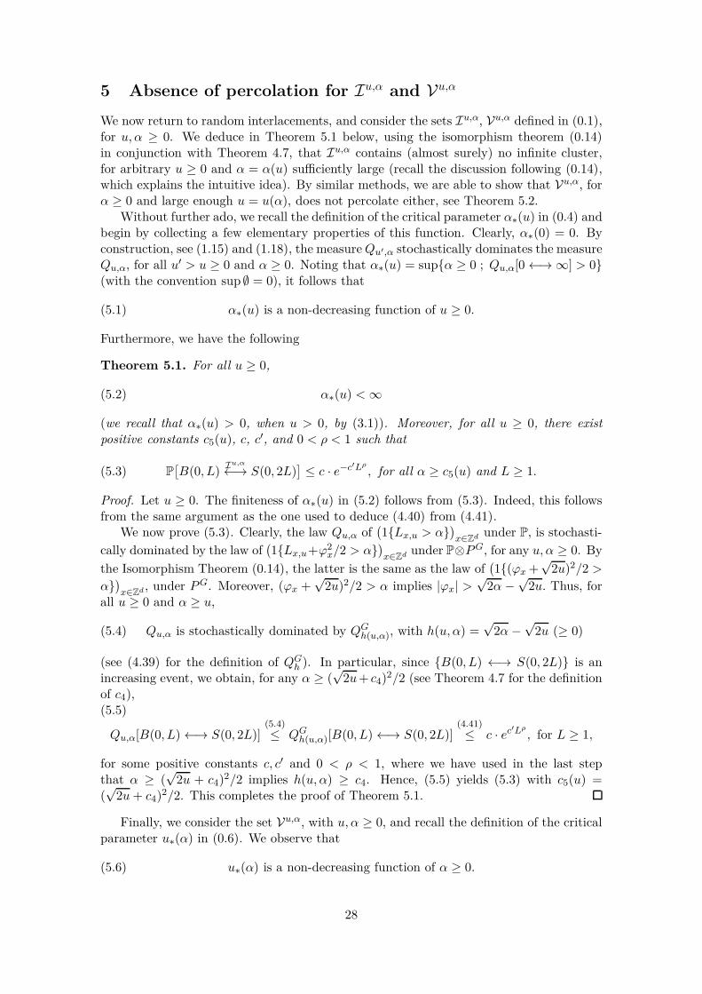
5 Absence of percolation for Iu,α and Vu,α

We now return to random interlacements, and consider the sets Iu,α, Vu,α defined in (0.1),for u, α ≥ 0. We deduce in Theorem 5.1 below, using the isomorphism theorem (0.14)in conjunction with Theorem 4.7, that Iu,α contains (almost surely) no infinite cluster,for arbitrary u ≥ 0 and α = α(u) sufficiently large (recall the discussion following (0.14),which explains the intuitive idea). By similar methods, we are able to show that Vu,α, forα ≥ 0 and large enough u = u(α), does not percolate either, see Theorem 5.2.

Without further ado, we recall the definition of the critical parameter α∗(u) in (0.4) andbegin by collecting a few elementary properties of this function. Clearly, α∗(0) = 0. Byconstruction, see (1.15) and (1.18), the measureQu′,α stochastically dominates the measureQu,α, for all u′ > u ≥ 0 and α ≥ 0. Noting that α∗(u) = supα ≥ 0 ; Qu,α[0←→∞] > 0(with the convention sup ∅ = 0), it follows that

(5.1) α∗(u) is a non-decreasing function of u ≥ 0.

Furthermore, we have the following

Theorem 5.1. For all u ≥ 0,

(5.2) α∗(u) <∞

(we recall that α∗(u) > 0, when u > 0, by (3.1)). Moreover, for all u ≥ 0, there exist

positive constants c5(u), c, c′, and 0 < ρ < 1 such that

(5.3) P[B(0, L)

Iu,α

←→ S(0, 2L)] ≤ c · e−c′Lρ

, for all α ≥ c5(u) and L ≥ 1.

Proof. Let u ≥ 0. The finiteness of α∗(u) in (5.2) follows from (5.3). Indeed, this followsfrom the same argument as the one used to deduce (4.40) from (4.41).

We now prove (5.3). Clearly, the law Qu,α of(1Lx,u > α)

x∈Zd under P, is stochasti-

cally dominated by the law of(1Lx,u+ϕ2

x/2 > α)x∈Zd under P⊗PG, for any u, α ≥ 0. By

the Isomorphism Theorem (0.14), the latter is the same as the law of(1(ϕx +

√2u)2/2 >

α)x∈Zd , under PG. Moreover, (ϕx +

√2u)2/2 > α implies |ϕx| >

√2α −

√2u. Thus, for

all u ≥ 0 and α ≥ u,

(5.4) Qu,α is stochastically dominated by QGh(u,α), with h(u, α) =

√2α−

√2u (≥ 0)

(see (4.39) for the definition of QGh ). In particular, since B(0, L) ←→ S(0, 2L) is an

increasing event, we obtain, for any α ≥ (√

2u+ c4)2/2 (see Theorem 4.7 for the definitionof c4),(5.5)

Qu,α[B(0, L)←→ S(0, 2L)](5.4)

≤ QGh(u,α)[B(0, L)←→ S(0, 2L)]

(4.41)

≤ c · ec′Lρ

, for L ≥ 1,

for some positive constants c, c′ and 0 < ρ < 1, where we have used in the last stepthat α ≥ (

√2u + c4)2/2 implies h(u, α) ≥ c4. Hence, (5.5) yields (5.3) with c5(u) =

(√

2u+ c4)2/2. This completes the proof of Theorem 5.1.

Finally, we consider the set Vu,α, with u, α ≥ 0, and recall the definition of the criticalparameter u∗(α) in (0.6). We observe that

(5.6) u∗(α) is a non-decreasing function of α ≥ 0.

28

Indeed, Vu,α′(ω) ⊃ Vu,α(ω), for all u ≥ 0, α′ > α ≥ 0 and ω ∈ Ω (the space on which

P is defined, see below (1.8)), thus P[0

Vu,α′

←→ ∞] ≥ P[0

Vu,α

←→ ∞], which yields (5.6) since

u∗(α) = supu ≥ 0; P

[0

Vu,α

←→∞]> 0

.

We also note that, since Vu,0 = x ∈ Zd; Lx,u = 0 coincides with the vacant set Vu

of random interlacement at level u introduced in [14], we have u∗(0) = u∗, where u∗ refersto the critical parameter for percolation of Vu. As mentioned in the introduction (see thereferences below (0.6)), u∗ is known to be strictly positive (and finite) for all d ≥ 3. Wenow prove that the set Vu,α undergoes a non-trivial percolation phase transition as u ≥ 0varies, for every (fixed) value of α ≥ 0.

Theorem 5.2. For all α ≥ 0,

(5.7) (0 <) u∗ = u∗(0) ≤ u∗(α) <∞.

Moreover, for all α ≥ 0, there exist positive constants c6(α), c , c′ and 0 < ρ < 1 such

that for all u ≥ c6(α) and all L ≥ 1,

(5.8) P[B(0, L)

Vu,α

←→ S(0, 2L)] ≤ ce−c′Lρ

.

Proof. We begin with (5.7). The inequality u∗(α) ≥ u∗ for all α ≥ 0 is immediate from(5.6) and u∗(0) = u∗. The finiteness of u∗(α) follows from (5.8) (just as (5.3) implies (5.2),see the proof of Theorem 5.1).

It thus remains to show (5.8). The proof encompasses a renormalization argument.Thus, we consider the increasing sequence of length scales (Ln)n≥0 defined in (4.1) (andcorresponding lattices Ln, for n ≥ 0, see (4.2)), with

(5.9) L0 = 10, r = c3(3) and l0 = 2r (see (4.28) for the definition of c3(N)).

In what follows, we identify any event A occurring under P with the event A×RZd

occurringunder P⊗PG, and similarly any event B under PG with Ω×B. For α, u ≥ 0 and x ∈ L0,we define the events (under P⊗ PG)

B(1)0,x(u) =

max

y∈B0,x

ϕy ≥√u/2

,

B(2)0,x(u) =

min

y∈B0,x

ϕy ≤ −√u/2

B(3)0,x(α, u) =

min

y∈B0,x

(Ly,u +

1

2ϕ2

y

)<

1

2

(√2α+

√u/2

)2(5.10)

(see (4.3) for the definition of the boxes B0,x). We call a vertex x ∈ L0 (α, u)-bad if

(5.11) B(1)0,x(u) ∪ B(2)

0,x(u) ∪ B(3)0,x(α, u)

occurs under P⊗ PG. The reason for the choices in (5.10) is the following

Lemma 5.3. (u, α ≥ 0)

For all n ≥ 0 and x ∈ Ln,

(5.12) P[B(x,Ln)

Vu,α

←→ S(x, 2Ln)] ≤ P⊗ PG[

B(x,Ln)(α,u)-bad←→ S(x, 2Ln)

],

whereB(x,Ln)

(α,u)-bad←→ S(x, 2Ln)

is the event that there exists a nearest-neighbor path

of (α, u)-bad vertices in L0 connecting B(x,Ln) ∩ L0 to S(x, 2Ln) ∩ L0.

29

Proof of Lemma 5.3. By translation invariance, it suffices to consider the case x = 0. Let

n ≥ 0. By definition, ifB(0, Ln)

Vu,α

←→ S(0, 2Ln)

occurs, there exists a nearest-neighborpath π of vertices in Vu,α connecting B(0, Ln) to S(0, 2Ln). We consider π0, the trace ofπ on L0, see (4.4), and show that

(5.13) all vertices traversed by π0 are (α, u)-bad.

This implies (5.12), for by construction (cf. (4.5)), π0 is a nearest-neighbor path in L0

connecting B(0, Ln) ∩ L0 to S(0, 2Ln) ∩ L0, whenceB(0, Ln)

Vu,α

←→ S(0, 2Ln) × R

Zd ⊆

B(0, Ln)

(α,u)-bad←→ S(0, 2Ln), which yields (5.12).

Let x ∈ L0 be any vertex in range(π0). By definition of π0, B0,x∩π 6= ∅. In particular,

(5.14) Ly0 ≤ α, for some y0 ∈ B0,x.

We now assume B(3)0,x(α, u) does not occur, i.e. Ly,u + ϕ2

y/2 ≥(√

2α +√u/2

)2/2, for all

y ∈ B0,x. Then,

α+1

2ϕ2

y0

(5.14)≥ Ly0 +

1

2ϕ2

y0≥ 1

2

(√2α+

√u/2

)2 ≥ α+u

4,

i.e. ϕ2y0≥ u/2, where we have used (a + b)2 ≥ a2 + b2 for all a, b ≥ 0 in the last step.

Thus, B(1)0,x(u) ∪ B(2)

0,x(u) = maxy∈B0,x|ϕy| ≥

√u/2 occurs, and therefore x is (α, u)-bad.

This completes the proof of (5.13), and thus of Lemma 5.3.

We now return to the proof of (5.8), and define the events B(1)n,x(u), B(2)

n,x(u), B(3)n,x(α, u),

for n ≥ 0, x ∈ Ln, and u, α ≥ 0, by

B(1)n,x(u) =

⋃

T ∈Λn,x

⋂

m∈T (n)

B(1)0,T (m)(u),

and similarly for B(2)n,x(u), B(3)

n,x(α, u). As in (4.46), when i = 1 or 2, we obtain, using (5.10),(4.8) and the symmetry of PG,

(5.15) P⊗ PG[B(i)n,x(u)] ≤ (

l2d0

)2n

· pAn

(√u/2

), for all n ≥ 0, x ∈ Ln, u ≥ 0,

where A refers to the family of events (on 0, 1Zd

) defined in (4.18) and pAn (·) is given by

(4.11). As for the third collection of events, we claim that

(5.16) P⊗ PG[B(3)n,x(α, u)] ≤ (

l2d0

)2n

· pAn

(√u/2 −

√2α

), for all n ≥ 0, x ∈ Ln, u, α ≥ 0.

Indeed, the Isomorphism Theorem (0.14) applied to the events B(3)0,x(α, u) from (5.10) yields

P⊗ PG[B(3)n,x(α, u)] ≤ |Λn,x| · sup

T ∈Λn,x

P⊗ PG[ ⋂

m∈T (n)

B(3)0,T (m)(α, u)

]

(0.14)= |Λn,x| · sup

T ∈Λn,x

PG[ ⋂

m∈T (n)

min

y∈B0,T (m)

∣∣ϕy +√

2u∣∣ <√

2α+√u/2

]

≤ |Λn,x| · supT ∈Λn,x

PG[ ⋂

m∈T (n)

min

y∈B0,T (m)

ϕy <√

2α−√u/2

],

which, using (4.8) to bound |Λn,x| and symmetry of PG, yields (5.16).Since K0 as defined in (4.22) is fully determined by the choice of l0 in (5.9), the BTIS-

inequality yields (cf. the argument leading to (4.48)) pA0 (h) ≤ e−K0 , for all h ≥ c. The

30

sequence (hn)n≥0 defined in (4.23) with h0 = c (and L0, l0, r given by (5.9)) has a finitelimit h∞ = limn→∞ hn, see (4.24), and Proposition 4.3 implies that pA

n (h∞) ≤ (2l2d0 )−2n

,for all n ≥ 0, cf. (4.49). Together with (5.15), (5.16), and setting

√u∞(α)/2 =

√2α+h∞,

this yields

P⊗ PG[B(1)n,x(u∞(α))] = P⊗ PG[B(2)

n,x(u∞(α))](5.15),(4.17)

≤ 2−2n

P⊗ PG[B(3)n,x(α, u∞(α))]

(5.16)

≤ 2−2n

,

(5.17)

for all n ≥ 0, x ∈ Ln and α ≥ 0. On account of (5.17) and the choice of r in (5.9),

Lemma 4.5 applies (with N = 3, P = P⊗ PG, ζ(1)x = 1ϕx ≥

√u∞(α)/2, ζ(2)

x = 1ϕx ≤−

√u∞(α)/2 and ζ

(3)x = 1Ly,u∞(α) +ϕ2

y/2 <(√

2α+√u∞(α)/2

)2/2, x ∈ Z

d, see (4.27)and (5.10)), and we obtain, using Lemma 5.3, that for all n ≥ 0, x ∈ Ln, α ≥ 0 andu ≥ u∞(α)(5.18)

P[B(x,Ln)

Vu,α

←→ S(x, 2Ln)] ≤ P

[B(x,Ln)

Vu∞(α),α

←→ S(x, 2Ln)]

(5.12)

≤ P⊗ PG[B(x,Ln)

(α,u∞(α))-bad←→ S(x, 2Ln)]

(5.11),(4.38)≤ c2−2n

,

(where we also used in the first line that the law Qu,α of (1x ∈ Vu,α)x∈Zd , is stochasticallydominated by Qu′,α, for all u ≥ u′). By the same interpolation argument as that in

(4.52), we deduce from (5.18) that P[B(0, L)

Vu,α

←→ S(0, 2L)] ≤ ce−c′Lρ

, for some c, c′ > 0,ρ = log 2/ log l0 and all u ≥ u∞(α). Hence, (5.8) holds with c6(α) = u∞(α). Thiscompletes the proof of Theorem 5.2.

Remark 5.4. 1) From (5.3) and (5.8), one easily deduces that the connectivity functions

P[0

Iu,α

←→ x], P

[0

Vu,α

←→ x]

have stretched exponential decay in x as |x| → ∞, for all u ≥ 0and α ≥ c5(u), respectively for all α ≥ 0 and u ≥ c6(α) (cf. Remark 4.8, 1)).

2) One may introduce the auxiliary critical parameters (cf. Figure 1 in Section 0)

u∗∗(α) = infu ≥ 0; P

[B(0, L)

Vu,α

←→ S(0, 2L)]

has stretched exponential decay in L,

and similarly α∗∗(u), where the infimum is now over all α ≥ 0 and the event in the

probability is replaced byB(0, L)

Iu,α

←→ S(0, 2L)

(note in particular that u∗∗(0) coincideswith the quantity u∗∗ from [12]). Theorems 5.1 and 5.2 imply that α∗(u) ≤ α∗∗(u) < ∞for all u ≥ 0 and u∗(α) ≤ u∗∗(α) < ∞ for all α ≥ 0. This raises the important questionwhether the parameters actually coincide.

Acknowledgement. The author wishes to thank his advisor A.-S. Sznitman for sug-gesting the problem and for useful discussions, and the anonymous referee for valuablecomments.

References

[1] R. J. Adler and J. E. Taylor. Random fields and geometry. Springer, New York(2007).

31

[2] J. Bricmont, J. L. Lebowitz and C. Maes. Percolation in strongly correlated systems:the massless Gaussian field. J. Stat. Phys., 48(5/6): pp. 1249-1268 (1987).

[3] M. T. Barlow and J.-D. Deuschel. Invariance principle for the random conductancemodel with unbounded conductances. Ann. Prob., 38(1): pp. 234-276 (2010).

[4] R. M. Burton and M. Keane. Density and uniqueness in percolation. Commun. Math.

Phys., 121(3): pp. 501-505 (1989).

[5] M. Disertori, T. Spencer and M. R. Zirnbauer. Quasi-diffusion in a 3D supersym-metric hyperbolic sigma model. Commun. Math. Phys., 300: pp. 435-486 (2010).

[6] M. Disertori and T. Spencer. Anderson localization for a supersymmetric sigmamodel. Commun. Math. Phys., 300: pp. 659-671 (2010).

[7] O. Garet. Percolation transition for some excursion sets. Elec. J. Prob., 9(paper no.10): pp. 255-292 (2004).

[8] O. Haggstrom and J. Jonasson. Uniqueness and non-uniqueness in percolation the-ory. Probab. Surv. 3: pp. 289-344 (2006).

[9] B. Rath and A. Sapozhnikov. The effect of small quenched noise on connectivityproperties of random interlacements. Elec. J. Prob., 18(paper no. 4): pp. 1-20 (2013).

[10] S. I. Resnick. Extreme values, regular variation and point processes. Springer, NewYork (1987).

[11] P.-F. Rodriguez and A.-S. Sznitman. Phase transition and level-set percolation forthe Gaussian free field. To appear in Commun. Math. Phys.

[12] V. Sidoravicius and A.-S. Sznitman. Connectivity bounds for the vacant set of ran-dom interlacements. Ann. Inst. Henri Poincare, Probabilites et Statistiques, 46(4):pp. 976-990 (2010).

[13] V. Sidoravicius and A.-S. Sznitman. Percolation for the vacant set of random inter-lacements. Comm. Pure Appl. Math. 62(6): pp. 831-858 (2009).

[14] A.S. Sznitman. Vacant set of random interlacements and percolation. Ann.

Math. 171: pp. 2039-2087 (2010).

[15] A. S. Sznitman. An isomorphism theorem for random interlacements. Electron. Com-

mun. Probab. 17(9): pp. 1-9 (2012).

[16] A.S. Sznitman. Decoupling inequalities and interlacement percolation on G × Z.Inventiones mathematicae, 187: pp. 645-706 (2012).

[17] A. Teixeira. On the uniqueness of the infinite cluster of the vacant set of randominterlacements. Ann. Appl. Prob. 19(1): pp. 454-466 (2009).

32