CloudSat Project

A NASA Earth System Science Pathfinder Mission

Level 2 Cloud Optical Depth Product Process Description and Interface

Control Document

Version: 5.0

Date: February 20, 2008

Questions concerning the document and proposed changes shall be addressed to

Igor N. Polonsky: polonsky@atmos.colostate.edu

Laurent C. Labonnote: laurent@atmos.colostate.edu

Steve Cooper: cooper@atmos.colostate.edu

Cooperative Institute for Research in the Atmosphere

Colorado State University

Fort Collins, CO 80523

Contents 1 Introduction 3

1.1 Purpose 3

2 Basis of the Algorithm 3

2.1 Overview 3

2.2 Forward Radiative Transfer Model 4

2.2.1 Theory 4

2.2.2 Method of Solution 5

2.2.3 Implementation 6

2.3 Bayesian Retrieval 6

2.3.1 a priori Estimates 7

2.3.2 MODIS Reflectivity and Uncertainties 7

2.3.3 Iteration and Convergence 7

3 Algorithm Inputs 9

3.1 CloudSat 9

3.1.1 CloudSat Level2B Geometric Profile 9

3.2 Ancillary (Non-CloudSat) 10

3.2.1 CloudSat Ancillary Albedo Dataset 10

3.2.2 CloudSat Auxiliary MODIS Reflectivity 10

3.2.3 CloudSat Auxiliary ECMWF Dataset 11

3.3 Control and Calibration 11

4 Algorithm Implementation 11

4.1 Flowchart overview of the retrieval algorithm 11

4.2 Pseudo code description 13

4.2.1 Algorithm Parameters 16

4.3 Timing Requirements 16

5 Data Product Output Format 17

5.1 Data Contents 17

5.2 Data Format Overview 17

5.3 Data Descriptions 18

6 Operator Instructions 20

7 Acronym List 20

1 Introduction

This document provides an overview of the 2B-TAU cloud optical depth retrieval algorithm. The document

describes the algorithm's:

• purpose,

• scientific basis,

• required inputs,

• implementation,

• outputs, and

• operator instructions.

1.1 Purpose

The primary objective of the algorithm is to produce estimates of the optical depth (τ) and its

uncertainty for each radar profile determined to contain cloud. However, as shown below, to obtain

accurate estimates of optical depth, τ , the effective radius, , must be retrieved as well (Breon et al.[1]).

To appreciate the importance of retrieving , Fig. 1a and 1b illustrate the consequences of assuming an

incorrect asymmetry factor on the retrieved optical depth.

effr

effr

MODIS reflectivities depend upon the observational geometry (observational, θ , and solar

zenith, 0θ , angles, azimuthal angle difference, 0φ φ− ) according to the geographical position of AQUA

satellite. Although these angles range from nadir to about 20o, retrievals performed at nadir would be

calculated at higher speed, but would incur intolerably large errors as shown in Fg 1c. The selected

algorithm allows for arbitrary viewing angles. The optical depth and effective radius are retrieved using

upwelling reflectivity at the top of the atmosphere (TOA) measured by MODIS in several channels and

other ancillary data (e.g., geolocation, meteorological parameters and surface albedo). The retrieved values

are spectral and represent the optical depth and effective radius at the short wave. The radar reflectivity

measured by the CloudSat Profiling Radar (CPR) provides information about the cloud distribution in the

atmospheric column, and serves as a quantitative basis to produce cloud optical depth profiles.

2 Basis of the Algorithm

2.1 Overview

The retrieval uses a Bayesian statistical approach described by Marks and Rogers [2]. The

retrieved state vector containing the optical depth and effective radius is obtained by using the MODIS

reflectivity measurements to refine a priori information and also subjects to the uncertainties in both the a

priori information and the measurement uncertainties. The CPR reflectivity is used to produce the a priori

value of τ and its associated uncertainty. Another fundamental component is a forward model which

provides us with the simulated TOA reflectivities for the atmospheric model described by the state vector.

Comparison between the simulated and measured TOA reflectivities is used to update the state vector and

allows us to converge iteratively to a solution. The forward model uses a multi-stream plane-parallel adding

model (Christi and Gabriel [3]) based on methods by Benedetti et al. [4]. The next subsection contains a

brief description of the retrieval algorithm components.

Fig. 1: a) Retrieved optical depth for different asymmetry factors (colored lines). True asymmetry factor is

g=0.85. b) As in a) except that errors are shown. c) Error on retrieved optical depth due to incorrect

observation angle. True exiting reflectivities at indicated angles are shown by colored lines. Retrieved

optical depths computed at Nadir

2.2 Forward Radiative Transfer Model

2.2.1 Theory

The model used here incorporates a cloud layer overlying a reflecting surface. The optical

properties of the cloud and surface are assumed to be horizontally homogeneous. In addition, the optical

properties of the cloud are assumed to be vertically homogeneous. Given these assumptions the

monochromatic 1D radiative transfer equation (RTE):

2 1

0 1

( , , ) ( , , ) ( , ; ', ') ( , ', ') ' ' ( , , ),4

dI I P I d d Sd

πτ μ φ ωμ τ μ φ μ φ μ φ τ μ φ μ φ τ μ φτ π −

= − + +∫ ∫ (2.1)

where ( , , )I τ μ φ is the radiance observed at a height expressed by the optical depth τ in the direction given

by cos( )μ θ= and φ , ω is the single scattering albedo, which is measure of the degree of absorption and

spans the range between 1 and 0, with 1 and 0 meaning purely scattering and purely absorbing media,

correspondingly, ( ,P ; ', ')μ φ μ φ is the phase function and represents the angular pattern of the scattered

radiation.

The source term in Eq. (2.1) has a form

0 0 0 0( , , ) ( , ; , ) exp( / ) (1 ) ( ),4

S F Pωτ μ φ μ φ μ φ τ μ ωπ

= − + B T− (2.2)

where 0F is the monochromatic solar flux at the top of the atmosphere, 0 cos( )0μ θ= , 0θ and 0φ are the

zenith and azimuth angles at which the solar radiance illuminates the top of the atmosphere. The second

term of the source function, ( , , )S τ μ φ , represents the contributions of longwave radiation which can be

described by the Planck function. Since 2B-TAU algorithm uses MODIS reflectivities, we can set 0F π= .

The solution of (2.1) is subject to the standard boundary conditions. They describe radiance

interaction with the surface at the bottom of the atmosphere.

2.2.2 Method of solution of the RTE

The selected algorithm uses a multi-stream plane-parallel adding model. This method is based on a

discretization of the equation of transfer so that the Eq. (2.1) is represented in a discrete ordinate form and

then the adding method is applied to obtain the solution. We decompose ( , ', ')I τ μ φ , and ( , , )S τ μ φ over the

azimuthal coordinate φ using Fourier series. The functions are decomposed over the zenith coordinate μ

using numerical quadrature (i.e. Gaussian). The phase function ( ,P ; ', ')μ φ μ φ is represented as a series of

the Legendre polynomials. Our model assumes that clouds can be represented as plane-parallel entities

comprised of water or ice, and hence, our atmosphere can be divided into homogeneous layers. In this case,

the radiances can be calculated by employing the interaction principle repeatedly to all layers resulting in a

variation of the well known adding method. The global reflection, transmission matrices and source

functions required by the adding method are calculated using an eigenmatrix technique described in [3],[4].

This method differs from the doubling method in that the global operators (i.e. the reflection ( ) and

transmission (T ) matrices) also used in the construction of the source functions can be computed for any

optical depth directly using formulas that do not require iteration. By contrast, doubling procedure is

initialized by an infinitesimal generator and uses thereafter repeated matrix-to-matrix multiplications to

R

calculate the global operator associated with a given optical depth. As demonstrated by Cristi and Gabriel

[3] this method is computationally efficient and stable.

2.2.3 Implementation details:

The forward model is implemented as follows:

1. Because of the solar radiance is a directional source and any value of the observation and solar

illumination angles is possible, it may be required to take into account several azimuthal

harmonics to achieve a required accuracy of the radiance estimation. This number generally

increases when the observation and solar illumination angles become larger. Our numerical

experiment shows that four harmonics are enough for most cloud scenes.

2. For the far infrared channels (wavelength grater than 3 μm), since the thermal sources are

angularly isotropic, only the zeros azimuth harmonic is required regardless of the observation

geometry.

3. The expansion over μ uses 8 angles up and 8 angles down. Correspondingly, the number of the

expansion terms in the Legendre polynomial decomposition of the phase function is set to 16.

4. The measurement of the TOA reflectivities at two wavelengths to infer both τ and efr is

necessary.

5. A Lambertian surface is assumed. The surface albedo depends on geographical location and the

day of the year and obtained from a datafile.

6. The phase function dependents on the cloud constituent type. For the liquid water cloud, we

assume that cloud particles have the spherical shape and their size distribution, ( )p r , is described

by the gamma distribution

1 exp( / )( )( )

kk

r bp r rk b

− −=

Γ, (2.3)

where is the Gamma function. ( )kΓ

For the ice water cloud the model suggested by Yang et al [5] is used.

7. The single scattering albedo and coefficients of phase function decomposition into the Legendre

polynomials are pre-calculated and organized as look up tables.

2.3 Bayesian Retrieval

The general approach of the retrieval is as shown in Figure 2, starting with process 5 (Estimate

priorx ) and ending with process 8 (Eval QC flags). In general, for each cloudy profile produced by the CPR,

an a priori estimate of the column vector containing cloud optical and effective radius is supplied. The

estimates are updated until the forward-modeled reflectivities produced by the estimates are in agreement

with the observed reflectivities obtained from MODIS, subject to the uncertainties in both the a priori

estimates and in the MODIS reflectivities.

2.3.1 a priori Estimates

Initial estimates (a priori estimates) of column cloud optical depth and effective radius are required for the

retrieval. If the CPR indicates the column is cloudy, the radar reflectivity profile is used to produce the a

priori estimate. Each radar range gate is assumed to hold liquid or ice exclusively. Using a fixed

temperature defining the phase transition (253 K), the ECMWF-AUX temperature profile is used to

determine the water phase contained in each range gate. The auxiliary datasets (IWC-RO-AUX and CWC-

RO-AUX) are used to provide information about the liquid/ice water contents for the each range gate. The

water contents are then converted to the optical depths using the anomalous diffraction theory (Mitchell and

Arnott [6]). The effective radius is the same as that used in the CPR to obtain the optical depth.

If a column is indicated cloudy by the MODIS scene characterization obtained from 2B-GEOPROF but

the CPR does not indicate cloud, the a priori optical depth and effective radius are estimated by decoding

the MODIS scene characterization and assigning the values which are typical to the characterization.

2.3.2 MODIS Reflectivities and Uncertainties

A subset of MODIS reflectivities and uncertainties are obtained from the MODIS level 1B

radiance product. The subset consists of a 3x5 grid of MODIS pixels for each CloudSat profile. A vector of

MODIS reflectivities values (0.864 μm and 2.13 μm for day time retrieval; 3.7 μm and 11.0 μm for night

time retrieval) and a vector of reflectivity uncertainties are associated with each pixel. For each CloudSat

profile, a simple mean is taken of the valid reflectivity and uncertainty values over this 3x5 grid.

2.3.3 Iteration and Convergence

The framework for iteratively updating the state vector x containing the cloud optical depth and

effective radius and testing for convergence is similar to that described by Marks and Rodgers [2] and by

Rogers [7]. The expression for the updated value of x is given by (adapted from Eq. (5.9) of Rodgers [7])

is:

1 1 1 11 [ ] [ ( ) (T T

i i a i e i i e e i i i a )]x x I I x− − − −+ = + + − + −S K S K K S K x x , (2.4)

where the subscript refers to a priori values, the subscript refers to the measured values, and the

subscripts refer to the iteration cycle number. In Eq.

a e

,i i +1 (2.4) x is the column state vector containing

the optical depth and effective radius, and K is the Jacobian matrix:

1 1

2 2

eff

eff

dI dId dr

dI dId dr

λ λ

λ λ

τ

τ

⎛ ⎞⎜ ⎟⎜ ⎟⎜=⎜ ⎟⎜ ⎟⎜ ⎟⎝ ⎠

K ⎟ (2.5)

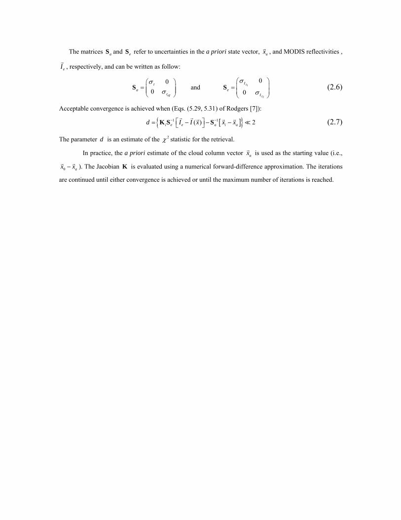
The matrices and refer to uncertainties in the a priori state vector, aS eS ax , and MODIS reflectivities ,

eI , respectively, and can be written as follow:

(2.6) 1

2

00and0 0

eff

I

a er I

λ

λ

τσσ

σ σ

⎛ ⎞⎛ ⎞⎜= ⎜ ⎟⎜ ⎟ ⎜⎝ ⎠ ⎝ ⎠

S S ⎟=⎟

}Acceptable convergence is achieved when (Eqs. (5.29, 5.31) of Rodgers [7]):

[ ]{ 1 1( ) 2i e e a i ad I I x x x− −⎡ ⎤= − − −⎣ ⎦K S S (2.7)

The parameter is an estimate of the d 2χ statistic for the retrieval.

In practice, the a priori estimate of the cloud column vector ax is used as the starting value (i.e.,

0 ax x− ). The Jacobian is evaluated using a numerical forward-difference approximation. The iterations

are continued until either convergence is achieved or until the maximum number of iterations is reached.

K

3 Algorithm Inputs

3.1 CloudSat

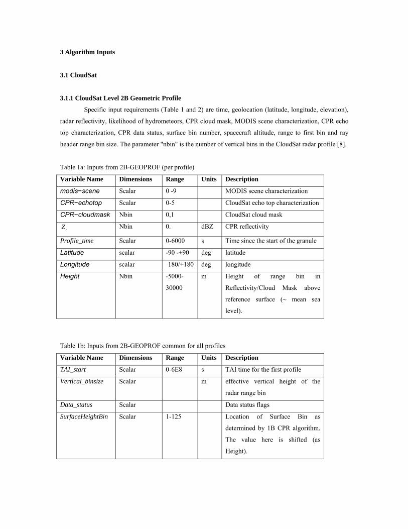
3.1.1 CloudSat Level 2B Geometric Profile

Specific input requirements (Table 1 and 2) are time, geolocation (latitude, longitude, elevation),

radar reflectivity, likelihood of hydrometeors, CPR cloud mask, MODIS scene characterization, CPR echo

top characterization, CPR data status, surface bin number, spacecraft altitude, range to first bin and ray

header range bin size. The parameter "nbin" is the number of vertical bins in the CloudSat radar profile [8].

Table 1a: Inputs from 2B-GEOPROF (per profile)

Variable Name Dimensions Range Units Description

modis−scene Scalar 0 -9 MODIS scene characterization

CPR−echotop Scalar 0-5 CloudSat echo top characterization

CPR−cloudmask Nbin 0,1 CloudSat cloud mask

rZ Nbin 0. dBZ CPR reflectivity

Profile_time Scalar 0-6000 s Time since the start of the granule

Latitude scalar -90 -+90 deg latitude

Longitude scalar -180/+180 deg longitude

Height Nbin -5000-

30000

m Height of range bin in

Reflectivity/Cloud Mask above

reference surface (~ mean sea

level).

Table 1b: Inputs from 2B-GEOPROF common for all profiles

Variable Name Dimensions Range Units Description

TAI_start Scalar 0-6E8 s TAI time for the first profile

Vertical_binsize Scalar m effective vertical height of the

radar range bin

Data_status Scalar Data status flags

SurfaceHeightBin Scalar 1-125 Location of Surface Bin as

determined by 1B CPR algorithm.

The value here is shifted (as

Height).

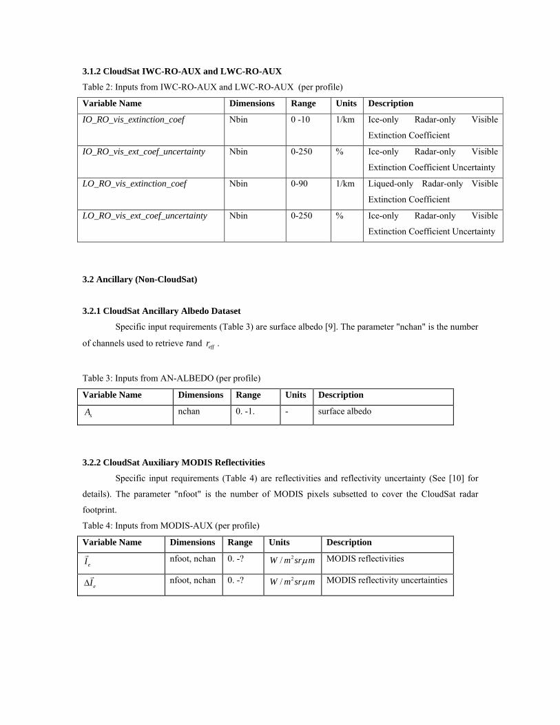
3.1.2 CloudSat IWC-RO-AUX and LWC-RO-AUX

Table 2: Inputs from IWC-RO-AUX and LWC-RO-AUX (per profile)

Variable Name Dimensions Range Units Description

IO_RO_vis_extinction_coef Nbin 0 -10 1/km Ice-only Radar-only Visible

Extinction Coefficient

IO_RO_vis_ext_coef_uncertainty Nbin 0-250 % Ice-only Radar-only Visible

Extinction Coefficient Uncertainty

LO_RO_vis_extinction_coef Nbin 0-90 1/km Liqued-only Radar-only Visible

Extinction Coefficient

LO_RO_vis_ext_coef_uncertainty Nbin 0-250 % Ice-only Radar-only Visible

Extinction Coefficient Uncertainty

3.2 Ancillary (Non-CloudSat)

3.2.1 CloudSat Ancillary Albedo Dataset

Specific input requirements (Table 3) are surface albedo [9]. The parameter "nchan" is the number

of channels used to retrieve τand . effr

Table 3: Inputs from AN-ALBEDO (per profile)

Variable Name Dimensions Range Units Description

sA nchan 0. -1. - surface albedo

3.2.2 CloudSat Auxiliary MODIS Reflectivities

Specific input requirements (Table 4) are reflectivities and reflectivity uncertainty (See [10] for

details). The parameter "nfoot" is the number of MODIS pixels subsetted to cover the CloudSat radar

footprint.

Table 4: Inputs from MODIS-AUX (per profile)

Variable Name Dimensions Range Units Description

eI nfoot, nchan 0. -? 2/W m sr mμ MODIS reflectivities

eIΔ nfoot, nchan 0. -? 2/W m sr mμ MODIS reflectivity uncertainties

3.2.3 CloudSat Auxiliary ECMWF Dataset

Specific input requirements (Table 5) are the temperature, specific humidity, and pressure profile

as well as surface temperature and pressure. See [9].

Table 5: Inputs from ECMWF-AUX (per profile)

Variable Name Dimensions Range Units Description

T nbin 0. -? K temperature profile

P nbin 0. -? Pa pressure profile

uS nbin 0. -? Kg/Kg Specific humidity

0P scalar 0. -? Pa surface pressure

0T scalar 0. -? K surface temperature

3.3 Control and Calibration

TBD by 2B-TAU algorithm team.

4 Algorithm Implementation

4.1 Flowchart overview of the retrieval algorithm

See Figure 2.

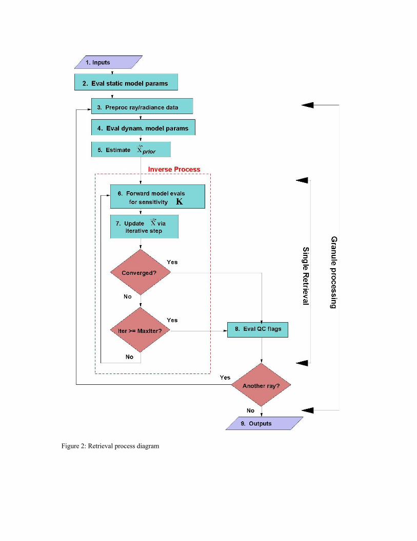
Figure 2: Retrieval process diagram

4.2 Pseudocode description

Following is a pseudocode description of the algorithm: start 2B-TAU

open (2B-GEOPROF, 1B-CPR)

open ancillary data files (AN-ALBEDO, MODIS-AUX, ECMWF-AUX)

set TOA 0F π=

get (solar, sensor) zenith angle (SZA,SEZA) (MODIS-AUX)

get (solar, sensor) azimuth angle (SAA,SEAA) (MODIS-AUX)

for-each 2B-GEOPROF profile

clear status

if ( ) OR ( ) perform the retrieval maxSZA SZA≤ horizSZA SZA>

set status: daytime or nighttime

read MODIS scene characterization (2B-GEOPROF)

read CPR echo top characterization (2B-GEOPROF)

eval status:scene

if status:scene=not clear

compute relative azimuth angle

read CPR reflectivity profile

read CPR cloud mask (2B-GEOPROF)

read ECMWF (temperature, pressure, specific humidity and

ozone) (ECMWF-AUX)

compute gas absorption (correlated-k distribution)

eval status:phase

set prior effective radius (from cloud phase information)

and uncertainty

read surface albedo(AN-ALBEDO)

read MODIS reflectivity data (MODIS-AUX)

compute spatially-averaged MODIS reflectivity vector

read prior optical thickness (IWC-RO-AUX and LWC-RO-AUX)

compute ax and aS

set convergence parameter to the initial value d

set iteration counter 0i =

set i ax x=

while ( and 1d > maxi i< )

compute ( )iI x

compute ( )i iI τ δτ+

compute , ,( )eff i eff iI r rδ+

compute aK

compute ix

compute d

set i i 1= +

end-wh and ile ( 1d > maxi i< )

fail con ge)

set

if maxi i== ( ed to ver

τ =flagmissing

set ( )binτ =flagmissing

f set lagmissing effr =

set τσ =flagmissing

set effrσ =flagmissing

set flagmissing d =

set s atus:no_convert ge

se

set

el

iτ τ=

comput e τσ (uncertainty in retrieved optical depth)

compute effr

compute effrσ (uncertainty in retrieved effective

mpute

radius)

co ( )binτ vertical profile of cloud optical

pth) de

set id d=

set s s:tatu converge, status:prior

d-if en ( maxi i== )

else (s ne=clear) tatus:sce

set τ = flagclear

set ( )binτ = flagclear

set flagclear effr =

set τσ = flagclear

set effrσ = flagclear

set flagclear d =

en (status:scene = nod-if t clear)

else ( maxSZA SZA> ) OR ( horizSZA SZA< ) no retrieval

set τ =flagmissing

set ( )binτ =flagmissing

set lagmissing effr =f

set τσ =flagmissing

set effrσ =flagmissing

set flagmissing d =

end-if (SZA<SZAmax

end-fo ofile)

)

r-each (2B-GEOPROF pr

compute scaled τ , effr , τσ , effrσ , (bin)τ , and

u fi

d

open 2B-TAU outp t le

write status, scaled τ , r , τσ , effrσ , ( )binτeff , and

l

a files

d

close 2B-TAU output fi e

close 2B-GEOPROF

close ancillary dat

stop 2B-TAU

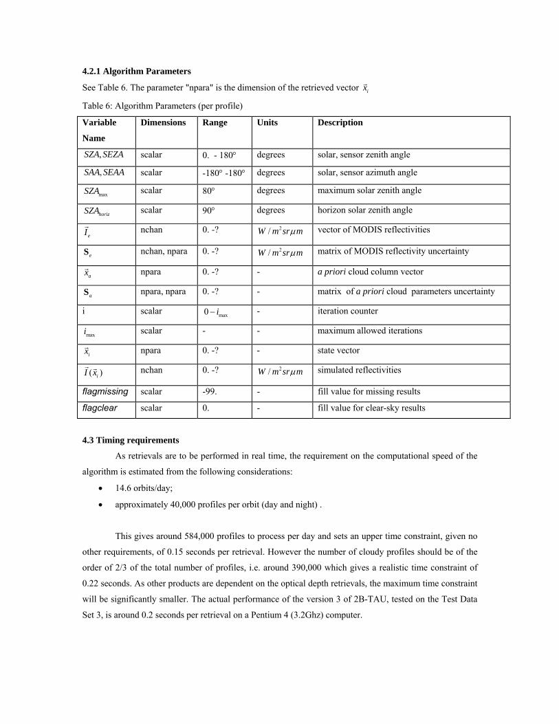
4.2.1 Algorithm Parameters

See Table 6. The parameter "npara" is the dimension of the retrieved vector ix

Table 6: Algorithm Parameters (per profile)

Variable

Name

Dimensions Range Units Description

,SZA SEZA scalar 0. - 180° degrees solar, sensor zenith angle

,SAA SEAA scalar -180° -180° degrees solar, sensor azimuth angle

maxSZA scalar 80° degrees maximum solar zenith angle

horizSZA scalar 90° degrees horizon solar zenith angle

eI nchan 0. -? 2/W m sr mμ vector of MODIS reflectivities

eS nchan, npara 0. -? 2/W m sr mμ matrix of MODIS reflectivity uncertainty

ax npara 0. -? - a priori cloud column vector

aS npara, npara 0. -? - matrix of a priori cloud parameters uncertainty

i scalar max0 i− - iteration counter

maxi scalar - - maximum allowed iterations

ix npara 0. -? - state vector

( )iI x nchan 0. -? 2/W m sr mμ simulated reflectivities

flagmissing scalar -99. - fill value for missing results

flagclear scalar 0. - fill value for clear-sky results

4.3 Timing requirements

As retrievals are to be performed in real time, the requirement on the computational speed of the

algorithm is estimated from the following considerations:

• 14.6 orbits/day;

• approximately 40,000 profiles per orbit (day and night) .

This gives around 584,000 profiles to process per day and sets an upper time constraint, given no

other requirements, of 0.15 seconds per retrieval. However the number of cloudy profiles should be of the

order of 2/3 of the total number of profiles, i.e. around 390,000 which gives a realistic time constraint of

0.22 seconds. As other products are dependent on the optical depth retrievals, the maximum time constraint

will be significantly smaller. The actual performance of the version 3 of 2B-TAU, tested on the Test Data

Set 3, is around 0.2 seconds per retrieval on a Pentium 4 (3.2Ghz) computer.

5 Data Product Output Format

5.1 Data Contents

The data specifically produced by the 2B-TAU algorithm are described in Table 7.

Table 7: Algorithm Outputs (per profile)

Variable Name Dimensions Range Units Description

τ scalar 0 .-200 - total cloud column optical depth

effr scalar 0 .-200 - cloud column effective radius

τσ scalar 0. -200 - scaled standard deviation of τ

effrσ scalar 0. -200 - scaled standard deviation of effr

d scalar 0. -100 - 2χ estimate

( )binτ nbins 0. -200 - distributed column optical depth

status scalar 0 -127 - retrieval mode and status

5.2 Data Format Overview

In addition to the data specific to the 2B-TAU algorithm results, the HDF-EOS data structure may

incorporate granule data/metadata (describing the characteristics of the orbit or granule) and supplementary

ray data/metadata. The data structure is described in Table 8. Only those common data fields specifically

required by the 2B-TAU algorithm are listed in the table and included in the descriptions in section 5.3.

The entries in the "Size" column of the table represent the array size where appropriate (e.g., nray), the

variable type (REAL, INTEGER, CHAR) and the size in bytes of each element (e.g., (4)). The parameter

"nray" is the total number of profiles in the granule.

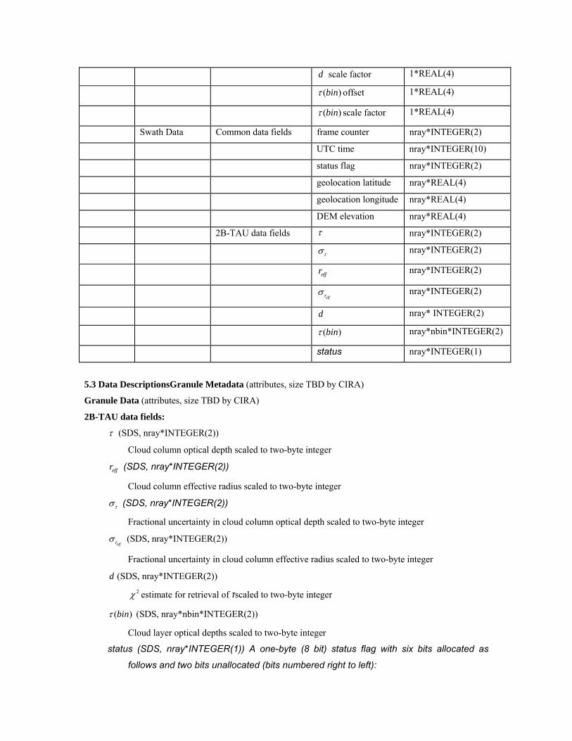
Table 8: HDF-EOS File Structure

Structure/Data Name Size

Data Granule Granule Metadata TBD

Granule Data TBD

Swath Metadata Common metadata TBD TBD

2B-TAU metadata τ offset 1*REAL(4)

τ scale factor 1*REAL(4)

effr offset 1*REAL(4)

effr scale factor 1*REAL(4)

d offset 1*REAL(4)

d scale factor 1*REAL(4)

(bin)τ offset 1*REAL(4)

(bin)τ scale factor 1*REAL(4)

Swath Data Common data fields frame counter nray*INTEGER(2)

UTC time nray*INTEGER(10)

status flag nray*INTEGER(2)

geolocation latitude nray*REAL(4)

geolocation longitude nray*REAL(4)

DEM elevation nray*REAL(4)

2B-TAU data fields τ nray*INTEGER(2)

τσ nray*INTEGER(2)

effr nray*INTEGER(2)

effrσ nray*INTEGER(2)

d nray* INTEGER(2)

( )binτ nray*nbin*INTEGER(2)

status nray*INTEGER(1)

5.3 Data DescriptionsGranule Metadata (attributes, size TBD by CIRA)

Granule Data (attributes, size TBD by CIRA)

2B-TAU data fields:

τ (SDS, nray*INTEGER(2))

Cloud column optical depth scaled to two-byte integer

effr (SDS, nray*INTEGER(2))

Cloud column effective radius scaled to two-byte integer

τσ (SDS, nray*INTEGER(2))

Fractional uncertainty in cloud column optical depth scaled to two-byte integer

effrσ (SDS, nray*INTEGER(2))

Fractional uncertainty in cloud column effective radius scaled to two-byte integer

d (SDS, nray*INTEGER(2)) 2χ estimate for retrieval of τscaled to two-byte integer

(bin)τ (SDS, nray*nbin*INTEGER(2))

Cloud layer optical depths scaled to two-byte integer

status (SDS, nray*INTEGER(1)) A one-byte (8 bit) status flag with six bits allocated as

follows and two bits unallocated (bits numbered right to left):

status:scenemodis

bit 0: 0=clear, 1=cloudy-MODIS

status:scenecloudsat

bit 1: 0=clear, 1=cloudy-CloudSat

status:missing:

bit 2: 0=missing values from inputs or max horizSZA SZA SZA< < ,

1=no missing value from inputs

status:phase:

bit 3: 0=liquid, 1=ice

status:converge:

bit 4: 0=not converged, 1=converged

status:prior:

bit 5: 1=retrieval dominated by a priori information, 0=retrieval dominated by data

.status:sun:

bit 6: 0=nightime retrieval, 1=daytime retrieval

status:channel:

bit 7: 0=both reflectivities available (retrieve τ and ), 1=one reflectivity is missing

(retrieve

effr

τ only)

2B-TAU metadata fields:

τ offset (SDS attribute, REAL(4))

The offset used to rescale τ .

τ scale factor (SDS attribute, REAL(4))

The scale factor used to rescale τ .

effr offset (SDS attribute, REAL(4))

The offset used to rescale . effr

effr scale factor (SDS attribute, REAL(4))

The scale factor used to rescale . effr

d offset (SDS attribute, REAL(4))

The offset used to rescale . d

d scale factor (SDS attribute, REAL(4))

The scale factor used to rescale . d

(bin)τ offset (SDS attribute, REAL(4))

The offset used to rescale ( )binτ .

(bin)τ scale factor (SDS attribute, REAL(4))

The scale factor used to rescale ( )binτ .

Common data fields:

frame counter ( nray*INTEGER(2))

Sequential frame counter carried from Level 0 data

UTC time (nray*INTEGER(10)) Frame (or ray) UTC time converted from VTCW time. A

multiword record containing year, month, day of month, hour, minute, second, millisecond and

day of year. See Li and Durden [11] for details.

status flag ( nray*INTEGER(2))

Per email with D. Reinke. Attributes TBD by CIRA, other algorithms.

geolocation longitude (nray*REAL(4))

The longitude of the center of the IFOV at the altitude of the earth ellipsoid (Li and Durden [11]).

geolocation latitude (nray*REAL(4))

The latitude of the center of the IFOV at the altitude of the earth ellipsoid (Li and Durden [10]).

DEM elevation (nray*REAL(4))

Surface elevation of the Earth at the geolocation longitude and latitude.

Common metadata_fields:

No additional metadata are specifically required by the 2B-TAU algorithm.

6 Operator Instructions

Quality assurance on the data (preliminary list):

Correlation of total optical depth versus total Z for columns where 2B-TAU retrievals are performed

(scatter plot)

Frequency of occurrence/clustering of outliers of total optical depth

Frequency of occurrence/clustering of "failed to converge" flag

7 Acronym List

CIRA Cooperative Institute for Research in the Atmosphere

CPR Cloud Profiling Radar

EOS Earth Observing System

HDF Hierarchical Data Format

IFOV Instantaneous Field of View

QC Quality Control

MODIS Moderate Resolution Imaging Spectrometer

SDS Scientific Data Set

TAI International Atomic Time: seconds since 00:00:00 Jan 1 1993

TOA Top of Atmosphere

VTCW Vehicle Time Code Word

BDRF Bidirectional Reflection Function

References

1. Breon, F.-M. and P. Goloub, Cloud droplet effective radius from spaceborn polarization

measurements. G. Res. Letter, 1998. 25: p. 1879-1882.

2. Marks and C.D. Rodgers, A retrieval method for atmospheric composition from limb emission

measurements. J. Geophys. Res., 1993. 98: p. 14939-19953.

3. Christi, M. and P. Gabriel, Radiant 1.0: A user's guide. 2003, Colorado State University. p. 38pp.

4. Benedetti, A., P. Gabriel, and G.L. Stephens, Properties of reflected sunlight derived from a Green's

function method. J. Quant. Spectrosc. Radiat. Transfer, 2002. 72: p. 201-225.

5. Yang, P., et al., Scattering and absorption property database of various nonspherical ice particles in

the infrared and far-infrared spectral region. Appl. Opt., 2005. 44: p. 5512-5523.

6. Mitchell, D.L. and W.P. Arnott, A model predicting the evolution of ice particle size spectra and

radiative properties of cirrus clouds. Part II: Dependence of absorption and extinction on ice crystal

morphology. J. Atm. Sci., 1994. 817 -832.

7. Rodgers, C.D., Inverse Methods for Atmospheric Sounding: Theory and Practice. 2000, Singapore:

World Scientific Publishing Co. Pte. Ltd 256 pp.

8. Mace, G., Level 2 GEOPROF Product Process Description and Interface Control Document. 2001,

NASA Jet Propul-sion Laboratory: Pasadena, CA. p. 22pp.

9. AN-ALBEDO Interface Control Document , TBD. .

10. MODIS-AUX Interface Control Document reference TBD.

11. Li, L. and S. Durden, Level 1 B CPR Process Description and Interface Control Document. 2001,

NASA Jet Propul-sion Laboratory: Pasadena, CA. p. 18pp.