leica m844 f40 - leica microsystems

IEEE TRANSACTIONS ON CONTROL SYSTEMS TECHNOLOGY, VOL. 12, NO. 5, SEPTEMBER 2004 645

Analysis and Control of a Flywheel Hybrid VehicularPowertrain

Shuiwen Shen and Frans E. Veldpaus

Abstract—Vehicular powertrains with an internal combustionengine, an electronic throttle valve, and a continuously variabletransmission (CVT) offer much freedom in controlling the enginespeed and torque. This can be used to improve fuel economy byoperating the engine in fuel-optimal operating points. The maindrawbacks of this approach are the low driveability and, possibly,an inverse response of the vehicle acceleration after a kick-downof the drive pedal. This paper analyzes a concept for a novel pow-ertrain with an additional flywheel. The flywheel plays a part onlyin transient situations by (partly) compensating the engine inertia,making it possible to optimize fuel economy in stationary situationswithout loosing driveability in transients. Two control strategiesare discussed. The first one focuses on the engine and combinesfeedback linearization with proportional control of the CVT ratio.The CVT controller has to be combined with an engine torque con-troller. Three possibilities for this controller are discussed. In thesecond strategy, focusing on control of the vehicle speed, a bifur-cation occurs whenever a downshift of the CVT to the minimumratio is demanded. Some methods to overcome this problem areintroduced. All controllers are designed, using a simple model ofthe powertrain. They have been evaluated by simulations with anadvanced model.

Index Terms—Bifurcation, continuously variable transmission(CVT), flywheel hybrid powertrains, fuel economy, I/O lineariza-tion, inverse behavior, nonlinear control, powertrain control.

NOMENCLATURE

Air drag coefficient.Moment of inertia of engine, converter, and primarypulley.Equivalent moment of inertia at engine side.Moment of inertia of flywheel.Total moment of inertia.Equivalent moment of inertia of wheel and vehicle.Equivalent moment of inertia at wheel side.Engine power.Desired engine power.Power at the wheels.Desired power at the wheels.Overall transmission ratio.Geared neutral ratio.Maximum transmission ratio.Minimum transmission ratio.

Manuscript received October 9, 2001; revised December 18, 2002. Manu-script received in final form June 23, 2003. Recommended by Associate EditorM. Jankovic. This work was supported by the Dutch Governmental ProgramEconomy, Ecology, and Technology (E.E.T.)

S. Shen is with University of Leeds, Leeds LS2 9JT, U.K.F. E. Veldpaus is with the Dynamics and Control Technology Group, De-

partment of Mechanical Engineering, Technische Universiteit Eindhoven, Eind-hoven 5600 MB, The Netherlands (e-mail: [email protected]).

Digital Object Identifier 10.1109/TCST.2004.824792

Zero inertia ratio.External disturbance torque.Vehicle road load torque.Desired engine torque.Induced engine torque.Roll resistance.Torque in drive shafts.Driver pedal angle.Powertrain efficiency.Engine speed.Desired engine speed.Flywheel speed.Wheel speed.Desired wheel speed.Throttle opening.

I. INTRODUCTION

RECENT developments in design and control of vehicularpowertrains, combined with ever tightening regulations on

exhaust emissions, have prompted a renewed interest in the fuelconsumption of internal combustion engines (see, for instance,[9], [17], [20], [21], [24], [26], [29], [32], [33], [39], and [46]).The fuel mass flow per unit engine power in stationary situa-tions strongly depends on the operating point, i.e., on the en-gine speed and the torque or, alternatively, on and thethrottle opening . The fuel efficiency in stationary situationscan be improved by operating the engine along the E-line, beingthe set of operating points in which a required engine power

is delivered with minimal fuel consumption ([11],[18], [36], [41], [45]). Some papers [30], [33] not only take intoaccount the efficiency of the engine but also of other power-train components (torque converter, transmission, etc.). In thisintegrated powertrain control [4], [24], [33], [46], [49], the sta-tionary operating points lie on the optimal operating line (OOL),being the set of operating points in which a required power atthe wheels is delivered with minimal fuel consumption.1 TheOOL will not completely coincide with the E-line. This is trivialfor powertrains with a stepped transmission [17], [40], but is truealso for powertrains with a continuously variable transmission(CVT) because the ratio coverage of current CVTs is fairly lim-ited [24], [35].

The CVT and throttle controllers [1], [7], [11], [21], [35],[45], [49], aim to operate the engine in stationary situations inpoints on or close to the OOL. In general, the engine speed inthese points is low (large CVT ratio) and the engine torque ishigh (large throttle opening), meaning that the power reserve

1Sometimes [21], [27] the E-line is also called the optimal operating line.

1063-6536/04$20.00 © 2004 IEEE

646 IEEE TRANSACTIONS ON CONTROL SYSTEMS TECHNOLOGY, VOL. 12, NO. 5, SEPTEMBER 2004

(the difference between the power in the chosen operatingpoint and the power at the same engine speed with a wide openthrottle) is small. This can result in an unacceptable driveability,where driveability is seen as a measure for the promptness ofthe vehicle reaction on drive pedal motions. Suppose that, ina stationary situation, the drive pedal is suddenly kicked downcompletely, meaning that the driver wants the engine to deliverthe maximum power as soon as possible. By opening the throttleas fast as possible, a prompt increase of the engine power ofmagnitude is obtained. However, a further, fast increaseis possible only if the engine is speeded up quickly by a fastdownshift of the CVT [41]. If is too small to realize theenforced large engine acceleration, power will be withdrawnfrom the vehicle to accelerate the engine [11], [24], [26], [27],[35], [41] and the vehicle will decelerate, whereas the driverclearly wants an acceleration [1], [7], [11], [24]. This inversebehavior can be avoided by a (much) slower downshift of theCVT. Then, it will take more time before the maximum enginepower is delivered and before the driver feels any reaction ofthe vehicle after the pedal kick-down. Fuel-optimal powertraincontrollers, therefore, in general result in an unacceptably slowor even inverse response of the vehicle acceleration [4], [11],[27], [36], [41]. This inverse response can be explained by theoccurrence of a nonminimum phase (NMP) zero in the locallylinearized transfer function from the CVT ratio to the vehiclespeed. This NMP zero imposes considerable limitations on theobtainable performance of the closed-loop system [8], [9], [15],[16], [29], [42], [50]. Recently, some authors have suggestedfeedback [27] and feedforward control [4], [41] to overcomethese limitations. They constrain the stationary operating pointsto the OOL or the E-line but allow operating points outside theselines in transients. However, the small power reserve then stillimplies an often unacceptably low driveability.

The driveability can be improved at the expense of increasedfuel consumption by increasing the power reserve, i.e., by gen-erating the required engine power in high-speed low-torque op-erating points (far) below the E-line. The driveability can also beimproved by incorporating a second power source in the pow-ertrain. Modern hybrid electric vehicles combine a combustionengine with a powerful electric motor and a moderate capacitybattery. Unlike purely electric vehicles with their inherent draw-backs of large weight, small driving range and large rechargingtime, the hybrid electric vehicle is a very attractive concept [25],[32]. In stationary situations, the engine can operate in fuel-op-timal points whereas the extra power, needed to overcome theinverse response in transients, can be delivered by the electricmotor [22], [28]. The main drawbacks of hybrid electric vehi-cles are their increased weight, complexity, and price.

The power assist can also be delivered by a flywheel. Theconcepts in [12], [23], [34], [39], and [44] require a large high-speed flywheel and extra clutches. Appropriate control of theseclutches is difficult. In this paper, the power assist unit consistsof a fairly small moderate-speed flywheel and a planetary gearset in parallel to a standard CVT [36], [41] and without extraclutches. The flywheel speed is constant if the wheel speed andthe engine speed are constant, meaning that the flywheel willhardly influence the stationary behavior of the powertrain. If(for a constant wheel speed) the CVT is shifted down, the en-

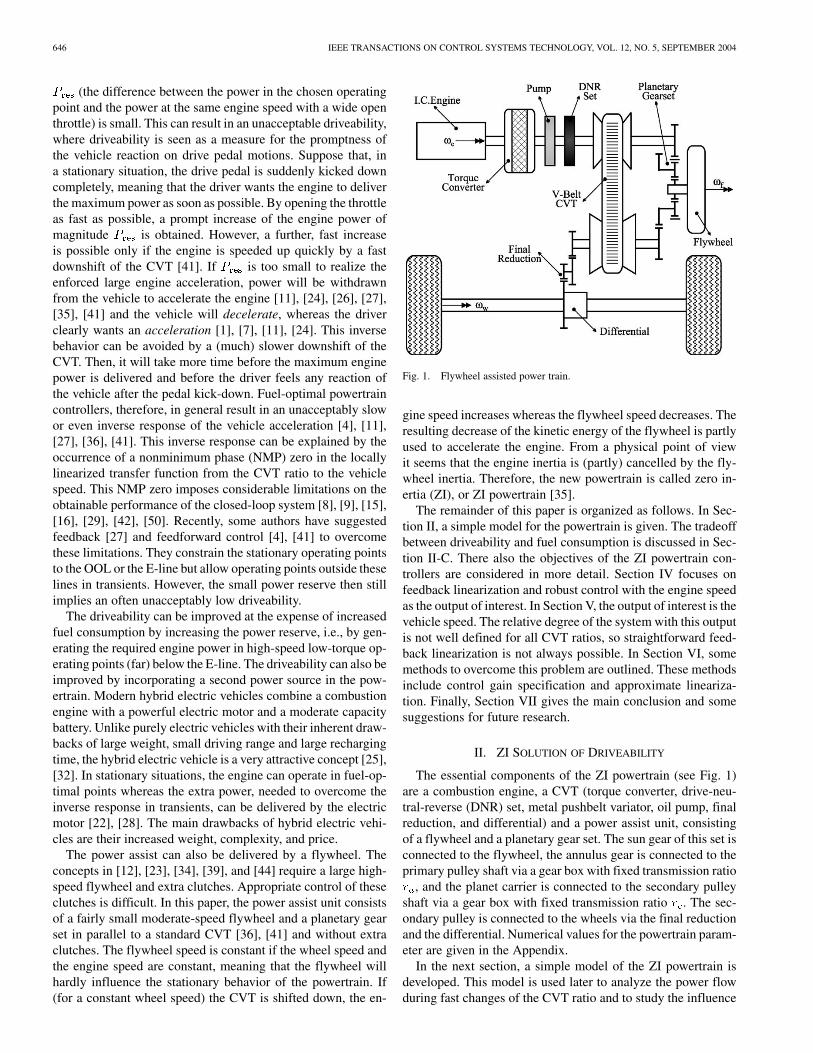
Fig. 1. Flywheel assisted power train.

gine speed increases whereas the flywheel speed decreases. Theresulting decrease of the kinetic energy of the flywheel is partlyused to accelerate the engine. From a physical point of viewit seems that the engine inertia is (partly) cancelled by the fly-wheel inertia. Therefore, the new powertrain is called zero in-ertia (ZI), or ZI powertrain [35].

The remainder of this paper is organized as follows. In Sec-tion II, a simple model for the powertrain is given. The tradeoffbetween driveability and fuel consumption is discussed in Sec-tion II-C. There also the objectives of the ZI powertrain con-trollers are considered in more detail. Section IV focuses onfeedback linearization and robust control with the engine speedas the output of interest. In Section V, the output of interest is thevehicle speed. The relative degree of the system with this outputis not well defined for all CVT ratios, so straightforward feed-back linearization is not always possible. In Section VI, somemethods to overcome this problem are outlined. These methodsinclude control gain specification and approximate lineariza-tion. Finally, Section VII gives the main conclusion and somesuggestions for future research.

II. ZI SOLUTION OF DRIVEABILITY

The essential components of the ZI powertrain (see Fig. 1)are a combustion engine, a CVT (torque converter, drive-neu-tral-reverse (DNR) set, metal pushbelt variator, oil pump, finalreduction, and differential) and a power assist unit, consistingof a flywheel and a planetary gear set. The sun gear of this set isconnected to the flywheel, the annulus gear is connected to theprimary pulley shaft via a gear box with fixed transmission ratio

, and the planet carrier is connected to the secondary pulleyshaft via a gear box with fixed transmission ratio . The sec-ondary pulley is connected to the wheels via the final reductionand the differential. Numerical values for the powertrain param-eter are given in the Appendix.

In the next section, a simple model of the ZI powertrain isdeveloped. This model is used later to analyze the power flowduring fast changes of the CVT ratio and to study the influence

SHEN AND VELDPAUS: ANALYSIS CONTROL OF FLYWHEEL HYBRID VEHICULAR POWERTRAIN 647

Fig. 2. Scheme of the ZI powertrain.

of the flywheel unit on the inverse response. Finally, it will beused for controller design. To evaluate the proposed controllers,the far more realistic model from [37] will be used. However,this simulation model with accurate descriptions of the effi-ciencies of the powertrain components, flexibilities of the driveshafts, etc., will not be described in any detail in this paper.

A. The Controller Design Model

The controller design model is based on simple models forthe engine, the CVT, and the flywheel unit. It is assumed that thevehicle moves along a straight line, that the DNR set is in drivemode, and that the torque converter lock-up clutch is closed. Allflexibilities (including those in the locked convertor and in thedrive shafts) are neglected. A schematic representation of thepowertrain is given in Fig. 2.

The angular speed of the engine is bounded byrad/s and rad/s. In stationary situations, the

engine torque is a function of and the throttle opening ,so2

(1)

The engine torque at speed is upper bounded by the wideopen throttle torque , see Fig. 3. Atspeed , each torque can be realized withan appropriate throttle opening . The torque re-serve in operating point is the difference be-tween the maximum torque at speed and the torque

in that operating point, i.e.,

(2)

In the controller design model, the time delay between a changein the throttle opening and the corresponding change in the en-gine torque is neglected, so (1) is also used in transient situ-ations. Hence, with the engine operating in a stationary point

, a stepwise change of the throttle opening to wide openwill result in a stepwise increase of the torque from the sta-tionary torque to the maximum torqueat speed .

The required fuel mass flow to generate a stationaryengine power is a function of and , so

2The powertrain is equipped with a drive-by-wire system. The applied ac-tuator and controller guarantee that even highly dynamical excursions of thethrottle are realized with negligible errors.

Fig. 3. Engine map.

The engine map of Fig. 3 gives some curves of constant fuelmass flow per unit engine power [brake specific fuel consump-tion (bsfc)]. Also shown is the E-line, i.e., the set of stationaryoperating points in which the delivered power is generated withminimum bsfc.

The torque converter is locked and the DNR set is in drivemode, so the primary pulley speed equals the engine speed

. The secondary pulley speed is related to the angularwheel speed by where is the transmissionratio of the differential plus final reduction. The pulley speedsare also related by , where the transmission ratio

of the applied variator is lower bounded by andupper bounded by the overdrive ratio . Combinationof the given relations results in

(3)

where the so-called CVT ratio , i.e., the overall ratio of thecomplete transmission between the engine and the drivenwheels, is bounded by and . Thisratio is controlled by the clamping forces on the variator pulleys([47]). The CVT is modeled as a first-order system with input

and output , so

(4)

The torques and of the push-belt on the primary andsecondary pulley are related by , where theCVT efficiency is assumed to be constant.

The speed of the sun gear of the planetary set and of theflywheel is a linear function of the annulus speed and thecarrier speed and is given by , wherethe ratio of the annulus radius and the sun gear radius. Besides,

is related to the primary pulley speed bywhereas is related to the secondary pulley speed by

. Combination with yields

(5)

with and . Hence, the flywheelis at rest for any engine speed if the CVT ratio is equal to theso-called geared neutral ratio , i.e.,

(6)

The kinetic energies and the power losses in the flywheel unitare small and are neglected. Therefore, the torque in the shaft


between the annulus gear and the fixed gearing (see Fig. 2)and the torque in the shaft between the planet carrier and thefixed gearing are related to the torque in the shaft betweenthe flywheel and the sun gear by

The equations of motion for the engine side of the powertrain(engine, torque converter, DNR set, primary pulley, gearing ,and annulus wheel), for the wheel side (planet carrier, gearing

, secondary pulley, final reduction, differential, wheels, andvehicle inertia) and for the flywheel part (flywheel and sun gear)are given by

is the moment of inertia of the engine side (reduced to theengine shaft), the moment of inertia of the wheel side (re-duced to the drive shaft), and the moment of inertia of theflywheel part. Furthermore, is the torque in the drive shaftsto the wheels and is given by

Finally, is the external load, consisting of the constant,known rolling resistance torque , the air drag torquewith known constant , and a disturbance torque due toroad slopes, wind gusts, etc.

(7)

Elimination of , , , , , , and and use of(1) results in

(8)

where , the total moment of inertia, is a function of the CVTratio and is given by

(9)

with equivalent moments of inertia and for theengine side and the wheel side

(10)

(11)

With the parameters from the Appendix, it follows thatand

for all , so is positive butcan change sign.

B. Fuel-Optimal Operating Points

Suppose that the disturbance torque is constant and equal to, that the vehicle moves with constant wheel speed

and that the CVT ratio is constant, so , and. Multiplication of this torque balance equation

with and use of (7) and (3) yields the stationary power bal-ance equation

(12)

where is the engine power, required to maintainthe given situation, whereas is the required power at thewheels

Combination of (12) with results in a set oftwo equations for , and . A solution ( , , ) fora given combination ( , ) is called admissible ifthe constraints , , and

are satisfied. Any combination ( , )with at least one admissible solution ( , , ) is called anadmissible vehicle state. In general, there will be more than oneadmissible solution for an admissible vehicle state. One trivialpossibility to arrive at a unique solution is to require that thefuel mass flow in this state is minimal. The problem then is todetermine , , and , such that for the given stationary,admissible vehicle state ( , ) with wheel power

the fuel mass flow is minimizedunder the equality conditions and

and the inequality conditions ,, and . The obtained fuel-op-

timal engine speed is a function of the required engine power, so . With

the optimal throttle opening can be written as a function ofthe engine speed. In summary

(13)

The optimal operating line is the set of all operating points ( ,) for .

C. Behavior After a Pedal Kick Down

Fuel-optimal operating points ( , ) in general combinea high-torque with a low-speed and a smalltorque reserve . As a consequence, the behaviorof a vehicle with an optimally controlled nonhybrid powertrainafter a drive pedal kick-down may be rated unacceptable.Suppose that for the state of the vehicle is stationaryand characterized by ( , ). Let , , , and

be the corresponding fuel-optimalratio, engine speed, throttle opening, and engine torque.Furthermore, suppose that at time the drive pedal is kickeddown completely, meaning that the driver wants the vehicleto accelerate as fast as possible from wheel speed to anew higher speed. To achieve this, the throttle can be openedcompletely as fast as possible, yielding a nearly instantaneousincrease from engine torque to themaximum torque at speed . The equation ofmotion directly after opening the throttle can be written as

(14)

Then only the torque reserve or, formulated in terms ofpower, the power reserve is available to accelerate


the vehicle and the engine. A further fast increase of the poweris possible only if the engine is speeded up quickly by making

large negative, i.e., by a fast downshift of the CVT. However,to avoid vehicle decelerations it follows from (14) that has tosatisfy

(15)

For the conventional vehicle (no extra flywheel, so and) the condition reduces to

Clearly, this condition is not satisfied for large negative valuesof , meaning that the desired fast downshift will result in ahighly undesirable inverse response of the conventional vehiclebecause this vehicle will decelerate initially whereas the driverclearly wants an acceleration.

To solve this problem, the torque reserve can be increased bymoving the stationary engine operating point from the OOL to apoint (far) below this line with higher speed smaller torque andlarger torque reserve but also with a (strongly) increased fuelconsumption. From a fuel economy point of view, it is moreattractive to integrate a torque assist unit in the powertrain. Inthe ZI vehicle, this is materialized by the flywheel unit. For thisvehicle, the condition to avoid the inverse response is given by(15). For a further investigation, (11) for the moment of inertia

is rewritten as

(16)

where the ratio is given by

(17)

It is seen that if , meaning that the engineinertia is compensated by the flywheel if . Therefore,

is called the zero inertia ratio. The engine inertia is morethan compensated if whereas it ispartly compensated if . Fi-nally, if . An ad hoc optimizationof the ZI parameters [6], [37], [48] resulted in a geared neutralratio and a zero inertia ratio with

and with and close to . In all states with mod-erate to large vehicle speeds the fuel-optimal CVT ratiois close to . Starting in such a state, after a pedal kick-down

initially is negative and must be smaller than a posi-tive number to avoid an inverse response. This is not a restrictionsince a large negative value for is wanted to obtain the desiredlarge positive engine acceleration.

For a more physical interpretation of the effect of the fly-wheel, (14) is rewritten as

where the torque is given by

For the conventional vehicle this torque is negative whenever theCVT is shifted down, as will be the case after a pedal kick-down.The so-called torque assist , defined by

represents the influence of the flywheel. This positive torqueassist partly compensates or even overcompensates the negativeconventional torque whenever and .

D. Nonminimum Phase Zero

From a control point of view, the initial inverse response canbe explained by the occurrence of a nonminimum phase (NMP)zero in the linearized transfer function from the transmissioninput to the wheel acceleration . Linearization of system(8) around a stationary ratio , engine speed , and throttleopening , followed by Laplace transformation yields thetransfer functions from perturbations of the throttleopening to perturbations of the wheel acceleration,from perturbations of the CVT input to andfrom perturbations of the disturbance to . The function ofinterest here is . A straightforward calculation results in

(18)

where , the zero of the linearized conventional system,and the pole are given by

with partial derivative , respectively, , of the enginetorque , respectively, the engine power

, with respect to . For all realisticengine operating points, is positive, meaning that theconventional system is nonminimum phase. For the ZI vehicle,this situation only occurs if since only then isnegative. There is no zero if . For , the zero isnegative, i.e., minimum phase. Hence, if no problemsare to be expected for the ZI vehicle, even not if the CVT isshifted down as fast as possible.

III. NONLINEAR CONTROL PHILOSOPHY

The driveline management system (DMS) for the ZI power-train has to determine setpoints for throttle and CVT ratio suchthat the fuel consumption is minimized without compromisingdriveability. The DMS also has to specify the desired state ofthe lockup clutch in the torque convertor and of the drive clutchin the DNR set. Here only the setpoints for the throttle and theCVT ratio are considered. The design of the DMS is based onthe nonlinear model, given by (4) and (8).

Fig. 4 gives a skeleton of the powertrain controller. It con-sists of two layers. The first layer comprises the DMS with su-pervisor, pedal interpreter, and setpoint generator. The pedal in-terpreter translates the drive pedal position into a desired poweror desired torque at the wheels whereas the supervisor speci-fies, amongst others, the desired state of the clutches. The outputof the interpreter and of the supervisor is used by the setpoint


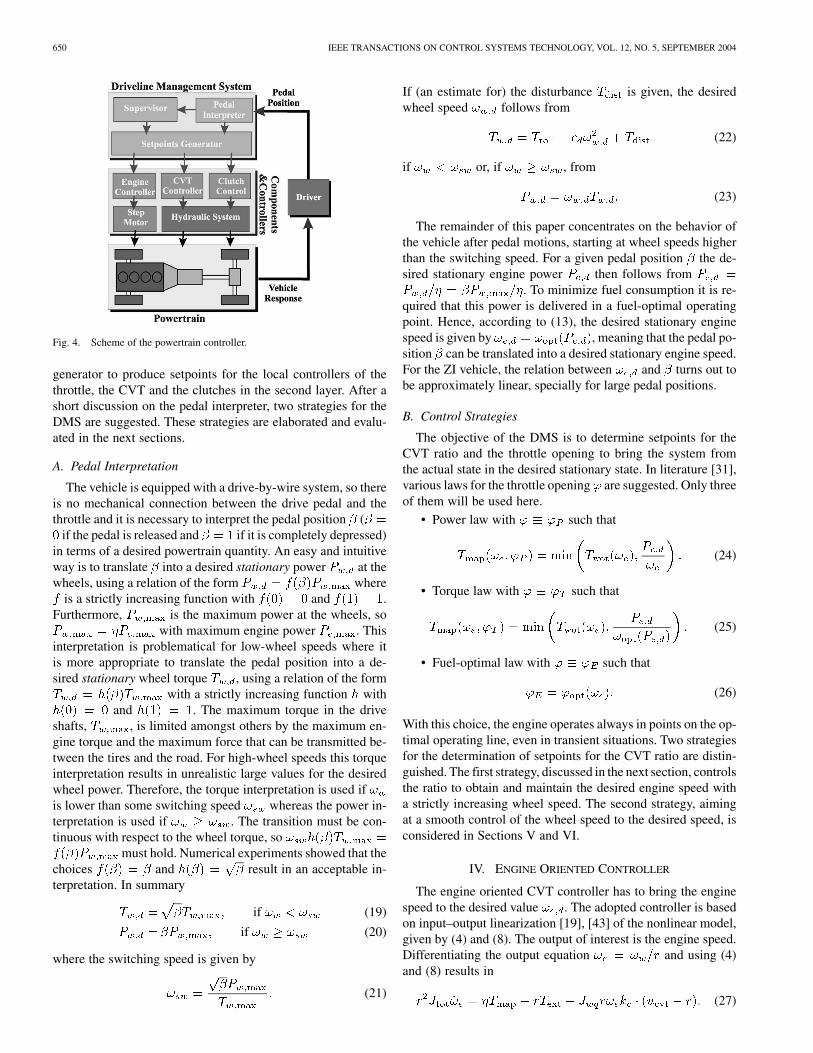
Fig. 4. Scheme of the powertrain controller.

generator to produce setpoints for the local controllers of thethrottle, the CVT and the clutches in the second layer. After ashort discussion on the pedal interpreter, two strategies for theDMS are suggested. These strategies are elaborated and evalu-ated in the next sections.

A. Pedal Interpretation

The vehicle is equipped with a drive-by-wire system, so thereis no mechanical connection between the drive pedal and thethrottle and it is necessary to interpret the pedal position (

if the pedal is released and if it is completely depressed)in terms of a desired powertrain quantity. An easy and intuitiveway is to translate into a desired stationary power at thewheels, using a relation of the form where

is a strictly increasing function with and .Furthermore, is the maximum power at the wheels, so

with maximum engine power . Thisinterpretation is problematical for low-wheel speeds where itis more appropriate to translate the pedal position into a de-sired stationary wheel torque , using a relation of the form

with a strictly increasing function withand . The maximum torque in the drive

shafts, , is limited amongst others by the maximum en-gine torque and the maximum force that can be transmitted be-tween the tires and the road. For high-wheel speeds this torqueinterpretation results in unrealistic large values for the desiredwheel power. Therefore, the torque interpretation is used ifis lower than some switching speed whereas the power in-terpretation is used if . The transition must be con-tinuous with respect to the wheel torque, so

must hold. Numerical experiments showed that thechoices and result in an acceptable in-terpretation. In summary

if (19)

if (20)

where the switching speed is given by

(21)

If (an estimate for) the disturbance is given, the desiredwheel speed follows from

(22)

if or, if , from

(23)

The remainder of this paper concentrates on the behavior ofthe vehicle after pedal motions, starting at wheel speeds higherthan the switching speed. For a given pedal position the de-sired stationary engine power then follows from

. To minimize fuel consumption it is re-quired that this power is delivered in a fuel-optimal operatingpoint. Hence, according to (13), the desired stationary enginespeed is given by , meaning that the pedal po-sition can be translated into a desired stationary engine speed.For the ZI vehicle, the relation between and turns out tobe approximately linear, specially for large pedal positions.

B. Control Strategies

The objective of the DMS is to determine setpoints for theCVT ratio and the throttle opening to bring the system fromthe actual state in the desired stationary state. In literature [31],various laws for the throttle opening are suggested. Only threeof them will be used here.

• Power law with such that

(24)

• Torque law with such that

(25)

• Fuel-optimal law with such that

(26)

With this choice, the engine operates always in points on the op-timal operating line, even in transient situations. Two strategiesfor the determination of setpoints for the CVT ratio are distin-guished. The first strategy, discussed in the next section, controlsthe ratio to obtain and maintain the desired engine speed witha strictly increasing wheel speed. The second strategy, aimingat a smooth control of the wheel speed to the desired speed, isconsidered in Sections V and VI.

IV. ENGINE ORIENTED CONTROLLER

The engine oriented CVT controller has to bring the enginespeed to the desired value . The adopted controller is basedon input–output linearization [19], [43] of the nonlinear model,given by (4) and (8). The output of interest is the engine speed.Differentiating the output equation and using (4)and (8) results in

(27)


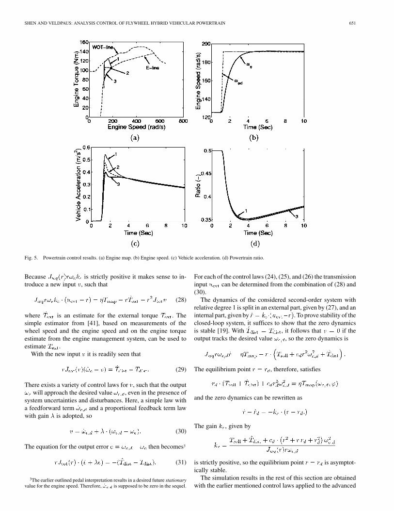
Fig. 5. Powertrain control results. (a) Engine map. (b) Engine speed. (c) Vehicle acceleration. (d) Powertrain ratio.

Because is strictly positive it makes sense to in-troduce a new input , such that

(28)

where is an estimate for the external torque . Thesimple estimator from [41], based on measurements of thewheel speed and the engine speed and on the engine torqueestimate from the engine management system, can be used toestimate .

With the new input it is readily seen that

(29)

There exists a variety of control laws for , such that the outputwill approach the desired value , even in the presence of

system uncertainties and disturbances. Here, a simple law witha feedforward term and a proportional feedback term lawwith gain is adopted, so

(30)

The equation for the output error then becomes3

(31)

3The earlier outlined pedal interpretation results in a desired future stationaryvalue for the engine speed. Therefore, _! is supposed to be zero in the sequel.

For each of the control laws (24), (25), and (26) the transmissioninput can be determined from the combination of (28) and(30).

The dynamics of the considered second-order system withrelative degree 1 is split in an external part, given by (27), and aninternal part, given by . To prove stability of theclosed-loop system, it suffices to show that the zero dynamicsis stable [19]. With , it follows that if theoutput tracks the desired value , so the zero dynamics is

The equilibrium point , therefore, satisfies

and the zero dynamics can be rewritten as

The gain , given by

is strictly positive, so the equilibrium point is asymptot-ically stable.

The simulation results in the rest of this section are obtainedwith the earlier mentioned control laws applied to the advanced


Fig. 6. Results for engine oriented control. (a) Engine speed. (b) Ratio.

simulation model of the ZI vehicle. The disturbance torqueis neglected. For , the pedal position is ,corresponding to an engine speed of 125.5 rad/s and an enginepower of 7.7 kW. At time s the pedal is moved to position

, corresponding to a desired speed of 191.6 rad/s anda desired power of 20.25 kW.

Fig. 5 gives some results for the ZI powertrain. The marks1–3 indicate the results of, respectively, the power, torque, andfuel-optimal throttle control law. Initially the engine operatingpoint is below the E-line because of the limitations on the CVTratio [see Fig. 5(a)]. According to Fig. 5(b), there is a smallsteady-state error in the engine speed. This and the other smalldifferences between the realized and the desired engine speedare caused by the differences between the control design modeland the advanced simulation model, especially with respect tothe modeling of the efficiency of the powertrain components.From Fig. 5(b), it also follows that for s the engine isat its final speed and no power is needed anymore to acceleratethe engine. A very small part of the engine power is used thento accelerate the ZI flywheel whereas the rest is available forthe vehicle. From the same figure it is seen that the differentthrottle control laws result in almost the same course of the en-gine speeds. The reason is that the engine speed, commandedby (29) and (30), does not depend on the applied throttle con-trol law. However, as can be seen from Fig. 5(c), the differentthrottle control laws yield quite different vehicle accelerations.The power law produces the largest accelerations whereas thefuel-optimal law results in the smallest ones. This can also beconcluded from Fig. 5(a), where it is seen that the power lawuses the most of the torque reserve. As a consequence, the CVTratio shift with the power law is a little bit less than with thetorque and the fuel-optimal law [see Fig. 5(d)].

To get an idea of the effect of the extra flywheel, some simu-lations are performed with the fuel-optimal throttle control law,applied to the model for the conventional vehicle. This modeloriginates from the ZI simulation model after substitution of

. The realized engine speeds for the ZI powertrain (solidlines in Fig. 6) are very similar to those of the conventionalpowertrain (dotted lines). Again, this is not surprising since thecourse of the engine speed is governed by the gain in the con-

Fig. 7. Vehicle acceleration.

trol law (30). Two values of are chosen, i.e., s forthe fast case and s for the slow case. From Fig. 6(b),it is seen that the initial down shift of the CVT ratio for the con-ventional powertrain (CCDL in the plots) is marginally fasterthan for the ZI powertrain (ZIPT in the plots). The reason isthat the equivalent moment of inertia of the wheel sideof the ZI powertrain is somewhat larger than the correspondingmoment of the conventional powertrain if .

The results in Fig. 7 clearly demonstrates the initial inverseresponse of the conventional vehicle in the fast case: the acceler-ation is negative for s until s. Furthermore, it isseen that in the slow and also in the fast case, it takes 0.5 s beforethe conventional vehicle accelerates in the desired direction. Forthe ZI powertrain the engine and the vehicle are boosted by thepower from the flywheel unit. For a faster downshift (increasing

), the power flow is larger but can be delivered only during ashorter time interval since the kinetic energy of the flywheel isfairly limited. After reaching the desired engine speed, the con-ventional vehicle accelerates somewhat faster than the ZI ve-hicle because then some engine power is needed to acceleratethe flywheel.


Fig. 8. Results with fuel-optimal law for the throttle. (a) Torque at wheels. (b) Speeds.

From the given results, it may be concluded that the drive-ability (seen as a measure for the vehicle reaction on drive pedalmotions) of the ZI vehicle is much better than that of the con-ventional vehicle. Besides, it turns out that large values of thegain are undesirable for the ZI vehicle to avoid large jerks andfor the conventional vehicle to avoid serious inverse responses.

V. VEHICLE ORIENTED CONTROLLER

In the vehicle oriented CVT controller, a reference forthe wheel speed is determined from the desired wheel power,using the first-order filter

(32)

with the initial condition . The controlleraims to make the actual wheel speed equal to the reference speedin order to realize a smooth transition from the initial speed

to the desired final speed . With the proposed filterfor the reference speed, the actual wheel power will con-verge to the desired value if converges to . In the finalstate the engine has to operate in a fuel-optimal operating point.

Like the engine oriented controller, the vehicle orientedCVT controller is based on input–output linearization, but nowwith the wheel speed as the output of interest. Thus, withas the input, the system (8) is already in the desired form forinput–output linearization. It follows that the relative degree is1 if , i.e., if the CVT ratio differs from the zeroinertia ratio . This will be assumed in the rest of this section.The case where is investigated in Section VI.

If , it makes sense to introduce a new input , suchthat

(33)

and to rewrite the input–output (8) as

(34)

The objective is to find a law for , such that will track thereference . Here a simple law with a feedforward term ,

a proportional feedback term with gain , and a differentialfeedback term with gain is used, so

(35)

The output error then follows from:

(36)

The differential feedback term in (35) is not necessary to guar-antee stability. However, as can be seen from the error equation,this term is helpful in reducing the effect of, e.g., model errorsand external disturbances.

The control law for the transmission input follows from(33) and (35). This law requires an estimate for the externaltorque and, if , also for the wheel acceleration. The ear-lier mentioned estimator from [41] can be used for this purpose.

To evaluate the proposed control law for , simulations areperformed in which the pedal position and the desired power atthe wheels change from and kW for

s to and for s. Thefinal value of the desired power is fairly low to guarantee thatthe CVT ratio will remain larger than for s.

The results in Fig. 8(a) for the driving torque at the wheelsare presented to emphasize that the value of the gains and

in (35) is very important. The solid line, marked “With ,”is determined with the s and whereasboth gains are zero for the line, marked “Without .” The givenvalues for the gains are fairly arbitrary. Fine tuning is desired butis not a subject of this paper. The results for the wheel speed inFig. 8(b) are obtained with the gains s and .This figure shows that goes ahead of . The reason is thatthe adopted tire model in the simulation model requires a certainamount of slip between the tire and the road to produce the forceto propel the vehicle.

The results in Fig. 9 show that the power law (24), markedwith 1, the torque law (25), marked with 2, and the fuel-optimallaw (26), marked with 3, yield practically the same results forthe torque and the power at the wheels. However, the power law


Fig. 9. Results for different throttle control laws. (a) Engine map. (b) Torque at wheels. (c) Power at wheels. (d) Powertrain ratio.

obviously cannot ensure that in the final stationary state the en-gine operates in a point on the optimal operating line. This alsofollows from a closer examination of the zero dynamics. The in-ternal dynamics of the controlled system is described by (4) and(32) after substitution of the control law for . Substitutionof (perfect tracking, ) and of the assumption

in the internal dynamics relations results in the zerodynamics, i.e.,

With (23) for and (7) for , it follows that the equilib-rium point of the zero dynamics system is given byand a solution for of

If the torque law (25) or the fuel-optimal law (26) are used tocontrol the throttle, then the solution for is unique. In bothlaws it is guaranteed that, if the desired power is delivered, itis delivered in an operating point on the optimal operating line.This is not the case for the power law because then any valueof , such that represents an operating point on theisopower line , is a solution. To overcomethis problem, the power law (24) is used only if

where is a small positive number. Otherwise, the powerlaw is replaced by

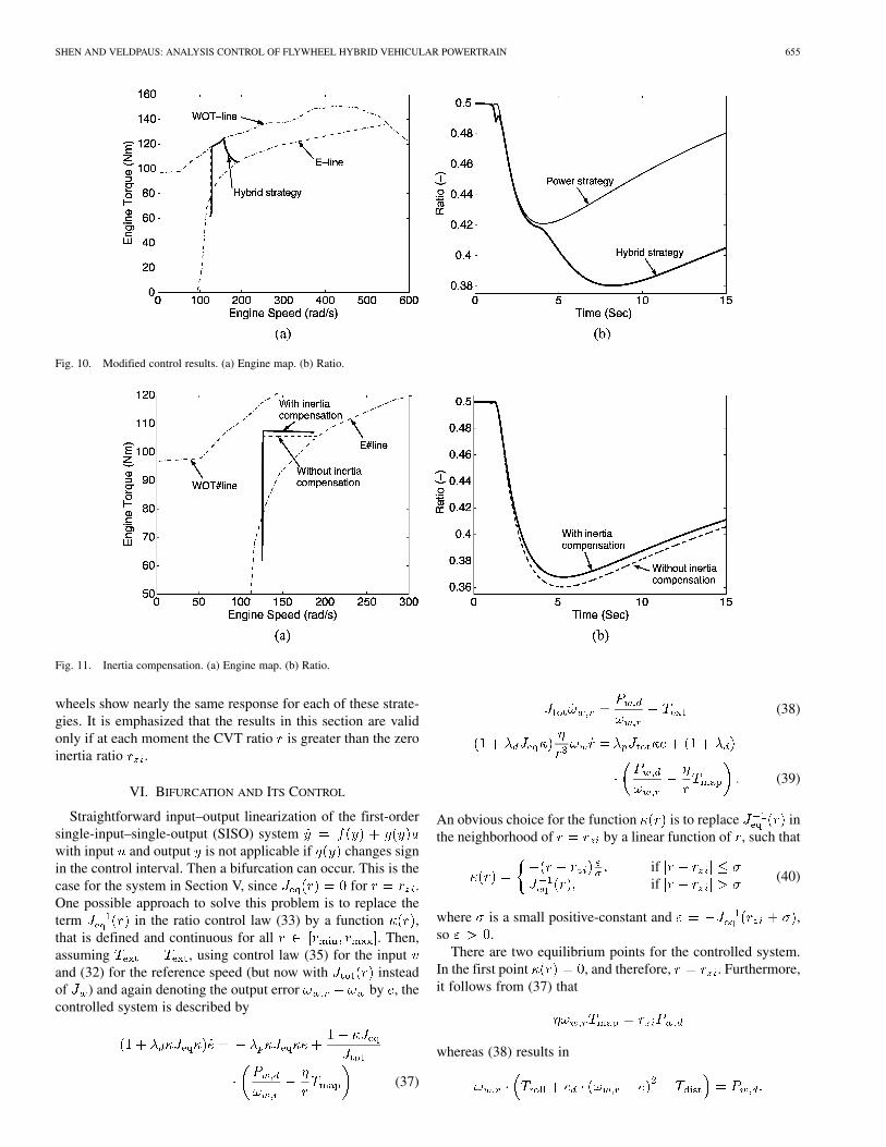
The parameter controls the speed of convergence to theoptimal operating line. The results of the modified strategy inFig. 10 show that the operating point now indeed converges tothis line.

The relation for the desired engine powerneglects the power required to accelerate the engine and

the flywheel. To compensate for this inertia effect, the relationfor is modified into

This modification is meaningful if the power law or the torquelaw are used to control, but not if the fuel-optimal law is used.The results in Fig. 11 are obtained with the torque law. Withthis inertia compensation, the engine delivers a somewhat largertorque whereas the smallest CVT ratio is somewhat larger. Themodification has hardly any influence on the power and torqueat the wheels nor on the wheel speeds.

Several strategies to control the throttle and the CVT are dis-cussed in this section. The behavior of the engine and of thetransmission is quite different for the various strategies but thetorque and the power at the driven wheels and the speed of these


Fig. 10. Modified control results. (a) Engine map. (b) Ratio.

Fig. 11. Inertia compensation. (a) Engine map. (b) Ratio.

wheels show nearly the same response for each of these strate-gies. It is emphasized that the results in this section are validonly if at each moment the CVT ratio is greater than the zeroinertia ratio .

VI. BIFURCATION AND ITS CONTROL

Straightforward input–output linearization of the first-ordersingle-input–single-output (SISO) systemwith input and output is not applicable if changes signin the control interval. Then a bifurcation can occur. This is thecase for the system in Section V, since for .One possible approach to solve this problem is to replace theterm in the ratio control law (33) by a function ,that is defined and continuous for all . Then,assuming , using control law (35) for the inputand (32) for the reference speed (but now with insteadof ) and again denoting the output error by , thecontrolled system is described by

(37)

(38)

(39)

An obvious choice for the function is to replace inthe neighborhood of by a linear function of , such that

ifif (40)

where is a small positive-constant and ,so .

There are two equilibrium points for the controlled system.In the first point , and therefore, . Furthermore,it follows from (37) that

whereas (38) results in


Fig. 12. Bifurcation around r < r . (a) Engine map. (b) Power at wheels. (c) Powertrain ratio.

From these relations, the error and the reference speedin this first equilibrium point can be determined as soon as the(modified) control law for the throttle is specified.

In the second equilibrium point , meaning thatand . Furthermore, it follows that:

and, finally, that

These results, combined with any of the earlier given (modified)laws for the throttle, imply that in the second equilibrium point

and .An analysis of the stability of these equilibrium points learns

that the second equilibrium point is locally asymptotically stablewhereas the first point is unstable.

Fig. 12 gives some results, obtained with the given functionfor a desired stepwise change of the power at the wheels

from 6.4 kW for s to 53.5 kW for s. Two values ofare considered, being (corresponding to )

and (corresponding to ). The gain inthe control law (35) is equal to 0. The torque law (25) is usedto control the throttle. Initially, (because )and , so the CVT will shift down. At s the ratiobecomes equal to and and become equal to

0 and remain equal for some time. Obviously, the CVT cannotshift down to ratios below . The reason is that a bifurcation[38] takes place for . For a further investigation, (39)is linearized around . Substitution of , ofaccording to (40), and of results in

(41)

It turns out that the gain is positive until s, meaningthat and that remains equal to at least until s.In the period form s up to s, the engine speed, theengine power, and the power at the wheels increase but it is notpossible to influence the power flow in the powertrain by theCVT. At s the gain becomes negative, meaning that the

is no longer a stable solution of (41). As a consequence,after s the CVT ratio can increase to the desired level.

The main reason for the observed behavior of the CVT ratiois that the function changes sign for . This problemcan be shunned by choosing a function that is strictly neg-ative or strictly positive for all . This choicestrongly influences the rate of ratio change and the accelera-tion of the driven wheels. Amongst others, it has to be guaran-teed that this acceleration is nonnegative after a kick down ofthe drive pedal. It is noted that may be quite large if is muchlarger than and that should be low if is close to or smaller


Fig. 13. New control gain to overcome bifurcation. (a) Engine speed. (b) Power at wheels. (c) Powertrain ratio.

than . In a first attempt, is chosen as a continuous func-tion, given by

(42)

if , by

(43)

if and by a linear function of if ,i.e.,

(44)

Both and are positive, so is negative for all.

Some results for the closed-loop system, using this withand using the torque law (25) for the throttle are given

in Fig. 13. Now the CVT can shift to lower ratios than be-cause the bifurcation is removed. The stationary error in the en-gine speed in Fig. 6(a) is caused by the differences between thecontrol design model and the simulation model. From Fig. 6(b),it is seen that the response of the power at the wheels now hasa peak at s and oscillates with a large overshoot in theperiod from s to s. Increasing the proportionalgain in the control law (35) results in a decrease of the peak

decreases but also results in more oscillations and a larger over-shoot. To improve the performance, the gain is decreased from

to and the ratio control law (33) is modifiedin two ways. First, the term is replaced not by , butby with according to (42), (43), (44), and de-fined by

where is a positive constant, and .The result of this modification is that the CVT will shift speedis decreased for . Second, to amplifythe influence of the engine torque, the term ismultiplied by a factor . The resulting control law for theCVT ratio then follows from:

Because is positive, is strictly positive and is strictlynegative, it is easy to prove the stability of the equilibrium pointof the closed-loop system. Fig. 14 presents some results for themodified control law with and . Strategy 1means and , strategy 2 refers toand , whereas strategy 3 means and .Comparing these results with those in Fig. 6(b), it can be con-cluded that the improvement is significant. Small values of


Fig. 14. New control gain with better performance. (a) Engine speed. (b) Power at wheels.

reduce the peak in the response of the power at the wheels butalso produce more overshoot. Large values of not only im-prove the peak response but also reduce the overshoot, howeverat the expense of a slower system response. It must be noted thatthe given values for , and are the result of some trial anderror, not of a more or less systematic optimization.

The second method to overcome the problems, caused by thefact that the relative degree is not well defined for ,is based on approximate linearization, e.g., [10] and [14]. It isassumed that . For simplicity, only the torque law(25) is used to control the throttle and it is assumed that at eachmoment with and

. The error between the reference wheel speedand the actual wheel speed is seen as the output of interest.According to [14], a coordinate transformation from ,and to , , and is introduced with the output of interest,so

(45)

Differentiation of this relation with respect to time results in

where the functions and are given by

The relative degree is not well defined in because then. In agreement with [14], the new variable is defined

by

(46)

Differentiation of this relation with respect to time results in

with and given by

where in all relevant situations. Again in agreementwith [14], the control law is chosen as

(47)

With the choice for the third new variable theclosed-loop system is described by

The factor in the control law (47) is introduced here in con-travention of [14] to get more freedom in controlling the shiftspeed of the CVT. Fig. 15 gives some the results, obtained withthis control law with and . Furthermore, fourvalues of , being , , , and , are used.The initial conditions of the system and the desired final stateare the same as in the earlier simulations. The realized powerat the wheels in Fig. 15(b) is quite similar to that in Fig. 14.It turns out that the peak in the response of the power at thewheels can be decreased by increasing the control gain at theexpense of a slower response and an increasing the stationaryerror. Fine tuning of the control parameters , , and tosignificantly improve the performance has not been a topic ofresearch and will be very time consuming. Nevertheless, it maybe concluded that the approximate linearization method is verysuitable to control the ZI powertrain without bifurcation prob-lems.

VII. CONCLUSION

A new concept for a CVT powertrain, called the ZI pow-ertrain, is presented and analyzed. The extra flywheel in thispowertrain can resolve the driveability problems of conventionalpowertrains that are controlled to maximize fuel economy. It is


Fig. 15. Results for approximated linearization. (a) Ratio. (b) Power at wheels.

shown that the inverse behavior of the acceleration of a conven-tional vehicle after a pedal kick down, due to the occurrence ofthe nonminimum phase zero in the linearized transfer functionof the rate of ratio change to this acceleration, is eliminated inthe ZI vehicle. To realize the desired power at the wheels, spec-ified by the pedal interpreter, two types of controllers are de-signed. The first type focuses at the control of the engine speed.Feedback linearization combined with simple techniques fromlinear control theory suffice to obtain the desired behavior ofthis speed. The controllers of the second type concentrate onthe wheel speed. Feedback linearization is more problematic be-cause the relative degree is not well defined then. This resultsin a bifurcation if the transmission ratio becomes equal to theso-called zero inertia ratio. Parameter specification and approx-imate linearization are conducted to overcome the problems, as-sociated with the bifurcation.

The proposed controllers force the engine to work in fuel-op-timal operating points in stationary situations. In transient situa-tions they use the kinetic energy of the extra flywheel to greatlyimprove the behavior of the ZI vehicle compared to an otherwiseidentical vehicle without this flywheel. Although the controllersare designed for the ZI powertrain, they can also be applied toconventional powertrains.

APPENDIX

NOMINAL PARAMETERS

0.0113 Nms .0.224 kgm .135.43 kgm .0.4 kgm .10 s .0.0915.0.4998.0.1227.0.1976.59.93 Nm.0.9578.7.8.0.87.

ACKNOWLEDGMENT

This study is part of EcoDrive, a joint project of Van Doorne’sTransmissie B.V., The Netherlands Organization for AppliedScientific Research, and the Technische Universiteit Eindhoven.

REFERENCES

[1] C. Chan, T. Volz, D. Breitweiser, A. Frank, F. S. Jamzadah, and T.Omitsu, “System Design and Control Considerations of AutomotiveContinuously Variable Transmissions,” in Proc. Int. Congr. Exposition,Detroit, MI, 1984, SAE-Paper 840048.

[2] V. H. L. Cheng and C. A. Desoer, “Limitations on the closed-looptransfer function due to right-half plane transmission zeros of the plant,”IEEE Trans. Automat. Contr., vol. TAC–25, pp. 1218–1220, June 1980.

[3] D. Cho and J. K. Hedrick, “Automotive powertrain modeling for con-trol,” ASME J. Dyn. Sys. Meas. Contr., vol. 111, pp. 568–576, 1989.

[4] M. Deacon, C. J. Brace, N. D. Vaughan, C. R. Burrows, and R. W.Horrocks, “Impact of alternative controller strategies on exhaust emis-sions from an integrated diesel/continuously variable transmission pow-ertrain,” in Proc Inst. Mech. Eng. D, Transp. Eng., vol. 213, 1999, pp.95–107.

[5] R. M. van Druten, B. G. Vroemen, P. C. J. N. Rosielle, F. E. Veldpaus,and W. J. M. Schouten, “Dynamic modeling for dimensioning and con-trol of a flywheel assisted driveline,” in Proc. CVT Conf., Eindhoven,The Netherlands, 1999, pp. 231–237.

[6] R. M. van Druten, “Transmission design of the zero inertia powertrain,”Ph.D. dissertation, Tech. Univ. Eindhoven, Eindhoven, The Netherlands,2001.

[7] F. A. Frank and P. B. Pires, “A high torque, high efficiency cvt for electricvehicles,” in Elect. Veh. Design Development, 1991, SAE-Paper 910251.

[8] J. S. Freudenberg and D. P. Looze, “Right half poles and zeros and de-sign tradeoffs in feedback systems,” IEEE Trans. Automat. Contr., vol.TAC–30, pp. 555–565, June 1985.

[9] J. S. Freudenberg, R. H. Middleton, and A. Stefanopoulou, “A surveyof inherent design limitation,” in American Contr. Conf. Workshop Tu-torial, vol. 5, Chicago, IL, 2000, pp. 2987–3001.

[10] R. Ghanadan and G. L. Blankenship, “Adaptive control of nonlinear sys-tems via approximate linearization,” IEEE Trans. Automat. Contr., vol.41, pp. 618–625, Apr. 1996.

[11] L. Guzzella and A. M. Schmid, “Feeback linearization of spark-ignitionengines with continuously variable transmission,” IEEE Trans. Contr.Syst. Technol., vol. 3, pp. 54–60, Jan. 1995.

[12] L. Guzzella, C. Wittmer, and M. Ender, “Optimal operation of drivetrains with SI-engines and flywheels,” in IFAC 13th World Congr., SanFrancisco, CA, 1996, pp. 237–242.

[13] I.-J. Ha, A. K. Tugcu, and N. M. Boustany, “Feeback linearization con-trol of vehicle longitudinal acceleration,” IEEE Trans. Automat. Contr.,vol. 34, pp. 689–698, July 1989.

[14] J. Hauser, S. Sastry, and P. Kokotovic, “Nonlinear control via approx-imate input–output linearization: the ball and beam example,” IEEETrans. Automat. Contr., vol. 37, pp. 392–398, Mar. 1992.


[15] I. Horowitz, “Design of feedback systems with nonminimum phase un-stable plants,” Int. J. Syst. Sci., vol. 10, pp. 1025–1040, 1979.

[16] I. Horowitz and Y. Liau, “Limitations of with nonminimum-phase feed-back systems,” Int. J. Control, vol. 40, no. 5, pp. 1003–1013, 1984.

[17] D. Hrovat and W. F. Powers, “Computer control systems for automotivepower trains,” IEEE Control Syst. Mag., vol. 8, pp. 3–10, Apr. 1988.

[18] D. V. Huwang, “Fundamental Parameters of Vehicle Fuel Economy andAcceleration,” 1969 SAE Trans., 1969.

[19] A. Isidori, Nonliear Control Systems. New York: Springer-Verlag,1995.

[20] U. Kienche, “A view of automotive control systems,” IEEE Control Syst.Mag., vol. 8, pp. 11–19, Apr. 1988.

[21] T. Kim and H. Kim, “Performance of an integrated engine-CVT control,considering powertrain loss and CVT response lag,” in Proc. ImechEIntegrated Powertrains Control, Bath, U.K., 2000, pp. 31–45.

[22] A. Kleimaier and D. Schroeder, “Optimized design and control of a hy-brid drivetrain with a CVT,” in Proc. 1st IFAC Conf. Mechatronic Sys-tems, Darmstadt, Germany, 2000, pp. 197–202.

[23] D. B. Kok, “Design optimization of a flywheel hybrid vehicle,” Ph.D.dissertation, Tech. Univ. Eindhoven, Eindhoven, The Netherlands, 1999.

[24] I. Kolmanovsky, J. Sun, and L. Wang, “Coordinated control of lean burngasoline engines with continuously variable transmissions,” in Proc.American Control Conf., vol. 4, San Diego, CA, 1999, pp. 2673–2677.

[25] H. D. Lee and S. K. Sul, “Fuzzy-logic-based torque control strategy forparallel-type hybrid electric vehicle,” IEEE Trans. Ind. Electron., vol.45, pp. 625–632, Aug. 1998.

[26] S. Liu and B. Paden, “A survey of today’s CVT controls,” in Proc. 36thCDC Conf., San Diego, CA, 1997, pp. 4738–4743.

[27] S. Liu, A. G. Stefanopoulou, and B. E. Paden, “Effects of control struc-ture on performance for an automotive powertrain with a continuouslyvariable transmission,” presented at the AVEC2000 Conf., Ann Arbor,MI, 2000, [CD-ROM] Paper nr 054.

[28] T. Mayer and D. Schroeder, “Robust Control of a Parallel Hybrid Driv-etrain With a CVT,” SAE, Tech. Paper 960233, 1996.

[29] R. H. Middleton, “Trade-offs in linear control system design,” Auto-matica, vol. 27, no. 2, pp. 281–292, 1991.

[30] A. Numazawa et al., “Automatic transmission optimization for betterfuel economy,” in Proc. FISITA Conf., 1978.

[31] R. A. J. Pfiffner, “Optimal operation of CVT-based powertrains,” Ph.D.dissertation, Swiss Federal Inst. Technol., Zürich, Switzerland, 2001.

[32] B. K. Powell, K. E. Bailey, and S. R. Cikanek, “Dynamic modeling andcontrol of hybrid electric vehicle powertrain systems,” IEEE ControlSyst. Mag., vol. 18, no. 5, pp. 17–23, 1998.

[33] S. Sakaguchi, E. Kimura, and K. Yamamoto, “Development of an En-gine-CVT Integrated Control System,” in Proc. Int. Congr. Exposition,Detroit, MI, Mar. 1999, SAE-Paper 1999-01-0754.

[34] A. Schmid, P. Dietrich, S. Ginsburg, and H. P. Geering, “Controlling aCVT-Equipped Hybrid Car,” SAE, Tech. Paper 950 492, 1995.

[35] A. F. A. Serrarens and F. E. Veldpaus, “Dynamic modeling for dimen-sioning and control of a flywheel assisted driveline,” in Proc. EAECConf., Barcelona, Spain, 1999, pp. 261–268.

[36] , “New concepts for power transients in flywheel assisted drivelineswith a CVT,” presented at the FISITA World Automotive Conf., Seoul,Korea, 2000, [CD-ROM] Paper nr F2000A129.

[37] A. F. A. Serrarens, “Coordinated control of the zero inertia powertrain,”Ph.D. dissertation, Tech. Univ. Eindhoven, Eindhoven, The Netherlands,2001.

[38] R. Seydel, Practical Bifurcation and Stability Analysis: From Equilib-rium to Chaos. New York: Springer-Verlag, 1994.

[39] E. Shafai, A. Schmid, and H. P. Geering, “Torque Pedel for a Car Witha Continuously Variable Transmission,” Transmission Drivelines, ser.SAE Special Publication, vol. 1032, 1994.

[40] S. Shen, H. Tanaka, and Y. Sato, “Simulating a CVT vehicle economywith the method of an engine universal performance map,” in Proc. 15thInt. Combustion Engine Symp., Seoul, Korea, 1999.

[41] S. Shen, A. F. A. Serrarens, M. Steinbuch, and F. E. Veldpaus, “Con-trol of a hybrid driveline for fuel economy and driveability,” in Proc.AVEC2000 Conf., Ann Arbor, MI, pp. 469–475.

[42] M. Sidi, “Gain-bandwidth limitations of feedback systems with nonmin-imum phase plants,” Int. J. Control, vol. 67, no. 5, pp. 731–743, 1997.

[43] J.-J. Slotine and W. Li, Applied Nonlinear Control. Englewood Cliffs,NJ: Prentice-Hall, 1991.

[44] E. Spijker, “Steering and control of a CVT based hybrid transmission fora passenger car,” Ph.D. dissertation, Tech. Univ. Eindhoven, Eindhoven,The Netherlands, 1994.

[45] S. Takahashi, “Fundamental study of low fuel consumption controlscheme based on combination of direct fuel injection engine andcontinuously variable transmission,” in Proc. 37th CDC Conf., Tampa,FL, 1998, pp. 1522–1529.

[46] T. Takiyama and S. Morita, “Engine-CVT consolidated control usingLQI control theory,” JSAE Rev., vol. 20, pp. 251–258, 1999.

[47] B. G. Vroemen and F. E. Veldpaus, “Control of a CVT in a flywheelassisted driveline,” presented at the Proc. FISITA World AutomotiveConf., Seoul, Korea, 2000, [CR-ROM] Paper nr F2000A133.

[48] , “Component control for the zero inertia powertrain,” Ph.D. dis-sertation, Tech. Univ. Eindhoven, Eindhoven, The Netherlands, 2001.

[49] M. Yasuoka, M. Uchida, S. Katakura, and T. Yoshino, “An IntegratedControl Algorithm for an SI Engine and a CVT,” in Proc. Transmis-sion Driveline Systems Symp., 1999, SAE Tech. Paper 1999-01-0752,pp. 155–160.

[50] Z. Zhang and J. S. Freudenberg, “Loop transfer recovery for nonmin-imum phase plants,” IEEE Trans. Automat. Contr., vol. 35, pp. 547–553,May 1990.

Shuiwen Shen was born on October 17, 1967. He re-ceived the B.S., M.S., and Ph.D. degrees in mechan-ical engineering from the Jilin University of Tech-nology, Jilin, China, in 1990, 1992, and 1996, respec-tively.

He worked at the Shanghai Jiaotong University,China as a Post-Doctororal Fellow from 1996 to1998, as a Guest Lecturer at Yokohama NationalUniversity, Japan, from 1998 to 1999, and as aResearch Fellow at the Eindhoven University ofTechnology, The Netherlands, from 1999 to 2001.

He currently works as a Research Fellow at the University of Leeds, Leeds,U.K. His research interests include modeling and control of advanced andhybrid vehicular power trains, steering control, vehicular handling and, moregeneral, robust and nonlinear control and their applications to complexmechanical systems.

Frans E. Veldpaus was born on July 1, 1942. Hereceived the M.S. and Ph.D. degrees from the Tech-nische Universiteit Eindhoven (TU/e), Eindhoven,The Netherlands, in 1966 and 1973, respectively.

Since 1996, he has worked in the Department ofMechanical Engineering, TU/e, first in the area ofstructural dynamics and solid mechanics and then inthe field of control of mechanical systems. His mainresearch activities concern modeling and control ofautomotive systems, i.e., of active wheel suspensionsand power trains in general and of automotive com-

ponents like clutches and continuously variable transmissions in particular.

leica m844 f40 - leica microsystems

Documents