lectures part 20
DESCRIPTION
Lectures Part 20TRANSCRIPT
Computational Biology, Part 20
Neuronal Modeling
Robert F. MurphyRobert F. MurphyCopyright Copyright 1996, 1999- 1996, 1999-
2006.2006.All rights reserved.All rights reserved.

Basic Neurophysiology An imbalance of charge across a An imbalance of charge across a membrane is called a membrane is called a membrane membrane potentialpotential
The major contribution to membrane The major contribution to membrane potential in animal cells comes from potential in animal cells comes from imbalances in small ions (e.g., Na, imbalances in small ions (e.g., Na, K)K)
The maintenance of this imbalance is The maintenance of this imbalance is an an activeactive process carried out by ion process carried out by ion pumpspumps

Basic Neurophysiology The cytoplasm of most cells The cytoplasm of most cells (including neurons) has an excess (including neurons) has an excess of negative ions over positive ions of negative ions over positive ions (due to active pumping of sodium (due to active pumping of sodium ions out of the cell)ions out of the cell)
By convention this is referred to By convention this is referred to as a as a negative membrane potential negative membrane potential (inside minus outside)(inside minus outside)
Typical Typical resting potential resting potential is -50 mVis -50 mV
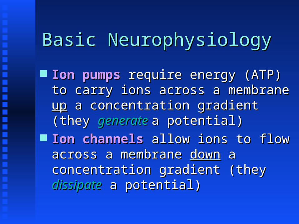
Basic Neurophysiology Ion pumps Ion pumps require energy (ATP) require energy (ATP) to carry ions across a membrane to carry ions across a membrane upup a concentration gradient a concentration gradient (they (they generate generate a potential)a potential)
Ion channels Ion channels allow ions to flow allow ions to flow across a membrane across a membrane downdown a a concentration gradient (they concentration gradient (they dissipatedissipate a potential) a potential)

Basic Neurophysiology A cell is said to be electrically A cell is said to be electrically polarizedpolarized when it has a non-zero when it has a non-zero membrane potentialmembrane potential
A dissipation (partial or total) A dissipation (partial or total) of the membrane potential is of the membrane potential is referred to as a referred to as a depolarizationdepolarization, , while restoration of the resting while restoration of the resting potential is termed potential is termed repolarizationrepolarization
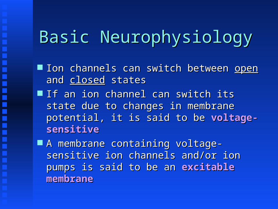
Basic Neurophysiology Ion channels can switch between Ion channels can switch between openopen and and closedclosed states states
If an ion channel can switch its If an ion channel can switch its state due to changes in membrane state due to changes in membrane potential, it is said to be potential, it is said to be voltage-voltage-sensitivesensitive
A membrane containing voltage-A membrane containing voltage-sensitive ion channels and/or ion sensitive ion channels and/or ion pumps is said to be an pumps is said to be an excitable excitable membranemembrane

Basic Neuro-physiology
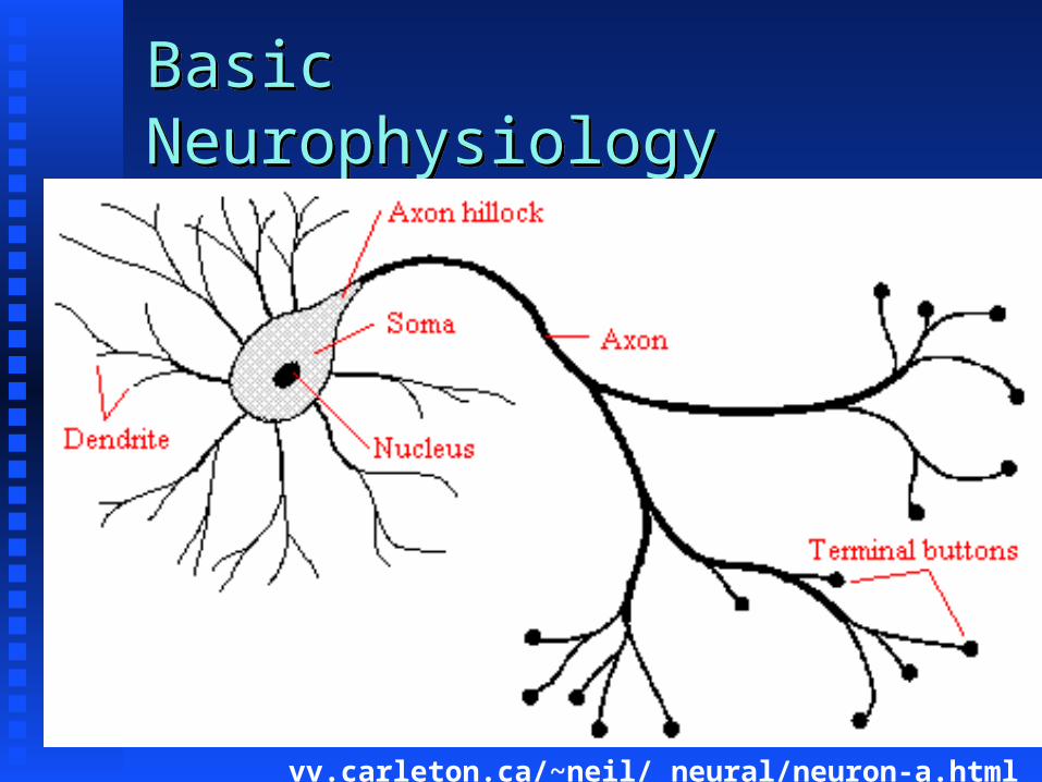
An idealized An idealized neuronneuron consists of consists of somasoma or or cell bodycell body
contains nucleus and performs metabolic contains nucleus and performs metabolic functionsfunctions
dendritesdendrites receive signals from other neurons receive signals from other neurons through through synapsessynapses
axonaxon propagates signal away from somapropagates signal away from soma
terminal branchesterminal branches form form synapsessynapses with other neurons with other neurons
Basic Neurophysiology
vv.carleton.ca/~neil/ neural/neuron-a.html
Basic Neuro-physiology
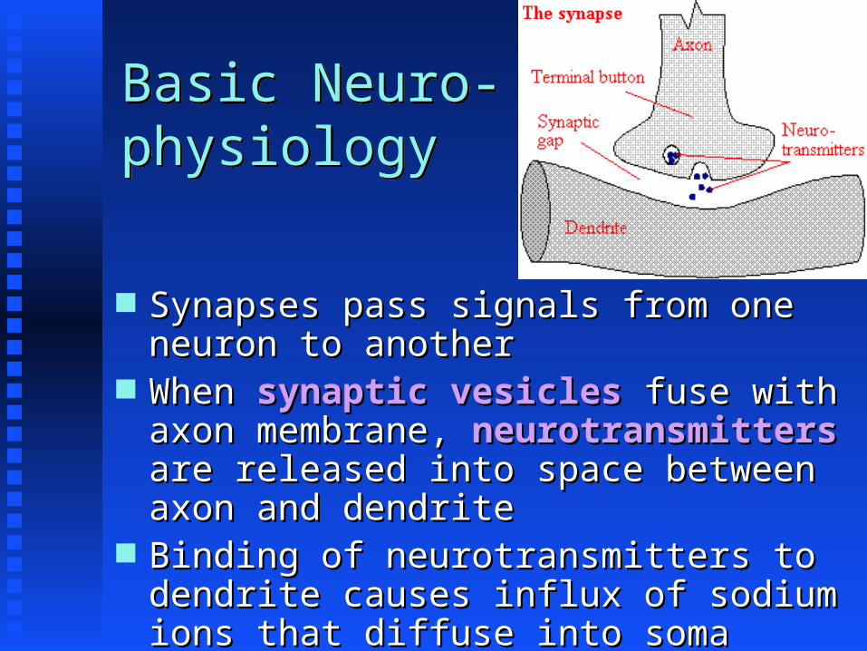
Synapses pass signals from one Synapses pass signals from one neuron to anotherneuron to another
When When synaptic vesiclessynaptic vesicles fuse with fuse with axon membrane, axon membrane, neurotransmittersneurotransmitters are released into space between are released into space between axon and dendriteaxon and dendrite
Binding of neurotransmitters to Binding of neurotransmitters to dendrite causes influx of sodium dendrite causes influx of sodium ions that diffuse into soma ions that diffuse into soma

Basic Neurophysiology The junction between the soma and The junction between the soma and the axon is called the the axon is called the axonaxon hillockhillock
The soma sums (“integrates”) The soma sums (“integrates”) currents (“inputs”) from the currents (“inputs”) from the dendritesdendrites
When the received currents result in When the received currents result in a sufficient change in the membrane a sufficient change in the membrane potential, a rapid depolarization is potential, a rapid depolarization is initiated in the axon hillockinitiated in the axon hillock

Basic Neurophysiology The depolarization is caused by The depolarization is caused by opening of voltage-sensitive opening of voltage-sensitive sodium channels that allow sodium sodium channels that allow sodium ions to flow into the cellions to flow into the cell
The sodium channels only open in The sodium channels only open in response to a partial response to a partial depolarization, such that a depolarization, such that a threshold voltage threshold voltage is exceededis exceeded
Basic Neurophysiology As sodium floods in, the membrane As sodium floods in, the membrane potential reverses, such that the potential reverses, such that the interior is now positive relative to interior is now positive relative to the outsidethe outside
This positive potential causes This positive potential causes voltage-sensitive potassium channels voltage-sensitive potassium channels to open, allowing Kto open, allowing K++ ions to flow out ions to flow out
The potential overshoots (becomes The potential overshoots (becomes more negative than) the resting more negative than) the resting potentialpotential

Basic Neurophysiology The fall in potential triggers The fall in potential triggers the sodium channels to close, the sodium channels to close, setting the stage for restoration setting the stage for restoration of the resting potential by of the resting potential by sodium pumpssodium pumps
This sequential depolarization, This sequential depolarization, polarity reversal, potential polarity reversal, potential overshoot and repolarization is overshoot and repolarization is called an called an action potentialaction potential
Action Potential
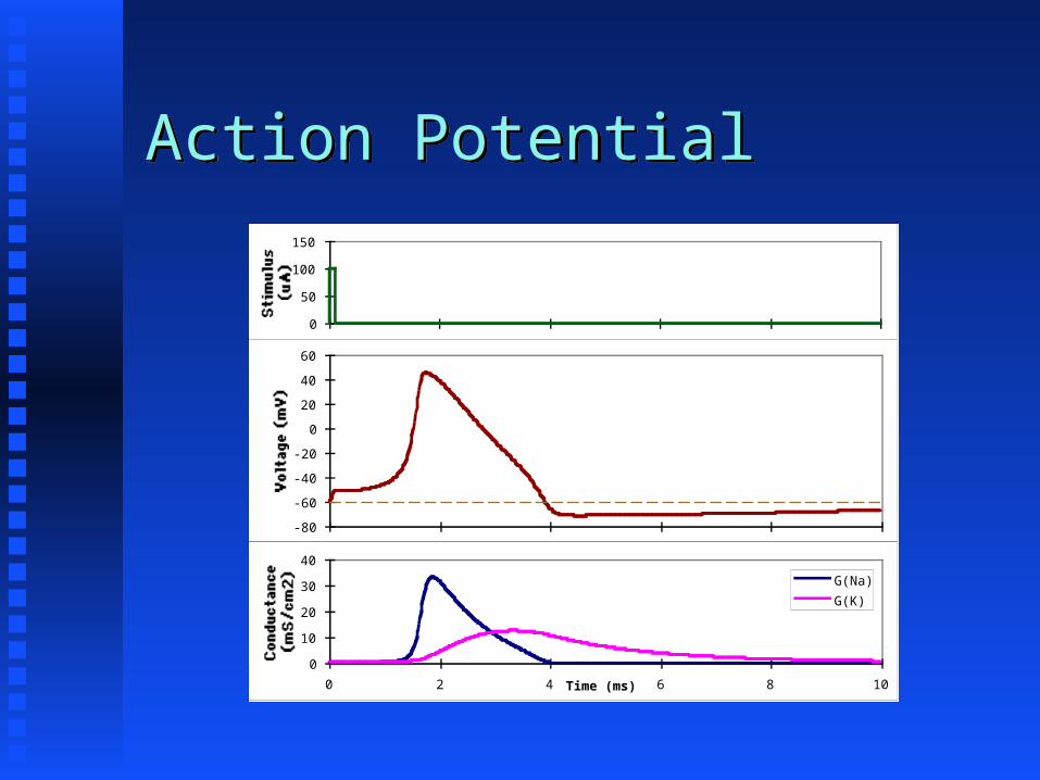
-80-60-40-20
0204060
Voltage (mV)
010203040
0 2 4 6 8 10Time (ms)
Conductance (mS/cm2)
G(Na)G(K)
050
100150
Stimulus (uA)

Basic Neurophysiology The depolarization in the axon The depolarization in the axon hillock causes a depolarization in hillock causes a depolarization in the region of the axon immediately the region of the axon immediately adjacent to the hillockadjacent to the hillock
Depolarization (and repolarization) Depolarization (and repolarization) proceeds down the axon until it proceeds down the axon until it reaches the terminal branchesreaches the terminal branches
The depolarization causes synaptic The depolarization causes synaptic vesicles to fuse with the membrane, vesicles to fuse with the membrane, releasing neurotransmitters to releasing neurotransmitters to stimulate neurons with which they stimulate neurons with which they form synapsesform synapses

Basic Neurophysiology These sequential These sequential depolarizations form a depolarizations form a traveling wavetraveling wave passing down the passing down the axonaxon
Note that while a signal is Note that while a signal is passed down the axon, it is passed down the axon, it is notnot comparable to an electrical comparable to an electrical signal traveling down a cablesignal traveling down a cable

Basic Neurophysiology Current flows in an electrical Current flows in an electrical cablecable are in the direction that the signal are in the direction that the signal is propagatingis propagating
consist of electronsconsist of electrons Current flows in a neuronCurrent flows in a neuron
are transverse to the signal are transverse to the signal propagationpropagation
consist of positively-charged ionsconsist of positively-charged ions

The Hodgkin-Huxley Model Based on electrophysiological Based on electrophysiological measurements of giant squid measurements of giant squid axonaxon
Empirical model that predicts Empirical model that predicts experimental data with very experimental data with very high degree of accuracyhigh degree of accuracy
Provides insight into Provides insight into mechanism of action potentialmechanism of action potential

The Hodgkin-Huxley Model DefineDefine
v(t) v(t) voltage across the membrane at time voltage across the membrane at time tt
q(t) q(t) net charge inside the neuron at net charge inside the neuron at tt I(t) I(t) current of positive ions into neuron current of positive ions into neuron at at tt
g(v) g(v) conductance of membrane at voltage conductance of membrane at voltage vv CC capacitance of the membranecapacitance of the membrane Subscripts Na, K and L used to denote Subscripts Na, K and L used to denote specific currents or conductances specific currents or conductances (L=“other”)(L=“other”)
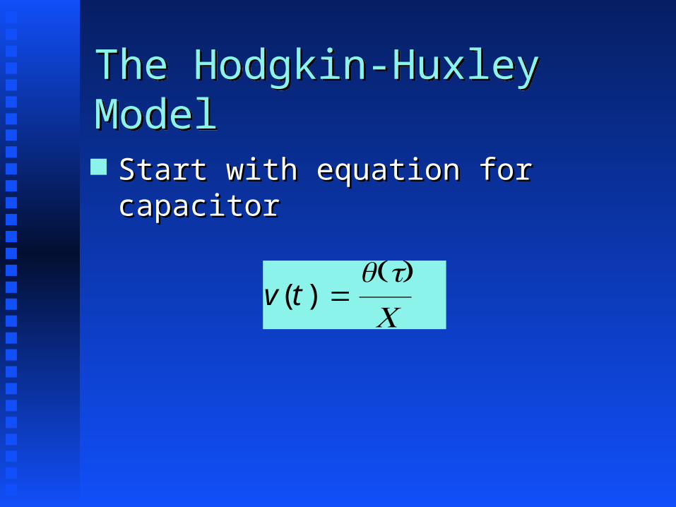
The Hodgkin-Huxley Model Start with equation for Start with equation for capacitorcapacitor
v(t ) =q(t)
C

The Hodgkin-Huxley Model Consider each ion separately Consider each ion separately and sum currents to get rate and sum currents to get rate of change in charge and hence of change in charge and hence voltagevoltage dq
dt=I Na + I K + I L
I Na =gNa(v−vNa)I K =gK (v−vK )I L =gL (v−vL )
dvdt
=−1
CgNa(v)(v−vNa) + gK (v)(v−vK ) + gL (v−vL )[ ]

The Hodgkin-Huxley Model Central concept of model: Central concept of model: Define three state variables Define three state variables that represent (or “control”) that represent (or “control”) the opening and closing of the opening and closing of ion channelsion channels mm controls Na channel opening controls Na channel opening hh controls Na channel closing controls Na channel closing nn controls K channel opening controls K channel opening
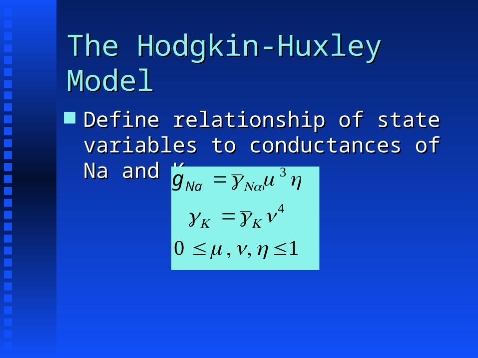
The Hodgkin-Huxley Model Define relationship of state Define relationship of state variables to conductances of variables to conductances of Na and KNa and Kg Na =gNam 3 h
gK =gK n 4
0 ≤m , n, h ≤1
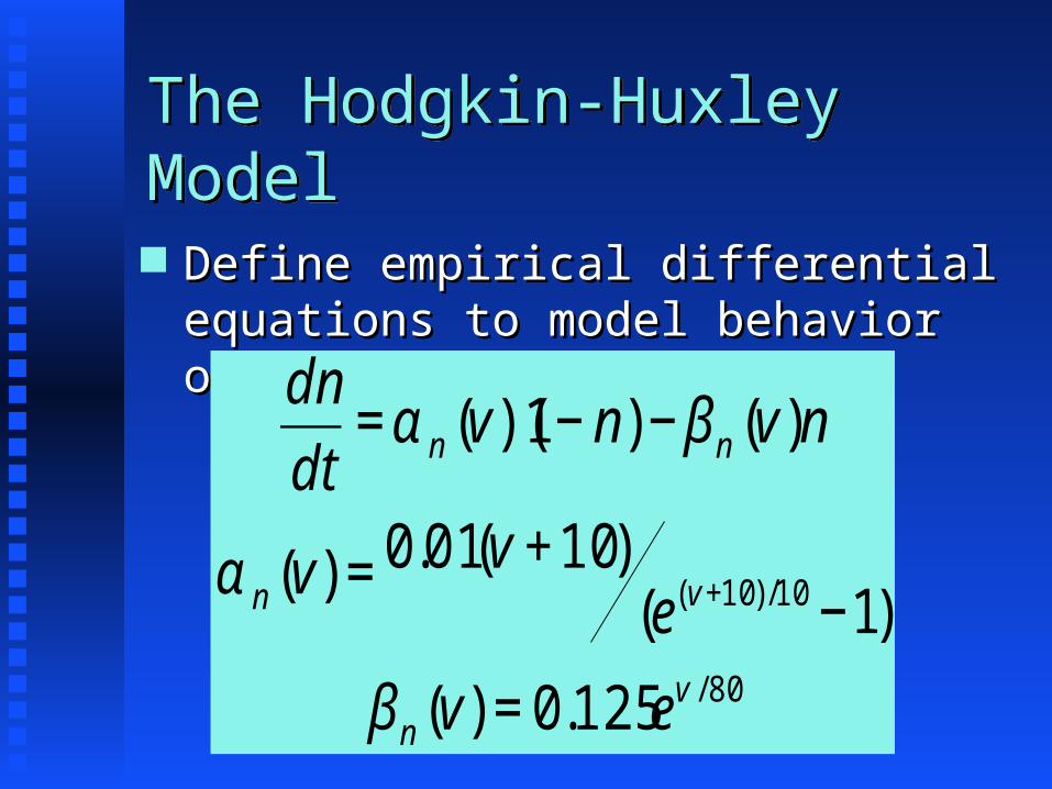
The Hodgkin-Huxley Model Define empirical differential Define empirical differential equations to model behavior equations to model behavior of each gateof each gate
€
dndt=α n (v)(1− n) −β n (v)n
α n (v) =0.01(v +10)
(e(v+10)/10 −1)β n (v) = 0.125e
v / 80
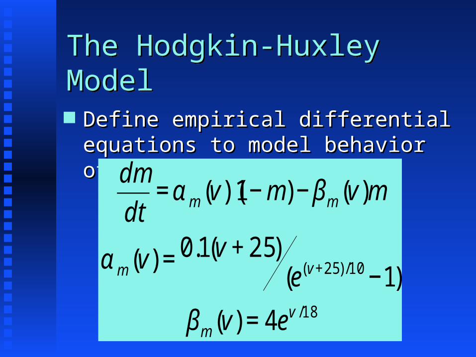
The Hodgkin-Huxley Model Define empirical differential Define empirical differential equations to model behavior equations to model behavior of each gateof each gate
€
dmdt=α m (v)(1−m) −βm (v)m
α m (v) =0.1(v + 25)
(e(v+25)/10 −1)βm (v) = 4e
v /18

The Hodgkin-Huxley Model Define empirical differential Define empirical differential equations to model behavior equations to model behavior of each gateof each gate
€
dhdt=α h (v)(1− h) −β h (v)h
α h (v) = 0.07ev / 20
β h (v) = 1(e(v+30)/10 +1)
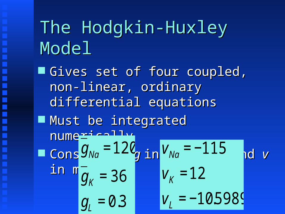
The Hodgkin-Huxley Model Gives set of four coupled, Gives set of four coupled, non-linear, ordinary non-linear, ordinary differential equationsdifferential equations
Must be integrated Must be integrated numericallynumerically
Constants (Constants (g g in mmho/cmin mmho/cm22 and and vv in mV) in mV)
€
gNa =120
gK = 36gL = 0.3
€
vNa = −115vK =12vL = −10.5989

Hodgkin-Huxley Gates
-80-60-40-20
0204060
Voltage (mV)
050
100150
Stimulus (uA)
0.00.20.40.60.81.0
0 2 4 6 8 10Time (ms)
Gate param value
m gate (Na)h gate (Na)n gate (K)
Interactive demonstration (Integration of Hodgkin-(Integration of Hodgkin-Huxley equations using Maple)Huxley equations using Maple)

Interactive demonstration
> Ena:=55: Ek:=-82: El:= -59: gkbar:=24.34: gnabar:=70.7: > Ena:=55: Ek:=-82: El:= -59: gkbar:=24.34: gnabar:=70.7: > gl:=0.3: vrest:=-69: cm:=0.001:> gl:=0.3: vrest:=-69: cm:=0.001:> alphan:=v-> 0.01*(10-(v-vrest))/(exp(0.1*(10-(v-vrest)))-> alphan:=v-> 0.01*(10-(v-vrest))/(exp(0.1*(10-(v-vrest)))-
1):1):> betan:=v-> 0.125*exp(-(v-vrest)/80):> betan:=v-> 0.125*exp(-(v-vrest)/80):> alpham:=v-> 0.1*(25-(v-vrest))/(exp(0.1*(25-(v-vrest)))-1):> alpham:=v-> 0.1*(25-(v-vrest))/(exp(0.1*(25-(v-vrest)))-1):> betam:=v-> 4*exp(-(v-vrest)/18):> betam:=v-> 4*exp(-(v-vrest)/18):> alphah:=v->0.07*exp(-0.05*(v-vrest)):> alphah:=v->0.07*exp(-0.05*(v-vrest)):> betah:=v->1/(exp(0.1*(30-(v-vrest)))+1):> betah:=v->1/(exp(0.1*(30-(v-vrest)))+1):> pulse:=t->-20*(Heaviside(t-.001)-Heaviside(t-.002)):> pulse:=t->-20*(Heaviside(t-.001)-Heaviside(t-.002)):> rhsV:=(t,V,n,m,h)->-(gnabar*m^3*h*(V-Ena) +> rhsV:=(t,V,n,m,h)->-(gnabar*m^3*h*(V-Ena) +> > gkbar*n^4*(V-Ek) + gl*(V-gkbar*n^4*(V-Ek) + gl*(V-
El)+ pulse(t))/cm:El)+ pulse(t))/cm:> rhsn:=(t,V,n,m,h)-> 1000*(alphan(V)*(1-n) - betan(V)*n):> rhsn:=(t,V,n,m,h)-> 1000*(alphan(V)*(1-n) - betan(V)*n):> rhsm:=(t,V,n,m,h)-> 1000*(alpham(V)*(1-m) - betam(V)*m):> rhsm:=(t,V,n,m,h)-> 1000*(alpham(V)*(1-m) - betam(V)*m):> rhsh:=(t,V,n,m,h)-> 1000*(alphah(V)*(1-h) - betah(V)*h):> rhsh:=(t,V,n,m,h)-> 1000*(alphah(V)*(1-h) - betah(V)*h):

Interactive demonstration
> inits:=V(0)=vrest,n(0)=0.315,m(0)=0.042, h(0)=0.608;> inits:=V(0)=vrest,n(0)=0.315,m(0)=0.042, h(0)=0.608;> sol:=dsolve({diff(V(t),t)=rhsV(t,V(t),n(t),m(t),h(t)),> sol:=dsolve({diff(V(t),t)=rhsV(t,V(t),n(t),m(t),h(t)), diff(n(t),t)=rhsn(t,V(t),n(t),m(t),h(t)),diff(n(t),t)=rhsn(t,V(t),n(t),m(t),h(t)), diff(m(t),t)=rhsm(t,V(t),n(t),m(t),h(t)),diff(m(t),t)=rhsm(t,V(t),n(t),m(t),h(t)), diff(h(t),t)=rhsh(t,V(t),n(t),m(t),h(t)),inits},diff(h(t),t)=rhsh(t,V(t),n(t),m(t),h(t)),inits}, {V(t),n(t),m(t),h(t)},type=numeric, {V(t),n(t),m(t),h(t)},type=numeric,
output=listprocedure);output=listprocedure);> Vs:=subs(sol,V(t));> Vs:=subs(sol,V(t));> plot(Vs,0..0.02);> plot(Vs,0..0.02);> sol20:=dsolve({diff(V(t),t)=rhsV(t,V(t),n(t),m(t),h(t)),> sol20:=dsolve({diff(V(t),t)=rhsV(t,V(t),n(t),m(t),h(t)), diff(n(t),t)=rhsn(t,V(t),n(t),m(t),h(t)),diff(n(t),t)=rhsn(t,V(t),n(t),m(t),h(t)), diff(m(t),t)=rhsm(t,V(t),n(t),m(t),h(t)),diff(m(t),t)=rhsm(t,V(t),n(t),m(t),h(t)), diff(h(t),t)=rhsh(t,V(t),n(t),m(t),h(t)),inits},diff(h(t),t)=rhsh(t,V(t),n(t),m(t),h(t)),inits}, {V(t),n(t),m(t),h(t)},type=numeric);{V(t),n(t),m(t),h(t)},type=numeric);> with(plots):> with(plots):

Interactive demonstration
> > J:=odeplot(sol20,[V(t),n(t)],0..0.02):J:=odeplot(sol20,[V(t),n(t)],0..0.02):> display({J});> display({J});> pulse:=t->-2*(Heaviside(t-.001)-Heaviside(t-.002)):> pulse:=t->-2*(Heaviside(t-.001)-Heaviside(t-.002)):> rhsV:=(t,V,n,m,h)->-(gnabar*m^3*h*(V-Ena) +> rhsV:=(t,V,n,m,h)->-(gnabar*m^3*h*(V-Ena) + gkbar*n^4*(V-Ek) + gl*(V-El)+ pulse(t))/cm:gkbar*n^4*(V-Ek) + gl*(V-El)+ pulse(t))/cm:> sol2:=dsolve({diff(V(t),t)=rhsV(t,V(t),n(t),m(t),h(t)),> sol2:=dsolve({diff(V(t),t)=rhsV(t,V(t),n(t),m(t),h(t)), diff(n(t),t)=rhsn(t,V(t),n(t),m(t),h(t)),diff(n(t),t)=rhsn(t,V(t),n(t),m(t),h(t)), diff(m(t),t)=rhsm(t,V(t),n(t),m(t),h(t)),diff(m(t),t)=rhsm(t,V(t),n(t),m(t),h(t)), diff(h(t),t)=rhsh(t,V(t),n(t),m(t),h(t)),inits},diff(h(t),t)=rhsh(t,V(t),n(t),m(t),h(t)),inits}, {V(t),n(t),m(t),h(t)},type=numeric);{V(t),n(t),m(t),h(t)},type=numeric);
> K:=odeplot(sol2,[V(t),n(t)],0..0.02,color=green):> K:=odeplot(sol2,[V(t),n(t)],0..0.02,color=green):> display({J,K});> display({J,K});
Interactive demonstration
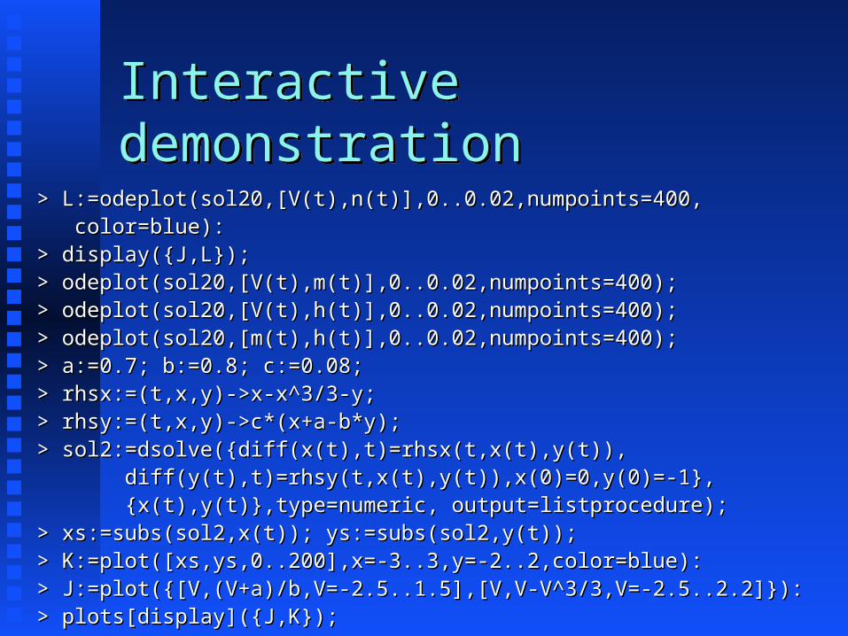
> L:=odeplot(sol20,[V(t),n(t)],0..0.02,numpoints=400,> L:=odeplot(sol20,[V(t),n(t)],0..0.02,numpoints=400, color=blue):color=blue):> display({J,L});> display({J,L});> odeplot(sol20,[V(t),m(t)],0..0.02,numpoints=400);> odeplot(sol20,[V(t),m(t)],0..0.02,numpoints=400);> odeplot(sol20,[V(t),h(t)],0..0.02,numpoints=400);> odeplot(sol20,[V(t),h(t)],0..0.02,numpoints=400);> odeplot(sol20,[m(t),h(t)],0..0.02,numpoints=400);> odeplot(sol20,[m(t),h(t)],0..0.02,numpoints=400);> a:=0.7; b:=0.8; c:=0.08;> a:=0.7; b:=0.8; c:=0.08;> rhsx:=(t,x,y)->x-x^3/3-y;> rhsx:=(t,x,y)->x-x^3/3-y;> rhsy:=(t,x,y)->c*(x+a-b*y);> rhsy:=(t,x,y)->c*(x+a-b*y);> sol2:=dsolve({diff(x(t),t)=rhsx(t,x(t),y(t)),> sol2:=dsolve({diff(x(t),t)=rhsx(t,x(t),y(t)), diff(y(t),t)=rhsy(t,x(t),y(t)),x(0)=0,y(0)=-1},diff(y(t),t)=rhsy(t,x(t),y(t)),x(0)=0,y(0)=-1}, {x(t),y(t)},type=numeric, output=listprocedure);{x(t),y(t)},type=numeric, output=listprocedure);> xs:=subs(sol2,x(t)); ys:=subs(sol2,y(t));> xs:=subs(sol2,x(t)); ys:=subs(sol2,y(t));> K:=plot([xs,ys,0..200],x=-3..3,y=-2..2,color=blue):> K:=plot([xs,ys,0..200],x=-3..3,y=-2..2,color=blue):> J:=plot({[V,(V+a)/b,V=-2.5..1.5],[V,V-V^3/3,V=-2.5..2.2]}):> J:=plot({[V,(V+a)/b,V=-2.5..1.5],[V,V-V^3/3,V=-2.5..2.2]}):> plots[display]({J,K});> plots[display]({J,K});
Interactive demonstration (Fitzhugh-Nagamo (Fitzhugh-Nagamo simplification)simplification)