lectures on quantum field...

Lectures on Quantum Field TheoryChern-Simons, WZW models, Twistors, and Multigluon Scattering Amplitudes

V. P. NAIR

City College of the CUNY

BUSSTEPP-2005

Sheffield, UK

August 22-26, 2005

BUSSTEPP-2005 – p. 1/88

Outline of lectures

• Canonical quantization

• Chern-Simons theory and its quantization

• Wess-Zumino-Witten models

• A detour into the winding number

• Uses of CS and WZW theories

• Calculation of the Dirac determinant in two dimensions

• Current correlators on the complex projective space

• An introduction to twistors, supertwistors

• Relevance of twistors to YM amplitudes

BUSSTEPP-2005 – p. 2/88

Outline of lectures

• The MHV amplitudes

• The reduction of MHV amplitudes in three steps

• A brief aside on twistor strings

• The twistor formula for all Yang-Mills amplitudes

• The Landau level connection

BUSSTEPP-2005 – p. 3/88

Canonical quantization

• Action of the general form

S =

∫

Σ

d4x L(ϕr, ∂µϕr)

Σ = V × [ti, tf ]

• General variation of fields=⇒

δL =∂L∂ϕr

δϕr +∂L

∂(∂µϕr)∂µδϕr

=

[∂L∂ϕr

− ∂

∂xµ

∂L∂(∂µϕr)

]

δϕr +∂

∂xµ

(∂L

∂(∂µϕr)δϕr

)

• Variational Principle: The equations of motion are given by

the extrema of the action,viz., δS = 0, for variations which

vanish onti, tf .BUSSTEPP-2005 – p. 4/88

Canonical quantization (cont’d)

• Choose spatial boundary conditions so that∮

∂V

δϕr∂L

∂(∂iϕr)= 0

Many possibilities (Dirichlet, Neumann, periodic)

• With these conditions

δS =

∫

Σ

d4x

[∂L∂ϕr

− ∂

∂xµ

∂L∂(∂µϕr)

]

δϕr

• Equations of motion

∂L∂ϕr

− ∂

∂xµ

∂L∂(∂µϕr)

= 0

BUSSTEPP-2005 – p. 5/88


• Go back to general variation, withδϕr 6= 0 at ti, tf .

δS =

∫

Σ

d4x

[∂L∂ϕr

− ∂

∂xµ

∂L∂(∂µϕr)

]

δϕr + Θ(tf ) − Θ(ti)

Θ(t) =

∫

V

d3x∂L

∂(∂0ϕr)δϕr =

∫

V

d3x πr(~x, t) δϕr(~x, t)

Θ = Canonical 1 − form

• Phase spaceP = Set of all classical trajectories = Initial data

P = ϕr(~x, t), ∂0ϕr(~x, t) (2nd order)

= πr(~x), ϕr(~x)= ϕr(~x, t) (1st order)

BUSSTEPP-2005 – p. 6/88


• Write Θ in general as

Θ =

∫

d3x Ai(ξ, ~x) δξi(~x)

• The curl ofΘ defines thecanonical 2-formor symplectic

structureΩ

Ωij(~x, ~x′) =

δ

δξi(~x)Aj(~x

′) − δ

δξj(~x′)Ai(~x)

= ∂IAJ − ∂JAI

• The inverse ofΩ is defined by

(Ω−1)IJ ΩJK = δIK

∫

V

d3x′(Ω−1)ij(~x, ~x′) Ωjk(~x′, ~x′′) = δi

k δ(3)(x− x′′)

BUSSTEPP-2005 – p. 7/88


• ForF, G = functions on the phase space, thePoisson bracket

is defined as

F,G = (Ω−1)IJ∂IF ∂JG

=

∫

d3x d3x′ (Ω−1)ij(~x, ~x′)δF

δξi(~x)

δG

δξj(~x′)

• For phase space coordinates themselves

ξi(~x), ξj(~x′) = (Ω−1)ij(~x, ~x′)

• Can findG (generator of the transformation) such that under an

infinitesimal canonical transformation

δF = F,G = (Ω−1)IJ ∂JG ∂IF

BUSSTEPP-2005 – p. 8/88


Transformation Generator

Change ofϕr(~x)

ϕr → ϕr + ar(~x), πr → πr G =∫

Vd3x ar(~x)πr(~x)

Change ofπr(~x)

ϕr → ϕr, πr → πr + ar(~x) G = −∫

Vd3x ar(~x)ϕr(~x)

Space translations G =∫

Vd3x ai∂iϕrπr = aiPi

xi → xi + ai Pi =∫

Vd3x ∂iϕrπr

δϕr = ai∂iϕr, δπr = ai∂iπr Pi is the momentum

Time translations H =∫

Vd3x (πr∂0ϕr − L)

Lorentz transformations

δxµ = ωµνxν Mµν =∫

Vd3x (xµTν0 − xνTµ0)

BUSSTEPP-2005 – p. 9/88


Rules of quantization

• States⇐⇒ Vectors (rays) on a Hilbert spaceH〈ϕ|α〉 = Ψα[ϕ] = wave function of|α〉 in aϕ-diagonal

representation = probability amplitude for finding the field

configurationϕ(~x) in |α〉• Observables⇐⇒ Linear hermitian operators onH

Fields⇐⇒ linear operators onH, not necessarily always

hermitian or observable.

• Canonical transformation⇐⇒ Unitary transformation onHGeneratorG =⇒ operatorG onH

BUSSTEPP-2005 – p. 10/88


|α′〉 = eiG |α〉F ′ = eiG F e−iG

i δF = F G−G F = [F,G]

[φr(~x, t), φs(~x′, t)] = 0

[πr(~x, t), πs(~x′, t)] = 0

[φr(~x, t), πs(~x′, t)] = i δrs δ

(3)(x− x′)

i∂F

∂t= [F,H]

BUSSTEPP-2005 – p. 11/88

The Chern-Simons theory in 2+1 dimensions

S = − k

4π

∫

Σ×[ti,tf ]

d3x ǫµνα Tr[Aµ∂νAα + 2

3AµAνAα

]

• Gauge groupG = SU(N)

• Aµ = −itaAaµ

• ta = basis of Lie algebra,[ta, tb] = ifabctc, Tr(tatb) = 12δab.

• k is a constant,∼ coupling constant.

• Spatial manifold can be any Riemann surfaceΣ; we takeS2,

and use complex coordinates


Fµν = 0

BUSSTEPP-2005 – p. 12/88

The Chern-Simons theory (cont’d)

• Choose the gaugeA0 = 0

• Equations of motion become

∂0Az = 0, ∂0Az = 0

A = Az = 12(A1 + iA2) andA = Az = 1

2(A1 − iA2) are

independent of time

• Gauss law constraint

Fzz ≡ ∂zAz − ∂zAz + [Az, Az] = 0

• The action becomes

S = − ik

2π

∫

dt dµΣ Tr(A ∂0A− A ∂0A)

BUSSTEPP-2005 – p. 13/88


• Vary the action to get

δS = − ikπ

∫

dt dµΣ Tr(δA ∂0A− δA ∂0A) +

− ik

2π

∫

dµΣ Tr(A δA− A δA)

]tf

ti

• Canonical one-form is

Θ = − ik

2π

∫

Σ

Tr(A δA− A δA

)

• Θ defined onA, the space of gauge potentials onΣ

A = Phase space, before reduction by gauge symmetry

BUSSTEPP-2005 – p. 14/88


• Canonical two-form

ΩabAA(x, x′) = −Ωab

AA(x, x′) =ik

2πδabδ(2)(x− x′)

• Inverting the components ofΩ =⇒ commutation rules

[Aa(z), Ab(w)] = 0

[Aa(z), Ab(w)] = 0

[Aa(z), Ab(w)] =2π

kδabδ(2)(z − w)

• Gauge transformations

Ag = gAg−1 − dgg−1

≈ −(Dθ), g ≈ 1 + θ

BUSSTEPP-2005 – p. 15/88


• Generator of infinitesimal gauge transformations is

Ga =ik

2πF a

zz

• Classically,Fzz = 0 =⇒ the reduction of the phase space

• OnS2, no degrees of freedom left; on the torus,∃ a single

mode (zero mode of∂z)

• We quantize and impose Gauss law

• Wave functions∼ f(half of phase space coordinates).

Takeψ = ψ(A) (like coherent states)

Aa ψ[A] =2π

k

δ

δAaψ[A]

BUSSTEPP-2005 – p. 16/88


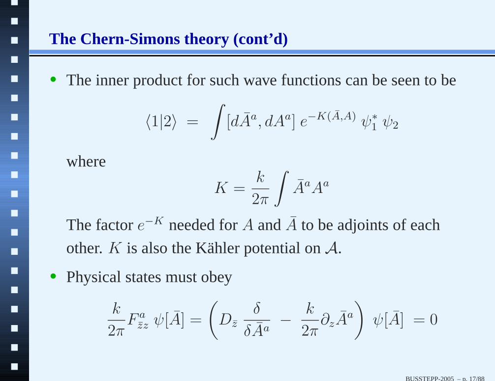
• The inner product for such wave functions can be seen to be

〈1|2〉 =

∫

[dAa, dAa] e−K(A,A) ψ∗1 ψ2

where

K =k

2π

∫

AaAa

The factore−K needed forA andA to be adjoints of each

other.K is also the Kähler potential onA.

• Physical states must obey

k

2πF a

zz ψ[A] =

(

Dzδ

δAa− k

2π∂zA

a

)

ψ[A] = 0

BUSSTEPP-2005 – p. 17/88


• Making an ansatz of the formψ = exp(k W )

DzA− ∂zA = 0, Aa =δW

δAa

• Solution is given byW = SWZW (M †) = SWZW (A).

SWZW (M †) is the Wess-Zumino-Witten action.

(To be discussed shortly)

• Wave functions are not gauge-invariant, but the inner product,

with theK[A, A]-term, is invariant.

• The coefficientk in the action is thelevel numberof the CS

theory.It must be quantized,k ∈ Z; many ways to see this.

BUSSTEPP-2005 – p. 18/88


• Under a gauge transformation,A→ Ag = gAg−1 − dgg−1.

S(Ag) = S(A) − k

4π

∫

∂M3

ǫµνTr(g−1∂µgAν) + 2πk Q[g]

• Q[g] is thewinding numberof the functiong(~x) : R3 −→ G.

Q[g] is an integer, to be discussed shortly.

• We can impose that the gauge transformationsg(~x) → 1, on

∂M3, =⇒ the surface term= 0.

(Q[g] need not be zero.)

• In a functional integral analysis, we needeiS . This will be

gauge-invariant for all transformations, including thosefor

whichQ[g] is not zero, ifk is an integer.

BUSSTEPP-2005 – p. 19/88

CS theory: problems

Problem 1. Check the inner product for the wave functions of the

CS theory by verifying thatA, A are indeed adjoints with this inner

product.

BUSSTEPP-2005 – p. 20/88

The Wess-Zumino-Witten theory

SWZW =1

8π

∫

M2

d2x√g gab Tr(∂aM ∂bM

−1) + Γ[M ]

Γ[M ] =i

12π

∫

M3

d3x ǫµνα Tr(M−1∂µM M−1∂νM M−1∂αM)

• M(x) ∈ GL(N,C) (or suitable subgroups)

• Γ[M ] = Wess-Zumino term, defined by integration overM3

with ∂M3 = M2.

• ManyM3’s with the same boundaryM2 possible≡ Different

ways to extendM(x) to M3.

• If M andM ′ are two different extensions of the same field,

thenM ′ = MN , withN = 1 onM2,

BUSSTEPP-2005 – p. 21/88

The Wess-Zumino-Witten theory (cont’d)

Γ[MN ] = Γ[M ] + Γ[N ] − i

4π

∫

M2

d2x ǫabTr (M−1∂aM ∂bNN−1)

︸︷︷︸

= 0

N = 1 on∂M3 =⇒ N is (equivalent to) a mapN : S3 → G.

Classified byΠ3[G] 6= 0, if G ⊃ any compact nonabelian Lie group.

Π3[G] =

Z SU(N), Sp(2N), Exceptionals

SO(N) for N 6= 4

Z × Z SO(4)

BUSSTEPP-2005 – p. 22/88


The winding number of the mapN(x) : S3 → G is

Q[N ] = − 1

24π2

∮

S3

d3x ǫµναTr(N−1∂µN N−1∂νN N−1∂αN)

= integer

1. Γ[N ] = 0 for N ≈ 1 ( to linear order in∂NN−1).

By successive transformations,Γ[M ] is independent of the

extension toM3 for all N connected to identity.

2. If N is homotopically nontrivial,Γ[N ] = 2πi Q[N ]

exp(−k Γ[M ]) is independent of the extension, ifk ∈ Z.

BUSSTEPP-2005 – p. 23/88


WZW theory is defined by the action

S = k SWZW , k = level number ∈ Z

In complex coordinatesz = x1 − ix2, z = x1 + ix2

SWZW =1

2π

∫

M2

Tr(∂zM∂zM−1) + Γ[M ]

SWZW [M h] = SWZW [M ]+SWZW [h]− 1

π

∫

M2

Tr(M−1∂zM ∂zh h−1)

(Polyakov-Wiegmann identity)

• Verified directly

• Chiral splitting:Antiholomorphic derivative ofM ,

holomorphic derivative ofhBUSSTEPP-2005 – p. 24/88



∂z(M−1∂zM) = M−1∂z(∂zM M−1)M = 0

• Invariances of action

M → (1 + θ(z))M M →M(1 + χ(z))

Jz = − kπ∂zM M−1 Jz = k

πM−1∂zM

∂zJz = 0 ∂zJz = 0

These follow from PW identity.

BUSSTEPP-2005 – p. 25/88


• Another important property

M −→M + δM = (1 + θ)M , θ = δM M−1 infinitesimal.

δSWZW = − 1

π

∫

Tr(∂z(δMM−1)∂zMM−1

)

= − 1

π

∫

Tr(δMM−1∂zAz)

= − 1

π

∫

Tr(δMM−1DzA)

= − 1

π

∫

Tr(A δAz)

Az = −∂zMM−1, A = −∂zM M−1,[

A 6= (Az)†

DzA = ∂zA + [Az, A]BUSSTEPP-2005 – p. 26/88


• Az andA obey the equation

∂zAz − ∂zA + [A, Az] = 0

This will be useful for evaluating Dirac determinants.

• If we useM †, we getA rather thanA.

A =δSWZW

δA

Comparing with wave function for CS theory,

ψ[A] = exp[k SWZW (M †)

]

Problem 2. Prove the Polyakov-Wiegmann identity by direct

computation.BUSSTEPP-2005 – p. 27/88

The winding number

SU(2) = The group of(2 × 2) unitary matrices of unit determinant.

Parametrizeg ∈ SU(2) as

g = φ0 + iφiσi

σ1 =

0 1

1 0

, σ2 =

0 −ii 0

, σ3 =

1 0

0 1

g† = g−1 =⇒ φ0, φi are real

det g = 1 =⇒ φ20 +

∑

i φ2i = 1

SU(2) is topologically a three-sphere,S3

SU(2)-valued functiong(x) : R3 → SU(2) ≡ R

3 → S3.

BUSSTEPP-2005 – p. 28/88

The winding number (cont’d)

If g → 1 as|~x| → ∞, R3 ∼ S3

y0 =x2 − 1

x2 + 1, yi =

2 xi

x2 + 1, y2

0 +∑

i

y2i = 1

y’s give a description ofR3 asS3; infinity → (y0 = 1, yi = 0).

Giveng(y) : S3 → SU(2), we getg(x) with g(∞) the same in all

directions. (True if we chooseg(∞) = 1.)

G =g(x) : R

3 → S3∣∣ g(x) → 1 as |~x| → ∞

=g(x) : S3 → S3

The homotopy classes (equivalence classes under smooth

deformations) of such maps =Π3[S3] = Z.

BUSSTEPP-2005 – p. 29/88


How many times is the target sphereS3 covered by the map

φµ(x) : S3x → S3 as we cover the spatialS3

x once?

Q[g] =1

vol(S3)volume traced out by φµ(x)

=1

2π2volume traced out by φµ(x)

=1

12π2

∫

d3x ǫµναβǫijkφµ∂iφ

ν∂jφα∂kφ

β

= − 1

24π2

∫

d3x Tr(g−1∂ig g

−1∂jg g−1∂kg

)ǫijk

= − 1

24π2

∫

Tr(g−1dg)3

BUSSTEPP-2005 – p. 30/88


• No metric tensor needed to define this expression. The winding

number is independent of the metric of the spatial manifold.

• Q[g1g2] = Q[g1] +Q[g2]

(g1g2)−1d(g1g2) = g−1

2 (g−11 dg1)

︸︷︷︸g2 + g−1

2 (dg2g−12 )

︸︷︷︸g2

A B

∂iAj − ∂jAi + AiAj − AjAi = 0 or dA = −A2.

Q[g1g2] = − 1

24π2

∫[TrA3 + TrB3 + (3A2B + 3B2A)

]

= Q[g1] +Q[g2] −1

8π2

∫

Tr(−dA B + AdB)

= Q[g1] +Q[g2] +1

8π2

∫

d(TrAB) = Q[g1] +Q[g2]

BUSSTEPP-2005 – p. 31/88


• Q is invariant under small deformations of the map

g(x) : S3 → SU(2); it is a topological invariant.

Q[gh] = Q[g], sinceQ[h] = 0 for h ≈ 1 + θ.

• An example of a configuration withQ = 1

g1(x) =x2 − 1

x2 + 1+ i

2xi

x2 + 1σi

(This is equivalent toφµ(x) = yµ.) g1(x) is a smooth

configuration withg1 → 1 as|~x| → ∞. It cannot be deformed

to 1 everywhere smoothly.

• Q[1] = 0, Q[g1] = 1, Q[g1g1] = 2, etc.

0 = Q[1] = Q[g†1g1] = Q[g†1] +Q[g1] = Q[g†1] + 1

=⇒ Q[g†1] = −1.BUSSTEPP-2005 – p. 32/88


Homotopy classes of mapsg(x) : S3 → S3 ∼ Additive group of integersZ.

G ⊃ SU(2) for simple, compact, nonabelian Lie groups

=⇒ Π3[G] = Z

Exception:SO(4) ∼ SU(2) × SU(2)

=⇒ Π3[SO(4)] = Z × Z

BUSSTEPP-2005 – p. 33/88


Problem 3. Consider a mapR3 → SU(2) given by

U(x) = cosF (r) + iσixi

rsinF (r)

whereF (r) is a function of the radial variabler.

This can be considered as a map fromS3 to SU(2) only if sinF is

zero atr = 0,∞; why? Using the formula for the winding number,

show that

Q[U ] =1

π(F (0) − F (∞))

BUSSTEPP-2005 – p. 34/88

Uses of CS theory

• A general relationship between CS and WZW models (Witten)

• OnS2, with no charges, all fields are gauge equivalent to zero.

=⇒ one quantum stateψ = exp[k S(M †)].

• Point charges in representationRi, the Gauss law is

ik

2πF a

zz(x) ψ =n∑

i

taRiδ(2)(x− xi) ψ

There are many physical states.

• For a conformal field theory (in two dimensions)

〈φ(z1, z1, .., zn, zn) =∑

IJ

FI(z1, · · · , zn) hIJ FJ(z1, · · · , zn)

FI(z1, · · · , zn) are called chiral blocks (conformal blocks).BUSSTEPP-2005 – p. 35/88

Uses of CS theory (cont’d)

• The wave functions of the levelk, groupG, CS theory are the

chiral blocksFI(z1, · · · , zn) for 〈φR1(x1) · · ·φRn

(xn)〉WZW .

φRi(x) = an operator corresponding to the representationRi,

of a levelk, groupG, WZW theory.

• This relation holds for higher genus Riemann surfaces. (Fora

general Riemann surface, one can have nontrivial solutionsto

Fzz = 0 even without charges.)

• CS theory and knots: Knots are classified by associating a

polynomial to each knot, or link, invariant under orientation

preserving coordinate transformations.

• The HOMFLYPT (Hoste, Ocneanu, Millet, Freyd, Lickorish,

Yetter, Przytycki, Traczyk) polynomialPL(l,m)

BUSSTEPP-2005 – p. 36/88


•

WL = Tr

[

P exp

(∮

L

itaAaµ

dxµ

dsds

)]

xµ(s), 0 ≤ s ≤ 1 = a closed curve

〈WL〉〈WU〉

≡ 1

〈WU〉

∫

dµ eiSCS(A) WL[A]

= PL[−iqN/2, i(q12 − q−

12 )]

whereq = exp(iπ/(k +N)). (N = 2 is the Jones

polynomial.)

• Theories defined by vanishing of some field strengths

DAi =∂

∂θAi+i(σµ)AAθ

Ai

∂

∂xµ, Di

A= − ∂

∂θAi

−iθAi(σµ)AA

∂

∂xµ

BUSSTEPP-2005 – p. 37/88


• N = 4 Yang-Mills theory defined by

FAiBj + FBiAj = 0

F ij

AB+ F ij

BA= 0

F j

iAB= 0

One can construct a CS-type action to obtain these.

BUSSTEPP-2005 – p. 38/88

Uses of the WZW theory

• WZW as a conformal field theory, can lead to all rational

conformal theories

• Nonabelian bosonization: ForN fermionic fields in 1+1

dimensions

ψ(iγ · ∂)ψ ⇐⇒ SWZW

]

k=1,G=U(N)

• Gauge-invariant measure for gauge fields in two dimensions

[dA]/G = dµ(M †M)︸︷︷︸

exp[2N SWZW (M †M)]

Haar measure

• The Dirac determinant in two dimensions

• Current correlators onCP1

BUSSTEPP-2005 – p. 39/88

The Dirac determinant in two dimensions

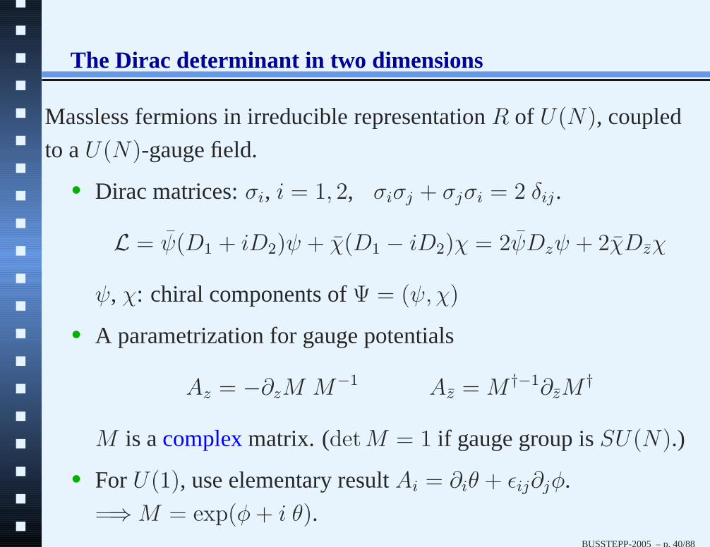
Massless fermions in irreducible representationR of U(N), coupled

to aU(N)-gauge field.

• Dirac matrices:σi, i = 1, 2, σiσj + σjσi = 2 δij.

L = ψ(D1 + iD2)ψ + χ(D1 − iD2)χ = 2ψDzψ + 2χDzχ

ψ, χ: chiral components ofΨ = (ψ, χ)

• A parametrization for gauge potentials

Az = −∂zM M−1 Az = M †−1∂zM†

M is acomplexmatrix. (detM = 1 if gauge group isSU(N).)

• ForU(1), use elementary resultAi = ∂iθ + ǫij∂jφ.

=⇒M = exp(φ+ i θ).BUSSTEPP-2005 – p. 40/88

The Dirac determinant in two dimensions (cont’d)

• Write ∂zM = −AzM ,

M(x) = 1 −∫

x′

(1

∂z

)

xx′

Az(x′)M(x′)

= 1 −∫

(∂z)−1 Az +

∫

(∂z)−1 Az(∂z)

−1 Az + · · ·

• A→ Ag = gAg−1 − dg g−1 =⇒M g = gM

• Comment: Space not simply connected→ ∃ zero modes for∂z

∃ flat potentialsa, not gauge equivalent to zero.

TorusS1 × S1. Real coordinatesξ1, ξ2, 0 ≤ ξi ≤ 1, with

ξ1 = 0 ∼ ξ1 = 1, same forξ2z = ξ1 + τξ2, τ = modular parameter

BUSSTEPP-2005 – p. 41/88


τ

Az = M

[iπ a

Im τ

]

M−1 − ∂zM M−1

• Ambiguity: M andMV (z) =⇒ sameAz. (Must ensure this

does not affect physical results)

BUSSTEPP-2005 – p. 42/88


For determinant we need regularized version of(Dz)−1

(∂z)−1xx′ = G(x, x′) =

1

π(x− x′)

Dzφ = (∂z + Az)φ = (∂z − ∂zMM−1)φ = M∂z(M−1φ) =⇒

D−1z (x, x′) =

M(x)M−1(x′)

π(x− x′)

Regularized version

D−1z (x, x′)Reg ≡ G(x, x′) =

∫

d2yM(x)M−1(y)

π(x− y)σ(x′, y; ǫ)

σ(x′, y; ǫ) =1

πǫexp

(

−|x′ − y|2ǫ

)

ǫ→0−→ δ(2)(x− x′)

BUSSTEPP-2005 – p. 43/88


Seff ≡ log detDz = Tr logDz

δSeff

δAaz(x)

= Tr[D−1

z (x, x′)(−ita)]

x′→x

= Tr [G(x, x)(−ita)]ǫ→0

G(x, x) =

∫

d2yσ(x, y)

π

[1

(x− y)−M∂zM

−1(x)

(x− y

x− y

)

−M∂zM−1 + · · ·

]

BUSSTEPP-2005 – p. 44/88


δSeff =

∫

d2xTr [G(x, x)(−ita)]ǫ→0 δAaz(x)

=1

π

∫

d2x Tr[∂zMM−1δAz

]

= − 1

π

∫

d2x Tr(A δAz)

Tr(tatb)R = AR Tr(tatb)F , AR = index of the representationR.

δSeff = −AR

π

∫

d2x Tr(A δAz)F

= AR δSWZW (M)

=⇒ detDz = det(∂z) exp[AR SWZW (M)

]

BUSSTEPP-2005 – p. 45/88


Our answer is not gauge-invariant,

δSeff = − 1

π

∫

d2x Tr(∂zAz δg g−1)

This is the two-dimensional gauge anomaly.

det(DzDz) = det(∂z∂z) exp[AR

(SWZW (M) + SWZW (M †)

)]

The gauge-invariant expression is given by

det(DzDz) = det(∂z∂z) exp[AR SWZW (M †M)

]

SWZW (M †M) = SWZW (M) + SWZW (M †)

− 1

π

∫

d2x Tr(M †−1∂zM† ∂zM M−1)

BUSSTEPP-2005 – p. 46/88


SWZW (M †M) = SWZW (M) + SWZW (M †) +1

π

∫

d2x Tr(AzAz)︸︷︷︸

local counterterm

Abelian version:

det(DzDz) = det(∂z∂z) exp

[

− 1

4π

∫

x,y

Fµν(x)G(x− y)Fµν(y)

]

G(x− y) =

∫d2p

(2π)2

1

p2exp[ip · (x− y)]

This is the fermion determinant for 2-dimensional electrodynamics

(the Schwinger model), mass term for gauge field.

BUSSTEPP-2005 – p. 47/88


Problem 4. Prove the parametrization of the gauge fields,

Az = −∂zMM−1, Az = M †−1∂M †.

(Hint: Argue that∂z + Az is invertible for a genericAz; then

constructAz which obeys

∂zAz − ∂zAz + [Az, Az] = 0

Az = (D−1z ) ∂zAz

Show that the matrixM given by

M(x, 0, C) = P exp

(

−∫ x

0 C

Azdz + Azdz

)

is independent of the path of integration and use this to construct

Az.)BUSSTEPP-2005 – p. 48/88

Current correlators of WZW on CP1

SWZW (M †) = Tr logDz − Tr log ∂z = Tr log[1 + (∂z)−1Az]

=

∞∑

n=2

(−1)n+1

n

∫d2x1

π· · · d

2xn

πTr

[Az(1)Az(2)..Az(n)

z12z23..zn1

]

(∂z)−1ij =

1

π(zi − zj), zij = zi − zj, d2x = dz dz/(−2i)

Since δSδAz

= 〈Ja〉, fromSWZW (M †), we get

〈Ja1(1)Ja2(2) · · · Jan(n)〉 =(−1)n+1

nπn

[Tr(ta1ta2 · · · tan)

z12z23 · · · zn1

+ perm′s

]

BUSSTEPP-2005 – p. 49/88

Current correlators of WZW on CP1 (cont’d)

Complex projective space of (complex) dimension1 = CP1 (= S2)

u =

α

β

Make the identificationu ∼ λu, λ ∈ C − 0. =⇒ CP1.

• A local set of coordinates:z = β/α, valid everywhere except

nearα = 0. Nearα = 0, we can usez = α/β

• The groupSL(2,C) acts onu asu→ gu, g ∈ SL(2,C),

u′ =

α′

β′

= g u =

c d

a b

α

β

, bc− ad = 1

BUSSTEPP-2005 – p. 50/88

Current correlators of WZW on CP1 (cont’d)

• At the level of the local coordinates,

z → z′ =a+ bz

c+ dz, Fractional linear transformation

• An SL(2,C)-invariant scalar product of twou’s:

(u1u2) = ǫABuA1 u

B2 = (α1β2 − α2β1) = α1α2

(β2

α2

− β1

α1

)

= −α1α2(z1 − z2) = −α1α2 z12

• Writing J = α2J , we get global expression for current

correlators

〈J a1(1) · · · J an(n)〉 = − 1

nπn

[Tr(ta1..tan)

(u1u2) (u2u3)..(unu1)+ perm′s

]

BUSSTEPP-2005 – p. 51/88

Twistors: a short introduction

Two-dimensional Laplace equation

∂ ∂ f = 0, =⇒ f(x) = h(z) + g(z)

Can we do an analogous trick for a four-dimensional problem,say,

the Dirac or Laplace equations onS4 or even onR4?

Problem: There is no natural way of combining coordinates

z1

z2

=

x1 + ix2

x3 + ix4

, or

z′1

z′2

=

x1 + ix3

x2 + ix4

or, in fact, an infinity of other choices.

Any particular choice will destroy the overallO(4)-symmetry.

How many inequivalent choices can be made, subject to, say,

preservingx2 = z1z1 + z2z2? BUSSTEPP-2005 – p. 52/88

Twistors: a short introduction (cont’d)

Given one choice, get another choice byO(4) rotation ofxµ. An

U(2)-transformation of(z1, z2) =⇒ a new combination of thez’s

preserving holomorphicity.

Inequivalent choices of

local complex structures

=

O(4)

U(2)= S2 = CP

1

S4 ∪ Set of local complex structures at each point ∼ CP3

CP1 → CP

3

↓S4

BUSSTEPP-2005 – p. 53/88


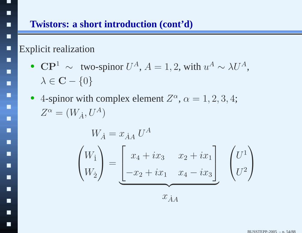
Explicit realization

• CP1 ∼ two-spinorUA, A = 1, 2, with uA ∼ λUA,

λ ∈ C − 0• 4-spinor with complex elementZα, α = 1, 2, 3, 4;

Zα = (WA, UA)

WA = xAA UA

W1

W2

=

x4 + ix3 x2 + ix1

−x2 + ix1 x4 − ix3

︸︷︷︸

U1

U2

xAA

BUSSTEPP-2005 – p. 54/88


• Complex coordinates areW1,W2, specified by the choice of

UA, a point onCP1.

• AlsoZα ∼ λZα =⇒ Zα defineCP3

• A, A, correspond toSU(2) spinor indices, right and left, in the

splittingO(4) ∼ SU(2)L × SU(2)R.

• Zα are called twistors.

• There is oneO(4)-invariant holomorphic differential,

U · dU = ǫABUAdUB.

• Do a contour integration with this to obtainO(4)-invariant

results.

f(Z) = a holomorphic function on some region in twistor

space.BUSSTEPP-2005 – p. 55/88


fA1A2···An(x) =

∮

C

U · dU UA1UA2 · · ·UAn f(Z)

• Degree of homogeneity off(Z) = −n− 2, so that integrand

is invariant underZα → λZα, UA → λUA

• Act with the chiral Dirac operatorǫCA1∇BC :

ǫCA1∇BC fA1A2···An = ǫCA1

∮

C

U · dU UA1 · · ·UAn ∇BCf(Z)

= ǫCA1

∮

C

U · dU UA1 · · ·UAn UC ∂f(Z)

∂WB

= 0

sinceǫCA1UCUA1 = 0 by antisymmetry.

BUSSTEPP-2005 – p. 56/88


• fA1A2···An(x) is a solution to the chiral Dirac equation in four

dimensions.

• Similarly, another set of solutions is

gA1A2···An(x) =

∮

C

U · dU ∂

∂WA1

∂

∂WA1

· · · ∂

∂WA1

g(Z)

g(Z) has degree of homogeneity equal ton− 2.

ǫBA1∇BB gA1A2···An = 0

• fA1A2···An(x) andgA1A2···An(x), give a complete set of

solutions to the chiral Dirac equation in four dimensions.

(Penrose’s theorem. (The theorem is much more general))

BUSSTEPP-2005 – p. 57/88


An explicit example

Considerf(Z) = 1/(a ·W b ·W c · U)

a ·W = aAxAAUA ≡ U1w2 − U2w1, b ·W = U1v2 − U2v1.

ψA =

∮

U · dU UA

a ·W b ·W c · U

=

∮

dzUA

U1

1

(w2 − zw1)(v2 − zv1)(c2 − zc1)

z = U2/U1. Take contour to enclose the pole atw2/w1:

ψA = ǫAB aAxAB

x2 w · c1

a · b =xAB

x2(axc)

ǫABaA

a · b

whereaxc = aAxAAcA. (We takea · b 6= 0.)

BUSSTEPP-2005 – p. 58/88


Conformal transformations

• Zα as a4-dim. representation ofSU(4):

Zα −→ Z ′α = (gZ)α = gαβ Z

β, g ∈ SU(4).

• Generators are:

JAB = UA∂

∂UB+ UB

∂

∂UASUL(2)

JAB = UA

∂

∂U B+ UB

∂

∂U ASUR(2)

PAA = UA ∂

∂WA

Translation

KAA = WA

∂

∂UASpecial conformal transfn.

D = WA

∂

∂WA

− UA ∂

∂UADilatation

BUSSTEPP-2005 – p. 59/88


• SU(4) ∼ Euclidean conformal group, realized in a linear and

homogeneous fashion onZα.

• For holomorphic functions, one can also choose the Minkowski

signature=⇒ SU(2, 2).

Supertwistors

AddN fermionic or Grassman coordinatesξi, i = 1, 2, ...,N=⇒ supertwistor space, parametrized by

(Zα, ξi), with Zα ∼ λZα, ξi ∼ λξi, λ ∈ C − 0

Supertwistor space isCP3|N . (λ is bosonic)

BUSSTEPP-2005 – p. 60/88


N = 4 is special=⇒ top-rank holomorphic form

Ω =1

4!ǫαβγδZ

αdZβdZγdZδ dξ1dξ2dξ3dξ4

Calabi-Yau Theorem: For a given complex structure and

Kähler class on a Kähler manifold, there exists a unique

Ricci flat metric if and only if the first Chern class of the

manifold vanishes or if and only if there is a globally

defined top-rank holomorphic form on the manifold.

Calabi-Yau supermanifold⇐⇒ a globally defined top-rank

holomorphic differential form

CP3|4 is a Calabi-Yau supermanifold.

BUSSTEPP-2005 – p. 61/88


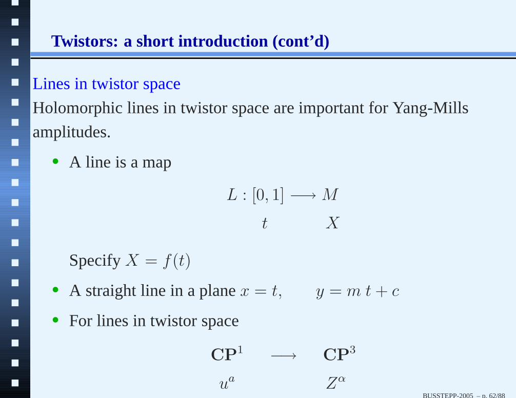
Lines in twistor space

Holomorphic lines in twistor space are important for Yang-Mills

amplitudes.

• A line is a map

L : [0, 1] −→M

t X

SpecifyX = f(t)

• A straight line in a planex = t, y = m t+ c

• For lines in twistor space

CP1 −→ CP

3

ua Zα

BUSSTEPP-2005 – p. 62/88


• =⇒ Zα = fα(u)

UA = (a−1)Aa u

a, WA = (b−1)Aaua

UseSL(2,C) transformations onua to seta = 1,

UA = uA, WA = xAAuA

• xAA ∼ Moduli of the line (placement and orientation of line)

• For supertwistors

UA = uA, WA = xAAuA

ξα = θαAu

A

Moduli = (xAA, θαA)

BUSSTEPP-2005 – p. 63/88


• Higher degree curves

Zα =∑

a

aαa1a2···ad

ua1ua2 · · · uad

ξα =∑

a

γαa1a2···ad

ua1ua2 · · · uad

Moduli = aαa1a2···ad

, γαa1a2···ad

• Symmetry ina1, a2, ..., an, =⇒ 4(d+ 1) a’s, γ’s

• Z ∼ λZ, ξ ∼ λξ =⇒aα

a1a2···ad∼ λ aα

a1a2···ad, γα

a1a2···ad∼ λ γα

a1a2···ad

• Moduli space of the curves∼ CP4d+3|4d+4. ( Can use

SL(2,C) to fix three of them.)

BUSSTEPP-2005 – p. 64/88

Why are twistors interesting?

• Twistor string theory

• A weak coupling version of the AdS/CFT duality

(Witten)

• Calculation of gauge theory amplitudes

• Quantum Chromodynamics (SU(3) gauge theory):

Amplitudes are interesting, there is a real need for them.

αs = 0.120 ±0.002 ±0.004 (jets in e−p)= 0.1224 ±0.002 ±0.005 (γ−prod. of jets)

(expt.) (theory)

Theoretical uncertainty can affect hadronic background

analysis at LHC, unification scale, etc.

BUSSTEPP-2005 – p. 65/88

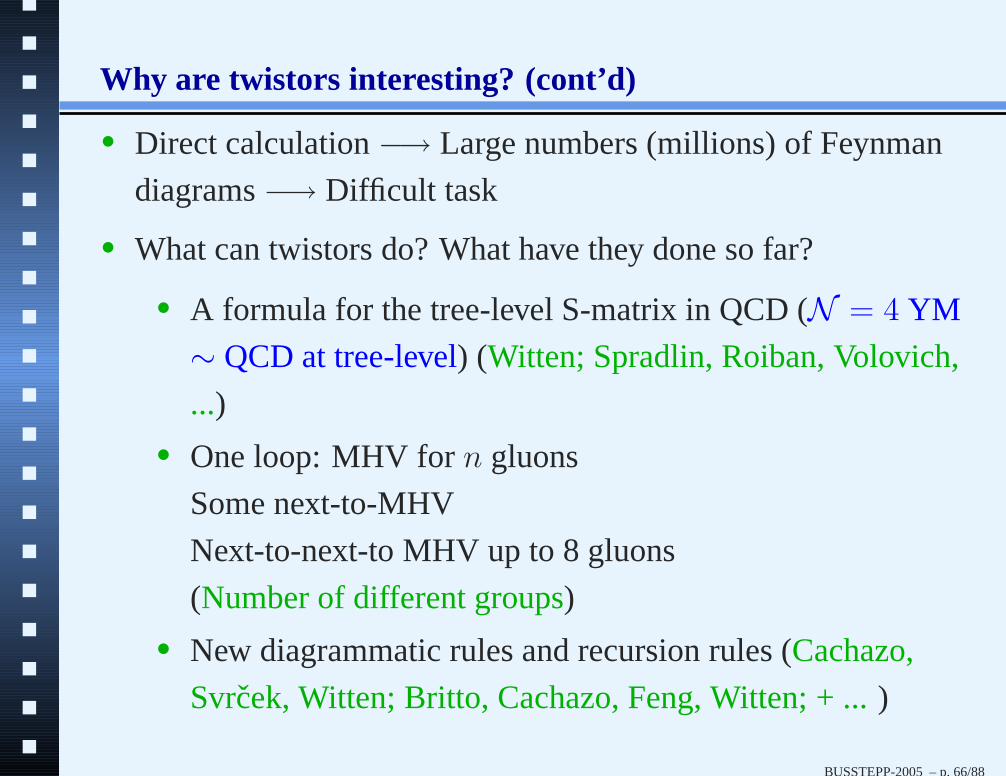
Why are twistors interesting? (cont’d)

• Direct calculation−→ Large numbers (millions) of Feynman

diagrams−→ Difficult task

• What can twistors do? What have they done so far?

• A formula for the tree-level S-matrix in QCD (N = 4 YM

∼ QCD at tree-level) (Witten; Spradlin, Roiban, Volovich,

...)

• One loop: MHV forn gluons

Some next-to-MHV

Next-to-next-to MHV up to 8 gluons

(Number of different groups)

• New diagrammatic rules and recursion rules (Cachazo,

Svrcek, Witten; Britto, Cachazo, Feng, Witten; + ...)

BUSSTEPP-2005 – p. 66/88

The MHV amplitudes

(MaximallyHelicity Violating amplitudes)

Gluons are massless,pµ ⇒ p2 = 0 ⇒ pµ is a null vector.

pAA

= (σµ)AApµ =

p0 + p3 p1 − ip2

p1 + ip2 p0 − p3

= πAπA

(π, eiθπ) −→ samepµ, pµ is real⇒ πA = (πA)∗

π =1√

p0 − p3

p1 − ip2

p0 − p3

, π =1√

p0 − p3

p1 + ip2

p0 − p3

For every momentum for a massless particle−→ a spinor

momentumπ.

BUSSTEPP-2005 – p. 67/88

The MHV amplitudes (cont’d)

Problem 5. Show that the momentum of a massless particle can be

written as a product of spinors

pAA

= πAπA

BUSSTEPP-2005 – p. 68/88


• Lorentz transformation

πA → π′A = (gπ)A = gAB πB, g ∈ SL(2,C)

• Lorentz-invariant scalar product

〈12〉 = π1 · π2 = ǫAB πA1 πB

2

• Gluon helicity

ǫµ = ǫAA =

πAλA/π · λ +1 helicity

λAπA/π · λ −1 helicity

Write amplitudes in terms of these invariantsBUSSTEPP-2005 – p. 69/88


Results obtained in 1986 byParke and Taylor, proved byBerends

and Giele

A(1a1

+ , 2a2

+ , 3a3

+ , · · · , nan+ ) = 0

A(1a1

− , 2a2

+ , 3a3

+ , · · · , nan+ ) = 0

A(1a1

− , 2a2

− , 3a3

+ , · · · , nan+ ) = ign−2(2π)4δ(p1 + ...+ pn) M

+ noncyclic permutations

M(1a1

− , 2a2

− , 3a3

+ , · · · , nan

+ ) = 〈12〉4 Tr(ta1ta2 · · · tan)

〈12〉〈23〉 · · · 〈n− 1 n〉〈n1〉

We will rewrite this in three steps

BUSSTEPP-2005 – p. 70/88

The first step: The Dirac determinant

Tr logDz = Tr log(∂z + Az)

= Tr log(

1 + 1∂zAz

)

+ constant

Tr logDz =∑

n

∫d2x1

π

d2x2

π· · · (−1)n+1

n

Tr[Az(1) · · ·Az(n)]

z12 z23 · · · zn−1n zn1

(1

∂z

)

12

=1

π(z1 − z2)=

1

π z12

z’s ∼ local coordinates onCP1.

CP1 = ua, a = 1, 2, | ua ∼ ρua , ua =

α

β

, ρ 6= 0

BUSSTEPP-2005 – p. 71/88

The first step: The Dirac determinant (cont’d)

z = β/α on coordinate patch withα 6= 0

z1 − z2 =β1

α1

− β2

α2

=β1α2 − β2α1

α1α2

=ǫabu

a1u

b2

α1α2

=u1 · u2

α1α2

Defineα2Az = A

Tr logDz = −∑ 1

n

∫Tr[A(1)A(2) · · · A(n)]

(u1 · u2)(u2 · u3) · · · (un · u1)

If ua → πA, the denominators are right for YM amplitudes.

BUSSTEPP-2005 – p. 72/88

The second step: Helicity factors

• Lorentz generator

JAB =1

2

(

πA∂

∂πB+ πB

∂

∂πA

)

, πA = ǫABπB

• Spin operatorSµ ∼ ǫµναβJναpβ, Jµν = Lorentz generator

⇒ SAA = JAB πBπA = −pA

As

• Helicity

s = −1

2πA ∂

∂πA

= −1

2degree of homogeneity in πA

Consistent with powers ofπ in amplitude

BUSSTEPP-2005 – p. 73/88

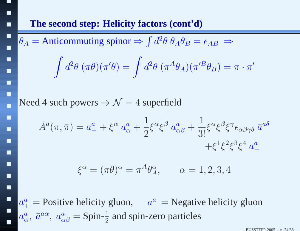
The second step: Helicity factors (cont’d)

θA = Anticommuting spinor⇒∫d2θ θAθB = ǫAB ⇒

∫

d2θ (πθ)(π′θ) =

∫

d2θ (πAθA)(π′BθB) = π · π′

Need 4 such powers⇒N = 4 superfield

Aa(π, π) = aa+ + ξα aa

α +1

2ξαξβ aa

αβ +1

3!ξαξβξγǫαβγδ a

aδ

+ξ1ξ2ξ3ξ4 aa−

ξα = (πθ)α = πAθαA, α = 1, 2, 3, 4

aa+ = Positive helicity gluon, aa

− = Negative helicity gluon

aaα, a

aα, aaαβ = Spin-1

2and spin-zero particles

BUSSTEPP-2005 – p. 74/88

Rewriting the MHV amplitude

Gauge potential for Dirac determinant

A = g taAa exp(ip · x)

Γ[A] =1

g2

∫

d8θd4x Tr logDz

]

ua→πA

MHV amplitude is

A(1a1

− , 2a2

− , 3a3

+ , · · · , nan

+ )

= i

[δ

δaa1

− (p1)

δ

δaa2

− (p2)

δ

δaa3

+ (p3)· · · δ

δaan+ (pn)

Γ[a]

]

a=0

(Nair, 1988)

BUSSTEPP-2005 – p. 75/88

An alternate representation

exp(iη · ξ) = 1 + iη · ξ +1

2!iη · ξ iη · ξ +

1

3!iη · ξ iη · ξ iη · ξ

+1

4!iη · ξ iη · ξ iη · ξ iη · ξ

η · ξ = ηαξα, state of particle= |π, η〉

A = g taaa exp(ip · x+ iη · ξ)

Amplitudes∼ coefficient ofan in Γ[A]

For1 and2 of negative helicity, choose the coefficient of

η11η21η31η41 η12η22η32η42 ∼∏

α

ηα1

∏

β

ηβ2

BUSSTEPP-2005 – p. 76/88

Recalling (super)twistor space

• Twistor

Zα = (WA, UA), Zα ∼ λZα, λ 6= 0 =⇒ CP

3

• A holomorphic line in twistor space

CP1 → CP

3

ua Zα

WA = xAA uA, UA = uA

[

UA =bAb ub =uA by SL(2,C)

• Local complex coordinates onS4

xAA =

x4 + ix3 x2 + ix1

−x2 + ix1 x4 − ix3

= x4 + ixiσi

BUSSTEPP-2005 – p. 77/88

Recalling (super)twistor space (cont’d)

WA= local complex coordinates on spacetime

• Moduli space of lines

Moduli ∼ xAA

Spacetime∼ moduli space of lines in twistor space

• N = 4 supertwistor

(Zα, ξα) = ((WA, UA), ξα), Zα ∼ λZα, ξα ∼ λξα

=⇒ CP3|4 (Calabi−Yau supermanifold)

• A holomorphic line in supertwistor space

WA = xAA uA, UA = bAb u

b = uA, ξα = θαa u

a

BUSSTEPP-2005 – p. 78/88

The third step: Lines in twistor space (Witten)

exp(ip · x) = exp

(i

2πAxAAπ

A

)

= exp

(i

2πAWA

)]

uA=πA

WA = xAAuA. RegardWA as a free variable,

∫

dσ δ

(π2

π1− U2

U1

)

exp

(i

2πAπ1WA

U1

)

= exp(i

2πAxAAπ

A)

= exp(ip · x)

settingWA = xAA uA, UA = uA, σ = u2/u1, local coordinate on

CP1

BUSSTEPP-2005 – p. 79/88

THe MHV amplitudes again

A = ign−2

∫

d4xd8θ

∫

dσ1 · · · dσn

Tr(ta1 · · · tan)

(σ1 − σ2)(σ2 − σ3) · · · (σn − σ1)

∏

i

δ

(π2

i

π1i

− U2(σi)

U1(σi)

)

× exp

(i

2πA

i π1i

WA(σi)

U1(σi)+ iπ1

i ηαiξα(σi)

U1(σi)

)

+ noncyclic permutations

WA = xAA uA, UA = uA, ξα = θα

a ua

Remark: Calculate with signature(+ + −−) (real twistors) and

continue

BUSSTEPP-2005 – p. 80/88

Properties of the amplitudeA

• Holomorphic in the twistor variablesZα, ξα, holomorphic in

the variableσ or ua.

• Invariant underZα → λZα, ξα → λξα,

• Has support only on a curve of degree one in supertwistor

space

• Integration over the modulixAA, θαA

One can obtain the amplitude by taking

1. Holomorphic mapCP1 → CP

3|4, degree one

2. Pickn pointsσ1, σ2, · · · , σn

3. Evaluate the integral overσ’s, the moduli of the chosen map

BUSSTEPP-2005 – p. 81/88

Generalization to non-MHV amplitudes

Use a holomorphic map of degreed whered+ 1 is the number of

negative helicity gluons

WA(σ) = (u1)d

d∑

0

bAkσk, UA(σ) = (u1)d

d∑

0

aAk σ

k

ξα(σ) = (u1)dd∑

0

γαk σ

k

Integration over moduli

dµ =d2d+2a d2d+2b d4d+4γ

vol[GL(2,C)]

Scale invariance +SL(2,C) ⇒ GL(2,C)

(Explicit checks bySpradlin, Roiban, Volovich + others)BUSSTEPP-2005 – p. 82/88

Justification: Twistor strings (Witten)

TopologicalB-model, target spaceCP3|4

Open strings which end onD5-branes,ξα = 0, ⇒ A(Z, Z, ξ)

I =1

2

∫

Y

Ω ∧ Tr(A ∂ A +2

3A3)

Y ⊂ CP3|4, ξ = 0

Ω =1

4!ǫαβγδZ

αdZβdZγdZδ dξ1dξ2dξ3dξ4

= top−rank holomorphic form on CP3|4

Equations of motion⇒ ∂A + ... = 0

Holomorphic fields on twistor space⇒ massless fields on spacetime

(Penrose correspondence) BUSSTEPP-2005 – p. 83/88

Twistor strings (cont’d)

Effective action in spacetime

I =

∫

Tr[

GABFAB + χAαDAAχAα + · · ·

]

GAB = self-dual field, helicity−1, A ∼ helicity +1

D1-branes (instantons)⇒ +12

∫G2ǫ

Integrate this out⇒N = 4 YM with ǫ ∼ g2

〈GA〉 ∼ 1, 〈AA〉 ∼ ǫ, GAA−vertex

(d+ 1) G’s ⇒ d ǫ’s ⇒ Instanton number =d

d+ 1 negative helicity gluons⇒ Holomorphic maps of degreed

BUSSTEPP-2005 – p. 84/88

Rewriting in a compact form

Zα =∑

a

aαa1a2···ad

ua1 · · · uad , ξα =∑

a

γαa1a2···ad

ua1 · · · uad

Φ(π, π, η) =δ [Π · Z(σ)]Z(σ) · A

Π · A× exp

(i

2

Π · Z(σ) Π · AZ(σ) · A + i

Π · AZ(σ) · Aη · ξ(σ)

)

Πα = (0, πA) = (0, 0, π1, π2), Aα = (0, 0, 1, 0)

A =

∫

dµ

∫∏

i

(udu)i Φ(πi, πi, ηi)

×(

δ

δAa1(u1)· · · δ

δAan(un)

)

Tr logDz

]

A=0BUSSTEPP-2005 – p. 85/88

The Landau level connection

FieldsQ = (Zα, ξα) onCP1 + monopole of charged at the center

Zα =∑

a

aαa1a2···ad

ua1ua2 · · · uad + higher Landau levels

ξα =∑

a

γαa1a2···ad

ua1ua2 · · · uad + higher Landau levels

S =

∫

dµ(CP1)

[

q(∂ + A)q + Y (DQ)]

(Related toBerkovits’ string theory)

M =

∫

e−S =∑

d

CdAd

For A = ∂Φ(π, π, η), higher Landau levels do not contribute

BUSSTEPP-2005 – p. 86/88

Remarks

• This may help with larged limit

• Some similar structures can be identified for graviton

amplitudes

• By composing MHV vertices, new diagrammatic rules possible

• New recursion rules, very promising

BUSSTEPP-2005 – p. 87/88

Further citations

Besides citations given, important work has been done by

• Bern, Kosower, Dixon, Bena, Del Luca,...

(UCLA-SLAC-Saclay)

• Brandhuber, Spence, Travaglini, Bedford(Queen Mary)

• Khoze, Glover, Georgiou, ...(Durham)

• W. Siegel, ...

• many others

BUSSTEPP-2005 – p. 88/88

lectures on quantum field...

Documents