lectures in quantum field theory – lecture 2

Instituto Superior Tecnico

Jorge C. Romao IDPASC School Braga – 1

Lectures in Quantum Field Theory – Lecture 2

Jorge C. RomaoInstituto Superior Tecnico, Departamento de Fısica & CFTP

A. Rovisco Pais 1, 1049-001 Lisboa, Portugal

January 2014

IST Summary for Lecture 2: QED as an Example

Summary

QED as a gauge theory

Propagators & GF

How to find QED F.R.?

Coulomb scattering e−

Coulomb scattering e+

γ in internal lines

Higher Orders

γ in external lines

QED Feynman Rules

Simple Processes

Compton Scattering

e−e+ → µ−µ+

QFT Computations



Propagators and Green functions

Feynman rules for QED

Electrons and positrons in external lines

Photons in internal lines

Photons in external lines

Higher orders

Example 1: Compton scattering

Example 2: e− + e+ → µ− + µ+ in QED

IST Local invariance of Dirac equation

Summary


• Local invariance

• QED Lagrangian

Propagators & GF





Higher Orders


QED Feynman Rules

Simple Processes

Compton Scattering

e−e+ → µ−µ+

QFT Computations


We start with Dirac Lagrangian

L = ψ(i∂/−m)ψ

It is invariant under global phase transformations

ψ′ = eiαψ, α infinitesimal → δψ = iαψ, δψ = −iαψ

What happens if the transformations are local, α = α(x)?

δψ = iα(x)ψ ; δψ = −iα(x)ψ

We have then

δL = −ψγµψ ∂µα(x)

and the Lagrangian is no longer invariant

IST Local invariance of Dirac equation . . .

Summary



• QED Lagrangian

Propagators & GF





Higher Orders


QED Feynman Rules

Simple Processes

Compton Scattering

e−e+ → µ−µ+

QFT Computations


We see that the problem is connected with the fact that ∂µψ do nottransform as ψ. We are then led to the concept of covariant derivative Dµ

that transforms as the fields,

δDµψ = iα(x)Dµψ

For the Dirac field we define, in analogy with minimal prescription,

Dµ = ∂µ + ieAµ

The vector field Aµ is a field that ensures that we can choose the phaselocally. Its transformation is chosen to compensate the term proportional to∂µα

δAµ = −1

e∂µα(x)

We are then led to the introduction of the electromagnetic field Aµ

satisfying the usual gauge invariance.

IST QED Lagrangian

Summary



• QED Lagrangian

Propagators & GF





Higher Orders


QED Feynman Rules

Simple Processes

Compton Scattering

e−e+ → µ−µ+

QFT Computations


This new vector field Aµ needs a kinetic term. The only term quadratic thatis invariant under the local gauge transformations is

Fµν = ∂µAµ − ∂νAµ, δFµν = 0

A mass term of the form AµAµ is not gauge invariant, so the field Aµ

(photon) is massless

The final Lagrangian is

LQED = −1

4FµνF

µν + ψ(iD/−m)ψ ≡ Lfree + Linteraction

where

Lfree = −1

4FµνF

µν + ψ(i∂/−m)ψ, Linteraction = −eψγµψAµ

This Lagrangian is invariant under local gauge transformations and describesthe interactions of electrons (and positrons) with photons. The theory iscalled Quantum Electrodynamics (QED)

IST The non-relativistic propagator

Summary


Propagators & GF

•Non-relativistic Prop.

•GF as propagators

•S Matrix

•Relativistic Prop.

•New processes

•Green Function

•S Matrix elements

• In & Out states





Higher Orders


QED Feynman Rules

Simple Processes

Compton Scattering

e−e+ → µ−µ+

QFT Computations


We will follow the method of Richard Feynman to arrive at the rules forcalculations in QED.

As a warm up exercise we start with the non-relativistic Schrodinger equation

(

i∂

∂t−H

)

ψ(~x, t) = 0, H = H0 + V

where H0 is the free particle Hamiltonian

H0 = −∇2

2m

We can rewrite the equation in the form

(

i∂

∂t−H0

)

ψ = V ψ

For arbitrary V this equation can normally only be solved in perturbationtheory

IST The non-relativistic propagator . . .

Summary


Propagators & GF



•S Matrix


•New processes

•Green Function


• In & Out states





Higher Orders


QED Feynman Rules

Simple Processes

Compton Scattering

e−e+ → µ−µ+

QFT Computations


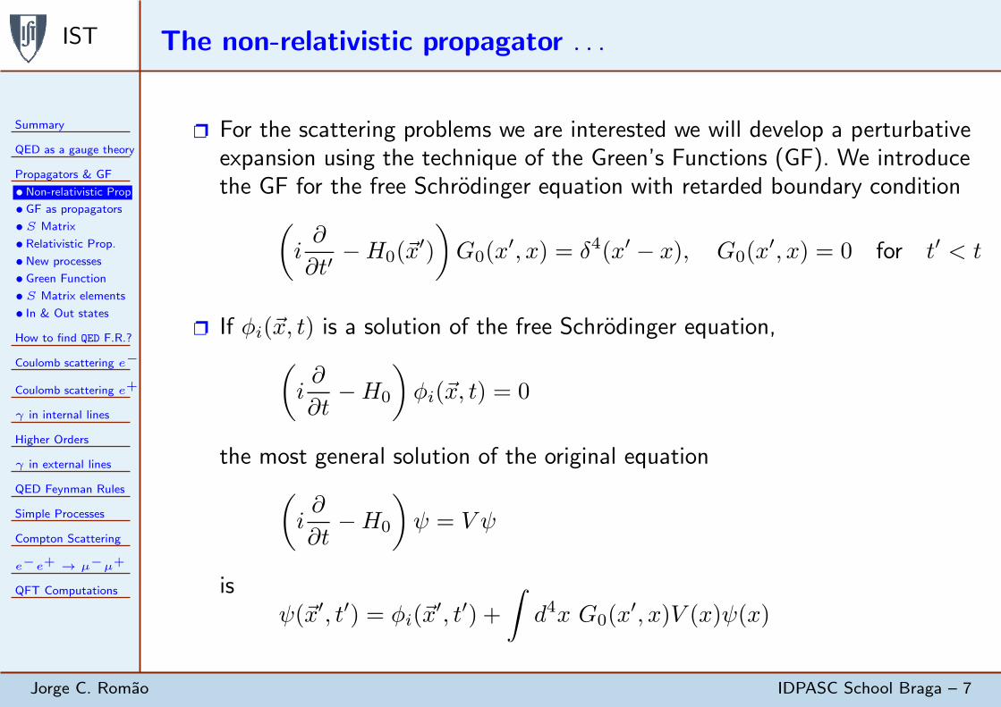
For the scattering problems we are interested we will develop a perturbativeexpansion using the technique of the Green’s Functions (GF). We introducethe GF for the free Schrodinger equation with retarded boundary condition

(

i∂

∂t′−H0(~x

′)

)

G0(x′, x) = δ4(x′ − x), G0(x

′, x) = 0 for t′ < t

If φi(~x, t) is a solution of the free Schrodinger equation,

(

i∂

∂t−H0

)

φi(~x, t) = 0

the most general solution of the original equation

(

i∂

∂t−H0

)

ψ = V ψ

isψ(~x′, t′) = φi(~x

′, t′) +

∫

d4x G0(x′, x)V (x)ψ(x)


Summary


Propagators & GF



•S Matrix


•New processes

•Green Function


• In & Out states





Higher Orders


QED Feynman Rules

Simple Processes

Compton Scattering

e−e+ → µ−µ+

QFT Computations


We can use this integral equation to establish a perturbative series. Considerthat the interaction is localized, that is V (~x, t) → 0 as t→ −∞. Then dueto the retarded GF properties we have

limt′→−∞

ψ(~x′, t′) = φi(~x′, t′)

that is in the remote past we have a plane wave.

Now if V is small (in some sense) we can solve the integral equationperturbatively

ψ(~x′, t′) =φi(~x′, t′) +

∫

d4x1 G0(x′, x1)V (x1)φi(x1)

+

∫

d4x1d4x2 G0(x

′, x1)V (x1)G0(x1, x2)V (x2)φi(x2)

+

∫

d4x1d4x2d

4x3 G0(x′, x1)V (x1)G0(x1, x2)V (x2)G0(x2, x3)V (x3)φi(x3)

+ · · ·


Summary


Propagators & GF



•S Matrix


•New processes

•Green Function


• In & Out states





Higher Orders


QED Feynman Rules

Simple Processes

Compton Scattering

e−e+ → µ−µ+

QFT Computations


We can look at the perturbative series in another way, in terms of the full

GF of the theory with interactions, G(x′, x)

(

i∂

∂t−H0(x

′)− V (x′)

)

G(x′, x) ≡ δ4(x′ − x)

It satisfies

G(x′, x) = G0(x′, x) +

∫

d4y G0(x′, y)V (y)G(y, x)

This leads to the perturbative series (small V )

G(x′, x) =G0(x′, x) +

∫

d4x1 G0(x′, x1)V (x1)G0(x1, x)

+

∫

d4x1d4x2 G0(x

′, x2)V (x2)G0(x2, x1)V (x1)G0(x1, x)

+ · · ·

IST Green Functions as Propagators

Summary


Propagators & GF



•S Matrix


•New processes

•Green Function


• In & Out states





Higher Orders


QED Feynman Rules

Simple Processes

Compton Scattering

e−e+ → µ−µ+

QFT Computations


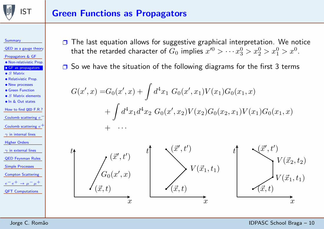
The last equation allows for suggestive graphical interpretation. We noticethat the retarded character of G0 implies x′0 > · · ·x03 > x02 > x01 > x0.

So we have the situation of the following diagrams for the first 3 terms

G(x′, x) =G0(x′, x) +

∫

d4x1 G0(x′, x1)V (x1)G0(x1, x)

+

∫

d4x1d4x2 G0(x

′, x2)V (x2)G0(x2, x1)V (x1)G0(x1, x)

+ · · ·

x

t

(~x, t)

(~x′, t′)

G0(x′, x)

x

t

(~x, t)

(~x′, t′)

V (~x1, t1)

x

t

(~x, t)

(~x′, t′)

V (~x1, t1)

V (~x2, t2)

IST Scattering processes and the S Matrix

Summary


Propagators & GF



•S Matrix


•New processes

•Green Function


• In & Out states





Higher Orders


QED Feynman Rules

Simple Processes

Compton Scattering

e−e+ → µ−µ+

QFT Computations


We are interested in scattering processes. This means that in the past wehave a solution of the free equation, a plane wave with momentum ~ki

φi(~x, t) =1

(2π)3/2ei

~ki·~x−iωit

In the future (detector) we have another plane wave with momentum ~kf

φf (~x′, t′) =

1

(2π)3/2ei

~kf ·~x′−iωf t

′

The relevant quantity is S matrix element (transition amplitude)

Sfi = limt′→∞

∫

d3x′ φ∗f (~x′, t′)ψ(~x′, t′)

= limt′→∞

∫

d3x′ φ∗f (~x′, t′)

[

φi(~x′, t′) +

∫

d4x1 G0(x′, x1)V (x1)φi(x1) + · · ·

]

=δ3(~kf − ~ki) + limt′→∞

∫

d3x′d4x1 φ∗f (~x

′, t′)G0(x′, x1)V (x1)φi(x1) + · · ·

IST The propagator for the Relativistic Theory

Summary


Propagators & GF



•S Matrix


•New processes

•Green Function


• In & Out states





Higher Orders


QED Feynman Rules

Simple Processes

Compton Scattering

e−e+ → µ−µ+

QFT Computations


The starting point is the interpretation of G(x′, x) as the probabilityamplitude to propagate the particle from x to x′

G(x′, x) =G0(x′, x) +

∫

d4x1 G0(x′, x1)V (x1)G0(x1, x)

+

∫

d4x1d4x2 G0(x

′, x2)V (x2)G0(x2, x1)V (x1)G0(x1, x)

· · · The contribution of order n corresponds to the diagram

x

x

t

x1

x2x3

xn

x′ A particle is created at x, propagates tox1, interacts with the potential V (x1),propagates to x2 and so on.

This interpretation is suited to the rela-tivistic theory because of the space-timeemphasis instead of the Hamiltonian evo-lution.

IST The propagator for the Relativistic Theory: New Processes

Summary


Propagators & GF



•S Matrix


•New processes

•Green Function


• In & Out states





Higher Orders


QED Feynman Rules

Simple Processes

Compton Scattering

e−e+ → µ−µ+

QFT Computations


e− e+

x

x

t

x1

x′

e−

e−e−

e+

x

x

t

x′

1

2

3 e− e+

x

x

tx′

The existence of a positron is associated with the absence of an electron ofnegative energy

Therefore we can interpret the destruction of an positron at 3 as being thecreation of an electron of negative energy at that point

This suggests (Feynman) the possibility that the amplitude to create apositron at 1 and destroy it at 3 be related to the amplitude to create anelectron of negative energy at 3 and destroy it at 1

Then electrons of positive energy propagate to the future and electrons ofnegative energy (positrons) propagate back in time

IST The propagator for the Relativistic Theory: Green Function

Summary


Propagators & GF



•S Matrix


•New processes

•Green Function


• In & Out states





Higher Orders


QED Feynman Rules

Simple Processes

Compton Scattering

e−e+ → µ−µ+

QFT Computations


Let us then look for the GF of the Dirac equation in interaction with theelectromagnetic field

(i∂/− eA/−m)ψ(x) = 0

It is the solution of the equation

(i∂/′ − eA/−m)S′F (x

′, x) = iδ4(x′ − x)

The full GF can only be obtained in perturbation theory. For the free theorywe have

(i∂/′ −m)SF (x′, x) = iδ4(x′ − x)

Noticing that SF (x′, x) = SF (x

′ − x) and applying the Fourier transform

SF (x′ − x) =

∫

d4p

(2π)4e−ip·(x′−x)SF (p)

IST The propagator for the Relativistic Theory: Green Function . . .

Summary


Propagators & GF



•S Matrix


•New processes

•Green Function


• In & Out states





Higher Orders


QED Feynman Rules

Simple Processes

Compton Scattering

e−e+ → µ−µ+

QFT Computations


Substituting in the equation we get for SF (p)

(p/−m)SF (p) = i → SF (p) =i(p/+m)

p2 −m2, p2 6= m2

To complete the definition we need a prescription on how to deal with thesingularity. This is related with the boundary conditions we want to imposeon the GF, positive energies propagate into the future and negative energiesback in time.

The inverse Fourier transform is calculated using the residue theorem

SF (x′−x) =

∫

dp0

2π

∫

d3p

(2π)3e−ip0(x′−x)0ei~p·(~x

′−~x) i

(p0)2 − (|~p|2 +m2)

××

−√

|~p|2 +m2

√

|~p|2 +m2

Re(p0)

Im(p0)

t′ > t lower semi-planet′ < t upper semi-plane


Summary


Propagators & GF



•S Matrix


•New processes

•Green Function


• In & Out states





Higher Orders


QED Feynman Rules

Simple Processes

Compton Scattering

e−e+ → µ−µ+

QFT Computations


The localization of the poles is obtained giving a negative infinitesimal partto m2

m2 → m2 − iε

With this prescription (due to Feynman) the propagator is

SF (p) = i(p/+m)

p2 −m2 + iε, → p0 = ±

(

√

|~p|2 +m2 − iε)

We can do now the integration in p0 to obtain

SF (x′ − x) =

∫

d3p

(2π)31

2E

[

(p/+m) e−ip·(x′−x) θ(t′ − t)

+(−p/+m) eip·(x′−x) θ(t− t′)

]


Summary


Propagators & GF



•S Matrix


•New processes

•Green Function


• In & Out states





Higher Orders


QED Feynman Rules

Simple Processes

Compton Scattering

e−e+ → µ−µ+

QFT Computations


We define the normalized plane waves

ψrp(x) =

1√2E

(2π)−3/2 wr(~p) e−iεrp·x

Then we obtain

SF (x′ − x) =θ(t′ − t)

∫

d3p

2∑

r=1

ψrp(x

′)ψr

p(x)

− θ(t− t′)

∫

d3p

4∑

r=3

ψrp(x

′)ψr

p(x)

This expresses SF (x′ − x) as a sum of eigenfunctions of the free Dirac

operator. From this expression is clear that the negative energy solutions(r = 3, 4) are propagated back in time (t′ < t), while the positive energysolutions are propagated in the future (t′ > t)

IST S Matrix elements

Summary


Propagators & GF



•S Matrix


•New processes

•Green Function


• In & Out states





Higher Orders


QED Feynman Rules

Simple Processes

Compton Scattering

e−e+ → µ−µ+

QFT Computations


As we will be interested in scattering problems, we will be focusing in theelements of the S matrix. To find these we start by noticing the solution ofthe Dirac equation with interactions,

(i∂/−m)Ψ = eA/Ψ

can be written, in analogy with the non-relativistic case,

Ψ(x) = ψ(x)− ie

∫

d4y SF (x− y)A/(y)Ψ(y)

Using the expression for SF (x− y) we get

limt→+∞

Ψ(x)− ψ(x) =

∫

d3p

2∑

r=1

ψrp(x)

[

−ie∫

d4y ψr

p(y)A/(y)Ψ(y)

]

limt→−∞

Ψ(x)− ψ(x) =

∫

d3p4∑

r=3

ψrp(x)

[

+ie

∫

d4y ψr

p(y)A/(y)Ψ(y)

]

IST S Matrix elements . . .

Summary


Propagators & GF



•S Matrix


•New processes

•Green Function


• In & Out states





Higher Orders


QED Feynman Rules

Simple Processes

Compton Scattering

e−e+ → µ−µ+

QFT Computations


This again shows that positive energies are scattered into the future andnegative energy solutions in the past.

Using now the S matrix definition

Sfi = limt→εf∞

∫

d3x ψ†f (x)Ψi(x)

we get

Sfi = δfi − ieεf

∫

d4y ψf (y)A/(y)Ψi(y)

where εf = +1 for positive energies in the future (final state) and εf = −1for negative energies into the past (initial state). ψf is a plane wave with theappropriate quantum numbers for the final state.

This is the main result the we use in the following

IST Initial and Final states

Summary


Propagators & GF



•S Matrix


•New processes

•Green Function


• In & Out states





Higher Orders


QED Feynman Rules

Simple Processes

Compton Scattering

e−e+ → µ−µ+

QFT Computations


The description of initial and final states is as follows

Initial state

electron → ψi =1√2E

1√Vu(pi, si) e

−ipi·x

positron → ψi =1√2E

1√Vv(pf , sf ) e

ipf ·x

Final state

electron → ψf =1√2E

1√Vu(pf , sf ) e

−ipf ·x

positron → ψf =1√2E

1√Vv(pi, si) e

ipi·x

IST Initial and Final states

Summary


Propagators & GF



•S Matrix


•New processes

•Green Function


• In & Out states





Higher Orders


QED Feynman Rules

Simple Processes

Compton Scattering

e−e+ → µ−µ+

QFT Computations


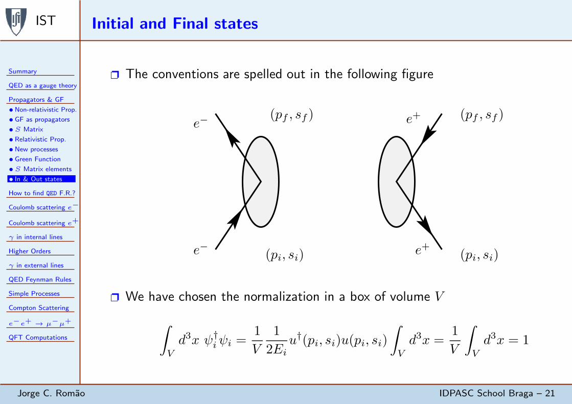
The conventions are spelled out in the following figure

e−

e− e+

e+

(pi, si)

(pf , sf )

(pi, si)

(pf , sf )

We have chosen the normalization in a box of volume V

∫

V

d3x ψ†iψi =

1

V

1

2Eiu†(pi, si)u(pi, si)

∫

V

d3x =1

V

∫

V

d3x = 1

IST How to find Feynman Rules for QED

Summary


Propagators & GF





Higher Orders


QED Feynman Rules

Simple Processes

Compton Scattering

e−e+ → µ−µ+

QFT Computations


We are going here to start from the central result

Sfi = −ieεf∫

d4yψf (y)A/ (y)Ψi(y) (i 6= f)

and derive a set of rules (Feynman Rules) that will show us how to calculatein QED

For that we will consider:

Electrons in external legs: Coulomb scattering for e−:e−+ Nuclei(Z) → e−+ Nuclei(Z)

Positrons in external legs: Coulomb scattering for e+:e++ Nuclei(Z) → e++ Nuclei(Z)

Photons in internal lines: e−µ− → e−µ−

Higher order processes: e−µ− → e−µ−

Photons in external legs: Compton scattering: γ + e− → γ + e−

IST Coulomb Scattering for Electrons

Summary


Propagators & GF



•Amplitude

•Probability

•Rate & Flux

•Cross Section

•Traces

•Theorems on traces

•Mott formula



Higher Orders


QED Feynman Rules

Simple Processes

Compton Scattering

e−e+ → µ−µ+

QFT Computations


We consider Coulomb scattering by a fixed Nuclei(Z), that is, by a classicalelectromagnetic Coulomb potential (not quantized)

A0(x) =−Ze4π|~x| ,

~A(x) = 0, e < 0

In lowest order we approximate Ψi(x) by a plane wave

Ψi(x) =1√2Ei

1√Vu(pi, si)e

−ipi·x

For the final state we take

ψf (x) =1

√

2Ef

1√Vu(pf , sf )e

ipf ·x

IST Coulomb Scattering for Electrons: The Amplitude & . . .

Summary


Propagators & GF



•Amplitude

•Probability

•Rate & Flux

•Cross Section

•Traces


•Mott formula



Higher Orders


QED Feynman Rules

Simple Processes

Compton Scattering

e−e+ → µ−µ+

QFT Computations


The S matrix amplitude between the initial and final state is

Sfi =ie2Z

4π

1

V

1√

2Ei2Ef

u(pf , sf )γ0u(pi, si)

∫

d4xei(pf−pi)·x

| ~x |

The integration can done (~q = ~pf − ~pi is the transferred momentum) and weget the final result

Sfi = iZe21

V

1√

4EiEf

u(pf , sf )γ0u(pi, si)

| ~q |2 2πδ(Ef − Ei)

We notice that we are assuming the nuclei fixed, so we have only energyconservation

The number of final states in the interval d3pf is Vd3pf

(2π)3 , and therefore the

probability for the particle to go into one of these states is

Pfi =| Sfi |2 Vd3pf(2π)3

IST Coulomb Scattering for Electrons: The Amplitude & . . .

Summary


Propagators & GF



•Amplitude

•Probability

•Rate & Flux

•Cross Section

•Traces


•Mott formula



Higher Orders


QED Feynman Rules

Simple Processes

Compton Scattering

e−e+ → µ−µ+

QFT Computations


Putting everything together we have

Pfi =Z2(4πα)2

2EiV

| u(pf , sf )γ0u(pi, si) |2| ~q |4

d3pf(2π)32Ef

[2πδ(Ef − Ei)]2

The square of the delta function needs some clarification. We define atransition time T and then

(2π)δ(Ef − Ei) = limT→∞

∫ T/2

−T/2

dtei(Ef−Ei)t

Then

2πδ(0) = limT→∞

∫ T/2

T/2

dt = limT→∞

T

Therefore

[2πδ(Ef − Ei)]2 = 2πδ(0)2πδ(Ef − Ei) = 2πTδ(Ef − Ei)

IST Coulomb Scattering for Electrons: The Transition Rate

Summary


Propagators & GF



•Amplitude

•Probability

•Rate & Flux

•Cross Section

•Traces


•Mott formula



Higher Orders


QED Feynman Rules

Simple Processes

Compton Scattering

e−e+ → µ−µ+

QFT Computations


Dividing by T we obtain the transition rate

Rfi =4Z2α2

2EiV

| u(pfsf )γ0u(pisi) |2| ~q |4

d3pf2Ef

δ(Ef − Ei)

To get the cross section we have to divide by the incident flux. Using

~Jinc = ψi(x)~γψi(x), with ψi =1√V

√Ei +m√2Ei

χ(s)

~σ·~pEi+mχ(s)

e−ipi·x

we get

| ~Jinc |=1

V

1

2Ei2 | ~pi |=

1

V

|~pi|Ei

with the usual interpretation: density, 1/V , times velocity, ~pi/Ei

IST Coulomb Scattering for Electrons: The Cross Section

Summary


Propagators & GF



•Amplitude

•Probability

•Rate & Flux

•Cross Section

•Traces


•Mott formula



Higher Orders


QED Feynman Rules

Simple Processes

Compton Scattering

e−e+ → µ−µ+

QFT Computations


The differential cross section is then

dσ

dΩ=

∫

Z2α2

| ~pi || u(pf )γ0u(pi) |2

| ~q |4p2fdpf

Efδ(Ef − Ei)

Finally using pfdpf = EfdEf we get

dσ

dΩ=Z2α2

| ~q |4 | u(pf , sf )γ0u(pi, si) |2

In practice we normally do not have polarized beams and do not measure thepolarization of the final state. So we want the unpolarized cross sectiongiven by

dσ

dΩ=

1

2

∑

si,sf

dσ

dΩ

IST Coulomb Scattering for Electrons: Sums into Traces

Summary


Propagators & GF



•Amplitude

•Probability

•Rate & Flux

•Cross Section

•Traces


•Mott formula



Higher Orders


QED Feynman Rules

Simple Processes

Compton Scattering

e−e+ → µ−µ+

QFT Computations


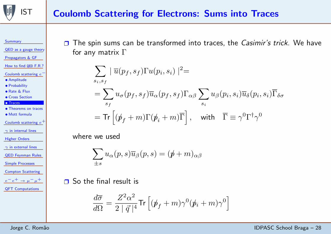
The spin sums can be transformed into traces, the Casimir’s trick. We havefor any matrix Γ

∑

si,sf

| u(pf , sf )Γu(pi, si) |2=

=∑

sf

uσ(pf , sf )uα(pf , sf )Γαβ

∑

si

uβ(pi, si)uδ(pi, si)Γδσ

= Tr[

(p/f +m)Γ(p/i +m)Γ]

, with Γ ≡ γ0Γ†γ0

where we used

∑

±s

uα(p, s)uβ(p, s) = (p/+m)αβ

So the final result is

dσ

dΩ=

Z2α2

2 | ~q |4Tr[

(p/f +m)γ0(p/i +m)γ0]

IST Theorems on traces of Dirac γ matrices

Summary


Propagators & GF



•Amplitude

•Probability

•Rate & Flux

•Cross Section

•Traces


•Mott formula



Higher Orders


QED Feynman Rules

Simple Processes

Compton Scattering

e−e+ → µ−µ+

QFT Computations


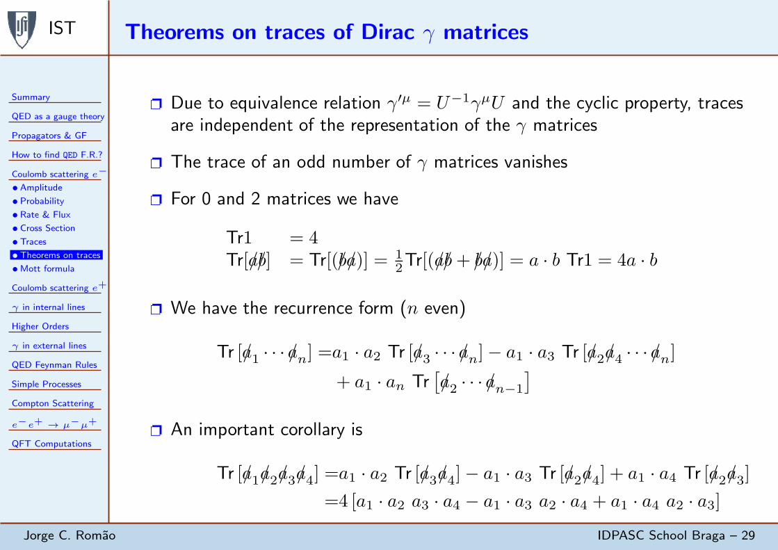
Due to equivalence relation γ′µ = U−1γµU and the cyclic property, tracesare independent of the representation of the γ matrices

The trace of an odd number of γ matrices vanishes

For 0 and 2 matrices we have

Tr1 = 4Tr[a/b/] = Tr[(b/a/)] = 1

2Tr[(a/b/+ b/a/)] = a · b Tr1 = 4a · b

We have the recurrence form (n even)

Tr [a/1 · · · a/n] =a1 · a2 Tr [a/3 · · · a/n]− a1 · a3 Tr [a/2a/4 · · · a/n]+ a1 · an Tr

[

a/2 · · · a/n−1

]

An important corollary is

Tr [a/1a/2a/3a/4] =a1 · a2 Tr [a/3a/4]− a1 · a3 Tr [a/2a/4] + a1 · a4 Tr [a/2a/3]

=4 [a1 · a2 a3 · a4 − a1 · a3 a2 · a4 + a1 · a4 a2 · a3]

IST Theorems on traces of Dirac γ matrices . . .

Summary


Propagators & GF



•Amplitude

•Probability

•Rate & Flux

•Cross Section

•Traces


•Mott formula



Higher Orders


QED Feynman Rules

Simple Processes

Compton Scattering

e−e+ → µ−µ+

QFT Computations


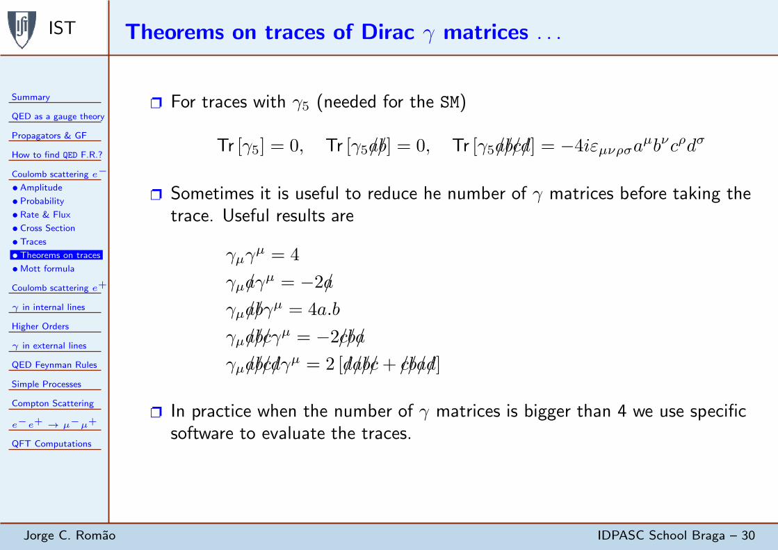
For traces with γ5 (needed for the SM)

Tr [γ5] = 0, Tr [γ5a/b/] = 0, Tr [γ5a/b/c/d/] = −4iεµνρσaµbνcρdσ

Sometimes it is useful to reduce he number of γ matrices before taking thetrace. Useful results are

γµγµ = 4

γµa/γµ = −2a/

γµa/b/γµ = 4a.b

γµa/b/c/γµ = −2c/b/a/

γµa/b/c/d/γµ = 2 [d/a/b/c/+ c/b/a/d/]

In practice when the number of γ matrices is bigger than 4 we use specificsoftware to evaluate the traces.

IST Coulomb Scattering for Electrons: The Mott Cross Section

Summary


Propagators & GF



•Amplitude

•Probability

•Rate & Flux

•Cross Section

•Traces


•Mott formula



Higher Orders


QED Feynman Rules

Simple Processes

Compton Scattering

e−e+ → µ−µ+

QFT Computations


Finally we calculate the differential cross section for Coulomb scattering

dσ

dΩ=

Z2α2

2 | ~q |4Tr[

(p/f +m)γ0(p/i +m)γ0]

The trace gives

Tr[

(p/f +m)γ0(p/i +m)γ0]

=Tr[

p/fγ0p/iγ

0]

+m2Tr[

γ0γ0]

=8EiEf − 4pi · pf + 4m2

Using (recall that E = Ei = Ej , and θ is the scattering angle)

pi ·pf = E2− | ~p |2 cos θ = m2+2β2E2 sin2 (θ/2) , | ~q |2= 4 | ~p |2 sin2 (θ/2)

We get the final result, the Mott cross section

dσ

dΩ=

Z2α2

4 | ~p |2 β2 sin4 (θ/2)

[

1− β2 sin2 (θ/2)]

in the limit β → 0 it reduces to Rutherford non-relativistic formula

IST Coulomb Scattering for Positrons

Summary


Propagators & GF





Higher Orders


QED Feynman Rules

Simple Processes

Compton Scattering

e−e+ → µ−µ+

QFT Computations


We start now from

Sfi = ie

∫

d4xψf (x)A/(x)ψi(x)

where

ψi(x) =1

√

2Ef

1√Vv(pf , sf )e

ipf ·x

ψf (x) =1√2Ei

1√Vv(pisi)e

ipi·x

e+

e+

(pi, si)

(pf , sf )

Then the S matrix element is

Sfi = −iZe2

4π

1

V

1√

2Ei 2Ef

v(pi, si)γ0v(pf , sf )

∫

d4x

| ~x |ei(pf−pi)·x

IST Coulomb Scattering for Positrons . . .

Summary


Propagators & GF





Higher Orders


QED Feynman Rules

Simple Processes

Compton Scattering

e−e+ → µ−µ+

QFT Computations


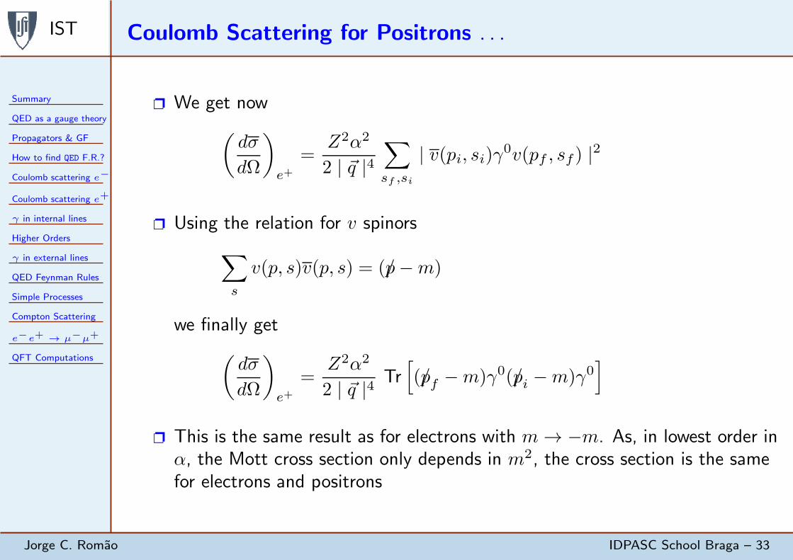
We get now

(

dσ

dΩ

)

e+=

Z2α2

2 | ~q |4∑

sf ,si

| v(pi, si)γ0v(pf , sf ) |2

Using the relation for v spinors

∑

s

v(p, s)v(p, s) = (p/−m)

we finally get

(

dσ

dΩ

)

e+=

Z2α2

2 | ~q |4 Tr[

(p/f −m)γ0(p/i −m)γ0]

This is the same result as for electrons with m→ −m. As, in lowest order inα, the Mott cross section only depends in m2, the cross section is the samefor electrons and positrons

IST Scattering e− + µ− → e− + µ−

Summary


Propagators & GF





•Photon propagator

•S Matrix

•Feynman Diagram

•Road to xs

•The Cross Section

Higher Orders


QED Feynman Rules

Simple Processes

Compton Scattering

e−e+ → µ−µ+

QFT Computations


We want now to consider the situation when the electromagnetic field is notstatic but is also quantized. As the process e− + e− → e− + e− would bringan unnecessary complication due to identical particles we choose the processwith the µ−, a kind of heavy electron interacting in the same way as the e−

We start from the fundamental relation

Sfi = −ie∫

d4xψf (x)γµψi(x)Aµ(x)

where ψi and ψf refer to the electron

We have to calculate Aµ(x). This is the field created by the muon. It isgiven by the solution of the equation (in the Lorentz gauge)

⊔⊓Aµ(x) = Jµ(x)

Jµ(x) is the current due to the muon, given by

Jµ(x) = eψµ−

f (x)γµψµ−

i (x), e < 0

IST Scattering e− + µ− → e− + µ−: Photon Propagator

Summary


Propagators & GF






•S Matrix

•Feynman Diagram

•Road to xs


Higher Orders


QED Feynman Rules

Simple Processes

Compton Scattering

e−e+ → µ−µ+

QFT Computations


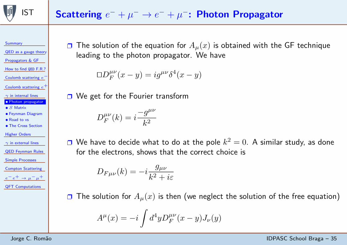
The solution of the equation for Aµ(x) is obtained with the GF techniqueleading to the photon propagator. We have

⊔⊓DµνF (x− y) = igµνδ4(x− y)

We get for the Fourier transform

DµνF (k) = i

−gµνk2

We have to decide what to do at the pole k2 = 0. A similar study, as donefor the electrons, shows that the correct choice is

DFµν(k) = −i gµνk2 + iε

The solution for Aµ(x) is then (we neglect the solution of the free equation)

Aµ(x) = −i∫

d4yDµνF (x− y)Jν(y)

IST Scattering e− + µ− → e− + µ−: S Matrix

Summary


Propagators & GF






•S Matrix

•Feynman Diagram

•Road to xs


Higher Orders


QED Feynman Rules

Simple Processes

Compton Scattering

e−e+ → µ−µ+

QFT Computations


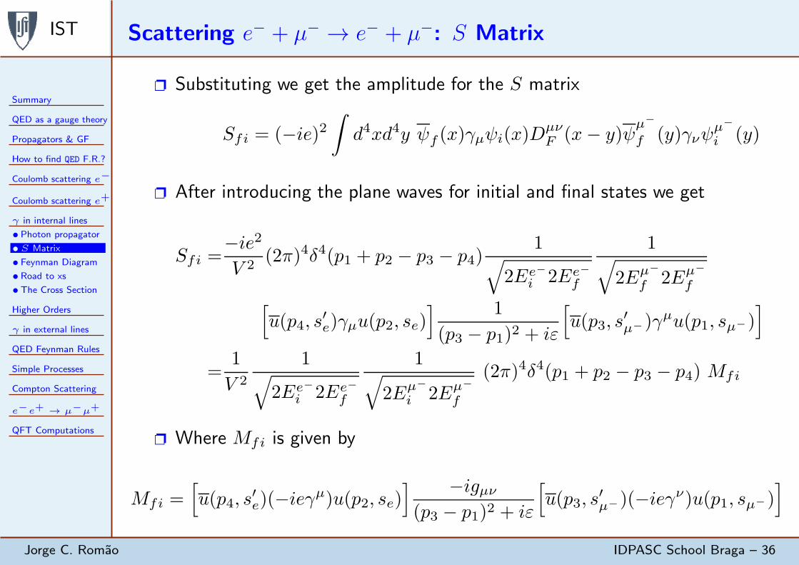
Substituting we get the amplitude for the S matrix

Sfi = (−ie)2∫

d4xd4y ψf (x)γµψi(x)DµνF (x− y)ψ

µ−

f (y)γνψµ−

i (y)

After introducing the plane waves for initial and final states we get

Sfi =−ie2V 2

(2π)4δ4(p1 + p2 − p3 − p4)1

√

2Ee−i 2Ee−

f

1√

2Eµ−

f 2Eµ−

f[

u(p4, s′e)γµu(p2, se)

] 1

(p3 − p1)2 + iε

[

u(p3, s′µ−)γµu(p1, sµ−)

]

=1

V 2

1√

2Ee−i 2Ee−

f

1√

2Eµ−

i 2Eµ−

f

(2π)4δ4(p1 + p2 − p3 − p4) Mfi

Where Mfi is given by

Mfi =[

u(p4, s′e)(−ieγµ)u(p2, se)

] −igµν(p3 − p1)2 + iε

[

u(p3, s′µ−)(−ieγν)u(p1, sµ−)

]

IST Feynman Diagram

Summary


Propagators & GF






•S Matrix

•Feynman Diagram

•Road to xs


Higher Orders


QED Feynman Rules

Simple Processes

Compton Scattering

e−e+ → µ−µ+

QFT Computations


At this point Feynman had a genius idea that completely changed the way ofmaking calculations in QFT. He made a one-to-one correspondence betweenthe matrix element

Mfi =[

u(p4, s′e)(−ieγµ)u(p2, se)

] −igµν(p3 − p1)2 + iε

[

u(p3, s′µ−)(−ieγν)u(p1, sµ−)

]

and a diagram describing the process.

p1p2

p3p4e−

e−

µ−

µ−

γ

p3 − p1e−

e−γ

(−ie γµ)time

To each fermion line entering the diagram we have a spinor u

To each fermion line leaving the diagram we have a spinor u

The internal line corresponds to the virtual (k2 6= 0) photon propagator

Each vertex corresponds to the quantity (−ieγµ), as indicated on the right

IST On the Road to the Cross Section: δ2 and Phase Space

Summary


Propagators & GF






•S Matrix

•Feynman Diagram

•Road to xs


Higher Orders


QED Feynman Rules

Simple Processes

Compton Scattering

e−e+ → µ−µ+

QFT Computations


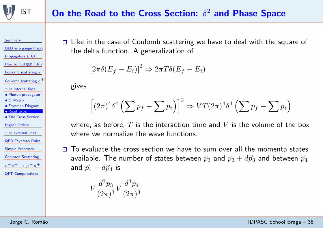
Like in the case of Coulomb scattering we have to deal with the square ofthe delta function. A generalization of

[2πδ(Ef − Ei)]2 ⇒ 2πTδ(Ef − Ei)

gives

[

(2π)4δ4(

∑

pf −∑

pi

)]2

⇒ V T (2π)4δ4(

∑

pf −∑

pi

)

where, as before, T is the interaction time and V is the volume of the boxwhere we normalize the wave functions.

To evaluate the cross section we have to sum over all the momenta statesavailable. The number of states between ~p3 and ~p3 + d~p3 and between ~p4and ~p4 + d~p4 is

Vd3p3(2π)3

Vd3p4(2π)3

IST On the Road to the Cross Section: The Incident Flux

Summary


Propagators & GF






•S Matrix

•Feynman Diagram

•Road to xs


Higher Orders


QED Feynman Rules

Simple Processes

Compton Scattering

e−e+ → µ−µ+

QFT Computations


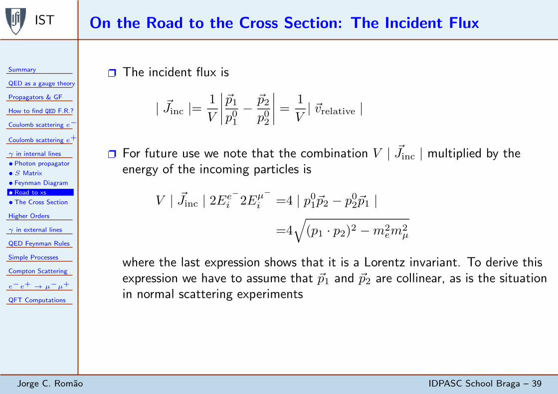
The incident flux is

| ~Jinc |=1

V

∣

∣

∣

∣

~p1p01

− ~p2p02

∣

∣

∣

∣

=1

V| ~vrelative |

For future use we note that the combination V | ~Jinc | multiplied by theenergy of the incoming particles is

V | ~Jinc | 2Ee−

i 2Eµ−

i =4 | p01~p2 − p02~p1 |

=4√

(p1 · p2)2 −m2em

2µ

where the last expression shows that it is a Lorentz invariant. To derive thisexpression we have to assume that ~p1 and ~p2 are collinear, as is the situationin normal scattering experiments

IST The Cross Section

Summary


Propagators & GF






•S Matrix

•Feynman Diagram

•Road to xs


Higher Orders


QED Feynman Rules

Simple Processes

Compton Scattering

e−e+ → µ−µ+

QFT Computations


We have now all the ingredients to evaluate the cross section. First wedetermine the transition rate by unit time and unit volume

limV,T→∞

1

V T| Sfi |2= wfi

Using the previous results we get

wfi = (2π)4δ4(p1 + p2 − p3 − p4)1

V 4

1

2p01 2p02 2p

03 2p

04

|Mfi |2

Finally we divide by the incident flux and by the number density of particlesin the target (just 1/V with our normalization) and sum over the final statesto get

σ =

∫

d3p3(2π)3

d3p4(2π)3

V 2 V

| ~Jinc |wfi

=

∫

d3p3(2π)3

d3p4(2π)3

1

2p01 2p02 2p

03 2p

04

1

V | ~Jinc |(2π)4δ4(p1 + p2 − p3 − p4) |Mfi |2

IST The Cross Section . . .

Summary


Propagators & GF






•S Matrix

•Feynman Diagram

•Road to xs


Higher Orders


QED Feynman Rules

Simple Processes

Compton Scattering

e−e+ → µ−µ+

QFT Computations


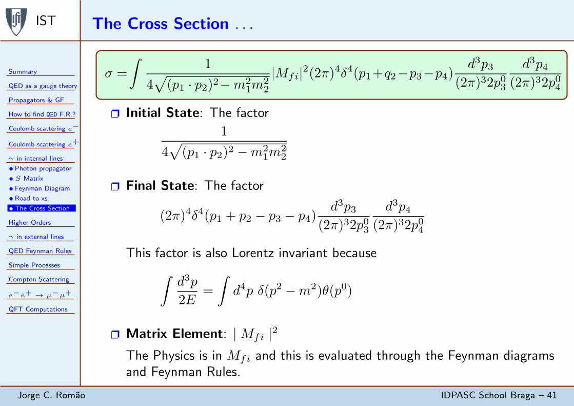
σ =

∫

1

4√

(p1 · p2)2−m21m

22

|Mfi|2(2π)4δ4(p1+q2−p3−p4)d3p3

(2π)32p03

d3p4(2π)32p04

Initial State: The factor

1

4√

(p1 · p2)2 −m21m

22

Final State: The factor

(2π)4δ4(p1 + p2 − p3 − p4)d3p3

(2π)32p03

d3p4(2π)32p04

This factor is also Lorentz invariant because

∫

d3p

2E=

∫

d4p δ(p2 −m2)θ(p0)

Matrix Element: |Mfi |2

The Physics is in Mfi and this is evaluated through the Feynman diagramsand Feynman Rules.

IST Higher Order Corrections to e−µ− → e−µ−

Summary


Propagators & GF





Higher Orders


QED Feynman Rules

Simple Processes

Compton Scattering

e−e+ → µ−µ+

QFT Computations


To have the full Feynman rules we need to know how to evaluate higherorders in perturbation theory. We go back to the master equation

Sfi = −ie∫

d4yψf (y)A/(y)Ψi(y)

Instead of the plane wave we use now the next order to Ψi, that is

Ψi(y) = −ie∫

d4xSF (y − x)A/(x)ψi(x)

and

S(2)fi =

∫

d4yd4xψf (y)(−ieγµ)SF (y − x)(−ieγν)ψi(x)Aµ(y)Aν(x)

(−ie γµ) Aµ(y)

(−ie γν) Aν(x)

IST Higher Order Corrections to e−µ− → e−µ− . . .

Summary


Propagators & GF





Higher Orders


QED Feynman Rules

Simple Processes

Compton Scattering

e−e+ → µ−µ+

QFT Computations


The origin of the terms Aµ and Aν is the current of the muon. So we shouldhave

Aµ(y)Aν(x)=

∫

d4zd4w[

DFµµ′(y−z)DFνν′(x−w)+DFµν′(y−w)DFνµ′(x−z)]

ψµ−

f (z)(−ieγµ′

)SF (z − w)(−ieγν′

)ψµ−

i (w)

This corresponds to the diagrams

y (−ie γµ′

) y (−ie γµ′

)

x (−ie γν′

) x (−ie γν′

)


Summary


Propagators & GF





Higher Orders


QED Feynman Rules

Simple Processes

Compton Scattering

e−e+ → µ−µ+

QFT Computations


Putting all together

S(2)fi =

∫

d4yd4xd4zd4w ψf (y)(−ieγµ)SF (y − x)(−ieγν)ψi(x)

[

DFµµ′(y − z)DFνν′(x− w) +DFµν′(y − w)DFνµ′(x− z)]

ψµ−

f (z)(−ieγµ′

)SF (z − w)(−ieγν′

)ψµ−

i (w)

Introducing ψi, ψf · · · and the Fourier transforms of the propagators we arelead to the final expression

S(2)fi =

1√

2Ee−i 2Ee−

f

1√

2Eµ−

i 2Eµ−

f

1

V 2(2π)4δ4(p1+ p2− p3− p4) Mfi

With

Mfi =Mafi +M b

fi


Summary


Propagators & GF





Higher Orders


QED Feynman Rules

Simple Processes

Compton Scattering

e−e+ → µ−µ+

QFT Computations


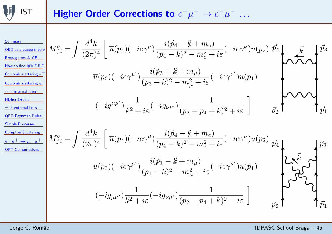
Mafi =

∫

d4k

(2π)4

[

u(p4)(−ieγµ)i(p/4 − k/+me)

(p4 − k)2 −m2e + iε

(−ieγν)u(p2)

u(p3)(−ieγu′

)i(p/3 + k/+mµ)

(p3 + k)2 −m2µ + iε

(−ieγν′

)u(p1)

(−igµµ′

)1

k2 + iε(−igνν′)

1

(p2 − p4 + k)2 + iε

]

M bfi =

∫

d4k

(2π)4

[

u(p4)(−ieγµ)i(p/4 − k/+me)

(p4 − k)2 −m2e + iε

(−ieγν)u(p2)

u(p3)(−ieγµ′

)i(p/1 − k/+mµ)

(p1 − k)2 −m2µ + iε

(−ieγν′

)u(p1)

(−igµν′)1

k2 + iε(−igνµ′)

1

(p2 − p4 + k)2 + iε

]

~p1~p2

~p3~p4 ~k

~p1~p2

~p3~p4

~k

IST Photons in external lines: Compton Scattering

Summary


Propagators & GF





Higher Orders


QED Feynman Rules

Simple Processes

Compton Scattering

e−e+ → µ−µ+

QFT Computations


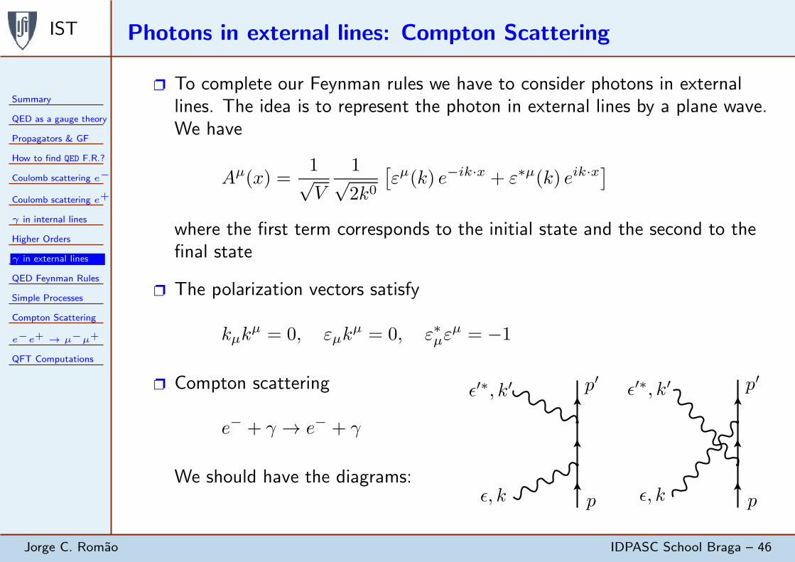
To complete our Feynman rules we have to consider photons in externallines. The idea is to represent the photon in external lines by a plane wave.We have

Aµ(x) =1√V

1√2k0

[

εµ(k) e−ik·x + ε∗µ(k) eik·x]

where the first term corresponds to the initial state and the second to thefinal state

The polarization vectors satisfy

kµkµ = 0, εµk

µ = 0, ε∗µεµ = −1

Compton scattering

e− + γ → e− + γ

We should have the diagrams:

p p

p′p′

ǫ, kǫ, k

ǫ′∗, k′ǫ′∗, k′

IST Photons in external lines: Compton Scattering . . .

Summary


Propagators & GF





Higher Orders


QED Feynman Rules

Simple Processes

Compton Scattering

e−e+ → µ−µ+

QFT Computations


The rules for the diagrams follow from the second order S(2)fi

S(2)fi =

∫

d4yd4xψf (y)(−ieQeγµ)SF (y−x)(−ieQeγ

ν)ψi(x)Aµ(y)Aν(x)

substituting Aµ(x) and Aν(y) by plane waves. For instance for diagram a)

Aµ(y) =1√V

1√2k′0

ε′∗µ eik′·y, Aν(x) =

1√V

1√2k0

ενe−ik·x

The amplitudes are then

Mafi = u(p′)(ieγµ)

i(p/+ k/+me)

(p+ k)2 −m2e

(ieγν)u(p) ε′∗µ (k′)εν(k)

M bfi = u(p′)(ieγν)

i(p/− k/+me)

(p′ − k)2 −m2e

(ieγµ)u(p) ε′∗µ (k′)εν(k)

p

p′

ǫ, k

ǫ′∗, k′

p

p′

ǫ, k

ǫ′∗, k′

IST Summary of Feynman Rules for QED

Summary


Propagators & GF





Higher Orders


QED Feynman Rules

Simple Processes

Compton Scattering

e−e+ → µ−µ+

QFT Computations


1. For a given process draw all topologically distinct diagrams

2. For each electron entering the diagram a factor u(p, s). If it leaves thediagram a factor u(p, s)

3. For each positron leaving the diagram a factor v(p, s). If it enters thediagram a factor v(p, s)

4. For each photon in the initial state a polarization vector εµ(k). In the finalstate ε∗µ(k)

5. For each electron internal line the propagator

SFαβ(p) = i(p/+m)αβp2 −m2 + iε

αβp

6. For each internal photon line the propagator (in the Feynman gauge)

DFµν(k) = −i gµνk2 + iε

µ νk

IST Summary of Feynman Rules for QED . . .

Summary


Propagators & GF





Higher Orders


QED Feynman Rules

Simple Processes

Compton Scattering

e−e+ → µ−µ+

QFT Computations


7. For each vertex the factor

(−ieQeγµ)αβ

e−

e−γ

8. For each internal momentum not fixed by energy-momentum conservation(in loops) a factor

∫

d4q

(2π)4

9. For each loop of fermions a minus sign

10. A factor of -1 between diagrams that differ but odd permutations offermions lines

IST Simple Processes in QED

Summary


Propagators & GF





Higher Orders


QED Feynman Rules

Simple Processes

Compton Scattering

e−e+ → µ−µ+

QFT Computations


If we restrict the processes to two particles in final state the number ofprocesses is very small.

Process Comment

γ + e− → γ + e− Compton Scattering

e− + e+ → µ− + µ+ in QED

µ− + e− → µ− + e− in QED

e− + e+ → e− + e+ Bhabha Scattering

e−+ Nuclei(Z) → e−+ Nuclei(Z) +γ Bremsstrahlung

e− + e+ → γ + γ Pair Annihilation

e− + e− → e− + e− Moller Scattering

γ + γ → e− + e+ Pair Creation

γ+ Nuclei(Z) → Nuclei(Z) +e− + e+ Pair Creation

We will discuss γ + e− → γ + e− and e− + e+ → µ− + µ+ in QED

IST Compton Scattering

Summary


Propagators & GF





Higher Orders


QED Feynman Rules

Simple Processes

Compton Scattering

•Amplitudes

• Spin Sums

•Cross Section

e−e+ → µ−µ+

QFT Computations


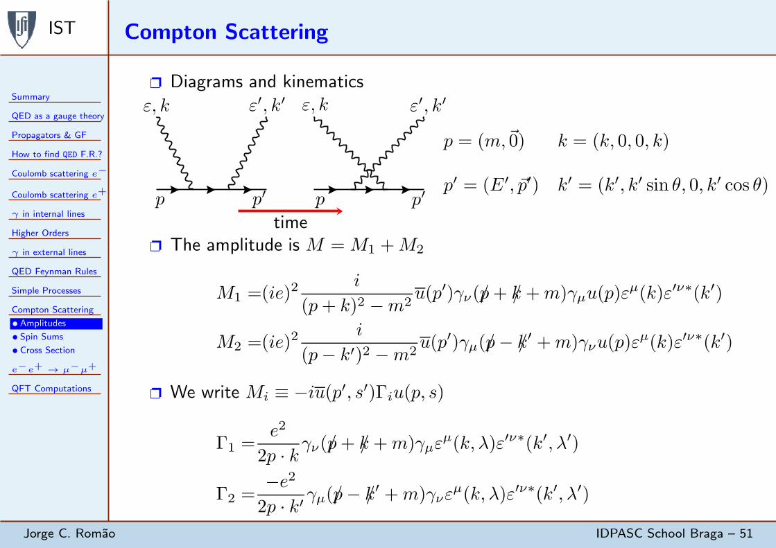
Diagrams and kinematics

pp p′p′

ε, kε, k ε′, k′ε′, k′

p = (m,~0) k = (k, 0, 0, k)

p′ = (E′, ~p′) k′ = (k′, k′ sin θ, 0, k′ cos θ)

time The amplitude is M =M1 +M2

M1 =(ie)2i

(p+ k)2 −m2u(p′)γν(p/+ k/+m)γµu(p)ε

µ(k)ε′ν∗(k′)

M2 =(ie)2i

(p− k′)2 −m2u(p′)γµ(p/− k/′ +m)γνu(p)ε

µ(k)ε′ν∗(k′)

We write Mi ≡ −iu(p′, s′)Γiu(p, s)

Γ1 =e2

2p · kγν(p/+ k/+m)γµεµ(k, λ)ε′ν∗(k′, λ′)

Γ2 =−e22p · k′ γµ(p/− k/′ +m)γνε

µ(k, λ)ε′ν∗(k′, λ′)

IST Spin Sums

Summary


Propagators & GF





Higher Orders


QED Feynman Rules

Simple Processes

Compton Scattering

•Amplitudes

• Spin Sums

•Cross Section

e−e+ → µ−µ+

QFT Computations


We want to calculate

1

4

∑

s,s′

∑

λ,λ′

|M |2 =1

4

∑

s,s′

∑

λ,λ′

[

|M1|2 + |M2|2 +M†1M2 +M1M

†2

]

We have (i = 1, 2)

Γi ≡ γ0Γ†iγ

0

∑

s,s′

|Mi|2 =∑

s,s′

u(p′, s′)Γiu(p, s)u†(p, s)Γ†

iγ0u(p′, s′)

=∑

s,s′

u(p′, s′)Γiu(p, s)u(p, s)Γiu(p′, s′)

=Tr[

(p/′ +m)Γi(p/+m)Γi

]

Where we have used

∑

s

uα(p, s)uβ(p, s) = (p/+m)αβ

IST Spin Sums . . .

Summary


Propagators & GF





Higher Orders


QED Feynman Rules

Simple Processes

Compton Scattering

•Amplitudes

• Spin Sums

•Cross Section

e−e+ → µ−µ+

QFT Computations


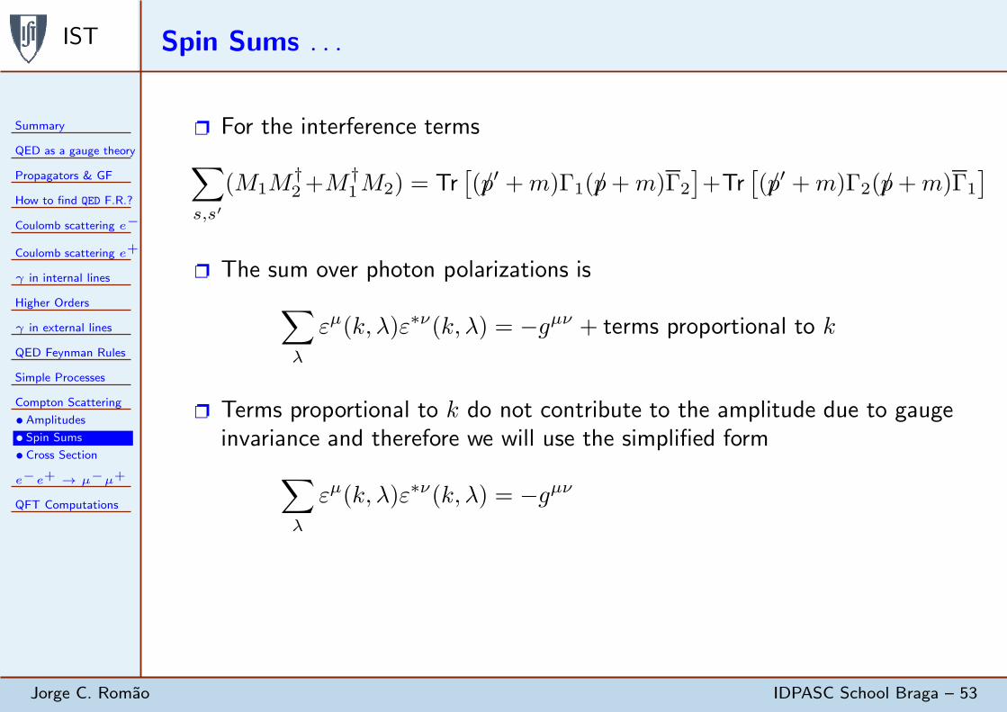
For the interference terms

∑

s,s′

(M1M†2+M

†1M2) = Tr

[

(p/′ +m)Γ1(p/+m)Γ2

]

+Tr[

(p/′ +m)Γ2(p/+m)Γ1

]

The sum over photon polarizations is

∑

λ

εµ(k, λ)ε∗ν(k, λ) = −gµν + terms proportional to k

Terms proportional to k do not contribute to the amplitude due to gaugeinvariance and therefore we will use the simplified form

∑

λ

εµ(k, λ)ε∗ν(k, λ) = −gµν

IST Compton Cross Section

Summary


Propagators & GF





Higher Orders


QED Feynman Rules

Simple Processes

Compton Scattering

•Amplitudes

• Spin Sums

•Cross Section

e−e+ → µ−µ+

QFT Computations


In the rest frame of the electron the cross section is

dσ =1

4mk(2π)4δ4(p+ k − p′ − k′)|M |2 d3p′

(2π)32p′0d3k′

(2π)32k′0

Using the delta function we integrate over d3p′. We get

dσ

dΩk′

=1

4mk

1

(2π)2

∫

dk′k′2

2k′2E′δ(m+ k − E′ − k′)|M |2

To use the last delta function we note that E′ is related to k′. In fact fromδ3(~p+ ~k − ~p ′ − ~k′) we have ~p ′ = ~k − ~k′, and therefore

E′ =√

~p ′2 +m2 =√

k2 + k′2 − 2kk′ cos θ +m2

This implies

δ(m+k−E′−k′) =δ(

k′ − k1+ k

m(1−cos θ)

)

∣

∣1 + dE′

dk′

∣

∣

withdE′

dk′=k′ − k cos θ

E′

IST Compton Cross Section . . .

Summary


Propagators & GF





Higher Orders


QED Feynman Rules

Simple Processes

Compton Scattering

•Amplitudes

• Spin Sums

•Cross Section

e−e+ → µ−µ+

QFT Computations


And therefore∣

∣

∣

∣

1 +dE′

dk′

∣

∣

∣

∣

=|E′ + k′ − k cos θ|

E′=m+ k(1− cos θ)

E′=m

E′

k

k′

Putting all together

dσ

dΩk′

=1

64π2

1

m2

(

k′

k

)2

|M |2 where |M |2 =1

4

∑

s,s′

∑

λ,λ′

|M |2

Calculating the traces

|M1|2 = 8[

2 m4 +m2(−p · p′ − p′ · k + 2p · k) + (p · k)(p′ · k)] e4

(2p · k)2

|M2|2 = 8[

2m4 +m2(−p · p′ + p′ · k′ − 2p · k′) + (p · k′)(p′ · k′)] e4

(2p · k′)2

[M1M†2 +M†

1M2] =8e4

4(k · p)(k′ · p) [2(k · p)(p · p′)− 2(k · k′)(p · p′)− 2(p · p′)(p · k′)

+m2(−2k · p− k · p′ + k · k′ − p · p′ + 2p · k′ + p′ · k′)−m4]

IST Compton Cross Section . . .

Summary


Propagators & GF





Higher Orders


QED Feynman Rules

Simple Processes

Compton Scattering

•Amplitudes

• Spin Sums

•Cross Section

e−e+ → µ−µ+

QFT Computations


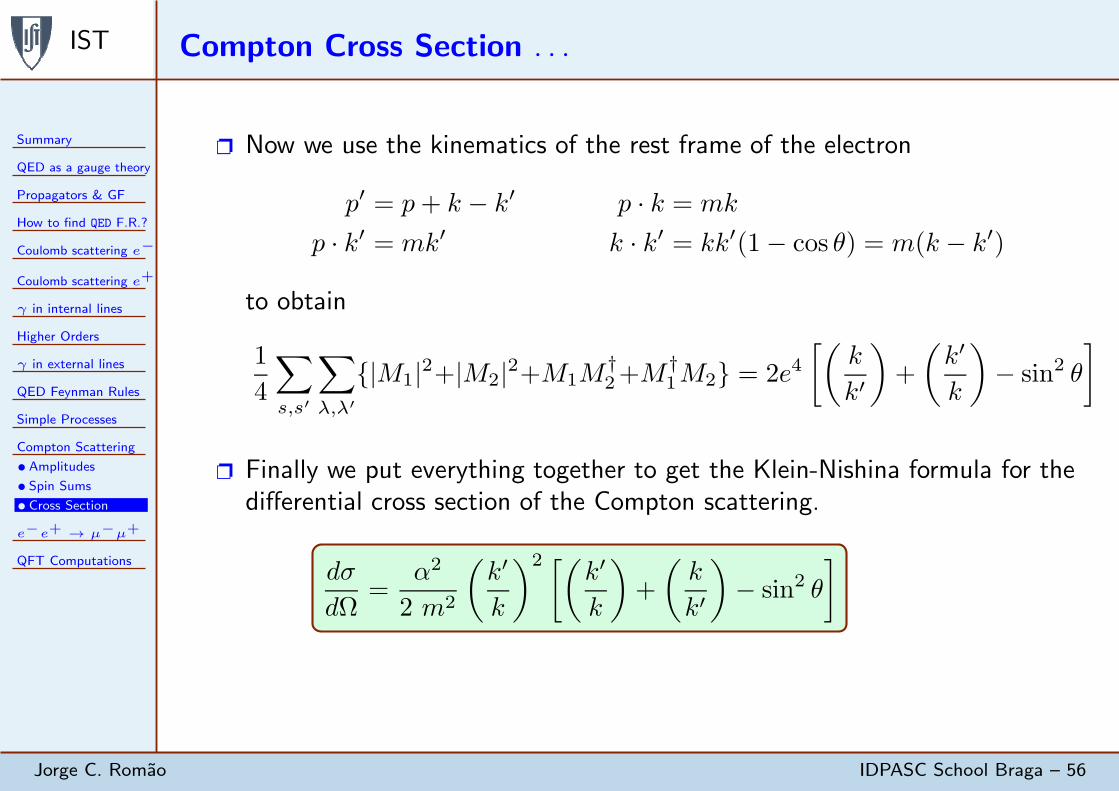
Now we use the kinematics of the rest frame of the electron

p′ = p+ k − k′ p · k = mk

p · k′ = mk′ k · k′ = kk′(1− cos θ) = m(k − k′)

to obtain

1

4

∑

s,s′

∑

λ,λ′

|M1|2+|M2|2+M1M†2+M

†1M2 = 2e4

[(

k

k′

)

+

(

k′

k

)

− sin2 θ

]

Finally we put everything together to get the Klein-Nishina formula for thedifferential cross section of the Compton scattering.

dσ

dΩ=

α2

2 m2

(

k′

k

)2 [(k′

k

)

+

(

k

k′

)

− sin2 θ

]

IST Scattering e−e+ → µ−µ+ in QED

Summary


Propagators & GF





Higher Orders


QED Feynman Rules

Simple Processes

Compton Scattering

e−e+ → µ−µ+

•Amplitude

•Cross Section

QFT Computations


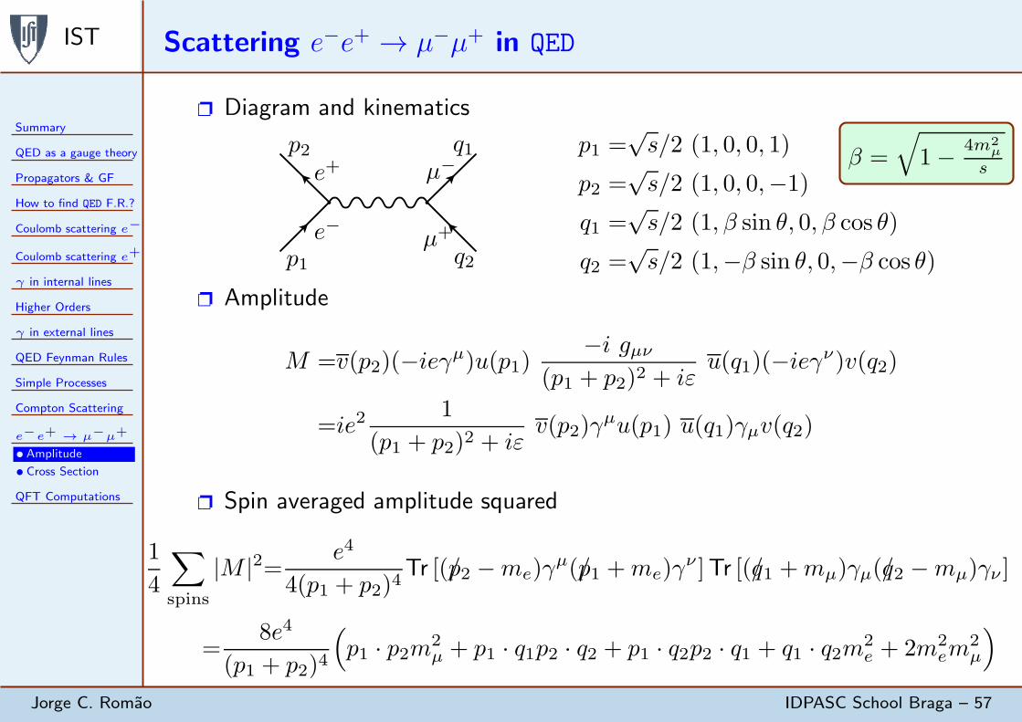
Diagram and kinematics

µ−

µ+e−

e+

p1

p2 q1

q2

p1 =√s/2 (1, 0, 0, 1)

p2 =√s/2 (1, 0, 0,−1)

q1 =√s/2 (1, β sin θ, 0, β cos θ)

q2 =√s/2 (1,−β sin θ, 0,−β cos θ)

β =

√

1− 4m2µ

s

Amplitude

M =v(p2)(−ieγµ)u(p1)−i gµν

(p1 + p2)2 + iεu(q1)(−ieγν)v(q2)

=ie21

(p1 + p2)2 + iεv(p2)γ

µu(p1) u(q1)γµv(q2)

Spin averaged amplitude squared

1

4

∑

spins

|M |2= e4

4(p1 + p2)4Tr [(p/2 −me)γ

µ(p/1 +me)γν ]Tr [(q/1 +mµ)γµ(q/2 −mµ)γν ]

=8e4

(p1 + p2)4

(

p1 · p2m2µ + p1 · q1p2 · q2 + p1 · q2p2 · q1 + q1 · q2m2

e + 2m2em

2µ

)

IST Cross Section

Summary


Propagators & GF





Higher Orders


QED Feynman Rules

Simple Processes

Compton Scattering

e−e+ → µ−µ+

•Amplitude

•Cross Section

QFT Computations


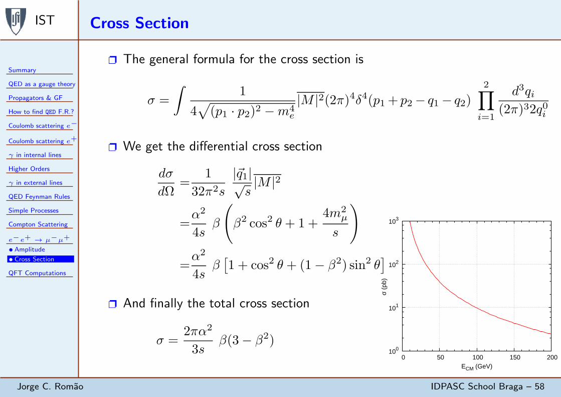
The general formula for the cross section is

σ =

∫

1

4√

(p1 · p2)2 −m4e

|M |2(2π)4δ4(p1+ p2 − q1 − q2)

2∏

i=1

d3qi(2π)32q0i

We get the differential cross section

dσ

dΩ=

1

32π2s

|~q1|√s|M |2

=α2

4sβ

(

β2 cos2 θ + 1 +4m2

µ

s

)

=α2

4sβ[

1 + cos2 θ + (1− β2) sin2 θ]

And finally the total cross section

σ =2πα2

3sβ(3− β2)

100

101

102

103

0 50 100 150 200

σ (p

b)

ECM (GeV)

IST Computational Techniques in Quantum Field Theory

Summary


Propagators & GF





Higher Orders


QED Feynman Rules

Simple Processes

Compton Scattering

e−e+ → µ−µ+

QFT Computations


Mathematica

FeynArts

Program to draw Feynman diagrams. Can be obtained fromhttp://www.feynarts.de

FeynCalc

Lorentz and Dirac algebra and calculations at one–loop. Can have asinput FeynArts. Can be obtained from http://www.feyncalc.org

QGRAF

Very efficient program to generate Feynman diagrams for any theory to anyloop order done by Paulo Nogueira. Can be downloaded fromhttp://cfif.ist.utl.pt/~paulo/qgraf.html

Numerics: C/C++ or Fortran

To do efficient numerics one has to use the power of C/C++ or Fortran. Aspecial useful package is CUBA with routines for numerical integration can beobtained from http://www.feynarts.de/cuba/

My CTQFT Home Page: http://porthos.ist.utl.pt/CTQFT/

Here you can find all the links and many programs for standard processes inQED and in the SM.

http://www.feynarts.de

http://www.feyncalc.org

http://cfif.ist.utl.pt/~paulo/qgraf.html

http://www.feynarts.de/cuba/

http://porthos.ist.utl.pt/CTQFT/

lectures in quantum field theory – lecture 2

Documents