lectures on antitrust economics chapter 3: horizontal...
TRANSCRIPT

Visit the CSIO website at: www.csio.econ.northwestern.edu. E-mail us at: [email protected].
THE CENTER FOR THE STUDY OF INDUSTRIAL ORGANIZATION
AT NORTHWESTERN UNIVERSITY
Working Paper #0041
Lectures on Antitrust Economics Chapter 3: Horizontal Mergers*
By
Michael D. Whinston
Northwestern University and NBER
* Copyright 2003, Michael D. Whinston.

Lectures on Antitrust EconomicsChapter 3: Horizontal Mergers
Michael D. Whinston∗
Draft � Comments Welcome
Contents
1 Introduction 2
2 Theoretical Considerations 22.1 The Williamson Trade-off . . . . . . . . . . . . . . . . . . . . . . . . . . . . 22.2 Formal Analyses of the Welfare Effects of Mergers . . . . . . . . . . . . . . . 6
3 The Department of Justice/FTC Merger Guidelines 143.1 Market DeÞnition . . . . . . . . . . . . . . . . . . . . . . . . . . . . . . . . . 143.2 Calculating Concentration and Concentration Changes . . . . . . . . . . . . 163.3 Evaluation of Other Market Factors . . . . . . . . . . . . . . . . . . . . . . . 173.4 Pro-competitive JustiÞcations . . . . . . . . . . . . . . . . . . . . . . . . . . 19
4 Econometric Approaches to Answering the Guidelines� Questions 204.1 DeÞning the Relevant Market . . . . . . . . . . . . . . . . . . . . . . . . . . 204.2 Evidence on the Effects of Increasing Concentration on Prices . . . . . . . . 27
5 Breaking the Market DeÞnition Mold 315.1 Merger Simulation . . . . . . . . . . . . . . . . . . . . . . . . . . . . . . . . 315.2 Residual Demand Estimation . . . . . . . . . . . . . . . . . . . . . . . . . . 355.3 The Event Study Approach . . . . . . . . . . . . . . . . . . . . . . . . . . . 39
6 Examining the Results of Actual Mergers 426.1 Price Effects . . . . . . . . . . . . . . . . . . . . . . . . . . . . . . . . . . . . 436.2 Efficiencies . . . . . . . . . . . . . . . . . . . . . . . . . . . . . . . . . . . . . 51
∗Northwestern University and NBER. Copyright 2003, Michael D. Whinston.

Lectures on Antitrust Economics Chapter 3: Horizontal Mergers 2
1 Introduction
In this chapter our attention turns to horizontal merger policy. The Sherman Act�s prohibi-
tion on �contracts, combinations, and conspiracies in restraint of trade,� whose application
to price Þxing we discussed in Chapter 2, also applies to horizontal mergers, but with an
important difference: horizontal mergers are evaluated by the courts under a Rule of Reason
analysis based on the presumption that they often have important efficiency beneÞts. In
addition, the Clayton Act�s Section 7 includes a more speciÞc prohibition on mergers where
the effect may be �substantially to lesson competition, or to tend to create a monopoly.�
Despite the potential for efficiencies arising from horizontal mergers, from the 1950�s
through the 1970�s the U.S. courts were extremely hostile toward them, often condemning
horizontal mergers in markets that were and would remain very unconcentrated.1 Since
1980, however, with a more conservative judiciary and an increasing inßuence of economic
reasoning, horizontal merger policy has become much more permissive. During this same
period, there has also been substantial progress in economists� ability to analyze proposed
horizontal mergers. In what follows we will review this progress, while also noting some of
the signiÞcant open questions that remain.
2 Theoretical Considerations
2.1 The Williamson Trade-off
The central issue in the evaluation of horizontal mergers lies in the need to balance any
reductions in competition against the possibility of productivity improvements arising from
a merger. This trade-off was Þrst articulated in the economics literature by Williamson
[1968], in a paper aimed at getting efficiencies to be taken seriously. This �Williamson
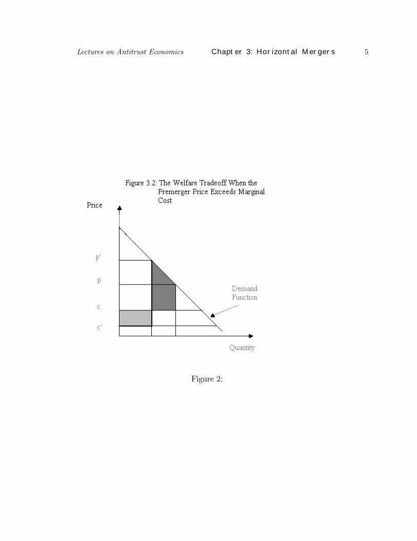
tradeoff� is illustrated in Figure 3.1.1Indeed, concern over the fate of small (and often inefficient) businesses frequently led the courts during
this period to use merger-related efficiencies as evidence against a proposed merger.

Lectures on Antitrust Economics Chapter 3: Horizontal Mergers 3
Figure 1:
Suppose that the industry is initially competitive, with a price equal to c. Suppose also
that after the merger, the marginal cost of production falls to c0 and the price rises to p0.2
Aggregate social welfare before the merger is given by the area ABC, while aggregate welfare
after the merger is given by area ADEF. Which is larger involves a comparison between the
area of the dark grey shaded triangle, equal to the deadweight loss from the post-merger
supracompetitive pricing, and the area of the light grey shaded rectangle, equal to the post-
merger cost savings (at the post-merger output level). If there is no improvement in costs,
then the area of the rectangle will be zero and the merger reduces aggregate welfare; if there
is no increase in price, then the area of the triangle will be zero, and the merger increases
2We assume here that these costs represent true social costs. Reductions in the marginal cost of productiondue to, say, increased monopsony power resulting from the merger would not count as a social gain. Likewise,if input markets are not perfectly competitive, then reductions in cost attributable to the merger must becalculated at the true social marginal cost of the inputs rather than at their distorted market prices.

Lectures on Antitrust Economics Chapter 3: Horizontal Mergers 4
aggregate welfare. Williamson�s main point was that it does not take a large decrease in
cost for the area of the rectangle to exceed that of the triangle: put crudely, one might say
that �rectangles tend to be larger than triangles�. Indeed, in the limit of small changes
in price and cost, differential calculus tells us that this will always be true: formally, the
welfare reduction from an inÞnitesimal increase in price starting from the competitive price
is of second-order (i.e., has a zero derivative), while the welfare increase from an inÞnitesimal
decrease in cost is of Þrst-order (i.e., has a strictly positive derivative).
Four important points should be noted, however, about this Williamson trade-off argu-
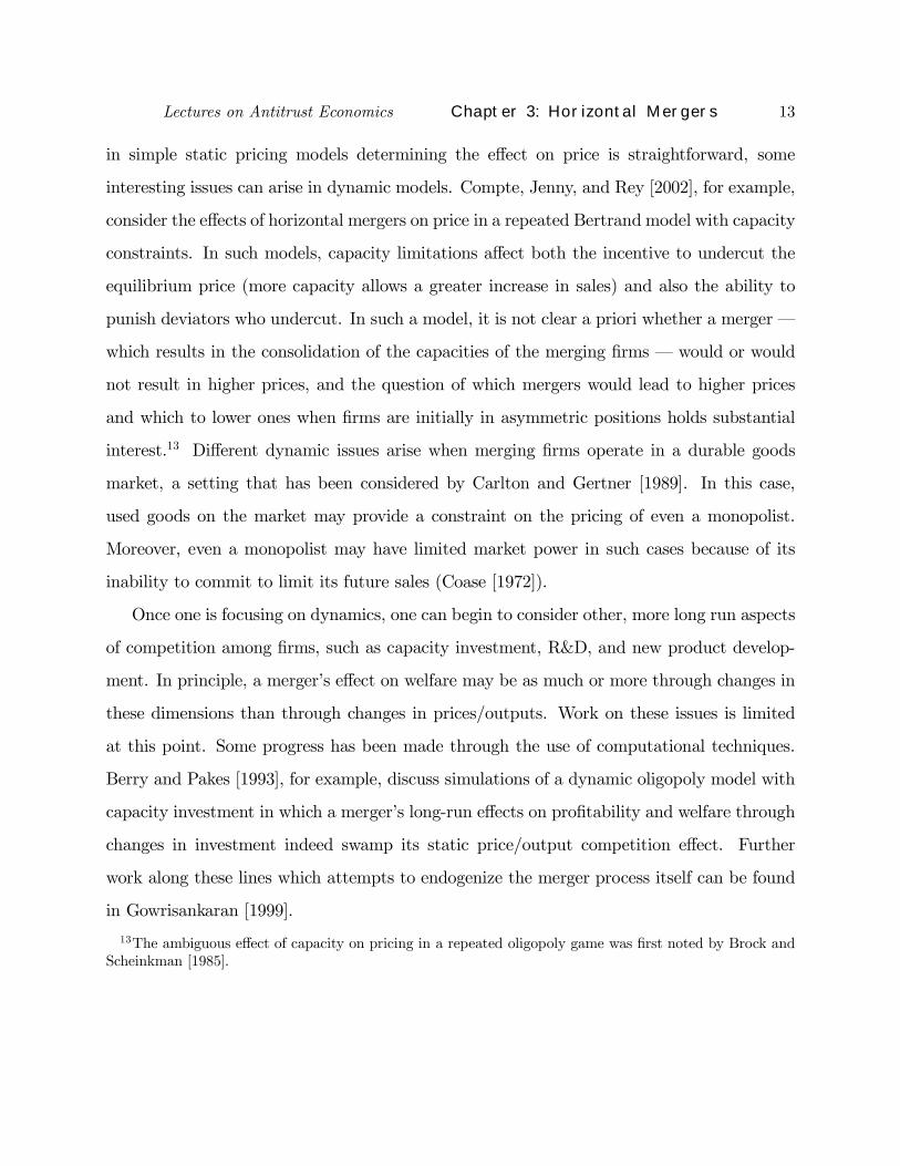
ment. First, a critical part of the argument involved the assumption that the pre-merger price
was competitive; i.e., equal to marginal cost. Without this assumption we would no longer
be comparing a triangle to a rectangle, but rather a trapezoid to a rectangle (see Figure 3.2)
and �rectangles aren�t bigger than trapezoids�: that is, even for small changes, both effects
are of Þrst-order.3 Put simply, when a market starts off at a distorted supra-competitive
price, even small increases in price can cause signiÞcant reductions in welfare.
Second, the Williamson argument glosses over the issue of differences across Þrms by
supposing that there is a single level of marginal cost in the market, both before and after
the merger. However, since any cost improvements are likely to be limited to the merg-
ing Þrms, it cannot be the case that this assumption is correct both before and after the
merger, except in the case of an industry-wide merger. More importantly, at an empirical
level, oligopolistic industries (i.e., those in which mergers are likely to be scrutinized) often
exhibit substantial variation in marginal cost across Þrms. The import of this point is that
a potentially signiÞcant source of welfare variation due to a merger is entirely absent from
the Williamson analysis, namely the welfare changes arising from shifts of production across
Þrms having differing marginal costs; so-called, �production reshuffling.� We shall explore
this point in some detail in the next section.
3SpeciÞcally, the welfare loss caused by a small reduction in output is equal to the price-cost margin.
Lectures on Antitrust Economics Chapter 3: Horizontal Mergers 5
Figure 2:

Lectures on Antitrust Economics Chapter 3: Horizontal Mergers 6
Third, theWilliamson analysis takes the appropriate welfare standard to be maximization
of aggregate surplus. But, as we discussed in Chapter 1, there is a question about distribution
that arises with the application of antitrust policy. Although many analyses of mergers in
the economics literature focus on an aggregate welfare standard, current law as well as the
DOJ/FTC Horizontal Merger Guidelines (which we discuss below in Section 3) are probably
closest to a consumer surplus standard when considering the effects of merger-generated
efficiencies. (See also the discussion in Baker [1999a].) If so, then no trade-off needs to be
considered: the merger should be allowed if and only if the efficiencies are enough to ensure
that price does not increase.
Finally, the Williamson argument focuses on price as the sole locus of competitive inter-
action among the Þrms. In practice, however, Þrms make many other competitive decisions,
including their choices of capacity investment, R&D, product quality, and new product intro-
ductions. Each of these choices may be affected by the change in market structure brought
by a merger. We will return to this point at the end of the next section.
2.2 Formal Analyses of the Welfare Effects of Mergers
Careful consideration of these issues requires a more complete model of market competition.
Farrell and Shapiro [1990] provide such an analysis for the special case in which competition
takes a Cournot form.4 They investigate two principal questions: First, under what con-
ditions are cost improvements sufficiently great for a merger to reduce price? As we have
noted, this is the key question when one adopts a consumer surplus standard. Second, how
can we use the fact that proposed mergers are proÞtable for the merging parties to help us
identify mergers that enhance aggregate welfare? In particular, note that one difficult aspect
of evaluating the aggregate welfare impact of a merger involves assessing the size of any cost
efficiencies. But since the merging parties internalize these efficiency gains, we might be able
to develop a sufficient condition for a merger to enhance aggregate welfare by asking when
the merger has a positive net effect on parties other than the merging Þrms.
4For a related analysis, see McAfee and Williams [1992].

Lectures on Antitrust Economics Chapter 3: Horizontal Mergers 7
Consider the Þrst question: When does price decrease as a result of a merger in a Cournot
model? To be speciÞc, suppose that Þrms 1 and 2 contemplate a merger in anN-Þrm industry
and, without loss of generality, suppose that their premerger outputs satisfy x1 ≥ x2 > 0.
Following Farrell and Shapiro, we shall assume that an increase in the aggregate best-response
function of the merging Þrms (that is, an increase in their optimal joint output, whether
individually or jointly determined) leads to an increase in aggregate output � and hence a
decrease in the price � in the market.5 Letting X be the aggregate premerger output in the
market, the premerger Cournot Þrst-order conditions for these two Þrms are
P 0(X)x1 + P (X)− c01(x1) = 0 (1)
P 0(X)x2 + P (X)− c02(x2) = 0. (2)
Hence, adding these two conditions together we have
P 0(X)(x1 + x2) + 2P (X)− c01(x1)− c0
2(x2) = 0 (3)
Now suppose that the merged Þrm�s cost function will be cM(·). Assuming that themerged Þrm�s proÞt function is concave in its output, its optimal output (given its rivals�
premerger outputs) is greater than the sum of the two Þrms� premerger outputs x1 + x2 if
and only if
P 0(X)(x1 + x2) + P (X)− c0M(x1 + x2) > 0, (4)
or equivalently,
c02(x2)− c0
M(x1 + x2) > P (X)− c01(x1). (5)
Since c01(x1) ≤ c
02(x2) < P (X) [this follows from the pre-merger Þrst-order conditions (1)
and (2) and the fact that x1 ≥ x2], this can happen only if
c0M(x1 + x2) < c
01(x1). (6)
5Sufficient conditions for this are that (i) the industry inverse demand function P (·) satisÞes P 0( bX) +
P 00( bX) bX < 0 and that (ii) c00i (bxi) > P 00( bX) for all i 6= 1, 2 and all output levels bxi and bX. Condition (i) alsoimplies that all Þrms� best-response functions are decreasing in the aggregate output of their rivals.

Lectures on Antitrust Economics Chapter 3: Horizontal Mergers 8
Condition (6) indicates that for price to fall the merged Þrm�s marginal cost at the
pre-merger joint output of the merging Þrms must be below the marginal cost of the more
efficient merger partner. This is a relatively stringent requirement. First, as is no surprise,
it implies that a merger that reduces Þxed, but not marginal, costs cannot lower price. More
interesting, however, it also tells us that in the presence of increasing marginal costs, a
merger whose only efficiencies involve a reallocation of output across the Þrms, so that
cM(x) = minx0
1,x02
[c1(x01) + c2(x
02)] s.t. x
01 + x
02 = x,
cannot result in a lower price. To see why, consider the simple case of two single plant Þrms.
Observe that with increasing marginal costs, efficient production rationalization in which
both Þrms remain operational involves equating the marginal costs of the two Þrms, and so
must result in the merged Þrm�s marginal cost lying between the marginal costs of the two
merger partners. Hence, condition (6) cannot be satisÞed in this case. On the other hand,
if one plant is shut down after the merger to save on Þxed costs, then at the premerger joint
output level of the two merging Þrms, the other plant will see its output increase relative to
its premerger level. Hence, the merged Þrm�s marginal cost will be at least as high in this
case as the lowest premerger marginal cost, and could in fact be higher than both of the
Þrms� premerger marginal costs. Once again, (6) cannot hold.6
Let us now turn to the second question by supposing that the merger does increase
price. Under what circumstances does it nevertheless increase aggregate welfare? To see
this, suppose that Þrms in set I contemplate merging. Let xi denote Þrm i�s output and
let XI =Pi∈I xi. Now consider the effect of a small reduction in the output XI of the
merging Þrms, say dXI < 0 (by our previous assumptions, if price is to increase � and
hence aggregate output is to decrease � it must be that the output of the merging Þrms
falls), and the accompanying reduction in aggregate output dX < 0. Let dxi and dp be the
corresponding changes in Þrm i�s output (for i = 1, ..., N) and the price.
6With decreasing marginal costs it is possible for such a merger to satisfy (6) and therefore reduce price.However, Farrell and Shapiro show (see their Proposition 2) that even this is impossible if c00i (xi) > P
00(X)for i = 1, 2.

Lectures on Antitrust Economics Chapter 3: Horizontal Mergers 9
The key step in Farrell and Shapiro�s analysis is their use of the presumption that pro-
posed mergers are proÞtable for the merging Þrms. If this is so, then we can derive a sufficient
condition for the merger to increase welfare based on the external effect of the merger on
non-participants; that is, on consumers and the non-merging Þrms.7 SpeciÞcally, the welfare
of non-participants is given by
E =Z ∞
P (X)x(s)ds+
Xi/∈I[P (X)xi − ci(xi)]. (7)
If a privately proÞtable merger increases E, then it increases aggregate welfare.
To examine the effect of the merger on E, Farrell and Shapiro study the external effect
of a �differential� price-increasing merger. That is, they examine the effect on E of a
small reduction in output by the merging parties, dXI < 0, along with the accompanying
differential changes in the outputs of rivals, dxi for i /∈ I. These changes dxi arise as thenon-merging Þrms adjust their optimal outputs given the reduction in the merged Þrms�
output dXI < 0. Under the Farrell and Shapiro assumptions, these changes reduce the
overall output in the market: dX = dXI +Pi/∈I dxi < 0. Totally differentiating (7) we see
that their effect on E is
= −XP 0(X)dX +Xi/∈IxiP
0(X)dX +Xi/∈I[P (X)− c0i(xi)]dxi. (8)
The Þrst two terms in (8) are, respectively, the welfare loss of consumers and welfare gain of
the non-merging Þrms due to the price increase. The former is proportional to consumers�
total purchases X, while the latter is proportional to the non-merging Þrms� total salesPi/∈I xi. The third term in (8) is the welfare change due to production reshuffling. Combining
the Þrst two terms and and replacing the price-cost margin in the third term using the Þrst-
order condition for the non-merging Þrms we can write:
= −XIP 0(X)dX +Xi/∈I[−P 0(X)xi]dxi (9)
7Note that in the Cournot model a merger need not increase the proÞts of the merging Þrms because ofrivals� resulting output expansion (Salant, Switzer, and Reynolds [1983]; see also, Perry and Porter [1985]).

Lectures on Antitrust Economics Chapter 3: Horizontal Mergers 10
= −P 0(X)dX [XI +Xi/∈Ixi
ÃdxidX
!] (10)
= −P 0(X)XdX [sI +Xi/∈Isi
ÃdxidX
!], (11)
where si is the market share of Þrm i (sI is the collective market share of the Þrms in set
I), and dxi
dXis the (differential) change in non-merging Þrm i�s output when industry output
changes marginally.8 Thus, dE > 0 if and only if
sI < −Xi/∈Isi
ÃdxidX
!. (12)
Farrell and Shapiro establish conditions under which signing this differential effect at the
premerger point is sufficient for signing the global effect.9 Note one very important aspect of
condition (12): it allows us to establish that a merger is welfare-enhancing without the need
to quantify the efficiencies created by the merger. The reason is that the external effect is
purely a function of the output reduction of the merging parties (and the reactions to this
decrease by nonmerging Þrms).
As one example, consider a model with linear demand and constant returns to scale. It
is straightforward to see that we then have dxi
dX= −1, so we Þnd that the external effect is
positive when
sI <Xi/∈Isi; (13)
i.e., if the merging Þrms have a share below 12.
As another example consider the case of the inverse demand function P (X) = a−X and
let the cost function for a Þrm with k units of capital be c(x, k) = 12
³x2
k
´. (A merger of Þrms
with k1 and k2 units of capital results in a merged Þrm with k1+k2 units of capital.) Farrell
and Shapiro show that in this case the external effect is positive if
sI <µ1
ε
¶ Xi/∈I(si)
2 ; (14)
8We get dxi
dX from implicitly differentiating the expression P 0(X)xi + P (X) − c0i(xi) = 0. Note thatdxi
dX =³
dxi
dX−i
´/
³1 + dxi
dX−i
´, where dX−i ≡
Pj 6=i dxj and
dxi
dX−iis the slope of Þrm i�s best-response function.
9In particular, this is so if [P 00(·), P 000(·), c00i (·),−c000i (·)] ≥ 0.

Lectures on Antitrust Economics Chapter 3: Horizontal Mergers 11
that is, if the share of the merging Þrms is less than an elasticity-adjusted HerÞndahl of the
non-merging Þrms.
Observe that in these two examples the external effect is more likely to be positive when
the merging Þrms are small. This is so because of two effects. First, there is less of a welfare
reduction for consumers and the non-merging Þrms in aggregate resulting from a given price
increase when the output of the merging Þrms is low (to Þrst-order, this welfare reduction
for consumers and non-participating Þrms is proportional to the output of the merging Þrms,
XI). Second, after the merger, the output of the merged Þrms decreases, while the output
of the non-merging Þrms increases (although not as much). This production reshuffling
has welfare consequences when the marginal costs of the two sets of Þrms differ. Since in
the Cournot model larger Þrms have lower marginal costs in equilibrium [this follows from
(1) and (2)], the welfare effect of this reshuffling of production is positive when small Þrms
merge and negative when large Þrms merge. It is also noteworthy that, at least in the second
example, the external effect is more likely to be positive the more concentrated are the shares
of the nonmerging Þrms.
Conditions (13) and (14) are very simple conditions that require only relatively available
data on premerger outputs and, for condition (14), the market demand elasticity.10 However,
the precise forms of these tests are very special and depend on having a lot of a priori
information about the underlying demand and cost functions. For more general demand
and cost speciÞcations, condition (12) requires that we also know the slopes of Þrms� best-
response functions [in order to know (dxi
dX)]. These slopes are signiÞcantly more difficult to
discern than are outputs and the elasticity of market demand.
Several further remarks on the Farrell and Shapiro method are in order. First, using the
external effect to derive a sufficient condition for a merger to be welfare enhancing depends
critically on the assumption that mergers that are undertaken are privately proÞtable. To
10Although they bear some superÞcial resemblance to the concentration tests that appear in the DOJ/FTCMerger Guidelines (see the next section), they differ from the Guidelines� tests in some signiÞcant ways, suchas the fact that increases in the concentration of non-merging Þrms can make the merger more desirablesocially.

Lectures on Antitrust Economics Chapter 3: Horizontal Mergers 12
the extent that agency problems may lead managers to �empire build� to the detriment of
Þrm value, this assumption may be inappropriate.11 Second, this approach relies as well
on the assumption that all of the private gains for the merging parties represent social
gains. If, for example, some of these gains arise from tax savings (see Werden [1990]) or
represented transfers from other stakeholders in the Þrm (Shleifer and Summers [1988]), this
assumption would be inappropriate. Third, the model ignores the possibility of post-merger
entry. Fourth, the Farrell and Shapiro analysis is based on the very strong assumption that
market competition takes a form that is well described by the Cournot model both before
and after the merger. Many other forms of price/output competition are possible, and � as
we mentioned at the end of the last section � important elements of competition may occur
along dimensions other than price/quantity.
At the same time, there is some evidence that the efficiency consequences of production
reshuffling that the theory focuses on may well be important in practice. Olley and Pakes
[1996], for example, study the productivity of the telecommunications equipment industry
following a regulatory decision in 1978 and the 1984 break-up of AT&T that allowed new
entry into a market that had essentially been a (Western Electric) monopoly. They docu-
ment that productivity in the industry varied greatly across plants in the industry. More
signiÞcantly from the perspective of the Farrell and Shapiro model, Olley and Pakes show
that there was a signiÞcant amount of inefficiency in the allocation of output across plants
in the industry once market structure moved away from monopoly.12
There has been no work that I am aware of extending the Farrell and Shapiro approach
to other forms of market interaction. Other papers that examine the effect of horizontal
mergers on price all assume that there are no efficiencies generated by the merger. Although
11In this regard, it appears from event study evidence that - on average - mergers increase the joint valueof the merging Þrms, although there is a large variance in outcomes across mergers (Andrade, Mitchell, andStafford [2001], Jensen and Ruback [1983]). One might take the view, in any case, that antitrust policyshould in any case not concern itself with stopping mergers based on unresolved agency problems within themerging Þrms.12In particular, efficiency in this sense decreased as the industry went from monopoly to a more competitive
market structure. However, overall industry productivity increased because capital was reallocated towardmore efficient Þrms over time.
Lectures on Antitrust Economics Chapter 3: Horizontal Mergers 13
in simple static pricing models determining the effect on price is straightforward, some
interesting issues can arise in dynamic models. Compte, Jenny, and Rey [2002], for example,
consider the effects of horizontal mergers on price in a repeated Bertrand model with capacity
constraints. In such models, capacity limitations affect both the incentive to undercut the
equilibrium price (more capacity allows a greater increase in sales) and also the ability to
punish deviators who undercut. In such a model, it is not clear a priori whether a merger �
which results in the consolidation of the capacities of the merging Þrms � would or would
not result in higher prices, and the question of which mergers would lead to higher prices
and which to lower ones when Þrms are initially in asymmetric positions holds substantial
interest.13 Different dynamic issues arise when merging Þrms operate in a durable goods
market, a setting that has been considered by Carlton and Gertner [1989]. In this case,
used goods on the market may provide a constraint on the pricing of even a monopolist.
Moreover, even a monopolist may have limited market power in such cases because of its
inability to commit to limit its future sales (Coase [1972]).
Once one is focusing on dynamics, one can begin to consider other, more long run aspects
of competition among Þrms, such as capacity investment, R&D, and new product develop-
ment. In principle, a merger�s effect on welfare may be as much or more through changes in
these dimensions than through changes in prices/outputs. Work on these issues is limited
at this point. Some progress has been made through the use of computational techniques.
Berry and Pakes [1993], for example, discuss simulations of a dynamic oligopoly model with
capacity investment in which a merger�s long-run effects on proÞtability and welfare through
changes in investment indeed swamp its static price/output competition effect. Further
work along these lines which attempts to endogenize the merger process itself can be found
in Gowrisankaran [1999].
13The ambiguous effect of capacity on pricing in a repeated oligopoly game was Þrst noted by Brock andScheinkman [1985].
Lectures on Antitrust Economics Chapter 3: Horizontal Mergers 14
3 The Department of Justice/FTC Merger Guidelines
The Department of Justice (DOJ) and Federal Trade Commission (FTC) have periodically
issued joint guidelines outlining the method they would follow for evaluating horizontal
mergers. The most recent Guidelines were issued in 1992, with a revision to the section on
efficiencies in 1997. A copy of these Guidelines is reprinted in Appendix B.
The merger analysis described in the Guidelines consists of four basic steps:
1. Market DeÞnition
2. Calculation of Market Concentration and Concentration Changes
3. Evaluation of Other Market Factors
4. Pro-competitive JustiÞcations
3.1 Market DeÞnition
For simplicity suppose that the two merging Þrms produce widgets. The DOJ/FTC will Þrst
ask the following question:
Can a hypothetical monopolist of widgets proÞtably impose a �small but signif-
icant and non-transitory� increase in the price of widgets given the pre-merger
prices of other products?
In practice, a �small but signiÞcant and non-transitory� price increase is taken to be 5
percent of the pre-merger price. If the answer to this question is �yes�, then this is the
relevant market. If it is �no�, then they will include the next closest substitute product (the
product that would gain the most sales as a result of the 5% increase in the price of widgets)
and ask the same question again for this new larger potential market. This continues until
they get a �yes� answer to the question. The idea is to arrive at a �relevant market� of
products in which a merger could potentially have an anticompetitive effect.14
14Note, for example, that a product that has a completely independent demand from all other products,but that is already priced at its monopoly level, would not constitute a relevant market. One potential

Lectures on Antitrust Economics Chapter 3: Horizontal Mergers 15
In the above example the two Þrms were both producing the homogeneous product wid-
gets. Sometimes they will be producing imperfect substitutes, say widgets and gidgets (or
products sold in somewhat differing geographic areas). The DOJ or FTC will start asking
the above question for each of these products separately. The merger is �horizontal� if this
leads to a market deÞnition in which the two products are both in the same market.
So far we have assumed that the Þrms each produce a single product. In many cases,
however, they will be multi-product Þrms. The DOJ or FTC will follow the above procedure
for each product they produce.
The general procedure described in the Guidelines has a number of ambiguities. For
example, in applying the 5% price increase standard there is a question as to what the
�price� is. For example, consider an oil pipeline that buys oil on one end, transports it,
and sells it at the other. Is the price the total price charged for the oil at the end, or is
it the net price for the transportation provided? Note that if oil is competitively supplied,
then the basic economic situation is not affected by whether the pipeline buys oil and sells
it to consumers, or charges oil companies for transportation, with the oil companies selling
to consumers. Yet, which price is chosen matters for the market deÞnition adopted via the
Guidelines procedure.15 Similarly, the procedure for dealing with the case of differentiated
products has the ambiguity that the market deÞnition arrived at starting with one of the
products could be different than that arrived at starting with the other. It is in some sense
difficult to know how to resolve these ambiguities because the procedure � while intuitive
� is not based directly on any explicit model of competition and welfare effects.
problem with this deÞnition is that if a group of Þrms is currently colluding perfectly, this procedure mayallow them to merge, thereby eliminating any possibility that their collusion would break down in the future.15In fact, the Guidelines comments on the oil pipeline example, indicating that the price used would be
the price of transport. Note that using the total price of oil as the price would have the problem that thepipeline could thwart the test by attaching a $1,000 dollar bill to its barrels of oil and selling them for $1,000more than it would otherwise. Trying to develop a general principle from this example, however, raises theissue of which costs, in general, should be excluded to arrive at the appropriate price. Perhaps the cleanestrule conceptually would be to exclude all costs � that is, to use an increase in the price-cost margin as thebasis of the test.

Lectures on Antitrust Economics Chapter 3: Horizontal Mergers 16
3.2 Calculating Concentration and Concentration Changes
Once the DOJ or FTC has deÞned the relevant market, the next step is calculating the pre-
and post-merger concentration levels. To do so, the DOJ and FTC will include all Þrms
that are currently producing as well as all likely �uncommitted entrants�; i.e., Þrms that
could and would readily and without signiÞcant sunk costs supply the market in response
to a 5% increase in price. Shares are then calculated for each of these Þrms, usually on the
basis of sales, although sometimes based on production or capacity. Using these shares, say
(s1, ..., sN), the DOJ or FTC will then calculate the following concentration measures:
Pre-merger HerÞndahl Index: HIpre =Pi (si)
2.
Post-merger HerÞndahl Index: HIpost =Pi (si)
2−(s1)2−(s2)
2+(s1+s2)2 =
Pi (si)
2+2s1s2.
The Change in the HerÞndahl Index: ∆HI = HIpost −HIpre = 2s1s2.
The levels of these measures place the merger in one of the following categories:
Post-Merger HIpost< 1000: These mergers are presumed to raise no competitive concerns
except in exceptional circumstances.
Post-Merger HIpost> 1000 and < 1800: These mergers are unlikely to be challenged if
the increase in the HerÞndahl Index is less than 100. If it exceeds 100, then the merger
�raises signiÞcant competitive concerns� subject to consideration of other market fac-
tors.
Post-Merger HIpost> 1800: These mergers are unlikely to be challenged if the change in
the HerÞndahl Index is less than 50. If it is between 50 and 100, then the merger �raises
signiÞcant competitive concerns� subject to consideration of other market factors. If it
exceeds 100, the merger is presumed to be anti-competitive absent very strong evidence
showing otherwise.

Lectures on Antitrust Economics Chapter 3: Horizontal Mergers 17
Recalling that in a symmetric oligopoly the HerÞndahl Index is equal to 10,000 divided
by the number of Þrms in the market, a HerÞndahl Index of 1000 corresponds to 10 equal-
sized Þrms; a HerÞndahl Index of 1800 corresponds to 5.6 equal-sized Þrms. A change in the
HerÞndahl of 100 would be caused by the merger of two Þrms with a roughly seven percent
share; a change of 50 would be caused by the merger of two Þrms with a Þve percent share.
3.3 Evaluation of Other Market Factors
The DOJ and FTC�s investigation uses the concentration Þgures discussed above to set
presumptions about the merger, but also considers a number of other factors affecting the
competitive impact of the merger. These include:
Structural factors affecting the ease of sustaining collusion. These include factors
such as homogeneity of products, noisiness of the market, and others that we discussed
in the previous chapter. As applied to merger analysis, however, one might wonder
whether increases in the ease of sustaining collusion should always raise our concern;
after all, one might argue that relatively little competitive harm can come from a
merger in a market in which the Þrms are already easily able to sustain the joint
monopoly outcome.
Evidence of market performance. This would involve any empirical evidence showing
how the level of concentration in such a market affects competitive outcomes.
The substitution patterns in the market. The DOJ and FTC will ask whether the
merging Þrms are relatively closer substitutes to each other than to other Þrms in
the �market�. This is a way of trying to avoid the discarding of important informa-
tion about substitution patterns that might occur in the process of simply calculating
concentration Þgures.
Substitution patterns between products in and out of the market. The DOJ and
FTC will ask whether there is a large degree of differentiation with the products just
Lectures on Antitrust Economics Chapter 3: Horizontal Mergers 18
�out of the market.� This is in a sense a way of softening the edges of the previous
determination of the relevant market; that is, it is a way of making the �in or out�
decision regarding certain products less of an all-or-nothing proposition.
Capacity limitations of some Þrms in the market. Here the aim is to avoid the loss
of important information about the competitive constraint provided by the merging
Þrms� rivals that might occur from a simple calculation of market concentration. If a
rival is capacity constrained, we would expect it to be less of a force in constraining
any post-merger price increase.
Ease of Entry. Here the DOJ or FTC will consider the degree to which conditions of
easy entry might preclude the merger from harming competition. The question they
ask is whether, in response to a 5% price increase, entry would occur within 2 years
that would drive price down to its pre-merger level. If we are interested in a consumer
surplus standard, this test makes sense: in that case, we care only that prices not
increase. If we are interested in an aggregate welfare standard, however, then there
is some question about how we should think about the ease of entry. To see why,
consider the standard two-stage model of entry with sunk costs (as in Mankiw and
Whinston [1986]; see also, Mas-Colell, Whinston, and Green [1995], Chapter 12), and
for simplicity imagine that competition takes a Cournot form, that Þrms have identical
constant returns to scale technologies, and that the merger creates no improvements in
efficiency. In this setting, the result of two Þrms merging would in the short-run be an
elevation in price, and in the longer-run (once entry could occur) would be the entry of
exactly one additional Þrm and a return to the pre-merger price. Thus, in the period
after entry occurred, the merger would result in a welfare loss exactly equal to the
(ßow) cost of the new Þrm�s cost of entry. It appears then that if the ease of entry is to
be considered as a factor in a merger analysis aimed at maximizing aggregate welfare,
the motivation for doing so must not be because of any actual entry induced by the
merger. One possible motivation is along the lines of Farrell and Shapiro�s analysis.

Lectures on Antitrust Economics Chapter 3: Horizontal Mergers 19
In particular, the easier is entry, the greater must be the merger-induced improvement
in efficiency for the merger to be proÞtable (in the example above, the merging Þrms
would lose money from their merger if entry occurs quickly). Given this fact, a merger
that occurs despite the possibility of rapid entry is more likely to be one that generates
large welfare-enhancing efficiencies.16
3.4 Pro-competitive JustiÞcations
The principal issue here is the consideration of efficiencies. The DOJ and FTC typically
adopt a fairly high hurdle for claimed efficiencies, because it is relatively easy for Þrms to
claim that efficiencies will be generated by the merger, and relatively hard for antitrust en-
forcers to evaluate the likelihood that these efficiencies will be realized. As I have already
noted in Chapter 1, the weight given to these efficiencies depends on the welfare standard
adopted by the agencies. The 1997 revisions to the DOJ/FTC Guidelines adopt the position
that the efficiencies must be sufficient to keep price from increasing for an anticompetitive
merger to be approved (hence, reductions in Þxed costs do not help gain approval for a
merger). This amounts to adopting a consumer surplus standard for horizontal mergers.
In contrast, until recent court decisions, Canada�s Competition Act appeared to adopt an
aggregate welfare perspective by asking whether the efficiency gains outweigh any reduc-
tion in consumer surplus coming from higher prices. In either case, the efficiencies that
are counted must be efficiencies that could not be realized by less restrictive means, such as
through individual investments of the Þrms, through joint production agreements, or through
a merger that included some limited divestitures. Finally, one concern in mergers that claim
signiÞcant operating efficiencies (say through reductions in manpower or capital) is whether
these reductions alter the quality of the products produced by the Þrms. For example, in a
recent merger of two Canadian propane companies having roughly a 70% share of the Cana-
dian market, the merging companies proposed to consolidate their local branches, reducing
16One paper that considers some issues related to entry and its role in horizontal merger analysis is Werdenand Froeb [1998].

Lectures on Antitrust Economics Chapter 3: Horizontal Mergers 20
trucks, drivers, and service people. These would be valid efficiencies if the quality of their
customer service did not suffer, but if these savings represent merely a move along an existing
quality-cost frontier, they would not be valid efficiencies from an antitrust standpoint.
4 Econometric Approaches to Answering the Guidelines� Ques-tions
There are two principal areas in applying the DOJ/FTC Guidelines in which econometric
analysis has been employed. These are in the process of deÞning the relevant market and in
providing evidence about the effects of increased concentration on prices.
4.1 DeÞning the Relevant Market
Suppose that we have some collection of substitute products (goods 1, ..., N) which include
the products of the merging Þrms. To answer the Guidelines� market deÞnition question we
want to study the proÞtability of a 5% price increase were some subset of the Þrms to merge,
taking the prices of other Þrms as Þxed (at their current levels). We can do this if we know
the demand functions for the merging products, the cost functions for the merging products,
and the current prices of all N products.
For speciÞcity, consider the Þrst step in the Guidelines� analysis, the question of whether
the merging Þrms would together Þnd a 5% price increase to be proÞtable (the analysis
for subsequent broader sets of products is similar). To answer the Guidelines� question, we
must Þrst estimate the demand functions for the products produced by the merging Þrms.
The simplest case to consider arises when the merging Þrms produce identical products, say
widgets, which are differentiated from the products of all other Þrms. In this case, we need
only estimate the demand function for widgets, which is given by some function x(p, q, y, ε),
where p is the price of widgets, q is a vector of prices of substitute products, y is a vector of
exogeneous demand shifters (e.g., income, weather, etc.), and ε represents (random) factors
not observable by the econometrician. For example, a constant elasticity demand function

Lectures on Antitrust Economics Chapter 3: Horizontal Mergers 21
(with one substitute product and one demand shifter) would yield the estimating equation
ln(xi) = β0 + β1 ln(pi) + β2 ln(qi) + β3 ln(yi) + εi, (15)
where i may indicate observations on different markets in a cross-section of markets or on
different time periods in a series of observations on the same market.17 Several standard
issues arise in the estimation of equation (15). First, as always in econometric work, careful
testing for an appropriate speciÞcation is critical. Second, it is important to appropriately
control for the endogeneity of prices: the price of widgets p is almost certain to be corre-
lated with ε because factors that shift the demand for widgets but are unobserved to the
econometrician will, under all but a limited set of circumstances, affect the equilibrium price
of widgets.18 The most common direction for the bias induced by a failure to properly in-
strument in estimating equation (15) would be toward an under-estimate of the elasticity of
demand because positive shocks to demand are likely to be positively correlated with p.19
Observe, however, that if we were to estimate instead the inverse demand function
ln(pi) = β0 + β1 ln(xi) + β2 ln(qi) + β3 ln(yi) + εi, (16)
then since the equilibrium quantity x is also likely to be positively correlated with ε, we would
expect to get an underestimate of the inverse demand elasticity � that is, an over-estimate
of the demand elasticity. (Indeed, the difference between these two estimates of the demand
elasticity is one speciÞcation test for endogeneity.) This observation leads to what might, in
a tongue-in-cheek manner, be called the Iron Law of Consulting: �Estimate inverse demand
functions if you work for the defendants, and ordinary demand functions if you work for the
plaintiffs.� What is needed to properly estimate either form are good cost-side instruments
for the endogeneous price/quantity variables; that is, variables that can be expected to be
correlated with price/quantity but not with demand shocks.17More generally, such an equation could be estimated on a panel data set of many markets observed over
time.18This correlation would not be present, for example, if the Þrms have constant marginal costs and engage
in Bertrand pricing prior to the merger.19Our discussion in the text takes the price of substitutes q as exogenous. However, this price may also
be correlated with ε and need to be instrumented.

Lectures on Antitrust Economics Chapter 3: Horizontal Mergers 22
Matters can become considerably more complicated when the product set being consid-
ered includes differentiated products. If the number of products in the set is small, then
we can simply expand the estimation procedure outlined above by estimating a system of
demand functions together. For example, suppose that one merging Þrm produces widgets
and the other produces gidgets, and that there is a single substitute product. Then, in the
constant elasticity case, we could estimate the system
ln(xwi) = β10 + β11 ln(pwi) + β12 ln(pgi) + β13 ln(qi) + β14 ln(yi) + ε1i, (17)
ln(xgi) = β20 + β21 ln(pgi) + β22 ln(pwi) + β23 ln(qi) + β24 ln(yi) + ε2i. (18)
The main difficulty involved is Þnding enough good instruments to separately identify the
effects of the prices pw and pg. Usually one will need some cost variables that affect one
product and not the other (or at least that differ in their effects on the costs of the two
products).
As the number of products in the set of products being considered expands, however,
estimation of such a demand system will become infeasible because the data will not be rich
enough to permit separate estimation of all of the relevant own and cross demand elasticities
between the products (which increase in the square of the number of products). In the
past, this was dealt with by aggregating the products into subgroups (e.g., premium tuna,
middle-line tuna, and private label tuna in a merger of tuna producers) and limiting the
estimation to the study of the demand for these groups (the prices used would be some sort
of price indices for the groups). Recently, however, there has been a great deal of progress in
the econometric estimation of demand systems for differentiated products. The key to these
methods is to impose some restrictions that limit the number of parameters that need to be
estimated, while not doing violence to the data.
Two primary methods have been advanced in the literature to date. One, developed
by Berry, Levinsohn, and Pakes [1995] (see also Berry [1994]), models the demand for the
various products as being a function of some underlying characteristics. For example, in the

Lectures on Antitrust Economics Chapter 3: Horizontal Mergers 23
automobile industry that is the focus of their study, cars� attributes include length, weight,
horsepower, and various other amenities. Letting the vector of attributes for car j be aj, the
net surplus for consumer i of buying car j when its price is pj is taken to be the function
uij = aj · βi − αipj + ξj + εij, (19)
where βi is a parameter vector representing consumer i�s weights on the various attributes,
αi is consumer i�s marginal utility of income, ξj is a random quality component for car j
(common across consumers) that is unobserved by the econometrician, and εij is a random
consumer/car-speciÞc shock that is unobserved by the econometrician and is independent
across consumers and cars. The parameters βi and αi may be taken to be common across
consumers, may be modeled as having a common mean and a consumer-speciÞc random
element, or (if the data is available) may be modeled as a function of demographic charac-
teristics of the consumer.20 The consumer is then assumed to make a choice among discrete
consumption alternatives, whose number is equal to the number of products in the market.
Berry, Levinsohn, and Pakes [1995], Berry [1994], and Nevo [2000a, 2000b, 2001] discuss in
detail the estimation of this demand model including issues of instrumentation and compu-
tation. The key beneÞt of this approach arises in the limitation of the number of parameters
to be estimated because of the assumption that the value of each product in the market can
be tied to a limited number of characteristics. The potential danger, of course, is that this
restriction will not match the data well. For example, one model that is nested within (19)
is the traditional logit model (take βi and αi to be common across consumers, assume that
ξj ≡ 0, and take εij to have an extreme value distribution). This model has the well-knownIndependence of Irrelevant Alternatives (IIA) property, which implies that if the price of a
good increases, all consumers who switch to other goods do so in proportion to these goods
market shares.21 This assumption is usually at odds with actual substitution patterns. For
20If individual-level demographic and purchase data are available, then the parameters in (19) can beestimated at an individual level; otherwise, the population distribution of demographic variables can be usedwith aggregate data, as in Nevo [2001].21To see this, recall that in the Logit model, the demand of good k given price vector p and M consumers

Lectures on Antitrust Economics Chapter 3: Horizontal Mergers 24
example, it is common for two products with similar market shares to have quite distinct
sets of close substitutes. For example, Berry, Levinsohn, and Pakes discuss the example of
a Yugo and a Mercedes (two cars) having similar market shares, but quite different cross-
elasticities of demand with a BMW. If the price of a BMW were to increase, it is likely that
the Mercedes� share would be much more affected than the share of the Yugo.22
The second method is the multi-stage budgeting procedure introduced by Hausman,
Leonard, and Zona [1994] (see also Hausman [1996]). In this method, the products in a
market are grouped on a priori grounds into subgroups. For example, in the beer market
that these authors study, they group beers into the categories of premium beers, popular
price beers, and light beers. They then estimate demand at three levels. First, they estimate
the demand within each of these three categories as a functions of the prices of the within-
category beers and the total expenditure on the category, much as in equations (17) and (18).
Next, they estimate the expenditure allocation among the three categories as a function of
total expenditures on beers and price indices for the three categories. Finally they estimate a
demand function for expenditure on beer as a function of an overall beer price index. In this
method, the grouping of products into groups (and the separability and other assumptions
on the structure of demand that make the multi-stage budgeting approach valid) restricts the
number of parameters that need to be estimated. This allows for a very ßexible estimation of
the substitution parameters within groups and in the higher level estimations. On the other
hand, the method does impose some strong restrictions on substitution between products in
the different (a priori speciÞed) groups: for example, substitution patterns toward products
in one group (say, premium beers) are independent of which product in another group (say,
is
xi(p) = Meak·β−αpkPj eaj ·β−αpj
,
so the ratio of the demands for any two goods j and k is independent of the prices of all other goods.22The fact that two products with the same market shares have the same cross-elasticity of demand with
any third product in fact follows from the additive iid error structure of the Logit model [which implies thatthey must have the same value of (aj · β − αpj)], not the extreme value assumption. The extreme valueassumption implies, however, the stronger IIA property mentioned in the text.

Lectures on Antitrust Economics Chapter 3: Horizontal Mergers 25
popular price beers) has experienced a price increase.
There has to date been very little work evaluating the relative merits of these two ap-
proaches. The one such study that I am aware of is Nevo [1997] who compares the two
methods in a study of the ready-to-eat cereal industry. In that particular case, he Þnds that
the Berry, Levinsohn, and Pakes characteristics approach works best, but it is hard to know
at this point how the two methods compare more generally.
Estimation of cost functions has a longer history. One problem with the cost side, how-
ever, tends to be a lack of the needed data.23 (The output and price data needed for demand
estimation tends to be more readily available.) Absent the ability to directly estimate Þrms�
cost functions, we can still get an approximation of marginal costs if we are willing to as-
sume something about Þrms� behavior. For example, suppose that we assume that Þrms are
playing a static Nash (differentiated product) pricing equilibrium before the merger. Then
we can use the fact that the Þrms� prices satisfy the Þrst-order conditions
(pi − c0i(xi(p))∂xi(pi, p−i)
∂pi+ xi(p) = 0 for i = 1, ..., N (20)
to derive that
c0i(xi(p)) = pi +
"∂xi(pi, p−i)
∂pi
#−1
xi(p) for i = 1, ..., N. (21)
We can then use this information to answer the Guideline�s market deÞnition question if we
are willing to assume that marginal costs are approximately constant in the relevant range.
(This can be done as well with multi-product Þrms using a somewhat more complicated
equation.24)
The econometric tools to estimate demands and costs, particularly in an industry with
extensive product differentiation, are fairly recent. Moreover, time is often short in these
investigations. As a result, a number of simpler techniques have often been applied to try
23There are also potential issues of endogeneity and selection; see, for example, Olley and Pakes [1996] fora discussion in the context of estimating Þrms� production functions.24Alternatively, given a behavioral assumption, we can try to econometrically infer costs by estimating the
Þrms� supply relations as discussed in Bresnahan [1989].
Lectures on Antitrust Economics Chapter 3: Horizontal Mergers 26
to answer the Guidelines� market deÞnition question. The simplest of these involve a review
of company documents and industry marketing studies, and informally asking customers
about their likelihood of switching products in response to price changes. These methods,
of course, are likely to produce at best a rough sense of the degree of substitution between
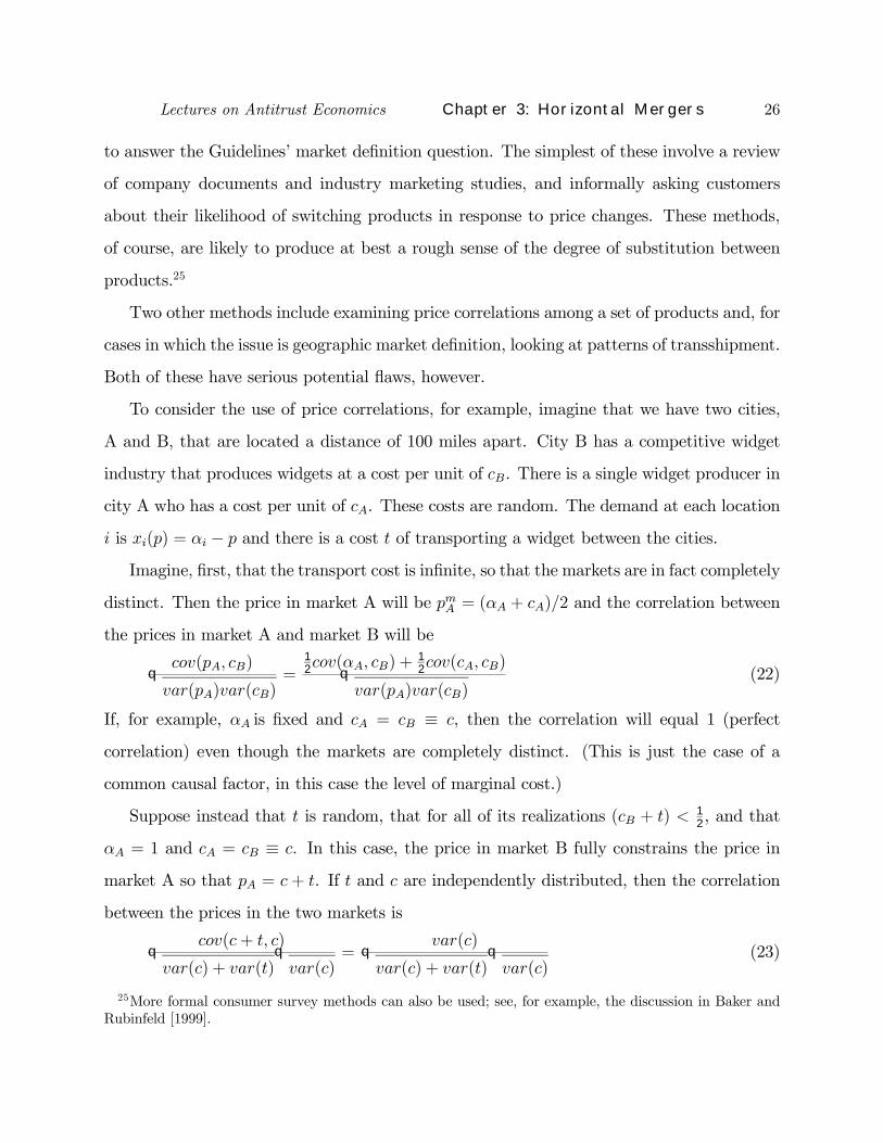
products.25
Two other methods include examining price correlations among a set of products and, for
cases in which the issue is geographic market deÞnition, looking at patterns of transshipment.
Both of these have serious potential ßaws, however.
To consider the use of price correlations, for example, imagine that we have two cities,
A and B, that are located a distance of 100 miles apart. City B has a competitive widget
industry that produces widgets at a cost per unit of cB. There is a single widget producer in
city A who has a cost per unit of cA. These costs are random. The demand at each location
i is xi(p) = αi − p and there is a cost t of transporting a widget between the cities.Imagine, Þrst, that the transport cost is inÞnite, so that the markets are in fact completely
distinct. Then the price in market A will be pmA = (αA + cA)/2 and the correlation between
the prices in market A and market B will be
cov(pA, cB)qvar(pA)var(cB)
=12cov(αA, cB) +
12cov(cA, cB)q
var(pA)var(cB)(22)
If, for example, αA is Þxed and cA = cB ≡ c, then the correlation will equal 1 (perfect
correlation) even though the markets are completely distinct. (This is just the case of a
common causal factor, in this case the level of marginal cost.)
Suppose instead that t is random, that for all of its realizations (cB + t) < 12, and that
αA = 1 and cA = cB ≡ c. In this case, the price in market B fully constrains the price in
market A so that pA = c + t. If t and c are independently distributed, then the correlation
between the prices in the two markets is
cov(c+ t, c)qvar(c) + var(t)
qvar(c)
=var(c)q
var(c) + var(t)qvar(c)
(23)
25More formal consumer survey methods can also be used; see, for example, the discussion in Baker andRubinfeld [1999].

Lectures on Antitrust Economics Chapter 3: Horizontal Mergers 27
Hence, if var(c) is small, the correlation between the prices will be nearly zero, despite the
fact that market A is fully constrained by the competitive industry in market B. On the
other hand, if the variance of t is instead small, then the correlation will be close to 1. Yet
� and this illustrates the problem � which of var(c) or var(t) is small has no bearing on
the underlying competitive situation.
A problem with looking at transshipments is also illustrated by this last case since no
transshipments take place in equilibrium despite the fact that market A is fully constrained
by market B.
4.2 Evidence on the Effects of Increasing Concentration on Prices
In the consideration of �other factors�, one type of evidence that is often presented by one
or both sides in horizontal merger cases is evidence of the effects of concentration on prices.
These studies typically follow the �Structure-Conduct-Performance� paradigm of regressing
a measure of performance � in this case price � on one or more measures of concentration
and other control variables.26 A typical regression seeking to explain the price in a cross-
section of markets i = 1, ..., I might look like
pi = β0 + wi · β1 + yi · β2 + CRi · β3 + εi, (24)
where wi are variables affecting costs, yi are variables affecting demand, and CRi are mea-
sures of the level of concentration (the variables might be in logs, and both linear and
nonlinear terms might be included). In the most standard treatment, these variables are all
treated as exogenous causal determinants of prices in a market. As such, and given the mix
of demand and cost variables included in the regression, it has become common to refer to
them as �reduced form� estimations (see, for example, Baker and Rubinfeld [1999]), with
the intention of distinguishing them from �structural estimation� of demand and supply
relationships.
26The use of price in structure-conduct-performance studies was most forcefully advocated by Weiss [1990].

Lectures on Antitrust Economics Chapter 3: Horizontal Mergers 28
Regressions such as these have seen wide application in horizontal merger cases; indeed,
they are the most commonly used econometric technique employed in current merger cases.
In the Federal Trade Commission�s challenge of the Staples/Office Depot merger, for example,
this type of regression was used by both the Commission and the defendants.27 In that merger
the focus was on whether these office �superstores� should be considered as a distinct market
(or �submarket�) or whether these stores should be viewed as a small part of a much larger
office supply market. The parties used this type of regression to examine the determinants of
Staples� prices in a city.28 In that case, the concentration measures included both a measure
of general concentration in the office supply market and measures of whether there were
office supply superstores within the same Metropolitan Statistical Areas and within given
radiuses of the particular Staples store.
As another example, when the Union PaciÞc (UP) sought to acquire the Southern PaciÞc
(SP) railroad in 1996 shortly after the merger of the Burlington Northern (BN) and the
Sante Fe (SF) railroads, many railroad routes west of the Mississippi River would go from
being served by 3 Þrms to being served by 2 Þrms in the event of the merger, and some would
go from 2 Þrms to 1 Þrm. The merging parties claimed that SP was a �weak� railroad, and
that it did not have much of a competitive effect on UP in any market in which BN/SF was
already present. To bolster this claim, the merging parties conducted this type of study of
UP�s prices, where the concentration variables included separate dummy variables indicating
exactly which competitors UP faced in a particular market.29
Although these regressions have provided useful evidence in a wide range of cases, they
can suffer from at least two serious problems. The Þrst has to do with omitted variables.
Omitted variables is of course a potential problem in any regression analysis, but it bears
special mention here. Firms typically have many �assets� that affect their competitive po-
27For an interesting discussion of the use of econometric evidence in the case, see Baker [1999b].28The data was actually a panel of stores over time, rather than just a single cross-section or time series
as in equation (24).29The case was presented before the Surface Transportation Board, which has jurisdiction over railroad
mergers.

Lectures on Antitrust Economics Chapter 3: Horizontal Mergers 29
sition in a market and it is unusual for an analyst to have measures of all of the important
ones, or even most. As a result, the included measure(s) of concentration can end up cap-
turing the effects of these omitted factors. One might hope that this would not matter;
perhaps the concentration variable(s) can serve as a useful aggregate proxy for these factors?
Unfortunately, it seems like this will often not be the case. To take an example, consider
the UP/SP example. One factor that is probably important for the determination of prices
on a route is the level of aggregate capacity available on that route (such as tracks, sidings,
and yards); higher capacity is likely to lead to lower prices, all else equal. In the pre-merger
data, this aggregate capacity level is likely to be correlated with the number and identity
of competitors on a route. For example, aggregate capacity is probably larger when more
Þrms are present. Hence, in a regression that includes the number of Þrms on a route, but
not capacity, some of the effect that is attributed to an increase in concentration is likely
to be due instead to the fact that across the population of markets, higher concentration
is correlated with lower capacity levels. But in a merger, while the number of Þrms will
decrease on many routes, the level of capacity on these routes may well remain unchanged
(at least in the short-run). If so, the regression would predict too large an elevation in price
following the merger.
The second problem has to do with endogeneity of some of the explanatory variables. In
fact, (24) is not a true reduced form, since the level of concentration is surely endogenous.30
A true reduced form would include only the underlying exogeneous factors inßuencing market
outcomes. Indeed, in many ways equation (24) is closer to estimation of a supply relation,
in the sense discussed in Bresnahan [1989]. To see this, consider the case in which demand
takes the constant elasticity form X(p) = Ap−η, all Þrms are identical with constant unit
costs of c, and Þrms play a static Cournot equilibrium. Then we can write an active Þrm�s
30Often some of the other right hand side variables are as well. For example, in studies of airline pricing,it is common to include the load factor on a route � the share of available seats that are sold � as aright-hand side variable affecting costs.

Lectures on Antitrust Economics Chapter 3: Horizontal Mergers 30
Þrst-order condition as
p = c− P 0(X)xi = c+ siηp = c +
H
ηp (25)
where P (·) is the inverse demand function and si is Þrm i�s market share which, given
symmetry, equals the HerÞndahl index H. As in Bresnahan [1989], we can nest this model
and perfect competition by introducing a conduct parameter θ and rewriting (25) as
p = c+ θH
ηp.
Thus,
p =
Ãη
η − θH!c, (26)
where the term in parentheses represents the proportional �mark-up� of price over marginal
cost. Taking logarithms, we can write (26) as
ln(p) = ln(c) + ln(η)− ln(η − θH). (27)
Supposing that marginal cost takes the form c = ceε where c is observable (or a function of
observable variables) and ε is an unobservable cost component, (27) becomes
ln(p) = ln(c) + ln(η)− ln(η − θH) + ε, (28)
which has a form very close to (24) (the only difference is the interaction between the
concentration variable H and the demand variable η). In fact, using the Þrst-order Taylor
expansion that ln(x) ≈ x− 1, we can approximate (28) by
p = c+ θH + ε, (29)
which takes exactly the linear form often used in these studies. Here H is endogeneous;
possible instruments for it include the �market size� variable A, and measures of the cost of
entry, both of which affect the level of concentration while arguably being uncorrelated with
ε. For more general demand and cost structures, or cases with asymmetric Þrms, the true
supply relation will not take a form so close to (24), but (24) might be viewed as a loose

Lectures on Antitrust Economics Chapter 3: Horizontal Mergers 31
approximation to the supply relation. The sense in which it is a �reduced form� approach is
then really only that those who run such regressions do not attempt to relate their estimates
back to any underlying structural model.
5 Breaking the Market DeÞnition Mold
In this section, I discuss three techniques for evaluating the likely effects of a merger on
competition that do not follow the approach suggested in the Guidelines. These are merger
simulation, residual demand estimation, and the event study approach.
5.1 Merger Simulation
If we are really going the route of estimating demand and cost functions to answer the
Guidelines� questions, one might wonder why we don�t just examine the price effects of the
merger directly using these estimated structural parameters. That is, once we estimate a
structural model of the industry using pre-merger data, we can simulate the effects of the
merger. Conceptually, doing so is simple: given demand and cost functions for the various
products in the market and an assumption about the behavior of the Þrms (existing studies
typically examine a static simultaneous price choice game), one can solve numerically for the
equilibrium prices that will emerge from the post-merger market structure. For example, if
Þrms 1 and 2 in a three-Þrm industry merge, the equilibrium prices (p∗1, p∗2, p
∗3) in a static
simultaneous price choice game will be such that after the merger (p∗1, p∗2) maximizes the
merged Þrm�s proÞt given p∗3 (the notation follows that in Section 4.1),
(p∗1, p∗2) = argmaxp1,p2
Xi=1,2
[pixi(p1, p2, p∗3, q, y)− ci(xi(p1, p2, p
∗3, q, y))],
while p∗3 maximizes the proÞt of the third Þrm given (p∗1, p∗2),
p∗3 = argmaxp3p3x3(p
∗1, p
∗2, p3, q, y)− c3(x2(p
∗1, p
∗2, p3, q, y)).
Given explicit functional forms for the demand and cost functions, Þxed point algorithms (or,
in some cases, explicit solutions using linear algebra), can be used to Þnd the post-merger

Lectures on Antitrust Economics Chapter 3: Horizontal Mergers 32
equilibrium prices. (More detailed discussions of the method can be found in Hausman,
Leonard, and Zona [1994], Nevo [2000b], and Werden and Froeb [1994].) With the recent
advances in estimating structural models, this approach is gaining increasing attention.
There are, however, two important caveats regarding this method. First, a critical part
of the simulation exercise involves the choice of the post-merger behavioral model of the
industry. An obvious response is to try to estimate this behavior using pre-merger data,
a technique that has a long history in the empirical industrial organization literature (see,
for example, Bresnahan [1987, 1989] and Porter [1983]).31 One serious concern, however, is
that the Þrms� behavior may change as a result of the merger. For example, the reduction
in the number of Þrms could cause an industry to go from a static equilibrium outcome
(say, Bertrand or Cournot) to a more cooperative tacitly collusive regime. In principal, this
too may be something that we can estimate if we have a sample of markets with varying
structural characteristics. But, to date, those attempting to conduct merger simulations
have not done so.
Second, it is important to recall that pricing is likely to be only one of several important
variables that may be affected by a merger. Entry, long-run investments in capacity, and
R&D are among the variables that may be signiÞcantly affected by a merger. Indeed, welfare
� whether consumer welfare or aggregate welfare � may in the long-run be more affected
by these other variables than by pricing. Unfortunately, as we noted earlier, the empirical
industrial organization literature is really only at the very beginning of getting a handle on
these important issues.
In recent work, Peters [2003] evaluates the perfomance of these simulation methods by
examining how well they would have predicted the actual price changes that followed six
airline mergers in the 1980s. The standard merger simulation technique, in which price
changes arise from changes in ownership structure (given an estimated demand structure and
inferred marginal costs) produces the price changes shown in the column labeled �Ownership
31Alternatively, one could simply compare the actual premerger prices with those predicted under variousbehavioral assumptions, as in Nevo [2000b].

Lectures on Antitrust Economics Chapter 3: Horizontal Mergers 33
Change� in Table 3.1.32 The actual changes, in contrast, are in the last column, labeled
�Actual %∆p in the table. While the merger simulation captures an important element of
the price change, it is clear that it predicts the price changes resulting from the various
mergers imperfectly. For example, the US Air-Piedmont merger (US-PI) is predicted to
lead to a smaller price increase than either the NW-RC or TW-OZ mergers, but the reverse
actually happened.
Table 3.1: Simulated and Actual Price Changes From Airline Mergers (Peters [2003])
Peters next asks how much of this discrepency can be accounted for by other observed
changes that occurred following the merger, such as changes in ßight frequency or entry,
by including these changes in the post-merger simulation. The column labeled �Observed
Changes� in Table 3.1 reports the answer. As can be seen there, these observed changes
account for little of the difference.33
Given this negative answer, Peters then looks to see whether changes in unobserved prod-
uct attributes (such as Þrm reputation or quality, denoted by µ in the table) or in marginal
costs (denoted by c in the table) can explain the difference. The changes in unobserved
product attributes can be inferred using the pre-merger estimated demand coefficients by
solving for the levels of these unobserved attributes that reconcile the post-merger quantities
purchased with the post-merger prices. Given the inferred post-merger unobserved product
32See Peters [2003] for a discussion of how different assumption about the demand structure affect theseconclusions.33It should be noted, however, that Peters looks only at the year following consummation of the merger.
These changes may be more signiÞcant over a longer period.

Lectures on Antitrust Economics Chapter 3: Horizontal Mergers 34
attributes, Peters can solve for the Nash equilibrium prices that would obtain were product
attributes to have changed in this way, assuming that marginal costs remained unchanged.
(Observe that since the post-merger attributes are obtained entirely from the demand side,
these computed equilibrium prices need not equal the actual observed prices.) As can be
seen in the column labeled �Change in µ,� this accounts for little of the difference between
predicted and actual prices.
Finally, Peters can infer a change in marginal cost, by calculating the levels of marginal
costs that would make the computed Nash equilibrium prices equal to the actual post-merger
prices. (This is done by including all of the previous changes, including the inferred changes
in unobserved product attributes µ, and solving for marginal costs from the Nash equilibrium
pricing Þrst-order conditions, as discussed earlier in the chapter.) The price change reported
in the column labeled �Change in c� reports the size of the price change if these marginal
cost changes are included in the simulation, omitting the product attribute changes. As
can be seen in the table, the changes due to changes in c represent a large portion of the
discrepency between the initial simulation and the actual price changes.
It should be noted, however (as Peters does), that an alternative interpretation of these
results is that it was Þrm conduct rather than marginal costs that changed post-merger. For
example, this seems most clear in the case of the CO-PE merger, where the acquired airline
was suffering serious Þnancial difficulty prior to the merger. In this case, prices undoubtedly
increased not because of a true marginal cost change, but rather because of a change in the
previously distressed Þrm�s behavior. Changes in behavior may have occurred in the other
mergers as well. At the very least, however, Peters� study suggests directions that are likely
to be fruitful in improving prospective analyses of mergers.
It seems clear that as our techniques for estimating structural models get better, merger
simulation will become an increasingly important tool in the analysis of mergers. How quickly
this happens, however, and the degree to which it supplants other techniques, remains to be
seen.

Lectures on Antitrust Economics Chapter 3: Horizontal Mergers 35
5.2 Residual Demand Estimation
Another technique that does not follow the Guidelines� path, but that also avoids a full-
blown structural estimation, is the residual demand function approach developed by Baker
and Bresnahan [1985]. SpeciÞcally, Baker and Bresnahan propose a way to determine the
increase in market power from a merger that involves separately estimating neither the
cross-price elasticities of demand between the merging Þrms� and rivals� products nor rivals�
behavioral reactions. As Baker and Bresnahan put it:
...evaluating the effect of a merger between two Þrms with n− 2 other competi-tors would seem to require the estimation of at least n2 parameters (all of the
price elasticities of demand), a formidable task....That extremely difficult task
is unnecessary, however. The necessary information is contained in the slopes
of the two single-Þrm (residual) demand curves before the merger, and the ex-
tent to which the merged Þrm will face a steeper demand curve.... The key to
the procedures is that the effects of all other Þrms in the industry are summed
together. ...This reduces the dimensionality of the problem to manageable size;
rather than an n-Þrm demand system, we estimate a two-Þrm residual demand
system. [p.59]
To understand the Baker and Bresnahan idea, it helps to start by thinking about the
residual demand function faced by a single Þrm (i.e., its demand curve taking into account
rivals� reactions), as in Baker and Bresnahan [1988]. SpeciÞcally, consider an industry with
N single-product Þrms and suppose that the inverse demand function for Þrm 1 is given by
p1 = P1(x1, x−1, z), (30)
where x1 is Þrm 1�s output level, x−1 is an (N − 1)-vector of output levels for Þrm 1�s rivals,and z are demand shifters. To derive the residual inverse demand function facing Þrm 1,
Baker and Bresnahan posit that the equilibrium relation between the vector x−1 and x1 given

Lectures on Antitrust Economics Chapter 3: Horizontal Mergers 36
the demand variables z and the cost variables w−1 affecting Þrms 2, ..., N can be denoted by
x−1 = B−1(x1, z, w−1). (31)
For example, imagine for simplicity that there are two Þrms in the industry (N = 2). If
equilibrium output levels are determined by either a static simultaneous-choice quantity
game or by a Stackleberg game in which Þrm 1 is the leader, then (31) is simply Þrm 2�s
best-response function. Substituting for x−1 in (30) we can then write Þrm 1�s residual
inverse demand function as
p1 = P1(x1, B−1(x1, z, w−1), z) ≡ R1(x1, z, w−1). (32)
For example, in the simple case in which z and w−1 are both scalar variables, we might
estimate this in the simple constant elasticity form:
ln(p1i) = γ0 + γ1 ln(x1i) + γ2 ln(zi) + γ3 ln(w−1,i) + εi. (33)
Baker and Bresnahan would then look to the estimate of γ1, the quantity elasticity of the
residual inverse demand function, as a measure of the Þrm�s market power.34
Note that since x1 will typically be correlated with ε, we will require an instrument for
x1. Moreover, since the rivals� cost variables w−1 are already in the estimating equation (33),
this will need to be a cost variable that affects only Þrm 1, say w1. Figure 3.3 depicts the
idea of what identiÞes the residual demand function R1(·). Imagine that Þrms other thanÞrm 1 produce a homogeneous product, that Þrm 1�s product is differentiated, and that the
N Þrms compete by simultaneously choosing quantities. By holding the demand variable z
and the cost variables w−1 for Þrm 1�s rivals Þxed, the estimating equation (33) effectively
holds the aggregate best-response function of the rivals Þxed, which is labeled as B−1(·)in Figure 3.3.35 A shift in the cost variable for Þrm 1 from w1 to w01 < w1 shifts Þrm 1�s
best-response function outward as depicted in Figure 3.3. This increases x1 and reduces the
34A similar derivation to that above can be done to derive instead a residual ordinary (rather than inverse)demand function.35That is, the function B−1(·) is the sum of the quantities in the vector function B−1(·).
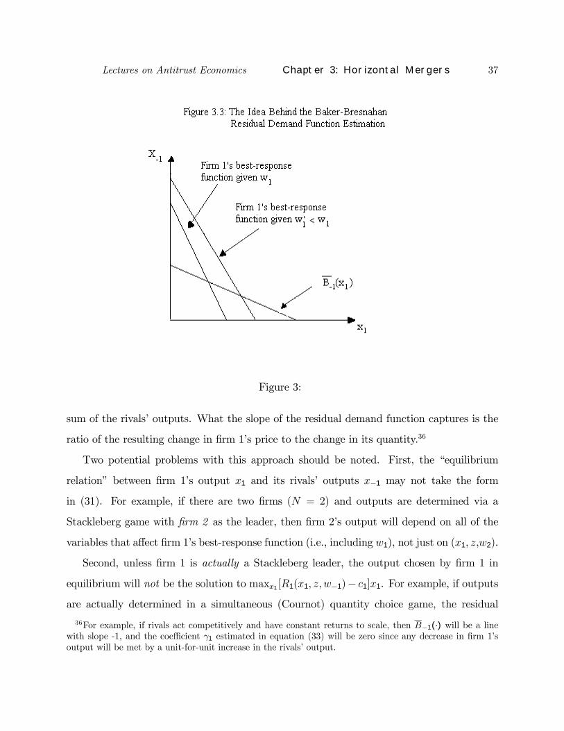
Lectures on Antitrust Economics Chapter 3: Horizontal Mergers 37
Figure 3:
sum of the rivals� outputs. What the slope of the residual demand function captures is the
ratio of the resulting change in Þrm 1�s price to the change in its quantity.36
Two potential problems with this approach should be noted. First, the �equilibrium
relation� between Þrm 1�s output x1 and its rivals� outputs x−1 may not take the form
in (31). For example, if there are two Þrms (N = 2) and outputs are determined via a
Stackleberg game with Þrm 2 as the leader, then Þrm 2�s output will depend on all of the
variables that affect Þrm 1�s best-response function (i.e., including w1), not just on (x1, z,w2).
Second, unless Þrm 1 is actually a Stackleberg leader, the output chosen by Þrm 1 in
equilibrium will not be the solution to maxx1[R1(x1, z, w−1)− c1]x1. For example, if outputs
are actually determined in a simultaneous (Cournot) quantity choice game, the residual
36For example, if rivals act competitively and have constant returns to scale, then B−1(·) will be a linewith slope -1, and the coefficient γ1 estimated in equation (33) will be zero since any decrease in Þrm 1�soutput will be met by a unit-for-unit increase in the rivals� output.

Lectures on Antitrust Economics Chapter 3: Horizontal Mergers 38
demand function derived from this procedure will not have any direct correspondence to the
actual price-cost margins in the market.
Baker and Bresnahan�s procedure for evaluating a merger expands on this idea. Imagine,
for simplicity, an industry in which initially there are three Þrms and suppose that Þrms 1
and 2 will merge, and that Þrm 3 will remain independent (the idea extends to any number
of independent Þrms as above). Now suppose that the inverse demand functions for Þrms 1
and 2 are
p1 = P1(x1, x2, x3, z) (34)
and
p2 = P2(x1, x2, x3, z). (35)
As before, suppose that Þrm 3�s best-response function is
x3 = B3(x1, x2, z, w3). (36)
Substituting as before we can write:
p1 = R1(x1, x2, z, w3) (37)
p2 = R2(x1, x2, z, w3). (38)
Equations (37) and (38) give the residual inverse demands faced by the merged Þrms 1
and 2 taking into account Þrm 3�s reactions to their price choices. Given estimates of these
equations, Baker and Bresnahan propose evaluating the merger by computing the percentage
price increase caused for each of the merging Þrms by a 1% reduction in both of their outputs,
and comparing this to the two merging Þrms� single-Þrm residual inverse demand elasticities
(as derived above); if these elasticities are much greater in the former case, they conclude
that the merger increases market power.
Unfortunately, this method for evaluating post-merger market power suffers from the
same two problems as in the single Þrm case. Moreover, a new problem emerges with the

Lectures on Antitrust Economics Chapter 3: Horizontal Mergers 39
method Baker and Bresnahan use to compare pre- and post-merger market power: since
both of the merging Þrms could not have been Stackleberg leaders prior to the merger, the
single Þrm residual inverse demand elasticities are clearly not directly related to pre-merger
mark-ups.37
5.3 The Event Study Approach
Our third non-Guidelines empirical technique for examining the effect of a merger aims to
do so without any kind of structural estimation. The simple idea, originally due to Eckbo
[1983] and Stillman [1983], is as follows: A merger that will raise the prices charged by the
merging Þrms is good for rivals, while one that will lower these prices is bad for them. Hence,
we should be able to distinguish these two cases by looking at rivals� stock price reactions
to the merger announcement and any subsequent enforcement actions. (Eckbo and Stillman
looked at these reactions for a number of mergers and found no positive effects on rivals,
and therefore concluded that most mergers are not anticompetitive.)
Although a very simple technique (it uses the very standard event study method), it has
a number of potential pitfalls. The Þrst has to do with the power of the test. McAfee and
Williams [1988], for example, examined what they argue was an �obviously anticompetitive
merger� and found no evidence of statistically signiÞcant positive stock price reactions by
rivals. They argue that the problem is that the rivals may be large Þrms with highly variable
stock returns so that the power of test may be low; i.e., we shouldn�t take observing no
statistically signiÞcant reaction in rivals� stock prices to mean that the merger will not raise
prices.
Another issue has to do with what the literature calls �precedent effects.� If a merger
is announced, this may convey information about market (or regulatory) conditions more
generally. For example, consider the announcement of an efficiency-enhancing merger. This
37In the special case in which the merged Þrm will act as a Stackleberg leader, we can however use theestimates of (37) and (38) to derive the post-merger prices by solving maxx1,x2
Pi=1,2[Ri(x1, x2, z, w3)−ci]xi
for the merged Þrm�s optimal quantities (x∗1, x∗2) and then computing p∗1 = R1(x∗1, x∗2, z, w3) and p∗2 =R2(x∗1, x∗2, z, w3).

Lectures on Antitrust Economics Chapter 3: Horizontal Mergers 40
announcement may indicate not only that the merged Þrms� costs will fall, but also that
the other Þrms in the industry are likely to follow their example by merging themselves.
Typically, the resulting reduction in all Þrms� costs will lead to both lower prices and higher
proÞts. Thus, the informational content of this announcement � what it says about likely fu-
ture mergers and their effects � will lead rivals� stock prices to increase upon announcement
of this price-reducing merger.38
In the other direction, there is a possibility that a merger that increases the size of a Þrm
could also increase the likelihood of anticompetitive exclusionary behavior. For example,
in a �deep pocket� model of predation in which the size of a Þrm�s asset holdings affects
its ability to predate on rivals (e.g., Benoit [1984], Bolton and Scharfstein [1990]), a merger
might increase the likelihood that rivals are predated upon. This could lead to negative
returns for rival stock values from announcement of a price-increasing merger.
These interpretational difficulties can be substantially avoided by looking instead at cus-
tomer stock prices as is done by Mullins, Mullins, and Mullins [1995]. Doing so allows one
to look directly at the stock market�s expectation of the changes in price (as well as any
non-price dimensions of net surplus such as quality) that will be produced by the merger.
Mullins, Mullins, and Mullins study the United States Steel (USS) dissolution suit that was
Þled in 1911. They begin by identifying 13 potentially signiÞcant events in the history of the
case, and then narrow their focus down to Þve events by restricting attention to those events
which caused a statistically signiÞcant movement in USS�s stock price. The Þve events are
described in Table 3.2, which also indicates with a (+) or a (-) whether the event is associated
with an increase or a decrease in the probability of dissolution.
38In principal, we can try to distinguish between anticompetitive and precedent effects by looking fordifferential stock price responses among rivals: competitive effects should be felt more strongly by rivals thatcompete more closely with the merging Þrms. In this way, Prager [1992] Þnds evidence of precedent effectsin her study of the 1901 merger between Great Northern Railway and the Northern PaciÞc Railway. Onecaveat, however, is that the precedent effect may in some cases also be more relevant for these same Þrms.

Lectures on Antitrust Economics Chapter 3: Horizontal Mergers 41
Table 3.2: Mullins, Mullins, and Mullins [1995] Event Descriptions
They then examine the effects of these events on the stock market values of four sets
of Þrms: steel industry rivals, railroads, the Great Northern Railway, and street railway
companies. Examining steel industry rivals follows the Eckbo-Stillman method.39 Railroads
and street rail companies, in contrast, were both customers of USS, in that they bought
signiÞcant quantities of steel.40 The event responses for these groups to the Þve events are
shown in Table 3.3, which also shows the response of USS to each event.41 As can be seen
in the table, the responses of steel industry rivals are generally insigniÞcant. The railroad
stocks, however, respond in a statistically and economically signiÞcant way to these events,
and in a direction that suggests that dissolution of USS would lower steel prices. Indeed,
since steel represented only 10% of railroad costs, the 2% value reduction that railroads felt
in response to the USRUMOR event would correspond to a 20% reduction in the expected
cost of steel if the probability of the merger went from 0 to 1 as a result of this news, and
even more otherwise.39The set of steel rivals excludes the Great Northern Railway which had a complicated relationship with
USS due to USS�s lease of the Great Northern Railway�s iron ore holdings. Mullins, Mullins, and Mullinsexamine the effects of the events on the Great Northern Railway separately, which I do not report here.40The railroads were both customers and suppliers to USS, since a great deal of steel was shipped by rail.
Mullins, Mullins, and Mullins argue that the effects on both suppliers and customers should be similar inthis case because there is evidence that no secret rebates were granted off of the existing regulated rail rates,and so the effect of the merger on both suppliers and customers should be a function only of the change inthe output of steel.41Street rail stock prices were available only toward the end of the sample period.

Lectures on Antitrust Economics Chapter 3: Horizontal Mergers 42
Table 3.3: Average Estimated Event Responses in Mullins, Mullins, and Mullins [1995]
While Mullins, Mullins, and Mullins found signiÞcant effects on customers, it should be
noted that Þnding no statistically signiÞcant customer stock price response to a merger�s
announcement may not indicate the absence of a price effect: If customers are themselves
producers, any price increases may be fully passed on to Þnal consumers. In addition, as
noted in the McAfee-Williams critique, the power of such a test may be low.
Of course, this entire method assumes that stock market participants have an accurate
forecast of the competitive effects of the merger. Moreover, in the typical merger investi-
gation, the antitrust agencies would be able to ask directly the opinions of a wide range of
industry and stock market participants, and so the additional information gained by this
method may not be that great.
6 Examining the Results of Actual Mergers
All of the foregoing discussion has focused on a prospective analysis of horizontal mergers.
It is natural to ask, however, what we know, looking retrospectively, about their actual
effects. Such analyses can be useful for at least two reasons. First, they can guide our priors
about the likelihood of mergers being anticompetitive or efficiency-enhancing (ideally, as a

Lectures on Antitrust Economics Chapter 3: Horizontal Mergers 43
function of their characteristics). Second, we can use this information to assess how well
various methods of prospective merger analysis perform, as in the Peters [2003] paper that
we discussed in Section 5.1.
Unfortunately, the economics literature contains remarkably little of this kind of analysis.
In the remainder of the chapter, I discuss the few studies that have looked at either price
or efficiency effects in actual mergers (none look at both). This is clearly an area where we
could use more research.42
6.1 Price Effects
A small number of studies have analyzed the effects of actual mergers on prices. Many of
these have focused on the airline industry, where a number of high-proÞle mergers occurred
in the mid-1980s and price data is publicly available because of data reporting regulations.
Borenstein [1990] studies the effects of the mergers of Northwest Airlines (NW) with Republic
Airlines (RC) and Trans World Airlines (TW) with Ozark Airlines (OZ) in 1985/1986. In
both cases, the merging airlines had their major hub at the same airport: Minneapolis served
as the hub for both NWand RC; St. Louis was the hub for TWand OZ.43 Both mergers began
in 1985 with Þnal agreements reached in the Þrst quarter of 1986, and received regulatory
approval (from the Department of Transportation) in the third quarter of 1986. Table 3.4
shows the average prices before and after the mergers for four categories of markets, deÞned
by whether both merging Þrms operated before the merger and by whether they faced any
competition before the merger (�other Þrms�). The �relative prices� columns record for the
third quarters of 1985, 1986, and 1987 the average over markets in the respective category
of the percentage difference between the average price for the merging Þrms in that market
and the average price for a set of markets of a similar distance. The �average change� over
42To the extent that this limited amount of work is due to a lack of data, one way to enhance our knowledge(or at least that of the DOJ and FTC) may be for the enforcement agencies to require parties to approved(or partially approved) mergers to provide the agencies with information for some period of time after theirmerger.43NW and RC accounted for 42% and 37% respectively of enplanements at Minneapolis; TW and OZ
accounted for 57% and 25% of enplanements at St Louis.

Lectures on Antitrust Economics Chapter 3: Horizontal Mergers 44
1985-87 is the average over markets in the respective category of the percentage difference
between the 1987 �relative price� in the market and the 1985 �relative price.�44
Table 3.4: Merging Airlines� Price Changes at Their Primary Hubs (Borenstein [1990])
The results in Table 3.3 reveal very different experiences following the two mergers. Prices
increased following the NW/RC merger, but not following the TW/OZ merger. Looking at
the different categories in the NW/RCmerger, (relative) prices increased by 22.5% on average
in markets which were NW and RC duopolies prior to the merger.45 It is also noteworthy
that prices increased as well on routes in which NW and RC did not compete prior to the
44Note that this average price change is therefore not equal to the change in the average relative pricesreported in the relative price columns.45Peters [2003], however, reports somewhat different price changes for these same mergers. In his data,
prices increased 7.2 percent and 16.0 in the NW/RC and TW/OZ mergers, respectively, in markets that wereinitally served by both merging Þrms. (Across the six mergers Peters studies, prices increased between 6 and30 percent in such markets.) Peters reports that they increased 11.0 percent and 19.5 percent, respectively, inmarkets where these Þrms faced no pre-merger competition. The reason for the differences from Borenstein�sresults is unclear.
Lectures on Antitrust Economics Chapter 3: Horizontal Mergers 45
merger. This could reßect a price-constraining effect of potential entry prior to the merger,
increased market power arising from domination of the hub airport after the merger, or
in the case of markets in which they faced competitors, the effects of increased levels of
multimarket contact with competitor airlines. Borenstein also notes that the prices of other
airlines on these routes dislayed a pattern very similar to the pattern seen for the merging
Þrms in Table 3.4.
Kim and Singal [1993] expand on Borenstein�s analysis by examining the price changes
resulting from 14 airline mergers that occurred from 1985 to 1988. Table 3.5 depicts the
average of the changes in the relative prices for routes served by the merging Þrms compared
to all other routes of similar distance. The table is divided horizontally into three sections:
The Þrst �full period� section looks at the change in prices from one quarter before the Þrst
bid of the acquirer to one quarter after consummation of the merger; the second �announce-
ment period� section looks at changes from one quarter before the Þrst bid of the acquirer
to one quarter after this bid; the third �completion period� section looks at changes from
one quarter before consummation to one quarter after. The table is also divided into two
sections vertically. The left section looks at the merging Þrms� price changes, while the right
section looks at rivals� price changes on the routes served by the merging Þrms. Within each
of these sections, price changes are computed separately depending upon whether one of the
merging Þrms was Þnancially distressed prior to the merger.

Lectures on Antitrust Economics Chapter 3: Horizontal Mergers 46
Table 3.5: Changes in Relative Fares of Merging and Rival Firms (Kim and Singal [1993])
Looking at price changes for the merging Þrms, we see that relative prices rose by an
average of 3.25% over the full sample period in mergers involving Þrms that were not Þnan-
cially distressed. They rose substantially more (26.25%) in mergers involving a Þnancially
distressed Þrm. The announcement period and completion period changes are interesting as
well. One might expect market power effects to be felt prior to the actual merger (as the
management teams spend time together), while merger-related efficiencies would occur only
after completion. For mergers involving �normal Þrms� we indeed see that prices rise in the
announcement period, and fall � although not as much � in the completion period.46 (The46It is perhaps a little surprising, however, that substantial efficiencies would be realized so soon after
completion. Moreover, there is some evidence (Kole and Lehn [2000]) that these mergers may have led to

Lectures on Antitrust Economics Chapter 3: Horizontal Mergers 47
patterns for mergers involving a failing Þrm are more puzzling.) Price changes for rival Þrms
again follow very similar patterns. Kim and Singal also examine through regression analysis
the relationship between the change in relative fares and the change in the HerÞndahl Index.
Consistent with the efficiency interpretation just given, they Þnd that for mergers involving
�normal Þrms�, the size of the price elevation during the announcement period is highly
correlated with the change in concentration induced by the merger, while the fall in prices
during the completion period is unrelated to this change.
Finally, Kim and Singal break the merging Þrms� routes into four categories depending
upon whether the route involves a common hub airport for the merging Þrms (if so, it is a
�Hub� route) and whether the merging Þrms both served the route prior to the merger (if
so, it is an �overlap� market). Table 3.6 depicts their results for the full period. Notably for
mergers involving normal Þrms, prices fall on �Hub only� routes and they have no change
on Hub/Overlap routes. (Moreover, Singal and Kim show that these price reductions come
entirely during the completion period.) These changes strongly suggest the presence of
merger-related efficiency beneÞts. �Overlap Only� markets show a price change like that
seen in Table 3.5 for the full sample. Finally, note that routes that are neither a hub route
nor an overlap route also experience price increases that are of this magnitude. These may
reveal the effect of increased multimarket contact.47
increases rather than decreases in marginal costs.47Evans and Kessides [1994] perform a �structure-conduct-performance�-style study of the relation between
airline prices and both concentration and multimarket contact during this period and Þnd positive andeconoically signiÞcant price effects from both factors. Their Þndings also provide indirect evidence on theeffects of the airline mergers during this period, because most of the changes in concentration and multimarketcontact in their sample were attributable to mergers.

Lectures on Antitrust Economics Chapter 3: Horizontal Mergers 48
Table 3.6: Relative Fare Changes for Four Categories of Routes (Kim and Singal [1993])
Peters [2003], which was largely focused on evaluating merger simulation techniques (see
Section 5.1), documents as well the service changes and entry events that followed six of
these mergers. Peters shows that ßight frequency tended to decrease in markets that were
initially served by both merging Þrms, and increase in markets that were initially served by
only one of the merging Þrms. The mergers also led to entry, although these changes in the
number of rivals were only statistically signiÞcant for three of the mergers.
Banking is another industry in which Þrms are required to provide the government with
data on their operations. Prager and Hannan [1998] study the price effects of mergers in
the banking industry for the period January 1992 through June 1994. They examine the
change in deposit rates for three types of deposits, NOW accounts (interest bearing check-
ing accounts), MMDA accounts (personal money market deposit accounts48), and 3MOCD
accounts (three-month certiÞcates of deposit). Hannan and Prager separately examine the
effects of �substantial horizontal mergers� for which the HerÞndahl Index in the effected
48These have restricted check-writing privileges.

Lectures on Antitrust Economics Chapter 3: Horizontal Mergers 49
market increases by at least 200 points to a post-merger value of at least 1800, and �less
substantial mergers�, for which the HerÞndahl increases by at least 100 points to a post
merger value of at least 1400 and which were not �substantial mergers�. Their price data
are monthly observations on deposit interest rates from October 1991 through August 1994,
while their estimating equation takes the form
ratchgit = α +TXt=2
δtIt ++12Xn=−12
βnSMint ++12Xn=−12
γnLSMint + εit,
where ratchgit = ln(rateit/ratei,t−1) and rateit is bank i0s deposit rate in period t, It is a
dummy variable taking value 1 in period t and 0 otherwise, SMint is a dummy variable taking
value 1 if bank i was exposed to a substantial horizontal merger in period t+n, and LSMint
is a dummy variable taking value 1 if bank i was exposed to a less substantial horizontal
merger in period t+n. 49 The results from this estimation can be seen in Table 3.7, where the
merger exposure effects are presented in three aggregates: the premerger period (n = −12to n = 0), the post merger period (n = 1 to n = +12), and the total period.
49In fact, matters are somewhat more complicated than this, because the pricing data are at the banklevel, not the market (SMSA) level. Hence, the merger exposure variables are actually weighted averages(by deposits) of the exposures that a given bank i has in the various markets in which it operates.

Lectures on Antitrust Economics Chapter 3: Horizontal Mergers 50
Table 3.7: Price Effects of �Substantial� and �Less than Substantial� Bank Mergers
(Prager and Hannan [1998])
The results indicate that substantial mergers reduce the rates that banks in a market offer.
This effect is largest for NOW accounts (approximately a 17% reduction in rates), for which
customers arguably have the strongest attachment to local banks, and least for three-month
CD�s (less than 2% reduction in rates, and not statistically signiÞcant). Notably, however,
Prager and Hannan Þnd that less substantial mergers increase rates paid in the market. One
possible interpretation of this difference is that these mergers involve efficiencies (which allow
banks, absent other effects, to increase their rates), but the effects of these efficiencies on
prices are more than offset by an increase in market power for substantial mergers. Finally,
although the results in Table 3.7 do not distinguish between the price changes for merging
Þrms and their rivals, Prager and Hannan Þnd that these two groups had very similar price

Lectures on Antitrust Economics Chapter 3: Horizontal Mergers 51
effects, paralleling the Borenstein and Kim and Singal Þndings on this point.50
6.2 Efficiencies
Just as with price effects, remarkably little has been done examining the effects of horizontal
mergers on productive efficiency, at least given the issue�s importance. Most of the work
examining the efficiency effects of mergers has examined mergers in general, rather than
focusing on horizontal mergers. In general, the effects need not be the same. On the one
hand, there may be greater potential for synergies when the merging Þrms are in the same
industry; on the other hand, since horizontal mergers may increase market power, even
efficiency decreasing horizontal mergers may be proÞtable for merging Þrms.51
Work examining mergers in general has generally found that there is a great deal of
heterogeneity in merger outcomes. Some mergers turn out well, others very badly.52 As well,
the average effects are sensitive both to the time period examined and the particular sample
of mergers studied. Perhaps the best known study of post-merger performance is Ravenscraft
and Scherer [1987], who document using the FTC�s Line of Business data (collected for just
three years from 1974-76) a dramatic decline in post-merger proÞtablity of acquired lines
of business, which generally were highly successful prior to acquisition. Ravenscraft and
Scherer�s sample, however, consisted largely of acquisitions from the conglomerate merger
wave of the 1960s. Two different studies have examined data from the years following this
conglomerate merger wave, Lichtenberg and Siegel [1987] and McGuckin and Nguyen [1995].
Lichtenberg and Siegel examine the effect of ownership changes on statistically estimated
plant-level total factor productivity using the Census Bureau�s Longitudinal Establishment
50In one other study, Barton and Sherman [1984] document the price changes that occurred following the1976 and 1979 acquisitions of two competitors by a manufacturer of two types of duplicating microÞlm. Theyprovide evidence consistent with price increases following the merger. The data they use comes as a resultof a 1981 FTC antitrust suit seeking to reverse the acquisitions.51One reason for greater synergies may simply be that the managers of the acquiring Þrm are more likely
to understand the business of the acquired Þrm; see, for example, Kaplan, Mitchell, and Wruck [2000].52This is also consistent with the event study analysis of stock price returns, which Þnds wide variation
in how the market evaluates announced mergers. At the same time, as the case studies in Kaplan [2000]document, a merger�s performance may end up very different from the market�s inital forecast.

Lectures on Antitrust Economics Chapter 3: Horizontal Mergers 52
Data (LED) Þle for the years 1972 to 1981. (Total factor productivity is determined in
much of their work as the residual from estimation of a Cobb-Douglas production function.)
As can be seen in Table 3.8, in contrast to the Ravenscraft and Scherer Þndings, they Þnd
that acquired plants were less productive than industry averages prior to acquisition, but
had productivity increases that brought them almost up to the industry average afterwards.
This may reßect the un-doing of Ravenscraft and Scherer�s inefficient conglomerate mergers.
Table 3.8: Differences in Mean Levels of Productivity between Plants Changing Ownership
in Year t and Plants Not Changing Ownership (Lichtenberg and Siegel [1987])
The LED database, however, contains primarily large plants. McGuckin and Nguyen
[1995] study the same question using instead the Census Bureau�s Longitudinal Research
Database (LRD) for the years 1977-1987. They restrict attention to mergers occurring
between 1977-1982 and focus on the food manufacturing industry (SIC 20). This sample
includes many more small plants than in Lichtenberg and Siegel�s analysis. It also includes
plants that operated during only part of the sample period (an �unbalanced panel�), while
Lictenberg and Siegel used a balanced panel (a balanced panel may worsen selection biases).
However, most of their analysis uses labor productivity (the average product of labor relative

Lectures on Antitrust Economics Chapter 3: Horizontal Mergers 53
to the industry average product) instead of a measure of total factor productivity. In contrast
to Lichtenberg and Siegel, they Þnd that acquired plants tend on average to have above-
average productivity prior to acquisition, although they Þnd that this is not true when
they restrict attention to large plants like those studied by Lichtenberg and Siegel. Like
Lichtenberg and Siegel, they Þnd post-merger productivity improvements.
Unfortunately, neither of these studies deals with endogeneity or selection issues when
estimating productivity, which we know (see, Olley and Pakes [1996]) can seriously bias
productivity estimates. Moreover, the latter study, as we have noted, bases its Þndings on
labor productivity, rather than total factor productivity, which can reßect shifts in input
mixes. In addition, neither of these studies considers separately the effects of horizontal
mergers. In fact, we would ideally like to know how horizontal mergers affect productivity
conditional on their structural attributes (e.g., potential for increasing market power), since
these attributes affect which mergers managers pursue.53
One study that examines horizontal mergers explicitly is Pesendorfer [1998], who studies
a horizontal merger wave in the paper industry in the mid 1980s. Rather than estimating
productivity directly, Pesendorfer tries to infer pre and post-merger productivity using the
Þrms� capacity choices. (Much as we discussed in Sections 4.1 and 5.1, he infers marginal costs
from the Cournot-like Þrst-order conditions for capacity choice.) This is an interesting idea,
but is not entirely convincing in this application for several reasons. First, the investment
Þrst-order conditions he uses are entirely static, while investment choices are likely to be
affected by dynamic considerations. Second, the procedure relies on an assumed investment
cost function (this might not be necessary if one uses a panel). Finally, one cannot distinguish
whether the changes in marginal cost he derives reßect shifts of the plant�s marginal cost
function or movements along an unchanging function.
Recent work, most notably Olley and Pakes [1996] (see also Levinsohn and Petrin [2003]),
53Another thing that affects the mergers that managers pursue is the antitrust policy in effect at any giventime. Thus, using information on efficiency effects (or price effects, for that matter) to determine apprpriateantitrust policy must recognize this endogeneity.

Lectures on Antitrust Economics Chapter 3: Horizontal Mergers 54
has greatly improved our abilities in estimating productivity. The examination of the pro-
ductivity effects of horizontal mergers seems a natural and highly valuable direction for this
work to go.
References
Andrade, G., M. Mitchell, and E. Stafford [2001], �New Evidence and Perspectives onMergers,� Journal of Economic Perspectives (15), 103-20.
Baker, J.B. [1999a], �Developments in Antitrust Economics,� Journal of EconomicPerspectives (13), 181-94.
Baker, J.B. [1999b], �Econometric Analysis in FTC v. Staples,� Journal of PublicPolicy & Marketing (18), 11-21.
Baker, J.B. and D.L. Rubinfeld [1999], �Empirical Methods Used in Antitrust Litiga-tion: Review and Critique,� American Law and Economics Review (1), 386-435.
Baker, J.B. and T.F. Bresnahan [1985], �The Gains to Merger or Collusion in Product-Differentiated Industries, Journal of Industrial Economics (33), 427-44.
Baker, J.B. and T.F. Bresnahan [1988], �Estimating the Residual Demand Curve Fac-ing a Single Firm,� International Journal of Industrial Organization (6), 283-300.
Barton, D.M. and R. Sherman [1984], �The Price and ProÞt Effects of HorizontalMerger: A Case Study,� Journal of Industrial Economics (33), 165-77.
Benoit, J.-P. [1984], �Financially Constrained Entry in a Game with Incomplete Infor-mation,� RAND Journal of Economics (4), 490-9.
Berry, S.T. [1994], �Estimating Discrete Choice Models of Product Differentiation,�RAND Journal of Economics (25), 242-62.
Berry, S. and A. Pakes [1993], �Some Applications and Limitations of Recent Advancesin Empirical Industrial Organization: Merger Analysis,� American Economic ReviewPapers and Proceedings (83), 247-52.
Berry, S. and A. Pakes [1993], �Some Applications and Limitations of Recent Advancesin Empirical Industrial Organization: Merger Analysis,� American Economic Review(83), 247-52.
Berry, S., J. Levinsohn, and A. Pakes [1995], �Automobile Prices in Market Equilib-rium,� Econometrica (63), 841-90.

Lectures on Antitrust Economics Chapter 3: Horizontal Mergers 55
Bolton, P. and D. Scharfstein [1990], �A Theory of Predation Based on Agency Prob-lems in Financial Contracting,� American Economic Review (80), 93-106.
Borenstein, S. [1990], �Airline Mergers, Airport Dominance, and Market Power,�American Economic Review (80), 400-4.
Bresnahan, T.F. [1987], �Competition and Collusion in the American Automobile In-dustry: The 1955 Price War,� Journal of Industrial Economics (35), 457-82.
Bresnahan, T.F. [1989], �Empirical Methods in Industries with Market Power,� in R.Schmalensee and R. Willig, eds., Handbook of Industrial Organization (Volume II),Amsterdam: Elsevier.
Brock, W. and J. Scheinkman [1985], �Price-Setting Supergames with Capacity Con-straints,� Review of Economic Studies (52), 371-82.
Carlton, D. and R. Gertner [1989], �Market Power and Mergers in Durable GoodsIndustries,� Journal of Law and Economics (32), S203-26.
Coase, R.H. [1972], �Durability and Monopoly,� Journal of Law and Economics (15),143-49.
Compte, O., F. Jenny, and P. Rey [2002], �Capacity Constraints, Mergers, and Collu-sion,� European Economic Review (46), 1-29.
Eckbo, B.E. [1983], �Horizontal Mergers, Collusion, and Stockholder Wealth,� Journalof Financial Economics (11), 241-73.
Evans, W.N. and I.N. Kessides [1994], �Living by the �Golden Rule�: MultimarketContact in the U.S. Airline Industry,� Quarterly Journal of Economics (109), 341-66.
Farrell, J. and C. Shapiro [1990], �Horizontal Mergers: An Equilibrium Analysis,�American Economic Review (80), 107-26.
Gowrisankaran, G. [1999], �A Dynamic Model of Endogenous Horizontal Mergers,�RAND Journal of Economics (30), 56-83.
Hausman, J.A. [1996], �Valuation of New Goods Under Perfect and Imperfect Compe-tition,� in T. Bresnahan and R. Gordon, eds., The Economics of New Goods, Studiesin Income and Wealth (58), Chicago: National Bureau of Economic Research.
Hausman, J., G. Leonard, and J.D. Zona [1994], �Competitive Analysis with Differen-tiated Products,� Annales D�Economie et de Statistique (34), 159-80.
Jensen, M.C. and R.S. Ruback [1983], �The Market for Corporate Control: The Sci-entiÞc Evidence,� Journal of Financial Economics (11), 5-50.

Lectures on Antitrust Economics Chapter 3: Horizontal Mergers 56
Kaplan, S.N., ed. [2000], Mergers and Productivity, Chicago: University of ChicagoPress.
Kaplan, S.N., M.L. Mitchell, and K.H. Wruck [2000], �A Clinical Exploration of ValueCreation and Destruction in Acquisitions: Organizational Design, Incentives, and In-ternal Capital Markets,� in S.N. Kaplan, ed., Mergers and Productivity, Chicago: Uni-versity of Chicago Press.
Kole, S. and K. Lehn [2000], �Workforce Intgration and the Dissipation of Value inMergers: The Case of USAir�s Acquisition of Piedmont Aviation,� in S.N. Kaplan, ed.,Mergers and Productivity, Chicago: University of Chicago Press.
Kim, E.H. and V. Singal [1993], �Mergers andMarket Power: Evidence from the AirlineIndustry,� American Economic Review (83), 549-69.
Levinsohn, J. and A. Petrin [2003], �Estimating Production Functions Using Interme-diate Inputs to Control for Unobservables,� Review of Economic Studies (70), 317-41.
Lichtenberg, F.R. and D. Siegel [1987], �Productivity and Changes in Ownership ofManufacturing Plants,� Brooking Papers on Economic Activity: Special Issue on Mi-croeconomics, Washington, D.C.: The Brookings Institution.
Mankiw, N.G. and M.D. Whinston [1986], �Free Entry and Social Inefficiency,� RANDJournal of Economics (17), 48-58.
Mas-Colell, A., M.D. Whinston, and J.R. Green [1995], Microeconomic Theory, NewYork: Oxford University Press.
McAfee, R.P. and M.A. Williams [1988], �Can Event Studies Detect AnticompetitiveMergers?,� Economics Letters (28), 199-203.
McAfee, R.P. and M.A. Williams [1992], �Horizontal Mergers and Antitrust Policy,�Journal of Industrial Economics (40), 181-6.
McGuckin, R.H. and S.V. Nguyen [1995], �On Productivity and Plant OwnershipChange: New Evidence from the Longitudinal Research Database,� RAND Journal ofEconomics (26), 257-76.
Mullin, G.L., J.C. Mullin, and W.P. Mullin [1995], �The Competitive Effects of merg-ers: Stock Market Evidence from the U.S. Steel Dissolution Suit,� RAND Journal ofEconomics (26), 314-30.
Nevo, A. [1997], Demand for Ready-to-Eat Cereal and Its Implications for Price Com-petition, Merger Analysis, and Valuation of New Goods, Harvard University Ph.D.Dissertation.

Lectures on Antitrust Economics Chapter 3: Horizontal Mergers 57
Nevo, A. [2000a], �A Practitioner�s Guide to Estimation of Random Coefficients LogitModels of Demand,� Journal of Economics and Management Strategy (9), 513-48.
Nevo, A. [2000b], �Mergers with Differentiated Products: The Case of the Ready-to-Eat Cereal Industry,� RAND Journal of Economics (31), 395-421.
Nevo, A. [2001], �Measuring Market Power in the Ready-to-Eat Cereal Industry,�Econometrica (69), 307-42.
Olley, G.S. and A. Pakes [1996], �The Dynamics of Productivity in the Telecommuni-cations Equipment Industry,� Econometrica (64), 1263-98.
Perry, M.K. and R. Porter [1985], �Oligopoly and the Incentive for Horizontal Merger,�American Economic Review (75), 219-27.
Pesendorfer, M. [1998], �Horizontal Mergers in the Paper Industry,� NBER WorkingPaper No. 6751.
Peters, C. [2003], �Evaluating the Performance of Merger Simulation: Evidence fromthe U.S. Airline Industry,� Northwestern University, Center for the Study of IndustrialOrganization Working Paper # 32.
Porter, R.H. [1983], �A Study of Cartel Stability: The Joint Executive Committee,1880-1886,� Bell Journal of Economics (14), 301-14.
Prager, R.A. [1992], �The Effects of Horizontal Mergers on Competition: The Case ofthe Northern Securities Company,� RAND Journal of Economics (23), 123-33.
Prager, R.A. and T.H. Hannan [1998], �Do Substantial Horizontal Mergers GenerateSigniÞcant Price Effects? Evidence from the Banking Industry,� Journal of IndustrialEconomics (46), 433-52.
Ravenscraft, D.J. and F.M. Scherer [1987],Mergers, Sell-offs, and Economic Efficiency,Washington, D.C.: Brookings Institution.
Salant, S., S. Switzer, and R. Reynolds [1983], �Losses from Horizontal Mergers: TheEfect of an Exogenous Change in Industry Structure on Cournot-Equilibrium,� Quar-terly Journal of Economics (98), 185-99.
Shleifer, A. and L.H. Summers [1988], Breach of Trust in Hostile Takeovers,� in A.Auerbach, ed., Corporate Takeovers: Causes and Consequences, Chicago: Universityof Chicago Press, 33-56.
Stillman, R. [1983], �Examining Antitrust Policy Towards Horizontal Mergers,� Jour-nal of Financial Economics (11), 225-40.
Weiss, L.W., ed. [1990], Concentration and Price, Cambridge, MA: MIT Press.

Lectures on Antitrust Economics Chapter 3: Horizontal Mergers 58
Werden, G. [1990], �Antitrust Policy Toward Horizontal Mergers: A Comment on Far-rell and Shapiro,� Department of Justice Economic Analysis Group Discussion PaperNo. 90-4.
Werden, G. and L. Froeb [1998], �The Entry-Inducing Effects of Horizontal Mergers:An Exploratory Analysis,� Journal of Industrial Economics (46), 525-43.
Werden, G. and L. Froeb [1994], �The Effects of Mergers in Differnetiated ProductsIndustries: Logit Demand and Merger Policy,� Journal of Law, Economics, and Orga-nization (10), 407-26.
Williamson, O.E. [1968], �Economies as an Antitrust Defense: The Wefare Tradeoffs,�American Economic Review (58), 407-26.