lectures in micro meteorology - dtu...

General rights Copyright and moral rights for the publications made accessible in the public portal are retained by the authors and/or other copyright owners and it is a condition of accessing publications that users recognise and abide by the legal requirements associated with these rights.

• Users may download and print one copy of any publication from the public portal for the purpose of private study or research. • You may not further distribute the material or use it for any profit-making activity or commercial gain • You may freely distribute the URL identifying the publication in the public portal

If you believe that this document breaches copyright please contact us providing details, and we will remove access to the work immediately and investigate your claim.

Downloaded from orbit.dtu.dk on: Jun 12, 2018

Lectures in Micro Meteorology

Larsen, Søren Ejling

Publication date:2015

Document VersionPublisher's PDF, also known as Version of record

Link back to DTU Orbit

Citation (APA):Larsen, S. E. (2015). Lectures in Micro Meteorology. DTU Wind Energy. (DTU Wind Energy E; No. 0075).

http://orbit.dtu.dk/en/publications/lectures-in-micro-meteorology(58cf5d7c-de82-44ac-a827-74ac4075f9b5).html


Søren E Larsen

02 2015

Lectures in MIcro Meteorology Report DTU-Windenergy-E-0075 2015 By Søren E Larsen Copyright: Reproduction of this publication in whole or in part must include the customary

bibliographic citation, including author attribution, report title, etc. Cover photo: [Text] Published by: Department of Wind Energy, Frederiksborgvej 399 Request report from:

www.dtu.dk

ISSN: [0000-0000] (electronic version) ISBN:

978-87-93278-18-9 (electronic version)

ISSN: [0000-0000] (printed version) ISBN: [000-00-0000-000-0] (printed version)

Preface

This report contains the notes from my lectures on Micro scale meteorology at the Geophysics Department of the Niels Bohr Institute of Copenhagen University. In the period 1993-2012, I was responsible for this course at the University. At the start of the course, I decided that the text books available in meteorology at that time did not include enough of the special flavor of micro meteorology that characterized the work of the meteorology group at Risø (presently of the Institute of wind energy of the Danish Technical University). This work was focused on Boundary layer flows and turbulence and was often aimed at applications like wind energy, wind loads, dispersion and deposition, air-sea exchange and air-land exchange, as well as flow response to surface inhomogeneity. The course, dimensioned to 60 hours, was generally structured in the first year, based on copies of papers and copies of the overheads used for presentation. But it gradually filled out in the following years, as with power points and the typed manuscripts constituting this reports. Most writing was finalized within the first 10 years of the course, meaning most references are somewhat dated by now, although I have not resisted adding more recent work, if ongoing projects made it easy. In the course I have tried to present the details of the basic material, trying to avoid the well known sentence of “It is easily seen—“. But I have been less thorough and pedagogical, when presenting the more illustrative material. The original report includes pages of course material, directly copied from other people’s publications, used during the lectures. Therefore this report is an internal report only. In the present report these copied pages have been removed in respect for the rights of the original authors. DTU-Wind Energy, 02 2015 Søren Ejling Larsen


Content

Summary ....................................................................................................................................... 5

1. Introduction .......................................................................................................................... 6

2. Concepts, scales of motion and statistical tools ................................................................. 7

3. Basic equations ................................................................................................................. 41

4. Mean flow, turbulence and closures. ................................................................................. 60

5. The Ekman boundary layers ............................................................................................. 80

6. The atmospheric surface boundary layer. Monin-Obuchov scaling ................................ 94

7. Near surface viscous layers, roughness lengths: z0 and z0T, interfacial exchange. ....... 118

8. Scaling in the atmospheric boundary layer. .................................................................... 142

9. Horizontally heterogeneous boundary layers. ................................................................. 165

10. Dispersion plumes from chimneys. ................................................................................. 207

11. Boundary layer climate, radiation, surface energy balance. ........................................... 220

12. Wind climate, wind energy, wind loads ........................................................................... 232

13. Instruments, measurements and data............................................................................. 244

References ................................................................................................................................ 268

Acknowledgements ................................................................................................................... 278


Summary

The report contains the authors lecture notes to courses in micro scale meteorology and atmospheric turbulence. The course has aimed to touch upon both the basic theories and the special formulation aiming at application. The structure of the course can be seen from the “Content”. It has a chapter on concepts and statistics, two chapters on the basic fluid dynamics and turbulence closure. Three chapters on various atmospheric scaling laws, Ekman layer, surface layer and total boundary layer. It includes one chapter on the roughness and the surface–atmosphere exchange, one chapter on heterogeneous boundary layers, and one on atmospheric diffusion and turbulence. It has two chapters on boundary layer climatology involving radiation, temperature and wind issues, and finally a chapter discussing measurement and instrumental problems. The report has been loosely edited compared to the original notes. [Text - The following line contains a section break - do not delete]

Lectures in Micro Meteorology 5

1. Introduction

Characteristics of the atmospheric planetary boundary layer (ABL) , also called the planetary boundary layer (PBL), are of direct importance for much human activity and well being, because humans basically live within the PBL. Hence, we basically derive our wind energy from winds in the PBL, and most of our air pollution is dispersed, deposited and chemically transformed within the PBL. The importance stems as well from atmospheric energy and water cycles issues, because the fluxes of momentum, heat, and water vapour between the atmosphere and the surfaces of the earth all pass through the PBL, being carried and modified by mixing processes here. Since these mixing processes mostly owe their efficiency to the mechanisms of boundary layer turbulence, a proper quantitative description of the turbulence processes becomes essential for a satisfying description of the fluxes between the surface and the atmosphere. Description of the structure of the flow, relevant scalar fields, turbulence and flux through the atmospheric boundary layers necessitates that almost all types of the flows, that occur there, must be considered. For these objectives, there are very few combinations of characteristic boundary layer conditions that are not of significant importance, at least for some parts of the globe.

6 Lectures in Micro Meteorology

2. Concepts, scales of motion and statistical tools

Additionally to the synoptic weather patterns, the meteorology of the PBL is strongly influenced by the surface characteristics and turbulence structure. Therefore, we will in this introductory section shortly summarise qualitative aspects the different processes influencing the PBL conditions additionally to a more detailed discussion of the statistical methods used in general and which we shall use throughout the text to describe the characteristics of the PBL. Both with respect to mean characteristics, variability and fluxes the PBL is dominated by turbulent motion. Therefore it is appropriate firstly to consider what we should understand with turbulence, a subject that has filled many pages in the scientific literature. Here we just notice that motions of systems that can be described by the nonlinear fluid equations tend to show strongly varying stochastic components, the turbulence, as well as more smooth and predictable characteristics. Turbulence can occur on many scales of motion and be described by as either two-dimensional motion or three-dimensional motion. In the PBL, the wind speed as well as temperature and humidity, and indeed all atmospheric variables, show this stochastic behaviour on all spatial and temporal scales of variation. In figures 2.1, this is illustrated by a measured time series of the wind speed observed through different time windows. The following figures 2.2-26 all illustrate different processes and scales of variability within the PBL. While the motion in the PBL can vary on virtually all scales, the processes within the PBL that create so called PBL turbulence occur most on time scales of the order of and less than one hour, with associated spatial scales. This PBL turbulence is three dimensional and therefore can carry most of the vertical fluxes that is essential for the coupling between the atmosphere and the surface. On these time scales the main mechanism for producing turbulence is the vertical gradient of the mean wind. In figure 2.2 we show typical vertical variations of wind speed, humidity, and temperature between their surface values and values at the top and above the PBL. Temperature and humidity can both increase and decrease with height, depending on whether their surface values or values in the free atmosphere are the larger. However, the wind speed will always increase with height from zero at the ground to its value in the free atmosphere just above the PBL. The vertical wind shear gives rise to overturning of the air, producing the turbulence (Tennekes and Lumley, 1982). This provides a formidable mechanism for carrying the vertical fluxes compared to the molecular transport mechanism that would have been an alternative. For example, a temperature gradient of 2 K across the lowest 10 meter height with a wind speed at 5 m/s give rise to a heat flux of about 0.5 mK/s (or 600 W/m2). If the flux had to be carried by molecular diffusion only, the result would be 4·10-6 mK/s (or 5 mW/m2) only. The temperature structure of the PBL strongly influences the turbulence production through its influence on the density of the air. If the air is warmer and thereby lighter close to the ground, it will enhance the production; if it is cooler at the ground the production will be reduced. To a lesser extent the humidity has similar, although smaller effect because also admixture of water vapour changes the density of the air.


Figure. 2.1 Upper figure: Wind speed measured 30 meter above flat homogeneous terrain in Denmark from Troen and Petersen (1989). The data were obtained from a one-year time series recorded with 16-Hz resolution. Each graph shows the measured wind speed over the time period indicated. The number of data points in each graph is 1200; each averaged over 1/1200 of the time period indicated. The vertical axis is wind speed, 0-20 meter/sec. Lower figure: Similar plot from Jensen and Busch (1982) here based on 1000 points per plot. The lack of fine structure in the 10 sec plot is due to the onset of viscous dissipation at the highest frequencies here, see discussion of spectra in the end of this section.


Figure 2.2. Characteristic height variations (profiles) of the mean values of the wind speed,u temperature,T and humidity, q from the ground

to the top of the PBL, indicated by h. Also shown by the arrows on the u-profile is the overturning of the flow induced by the vertical velocity gradient. The profiles are shown for the following characteristic situations:

a) Thermally unstable, e.g. a sunny day. b) thermally stable, e.g. a clear sky night,

and c) Thermally neutral, e.g. a high-wind

overcast situation. The size and magnitude of the turbulent eddies are indicted by the rotational motion indicated on the figure. Instead of temperature, T, one will in meteorology typically use the potential temperature, θ, see section 3.(larsen,1993) Based on the above discussion we can now specify the planetary boundary layer as being the layer through which the atmospheric variables change between their values in the free atmosphere and their values at the surface, the transition being mostly controlled by turbulent motion and mixing. The structure and character of the turbulence will be different for the different thermal conditions, as is shown below in figure 2.3, illustrating the turbulence structure for thermally unstable and stable conditions. Figure 2.3 Depiction of the turbulence structure for unstable and stable atmospheric boundary

layers. From Wyngaard (1990)


Above we have discussed the PBL as it was horizontally homogenous, meaning that only the vertical variation was important. Next we shall illustrate the horizontal structure of a PBL as in figure 2.4 and its diurnal variation in figure 2.5.

Figure 2.4 Horizontalvariability in a PBL. The PBL is seen as constituted by a number of overlapping and interacting “internal boundary layers”, reflecting the different surface characteristics. We shall later discuss this in detail.

The different characteristics of the PBL, depicted above, all operate at different timescales and spatial scales. The diurnal cycle is of obvious importance for the chance of regimes seen in

figures 2.2 and 2.5. The height of the PBL and the terrain features are seen to impose different length scales in figures 2.3 and 2.4, and overall will the time and spatial scales of the synoptic

flow be seen in the PBL.

Figure 2.5. Diurnal variation of a PBL, from Stull (1991). The figure depicts the rise of the PBL height with surface heating at sun rise, and the subsequent rise of the night time PBL after sun set by radiational cooling. Obviously overcast conditions will modify this turn of event, see figure 2.2. In figures 2.2 and 2.3 the production of turbulence is envisioned as a swirling motion induced by the shear, and modified by the temperature structure. A whorl constitutes a volume of localized vorticity, which we shall denote an “eddy”. This picture of turbulence, as a soup of


intertwining spaghetti-like eddies, has been very useful in the study of turbulence in spite of its extreme simplicity. Each eddy can be associated with a size, or spatial scale, and a time or timescale. When eddies have been produced they will remain coherent for some time, creating their own smaller scale shear. By the same process as for the mean shear this eddy shear will create smaller eddies transferring the kinetic energy to smaller and smaller eddies, until it is turned into heat by the viscocity of the air. Similarly many other atmospheric processes can be characterised by their time and spatial scales, describing roughly the time they typically takes and their extent when they occur. In Fig. 2.6 is depicted a number of characteristic processes and their characteristic spatial and temporal scales, ranging from weather systems, with a timescales of about one week and a spatial scale of about 1000 km, and down to the smallest turbulence eddies, called dissipation range, where the fluid eddies have such small scales that they are disrupted by viscosity and the kinetic energy is turned into heat. The characteristic scales here are about five ms and five millimetres. Fig. 2.6 is in a way a space-time scale representation of the atmospheric motions that are presented as time signals in Fig. 2.1.

Figure 2.6. Time and space scales for the processes influencing the flow in the atmospheric boundary layer (Busch et al., 1979). The three motion categories of smallest scale, all belong to the category of three dimensional atmospheric turbulence that are of key importance for the structure of the atmospheric boundary layer, and will be described more in the text. For comparison are shown as well characteristic spatial scales for aspects of the wind power technology


From Figure 2.6 reflects that there seems to be a rough relation between the spatial and the time scales of the different motion elements, meaning that large scale motion elements are associated with large time scales and smaller scales motions are associated smaller time scales. From the figure is seen that there is proportionality between the time scales and the spatial scales of a motion type corresponding to about 1 m/s For the three dimensional atmospheric PBL turbulence, the above rough proportionality is formulated more precisely by Taylor’s hypothesis of frozen turbulence, which state that the turbulence field does change very little, whiles it is blowing past the observer by the mean speed. Hence, what is observed as a time change over the time τ corresponds in reality to a spatial change along the direction of the mean flow of the length ℓ, such that:

(2.0) ℓ = U ∙ τ,

where U is the mean speed.

This simple formulation works remarkably well, and means that for this type of turbulence one is really measuring the spatial variation (along the mean wind direction) by measuring the time variation from a stationary meteorology mast. In view of the above discussion we shall next consider a few of the statistical tools used to describe the atmospheric boundary layer turbulence. The coordinate system: We have two vectors in the system, the position, r[m], and the velocity U(m/s) (2.1) 1 2 3 1 2 3 = (x , x , x ) = ( x, y, z ). = (u , u , u ) = ( u, v, w).Ur

Here the numbered variables are usual when formulating the governing equations in tensor form. The other variables are often used when the equations are written in their component forms. We have as well a number of scalar variables: The independent variable time: t (sec). Temperature: T [K]. The air density: ρ [kg/m3]. Water vapour: ρw [kg/m3], water vapour mixing

ration: q = ρw /ρ. Concentrations of admixture: C [kg/m3], mixing ratio for C: c = C/ρ.

We shall consider an atmospheric variable. It can be any of those we have defined, U, T, q, C, c. For generality, we use the variables s and e. We consider the variables as stochastic Both variables can be any of the variables above s, e, u1, u2, u3, T, q, C, c. The variables s, e are functions of space and time: s = s (xi, t), where i refers to the three coordinate numbers: 1, 2, 3. The simplest statistical operator is the average or the mean value. We typically operate with three types of averages: Ensemble averages, time averages and spatial averages. Averages are typically denoted by an over-bar, or a bracket, like <s>, or by capital letters.

Figure 2.7. Commonly used coordinate systems and variables, with a practical example for near surface turbulent velocity and temperature. Notice that the average vertical and lateral velocity are both close to zero, but smaller scale velocity turbulence is three dimensional. W is close to zero, because vertical mean values and slow fluctuations cannot exist close to the ground. V is close to zero, because the horizontal coordinate system is aligned with the x along the mean wind. The Ensemble Average: We imagine that our variable, s = s (xi, t), is part of an ensemble of representations of the variable, s. Hence we write: sj = sj (xi , t), where j is the ensemble index.

(2.2)1

( , ) ( , )N

i j iEj

s x t s x tN

= ∑

Ensemble average is easiest to imagine for the case of a wind tunnel simulation, where one can restart the tunnels over and over again, and this way obtain an ensemble. For an atmospheric boundary layer one may imagine that the boundary layer is started over and over with similar start conditions and similar boundary conditions.

The coordinate system

x3 z is always vertical!!

x3

z

u3

w

x2 y

u 2v

x1 x

u1 u

T, C, q

t


The use of ensemble averages is most convenient when doing mathematics, e.g. taking the average of model output, where each output can be considered one ensemble. Also, it is the average we use when averaging equations to yield equations for the average variables. In practice one will often use time or space averages, either because the signals available are functions of these parameters as e.g. for measurements of time series from meteorological towers, or because of the objectives of the study, as for example area averages often being the goal of hydrological studies. The averaging procedures employed are limited by the signals available but are also a matter of choice. As an example, we can take the signal in figure 2.1 that would lend itself to time averaging, since it is a time signal, but also to ensemble averaging using ensembles of data from similar days or hours. Time average: Here, we average our variable, s = s (xi, t), over a given time interval 2T to obtain:

(2.3)1

( , ) ( , )2

T

i iT

T

s x t s x t dT

τ τ−

= +∫

Time averages are especially convenient in connection with time series-obviously. Also all measurements are associated with time (and space!) averaging, because of the finite time and space resolution of all physical instruments. An example of a practical time averaging procedure is shown on figure 2.8 below. Figure 2.8. Time series of wind speed and the formation of the time average.

Spatial averages: Here, we average over a spatial interval ∆. This interval can be a volume, an area and a line average.

(2.4)1

( , ) ( , ) ,2

i i i ins x t s x t dχ χ

∆

∆

− ∆

= +∆∫ .

where the power n reflects the dimensionality of the integral, n=1, 2, or 3. Spatial averages are much used when working with numerical models, where one kind of average is the average across a grid-element. From measurements, an area average is typical what a satellite sees, since it averages over the footprint. A line average would be what can be detected from airplane measurements and also from some kind of LIDAR or RADAR scattering instrumentation.


Ergode theorem: Assume that s (xi, t) is statistically stationary and homogeneous, and then we have

(2.5) lim ( , ) lim ( , ) lim ( , ) .i i iT NT Ns x t s x t s x t s const

∆→∞ ∆→∞ →∞= = = = .

For such conditions we can therefore in the limit change between the different average values, since they are all the same, but only when we can consider the variables statistically stationary and homogeneous and when the series are long enough in both time and the relevant space dimensions. Statistically stationary means that all statistics of s is independent of t. Statistically homogeneous means similarly that all statistics of s is independent of xi. Note s (xi, t) can be homogeneous in some of the dimensions, xi, and not in others. For example in the boundary layer we have learned that the wind speed increases with height. Therefore in general wind speed is not homogeneous in the vertical but it can well be considered so along the horizontal axes, see figure 2.2.

Whenever, we use ( , )is x t without indications of which kind of averaging that is applied, it

should either be obvious from the context or it will mean ensemble average. Fluctuations. For a stochastic variable, s, we define the fluctuation as the difference between the s and its mean value. The fluctuation is typically indicated by s′ . (2.6) s s s′ = −

Funny enough this very simple equation is honoured with a name: The Reynolds Convention. The mean value of the fluctuation is zero:

(2.7) ( ) 0s s s s s′ = − = − = .

Since s is a constant and the average of a constant is the same constant. Frequency distributions, pdf’s, (Co-) Variances, standard deviations, STD. Variances and standard deviations are measures of the magnitude of the fluctuations. The variance of fluctuations is found by averaging the square of the fluctuation:

(2.8) 2 20 ss s s σ′ ′ ′< = = , where σs is the so-called standard deviation. Alternatively one can determine the variance as:

(2.9) 2 2 2.( )( )s s s s s s s′ = − − = − . The covariance is found from two signals, s and e, as follows.

(2.10) ( ) ( ) .s e s s e e′ ′ = − −

The magnitude of the covariance depends on two features, the magnitude of the two fluctuations, s´ and e´, and how well they correlate with each other. To separate these two features one often study the normalise co-variance, called the correlation. It is defined by:

Figure 2.9. The same time series as in figure 2.8, but here with the computation of an estimate of the variance. Also shown is the frequency distribution of the fluctuations, s’, used to describe the frequency of amplitudes of the fluctuations around the mean value with the variance.. The covariance is found from two signals, s and e, as follows.

(2.11) ( ) ( ) .s e s s e e′ ′ = − − The magnitude of the covariance depends on two features, the magnitude of the two fluctuations, s´ and e´, and how well they correlate with each other. To separate these two features one often study the normalise co-variance, called the correlation. It is defined by:

(2.12) 1 1ese s

e sρσ σ′ ′

− ≤ = ≤ ,

where the bounds on esρ corresponds to the two situations that s and e are either in perfect

correlation or in perfect counter-correlation, that is s’ = e’ or s’ = -e’. Notice, 2 2/ 1ss σ′ = .

Commutation rules for Ensemble averaging and mathematical operations: Recall that the ensemble average, as defined in (2.3), is just a sum:

(2.13)1

1 N

jj

s u for NN =

≡ → ∞∑ ,

This means summation and differencing commutes with averaging! Differentiation and averaging:


(2.14)1 1

1 1;

N Nj

jj j

dede d dee

dx N dx dx N dx= =

= = =∑ ∑

Similarly for integration:

(2.15) .i isdx dt sdx dt=∫ ∫

However, multiplication and averaging do not commute:

(2.16) ( )( ) ,e s e e s s e s es se s e e s s e s e′ ′ ′ ′ ′ ′ ′ ′⋅ = + + = ⋅ + + + = ⋅ + ≠ ⋅ since the correlation in general is different from zero. Covariances involving a velocity component can be interpreted a transport along the direction of the velocity component. Consider the covariance between the velocity component w and the concentration, C. The wC obviously describes a transport of concentration C through a plane perpendicular to the direction of the w-component.

(2.17) ( )( ) .wFlux C w C w w C C wC wC w C w C wC w C′ ′ ′ ′ ′ ′ ′ ′= ⋅ = + + = + + + = +

It is seen that the transport across the surface perpendicular to w is composed of a flux given by the mean speed times the mean concentration plus a flux given by the co-variance between the two fluctuations. Therefore even if the mean w is zero there can be a flux. This is exactly how it is if we take w as the vertical velocity. Close to the ground there can be no mean w, since that would build a positive or negative pressure perturbation close to the ground, which would counteract the w wind speed. On the other hand it is seen that if C’/<C > <<1 then even a small<w> can give rise to a flux, e.g. many trace gases like CO2. That the covariance can describe transport can be seen by breaking it down into positive and negative fluctuations around the mean value, and by noting that the positive velocity perturbations correspond to transport along the positive direction of the w-wind direction, while negative w perturbations correspond to transport along the negative direction of the w-direction, see figure 2.10. We now use the definition of the ensemble average.

(2.18)1 2 3 4

1 1 1 1 1j j

j

w C w C w C w C w C w CN M M M M+ + − − − + + −

++ −− −+ +−

′ ′ ′ ′ ′ ′ ′ ′ ′ ′ ′= = + + +∑ ∑ ∑ ∑ ∑

Here the summation is broken down into subsets, corresponding to negative and positive perturbations on C and w as indicated, N = M1 +M2 + M2 +M2. The first two terms correspond to transport of C to the right hand side of the figure, either by transporting positive perturbations of C to the right or transporting negative perturbations of C to the left. Mathematically, these two terms are seen to contribute positively to the total co-variance. If there is a mean gradient of C(z) as shown in figure 2.10, these two terms dominate the sum. The two last terms correspondingly lead to transport of C to the left, and contribute negatively to the co-variance.

The resulting flux is therefore determined by the balance between the first and the second group of terms.

Figure 2.10. Transport by negative and positive velocity fluctuations. Positive excursions from the <C(z=0)> will tend to be associated with w>0 and vice versa. In a broad sense the variance and covariance are used to describe the fluctuation intensities and relation between different signals. Having considered the variances and co-variances one can consider higher-order moments, and the distribution functions of the signals to study different aspects of their behaviour. However, since it will not be much used here, we shall proceed to the tools used to identify the scales of variation. Series statistics. Above we have considered statistic measures for stochastic time and space variables. We have focused on measures measuring the intensity and correlation of the stochastic series. Now we shall consider methods that also the memory aspects of the series. Covariances and correlations. Assume a time series, s (t). The auto-covariance function is defined as:

(2.19) ( , ) ( ) ( ) .sR t s t s tτ τ′ ′= + If s (t) is statistically stationary, the Rs (t,τ) = Rs (τ), because, by definition, no statistics can depend on t. For stationary conditions, we can write:

(2.20) 1 1 1( ) ( , ). ( ) ( ) ( ) ( ) ( , ) ( ).

ss s sR R t s t s t s t s t R t Rτ τ τ τ τ τ′ ′ ′ ′= = + = − = − = −

where we used the substitution: t1 = t +τ. Note further that:

(2.21)2 2

(0)s sR s σ′= =

0w+ >0w+ > 0w− <0w− <

z

<C(z)>

The autocorrelation function, ρs (τ), is obtained by normalising Rs (τ) by σs2. It is seen that ρs (τ)

is an even function in τ, and that ρs (0) = 1. Figure 2.11. Example of autocorrelation functions, showing the definitions of the integral time scale, and showing that Auto-correlation function can change sign, but that its value for zero lag is by definition equal to one (Tennekes and Lumley, 1972)

For space series we can similarly define an auto-covariance function:

(2.22) ( , ) ( ) ( ) ,i i i i isR x s x s xχ χ′ ′= + where subscript i now refers to the three spatial coordinates. Corresponding to stationarity for time series, we have homogeneity for space series. Recall that for space series we may have homogeneity along some of the coordinates and not along others, e.g. the vertical axis. For homogeneous space series the auto-covariance function is a function of the increment, χ i

only, and it is an even function in χ i. We can also define the autocorrelation function by normalising with series variance. Finally, since we know that the atmospheric variables are functions of space and time, we can define:

(2.23) ( , , , ) ( , ) ( , ) ( , ),i i i i i is sR x t s x t s x t Rχ τ χ τ χ τ′ ′= + + =

where the last equality sign assumes that we have both stationarity and homogeneity. Note that since our basic variables are function of space and time, in the principle, the spatial and temporal auto-covariance functions remain function of the other coordinates. For example for a stationary time series of an atmospheric variable, s (xi, t), we have:

(2.24) ( , , ) ( , ) ( , ) ( , ),i i i is sR x t s x t s x t R xτ τ τ′ ′= + = Corresponding to the auto-covariance function we can also have cross-covariance functions, from the variable s and e. In general we have:


(2.25) ( , , , ) ( , ) ( , ) ( , ),i i i i i ise seR x t s x t e x t Rχ τ χ τ χ τ′ ′= + + = Where, we again have used suitable stationarity and homogeneity criterions as needed.

(2.26) ( , , ) ( , ) ( , ) ( , ),i i i ise seR x t s x t e x t R xτ τ τ′ ′= + =

Again, we can normalise with e s′ ′ to obtain the cross-correlation function, ρes (xi,τ). Note that the cross correlation functions are not necessarily even functions in neither χ i nor τ. In terms of time correlation, this is a consequence of:

(2.27) ( ) ( ) ( ) ( )e t s t e t s tτ τ′ ′ ′ ′+ ≠ + The correlation functions are measures for the memory of the variables that are correlated and thereby also a measure of the memory of the processes behind the variables. The correlations tend towards zero for large lags, meaning that the correlated variables for such lag are independent of each other, which is another word for that the memory for these lags has disappeared. For auto-correlation functions, one often uses the integral of the correlation function as a measure of the memory. The scale is called the integral scale, see figure 2.11.

We shall use the correlation function to study how well determined a given time average can be expected to be. Consider the definition of the time average:

(2.28)1( , ) ( , )

2

T

i iTT

s x t s x t dT

τ τ−

= +∫

For stationary conditions and for time going to infinity the time average approaches the “true” average following the Ergode theorem, meaning that:

(2.29) ( , ) ( )i iTs x t s x for T→ →∞

where the true mean value cannot be a function of t due to stationarity. Dropping for the moment the space coordinates, xi, we now consider the variance:

(2.30) 2 2( ( ) )TT s t sδ = − Inserting into the time averaging integral we get:


(2.31)

2 2 2

2 2

1 1( ( ) ) ( ( ) )2 2

1 1( ) ( ) ( )4 4

T T

TT T

T T T T

sT T T T

s t d s s t dT T

s t t s t t dt dt R t t dt dtT T

δ τ τ τ τ− −

− − − −

′= + − = +

′ ′′ ′ ′ ′ ′′ ′ ′′ ′ ′′= + + = −

∫ ∫

∫ ∫ ∫ ∫

From the appendix we obtain, not very easily:

(2.32)2

2

0

1 (1 ) ( ) .2

T

T R dT T

ξδ ξ ξ= −∫

Introducing the autocorrelation function ρs (τ), and changing ξ toτ, this expression can be written:

(2.33)2 2

2

0

(1 ) ( )2

Ts

T s dT T

σ τδ ρ τ τ= −∫

For T→∞, δT →0 as it should for a stationary time series. For T small, ρs (τ) ∼ 1 for the whole integration, the integral becomes the area of the triangle between (0, 1) and (2T, 0), and δT ∼σs. For T large, the correlation function, ρs (T) ∼0 for which reason we can integrate all the way to infinity, and the integral becomes:

(2.34)

2 2 22

0 0 0

2 2

(1 ) ( ) ( ) ( )2 2

( / 2) 0 ,(2 / )

s s sT s s s

s ss

s

d d dT T T T T

TT T T

σ σ στ τδ ρ τ τ ρ τ τ ρ τ τ

σ σ

∞ ∞ ∞

≈ − = − ≈

≈ − =

∫ ∫ ∫

where the integral scale, Ts, is given by:

(2.35) ( )s sT dρ τ τ∞

−∞

= ∫

It should be noted that the integral scale is defined, in some references, as the integral from zero to infinity, and is therefore only half the value obtained from (2.44). This ambiguity is throughout the literature, one just has to be observant. The result above equals the variance for the series, s, divided by an estimate of the number, N, of statistically independent estimates of the time average of s that can be made in the time T, given the integral time scale, Ts, for the autocorrelation function; N≅2T/Ts. As always similar expressions and statements can be made for the homogeneous spatial series, s (xi).


Practical considerations about averaging, stationarity and homogeneity. Within the idealised mathematical world of ensemble averaging, there are few practical problems to consider. If one moves to the other types of averaging, for example the time averaging, one must consider the averaging time from more practical considerations. One aspect is the statistical uncertainty of the average. Here one can be guided by equations like (2.33). However there are more qualitative considerations as well. As illustrated on Figure 2.1 and 2.6 geophysical time series fluctuate on all time scales and at least on spatial scales less than 40000 km, meaning that the proper averaging time is not obvious. When defining an averaging time, one defines both the average values, fluctuating on time scales larger than the averaging time, and the fluctuations, fluctuating at timescales smaller that the averaging time, see e.g. Fig. 2.1. One sort of defines which flow variability to call variation of the mean values, and which to call variation of the fluctuating values. Since much of the studies in micro scale meteorology are focused on relations between average values and fluctuations, one wishes to include all the processes, denoted boundary layer processes in the averaging. Comparing with Fig. 2.6, we see that this corresponds approximately to and averaging time between 20 minutes and two hours. Simultaneously, we wish to include as much of the fluctuations, contributing to the vertical fluxes between the surface and the atmosphere through eq. (2.16) in the fluctuating part of the signal. In Fig.2.6, also the cumulus clouds are known to involve important vertical wind speeds. Hence one may be tempted to increase the averaging time. However, the averaging time could then get too close to the diurnal variation within the signal, and one could lose the stationarity approximation. Additionally, experience shows that for averaging times longer than about one hour, the Taylor theory of frozen turbulence becomes less correct for three dimensional turbulence. A further consideration is that one will prefer averaging times such that characteristics of both the average flow and the turbulence are not too sensitive to the accurately chosen time. Here one will often refer to the spectral language, where the frequencies separating average values and fluctuations for averaging time between 20 min- 1 hour lay within the so called spectral gap in for example Fig. 2.13. This means that small changes in the averaging time will not change the variance of the fluctuations significantly. Finally, an averaging time longer than 30 minutes will smooth many transient phenomena of interest, like wind gusts and frontal passages, which will be smoothed too much by the averaging. All considered the normal averaging time for meteorological stations conventionally has settled between 10 minutes and one hour. Fourier and spectral analysis. Above we have considered the correlation analysis as a tool to study both correlations (- and that means possible relation between different stochastic space or time series) and to study the memory or inertia in the processes behind the data series. We have attributed the word time and space scales to different processes. We shall now try to develop a more precise description of “scales” through the use of Fourier analysis, where the given series are expanded into sinus and cosines. Since frequency and wavelength for these functions have a precise meaning, we will be able to discuss the time and spatial scales in a more precise way. In a loose sense, we write a, say- time series, as a series of sine and cosine functions of (ω it) with different ω i. We obtain the Fourier spectrum of a time series by correlating the series with cosine or sine functions of frequency, ω. The magnitude of the correlation for each frequency is a measure of the contribution to the amplitude of the time series from sine and cosine functions of frequency ω. The square of these correlations is


denoted the spectrum and is a function of frequency and measures the contribution from each frequency to the total variance of. A large spectral value for a given frequency means that this contribute much to the variance, and vice versa for a small value. A basic aspect of Fourier analysis is that there exist pairs. To a given function of time and space there exist one and only one Fourier function of frequency and wave numbers, provided certain conditions are fulfilled. To prove this mathematically, one must formulate the conditions on the functions. The Fourier methods have been proven mathematically for the following types of functions (Lumley and Panofsky, 1964, Yaglom, 1962): Periodic functions, Functions that can be integrated absolutely. Statistically stationary/ homogeneous random functions. As usually, we shall start with stationary time series to avoid too much writing, we shall further assume that the mean value has been subtracted. A stationary random function s (t) with zero mean can be expanded into another random function, Z (ω), and back again, by means of the Rieman-Stieltje – Fourier integral.

(2.36)( ) ( )

1 1( ) ( )

2

i ts

i t

s

s t e dZ

eZ s t dt

it

ω

ω

ω

ωπ

∞

−∞

∞ −

−∞

=

−=

∫

∫

dZ(ω )≡ Z(ω + dω) – Z(ω) , meaning that if dZ(ω ) is differentiable, then dZ(ω ) could be written as some function Y(ω)dω. Note, Z (ω) is a complex function. Since s (t) has a zero mean value it follows that so has Z (ω). Z (ω) further has δ-function characteristics:

(2.37) * ( ) ( ) ( ) ( ) ( ) ( ) ,dZ dZ dF d d S dω ω δ ω ω ω ω δ ω ω ω ω ω∞ ∞ ∞

−∞ −∞ −∞

′ ′ ′ ′ ′= − = −∫ ∫ ∫

where the last transformation demands that F (ω) is a differentiable function, as can mostly be assumed in our use. S is a real positive function that is even in ω. When the two ω’s are equal their product is an absolute square, for which reason their result must be real and positive. S (ω) is called the power spectral density, or shorter: the power spectrum. We have introduced * to indicate complex conjugation as is normal when multiplying two complex numbers. Now recall the definition of the auto-covariance:

(2.38)

* * ( )

( ) *

( ) ( ) ( ) ( ) ( )

( ) ( ) ( )

i t i ts s s

it t i is s s

R s t s t e dZ e dZ

e dZ dZ e S d

ω ω τ

ω ω ωτ ωτ

τ τ ω ω

ω ω ω ω

∞ ∞− +

−∞ −∞

∞′− +

−∞

= + = ⋅

′= =

∫ ∫

∫∫ ∫

Multiplying by e-iω’τ and integrating over τ yields:


(2.39) ( )( ) ( ) ( ) 2 ( ) 2 ( ).i is s s s sR e d S d e d S d Sω τ ω ω ττ τ ω ω τ ω πδ ω ω ω π ω

∞ ∞ ∞ ∞′ ′− −

−∞ −∞ −∞ −∞

′ ′= = − =∫ ∫ ∫ ∫

It is seen that S (ω) and R (τ) is a Fourier transform pair. As R (τ) is even in τ, S (ω) is even in ω. Letting τ = 0, we get:

(2.40) 2(0) ( )s sR s S dω ω∞

−∞

= = ∫

Therefore the power spectrum describes the contribution to the variance from the different frequencies. Now we turn towards the situation with two different time series:

(2.41)( ) ( )

( ) ( )

i ts

i te

s t e dZ

e t e dZ

ω

ω

ω

ω

∞

−∞

∞

−∞

=

=

∫

∫

As before the two stochastic series have zero mean value. The cross-covariance is found from:

(2.42)

* * ( )

( ) *

( ) ( ) ( ) ( ) ( )

( ) ( ) ( ) ,

i t i tes e s

it t i ie s es

R e t s t e dZ e dZ

e dZ dZ e S d

ω ω τ

ω ω ωτ ωτ

τ τ ω ω

ω ω ω ω

∞ ∞− +

−∞ −∞

∞′− +

−∞

= + = ⋅

′= =

∫ ∫

∫∫ ∫

where we have again used the δ - function behaviour of the Fourier modes, corresponding to the equation for the power spectrum:

(2.43) * ( ) ( ) ( ) ( ) ( ) ( )e s es esdZ dZ d dF d S dω ω δ ω ω ω ω δ ω ω ω ω ω∞ ∞ ∞

−∞ −∞ −∞

′ ′ ′ ′ ′= − = −∫ ∫ ∫

For the cross spectrum however, we must in general expect Ses (ω) to be complex. As for the power spectrum and the auto-covariance function, the cross-covariance and the cross-spectrum are Fourier transform pairs. This is seen in a similar way, by multiplication of the equation above with e-iω’τ, and integration over first τ and then ω.

(2.44) ( )( ) ( ) ( ) 2 ( ) 2 ( ).i ies es es esR e d S d e d S d Sω τ ω ω ττ τ ω ω τ ω πδ ω ω ω π ω

∞ ∞ ∞ ∞′ ′− −

−∞ −∞ −∞ −∞

′ ′= = − =∫ ∫ ∫ ∫

Next we consider the cross-covariance and its relation to cross-spectra. Res(τ) is not necessarily even or odd inτ. However, we can generate an even and an odd part as:


(2.45) 1 1( ) ( ( ) ( )) ( ( ) ( )) ( ) ( ),

2 2es es es es es es esR R R R R E Oτ τ τ τ τ τ τ= + − + − − = +

Where E and O are the even and the odd part, respectively. We see that (2.46) (0) , (0) 0.es esE es O= = Inserting E and O in the Fourier Transform above yields:

(2.47)

1( ) ( ( ) ( ))

2

1(cos( ) ( ) sin( ) ( )) ( ) ( ).

2

ies es es

es es es es

S e E O d

E i O d Co iQ

ωτω τ τ τπ

ωτ τ ωτ τ τ ω ωπ

∞−

−∞

∞

−∞

= +

= − = +

∫

∫

where we have used that e-iω’τ=cos (ωτ) –i sin (ωτ).

Coes(ω) is a real even function of ω. It is called the Co-spectrum. It integrates to covariance between e and s. iQes (ω) is an odd function imaginary function in ω. It integrates to zero. This can be seen by inserting the Co- and the Quadrature spectrum for the cross-spectrum in the transform from Ses(ω) to Res(τ), with τ=0.

(2.48) *( ) ( ) ( ) ( ) ( ( ) ( )) ,i ies es es esR e t s t e S d e Co iQ dωτ ωττ τ ω ω ω ω ω

∞ ∞

−∞ −∞

= + = = +∫ ∫

Generalisation to spectra for many variables. Recall that we can consider meteorological variable as function of three spatial r = (x1,x,2,x3) and one time variable, Faced with this we have options when deciding on spectral or correlation analysis. This can be exemplified by the following for example from spectral analysis:

(2.49)1 1 2 2

1 2

( ) ( )

( )3 1 2

,

( , ) ( , ) ( , )

( , ) ( , , , )

i i i i

i i

i k x t i k xi i i

k k

i k x k xi ti

k k

s x t dZ k e or dZ k t e

or dZ x e or dZ x t k k e

ω

ω

ω

ω

ω

ω

+

+

= ∫∫∫ ∫ ∫∫∫

∫ ∫∫

To the different analyses correspond different power spectra, meaning that the variance of s is expanded into the different spectral descriptions:


(2.50) 1 2

( )

2 2

2 23 3 1 2

,

( , )

( , )

( , ) ( ) ( , )

( ) ( , ) ( , ) ( , )

( , ) ( , ) ( , )

( , )

i i i ii

i

i i

i i

i k iks

is

s i i s i ik k

i s i sk k

s i i s i s i ik k

s i

R

R e

s S k dk d or s t S t k dk

or s x S x d or s x t S x t dk dk

S k e dk d or R t S t k e dk

S

χ ωτ χ

ωτ

ω

ω

ω

ω

χ τ

χ τ

ω ω

ω ω

ω ω χ

χ ω

+=

=

′ ′= =

′ ′= =

=

∫∫∫ ∫ ∫∫∫

∫ ∫∫

∫∫∫ ∫ ∫∫∫

∫ 3 3 1 2, ( , , ) ( , , , ) i i

i

iks i s ik

d or R x t S x k k t e dkχω χ = ∫∫∫

Here the last lines are seen to define a cross-spectrum for the same signal measured at different point in time and space. However, the description in (2.49) can easily be extended to cross correlation between different variables. Which combination one should choose depends on how much one can stretch the arguments about stationarity and/or homogeneity, since these concepts have to be reasonably valid for the spectral/correlation analysis method to be valid. Spectra, averages and statistics. For simplicity, we consider a stationary time series with zero mean value, s(t). Then from the definition we have:

(2.51) ( ) ( )i tss t e dZω ω

∞

−∞

= ∫

The time average is a before defined through:

(2.52) 1( ) ( )2

T

TT

s t s t dT

τ τ−

= +∫

Inserting the Fourier expansion into the averaging yields:

(2.53)

( )1( ) ( )2

1 sin( )( ) ( )2

Ti t

sTT

Ti i t i t

s sT

s t e dZ dT

Te d e dZ e dZT T

ω τ

ωτ ω ω

ω τ

ωτ ω ωω

∞+

− −∞

∞ ∞

− −∞ −∞

=

= =

∫ ∫

∫ ∫ ∫

We see therefore that the time averaging over time T attenuates the frequency content at frequencies larger than ω∼1/T. Since, we here have a series we zero mean value, we can compute the variance of the time averages around its true mean value, denoted δT in connection with the correlation functions in (2.29), by:


(2.54)2 2 *

( ) * 2

,

sin( ) sin( )( ( ) ) ( ) ( )

sin( ) sin( ) sin( )( ) ( ) ( ) ( )

i t i tT s sT

i ts s s

T Ts t e dZ e dZT T

T T Te dZ dZ S dT T T

ω ω

ω ω

ω ω

ω ωδ ω ωω ω

ω ω ωω ω ω ωω ω ω

∞ ∞−

−∞ −∞

∞′−

′ −∞

= =

′′= =

′

∫ ∫

∫∫ ∫

Showing how the time average approaches the “true” mean value for T→∞, provided that the spectrum behaves well for low frequencies. The variance between the raw signal, s(t), and its time average is estimated as:

(2.55) 2 2 2sin( ) sin( )( ( ) ( ) ) ( (1 ) ( )) (1 ) ( ) ,i ts sT

T Ts t s t e dZ S dT T

ωω ωω ω ωω ω

∞ ∞

−∞ −∞

− = − = −∫ ∫

which shows that while the time average value ( )Ts t retains contributions of frequencies less

than 1/T, the variance around of the signal around the time average mainly reflect frequencies larger than 1/T. Presentation of Spectra. When plotting spectra one has to content with that they often cover many decades both on the frequency (wave number) axis and along the intensity axis. To compensate for this one will therefore try to plot logarithmically to present the wide variety of scales in a representative way. When doing this it is further normal to multiply the spectrum with the frequency or wave number scales. Hereby, one can judge the relative weight of the different scales being present. The derivation below goes for the frequencies (radians per sec, ω and Hz, f), but similar relations hold for the wave number or combined wave number- frequency spectra. (2.56) ( ) (ln ) ( ) (ln ) ( ) ( )S d fS f d f S d S f dfω ω ω ω ω= = = The basis for these transformations is that the power spectrum is defined such that that it constitutes the contribution to the variance of the signal from an increment of the independent variables of the spectrum, i.e. frequencies and wave numbers. The following figures, 2.13-2.15, show the power spectrum of one years of wind speed, measured at mid-latitude. Firstly, the difference in appearance between the Log-Lin and the Log-Log presentation is obvious. In the Log-Lin presentation the magnitude of the difference frequency bins provides a good impression of the contribution to the total variability from these bins, as can be seen from (2.55) above. The log-Log plot on the other hand present details, not clearly present in the Log-Lin plot. Especially the Log-Log plot shows the high frequency part that is created by boundary layer three-dimensional turbulence. The dominance of variance from the synoptic and the diurnal variation is clearly seen in the Log-Lin plot. In figure 2.13 the spectrum is plotted versus the logarithm of the frequency, because of the many decades of frequency scales of interest in geophysical time series.


The strong intensity of the spectrum between the annual and diurnal-intensity frequencies derives from the motion of the weather systems across Denmark. Therefore, it can be different in other parts of the world with different climatology as are of course the intensities of the diurnal and annual cycles. The contribution from the boundary layer turbulence described above is represented by the small bump from about one hour and out. Around one hour is the famous gap between what in relation to the boundary layer turbulence can be considered as the ``mean flow'' and the three dimensional turbulence. There has been some discussion about the existence of this gap, because some convection clouds actually create eddies with about the time scale of the gap, see figure 2.6, and also since the spectra so far used to illustrate its existence often have been composite from different time series used to compute different decades of the total spectrum, like figure 2.15. From the point of view of both modelling and measurement it is advantageous to use average values determined at time and spatial corresponding to the spectral gap, because the absence of spectral intensity here shows that only few independent processes create variability in this scale region. This in turn means average values become better defined and that it also becomes simpler to decide if a particular process must be parameterized or explicitly resolved by a numerical model. Figure 2.13: The power spectrum of the one-year time series of wind speed used in figure 2.1 presented versus the logarithm of the frequency (Courtney and Troen, 1990; Troen and Petersen,1989) The annual frequency is not shown, since only one year of data is used .In the lower figure the principal time scales are emphasized . Figure 2.14: The power spectrum of the one-year time series from figure 2.13, but here the logarithm of the spectrum is presented versus the logarithm of the frequency.


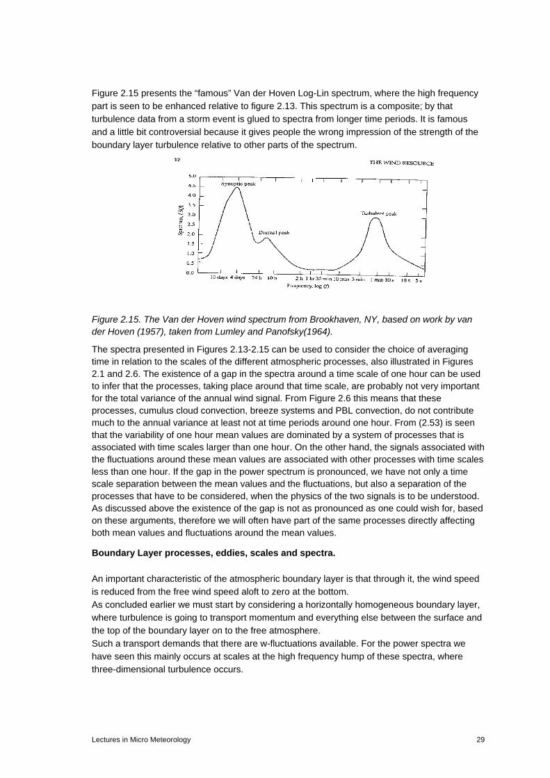
Figure 2.15 presents the “famous” Van der Hoven Log-Lin spectrum, where the high frequency part is seen to be enhanced relative to figure 2.13. This spectrum is a composite; by that turbulence data from a storm event is glued to spectra from longer time periods. It is famous and a little bit controversial because it gives people the wrong impression of the strength of the boundary layer turbulence relative to other parts of the spectrum.

Figure 2.15. The Van der Hoven wind spectrum from Brookhaven, NY, based on work by van der Hoven (1957), taken from Lumley and Panofsky(1964).

The spectra presented in Figures 2.13-2.15 can be used to consider the choice of averaging time in relation to the scales of the different atmospheric processes, also illustrated in Figures 2.1 and 2.6. The existence of a gap in the spectra around a time scale of one hour can be used to infer that the processes, taking place around that time scale, are probably not very important for the total variance of the annual wind signal. From Figure 2.6 this means that these processes, cumulus cloud convection, breeze systems and PBL convection, do not contribute much to the annual variance at least not at time periods around one hour. From (2.53) is seen that the variability of one hour mean values are dominated by a system of processes that is associated with time scales larger than one hour. On the other hand, the signals associated with the fluctuations around these mean values are associated with other processes with time scales less than one hour. If the gap in the power spectrum is pronounced, we have not only a time scale separation between the mean values and the fluctuations, but also a separation of the processes that have to be considered, when the physics of the two signals is to be understood. As discussed above the existence of the gap is not as pronounced as one could wish for, based on these arguments, therefore we will often have part of the same processes directly affecting both mean values and fluctuations around the mean values.

Boundary Layer processes, eddies, scales and spectra. An important characteristic of the atmospheric boundary layer is that through it, the wind speed is reduced from the free wind speed aloft to zero at the bottom. As concluded earlier we must start by considering a horizontally homogeneous boundary layer, where turbulence is going to transport momentum and everything else between the surface and the top of the boundary layer on to the free atmosphere. Such a transport demands that there are w-fluctuations available. For the power spectra we have seen this mainly occurs at scales at the high frequency hump of these spectra, where three-dimensional turbulence occurs.


As we notice earlier in this note, the main production mechanism is shear production, as is illustrated on the next few figures, taken from Tennekes and Lumley (1972). The first of these figures shows that the mean wind profile is unstable, continuously shedding eddies, Figure 2.16. The mean speed at two levels on each side of a given levels tend to create a whirling motion. Next figure 2.17 shows how such a motion can extract momentum (and therefore also other variables) from a mean gradient, by moving fluid elements from one level to another with other mean characteristics. This whirling motion is associated with a rotating fluid element, which we call an eddy. Figure 2.16. Development of rotation in a turbulent shear flow through overturning of air in air parcels. (Tennekes and Lumley,1972) Finally, the third figure, 2.18, shows how an eddy is stretched by the mean profile, thereby reducing its radius. This stretching also occurs by interaction between different eddies, setting up velocity gradients across each other. Aside from this stretching the velocity gradients of overlapping eddies force the eddies to shed smaller eddies corresponding to the processes associated with the mean gradients. Figure 2.17. Transfer of momentum from one level to the next by a the whirling motion derived in figure 2.16 (Tennekes and Lumley, 1972) The concept is that wind shear is continuously shedding eddies, these eddies interact with the mean shear and each other to create ever smaller eddies. We talk about an energy cascade to smaller and smaller scale. As eddies grow smaller, the velocity gradients across them become strong enough for the molecular friction to smooth out the motion. This smoothing out of motion removes variance from the wind speed fluctuations. It is called dissipation and denoted by ε.


Figure 2.18. Stretching of an eddy by the mean shear (Tennekes and Lumley,1972) The largest of these shear produced eddies are produced with scales, reflecting the scale, Λ, of the vertical shear that creates them. Close to the surface, where the vertical variation of wind speed is close to logarithmic, Λ ∼ z, the height above the ground. This eddy production with subsequent cascade down to smaller size and dissipation by viscosity has been given a poetic formulation L.F. Richardson paraphrasing a poem by Jonathan Swift.

Big whorls have little whorls, This feed on their velocity;

And little whorls have lesser whorls, and so on to viscosity.

The original

So, Nat’ralists observe, a flea Hath smaller fleas that on him prey

And these have smaller fleas to bite ‘em And so proceed to infinitum.

The swirling motion of eddies gives rise to the turbulent velocity fluctuations, the velocity variability at different eddy sizes are seen in a spectral analysis as the intensity of the power spectrum at the associated wave number.

(2.57) ( , ) ( , )ii iu t e dZ t

∞

−∞

= ∫ k rr k

(2.58) *( , ) ( , ) ( , )ij i jS t dZ t dZ t∞

−∞

′= ∫k k k

Where the subscripts refer to velocity components 1, 2 and 3.


When eddies are shed from the mean wind profile, the direction of the shear is of course important, but after a few steps in the eddy-eddy interaction involved in the cascade, the eddies have lost sense of orientation, and we say that the motion is isotropic, meaning that the flow statistics is unchanged by rotation in all directions. Since the flow cannot be truly isotropic, it is only isotropic for smaller scales, where the cascade has been active in several steps. For isotropic turbulence we can define power spectrum, E(k), being only a function of the length of the wave number vector, k, not its orientation. Below, E(k) is derived by integrating Sii(k)over all directions of the k-vector, leaving only its length as variable.

(2.59)2

( ) ( ) ,i i

ii

k k k

E k S d=

≡ ∫∫∫ k k

(2.60) 2 2 21 2 3 1 2 3

0

1 1( ) ( ) ( ( ) ).

2 2i i iiu u u u u E k dk S dk dk dk∞

= + + = =∫ ∫∫∫ k

(2.61)2 2

( )( ) ( )

4,i j

ij ij

k kE kS

k kδ

π

⋅= −k

We can separate the power spectrum into three regions as shown on figure 2.19, the production range, with k ∼1/Λ, where energy is extracted from the mean profile, a dissipation range, where the fluid motion is dissipated by viscosity, for k > η ∼ (ν3 / ε)1/4, which for typical atmospheric flows is about 1 mm. η Is called the Kolmogorov dissipation scale and is a combination of viscocity and dissipation as seen. In between there is a region, where the spectrum depends only on the wave number and the dissipation. This region is called the inertial sub-range. Since the spectrum describes wind variance per wave-number increment, it has the dimension: m3/sec2. Dissipation is destruction of variance by viscosity, hence it has the dimension of variance per second, or m2/s3. Finally, wave number has the dimension of m-1. Dimensional analysis then yields: (2.62) 2/3 5/3( )E k kαε −= Which is the “famous” Kolmogorov –5/3 law, where α is a universal non-dimensional constant, called the Kolmogorov constant, being about 0.5. In Figure 2.19, it is physically realistic to expect isotropy only within the inertial range and the dissipation range of E(k). To distinguish between such a flow and a truly isotropic flow (meaning that all scales of the flow is isotropic), we denote the boundary layer turbulence as a locally isotropic flow. The pseudo isotropic soup described by E(k) is now advected with the mean wind speed, hereby defining a coordinate system with the x1-axis along the mean speed, u, the x3 or z axis vertical with the wind speed denoted w, and the other horizontal axis, x2, with wind speed component, v, called lateral.


Figure 2.19. Schematics presentation of the energy spectrum for atmospheric boundary layer turbulence, defining the production range, with scales reflecting the mean shear, dissipation range and inertial range. (Tennekes and Lumley,1972) The component spectra now depend on how we probe, E(k). A typical way is that we use the wind speed itself, meaning that we see all the components along the mean wind speed from a stationary sensor. In (2.63) γ indicates the direction of probing specifically γ = 1 in (2.64).

(2.63) ( ) ( )ij ijS k S dγγ γ

∞ ∞

⊥−∞ −∞

= ∫ ∫ k k

(2.64) 11 2 3( ) ( )ij ijS k S dk dk

∞ ∞

−∞ −∞

= ∫ ∫ k

Or, inserting (2.60)

(2.65)

21 1

1 11 1 11 2 3 2 32 2

21 2

1 22 1 22 2 3 2 32 2

21 3

1 33 1 33 2 3 22 2

( )( ) ( ) ( ) (1 ) ,

4

( )( ) ( ) ( ) (1 ) ,

4

( )( ) ( ) ( ) (1 )

4

u

v

w

kE kS k S k S dk dk dk dk

k k

kE kS k S k S dk dk dk dk

k k

kE kS k S k S dk dk dk d

k k

π

π

π

∞ ∞ ∞ ∞

−∞ −∞ −∞ −∞

∞ ∞ ∞ ∞

−∞ −∞ −∞ −∞

∞ ∞ ∞

−∞ −∞ −∞

= = = −

= = = −

= = = −

∫ ∫ ∫ ∫

∫ ∫ ∫ ∫

∫ ∫ ∫

k

k

k 3

11 1 2 3 2 32 2

,

( )( ) ( ) ( ) ( ) 0,

4i j

ij ij ij

k

k kE kS k S k S dk dk dk dk i j

k kπ

∞

−∞

∞ ∞ ∞ ∞

−∞ −∞ −∞ −∞

⋅= = = − = ≠

∫

∫ ∫ ∫ ∫k

Notice that the cross-spectrum between any two different components is always zero, as it should be according to the assumption of isotropy, reflected by the spectrum in (2.60) From a stationary sensor, exposed to the wind, we will see a temporal signal variation that corresponds to spatial variation along the x1 axis, following Taylors hypothesis of the turbulence as given in (2.0).


(2.66)1

ut x∆ ∆

=∆ ∆

where u is the mean speed, and ∆ is the signal amplitude variation. A slightly more general formulation of Taylor’s hypothesis of frozen turbulence is that the advection speed, u, is much larger than the speed of change within the turbulence soup passing by with the wind. This hypothesis is surprisingly accurate for situations with wind larger than about 2 m/s, for the three dimensional turbulence characterising the atmospheric boundary layer, as depicted in the power spectra, presented before, meaning for frequencies larger than 0.001 Hz and horizontal wave length smaller than say 10 km. From the equation above, the relation between the wave-number, k1, wavelength, and the frequency is: (2.67) 1 2 / / 2 /k u f uπ λ ω π= = = Probing of the turbulence field, as described by E(k), along the mean wind speed, we can derive the component spectra. In the inertial sub-range one obtains, using (2.61) and (2.64):

(2.68) 2/3 5/31 1 2 3 1

4( )

3iu iS k k withα ε α α α−= = = ,

where the α’s are derived from the one universal α of the isotropic spectrum above (2.61). Also the scalar variables have inertial range forms similar to the velocity component, for example for temperature: (2.69) 1/3 5/3

1 1( ) ,T TS k N kα ε − −= where N is the dissipation rate of temperature variance, with the dimension K2 /sec. One can verify this with same dimensional analysis as for the velocity spectra. There are strong reasons to believe that the Kolmogorov constant is the same for all scalars (Hill, 1989) with αT being about 0.8. We shall in the following sections see how ε and N can be estimated from the governing equations. Overall the one- dimensional power spectra, kS(k), therefore all tend to follow a bell shape, with the –2/3 law constituting the high frequency part (at least when the dissipation range is not included). This is illustrated on the following figure 2.20. One could add that it of course is possible to probe the boundary layer turbulence along other axes than the x1, given by the mean wind speed, theoretically or using e.g. small airplanes or remote sensing. Doing so we find that the inertial ranges still holds but that the α coefficients changes, and that details in the spectra changes as well, but the overall shapes remain the same. Indeed all power spectra tend to follow a bell shape, although co-spectra have somewhat different form, as seen in Figure 2.21 that includes co-spectra as well. The spectral range, depicted in Figure 2.20 has been studied experimentally, quite intensively. Results from such measurements are exemplified in Figure 2.21 as analytical forms of power spectra and co-spectra for the three wind components and temperature based on measurements near the ground. The spectra are plotted versus the so called normalised


frequency, which is seen to correspond to the horizontal wave number multiplied by the height z, according to the Taylor hypothesis in (2.66). In boundary layer theory use this normalised frequency collapses spectra from different heights into the form shown on Figure 2.21, see section 6.

Figure 2.20. Principal sketch of the one dimensional power spectrum as function for κ1, or alternative as function of frequency, transformed to wave number using Taylors hypothesis (2.66), from Kaimal and Finigan, 1994). The power spectra of Figure 2.21 follows well the form depicted by Figure 2.20, with an inertial sub-range with a Kolmogorov constant in according with (2.67) and (2.68). The co-spectra, which for isotropic turbulence should be zero, is seen to have a significant non-zero part, carrying the fluxes, as described on p 11 and 12 in this section. At higher frequencies, all spectra approach local isotropy the power spectra approaches the predicted -2/3 –power law, while the co-spectra approaches zero much faster in according with the theory of approach to local isotropy.


Figure 2.21. Power spectra and co-spectra for atmospheric neutral turbulence close to the ground, plotted versus the normalised frequency n= fz/u ≈ zk1/2π, see (2.66), (Kaimal et al, 1972). The spectra are normalised with surface layer parameters, which together with the role of thermal stability are described closer in section 6.

The spectral formulations and the Taylors hypothesis are based on quite simple ideas, mainly of statistical nature and have been found to be so broadly valid that they are extremely useful in both experimental and modelling work. The practical limitations to the use of Taylor's hypothesis show when there is too much variation in the velocity relative to the mean flow, either due to turbulence or due to large vertical wind shear. This can influence the very low frequency, large-scale turbulence (Powell and Elderkin, 1974), and small-scale high frequency measurements (Wyngaard and Clifford, 1977; Mizuno and Panofsky, 1974, Larsen and Højstrup, 1982). The limitation to the validity of the inertial sub-range forms of the spectra is found when the assumption behind their validity breaks down, in the high-frequency end by the direct influence of the dissipation and in the low-frequency end through the direct showing of the production scales and the nearness of the surface (Tillman et al, 1994). The production scales show up in Figure 2.21 around the top of the bell shape of the power spectra, which for shear produced turbulence scale with vertical wind gradient, again scaling with the height z, as discussed on p. 24 -25 in this section. The high-frequency limit due to dissipation is illustrated on Figure 2.22. According to the discussion in connection with Figure 2.19, the dissipation becomes important for the spectrum,


strongly reducing the spectral amplitude, when kη ≥ 1, where η is the Kolmogorov dissipation scale.

fz/U Figure 2.22. Different scaled spectra near the ground shown versus the normalised frequency, fz/U (Larsen et al., 1980). 1 and 2 shows different power spectra like, u, T, u, v, or w. The hatched area , 3, represents co-spectra, while curve 4 shows a dissipation spectrum, derived from a differentiated signal as shown in section 4, (4.57) : The -2/3 slope of 1 and 2 here become represented by a +1/3 slope, followed by amplitude reduction due to dissipation.. For n <10-3, the velocity fluctuations gradually looses their 3D turbulence characteristics and become mainly horizontal fluctuations and the normalised frequency, n, loses its relevance. Hence it is common now to present spectra as function of either wave number (m-1) or frequency (Hz). However, the power spectra here still retain a kind of universality as seen in Figure 2.23, showing the spectra from multiple sources as function of frequency between 10-6 and 10-3 Hz. Noticed that the -5/3 of the inertial subrange, but not because of an inertial subrange here, describing the spectrum between the diurnal cycle and 10-3 Hz. The spectra of Figure 2.23 can be seen also in the one spectrum shown on Figure 2.14. A weaker form for Taylor hypothesis also governs the fluctuations between the diurnal cycle and 10-3 Hz in that the coefficients for the similar wave number spectrum can be found assuming advection by the mean wind of spatial fluctuations. From the diurnal cycle and down to lower frequencies, the spectrum reflects the synoptic weather patterns, and no simple relation between wave number and frequency exists, as was also discussed earlier in this section, in connection with Figures 2.6 and 2.14. The diurnal cycle, showing clearly in Figure 2.14 is in Figure 2.23 more smeared out by the many data sets, with different measuring heights. Notice also that Taylors hypothesis has no relevance for the diurnal cycle, being an exclusively a time phenomenon.

Figure 2.23. Composite plot of wind speed spectra versus frequency (Larsén et al, 2012), The “universal” spectral function, fitted to the data, is indicated. APPENDIX 2A: Correlation function integral. In this appendix we reduce the integral in (2.30)

(2A.1)

2 2 2

2 2

1 1( ( ) ) ( ( ) )2 2

1 1( ) ( ) ( )4 4

T T

TT T

T T T T

sT T T T

s t d s s t dT T

s t t s t t dt dt R t t dt dtT T

δ τ τ τ τ− −

− − − −

′= + − = +

′ ′′ ′ ′ ′ ′′ ′ ′′ ′ ′′= + + = −

∫ ∫

∫ ∫ ∫ ∫

To continue we define new coordinates, the so-called diamond transformation:

(2A.2)

; .2 2

;2 2

t t t t

and

t t

τ σ

τ σ τ σ

′ ′′ ′ ′′+ −= =

+ −′ ′′= =

(The following details are usually referred to in texts as: It is easily seen--)


The absolute value of the functional determinant for this transformation is:

(2A.3)

1 1( , ) 2 2 1.

1 1( , )2 2

t tt t

t tτ σ

τ στ σ

′ ′∂ ∂′ ′′∂ ∂ ∂= = =

′′ ′′∂ ∂ −∂∂ ∂

The integral now looks as:

(2A.4)2

2 2

1 1( ) ( 2 )4 4

T T t T t T

T s sT T t T t T

R t t dt dt R d dT T

δ σ σ τ′ ′′= =

′ ′′− − =− =−

′ ′′ ′ ′′= − =∫ ∫ ∫ ∫

The new boundaries on the other hand are complicated, and it is simpler to consider positive and negative τ separately. For positive values of τ, the σ-integration is bounded by:

(2A.5) 2 2T Tτ σ τ− − ≤ ≤ +

For negative values of τ, the σ-integration is bounded by:

(2A.6) 2 2T Tτ σ τ− + ≤ ≤ −

Figure 2A.1. Integration areas of (2.34) with the two sets of independent variables, t, t’ and (τ,σ)

. (Panofsky and Dutton, 1983)).

Hence, we can continue the integration as:


(2A.7)

22

0 2 2 2

202 2 2

2 2

20 2

1 ( 2 )4

1 ( 2 ) ( 2 )4

1 ( 2 ) .2

t T t T

sTt T t T

T T T

s sT T T

T T

sT

R d dT

d R d d R dT

d R dT

τ τ

τ τ

τ

τ

δ σ σ τ

τ σ σ τ σ σ

τ σ σ

= =′ ′′

=− =−′ ′′

+ −

− − − − +

−

− +

= =

= + =

=

∫ ∫

∫ ∫ ∫ ∫

∫ ∫

The last integral is integrated by parts:

(2A.8) 2 2 2 2

22 2

0 02 2

1 1( 2 ) 1 ( ); ( ) ( 2 ) .2 2

T T T T

T s sT T

d R d d F with F R dT T

τ τ

τ τ

δ τ σ σ τ τ τ σ σ− −

− + − +

= = ⋅ =∫ ∫ ∫ ∫

Proceeding, we now obtain:

(2A.9)

2 222

2 2 200 0

2

2

1 1 11 ( ) ( ) ( );2 2 2

( ) ( 2 ) .

T TT

T

T

sT

d F F d FT T T

with F R dτ

τ

δ τ τ τ τ τ τ ττ

τ σ σ−

− +

∂= = ⋅ = − ⋅∂

=

∫ ∫

∫

The first term is seen to be zero in both limits. Hence we can write: (2A.10)

22

20

2 2

20 2

2 2

2 20 0

1 ( )2

( 2 ) ( 2 )1 ( 2 ) (2 2 ) (2 2 )2

1 10 (2 2 ) ( 2 2 ) (2 2 );2

T

T

T T

s s sT

T T

s s s

d FT

T Td R d R T R TT

d R T R T d R TT T

τ

τ

δ τ τ ττ

τ ττ τ σ σ τ τ

τ τ τ

τ τ τ τ τ τ τ

−

− +

∂= − ⋅

∂

∂ − ∂ − +∂ = − ⋅ + − − − ∂ ∂ ∂

= − ⋅ − − − − + = ⋅ ⋅ −

∫

∫ ∫

∫ ∫

Once more we substitute: ξ = 2T-√2 τ, with dξ= -√2 dτ:

(2A.11)2

2

0

1 (1 ) ( ) .2

T

T R dT T

ξδ ξ ξ= −∫

Introducing the autocorrelation function ρs(τ), and changing ξ to τ, this expression can be written:

(2A.12)2 2

2

0

(1 ) ( )2

Ts

T s dT T

σ τδ ρ τ τ= −∫


3. Basic equations

Our objective is here to establish useful equations for our main atmospheric variables with suitable simplifications. Variable: Pressure, p. Density, ρ. Composition: here we shall distinguish between the density of dry air and ρd and the density of water vapour, ρw. .Other trace constituents are not dynamically important, and will considered as passive tracers in the atmosphere. Temperature: T, and velocity; ui = u1, u2, u3. Complications: We are on a rotating planet, meaning that we seek to interpret the motion in a rotating (accelerating) coordinate system. Additional there is a variation of p, ρ, T with height induced by gravity. We start considering 7 parameters, because we have two densities, for water vapour and for dry air.

Equation of state

The ideal gas law:

(3.1) .p RTρ= Since, both R and ρ depend on the composition, we decompose (3.1) into its partial pressure for dry air and water vapour.

(3.2) 0 0 ,d w d wd w

R Rp p p T T

M Mρ ρ= + = +

where R0 is the universal gas constant and M is the molecular weight for the gas considered.

Notice: ρ = ρd + ρw. We use the definition for mixing ratio, q ≡ ρw/ρ. We can rearrange (3.2) to:

(3.3) 0 (1 ( 1) ) :d

d w

R Mp T q or

M Mρ= + −

(3.4) ; (1 0.61 ).d v vp R T T T qρ= ≡ + Writing the equation as above means, we treat the atmosphere, as it was dry air only, with respect to ρ, p and R. As a penalty we have to operate with and artificial temperature, Tv, denoted the virtual temperature. Note that typically q << 0.1 kg/kg. Vertical variation of p and ρ: Consider first a hydrostatic balance between the weight of a volume of air and the pressure force on this volume.

(3.5) ,p

gz

ρ∂

= −∂

where we have balanced the forces due to gravity and due to pressure. Inserting the equation of state (1.1) and assuming an isotherm atmosphere, we can write, e.g.:

(3.6) p p g pz RT H∂

= − ≡ −∂

where H is called the scale height, typically about 10 km. With g ≈ 9.81 m/s2, T ≈ 288 K and R ≈ 287 J K-1 kg-1. Thereby H becomes 8.4 km. The two equations of course allow for solutions also for more realistic variations of T. Comparing with atmospheric data on the height variation of pressure and temperature, we find that while the measured pressure depends roughly as the exponential decay predicted by (3.6), the temperature variation is very different from the constant assumption used, with different behaviour in the different layers of the atmosphere. The height variation of pressure and temperature also influences the dynamic stability of the atmosphere. To see this we shall move an air parcel vertically. Consider figure 3.1, where we move an air-parcel up- and down in an atmosphere with vertical structure ruled by the hydrostatic equation between density and pressure changes. As we move the air parcel, it will change it volume, V and thereby its density in response to the external pressure found at its new position. We now assume the motion of the air parcel to be too fast for the parcel to exchange heat with its surroundings on the way to a new position. This means that the changes of the internal parameters in the parcel, ρ, Τand p, are controlled by an adiabatic process. In the following we shall distinguish between parameters internal to the parcel, denoted by subscript i, and parameters pertaining to the surrounding atmosphere, without subscript. For our adiabatic parcel parameters we have:

(3.7) ;

:

ii p

i

ii

i

dp CdT

pAlsoRT

ρ

ρ

=

=

where Cp is the heat capacity, or specific heat, ~1010 (JK-1kg-1) at constant pressure


.

p

ρi3,Ti3,pi3

ρi2,Ti2,pi2

ρi1,Ti1,pi1

p(z), ρ(z), T(z).

,p gz

ρ∂= −

∂

Figure 3.1 Adiabatic vertical motion of an air parcel in a hydrostatic atmosphere. As the air parcel is moved to a new position it adapts to surrounding pressure with the speed of sound (that is instantaneously). If the air parcel has moved dz the external pressure has changed in according with the hydrostatic balance by: (3.8) dp gdzρ= − The internal pressure has similarly changed, ruled by the adiabatic equation: (3.9) .i i p idp C dTρ= Assuming now that the air parcel starts out from equilibrium between parcel variables and the surrounding variables: ρ i ∼ρ. As discussed above dpi = dp. Combining the equations for the external and the internal changes, we obtain:

(3.10) 0.01 / 1 /100 ,i

p

dT g K m K mdz C

=− ≡− Γ ≈ =

where we have defined the dry adiabatic lapse rate, Γ. Until now, we have considered only the changes in an air parcel. Now consider an air parcel moving up and down in three different vertical temperature gradients, being in equilibrium with the surroundings in position (a), and moving to the points (b) and (c). We assume the pressure to be the same for all three situations. The internal parameters of the air parcel will always develop following the dry adiabatic lapse rate, as seen on the figure.


.

Th i l f h i l ill l d l

z

T

b

a

cT1(z)

T3(z)T2(z) =T0 -Γz

Figure 3.2 Air parcel moving adiabatically up and down in an atmosphere with different thermal stratifications. If the air parcel moves in the T2(z)-atmosphere, it is seen to be in equilibrium also at the new heights, b and c. If the air parcel moves in the T1(z)-atmosphere: Starting at level c and arriving at level (b) the air parcel will be warmer and therefore lighter than the surrounding air. Arriving at level (c) it will correspondingly be colder and hence heavier than the surroundings. Hence, all motion initiated will continue. If the air parcel moves in the T3(z)-atmosphere, starting at level a, and arriving at level (b) the air parcel will be colder and thereby heavier than the surroundings. Arriving at level (c) it will be warmer than the surroundings and hence lighter. Hence, an initiated motion will be counteracted by the buoyancy forces. Based on this image, we call the T2(z) - temperature stratification for neutral, because it will not influence initiated motion. The T1(z)-atmosphere is called unstable, because all initiated motion will be amplified. The T3(z)-atmosphere is called stable, because all initiated motion will be damped by the temperature stratification. Hence, such stratification stabilises existing situations. Potential temperature The potential temperature,θ, is defined as the temperature an air parcel acquires, when it is moved adiabatically to a reference pressure level, p0. Since much air motion involves adiabatic motion, we see that air parcels will retain their potential temperature during most motions, meaning that potential i for many situations can be considered a conservative aspect of an air parcel. From (3.7) we have:

(3.11) ;

:

ii p

i

ii

i

dp CdT

pAlsoRT

ρ

ρ

=

=


Recalling that p always equalises instantaneously with the surroundings, combination of these two equations we get: (3.12) i i

p i i p

dp dT dpR RC p T C p

==

Ti,pi,ρi

pi= p0Ti = θ,

Figure: 3.3. Definition of potential temperature. We now follow the air parcel down to the reference level:

(3.13) 0

.p

i

i pT p

dT R dpT C p

θ

=∫ ∫

or:

(3.14)

0

0

ln( ) ln( ),

( ) .p

p

RC

pRT C p

orpTp

θ

θ

=

=

Notice that the only parameter reflecting parcel parameters is θ ≡ θ i because the air parcel is in equilibrium with the surroundings before it is moved to level, p0, and we assume continuous pressure equilibration. The equation is called Poisson’s equation. It is seen that every parcel of air has a unique potential temperature that is conserved for dry adiabatic motion. We say that θ can be called a conservative quantity, because it does not change, when an air parcel is moved around, as opposed to the real temperature that changes when the air parcel is moved adiabatically up-or down, as discussed above. Since p and T are functions of height z, so is θ, meaning that θ is a function of the height from which we start moving an air parcel “down” to the reference level. Differentiating (3.14) with respect to z we obtain, using the hydrostatic balance:


(3.15)

10 0 02( ) ( )

.

p pR R

C C

p

p p

p p pT R pTz z p C p zp

T R T p T R T pgT z C p z T z C p RT

TT z

θ

θ θ

θ

−∂ ∂ ∂= − =

∂ ∂ ∂

∂ ∂ ∂ −= − = − = ∂ ∂ ∂

∂ = + Γ ∂

We assume that the reference level in the boundary layer is at the surface, z = 0, where then θ = T. Throughout the total boundary layer, we therefore have θ ≈ T ≈ 300 K. Hence, we see that

(3.16) ; ( ) ( ) .T z T z zz zθ θ∂ ∂≈ + Γ ⇒ = +Γ

∂ ∂

Returning to the concept of stability, we see that it can be characterised two ways, using the temperature or using the potential temperature. For each temperature gradient, the characteristic of the atmosphere is shown in parenthesis.

(3.17) ( ), ( ), ( ).T neutral or unstable or stablez

∂=−Γ <−Γ >−Γ

∂

or:

(3.18) 0( ) , 0( ) , 0( ).neutral or unstable or stablezθ∂= < >

∂

For a neutral dry boundary layer the temperature falls with about 1 K/ 100 m. Note further that for adiabatic motion, the potential temperature of an air parcel is unique. We next turn to the complications from humidity. If water vapour is present the equations we have to consider look as follows:

(3.19) ( ) ;( )

i i ii p i i

i vi i

dp p pC q or and dp gdz

dT RT R q Tρ ρ ρ ρ= = = = −

with: Tv = T(1+0.61q). Formally, (3.19) can be written in the same way as the equations for dry conditions, see (3.14):

(3.20) ( )( ) ( )d i i i i

p i vi p i i

R dp dT dp dTR qor alternativelyC q p T C q p T

= =

However, (3.20) cannot be integrated in a unique way anymore, because the integral now depends on the path to the reference level, and the variation of humidity along that path. Only if we assume that q is a constant, can we integrate.

If q is constant, we can choose to integrate with respect to T or Tv. If we do the first, we arrive to that the atmosphere is neutral if:

(3.21) ( ), ( ) .dT

q where qdz

=−Γ Γ <Γ

For a typical “moist” atmosphere, one finds that the temperature decreases with about 0.5 K per 100 meter, not the dry adiabatic decrease of 1 K/100m. This moist adiabatic variation included as well face changes between water and water vapour. If we integrate with respect to Tv, we arrive to that we can define a virtual potential temperature similarly to the potential temperature. (3.22) (1 0.61 ) ( )v vq T q zθ θ= + = + Γ Equations of motion We shall now derive a suitable set of equations for wind, temperature and other scalars. We start by deriving Euler’s equation relating partial and substantial derivatives. Euler’s equation We consider a volume V that moves through space, meaning that its position can be given as (x (t), y (t), z (t)). Assume that we have a field ϕ = ϕ(x,y,z,t). We wish to determine the changes in ϕ within the volume as it moves through space. This means we consider ϕ(x (t), y (t), z (t), t). We change to write the coordinates as (xi (t), t). We track the change as the volume moves from (xi (t), t) to (xi (t + δt), t + δt), where i = 1, 2, 3. (3.23) ( ( ), ) ( ( ), ).i ix t t t t x t tδϕ ϕ δ δ ϕ= + + − We use Taylor expansion:

(3.24) 2 2

2

( )( ( ), ) ( ( ), ) ( ( ) ( ))

2i i i ii

tx t t t t x t t x t t x t t

x t tϕ ϕ ϕ δ

ϕ δ δ ϕ δ δ∂ ∂ ∂

+ + = + + − + + − − − + +∂ ∂ ∂

,

We now divide by δt, and let it go to zero:

(3.25) 2

2

( ( ), ) ( ( ), ) ( ( ) ( )) ( )2

i i i i

i

x t t t t x t t x t t x t tt x t t t

ϕ δ δ ϕ δϕ ϕ ϕ δδ δ

+ + − + −∂ ∂ ∂= + + − − − + +

∂ ∂ ∂

When letting δt→0, we notice that:

(3.26)

( ( ), ) ( ( ), )0;

( ( ) ( ))0;

i i

i ii

x t t t t x t t dfor t

t dtx t t x t

u for tt

ϕ δ δ ϕ ϕδ

δ

δδ

δ

+ + −→ →

+ −→ →

where up is the velocity of our volume. Hence, we arrive at Euler’s equation relating total derivatives to partial derivatives:

(3.27) ;ii

d u u v wdt t x t x y z tϕ ϕ ϕ ϕ ϕ ϕ ϕ ϕ ϕ∂ ∂ ∂ ∂ ∂ ∂ ∂= + = + + + = + ⋅∇∂ ∂ ∂ ∂ ∂ ∂ ∂

u

This relation will be used extensively in the following and is shown here in its different forms. The continuity equation We express that in a stationary volume of dry air in space, changes in density can only happen through transport in and out of the volume.

ρ2u2ρ1u1

x1 x2

q y

Figure 3.4. Density change in a volume of air, note the copied figure operates in (x,y,z) and increments in these . Consider the change of density due to the net flux in the u direction: (3.28) 2 1 2 2 1 1( ) ( )x x u u tρ ρ ρ∆ − = − − ∆

(3.29) 2 2 1 1( )u ut x

ρ ρρδ−∆

=∆

Letting both ∆t and δx go to zero yields:

(3.30) ( )ut xρ ρ∂ ∂=−

∂ ∂

Going to 3D we now get:

(3.31) ( ) ( ) ( )

0i ii

i i i

u uu

t x t x xρρ ρ ρ

ρ∂ ∂∂ ∂ ∂

+ = = + +∂ ∂ ∂ ∂ ∂

We can now use Euler’s equation:

(3.32) ii

du

dt t xϕ ϕ ϕ∂ ∂= +∂ ∂

,

and write an alternative form of the mass balance, for a volume following the flow:


(3.33) 0i

i

uddt xρ

ρ∂

+ =∂

This equation can be interpreted in terms of non-compressibility. The equation shows that if:

(3.34) 10

ddtρ

ρ≈

Then

(3.35) 0 0.i

i

uor

x∂

= ∇ ⋅ =∂

u

Note, that the argument is somewhat weak. Because the assumption is not consistent with the result:

(3.36) 10i

i

uddt xρ

ρ∂

<< =∂

A more thorough derivation must utilise scale arguments about the possible rate of change for the two terms (Mahrt, 1986). The momentum equation To derive the momentum equation, we start with Newton’s second law for a fluid element:

(3.37) 1,2,3jii

j

dum F with idt

= =∑

Where, m = mass, ui = component i of the velocity and F i j is component i of force, j. To proceed we have to identify the different forces Fi j and also to describe the effect of having a rotating coordinate system, where the rotation considered is the rotation of the Earth. This is done in the following equation, where we consider a unit volume, and hence denote the mass by, ρ:

(3.38) 3 2 ;ii ijk j k i

i

du pg u F

dt x

I II III IV

ρ ρ δ ρ ε η∂

= − − − Ω +∂

Where, we have identified different forces (one being a virtual force). Below we discuss the term one by one: I: The gravitational force is in the vertical, indicated application of the Kroneker- δ, which is equal to 1 with the two subscripts being equal and 0, if the subscripts are different. II: The pressure force. Here we have already seen the vertical pressure force, balancing gravity in hydrostatic equilibrium.

III: Coriolis force, which is not a force, but appears because we consider the equation in a moving frame of reference given by the rotating Earth. The term derives from 2Ω(η×u), η is a unit vector parallel to Earth rotation and Ω is the angular frequency of rotation.ε ijk is a cyclic operator , being +1, -1 dependent on the order of i, j and k and 0 if two of the indices are equal. Term I includes as well a small component from the rotation. When describing the motion in its components, we must specify the components of η in our chosen local coordinate system. Here we will chose different systems during our excursions into boundary layer flows. However they will all have an x1 and x2 that are horizontal, x3 is vertical, and we can therefore find the x3 component of η to be equal to sinϕ, where ϕ is the latitude. Fortunately the expressions for η1 and η2 will not be important, as we shall see. Since, η3 will enter the important part of this term we will already now define the so-called the Coriolis parameter: fc = 2Ω sinϕ, which depends on latitude. For mid- latitude, fc ≈ 1.45 10-4 s-1. At equator it is zero.

xj

Xi

τij

The viscous stress τijattacks a plane ∟ to xjin the direction of xi

Figure 3.5. Specification of viscous or shearing stress,τ ij, across a plane perpendicular to xj and in the direction of xi.

IV: The friction force F on an air parcel is produced by the viscous force or shearing stress, τ ij ,

across the fluid element considered in the figure above. The stress is a tensor, τ ij, where element i,j attacks a plane perpendicular to xj in the direction of xi , see figure. The stress is due to the movements and interactions of molecules across the boundaries of the fluid element. The shearing stress is normally assumed to be proportional to the velocity gradients:

(3.39) ( )jiij

j i

uux x

τ µ∂∂

= +∂ ∂

,

which is a general expression assuming that the shearing stress is linearly proportional to the shear, when we assume incompressibility. µ is denoted the dynamic viscosity. For the simplest situation with a positive ui gradient in the j-direction and no uj gradient it is easy to describe what happens, from the molecular viewpoint a positive the shearing stress in the i-direction results from a net downward transport of ui- momentum by the random motion of the molecules. Because the ui-momentum increases in the xj direction, the molecules passing downward through a horizontal plane perpendicular to xj at any instant carry more momentum than those


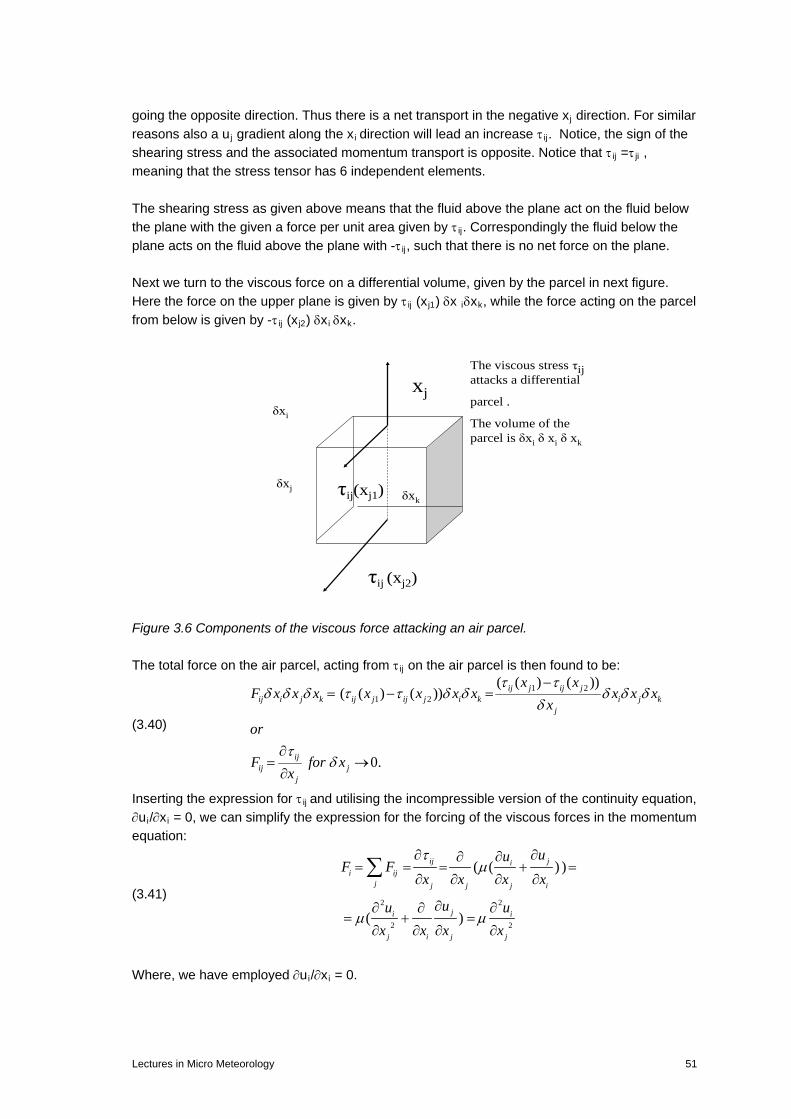
going the opposite direction. Thus there is a net transport in the negative xj direction. For similar reasons also a uj gradient along the xi direction will lead an increase τ ij. Notice, the sign of the shearing stress and the associated momentum transport is opposite. Notice that τ ij =τ ji , meaning that the stress tensor has 6 independent elements. The shearing stress as given above means that the fluid above the plane act on the fluid below the plane with the given a force per unit area given by τ ij. Correspondingly the fluid below the plane acts on the fluid above the plane with -τ ij, such that there is no net force on the plane. Next we turn to the viscous force on a differential volume, given by the parcel in next figure. Here the force on the upper plane is given by τ ij (xj1) δx iδxk, while the force acting on the parcel from below is given by -τ ij (xj2) δxi δxk.

xj

τij(xj1)

The viscous stress τijattacks a differential

parcel .

The volume of the parcel is δxi δ xi δ xk

τij (xj2)

δxi

δxk

δxj

Figure 3.6 Components of the viscous force attacking an air parcel. The total force on the air parcel, acting from τ ij on the air parcel is then found to be:

(3.40)

1 21 2

( ( ) ( ))( ( ) ( ))

0.

ij j ij jij i j k ij j ij j i k i j k

j

ijij j

j

x xF x x x x x x x x x x

xor

F for xx

τ τδ δ δ τ τ δ δ δ δ δ

δ

τδ

−= − =

∂= →∂

Inserting the expression for τ ij and utilising the incompressible version of the continuity equation, ∂ui/∂xi = 0, we can simplify the expression for the forcing of the viscous forces in the momentum equation:

(3.41) 2 2

2 2

( ( ) )

( )

ij jii ij

j j j j i

ji i

j i j j

uuF F

x x x x

uu ux x x x

τµ

µ µ

∂ ∂∂∂= = = + =

∂ ∂ ∂ ∂

∂∂ ∂∂= + =

∂ ∂ ∂ ∂

∑

Where, we have employed ∂ui/∂xi = 0.


The momentum equation now takes the form:

(3.42) 2

3 22 ;i ii ijk j k

i j

du upg udt x x

ρ ρ δ ρ ε η µ∂∂

= − − − Ω +∂ ∂

or dividing with ρ :

(3.43) 2

3 2

1 2 ;i ii ijk j k

i j

du upg udt x x

δ ε η νρ

∂∂= − − − Ω +

∂ ∂

where ν is called the kinematic viscosity. For air ν ≈ 1.5 10-5 m2 s-1 = 0.15 cm2/s. Mass balance for a scalar We denote the scalar concentration by C, which we can either think upon as mass per volume [kgm-3], or as mixing ratio [kg-C/kg-Air]. The change of C in a volume following the wind speed can be found from:

(3.44) .Ci

i

FdCSources Sinks

dt x∂

= − + −∂

;

where FCi is the flux of C along the direction of xi, see figure, where the mass changes due to a gradient in FCi across a volume is computed, including an internal net source, SC[ Cs-1].

FCi1FCi2

Xi1 Xi2

δX1 = Xi2 – Xi1

δC

Figure 3.6. Change in concentration of scalar C in a volume with fluxes.

(3.45) 1 2

;

( ) ;i j k C i C i j k i j k

S Sources Sinks

C x x x F F x x t S x x x tδ δ δ δ δ δ δ δ δ δ δ

= −

= − +

Dividing by the differential volume and δt, one obtains


(3.46) 1 2( ) ( )0.C i C i C i

i i

F F FC dCS S for

t x dt x

δδ

δ δ

− ∂= + → = − + →

∂

To proceed we need to describe the flux, F. Since we follow the flow, the time derivative of the concentration C must be substantial, and the flux in/out of our volume must be associated with the molecular motion. Also here we often assume the flux in a point to go from high towards low concentration. We can then either say we assume the flux to be linearly proportional to the gradient of the concentration, or consider it a Taylor expansion of the concentration variation across the point, and then consider only first order.

(3.47) Ci Ci

CF kx∂

= −∂

,

where kc is the molecular diffusivity of the substance C in the atmosphere. This type of assumption about fluxes is used throughout physics, especially for Fluid Mechanics and molecular gas theory. It is not always true, and we shall in boundary layer descriptions see several cases where one has been forced to reformulate the theories because the assumption does not hold. From molecular gas theory we have:

(3.48) 2C C Ck a v≈ ,

where a is a coefficient, and kC is assumed proportional to the standard deviation of the velocities of the C- molecules in the atmosphere, while lC is the mean free path between the same molecules. Notice, the first term will change with temperature, while the last will change with pressure. The changes over temperature and pressure ranges of relevance for the atmospheric boundary layer are however so small that kC is considered constant here.

(3.49) 2

2i C Ci i i i

dC C C C Cu k S k Sdt t x x x x

∂ ∂ ∂ ∂ ∂= + = + = +∂ ∂ ∂ ∂ ∂

From the budget for a scalar, we can derive the equation for the potential temperature:

(3.50) *2

2

1 jj T

j j p p j

Qd LEu kdt t x x C C xθ θ θ θ

ρ ρ∂∂ ∂ ∂

= + = − −∂ ∂ ∂ ∂

,

Where, kT is the thermal diffusivity, corresponding to kC above. kT is about 2.16∙10-5 m2/s , about 1.44 larger than the kinematic viscosity. Additionally, we have in (3.50) introduced two specific terms in the source, S. The first will be relevant, if water is present in the atmosphere as both liquid and vapour phases. E is the water vapour production from evaporation of liquid water within the volume, i.e. from droplets. L is the coefficient of evaporative heat consumption. Cp is the heat capacity at constant pressure of the air. The other source term that can be important in the atmospheric boundary layer is the divergence of the net-radiation, Qj* in the j-direction.


It should be noted that derivation of the equation for the potential temperature is fairly complicated starting from conservation of enthalpy. We avoid this derivation here, but we note that the simplicity of the equation demands that it is formulated in terms of potential temperature. Had we instead derived an equation for the temperature, T, we would have to include terms explaining how the temperature changed due to changes in pressure for vertical transport, as considered when deriving expressions for potential temperature above (3.10-3.22). If only horizontal motion is considered the equations for T and θ become the same. In the spirit of keeping track of both liquid and gaseous water, we must keep track on both phases of the water:

(3.51) ( ) ( )

T Lmass of liquid mass of vapourq q q

mass of air +

≡ + =

,

As qT is a scalar quantity its budget equation can be written:

(3.52) 2

2qTT T T

j qj j

Sdq q q qu kdt t x x ρ

∂ ∂ ∂= + = +

∂ ∂ ∂,

where SqT is the net source of total water in the air, for example by water droplets being injected into the volume, and by evaporation of such droplets. We write: SqT = Sq + SqL, separating S in a source term for vapour and for liquid. kq is the molecular diffusivity of water vapour in the air. Notice, we imagine that there is no diffusion of liquid water vapour the boundaries of the differential volume. Hence we can write the equations for the two phases of the water:

(3.53)

2

2 ;

.

qj q

j j

qLL L Lj

j

Sdq q q q Eu kdt t x x

Sdq q q Eudt t x

ρ ρ

ρ ρ

∂ ∂ ∂= + = + +∂ ∂ ∂

∂ ∂= + = −

∂ ∂

In general we will neglect these aspects of water and water vapor. Note Sq and E will often be combined. Similar issues arise when a species, C, is not passive but chemically/ or radioactively active, meaning that there are sources and sinks, in the volume, independent of the turbulence transport. We shall not go further into this but refer to Lenschow and Delany (1987) and Kristensen et al (2010) for studies involving chemical reactions, and Fairall and Larsen (1984) and results involving aerosols. Summary of equations and averaging considerations. We have now established the necessary 8 equations to handle our 8 unknowns. T, u1, u2, u3, q, θ, ρ and p Equation of state: (3.54) , (1 0.61 ).d v vp R T withT T qρ= ≡ +

Relation between T and θ:


(3.55) T zθ = + Γ Continuity equation, in the incompressible mode:

(3.56) 0;j

j

ux∂

=∂

The momentum equation:

(3.57) 2

3 2

1 2 ;i i i ij i ijk j k

j i j

du u u upu g udt t x x x

δ ε η νρ

∂ ∂ ∂∂= + = − − − Ω + ∂ ∂ ∂ ∂

Temperature:

(3.58) *2

2

1 jj T

j j p p j

Qd LEu kdt t x x C C xθ θ θ θ

ρ ρ ∂∂ ∂ ∂

= + = − − ∂ ∂ ∂ ∂

Water vapour:

(3.59) 2

2j qj j

dq q q q Eu kdt t x x ρ

∂ ∂ ∂= + = + ∂ ∂ ∂

Since we cannot solve these equations directly, we wish to derive equations for the mean quantities, in keeping with our discussion in section 2. In the equations above we have used [ ] to indicate the non-linear terms, i.e. terms where we have products or ratios of two variables. From the discussion of the averaging procedures in chapter 2, we must expect complications for these terms, while the other terms are linear and will behave nicely, when we average. To solve the equations for the average variables, we must expect to have to consider also equations for the fluctuations. Therefore we now wish to simplify the equations such that the average equations can be obtained more easily, while the equations for the fluctuations are still useful as well. The method we use for generating equations for the mean values is to insert the variables, decomposed into averages and fluctuations, and then average the equations (afterwards we derive equations for the fluctuation by subtracting the mean equations from the equations for the raw variables. (3.60) ; ; ; ; ;i i iu u u p p p q q qθ θ θ ρ ρ ρ′ ′ ′ ′ ′= + = + = + = + = +

We neglect the linearity problems associated with the E-terms in temperature and humidity equations, and the radiation term in the temperature equation. Thereafter, we have two types of non-linearity, the one is associated with the advection term in all equations, while the other is associated with the pressure term in the momentum equation. We consider the last of these.

(3.61) 2

3 2

1 2 ;i ii ijk j k

i j

du upg udt x x

δ ε η νρ

∂∂= − − − Ω + ∂ ∂

Consider the first two terms on the right hand side:

(3.62) 31

i ii

pY gx

δρ∂

=− −∂


We will now study the possibility for linearising Yi for small values of the p’ and ρ’, without removing too much information for both average equations and fluctuation equations, because we know from the start of the section that the vertical stratification of p and ρ are very important for the flow characteristics. Also, we shall see if p’, and ρ’ can really be considered small enough for linearization. To the first order in the fluctuations we may write:

(3.63) 3 3

3

( ) ( )1 1 (1 )

( ) ( )1 1 .

i i ii i

ii i

p p p pY g gx x

p p p pgx x

ρδ δρ ρ ρ ρ

ρδρ ρ ρ

′ ′′∂ + ∂ +=− − ≈− − − =

′+ ∂ ∂′ ′′∂ + ∂ +

=− − +∂ ∂

We will now evaluate these terms for i = 1, 2 and i = 3 separately, i.e. the vertical and the horizontal components separately. i =3

(3.64) 3( ) ( ) ( ) ( )1 1 1 1p p p pY gz z z z

ρ ρρ ρ ρ ρ ρ ρ

′ ′′ ′∂ ∂ ∂ ∂= − − − + +

∂ ∂ ∂ ∂.

Now assume the hydrostatic equation is at least approximately valid for the mean values of p and ρ, and evaluating the terms to first order only ( i.e. removing the last term in (3.64).

(3.65)

31 ( ) 1 ( ) 1 ( )

1 ( ) 1 ( ) 1 ( )

1 ( ') 1(1 ) (1 );

p p pY gz z z

p p pgz z z

p p pg gz z

ρρ ρ ρ ρ

ρρ ρ ρ ρ

ρ ρρ ρ ρ ρ

′ ′∂ ∂ ∂= − − − +

∂ ∂ ∂′ ′∂ ∂ ∂

= − − − +∂ ∂ ∂

′ ′∂ + ∂=− − + = − − +

∂ ∂

As seen, first order terms in the fluctuations are the lowest order terms that remains, because the average terms cancels-at least approximately due to the hydrostatic balance. Therefore, we should here keep the whole last term and not neglect ρ’/ρ relative to 1. i = 1,2 Here we can safely neglect ρ’/ρ relative to 1.

(3.66) 31 ( ) 1 ( ) 1(1 ) ;i i

i i i

p p p p pY gx x x

ρδρ ρ ρ ρ ρ

′ ′ ′∂ + ∂ + ∂=− − ≈− − ≈ −

′+ ∂ ∂ ∂

For both these equations, we must evaluate the importance of the first order terms, especially the term containing the fluctuating density, ρ’/ρ. Consider the equation of state:


(3.67) ln ln ln ln .v dd v

p or p T RR T

ρ ρ= = − −

Differentiation yields:

(3.68) v v

v v

dT Td dp porp T p T

ρ ρρ ρ

′′ ′= − = − ,

Where, we have associated differentials with the fluctuations, reflecting that the fluctuations in the parameters here are small compared to the mean values. Exactly how small they are will depend on the overall atmospheric conditions. However, the data indicate:

(3.69) 3 3( ) 10 ; ( ) 4 10 .v

v

TpO Op T

− −′′

≈ ≈ ⋅

Hence:

(3.70) ,v v

v v

TT

θρρ θ

′ ′′≈ − ≈ −

Where, we have introduced the virtual potential temperature to generalise the result. If we assume the reference level for the potential temperature to be the surface it is seen that the mean values for the potential temperature and the virtual potential temperature are very close to each other since they only differ with Γ(q)z, and with z small that term is small compared to 300K. The fluctuations are the same since Γ(q) z does not fluctuate statistically. Note the order of magnitude evaluation of the importance of the pressure and the temperature terms do not indicate a large difference, hence we can under special circumstances expect the pressure terms to become important. However, for now we conclude that the temperature term dominates the density fluctuations, and that the relative density fluctuations generally must be considered so small that they can be neglected compared to one. For i = 1, 2 we can therefore write:

(3.71) 1 ( ) 1 ;i

i i

p p pYx xρ ρ

′∂ + ∂≈ − ≈ −

∂ ∂

However, for i =3, it is seen that the leading terms are cancelled by the hydrostatic equation, and the relative density fluctuations become multiplied by g, and therefore can be strong enough to influence the equations for the fluctuations. Therefore theY3 takes the form (3.65). Hence, we write the momentum equation on the form:

(3.72)

2

3 2

1(1 ) 2 ;i i i v ij i ijk j k

j v i j

du u u upu g udt t x x x

I II III IV V VI

θδ ε η ν

θ ρ′∂ ∂ ∂∂

= + = − − − − Ω +∂ ∂ ∂ ∂

In this equation we have removed one non-linearity from the momentum equation. We now proceed to insert the Reynolds’s convention for fluctuations and mean values and then take the mean value of the terms in the equation. We proceed term by term: term I:


(3.73) ( ) ( )

;i i i i iu u u u ut t t

′ ′∂ + ∂ + ∂= =

∂ ∂ ∂

Term II:

(3.74)

( )( )

( ) ;

i i i i i i i ij j j j j j j j

j j j j j j j

i ij j ji ij i j

j j j j j

u u u u u u u uu u u u u u u u

x x x x x x x

u u u uuu uu u u

x x x x x

′ ′ ′ ′∂ + ∂ ∂ ∂ ∂ ∂ ∂′ ′ ′ ′+ = + + + = +

∂ ∂ ∂ ∂ ∂ ∂ ∂

′ ′ ′ ′′∂ ∂∂∂ ∂′= + − = +

∂ ∂ ∂ ∂ ∂

where we have repeatedly used the continuity equation in its various forms:

(3.75) 0; 0; 0;j j j

j j j

u u ux x x

′∂ ∂ ∂= → = → =

∂ ∂ ∂

As is seen all the other terms in the momentum equation are linear in the variables. The procedure then proceeds as for the time derivative above. Term III:

(3.76) 3 3(1 )vi i

v

g gθ

δ δθ′

− =

Term IV

(3.77) ( ) ( )1 1 1

i i i

p p p p px x xρ ρ ρ

′ ′∂ + ∂ + ∂= =

∂ ∂ ∂.

Term V: (3.78) 2 2ijk j k ijk j ku uε η ε ηΩ = Ω Term VI:

(3.79) 2 2 2

2 2 2

( );ii i i

j j j

u u u ux x x

ν ν ν′∂ ∂ + ∂

= =∂ ∂ ∂

Therefore we can now write the equation for the mean velocity components:

(3.80) 2

3 2

1 2 ;i i i ij i ijk j k j

j i jj

du u u upu g u u udt t x x xx

δ ε η νρ

∂ ∂ ∂∂ ∂ ′ ′= + = − − − Ω + −∂ ∂ ∂ ∂∂

With the momentum equations processed, it is easy to summarise all the equations for the mean variables (C is a scalar concentration, i.e. (3.49)):

(3.81) , 1, 2,3; ; ; ; ; , .i i iu u u i T p p p q q q C C Cθ θ θ ρ ρ ρ′ ′ ′ ′ ′ ′= + = = + = + = + = + = +

Continuity:

(3.82) 0;i

i

ux∂

=∂

Momentum:


(3.83) 2

3 2

1 2i i i ij i ijk j k i j

j i jj

du u u upu g u u udt t x x xx

δ ε η νρ

∂ ∂ ∂∂ ∂ ′ ′= + = − − − Ω + −∂ ∂ ∂ ∂∂

;

Potential temperature:

(3.84) *2

2

1 jj T j

j j j p jp

Qd LEu k udt t x x x C xCθ θ θ θ θ

ρ ρ∂∂ ∂ ∂ ∂ ′ ′= + = − − −

∂ ∂ ∂ ∂ ∂;

Water vapour:

(3.85) 2

2 ;jj q

j jj

u qdq q q q Eu kdt t x xx ρ

′ ′∂∂ ∂ ∂= + = − +∂ ∂ ∂∂

Any Scalar:

(3.86) 2

2 ;jj C

j j j

u CdC C C Cu k Sdt t x x x

′ ′∂∂ ∂ ∂= + = − +∂ ∂ ∂ ∂

It is seen that we have 9 variables and 7 equations above. The remaining equations are the equation of state and the relation between T and θ . Note that we consider E and Q* and S as externally given variable. Also, we have neglected that strictly Cp varies with the humidity content of the air. In general the equations for the average variables have retained the original form for the raw variables, with one important exception that a number of correlation terms involving the fluctuations enter into the equations. Their origin is the non-linearity of the advection terms. One result of this is that we end up with equation with more variables than we started with for the raw variables. This is called the “closure problem” and is the theme of chapter 4. The physical meaning of the correlation terms is that they constitute a change in the average variable due to a divergence of a turbulence flux. Recall that we have seen that a correlation involving a velocity component can be interpreted as a flux along the line of the velocity component. As noticed above we have avoided going deeper into the S and E terms, including breaking them up after Reynolds convention.


4. Mean flow, turbulence and closures.

In this section we shall, in more details, consider the equations for mean flow, temperature and humidity, as derived in Section 3, and now loosely appealing to the standard conditions for atmospheric boundary layer, stationarity and horizontally homogeneity. This will lead to the so-called closure problem, which in the principle can be solved but only approximately. The closure problem naturally leads to the need to understand the turbulence structure, which leads to a discussion of the equations for the fluctuations. Our variables can be summarised: ; ; (1 0.61 ); ; ; ; ; , *;i i i vu u u T T T q p p p q q q E Qθ θ θ ρ ρ ρ′ ′ ′ ′ ′= + = + = + = + = + = +

We have used the Reynolds’s convention. Also we include E, Q*, the net-source of water vapour from water droplets, and the net-radiation. For simplicity we have neglected the general scalar variable, C, since q and θ follow similar relations. For the variables we have, in section 3, derived the following equations for the mean motion and the mean temperature and humidity. The equation of state, and the T- θ relation. (4.1) , (1 0.61 ), ( ) .d v vp R T withT T q T q zρ θ= ≡ + = +Γ

Continuity:

(4.2) 0;i

i

ux∂

=∂

Momentum:

(4.3) 31 2 ( );i i i i

j i ijk j k i jj i j j

du u u upu g u u udt t x x x x

δ ε η νρ

∂ ∂ ∂∂ ∂ ′ ′= + = − − − Ω + −∂ ∂ ∂ ∂ ∂

;

Potential temperature:

(4.4) *1( ) j

j T jj j j p jp

Qd LEu k udt t x x x C xCθ θ θ θ θ

ρ ρ∂∂ ∂ ∂ ∂ ′ ′= + = − − −

∂ ∂ ∂ ∂ ∂;

Water vapour:

(4.5) ( ) ;j q jj j j

dq q q q Eu k u qdt t x x x ρ

∂ ∂ ∂ ∂ ′ ′= + = − +∂ ∂ ∂ ∂

In general the equations for the average variables have retained the original form for the raw variables, with the important exception that a number of correlation terms involving the fluctuations enter into the equations. Their origin is the non-linearity of the advection terms. The physical meaning of the correlation terms is that they constitute a change in the average variable due to a flux divergence of a turbulence flux. For the velocity-velocity correlation we even retain the name stress and operate with turbulence stress in parallel to shear stress for the molecular term. Recall that we have seen that a correlation involving a velocity component can be interpreted as a flux along the line of the velocity component. Also, here we have written the correlation terms in such a way that they are comparable to the terms derived from the molecular fluxes of momentum, heat and humidity. From the equations it is apparent also how


the gradients of both the turbulent and the molecular fluxes result in changes of the mean variables. Another aspect of the correlations terms is that our generation of equations for the mean variables have resulted in many more variables, if we understand every correlation term as a new variables, and counting only the<uiuj> terms, we obtain additionally 12 new variables: 3 variables for the heat flux and the humidity flux respectively, and 6 variables from the turbulence stress, where we have reduced the 9 elements in the tensor to 6 independent elements due to symmetry in the subscript numbers. Since we have got no more equations we have to describe these new terms such that the mean value equations can be solved. The simplest method is to prescribe them. This typical means that they, in parts of the boundary layer, are prescribed to be constant, or behaving in nice predictable ways; some may even be zero. This is the methodology we use when formulating “similarity” theories, to which we shall return. The next simplest method is to define a turbulent diffusion coefficient that relates the turbulent fluxes to gradients in the mean variables, just as is done for molecular gas theory. Recall that we for incompressible conditions could write the molecular stress as:

(4.6) ( )jiij

j i

uux x

τ ρν∂∂

= +∂ ∂

While for a scalar like temperature and humidity, we found

(4.7) i Ci

CF kx∂

= −∂

,

where both ν and kC could be estimated from:

(4.8) 2C C Ck a vν ≈ ≈ ,

with vc and λc being characteristic velocity and length scales for the problem, typically the standard deviation of the speed of the relevant molecules and their mean free path respectively. The success of this approach from molecular gas theory has inspired to its use for turbulence flow as well, that is

(4.9) ( ) ( );jii j ij ij

j i

uuu u Kx x

τ∂∂′ ′ = − =− +

∂ ∂

(4.10) ;i iCi

Cu C Kx∂′ ′ = −∂

Following the molecular gas theory, we can now start hunting for a turbulent velocity scale and a turbulent length scale to estimate the turbulent diffusivities, Kij and KiC. The characteristic turbulent length scale is called a mixing length, and the theories developed to derive the diffusivities are called mixing length theories. We can elucidate the characteristic scales from a simple argument. Consider the figure, we have already used in chapter 2, with an eddy motion in a shear flow. .

Figure 4.1. Transport of momentum by swirling turbulent motion between levels with low and high wind speed (Tennekes and Lumley, 1972). Assume that the eddy motion takes a fluid particle from x2 = 0 to x2 in a time t. If the fluid particle does not lose its momentum in the transport it will arrive at x2 with a momentum deficit given by:

(4.11)

1 2 1

1 2 1 1 2 1

1 2 1

( ( , ) (0,0))

( ( ) (0)) ( ( , ) (0,0))

( ( ) (0))

M u x t u

u x u u x t u

u x u

ρ

ρ ρ

ρ

∆ = − =

′ ′= − + −

≈ −

The mean velocity gradient can be considered approximately linear. Hence:

(4.12) 12

2

uM x

xρ

∂∆ ≈

∂

The volume of fluid, per unit area per unit time that at time t passes in the x2 direction, is u2(t). Hence the instantaneous momentum deficit transported to point x2 is given by:

(4.13) 12 2 2

2

uM u x u

xρ

∂∆ ⋅ ≈

∂.

The average transport of momentum deficit per unit area per unit time transported in the x2 direction is then given by:

(4.14) 112 2 2 2

2

.u

M u x ux

τ ρ∂

= ∆ ⋅ ≈∂

Here u2 and x2 are two random variables (u2 = dx2/dt). If the air parcel did not continuously exchange momentum with its surroundings, u2 would remain constant and <x2u> would continue to increase with time. This is not realistic; instead we expect the correlation between the speed of the parcel, u2, and its position to decrease to zero as times increases. Hence we can say that the parcel has delivered all it momentum deficit to the surrounding when the integral scale of the cross-covariance, <u2x2 >, has been reached. We could stop here and say that this cross-covariance can be interpreted at a velocity scale times a length scale. However, it is possible to elaborate a bit further by following the decay of the correlation between velocity and position along the path of moving parcel as time increases:

(4.15) 2 2 2 2 2 2

0 0

2 22 2 2

0

( ) ( ) ( ) ( ) ( ) ( )

( ) ,

t t

t

Lu L

u t x t u t u t dt u t u t dt

u d u Tρ τ τ

′ ′ ′ ′= = =

= ≈

∫ ∫

∫

where we have assumed the time to be large enough for the integral to be approximated by the integral scale. The integral is conducted along the path of the transport of the fluid elements,

and it is called a Lagrangian path integral that is following the fluid elements. Notice that we have assumed u2(t) to be stationary and therefore have made the usual substitution: t-t’= τ. We shall return to this type of integrals when discussing plume dispersion. Here we notice that we can estimate the turbulent diffusivity for momentum as: (4.16) 2 2 2 2

2 2 2 2 2 2( ) ,ij L L LK u x u T u u T u= ≈ = ⋅ ⋅ ≈ ⋅

where it is seen that we get a velocity scale that equals the standard deviation of u2, while the mixing length is derived from the Lagrangian time scale and the standard deviation of u2.All the above arguments could be repeated for a scalar gradient, where the mean gradient of the scalar would shove up in the expression but the K itself would depend only on velocity statistics. We notice that a diffusivity approximation to the turbulent transport does not always work well, and that one of the simplest cases where it does not work is the unstable mixed boundary layer, where the gradients are zero in the middle of the layer, while the fluxes are large. It is seen from (4.8) that to estimate the turbulence diffusivity, one has to estimate two scales of relevance for the turbulence diffusion, a velocity scale and a length scale. In numerical modelling this is not in general simple to specify these two scales. Therefore, one will often use a slightly different approximation for the turbulent transport. From (4.12), we let:

(4.17) ' 2 1

2

uu c

x∂

≈∂

,

where we approximate the turbulence standard deviation to be proportional to the absolute value of the mean gradient. Based on such arguments, an often used parameterization of the turbulence transport in (4.9) is

(4.18) 2( ) ( ) ( ) ( )j j ji i ii j ij ij

j i j i j i

u u uu u uu u K c

x x x x x xτ

∂ ∂ ∂∂ ∂ ∂′ ′ = − =− + = − + ⋅ +

∂ ∂ ∂ ∂ ∂ ∂ ,

and similar for scalar diffusion. Notice that the stress and the momentum transport are defined to have opposite sign. As seen we now have to estimate only one length scale to close the equations, because the mean gradients are resolved variables. As an alternative to parameterise the unknown correlation terms in (4.3-4.5), as sketched above, one can continue the equation- building for these terms. The procedure involves subtraction of the mean equations from the basic equations:

(4.19)

( )i i

i

i

u ut

ut

ut

∂ ′+ = − − − − − − − − − −∂∂

− =− − − − − − − − − − −∂

− − − − − − − − − − − − − − − − − − − −∂ ′ = − − − − − − − − − − − − −∂

Hereafter, we write:


(4.20)

( )

( )

( ) ( ) ( )

j i j

i j i

i j j i

u u ut

u u ut

u u u ut

∂′ ′ ′= − − − − − − − − −−∂∂′ ′ ′+ = − − − − − − − − −−∂

− − − − − − − − − − − − − − − − − − − − −∂ ′ ′ ′ ′= − − − + − − −∂

.

Equations are generated similarly for the time derivatives of heat flux and humidity fluxes and for the variances of temperature and water vapour mixing ratio. Hereby, one can generate equations for all the turbulence correlation terms in the mean value equations. There are two problems: the most important is that the new turbulence equations will involve 3rd order turbulence terms, and a number of other and new turbulence terms, like the following: , , ; ; / ;i j i j i iu u u u q u q u p uθ θ θ θ ρ′ ′ ′ ′ ′ ′ ′ ′ ′ ′ ′ ′ ′ ′ Such terms will again have to be closed, mostly employing length scales and diffusivity formulations, for example:

(4.21) 2

2 2

( ) ,

' ' / /

.

jii j

j i

i ji i

i

i i

uuu u Kx x

u up u u

x

with K u u

θθθ

ρ

′ ′∂′ ′∂′ ′ ′ = − +∂ ∂

′ ′∂′= − Λ ⋅

∂

′ ′≈ Λ ≈ ℑ

This means that we must estimate a turbulent diffusivity from a velocity and a time or length scale. Notice that the second order moments in this expansion should not be parameterised because they are solved explicitly in the equations that now include both mean values and second order moments. Alternatively, one can continue to write equations for third order turbulence correlations, proceeding as we did for the second order correlations. However, such equation will result in new unknown fourth order correlations, which will have to be closed, again mostly by a mixing length diffusivity assumption. As the simplest example, we shall consider the equations for second order correlations, as was sketched in (4.20) above. Following Stull (1988), we start to simplify the equations. To see the implications, start with our average momentum equation, from (4.3):

(4.22) 31 2 ( );i i i i

j i ijk j k i jj i j j


δ ε η νρ

∂ ∂ ∂∂ ∂ ′ ′= + = − − − Ω + −∂ ∂ ∂ ∂ ∂

We now write the three component equations, but consider steady horizontal mean flow, that and further assume that the turbulence cross-co-variance terms depend essentially only on the vertical coordinate. These conditions constitute a fair approximation for the atmospheric boundary layer, and most of the examples of atmospheric boundary layer models presented


here and in the following chapters include these approximations (recall: ε ijk is a cyclic operator , being +1, -1 dependent on the order of i, j and k and 0 if two of the indices are equal), η i are the components of Ω in the local coordinate system, xi:

(4.23)

3

1

1 1 1 1 11 2 2 3 3 2 1

1 2 1

1 1 1 1 11 2 2

1 2 1 3

1 2 ( );

:

1 2 2 ( );

1 (

i i i ij i ijk j k i j

j i j j

jj j

C


u

du u u u upu u u u u udt t x x x x x

or

du u u u upu u f udt t x x x x

δ ε η νρ

η η νρ

νρ

∂ ∂ ∂∂ ∂ ′ ′= + = − − − Ω + −∂ ∂ ∂ ∂ ∂

∂ ∂ ∂ ∂∂ ∂ ′ ′= + + = − − Ω + Ω + −∂ ∂ ∂ ∂ ∂ ∂

∂ ∂ ∂ ∂∂ ∂= + + = − + +

∂ ∂ ∂ ∂ ∂ ∂ 1 33

2

2 2 2 2 21 2 1 2 3

1 2 2 3 3

).

:

1 ( ).C

u ux

Correspondinglyu

du u u u upu u f u u udt t x x x x x

νρ

′ ′−

∂ ∂ ∂ ∂∂ ∂ ′ ′= + + = − − + −∂ ∂ ∂ ∂ ∂ ∂

Where fc = 2Ωsinφ, from chapter 3. fc is denoted the Coriolis parameter being about 1.4 10-4 sec-1. Correspondingly we get for the vertical equation:

(4.24)

3

3

3 3 3 3 31 2 1 2 2 1 3 3

1 2 3 3 3

1 2 2 1 3 33 3

1 2 ( );

:

1 2 ( ) ( );

:10 2 ( ) .


j i j j


u

du u u u upu u g u u u udt t x x x x x

orpg u u u ux x

δ ε η νρ

η η νρ

η ηρ

∂ ∂ ∂∂ ∂ ′ ′= + = − − − Ω + −∂ ∂ ∂ ∂ ∂

∂ ∂ ∂ ∂∂ ∂ ′ ′= + + = − − − Ω − + −∂ ∂ ∂ ∂ ∂ ∂

∂ ∂ ′ ′= − − − Ω − −∂ ∂

It is seen that, for what could be called typical atmospheric boundary layer conditions, the two horizontal equations provide useful information about the relation between mean flows and turbulence, and about how the Coriolis force “mixes” the components. The vertical equation is seen to reflect a forcing that comes from deviations between the atmosphere and the hydrostatic equation, the height change of the variance of u3 and the “mixing in” of the horizontal components by the Coriolis parameter. The term is seen to depend on how we arrange the horizontal coordinate system. In a way the vertical equation just tells us the necessary balance of mean terms to keep the mean vertical velocity equal to zero. Therefore, we follow Stull to avoid these uncertainties by using ε ij3, which as seen takes the Coriolis parameter out of the vertical equation.


We now proceed with the momentum equation for the raw variables (3.72) , corresponding to the average equation in (4.22). Following the prescription from above, we have to insert the Reynolds’s convention for the averages and fluctuations. (4.25)

2

3 3 2

2

3 3 2

1(1 )

( ') ( ') ( )1 ( )( ') (1 ) ( ) ;

i i i v ij i C ij j

j v i j

i i ii i v ij jj i C ij j

j v i j

du u u upu g f u ordt t x x x

u u u u u up pu u g f u ut x x x

θδ ε ν

θ ρ

θδ ε ν

θ ρ

′∂ ∂ ∂∂= + = − − − + +

∂ ∂ ∂ ∂

′ ′′∂ + ∂ + ∂ +∂ + ′+ + = − − − + + +∂ ∂ ∂ ∂

we expand (4.25)

(4.26) 22

3 3 3 3 2 2

' ' '' '

1 11

i ii i i ij j j j

j j j j

iv iji i C ij C ij j

v i i j j

u u u uu uu u u ut t x x x x

up p ug g f u f ux x x x

θδ δ ε ε ν νθ ρ ρ

∂ ∂ ∂ ∂∂ ∂+ + + + + =

∂ ∂ ∂ ∂ ∂ ∂

′ ′′ ∂∂ ∂ ∂′= − + − − + + + +∂ ∂ ∂ ∂

Next we follow the prescription of (4.20) and subtract the mean value equations as given in (4.24) and (4.25) to retain the equation for the fluctuations:

(4.27) 2

3 3 2

' ' '' '

´ ´1

i i i ij j j

j j j

í jv ii C ij j

v i j j

u u u uu u ut x x x

u uupg f ux x x

θδ ε νθ ρ

∂ ∂ ∂ ∂+ + + =

∂ ∂ ∂ ∂

∂′ ′′ ∂∂ ′= + − + + +∂ ∂ ∂

Next we use (4.20), but we limit ourselves to estimation of the equations for the turbulence variances. Hence we multiply (4.27) by 2u’i , to obtain equations for ui’2 , and subsequently average to obtain equations for the <ui’2>. Remember Einstein’s summation notation for repeated indices. Notice that we will in the following often use the notation: e=< ui’ui’>for the total turbulence variance or energy, since 0.5ρ·e is the turbulent kinetic energy of the flow.

(4.28)

2 2 2

2

3 3 2

2

´ ´2 2 2 2

i i i ij i j j

j j j

í ji v i ii C ij i j i i

v i j j

u u u uu u u ut x x x

u uu u upg f u u u ux x x

θδ ε ν

θ ρ

′ ′ ′∂ ∂ ∂ ∂′ ′ ′+ + + =∂ ∂ ∂ ∂

∂′ ′ ′ ′′ ∂∂ ′ ′ ′ ′= + − + + +∂ ∂ ∂

The left hand side is obvious, Thereafter, we handle the two last terms on the right hand side, the last term is obviously zero, while the second last time can be reduced by taking the second derivative of the variance or:

(4.29)

22 2 2

2 22 2 .i i ii

j j j

u u uux x x

ν ν ν ′ ′ ′∂ ∂ ∂′= + ∂ ∂ ∂

Here, we normally argue that <u’i2> is a fairly slowly varying function for stationary and horizontally homogenous turbulence. Hence we shall neglect this term on the left hand side. The last term on the right hand side is the one, we wish to reduce, and it can be considered approximately equal to minus the lead term on the right hand side. This term emphasizes the small scale turbulence and is related to the dissipation of turbulent wind, ε, we discussed in section 2. See more in appendix 4A. The last term on the left hand side can be converted, using the incompressibility of (3.35):

(4.30) 2 2´ ´ ´í j j i j j i

i ij j j j

u u u u u u uu u

x x x x′ ′ ′ ′∂ ∂ ∂ ∂

′ ′= − =∂ ∂ ∂ ∂

Finally, we can write the pressure wind correlation as

(4.31) 12 2 2 ii

i i i

uu p u p px x xρ ρ ρ

′∂′ ′ ′ ′ ′∂ ∂= −

∂ ∂ ∂

Hence, we can write (4.28) as: (4.32)

2 2

22

3 322 2 2 2 2i

i ij

j

j iii v i ii j i C ij i j

j v i i j j

u uut x

u u uu p uu upu u g f u ux x x x x

θδ ε ν

θ ρ ρ

′ ′∂ ∂+ =

∂ ∂

′ ′ ′∂ ∂′ ′ ′ ′ ′′∂∂ ∂′ ′ ′ ′= − + − + − + − ∂ ∂ ∂ ∂ ∂

We can either sum over the repeated subscript i, 1,2,3, as we should according to the summation rule, and as we already do with subscript j in (4.30), or we could consider the equations one by one as u1= u,u2=v,u3=w. We start with the first approach, to obtain and equation for the total turbulence variance, e=:

(4.33)

222 2

322 2 2 ;j iii i i v i i

j i j ij j v i j j

u uu p uu u u uu u u gt x x x x x

I II III IV V VI VII

θδ ν

θ ρ ′ ′∂′ ′ ′ ′′ ′ ′∂∂ ∂ ∂ ∂′ ′+ = − + − − − ∂ ∂ ∂ ∂ ∂ ∂

In (4.33), we have lost the second pressure correlation term, because of incompressibility, and the fC-correlation term, because summation over i and j and the sign properties of the ε ij3-tensor. The last term can now be identified as twice the dissipation of wind variance as discussed in section 2 and further considered in appendix 4A. In this term, summation over both i and j is implied:

(4.34)

2

i

j

ux

ε ν ′∂

≡ ∂

In (4.33) the left hand side represent the change of total velocity variance with time (I), and due to advection (II). The right hand side contains terms describing local production and destruction. In understanding these terms, it is a good idea to imagine the stationary horizontally homogenous situation as discussed in section2, with mainly vertical mean gradients, and with <u1’u3’> generally negative. Term III is production of variance from the mean shear, as we have discussed in section 2. Note the dominant mean shear in the boundary layer is vertical. Term IV is production or destruction of variance from the mean temperature flux, or positive during day, and negative during night. Term V describes how pressure transports and re-distribute velocity variance across the volume. Term VI represents the variance transport by the turbulence velocity fluctuations. Term VII equal twice the velocity dissipation as described by (4.34) We shall now shortly return to the component interpretation of (4.32)

(4.35)

2 2

22

3 322 2 2 2 2i

i ij

j

j iii v i ii j i C ij i j

j v i i j j

u uut x

u u uu p uu upu u g f u ux x x x x

III IV V Va VI VIa VII

θδ ε ν

θ ρ ρ

′ ′∂ ∂+ =

∂ ∂

′ ′ ′∂ ∂′ ′ ′ ′ ′′∂∂ ∂′ ′ ′ ′= − + − + − + − ∂ ∂ ∂ ∂ ∂

In (4.35) we now consider the three velocity components, one by one, i=1,2,3 corresponding to u,v,w, and now discuss the individual terms The left hand side continues to describe the change in ui variance by time and by advection. Notice in case of stationarity and horizontal homogeneity these terms are small or even zero, if the concepts are strictly applied. Assume further that the mean wind is along the u component, and that only vertical mean gradients are significant, then the variance production in III exist only for the u=u1 component. The production/loss term of IV on the other hand applies to w=u3 component only. The v=u2 component receive its variance from the transfer terms V, Va, VI and VIa. Va is denoted the pressure redistribution term, precisely because it acts to transfer variance between components, aiming to return an isotropic relation between the 3 velocity components . VIa is generally considered unimportant, being small due to the Coriolis parameter. The dissipation is active in all components through VII that can with some approximation be considered twice the dissipation of the individual components. We have now derived the prognostic equations for the velocity variance in (4.33) and (4.35), recalling that these were just the simplest of the equations for the second order moments depicted in (4.20). We still miss the covariance terms. Still (4.33, 4.35) illustrate the terms that appear, and which will have to be parameterised, if a second order closure for turbulence is implemented, the terms involving pressure correlations, third order moments and dissipation, shown as V, Va, VI and VII in (4.35).

Finally, we consider the temperature and humidity turbulence equations, which do not have the complications of pressure terms, Coriolis terms, and being vector quantities. From (3.50, 3.53) we write the equations similar to (4.25) for velocity.

(4.36)

*2

2

* *2

2

1

( )( ') ( ') ( ') ( ') 1( )

jj T

j j p jp

j jj j q

j j p jp

Qd LEu kdt t x x C xC

Q QL E Eu u kt x x C xC

θ θ θ θρ ρ

θ θ θ θ θ θρ ρ

∂∂ ∂ ∂= + = − −∂ ∂ ∂ ∂

′∂ +∂ + ∂ + ∂ + +′+ + = − −∂ ∂ ∂ ∂

For humidity the equations are quite similar

(4.37)

2

2

2

2

( ) ( ) ( ) ( ')( )

j Tj j

j j qj j

dq q q q Eu kdt t x x

q q q q q q L E Eu u kt x x

ρ

ρ

∂ ∂ ∂= + = +∂ ∂ ∂

′ ′ ′∂ + ∂ + ∂ + +′+ + = +∂ ∂ ∂

Comparing with (4.25), for velocity it is seen that the equation for temperature and humidity can be handled similarly replacing ui by q or θ, and neglecting the fc and p and the buoyancy terms, and including the E and Q* terms. We obtain:

(4.38)

22 *2 2 2

222 2 2

´2 2 2 2

2 2 2

j jj j T

j j j j jp

jj j q

j j j j

u QEu u k Lt x x x x xC

u qq q q q q Eu q u kt x x x x

I II III VI VII VIIIa VIIIa

θθ θ θ θ θ θθρ ρ

ρ

′ ′ ′∂ ∂′ ′ ′ ′ ′∂ ∂ ∂ ∂′ ′+ = − − − − − ∂ ∂ ∂ ∂ ∂ ∂

′′ ′∂′ ′ ′ ′∂ ∂ ∂ ∂′ ′+ = − − − + ∂ ∂ ∂ ∂ ∂

Clearly equations for all passive scalars would end up similarly, where terms VIII and VIIIa would be similar source terms. Terms VII in (4.38) represent the dissipations of the scalars temperature and specific humidity, often denoted:

(4.39)

2 22 2

; ,T q qj j

qN kx xθθε κ ε

′ ′∂ ∂= = = ∂ ∂

In the following chapters, we shall discuss the behaviour of the different terms within the atmospheric boundary layer. However, here we shall consider the closure of numerical models in the light of the turbulence terms considered above. Closure considerations: Consider the modelling as being aimed on establishing some kind of averages of the meteorological variables ui, T, p as function of space and time within the boundary layer, using the equations in (4.1) to (4.5).


To estimate the mean values as given by these equations have to be closed by relating the unknown higher moments, containing the turbulence correlations, to the lower moments being resolved . To simplify the discussion we shall mostly focus on the velocity terms. Here we have illustrated an important method based on the assumption of a characteristic scales, at the very least a length scale or a time scale, as is illustrated in equations (4.6) and (4.7) or (4.9) and (4.10). This method is called first order closure, because the second order moments are estimated from first order terms and estimated parameters, like diffusivity and length scales. The next step in complications is to generate equation for the second order moments as illustrated above , and as discussed this method produces a number of new terms involving third velocity correlation, pressure-velocity correlations and dissipation terms, that now all have to be related to mean values and second order terms that are resolved directly. Remember, that we have derived the variance equations, as the simplest examples of the full set of co-variances: <u’iu’j>, <u’iθ’>, < u’iq’>. The closure will typically be based on length scales, diffusivities and dimensional analysis, as illustrated in equation (4.21). Typically one will have:

• Down-gradient diffusion with velocity and length scales. • Return to isotropy, typically used for pressure terms. • Dissipation is put proportional to turbulence intensity in suitable powers divided by a

suitable length scale.

The process of generating equations for higher order turbulence than the second order can be continued in the principle by the same method as already outlined in (4.19 and 4.20). Advantages are:

• The most important and visible features of the flow are described by the mean values and the low order turbulence moments. Therefore, the solution should become better if these moments are described by “exact” solutions, while the closure is pushed to higher order moments.

• The mean values and the low order moments carries the most characteristic features of the flow, e.g. incompressible boundary layer shear flow. The interaction and processes controlling the higher order moments can be argued to be independent of the processes generating the turbulence. They are more result of the interactive processes between different aspects of the turbulence when it has been generated. Hence, one can use data from different areas of turbulence flow studies, when trying to parameterise higher order moments.

Disadvantages are:

• An ever-increasing number of variables and equations. The simple increase in equations and unknowns for the first the closure types, only for the velocity correlation is shown in the next equation. The total number of equations and unknowns grow even faster since terms involving pressure and dissipations have to be involved, also if one is not considering temperature humidity radiation etc.

(4.40)

1. : ; :3; : 6;

2. : ; : 9; :18;

3. : ; :

i ji

j

i j i j k

k

i j k i j k m

k

u uduMoment closure Equations New unknownsdt x

du u u u uMoment closure Equations NewUnknowns

dt x

du u u u u u uMoment closure Equations

dt x

′ ′∂= − + −−

∂

′ ′ ′ ′ ′∂= − + −−

∂

′ ′ ′ ′ ′ ′ ′∂= − + −−

∂

27; : 54New unknowns

• To go to higher moments does not really introduce novel ideas of closure. It is still based on these relatively simple ideas already used extensively. The conceptual models behind most of the closure assumptions however become less and less transparent as the moment considered increases, simultaneously data become more and more sparse. And, although the local K-diffusion works well quite often, we know that it does not always work.

We shall not go into detailed listings detailed local model with different types of closure. If you are interested, please refer to the literature starting with examples and references in Stull (1988). Creative closure methods. Mixed order closures. While the higher order closure is complicated in terms of equations and closures, it is straightforward conceptually, but cumbersome, and often in- transparent. In many model systems one tries to limit the number of equations by retaining only some of the higher order moments, e.g. one can operate use first order closure, with K-diffusivities, but instead of prescribing these diffusivities one can have let them depend on the turbulence characteristics, like for a temperature - wind system, one can have K = K( e, <θ’2>). The equations for e and <θ’2> then have to be retained in simplified versions, see (4.33) and (4.38), where e is the total variance that then have to be modelled. New equations. A successful example is to use the dissipation and the variance to generate diffusivity:

(4.41) 2

5( )c eK ε

ε≈

This is called the energy-dissipation closure, and has proven extremely successful both for atmospheric and laboratory flow, with flow separation, and is extensively used with CFD (Computational Fluid Dynamics) modelling. A drawback is that one has to develop an equation for the dissipation that is fairly complicated and a bit artificial. It is shown here. Its derivation is quite lengthy and cumbersome (Arpaci and Larsen, 1984).

(4.42) 2

1 2 3i i

i jj i

u ugc u u c w ct e x e x eε ε ε

εε ε ε εθθ

′ ′∂ ∂∂ ′ ′ ′ ′=− + − −∂ ∂ ∂

,

where the parameters cεi are universal parameters, or almost so. Actually they are different from tunnel flows to atmospheric flows. Length scales can be approximated by:

(4.43) 3/ 2eε

Λ ≈

A simple Gaussian closure, uses the Gaussian approximation that relates fourth order moments to second order moments. (4.44) xyzw xy zw xz yw xw yz= ⋅ + ⋅ +

This can of course be used iteratively. For a Gaussian process the odd moments are zero. Hence the method cannot be used for odd moments. They are usually let equal to zero or determined somehow else, when the Gaussian approximation is introduced. The Gaussian

approximation is a good approximation, though not extremely good, for the even moments of the turbulence velocities. Other Types of closure Spectral diffusivity: One useful closure is to describe the turbulence diffusivity in terms of wave numbers. This comes especially useful when the solution of the models is partly or fully performed in Fourier space and for scalars. Additionally the method addresses the problem that a simple K-diffusion description does not always work, not even for very well known phenomenon as vertical diffusion in the unstable atmospheric boundary layer, where the vertical gradient is close to zero, but the associate fluxes are large, see figure 4.3, or the near field dispersion from chimneys, as discussed in section 10. The method can be illustrated by considering the flux as function of wave numbers:

(4.45) 2

2

; ;

;

ii iC

i i

iC iCi i i

u CC dCu C Kx dt x

dC C CK Kdt x x x

′ ′∂∂′ ′ = − = −∂ ∂

∂ ∂ ∂→ = ≈

∂ ∂ ∂

This is a diffusion equation. We have assumed that KiC is constant in xi. We now consider the concentration field as function of wave number, a natural extension of the equation, also from the point of view of solving the equation, because differentiation becomes multiplication by wave number in Fourier space.

(4.46) ( ) ( ) i iik xiC x C e d

∞

−∞

= ∫ k k

Fourier transforming the above we get:

(4.47) 2( ) ( ) ;iC idC K k C

dt= −

k k

A natural extension of the above then becomes to let KiC become a function of ki or just k.

(4.48) 2( ) ( ) ( ) ;i iCdC k K k C

dt= −

k k

The physical concept behind this equation is that the diffusivity should be segregated according to eddy size as well. The exact formulation depends on where if one keeps some spatial variables as spatial variables and only Fourier transform in the others. It is seen that the concept, in a physically reasonable way will repair one of the deficiencies of the simple K-theory, the unstable boundary layer, since the KiC(k ∼1/zi) corresponds to the transport of the large eddies in the boundary layer and will multiply unto the corresponding gradient across the total boundary layer, represented as kz

2C(kz, k1,k2), with z= zi after Fourier transform. K(k) is called the spectral diffusivity.

It was originally introduced for dispersion computations of ozone in the stratosphere, where Ozone is often distributed with large volumes without concentration gradients followed by sharp gradients, much like we see at the top of the atmospheric boundary layer Berkowicz and Prahm, 1979). It is worth pointing out that a K(ki) cannot be recovered as simple multiplicative K(xi) by back transforming (Troen et al,1980) .


Figure 4.3 Characteristics of the unstable atmospheric boundary layer (Kaimal and Finigan, 1994): Transilient turbulence theory: This theory formulates, for discreet variables, the idea that the mixing is performed by eddies of many scales, as such it is well adapted to computer simulations from its birth. Consider a situation with only vertical mixing. The volume considered is broken down into N sub-volumes. The mixing is then considered as the concentration is updated in the next time step, by having contributions from each of the N sub-volumes with a weight given by the transilient matrix, cij(t, ∆t).

(4.49) 1

( ) ( , ) ( ) ;N

i ij jj

C t t c t t C t=

+ ∆ = ∆∑

The formulation ensures that sub-volumes spaced far apart can interact as well by large eddies, as can sub-volumes closer to each other, through small eddies. provided one has the transilient matrix well calibrated to the strength of the different eddies. This calibration has been done in the literature by various authors, see e.g. Stull (1991)

Figure 4.4. The transfer between sub-volumes in transilient turbulence transfer.

Notice that the transilient turbulence theory will handle the unstable gradient-less profiles with ease as well. Large Eddy Simulation (LES). In the above we have discussed ensemble average models, and the parameterisations necessary solve them. These models have been quite successful in describing the turbulence

iC

jCcij cji


moments and in development of the mean flow. It has further been easy to compare with data that fairly easily can deliver data on such moments, at least to not too high order. They have not been good in providing a description of how turbulence looks, since the averaging time/space mostly corresponding to the ensemble average has to be long enough to have all the turbulence included in the fluctuating part of the signal. Another approach is the volume average models that have become fairly wide spread worth the computer developments as research tools. Consider the “raw momentum equation”:

(4.50) 2

3 2

1 2 ;i ji i ii ijk j k

j i j

u udu u upg udt t x x x

δ ε η νρ

∂∂ ∂∂= + = − − − Ω +

∂ ∂ ∂ ∂

where we have neglected temperature effects and used the incompressible continuity equation. This in the principle is a volume-integrated model, since we have integrated over a volume large enough to include molecular effects only through their integrated effects on the fluid motion; we consider say volumes of the order of 1 µm3. If we could solve the equation and absorb the data, we would get the full space-time dependent flow field. This is clearly not possible, but say that we feel, we could use such space-time dependent solutions for all eddies larger than, say 2 meters. Our experience from the basic equation and from the ensemble average models tells us that we would have to expect to be able to parameterise not the molecular effect but also the effects of the eddies smaller than 2 meters on the part of the flow we resolve directly. In spectra like the below, we will then be able to decide directly which scales to resolve explicitly in the model, and which scales to parameterise, by making the cut along the k-axis.

Figure 4.5. Representations of the power spectrum for wind speed in the atmospheric boundary layer from Kaimal and Finnigan(1994). LES is formulated not on basis of ensemble averages but on spatial averages that can be written generally as:

(4.51) [ ]( , ) ( ) ( , )i i i i i iVolume

x t G x x x t dxη η ′ ′= −∫∫∫

This formula just says that we obtain the spatial average, [η], by averaging η over a certain volume, with a weighting function, that can be a simply the volume, but also can be more complicated to facilitate further computations. If all flow variables vanish at the boundaries, the spatial averaging commutes with the differential operators:


Figure 4.6. One Dimensional representation of a simple spatial averaging window..

(4.52) ( )

[ ]

( , )

( ) ( , ) ( ) ( , )

0 ( ) ( , ) ( ) ( , ) ( , )

ii

i i i i i i i i i iBoundariesVolume Volumei i

i i i i i i i i i i ii i iVolume Volume

x tx

G x x x t dx G G x x x t dxx x

G x x x t dx G x x x t dx x tx x x

η

η η η

η η η

∂= ∂ ∂ ∂′ ′ ′ ′− = − − =′ ′∂ ∂

∂ ∂ ∂′ ′ ′ ′+ − = − =∂ ∂ ∂

∫∫∫ ∫∫∫

∫∫∫ ∫∫∫

The simplest averaging function is a block average as shown on the figure 4.6. It is instructive to compare the less formulation of the equations with the ensemble mean formulation. Consider the momentum equation for ui. The ensemble mean can be written:

(4.53) 2

3 2

( ) 1 2 ;i j i ji i ii ijk j k

j i j

u u u udu u upg udt t x x x

δ ε η νρ

′ ′∂ +∂ ∂∂= + = − − − Ω +

∂ ∂ ∂ ∂

Where we have kept the advection terms together and as usual used the incompressible continuity equation. If all flow variables vanish on the boundaries, the averaging procedure commutes with the differential operations in the raw equation and we have a LES formulation that looks similar to the mean value equation:

(4.54) [ ] [ ] [ ] [ ] [ ]2

3 2

1 2 ;i i i j i ijk j k ij i j

d u u u u g p u udt t x x x

δ ε η νρ

∂ ∂ ∂ ∂ = + = − − − Ω + ∂ ∂ ∂ ∂

The two equations look very much the same, but we somehow must determine and expand the term [uiuj]. To a start we have: (4.55) [ ]i i iu u u′′ = − ,

x i - x

i ’

G i (x

i - x i ’)

- ∆ ∆

1/(2 ∆ )


where the fluctuations are defined much similar to the Reynolds equation for ensemble averages and fluctuations. A difference and complication is that both ui and [ui] now must be considered random variables. Another difference is that we do know that ui’’ occurs on a smaller scale than does ui, as we have seen in the earlier discussions about spectra and scales. For the simple block integration over width ∆ as shown in the figure, we have the spectral expansion of the variable, η, compare discussions in section 2 (2.51)-(2.55).

(4.56)

[ ]

[ ]

[ ]

2

( )3

2 2

2

( , ) ( , );

( ) ( , )

sin1( , ) ( , ) ( , )8

sin( , ) ( ) ( , ) ;

sin(1 ) ( , )

si(1

i i

i i i i i

i i

ik xi i

i i

ik x x ik xii i i i

i

ii i i

i

ik xii

i

x t e dZ k t

t S k t dk

kx t e dZ k t dx e dZ k t

kk

x t S k t dkk

ke dZ k t

k

η

η

η

η

η

η

η η η

η

∆′−

−∆

=

=

∆′= =

∆∆

∆=

∆∆

′′ = − = −∆

′′ = −

∫∫∫∫∫∫

∫ ∫∫∫ ∫∫∫

∫∫∫

∫∫∫2n

) ( , ) ;ii i

i

kS k t dk

k η∆

∆∫∫∫

Because both ui and [ui] must be considered random variables the expansion of [uiuj] becomes less simple:

(4.57) [ ] [[ ][ ]] [ [ ]] [ [ ]] [ ]i j i j i j j i i ju u u u u u u u u u′′ ′′ ′′ ′′= + + +

Notice that we cannot assume the two middle terms to average to zero, as is the case for ensemble averaging. We now define the stress as:

(4.58) [ ] [ ][ ] [ [ ]] [ [ ]] [ ] [ ][ ] [ [ ][ ]];ij i j i j i j j i i j i j i ju u u u u u u u u u u u u uτ ′′ ′′ ′′ ′′− = − = + + − +

This leads to the volume averaged momentum equation can be written:

(4.59) [ ] [ ] [ ] [ ]2

3 2

1[ ][ ] 2i i j i ijk j k i ijj i jj

u u u g p u ut x x xx

δ ε η ν τρ

∂ ∂ ∂ ∂ ∂+ = − − − Ω + +

∂ ∂ ∂ ∂∂

This equation is now close to the average equation for ensemble means, and can be solved by the same means, but the τ-term has to be understood and parameterised. This is pretty cumbersome, but has been done, and the LES modelling is a well-established tool in the effort to understand boundary layer turbulence. The most useful parameterisations look as we are used to from the ensemble average models:

(4.60) [ ] [ ] [ ]2( ) ( ) ( )j j ji i i

ijj i j i j i

u u uu u uK c

x x x x x xτ

∂ ∂ ∂∂ ∂ ∂ = + ≈ + ⋅ +∂ ∂ ∂ ∂ ∂ ∂

Indeed with suitable formulations for the spatial averaging and for the scale λ (Lilly, 1966) the LES system offers a deterministic solution for the Navier- Stokes equations for realistic turbulent flows (Ladyzhenskaya, 1969), meaning that not only the statistics but also individual structure development in LES is meaningful..


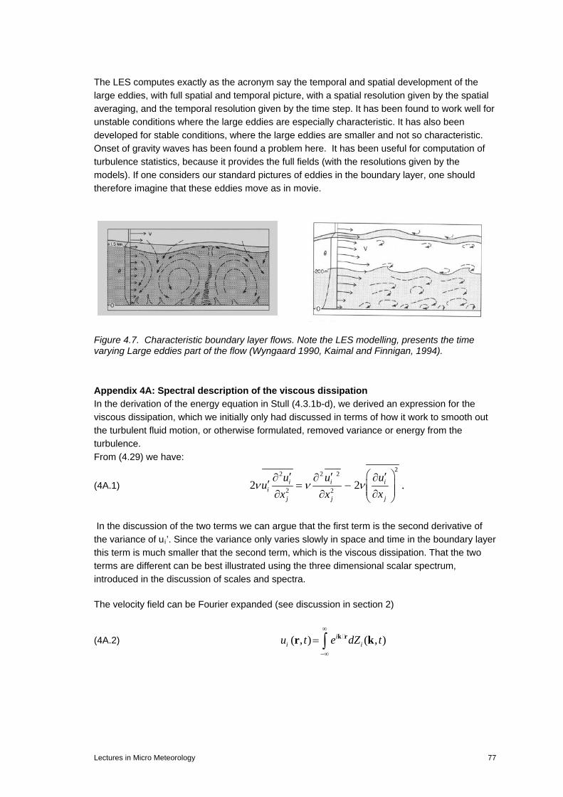
The LES computes exactly as the acronym say the temporal and spatial development of the large eddies, with full spatial and temporal picture, with a spatial resolution given by the spatial averaging, and the temporal resolution given by the time step. It has been found to work well for unstable conditions where the large eddies are especially characteristic. It has also been developed for stable conditions, where the large eddies are smaller and not so characteristic. Onset of gravity waves has been found a problem here. It has been useful for computation of turbulence statistics, because it provides the full fields (with the resolutions given by the models). If one considers our standard pictures of eddies in the boundary layer, one should therefore imagine that these eddies move as in movie. Figure 4.7. Characteristic boundary layer flows. Note the LES modelling, presents the time varying Large eddies part of the flow (Wyngaard 1990, Kaimal and Finnigan, 1994). Appendix 4A: Spectral description of the viscous dissipation In the derivation of the energy equation in Stull (4.3.1b-d), we derived an expression for the viscous dissipation, which we initially only had discussed in terms of how it work to smooth out the turbulent fluid motion, or otherwise formulated, removed variance or energy from the turbulence. From (4.29) we have:

(4A.1)

22 2 2

2 22 2 .i i ii

jj j

u u uu

xx xν ν ν

′ ′ ′∂ ∂ ∂′ = − ∂∂ ∂

In the discussion of the two terms we can argue that the first term is the second derivative of the variance of ui’. Since the variance only varies slowly in space and time in the boundary layer this term is much smaller that the second term, which is the viscous dissipation. That the two terms are different can be best illustrated using the three dimensional scalar spectrum, introduced in the discussion of scales and spectra. The velocity field can be Fourier expanded (see discussion in section 2)

(4A.2) ( , ) ( , )ii iu t e dZ t

∞

−∞

= ∫ k rr k


(4A.3) *( , ) ( , ) ( , )ij i jS t dZ t dZ t∞

−∞

′= ∫k k k

For the isotropic turbulence approximation we can define the scalar three-dimensional power spectrum, E(k), being only a function of the length of the wave number vector, k, not its orientation.

(4A.5) 2

( ) ( ) ,i i

ii

k k k

E k S d=

≡ ∫∫∫ k k

(4A.6) 2 2 21 2 3

0

1 1 ( ) ( )2 2i iu u u u u E k dk

∞

= + + = ∫

Hence in spectral form, the first right hand side element in (4.49) is:

(4A.7) 2 2 2

2 20

2 ( ) ;i

j j

uE k dk

x xν ν

∞′∂ ∂=

∂ ∂ ∫

which is just shows that this term is quite small because the variance changes little for homogeneous turbulence. To derive the second term we start by:

(4A.8) ( , ) ( , ).ii j i

j

u t ik e dZ tx

∞

−∞

∂=

∂ ∫ k rr k

From this follows:

(4A.9)

2 *

2 2

( ( , )) ( ( , )) ( ( , ))

( ) ( ) .

i ii j i j i

j

j ii

u t ik e dZ t ik e dZ tx

k S d k E k dk

ν ν

ν ν

∞ ∞−

−∞ −∞

∞ ∞

−∞ −∞

∂= −

∂

= =

∫ ∫

∫ ∫

k r k rr k k

k k

Relative to the variance, the viscous dissipation term is seen to have much less contributions from the small wave numbers and much larger contributions from the large wave number regions of the spectrum. We recall the description of the three wave number regions of E(k), from section 2.


Figure 4A.1. Schematic energy, or variance, spectrum for the atmospheric boundary layer, shown with the three characteristic spectral regions (Tennekes and Lumley,1972). We can separate the power spectrum into three regions as shown on the next figure, the production range, with k ∼1/Λ, where energy is extracted from the mean profile, a dissipation range, where the fluid motion is dissipated by viscosity, for k > η ∼ (ν3 / ε)1/4, which for typical atmospheric flows is about 1 mm. η is called the Kolmogorov dissipation scale and is a combination of viscosity and dissipation as seen. In between there is a region, where the spectrum depends only on the wave number and the dissipation. This region is called the inertial sub-range. Since the spectrum describes wind variance per wave-number increment, it has the dimension: m3/sec2. Dissipation is destruction of variance by viscosity; hence it has the dimension of variance per second, or m2/s3. Finally, for the inertial sub-range the spectrum for the dissipation looks like: (4A.10) 2 2 / 3 1/ 3( ) ( )k k E k kαε +Ε = =

To model the enhanced destruction of turbulence in the dissipation range for k>η, the inertial subrange form of (4.57) is multiplied by an exponential form that generally is represented as (e.g. Larsen and Højstrup,1982) (4A.11) 2 2/3 1/3 4/3( ) ( ) exp( ( ) )k k E k k n kαε η+Ε = = ⋅ − ,

which is the Kolmogorov dissipation spectrum with n being a constant of order one. A dissipation spectrum is plotted together with other spectra in Figure 2.22 It is obvious from this description that the dissipation takes mainly place at high wave numbers, which is in according with the here presented spectral picture. Also the discussion shows that that the second term in (A.1) is much larger and of completely different nature from the first term.


5. The Ekman boundary layers

For convenience we repeat the mean value equations:

(5.1)

3

*

12 ( );

1( )

( ) ;


j i j j

jj T j

j j j p jp

j q jj j j

du u u upu g u u u

dt t x x x x

Qd LEu k u

dt t x x x C xC

dq q q q Eu k u q

dt t x x x

δ ε η νρ

θ θ θ θθ

ρ ρ

ρ

∂ ∂ ∂∂ ∂ ′ ′= + = − − − Ω + −∂ ∂ ∂ ∂ ∂

∂∂ ∂ ∂ ∂ ′ ′= + = − − −∂ ∂ ∂ ∂ ∂

∂ ∂ ∂ ∂ ′ ′= + = − +∂ ∂ ∂ ∂

Neglecting molecular terms, radiation term and E-terms, we find for horizontally homogeneous stationary flow with zero vertical mean velocity.

(5.2)

2 1 31 3

1 2 32 3

1 2 2 1 3 33 3

3 33 3

.10 ( )

10 ( ).

10 2 ( ) .

:

0 ( ) ; 0 ( );

C

C

The three momentum equationsp f u u ux x

p f u u ux x

pg u u u ux x

The scalar equations

u u qx x

ρ

ρ

η ηρ

θ

∂ ∂ ′ ′= − + −∂ ∂∂ ∂ ′ ′= − − + −∂ ∂∂ ∂ ′ ′= − − − Ω − −∂ ∂

∂ ∂′ ′ ′ ′= − = −∂ ∂

For such simple conditions it is seen that the scalar fluxes are constant with height. At the top of the boundary layer the turbulence terms disappear, by definition, hence we see that the pressure terms and the Coriolis terms must balance, giving rise to the so called Geostrophic wind, given by:

(5.3) 1 22 1

1 1 1 1( , ) ( , ) ( , ) ( , ) ;G G g g

C C C C

p p p pG U U u v

f x f x f y f xρ ρ ρ ρ∂ ∂ ∂ ∂

= = = − = −∂ ∂ ∂ ∂

where it is indicated that we can use several notations for the same variable. See Figure 5.1.


Figure 5.1. Schematics of the Geostrophic balance between pressure gradient force and Coriolis force, denoted PGF and CF. We start considering only the two horizontal equations, which we can now write:

(5.4) 2 2 1 3

3

1 1 2 33

0 ( ) ( )

0 ( ) ( ).

C G

C G

f u U u ux

f u U u ux

∂ ′ ′= − −∂

∂ ′ ′= − − −∂

,

These two equations describe the so-called Ekman spiral wind profile. Derivation of the spiral: We have the two equations for the horizontal wind components.

(5.5) 2 2 1 3

3

1 1 2 33

0 ( ) ( )

0 ( ) ( ).

C G

C G

f u U u ux

f u U u ux

∂ ′ ′= − −∂

∂ ′ ′= − − −∂

Figure 5.2. Within the boundary layer the wind is seen as a balance between the pressure, the Coriolis and the frictional forces, denoted CF and F respectively.

So far, we have not considered the directions of the horizontal axes. We now fix them such that x1 is along the Geostrophic wind. Changing also to the (x,y,z) and (u,v,w) form for the variables, the equations take the form:


(5.6) 3

3

0 ( )

0 ( ) ( ).

C

C

f v u wx

f u G v wx

∂ ′ ′= −∂

∂ ′ ′= − − −∂

For simplicity, we now use a gradient diffusion for the turbulence terms, with constant diffusivity. In later sessions we shall consider more realistic closure schemes.:

(5.7)

2

2

2

2

( )

( ) ( ) .

C

C

u uf v u w K Kz z z z

v vf u G vw K Kz z z z

∂ ∂ ∂ ∂′ ′= = − =−∂ ∂ ∂ ∂

∂ ∂ ∂ ∂′− − = = − =−∂ ∂ ∂ ∂

Combining to the complex variable, and multiplying the second equation by i, we get:

(5.8) 2

2

2

2

;

( )

C

C

W u iv

uf v Kz

vif u G iKz

= +

∂=−

∂∂

− − = −∂

Adding the two last equations yields, since 1/(-i) = i:

(5.9) 2

2

1( ) ( ) ( )C C C CWK if u G f v if u v G if W G

iz∂

− = − − + = − + − = − −−∂

or:

(5.10) 2

2 ( ) 0 ,CWK if W Gz

∂− − =

∂

This is a simple second order differential equation with constant coefficients. Hence, the solution can be written:

(5.11) 12

exp((1 ) ) exp( (1 ) );

/ ; (2 / ) ;E E C

W G A i Z B i Z

Z z h h K f

− = + + − +

= =

where we have introduced the Ekman height scale, hE. The numerical value of the Coriolis parameter is interesting only if one wants to work on the Southern Hemisphere. The boundary conditions are: (5.12) 0 0; ;W for z W G for z= = → →∞

The last of these means that A = 0. The first then means that B = -G. Hence, the solution of W looks as: (5.13) (cos( ) sin( ) ).Z

CW G Ge Z i Z signf−− = − − Going back to the two components, we get:


(5.14) /

/

(1 cos( )) (1 cos( / ));

sin( ) sin( / ) .

E

E

z hZE

z hZE C

u G e Z G e z h

v Ge Z signf Ge z h signf

−−

−−

= − = −

= =

Since, in this coordinate system, u is along the Geostrophic wind, we can find the angle between the surface wind and the Geostrophic wind, θ.

(5.15) 0 0 0

( cos( ) sin( ))tan lim lim lim ;

cos( ) sin( )

Z ZC

CZ Zz z z

dve Z e Z signfv dz signf

duu e Z e Zdz

θ− −

− −→ → →

−= = = =

+

The result θ≈ 45° is not correct, for neutral homogeneous condition it is closer to 20°. But some results hold: Looking along the vectors, the surface wind is to the left of the Geostrophic wind, and further the angle is independent on the size of fC. Under all circumstances, it varies much with other conditions like stability, baroclinity and other types of heterogeneity. Below, we show a three dimensional diagram of the turning of Ekman spiral on the Northern Hemisphere. Figure 5.3. Ekman spiral on the Northern Hemisphere (Larsen and Jensen, 1983), showing the pressure gradient force, P, the frictional force, F, and the Coriolis force, C, from the top of the boundary layer and down towards the surface. Next we consider a number of special aspects of the above derivation. The turbulence diffusivity: Above the Ekman height, hE, was defined from the Coriolis parameter and the turbulence diffusivity. We know hE typically to be of the order of 500 meter in the atmosphere, hence we can deduce the magnitude of K.

(5.16) 1

2 4 4 2 12 1 1(2 / ) 25 10 1.410 15 .2 2E C C Eh K f or K f h m s− −= = ≈ ⋅ ⋅ ≈

Comparing with the corresponding kinematic molecular diffusivity, ν ≈ 1.5⋅10-5 m2 s-1, it seen that turbulence diffusion is about a million times more efficient than molecular diffusion for the same gradient. Therefore, it is often justified to neglect the molecular terms in the equations compared to the turbulence term. Compare the mean value equations for the boundary layer,


where neglect of the molecular parts of the flux divergence terms will almost always be justified by the comparison above. :

(5.17)

31 2 ( );

( ) ,

( ) ;


j i j j

j T jj j j p

j q jj j j


d LEu k udt t x x x C

dq q q q Eu k u qdt t x x x

δ ε η νρ

θ θ θ θ θρ

ρ

∂ ∂ ∂∂ ∂ ′ ′= + = − − − Ω + −∂ ∂ ∂ ∂ ∂

∂ ∂ ∂ ∂ ′ ′= + = − −∂ ∂ ∂ ∂

∂ ∂ ∂ ∂ ′ ′= + = − +∂ ∂ ∂ ∂

Surface characteristics of the Ekman layer Above we have seen that the u and v parts of the Ekman layer mean wind speed profiles converge toward same values for z→0. We shall now consider in more details the behaviour of the Ekman layer close to the surface. We start with the total stress:

(5.18) 1

2 2 2 2( ) ;xz yzuρ τ τ τ∗ ≡ = +

It is seen that the two components of the stress can be considered as vectors, attacking a horizontal plane along the x and y directions, respectively. This means that we can combine these two components as vectors. Note further, that we have introduced a scale velocity for the turbulence, u∗, denoted the friction velocity. The stress components are computed as:

(5.19) ; ;yzxz u vu w K v w Kz z

ττρ ρ

−− ∂ ∂′ ′ ′ ′= = − = = −∂ ∂

. We can now find the total surface stress as defined above, from the Ekman profile and the relations above. We use subscript 0 to denote values at the surface. :

(5.20) 1 1

22 2 2 22 2*0 0 0 00(( ) ( ) ) (( ) ( ) ) ,u vu u w v w K K

z z∂ ∂′ ′ ′ ′= − + − = +∂ ∂

The wind profiles were differentiated when we determined the angle between the Geostrophic wind and the surface wind (5.15). Using these results we get (5.21) 2

*0 / 2E Cu Gh f=

This shows the relation between the surface stress, the Geostrophic wind and characteristics of the Ekman profile, namely, fC and hE.


When studying the behaviour closest to the surface it is most convenient to rotate the coordinate system, such the x axis is along the surface mean wind, u, rather than along the Geostrophic wind. Again we have z, w being vertical and y, v being the horizontal component perpendicular to x, u.

Figure 5.4. Relation between coordinate systems aligned with the Geostrophic wind and with the surface wind. The general formulation for the Ekman spiral was:

(5.22) 0 ( ) ( )

0 ( ) ( )

C G

C G

f v V u wz

f u U v wz

∂ ′ ′= − −∂

∂ ′ ′= − − −∂

In the coordinate system with x along the mean wind, <v> =0, because u is aligned with the mean wind. Hence, the equation reduces generally to:

(5.23) ( ) ;

( ) ( );

C G

C G

u w f Vz

v w f u Uz

∂ ′ ′ = −∂∂ ′ ′ = − −∂

Integrating from z = 0 to z, we obtain:

(5.24) 0 0

00 0

( ) ( ) ( ) ;

( ) ( ) ( ( )) ( ( )) ,

z C G C G

z z

z C G C G

u w u w f V z u w f V z

v w v w f U u z dz f U u z dz

′ ′ ′ ′ ′ ′= − = +

′ ′ ′ ′ ′ ′ ′ ′= + − ≈ −∫ ∫

where we have introduced that fCVG is negative in this coordinate system and that the v-w cross covariance is close to zero at the surface. This equation is rather general without closure assumptions etc. In the surface wind system, we would expect that at the surface all the surface stress was along the mean wind carried by the u-w-cross-co-variance, which would then equal u2

∗o, while the v-w-cross-co-variance would be vary close to zero close to the ground. We can check if this is consistent with the Ekman solution, by turning the coordinate system, as given in the figure above. We get:

θ

x G

y G x

s

y s

-

Ekman Spirall

(5.25)

cos sin ;

cos sin .

.4

s g g

s g g

u u vv v u

θ θ

θ θ

πθ

= +

= −

≈

where, we denote the wind in the surface system by subscript s and the wind in the Geostrophic system by subscript g. From the Ekman spiral equations we now get:

(5.26)

2*0

( cos sin )

(cos ( cos( ) sin( )) sin (( cos( ) sin( )))

1 2 (2( cos( )) / 2 0.2 2

( cos sin )

ss g g

Z Z Z Z

E

ZC E C E

ss g g

E

du du dvu w K K Kdz dz dz

KG e Z e Z e Z e Zh

f h G e Z f h G u for z

similarlydv dv duv w K K Kdz dz dz

KGh

θ θ

θ θ

θ θ

− − − −

−

′ ′ = − = − + =

= − + + − =

= − → − = − →

′ ′ = − = − − =

= − (cos ( cos( ) sin( )) sin (( cos( ) sin( )))

1 2 (2( sin( )) 0 0.2 2

Z Z Z Z

ZC E

e Z e Z e Z e Z

f h G e Z for z

θ θ− − − −

−

− − + =

= → →

Where, we have utilized the variable Z = z/hE, and also used the results from above relating the Ekman height and the diffusivity, K. The sign of the Coriolis parameter is neglected here. It is seen that in the surface wind also the Ekman solution yields that the total surface stress is carried by the u-w cross-co-variance, while the v-w-cross co-variance at the ground is zero. We notice that the earlier introduced surface stress scale, u∗o, equals (-<u´w´>)o½ in this coordinate system. By first order expansion, the equations for the surface stress can now be written in terms of height variation for u∗. This makes it somewhat easier to evaluate the importance of the height variation, because we can now consider the relative variation of u∗/u∗o :

(5.27)

2 20

2

2 22 2

0 0

( ) ( ) ; : u u ;

u u (1 ) u (1 ) u (1 );2u 22

( ) ( ')( ) u ( ) u (1 )u u

z C G z o C G

C G Gz o o o

o EEz z

Gz o C o

o o G E

u w u w f V z or f V zor

f V z V z zhGh

U u z u z dzv w f dzU h

∗ ∗

∗ ∗ ∗ ∗∗

∗ ∗∗ ∗

′ ′ ′ ′= + − = − +

≈ − ≈ − ≈ −

′ ′′ ′ ′= − = −∫ ∫

In the equation for u∗, we have gradually introduced approximations from the Ekman spiral, first through the expression for the total surface stress, second assuming θ ≈ 45°. For z/hE less than about 20% we see that u∗ is within 10% of u∗o and it reduces approximately linearly. In the same z- interval <v’w’> increases from about zero and up slightly slower than proportionally to z/hE. We can further see that although the stress may vary across the layer, the surface value u∗o will characterize not only the magnitude but also the changes across the layer, and the changes will be small relative to u∗o. This layer closest to the surface is called the surface layer. It is characterized by that all fluxes can be considered constant with height, since we saw in the beginning of this section that the scalar fluxes were independent of height. Although we have used the simple Ekman spiral somewhat to derive this conclusion, we can also see that the existence of the surface layer is more general than the Ekman solution for the whole boundary layer. We shall return quite intensively to this layer. In the coordinate system with the surface wind along the x-axis, the Ekman spiral looks as seen below. Notice, the height of the boundary layer has been approximated by u∗o /fC. Figure 5.5. The Ekman spiral seen in a coordinate system aligned with the surface mean wind. Notice that the boundary that z is normalized with u∗/fc rather than hE. Ocean current Ekman spiral. Before leaving the Ekman layers, we shall see how an atmospheric Ekman layer above an ocean surface drives and ocean Ekman layer below, since this was really the way it was first derive by Ekman in 1905, confirming observations of drifting ice by Nansen a few years earlier, In the ocean we can neglect the Geostrophic wind from the equation, which then looks like:

(5.28) 0 ( )

0 ( )

C

C

f v u wz

f u v wz

∂ ′ ′= −∂∂ ′ ′= − −∂

Notice, we keep the same direction of the z-axis. Ocean depths is then for z→-∞. The equation is reformulated with diffusivity, which we for water give the subscript w, Kw .

(5.29)

2

2

2

2

0

0 ;

C w

C w

uf v Kzvf u K

z

∂= +

∂∂

= −∂

As for air we define a complex variable, W, and as for the air we derive the equation to be:

(5.30) 2

2

;

0.C

w

W u ivifW WKz

≡ +

∂− =

∂

Following the procedure from the atmosphere we have:

(5.31) 12

exp((1 ) ) exp( (1 ) );

/ ; (2 / ) ;Ew Ew w C

W A i Z B i Z

Z z h h K f

= + + − +

= =

where the water Ekman depth has got a subscript w, like the diffusivity. Since, W→0 for z→-∞, it follows that B=0. We can now write the component equations from W.

(5.32)

( ) ( sin );

( sin );

( sin );

Zr i

Zr i

Zi r

W A iA e cosZ i Z

u e A cosZ A Z

v e A cosZ A Z

= + +

= −

= +

The boundary conditions at the water surface derive from continuity of stress at the surface. We formulate the stress continuity as:

(5.33) 0 0

0 0

1 ;21 ,2

w w a a a E C

w w a a a E C

u uK K Gh fz zv vK K Gh fz z

ρ ρ ρ

ρ ρ ρ

∂ ∂= =

∂ ∂

∂ ∂= =

∂ ∂

where the surface stress values on the atmospheric side was derived earlier. Differentiating on the ocean side we get.

(5.34)

1 ( sin )

( sin ) ( sin cos )

1 ( ) 0,

Zr i

EZ

r i r iE

r iE

u u Z e A cosZ A Zz Z z h Z

e A coZ A Z A Z A Zh

A A for Z and similar for vh

∂ ∂ ∂ ∂= ⋅ = − =

∂ ∂ ∂ ∂

− + − −

→ − →


(5.35) 0

0

1( ) ;21( ) ,2

ww w w r i a E C

Ew

ww w w r i a E C

Ew

KuK A A Gh fz h

KvK A A Gh fz h

ρ ρ ρ

ρ ρ ρ

∂= − =

∂

∂= + =

∂

This solves to:

(5.36) 2

0;1 12 2 ;

12

i

a E C a E Ca E

rw w Ew

c EwwEw w

Ew

A

Gh f Gh f hA G

K hf hh

h

ρ ρ ρρρ

ρ

=

= = =

where we have used expressed Kw in terms of hE and fC. Hence, we arrive at:

(5.37)

/

/

( ) cos( / ),

( ) sin( / );

Ew

Ew

z ha EEw

w Ew

z ha EEw

w Ew

hu z Ge z h

hh

v z Ge z hh

ρρρρ

=

=

First of all the equation shows that the surface current runs along the Geostrophic wind, not the surface wind or for that matter the surface stress. It was to explain observations of ice floe indicating something like that, that Ekman did his derivation. As the depth increase the current veers toward right. Notice, that we have to derive hEw from other considerations, or for that matter Kw, just as we in the atmosphere used observations for hE. We would expect the depth of the Ekman layer to be associated with the strength of the turbulence mixing. Due to the stress continuity over the surface we have that u∗w ≈u∗a(ρa/ρw)½ . Taking u∗ as indicator of the turbulence strength we would assume that a similar ratio would relate hEw and hE, and that hEw ≈hE(ρa/ρw)½, which is approximately true. Then we further see that the surface current relates to the Geostrophic wind through the same ratio, being roughly 1/30. The following figure illustrates the characteristics of the two Ekman spirals. Here one could also notice that the surface stress in the atmosphere is along the surface wind. The surface stress at the ocean surface is 45º of the surface current.


Figure 5.7. Coupled ocean atmosphere Ekman spirals (Stull, 1991) Appendix 5A. The Baroclinic Boundary Layer and the Thermal Wind. The picture of the boundary layer can be modified by many kinds of heterogeneity and improved parameterizations. A simple modification arises when one considers the importance of horizontal temperature gradients, as will often be present in reality. So far, we have only allowed for horizontal gradients of pressure to drive the flow. To feed in the information about the changing horizontal temperature, we use the so-far unused equation for the vertical component.

(5A.1) 1 2 2 1 3 33 3

10 2 ( )pg u u u ux x

η ηρ∂ ∂ ′ ′= − − − Ω − −∂ ∂

Differentiating this with respect to the horizontal coordinates, i = 1,2 we obtain.

(5A.2) 1 2 2 1 3 33 3 3

1 10 ( 2 ( ) ) .i i

p pg u u u ux x x x x

η ηρ ρ

∂ ∂ ∂ ∂ ∂′ ′= − − − Ω − − = −∂ ∂ ∂ ∂ ∂

Assume now that ρ varies horizontally due to the horizontal temperature variation. Differentiating by parts, we get:


(5A.3)

3 3 3

23

3 3

3

1 1 1

( ) 1 1

1 1 1

1 1 10;

i i i

i i

i i i

i i i

p p px x x x x x

g px x x

g T p pT x x x x x

g T p pT x x x H x

ρ ρ ρ

ρ ρρ

ρ ρ ρ

ρρ ρ ρ

ρ ρ

∂ ∂ ∂ ∂ ∂ ∂= + =

∂ ∂ ∂ ∂ ∂ ∂

− ∂ ∂ ∂= + =

− ∂ ∂ ∂

∂ ∂ ∂ ∂ ∂= − + + ⋅ ⋅ =

∂ ∂ ∂ ∂ ∂

∂ ∂ ∂ ∂= − + − =

∂ ∂ ∂ ∂

where, first we have used the hydrostatic equation in the first term and reversed the order of differentiation in the second term. The horizontal variation of ρ is assumed dominated by the temperature variation as usual. Thereafter, we have multiplied and divided by ρ in the second term and differentiated by parts, and finally used the hydrostatic balance again, introducing the scale height of the atmosphere, H. Now expressing the horizontal pressure gradients as the Geostrophic wind components, we obtain, for i = 1, 2:

(5A.4) 2 2

3 1

1 23 2

1( ) ,

1( ) ;

C G C G

C G C G

g Tf U f U

x H T x

g Tf U f U

x H T x

∂ ∂− =

∂ ∂

∂ ∂− + =

∂ ∂

We will here neglect the second term, because we at most integrate to the Ekman- hE, being of the order of 3-5% of the scale height. Hence, we can derive a vertically varying Geostrophic wind due to a horizontal temperature gradient:

(5A.5) 1 1 0 3 1 0 2 32

2 2 0 3 2 0 1 31

,

;

,

G G GC

G G GC

g TU U x U A xf T x

g TU U x U A xf T x

∂≈ − ⋅ = − ⋅

∂

∂≈ + ⋅ = + ⋅

∂

where the integration constants are the surface Geostrophic wind. One can now insert these expressions for the Geostrophic winds into the expression for the Ekman spiral equations.

(5A.6)

1

2

2

2 2 0 1 3 23

2

1 1 0 2 3 23

0 ( )

0 ( ) .

C G

C G

uf u U A x Kx

uf u U A x Kx

∂= − − −

∂

∂= − − + +

∂


Solutions are show on the next figure, where the arrows show different baroclinic forcing. In the solutions presented the x1 axis is placed along the unperturbed Geostrophic wind.

Figure 5A.1 Behavior of the Ekman spiral for four examples of baroclinic forcing all with the same magnitude, indicated with the unit-length arrow. The direction of the arrow refers to the sign of the A1 and A2 terms in the definition of the thermal wind that is to the signs of the two horizontal temperature derivatives in the definition of the A-terms. . From the top to the bottom the sign of the forcing is: (A1, A2) = (0,-1 ), (0, +1), (+1, 0), (-1,0). We note that the modification of the Geostrophic wind, and thereby also the wind itself, is largest at the top. Comparing with the definition the resulting change is seen to be qualitative reasonable. For example, in the lowest figure A1 = -1 and A2 = 0, meaning that we must expect little or no changes in u1, while U2G and u2 will be modified in negative direction (NO Jensen, personal communication).


All examples have the same strength of baroclinic forcing, but the direction of the arrows shows the sign of A-terms of the corrections. Vertical arrows, means only A2 (A2 reflect the horizontal temperature gradient in the x2 direction) is different from zero, with sign given by the direction of the arrow, similarly for horizontal arrows. In the figure we have chosen the magnitude of the two A-terms to be A≈ 0.015 m/s/m, corresponding to a horizontal temperature gradient of about 0,05 °C/km. From the figure, we can conclude that the shape of spiral is indeed sensitive to the thermal wind. However, we see as well that the angle between the Geostrophic wind and the surface wind shows little sensitivity to this kind of forcing. This concludes our discussion of the atmospheric Ekman boundary layer. For a horizontally homogeneous stationary boundary layer, we have seen that use of constant turbulence diffusivity allow us to derive the so-called Ekman spiral solution for the variation of the mean wind with height. We have estimated the diffusivity needed to be in according with data and found it to be about one million times larger than its molecular brother, the cinematic viscosity. We have been able to include horizontal variation of the mean temperature and found that this does modify the form of the Ekman spiral considerably. Indeed, although the Ekman spiral is found in the data, it is found comparatively rarely, indicating that boundary layers, simple enough to justify the used simplifications, are somewhat rare. As expected the assumption of a constant K-value is too simple, as we will see a height dependent K fits better the data. Also thermal stability can be built in to K. Now however, the equations have to be solved numerically. Notice, that in our solution of the Ekman spiral, we have not avoided the closure problem. We have had to specify K from other information than what is in the mean value equations themselves. We use information about the hE, the Ekman height, which was based on measurements. Finally we have identified a surface layer within the 20-100 meters closest to the surface. In this layer one could with good approximation assume that all fluxes were constant with height.


6. The atmospheric surface boundary layer. Monin-Obuchov scaling

In the discussion of the Ekman layer, we have seen that the lowest part of the layer is characterised by having fluxes that varies little or not at all with height. This means that for horizontally homogeneous stationary flow, the lowest part of the boundary can be characterized using the surface fluxes plus maybe a few more variables. The use of dimensional analysis and normalising variables with characteristic parameters has and long record within fluid dynamics. It generally involves some guesswork as to what are the important parameters, some experimental data to use as guidance and some theory as to how one should go about it, and finally and very important experimental validation of the derived formulations. In the earlier chapters, we have seen simple dimensional analysis, when the turbulence diffusivities were established, as being product of a characteristic velocity parameter and a characteristic length- scale. (6.1) ,K vα≈ where v is the relevant velocity scale, is a relevant length scale, and α is a dimensionless numerical constant, which should be of order one, if the most relevant characteristic parameters have been chosen. As we found for the turbulence diffusivities, there will often be several different sets of possible characteristic parameters. The experimental verification is very important. The aim of the following analysis is to describe as well as possible the mean values, their vertical gradients, and the turbulence characteristics for a stationary horizontally homogeneous atmospheric surface boundary layer. Such a surface boundary layer can be said to be the simplest non-trivial boundary layer one can imagine. We shall use the equations for mean values and the turbulence variance to map the problem. A general version of the mean value equations was written on our way to the Ekman spiral.


(6.2)

2 1 31 3

1 2 32 3

1 2 2 1 3 33 3

33

33

.10 ( )

10 ( ).

10 2 ( ) .

:

0 ( )

0 ( );

C

C

The three momentum equationsp f u u ux x

p f u u ux x

pg u u u ux x


ux

u qx

ρ

ρ

η ηρ

θ

∂ ∂ ′ ′= − + −∂ ∂∂ ∂ ′ ′= − − + −∂ ∂∂ ∂ ′ ′= − − − Ω − −∂ ∂

∂ ′ ′= −∂∂ ′ ′= −∂

Introducing the geostrophic wind and turning the coordinate system along the surface mean wind, and changing to x,y,z coordinates we obtain:

(6.3) 2

.

( ) ;

( ) ( );.

10 2

:

0 ( )

0 ( );

C G

C G

y

The three momentum equations

u w f Vz

v w f u Uz

pg u wz z


wz

wqz

ηρ

θ

∂ ′ ′ = −∂∂ ′ ′ = − −∂

∂ ∂ ′= − − + Ω −∂ ∂

∂ ′ ′= −∂∂ ′= −∂

We can use the first two of these equations to derive the rate of change of the surface stress with height, using the result to define the surface layer, as the layer through which the surface stress did not change too much with height, through the following equation (remember VG is negative when fc is positive).


(6.4)

2 20

2

2 22 2

0 0

2

( ) ( ) ; : u u ;

u u (1 ) u (1 ) u (1 );2u 22

( ) ( )( ) u ( ) u (1 ) ;u u

u u ( ) / u 0 1.

z C G z o C G

C G Gz o o o

o EEz z

Gz o C o

o o G E

z o z oE

u w u w f V z or f V zor

f V z V z zhGh

U u z u z dzv w f dzU h

orzand v w for

h

∗ ∗

∗ ∗ ∗ ∗∗

∗ ∗∗ ∗

∗ ∗ ∗

′ ′ ′ ′= + − = − +

≈ − ≈ − ≈ −

′ ′ ′′ ′ ′≈ − = −

′ ′≈ ≈ <<

∫ ∫

In the last part of (6.4) we have used the results and notation from section 5 about the Ekman spiral, thr Ekman height, hE, and the friction velocity, u∗., and that it close to the surface changes slowly with height from its surface value, u∗o. Other fluxes of importance are <w’θ’> and <w’q’> that control the fluxes of heat and humidity through the layer. As we have specified the layer, we have <v > = 0, hence the Coriolis parameter is unlikely to be important, because it controls the cross talk between the equations for the two horizontal velocities. From the equations, it looks, as the Coriolis parameter is important only for the rate of change of the stress through the surface layer. There is no obvious use of the equation for the mean vertical velocity, since we have assumed that to be zero. All considered we find little additional use for the mean value equations for our (strongly) simplified surface layer flow. We now proceed to the variance equations derived in our effort to evaluate the different closure possibilities for the equations in Micro Scale Meteorology 4. We use the notation: e= u’i2, as the total fluctuating turbulence variance. The general equations look as follows, from section 4.

(6.5)

3

22 2

22 2

( ) ( )( )1 1 1 1 ;2 2 2

( )1 1 12 2 2

( )1 1 12 2 2

j jv ij i j

j j j jv

jj j

j j j

jj j q

j j j

u e u pg u ue eu u ut x x x x

uu u

t x x x

u qq q qu q ut x x x

θ

θε

ρθ

θθ θ θθ ε

ε

′ ′ ′∂ ∂′ ′ ∂∂ ∂ ′ ′+ = − − − −∂ ∂ ∂ ∂ ∂

′ ′∂′ ′∂ ∂ ∂′ ′+ = − − −∂ ∂ ∂ ∂

′ ′∂′ ′∂ ∂ ∂′ ′+ = − − −∂ ∂ ∂ ∂

We now impose the stationarity and horizontal homogeneity demands of our simplified surface layer, and turn the coordinate system along the mean surface wind.

(6.6)

2 2

2 2

( )1 1 ( ) 1 ( )0 ;2 2

1 1 ( )02 21 1 ( )02 2

v

v

q

t p

g wde u w e w pu wdt z z z

d wwdt z z

dq q w qq wdt z z

B P T T D

θ

θε

ρθ

θ θ θθ ε

ε

′ ′ ′ ′ ′∂ ∂ ∂′ ′= = − − − −∂ ∂ ∂

′ ′ ′∂ ∂′ ′= = − − −∂ ∂

′ ′ ′∂ ∂′ ′= = − − −∂ ∂

The budget equations for the turbulence variance as derived in section 4. They are here simplified to the conditions in a simple stationary horizontally homogeneous surface boundary layer.

The terms are denoted: B for Buoyancy, P for Production, Tt for flux divergence of turbulence flux of variance, Tp for flux divergence of pressure induced transport of variance, and D for Dissipation. Also for these equations we note that the Coriolis parameter does not enter, meaning that it is unimportant for our problem. However, the equations include relations between many profile quantities and turbulence quantities. We shall now show examples on how the dimensional analysis can be used to relate the different quantities to each other for simple subsets of the equations above. First, we will consider only the velocity profile without temperature effects. If we neglect most of the terms in the first equation it takes the form:

(6.7a) 2* 0uu

zε∂

− =∂

The dissipation just follows the local energy production in the first term. The equation underlines also the interaction between u∗ and the velocity profile. Hence it argues for that u∗ should be the velocity scale for the gradient. The profile must obviously also depend on z. Assuming that the wind profiles depends only on u* and z, we can normalise (6.7a) to obtain:

(6.7b) 3* *

1z u zu z u

εκ

∂= =

∂,

where κ is a dimensionless universal constant called the v Karman constant. It is a universal constant, because it can only depend on u* and z from our assumption, and no dimensionless argument can be made from these two variables. κ is experimentally found to be around 0.4. It is seen that a consequence of (6.7b) is that the wind speed varies logarithmically with the height, z.

(6.7c) 0 0( ) ln( / ),uu z u z zκ∗− = ⋅


Where the roughness length is introduced as an integration constant, and as the height where the wind speed becomes equal to 0u . At the surface we normally take 0u ~0.

To formulate this derivation in more formal way, one can use the dimensional analysis, denoted Buckinhams Pi theorem, described by Jensen and Busch (1982) in the appendix. Finally, we can refer to that the resulting logarithmic behaviour of the wind above the surface is one of the oldest and best established results from wind tunnels, where it is denoted the “ law of the wall”. Also for the near surface atmosphere, the logarithmic behaviour of wind profiles is well known. Having found a solution to the wind profile, we can now consider how the 3 variance equations will behave when being normalised by proper parameters. From the first results above, the constants and parameters in the equations we define the following characteristic parameters to make the terms non-dimensional. Notice, we obviously need a humidity scale and a temperature scale, since we include both temperature and humidity equations.

(6.8) 2* * * * * * *; ; ; ;/ ; ;

v vu u w u w u w u q q wg z

θ θ θ θ

θ

′ ′ ′ ′ ′ ′ ′ ′≡− ≡ − ≡ − ≡ −

Note that θv enters only in the Buoyancy term. We have converted the humidity flux and the temperature flux to a water vapour and a temperature scale, using u∗. The minus sign has a rational explanation for u∗ (that the momentum transport is downwards), for the other parameters the reason is just historical, and to make the production terms positive. We can now make the variance equations non-dimensional, using the parameters above.

(6.9a)

3

2 2

2

2 2

2

( )1 1 ( ) 1 ( )0 ;2 2

1 1 ( )0 ,2 2

1 1 ( )0 ,2 2

v

v

q

t p

g wde u w e w p kzu wdt z z z u

d w kzwdt z z u

dq q w q kzq wdt z z u q

B P T T D

θ

θε

ρθ

θ θ θθ εθ

ε

∗

∗ ∗

∗ ∗

′ ′ ′ ′ ′∂ ∂ ∂′ ′= = − − − − ⊗∂ ∂ ∂

′ ′ ′∂ ∂′ ′= = − − − ⊗∂ ∂

′ ′ ′∂ ∂′ ′= = − − − ⊗∂ ∂

Multiplication of the equations above by the factors at the right hand side makes all terms in the equations non-dimensional. Note, we have followed traditions by including the non-dimensional von Karman constant, k in the normalisation group. We write the resulting equations as:


(6.9b)

3

2

2

2

2

10 ( ) ( ) ( ) ( );

2 ( ) ( )

10 ( ) ( ) ( ),

2 ( )

10 ( ) ( ) ( ),

2 ( )

m Tt Tp

T

q Tq q

t p

kz de z z z z z z zz zu dt L L L L L L LL L

kz d z z z zzu dt L L L LL

kz d q z z z zzu q dt L L L LL

B P T T D

ε

θ θ εθ

ε

ϕ ϕ ϕ ϕ

θϕ ϕ ϕ

θ

ϕ ϕ ϕ

∗

∗ ∗

∗ ∗

∂ ∂= = − + − − −

∂ ∂

′ ∂= = − −

∂

′ ∂= = − −

∂

Below the individual functions are derived and discussed. The buoyancy term B, z/L, where L is the so-called Monin-Obuchov stability length scale:

(6.10) 3 3 2

( ) z z =L

( )

v

v v v

vv

g wkz zu u u

kg kgw

θθ θ θ

θθ∗ ∗ ∗

∗

′ ′= ≡ − −

′ ′

It is seen that L→ ±∞ for neutral condition, meaning for vanishing heat flux. Neutral conditions then means that z/L = 0. L is negative for unstable conditions and positive for stable conditions. The production terms, P, are derived as:

(6.11)

3

2

2

( ) ( ) ;

( ) ( )

( ) ( )

m

q

z kz u kz uu wL z u zu

z kz kzwL z zuz kz q kz qq wL z q zu q

θ

ϕ

θ θϕ θθθ

ϕ

∗∗

∗∗ ∗

∗∗ ∗

∂ ∂′ ′= − =∂ ∂

∂ ∂′ ′= − =∂ ∂

∂ ∂′ ′= − =∂ ∂ ,

where we assume that v. Karman's constant is the same for all variables. The flux divergence for turbulence transport of variance, Tt:


(6.12)

3 3

2 2

2 2

2 2

2 2

1 ( ) ( ) ( ) ;2 2 ( )

1 ( ) ( ) ( ) ;2 2 ( )

1 ( ) ( ) ( ) ;2 2 ( )

: ;( )

Tt

T

Tq

kz w e k w e z zz zu z z u L LL

kz w k w z zz zu z z u L LL

kz w q k w q z zz zu q z z u q L LL

zNote z zz LL

θ

ϕ

θ θ ϕθ θ

ϕ

∗ ∗

∗ ∗ ∗ ∗

∗ ∗ ∗ ∗

′ ′∂ ∂ ∂= ≡

∂ ∂ ∂

′ ′ ′ ′∂ ∂ ∂= ≡

∂ ∂ ∂

′ ′ ′ ′∂ ∂ ∂= ≡

∂ ∂ ∂

∂ ∂=

∂ ∂

The divergence of the pressure transport term, Tp, is done similarly:

(6.13) 3 3

1 ( ) ( ) ( ) ;2 2 ( )

Tpkz w p k w p z zz

zz z L Lu uL

ϕ∗ ∗

′ ′ ′ ′∂ ∂ ∂= ≡

∂ ∂ ∂

Finally the dissipation terms, D:

(6.14) 3 2 2( ) ; ( ) ; ( ) ;qq

kzkzz kz z zL L Lu u u q

θε εθ ε

εεεϕ ϕ ϕθ∗ ∗ ∗ ∗ ∗

= = =

Optimistically, we have written all the ϕ- functions as function of z/L and only z/L. How reliable is this? In the appendix, the dimension analysis above has been carried out for ϕm(z/L) based on the momentum equation, where the flux divergence terms have been neglected. Therefore, we would expect also the similar analysis to hold for ϕh(z/L) and ϕq(z/L), and therefore also for all the dissipation terms. Additionally, we see that z/L is the only free variable in the momentum equation, indicating that at least other types dependencies in the ϕ- functions must cancel, when these functions are added as prescribed by the equation or at least be of less importance. However there are indications that the flux divergence terms do depend also on other parameters (Elliot, 1972), mainly the boundary layer height, so that the M.O. scaling can be considered an approximation only, although a fairly good approximation. This is underlined also from the fact that the v Karman constant, a constant within the framework of the Monin-Obuchov similarity, empirically seems to show a tendency towards a week dependency on external parameters, like the surface roughness number, z0u∗ /ν (Larsen, 1993), but the statistics is uncertain. Under all circumstances, we noted above that the results of a dimensional analysis must be considered like a hint about where to look, rather than a truth derived from first principle, and experimental validation will always be necessary. An approach based on the Buckinhams PI theorem for dimensional analysis of the surface layer turbulence is presented in Jensen & Busch (1982), see appendix 6A. Here is illustrated that it is sometime successful in explaining the experimental data, sometime not. The later result is usually taken as indication of that one has somehow guessed wrongly for the important variables. Not all ϕ- functions have been equally well studied. Most comprehensive work has been conducted on the mean-profile expressions, followed by the dissipation terms. The flux


divergence terms have been relatively little studied, especially the one involving pressure, mostly because of the large difficulties in measuring the pressure fluctuations properly. In a following section, we shall see that the Monin-Obuchov scaled surface layer is but one scaling region in the atmospheric boundary layer. It can be considered correct in an asymptotic way when the influence of the other scales have vanished. Until then we shall just consider it an useful approximation. The experimental campaigns started in the middle of the 1960, where one got instruments that could resolve all of the three velocity components, the so-called sonic anemometer thermometer. The next figure 6.1 shows the set-up of the first of these. The setup on the figure shows how one could measure the mean temperatures and velocity gradient. The sonics provided fluxes and turbulence variances. Additionally, fast response hot-wire anemometers could provide the wind dissipation. Also other instruments were operated as seen on the figure. As seen the sonics operated at three levels, meaning the assumption of constant flux with height could be validated. Further it was possible to estimate many of the ϕ- functions at 3 levels, ϕm(z/L), ϕh(z/L), ϕε(z/L), and ϕTt(z/L). By plotting these functions versus z/L it was possible to evaluate if the functions could be considered function of z/L only, or they stratified according to the different measuring heights. Humidity was not measured. Also variances and spectra were evaluated as function of z/L. Basically, the Monin-Obuchov similarity was found to provide good approximations for these data and data from subsequent experiment. The following two figures show data from such experiments, this time conducted in Sweden.

Figure 6.1. Diagram of the experimental set-up during the Kansas 1968 surface layer experiment (Izumi, 1971). The first comprehensive experimental test of the Monin-Obuchov similarity hypotheses (Bush et al, 1973, drawing:C. Kaimal personal communication).


We shall now proceed to discuss details and consequences of some of the M.O. formulations.: The stability The stability is described by the parameter combination: z/L, with z/L = 0 denoting neutral. From the definition of L it is seen that it is a measure of the relative strength of the impacts on the turbulence from the dynamic part, through u∗, and from the thermal part through θ∗. The fact that all the stability is described by the ratio between z and L means however that stability is both a function of the relative strength between the thermal and the dynamic forces in the atmosphere and of the measuring height, meaning that irrespective of the overall atmospheric conditions, close to the ground the stability is neutral. Profile Expressions. We shall now consider the forms for the mean profile for ϕm(z/L), ϕθ(z/L), ϕq(z/L). The three functions all looks pretty similar. The typical form is illustrated on the figure below. The functional forms of the ϕ- functions can be summarised (Panofsky and Dutton, 1989, Högström, 1990):

(6.15) ( 0) 1 5 ; ( 0) (1 )

1 1: , 15. , : , 104 2

n

m q

z z z zL L L L

n nθ

ϕ ϕ α

ϕ α ϕ ϕ α

−> ≈ + < ≈ −

≈ ≈ ≈ ≈

Figure 6.2. Characteristic behaviour of the profile functions within the Monin-Obuchov surface layer similarity. The expression for the dissipation functions do qualitatively follow the production functions (ϕm–z/L), ϕθ(z/L) and ϕq(z/L), as indeed they must if the flux divergence terms in the equations are small. However, the exact match is debated, see next figure, where estimates of all functions are shown for the momentum balance is shown.

ϕ (z/L)

z/L

z/L

1,0

Figure 6.3. Experimentally determined Monin –Obuchov similarity functions from Högström (1990) as functions of (z-d)/L, where d is the zero level for z, called the displacement height, see section 7.The terms, P,B, Tp,Tt, and D are defined in Equation 6.9.The top figure shows unstable values, while the lower figure shows stable values.


From the ϕ- functions above, we can calculate the profile expressions. As example we chose the profiles of wind and potential temperature.

(6.16) 0 0

0 0 0

0

( )

1 ( )1( ) ( ) ;

( )

1 ( )1( ) ( ) ;T T

m

u z z m

mz z

z z

z z

z kz uL u z

zu uz Ldu dz dzkz L k z z

similarly

z kzL z

zz Ld dz dz

kz L k z z

θ

θ θ

θθ

ϕ

ϕϕ

θϕθ

ϕθ θθ ϕ

∗

∗ ∗

∗

∗ ∗

∂= ⇒

∂′

−′′ ′= = −

′ ′ ′

∂= ⇒

∂′

−′′ ′= = −

′ ′ ′

∫ ∫ ∫

∫ ∫ ∫

We use that u(z0) = 0, and θ(z0T) = θ0, that is some estimate of the surface temperature, and ϕm(z/L= 0) = ϕh(z/L= 0) = 1. This is really how the v. Karman constant has been chosen. Hence we get:

(6.17)

0

0

0

0

( ) ( ln( ) ( ) ( ))

1 ( )( ) ( ) ( )

z m

z

zu z zu z withk z L L

zzz L dz

L L z

ψ ψ

ϕψ ψ

∗= − +

′−

′− =′∫

and

(6.18)

0

00

0

0

( ) ( ln( ) ( ) ( ))

1 ( )( ) ( ) ( )

T

T

T

zT

z

zz zz withk z L L

zzz L dz

L L z

θ θ

θ

θ θ

θθ θ ψ ψ

ϕψ ψ

∗− = − +

′−

′− =′∫

For unstable condition the ψ - functions are complicated and positive, see e.g. Stull(1991), while for stable conditions the integration is trivial:

(6.19) ( ) ( ) 5z z zL L Lθψ ψ= = −

The values of ψ for z0/ L and z0T /L are often neglected, and ψ(0) = 0. We are now able to show the principal behaviour of the profiles for stable, neutral and unstable conditions. It should be pointed out that the temperature gradient and the θ∗ changes sign together.


The qualitative behaviour of the profiles are shown on the next figure, and it is clear how these functions do describe the lowest part of the characteristic profiles throughout the boundary layer as shown earlier

Figure 6.4.Characteristic profiles for the surface boundary layer for stable, neutral and unstable conditions. .

Figure 6.5 Typical boundary layer profiles of wind speed, U, temperature, T, and water vapour mixing ratio, q: a)Daytime unstable conditions. Part of the profiles is well mixed, i.e. no height variation. b) Night time stable conditions. Stronger height variation of profiles. c) Thermally neutral conditions. The profiles are logarithmic in a height interval.

( )u z

0( )zθ θθ∗

−

Ln(z)

Ln(z0) or

Ln(z0T)

z/L = 0,

z/L > 0

z/L< 0

Some aspects of the surface layer.

The Richardson number, Ri, is used throughout fluid dynamics to characterise the thermal stability of a fluid and the influence of thermal properties on the turbulence. There are two different Richardson numbers, the flux Richardson number, defined from gradients and fluxes, and the gradient Richardson number, defined from the ratio between the temperature gradient and the wind speed gradient.

We start our story with the simplified energy equation used earlier:

(6.20)

( )1 1 ( ) 1 ( )0 ;2 2

( )1 1 ( ) 1 ( )0 ( )(1 /( ) ( ) /( ));2 2

v

v

v

v


g wde u u w e w p uu w u w u wdt z z z z z

θε

ρθ

θε

ρθ

′ ′ ′ ′ ′∂ ∂ ∂′ ′≈ ≈ − − − −∂ ∂ ∂

′ ′ ′ ′ ′−∂ ∂ ∂ ∂ ∂′ ′ ′ ′ ′ ′≈ ≈ − − − − + + −∂ ∂ ∂ ∂ ∂

From this equation we define the RiFlux

(6.21) ( )

/( );vFlux

v

g w uRi u wz

θθ′ ′− ∂′ ′= −

∂

RiFlux is seen to describe the thermal influence on the turbulence structure. If RiFlux >0, the thermal properties act to dampen the turbulence, and if RiFlux is larger than about 1, the turbulence cannot exist. One talks about a critical value for RiFlux. Using a turbulent diffusivity, we can derive a gradient Richardson number.

(6.22) 2

( )

( )

v v

vFlux

v v v

Kwg g gz zRi Riu u u uu w Kz z z z

θ θθ

θ θ θ

∂ ∂′ ′− ∂ ∂= = = ≡∂ ∂ ∂ ∂′ ′− ⋅∂ ∂ ∂ ∂

Since we are not entirely certain about these diffusivities, we consider the two Ri’s as different. The gradient Ri can be used to characterise the stability of the surface layer as an alternative to z/L. Indeed it was used before z/L, because it only demands that one can measure mean value gradients, which is an easier and older technique than the measurement of the turbulence fluxes, necessary to derive the Monin –Obuchov length. The relation between Ri and z/L is found from:


(6.23) 22 2 2 2

( / ).

( ( / ))( ) ( ) ( ) ( )

v vv

v

mv v

kzz kz z Lg g zzRi

L z Luu u kzz z u kz

θ

θ θθθ ϕ

ϕθ θ

∗

∗

∗

∗

∂∂∂∂= = =

∂ ∂∂ ∂

With the forms of the similarity expressions (6.15) given above we see that for unstable conditions, Ri∼z/L. Similarly for the stable conditions, the similarity functions indicate that Ri approaches a constant for z/L →∞, corresponding to the so called critical Ri, where the continuous turbulence dies out ,as described above. This result is still debated, though. Other researchers claim that Ri does not go to a constant. See illustration in figure 6.6, indicating that at least for this experiment the Ri goes to a constant.

Figure 6.6. The dependence of the gradient Richardson number on stability parameter,

ζ = z/L ,estimated in Businger et al. (1972).

So far we have used constant turbulence diffusivities to close equations. Now, we will try to derive behaviour of K that is consistent with the surface layer formulations. We illustrate for momentum and a passive scalar like humidity.

(6.24) ;m qu qu w K q w Kz z

∂ ∂′ ′ ′ ′= − = −∂ ∂


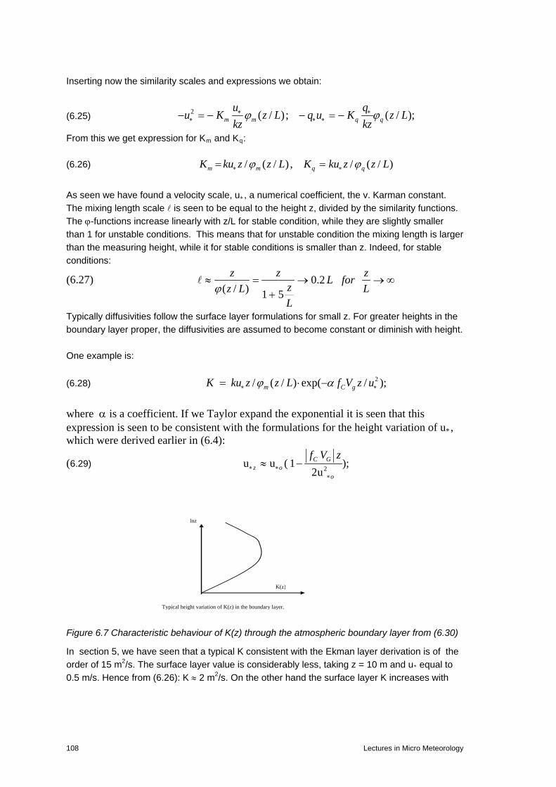
Inserting now the similarity scales and expressions we obtain:

(6.25) 2 ( / ) ; ( / );m m q qu q

u K z L q u K z Lkz kzϕ ϕ∗ ∗

∗ ∗ ∗− = − − = −

From this we get expression for Km and Kq: (6.26) / ( / ) , / ( / )m m q qK ku z z L K ku z z Lϕ ϕ∗ ∗= =

As seen we have found a velocity scale, u∗, a numerical coefficient, the v. Karman constant. The mixing length scale is seen to be equal to the height z, divided by the similarity functions. The ϕ-functions increase linearly with z/L for stable condition, while they are slightly smaller than 1 for unstable conditions. This means that for unstable condition the mixing length is larger than the measuring height, while it for stable conditions is smaller than z. Indeed, for stable conditions:

(6.27) 0.2( / ) 1 5

z z zL forzz L LL

ϕ≈ = → →∞

+

Typically diffusivities follow the surface layer formulations for small z. For greater heights in the boundary layer proper, the diffusivities are assumed to become constant or diminish with height. One example is: (6.28) 2/ ( / ) exp( / );m C gK ku z z L f V z uϕ α∗ ∗= ⋅ −

where α is a coefficient. If we Taylor expand the exponential it is seen that this expression is seen to be consistent with the formulations for the height variation of u∗, which were derived earlier in (6.4):

(6.29) 2u u ( 1 );2uC G

z oo

f V z∗ ∗

∗

≈ −

Figure 6.7 Characteristic behaviour of K(z) through the atmospheric boundary layer from (6.30)

In section 5, we have seen that a typical K consistent with the Ekman layer derivation is of the order of 15 m2/s. The surface layer value is considerably less, taking z = 10 m and u* equal to 0.5 m/s. Hence from (6.26): K ≈ 2 m2/s. On the other hand the surface layer K increases with

lnz

K(z)

Typical height variation of K(z) in the boundary layer.


height on to the top of the surface layer, being from 10-100 m above ground. Hence from this we must expect the surface layer to look quite different from its predicted behaviour in the section about the Ekman spiral in section 5.

Variances and Spectra.

The variances and the spectra are obviously related, since the variances derive from integration of the spectra.

The variances can be made non dimensional with appropriate scaling parameters, since we have introduced scaling parameters for each basic variable, wind, temperature and humidity. The properly scaled data can be plotted as functions of z/L. The variability of such functions with z/L is a test of the applicability of Monin-Obuchov similarity function for these variables. Generally, it is found to work for some of the variances, but not for all, reflecting some limitations to the surface layer concepts. As an example of a variance estimates, where surface layer scaling works well, we refer to σw, the standard deviation of the vertical velocity, and σθ, the standard deviation of temperature. Following the scaling philosophy presented out above, we would scale or normalise these two with u∗ and θ∗, and expect the scaled variables to be function of z/L

(6.30) ( ) ( )ww

z zf and fu L L

θθ

σ σθ∗ ∗

= =

It is seen that Monin-Obuchov similarity does indeed work well for many of these. It does not work well for horizontal velocity components, as we shall see in Section 8.

Similar experience has been found for the spectra. The scaling used is derived from a combination of the Taylor hypothesis, the Monin-Obuchov similarity, and the Kolmogorov laws for inertial range turbulence. We consider the inertial spectra for temperature and winds.

(6.31) 2 / 3 2 / 3

1 1 11/ 3 2 / 3

1 1 1

( ) ;

( ) ;u u

T T

k S k k

k S k kθ

α ε

α ε ε

−

−

=

=

Inserting the similarity functions for dissipations, we obtain.

(6.32)

2 / 31 112 2 / 3 2 / 3

2 / 31 112 1/ 3 2 / 3

( )( ) ;

( )( ) ;

u u

vk

T T

vk

k S kk z

u kk S k

k zk

ε

ε εθ

αϕ

αθ ϕ ϕ

−

∗

−−

∗

=

=

where we summarise the expressions for the dissipation functions, with v. Karmans constant denoted kvk here, because we here use k1 as horizontal wave numbers:


(6.33) 3 2( ) ; ( ) ;vk vkk z k zz zL Lu u

θε εθ

ε εϕ ϕ

θ∗ ∗ ∗

= =

The above shows that if we measure the spectra as function of wave number, the inertial subranges for several measuring heights would fall on the top if normalised as shown. If we measure time signals and analyse for frequency spectra then the Taylor’s hypothesis is used to write the k1z variable as a normalised frequency n:

(6.34) 1[ ] ;2k zf Hz z zn

u π λ= = =

Warning! : Before around 1980 n was called f, and f was called n. One has to check in older papers. We recall that in Section1, the Taylor hypothesis was formulated as:

(6.35) 1

ut x∆ ∆

=∆ ∆

which means that ω = u k1. We recall as well k1S(k1) = nS(n). The result of these considerations is that if we normalise the power spectra as indicated by (6.32), and plot the normalised spectra versus the normalised frequency n, the resulting plots will universal, and independent of wind speed, measuring height and stability. This scaling has only been derived for the inertial subrange by the above scaling arguments, but it is generally used also a larger range and is empirically found to work over a much larger frequency range, if one allows for additional dependency on the stability, z/L. As for the variances it is generally found that some of the spectra and some parts of the spectra can said to follow better these M. -O- similarity formulations, than other parts. Examples are shown on the following figure, Figure 6.8, which show all the main spectra and co-spectra in the surface layer, scaled with dissipation expressions for near neutral conditions, as described above. As additional stability dependency, Figure 6.9 shows the variation of the peak frequency with stability, showing a tendency for the spectra to move to larger n, or smaller scales, following (6.34).


. Figure 6.8. Normalised spectra, according to (6.31), for near neutral condition plotted versus the normalised frequency, n (Kaimal et al, 1972)

Figure 6.9 Variation of the normalised peak frequency, nm of the spectra in Figure 6.8 with stability. The absence of curves for unstable u and v-spectra is an indication of that these spectra do not follow the Monin-Obuchov similarity well for unstable conditions as we shall see in section 8.

Note that the co-spectra in Figure 6.8 are normalised by the total corresponding fluxes. Hence, the co-spectra show the contribution to the respective fluxes from the different frequency intervals. Aside from the low frequency part of the power spectra for the horizontal velocity components, u and v, in unstable surface boundary layer (see Figure 8.10), also other spectral characteristics


obtained within the atmospheric surface layer show deviations from the M.O. similarity illustrated in Figure 6.8 and 6.9. An example is shown in Figure 6.10. This figure illustrates that not all signal variability within the near surface layer can be characterised as surface layer turbulence in the sense discussed in section 2 as that not all variability within the boundary layer is created from boundary layer processes. In Figure 6.10 the low frequency fluctuations reflect the low frequency spectra discussed in section 2, notably the meso-scale spectra presented in Figure 2.23.

Figure 6.10. Stable spectra measured at 46m above terrain from Larsen et al (1990). The right hand figure shows 10 such spectra of the v-component. Here, the higher frequencies shows the spectral variation consistent with u∗ and z/L as discussed here, while the lower frequencies show no such variation, and are basically independent of the surface layer scaling and reflect the meso-cale spectra presented in Figure 2.23. The right hand figure shows the average of the three velocity components, u,v, and w for the 10 runs presented on the former figures. It is seen that only the w-spectrum is negligible for the mesoscale frequency range, and indeed only the w- component spectrum can be explained fully by the surface layer scaling, as illustrated in Figure 6.8 and 6.9. Just as we have considered variances and co-variance for variables measured at the one point, we may also consider correlation between variables at different points of space, various kinds of cross-variances and cross spectra involving data from different points in space. Especially we shall study correlation between velocities at different spatial points, which are important for wind load modelling.

(6.36) 2

( , ) ( , ) ( , )

( , ) ( , ) / ( , ) ( , )u i u i u i

u i u i u i u i i

S Co iQ

Coh S S x S x

χ ω χ ω χ ω

χ ω χ ω ω χ ω

= +

= ⋅ +

This first of the equation describes the cross spectrum of a velocity component at point xi and xi+χ i. In the second equation one has simplified by taking the absolute square of the cross


spectrum and normalised by the similar one point power spectrum established as geometric mean of the spectra in the two points considered. This is denoted the Coherence. Consider the correlation expression from (2.49).

(6.37) 1

( )1

( )

( , ) )

)

( , ) (

(

i ii

i i

i

i

i ku u

i k Uki

i ik

u ik

R U

e dk

S k k e dk d

S k

χ ωτ

χ τ

ω

χ τ ω δ ω ω+

+

=

=

−∫∫∫ ∫

∫∫∫

Where we have introduced the δ-function, defined in section 2, to account for Taylor hypothesis of frozen turbulence, as we have used throughout the spectral description above, with the mean wind, U, along the x1 -axis. The cross spectrum from (6.32) can now be computed from:

(6.38) 1( )1 1( , ) ( , ) )2 2

( i i

i

i k Uk iiu i u i iu i

k

S R e d e dk dS k χ τ ωτωτχ ω χ τ τ τπ π

+ −−= =∫ ∫∫∫

Here we use another δ-function

(6.39) ( )1

1( )2

i k Uk U e dω τδ ωτ τπ

−− = ∫

Hence we arrive to an expression for the two point cross-correlation spectrum

(6.40) 2 2 3 31

2 3

( )/ )2 3 2 3( , ) ( , , ) i k ki U

u i uk k

S e S k k e dk dkU

χ χωχ ωχ ω += ∫∫

Which shows a cyclic variation between the Co and the Q part essentially controlled by the exp(iωχ1/U) or the phase delay. From (6.36) we now obtain the coherence as follows, using horizontal homogeneity in (6.32):

(6.41) 2 2 3 3

2 3 2 3

2 2

2( ) 22 3 2 3 2 3 2 3

( , ) ( , ) / ( )

( , , ) / ( ( , , ) )

u i u i u

i k ku u

k k k k

Coh S S

S k k e dk dk S k k dk dkU U

χ χ

χ ω χ ω ωω ω+

= =

= ∫∫ ∫∫,

Based on this very simplified picture we conclude that displacement along the mean wind direction will influence the phase not the coherence that will remain equal to unity. Only displacement perpendicular to the mean wind will reduce the coherence because the numerator will be smaller than enumerator in (6.37). The model can be expanded assuming isotropy spectral relations, as given in section 2. This is done in Kristensen and Jensen (1979), with good results. However, we can already point to many limitations to the validity for this modelling, as also pointed out by Kristensen and Jensen (1979) and Kristensen et al (1981): We know that there will be a reduction of correlation also along the mean wind direction. For many scales, relevant flow fields are not isotropic, especially in the z-direction where it is not even homogeneous. Therefore, we shall cite some of the empirical expressions e.g. Davenport (1961), which are based on the simple exponential model below, with the coefficient a being specified for different displacement and ambient conditions.


(6.42) ( ) exp( / )Coh f af Uχ≈ −

Where the coefficient a is dependent on the separation and direction of the separation χ, longitudinal vertical or lateral and also depends on stability, reflecting the increased larger scale contribution to the spectrum for increased instability. However, the stability effects seem not as clear as for many of the other parameters studied in this section. Additionally, we must expect to have to include the measurement height, z, because the turbulence depends on the measurement height. The frequency is now in Hz. The following estimates of the a-factor for lateral and vertical displacement, indicated by y and z respectively, but not including stability effects, are from Panofsky and Dutton (1984), but many other formulations exist, e.g. Kristensen et al (1981)

(6.43)

10 11 50 4

10 11

60

y yy

zz

wx

a forz z

az

aU

χ χ

χ

σ

≈ + → →

≈ +

≈

The values indicate that the coherence for pure vertical and the pure lateral displacement behave rather similarly for close to neutral conditions, the limiting value is indicated for ay only though. The longitudinal coherence reflects eddy decay time relative to advection time. Additional to displacement direction, we can also consider the three different wind components of the turbulence, stability has been shortly discussed. Finally should be mentioned that the expressions in (6.38) are found from 3D surface layer turbulence. Also the low frequency parts of Figure 6.10 give rise to coherence that has now been parameterised, and behave quite differently from the boundary layer turbulence normally considered in these notes (Vincent et al, 2012) We now leave the discussion of the atmospheric surface boundary layer. The next figure shows the boundary layer, as we understand it now. We have especially studied the surface layer, and the scaling expressions that apply within this layer. When we say that they apply within the surface layer, it raises the question of what we expect to be describable within the surface layer. The short answer is local variables, meaning variables that can be defined within this layer only. We have seen the variables, representing fluctuations, can be considered local, vertical gradients and horizontal gradients likewise. Mean values cannot be considered local, in the sense that they can be determined from within the surface layer only. To determine wind speed and temperature we have to integrate the gradients from a surface value and up, forcing us to introduce z0 and z0T, both parameters, laying outside the turbulence boundary layer. With these limitations we have found the formulations to work reasonably well within the surface boundary layer of the atmosphere. Some the expressions that can be derived do not work, and often it is argued that influence from nearby layers is penetrating into the surface layer. Recall that the idea of distinct layers is really in contradiction with another idea, the ideas of the boundary layer being immersed into a soup of eddies of all sizes and orientations.


Figure 6.11. Schematic drawing of the atmospheric boundary layer with sub-layers. The surface boundary layer is seen between hsl and hs. Between the surface boundary layer and the surface we have a viscous interfacial layer, where also the molecular diffusivities are important, because the turbulence is inhibited by the nearness of the ground. Above the surface layer is the boundary layer proper, where also the turning of the wind and the structure at the exchanges with the free atmosphere are important. In the following section we shall consider the Viscous interfacial layer. Appendix 6A. Dimensional analysis. The Buckingham PI-theorem. In the main text, we have simplified the momentum equation to be valid for the statistical stationary and horizontally homogenous surface boundary layer. Defining suitable characteristic scales we could argue for the functional form of relevant dimensionless meteorological quantities. Here, we shall introduce a more formal method of dimensional analysis leading to similar expressions, the so called Buckingham Pi theorem, which we have summarized from Jensen and Busch (1982). Assume that a physical system is described by a number of physical quantities Q1, Q2, Q3, ----, Qn., through the equation: (6A.1) 1 2( , , , ) 0nF Q Q Q− − − =

Equation (6A.1) is dimensionally homogeneous, meaning that that it is independent of the dimensional units chosen. The n physical quantities Qi, are assumed to involve r independent

Ln (z)

h

h s ∼ 0.1h

Surface Boundary Layer

Boundary Layer Proper

h sl

?

surface

Viscous interfacial layer


physical units, like time, length, mass etc. Now the Pi theorem states that (6A.1) is equivalent to another function: (6A.2) 1 2( , , , ) 0.n rf π π π −− − − =

Here π1, π2, π3,---, πn-r are independent dimensionless power products of the Q quantities. Note that that letting the function equal to zero, is to be understood such that the function value remains constant for all allowable values of the parameters. Therefore, the solution of (6A.2) means finding constrains between the parameters to allow f (-) to remain constant. The Pi theorem allow one to find the minimum number of dimensionless parameters needed for a complete description of the physical problem, described by (6A.1). Normally the Pi theorem cannot provide information about the functional form of the solution to (6.A.1). It must be determined by other means, mainly through measurements. As example we apply the Pi theorem to the simplest possible version the surface layer formulation, then neutral wind relations in (6.7a), where we again assume that the wind profile must depend on the friction velocity and the height. However, we neglect the dissipation from (6.7a), because it assumes additionally that the there is local balance between production and dissipation of kinetic energy. Hence, we can write (6A.1) as:

(6A.3) ( , , ) 0.uF u zz ∗

∂=

∂

Here we have 3 Q quantities, 2 dimensions (time and length). Hence we need only one dimensionless parameter in the f-function, we obtain:

(6A.4) ( ) 0z ufu z∗

∂=

∂

This in turn in implies the validity of (6.7b), neglecting the dissipation, and leading to the logarithmic profile.

(6A.5) 1z u

u z k∗

∂=

∂

Note that just in main text of this section, the important assumption is the number of parameters that describe the physical problem. In this spirit we now continue by including the effect of buoyancy effects

(6A.6) 0

( , , , ' ', ) 0.u gF u z wz T

θ∗

∂=

∂

Now we have three basic dimensions, length, time and temperature and five Q-quantities, meaning that we need two π-quantities, e.g.:

(6A.7) 1 2 30

; ' 'z u z g zwu z u T L

π π θ∗ ∗

∂= = =

∂,

Where we have reintroduced the Monin-Obuchov stability length L., from the main text of this section. Hence the f-function looks as follows


(6A.8) ( , ) 0,z u zfu z L∗

∂=

∂

This implies that:

(6A.9) ( )mkz u zu z L

ϕ∗

∂=

∂ ;

Where the v.karman constant, k has been introduced from (6A.5) and also introduced the stability function for the wind profile, we found in the main text of the section. The dimensional analysis has been found very useful in meteorology, using dimensional argument for relations between quantities. However, it does not always work properly, often because one neglects parameters in the analysis that should have been involved.


7. Near surface viscous layers, roughness lengths: z0 and z0T, interfacial exchange.

Behaviour of profiles and flow close to the ground. The behaviour of the velocity profile very close to the ground is illustrated below.

Figure 7.1. The logarithmic and the actual wind profile near the ground. δ is the lower height where the logarithmic profile applies, z0 is the roughness length. The x- points show actual profile values. The profile on the figure is a standard:

(7.1) 0

( ) ln( );u zu zk z∗=

δ is the lower height of validity for the logarithmic profile. Note that z0 is below δ, so z0 is the extrapolated height where the logarithmic wind profile attains the true value of the wind at the ground, namely zero. As a rule of thumb, δ ≈ 10z0. Below δ the wind is influenced by the individual roughness elements as well molecular viscosity. If the surface is flat viscosity dominates we can estimate δ from the flux divergence terms in the average momentum equation, e.g. from (3.83), where the two last terms read:

(7.2) 2

2 ( ) ,i ji

jj

u uu u u wx z zx

ν ν′ ′∂∂ ∂ ∂ ′ ′− = −

∂ ∂ ∂∂

where we, as usual, have assumed gradients only in the z-direction. We have earlier argued that the molecular term could be discarded due to the much larger turbulence term. However, close to the ground the profile gradient becomes large enough for the molecular term to dominate. Inserting the surface layer expressions and inserting δ as the height where the molecular an turbulence terms are equal, the equation above reads:

(7.3) 2( ) ( )uu u w u

z z z k kuνν ν δ

δ∗

∗∗

∂ ∂ ∂′ ′− = + ⇒ ≈∂ ∂ ∂

Since ν∼0.15 cm2s-1, and u∗ is typically > 10 cm/s, δ is seen to be around 0.1 mm, so the above considerations are valid only when roughness elements are below that height.


To see what happens in the more general situation, we take the non-averaged momentum equation for the u-component, e.g. (3.72), using incompressibility to rewrite the advection term.

(7.4) 2

2

1 0.j

j j

uuu p ut x x x

νρ

∂∂ ∂ ∂+ + − =

∂ ∂ ∂ ∂

Introducing explicitly the components, u, v and w, and rearranging slightly, we obtain:

(7.5) 2 1( ) ( ) ( ) 0u u u uu p uv uwt x x y y z z

ν ν νρ

∂ ∂ ∂ ∂ ∂ ∂ ∂+ + − + − + − =

∂ ∂ ∂ ∂ ∂ ∂ ∂

Notice, we still do not average. We now integrate the equation from the true surface z = η(x, y, t). The time, t, is included because many surfaces move in time, with water surface wave fields as the most important example. The integration will be carried out from z = η to z = h, where h is well into the turbulent surface layer with M.O. similarity, logarithmic profiles etc., see figure 7.2.

x Figure 7.2. The actual surface, η(x, (y), t), the scale height δ, and a height within the turbulent surface layer, h. The integration looks as follows:

(7.6) 2 1( ) ( ) ( ) 0h h h

hu u u udz u p dz uv dz uwt x x y y z η

η η η

ν ν νρ

∂ ∂ ∂ ∂ ∂ ∂+ + − + − + − =

∂ ∂ ∂ ∂ ∂ ∂∫ ∫ ∫

We use Leibniz’ rule to move the differentiation outside the integration to facilitate interpretation:

( ) ( ) ( ) ,h h hhdz dz h dz

x x x x x xη η η

φ η φ ηφ φ η φ φ η∂ ∂ ∂ ∂ ∂ ∂= − + = −

∂ ∂ ∂ ∂ ∂ ∂∫ ∫ ∫

Where we have used that h is a constant height. Hence (7.6) takes the form:


(7.7)

[ ] [ ]

2

2 2

1( ) ( ) ( )

1 1( ) ( )

( ) ( ) ( ) ( ) 0

h h hh

h h

h

h

u u u udz u p dz uv dz uwt x x y y z

u uudz u u p dz u pt t x x x x

u u u uuv dz uv uw uwy y y y z z

ηη η η

η ηη η

η ηη

ν ν νρ

η ην νρ ρ

ην ν ν ν

∂ ∂ ∂ ∂ ∂ ∂+ + − + − + − =

∂ ∂ ∂ ∂ ∂ ∂

∂ ∂ ∂ ∂ ∂ ∂ = + + + − + + − + ∂ ∂ ∂ ∂ ∂ ∂

∂ ∂ ∂ ∂ ∂ ∂+ − + − + − − − =∂ ∂ ∂ ∂ ∂ ∂

∫ ∫ ∫

∫ ∫

∫

The terms in square brackets are for later use. Next we consider the no-slip conditions between the air and the surface, η(x,y,t), meaning that an air particle at the surface remains there. The speed of a surface particle can be written:

(7.8) 0;dw u vdt t x yη η ηη η η η∂ ∂ ∂

= = + + =∂ ∂ ∂

Multiplying this equation with u, it is seen we can eliminate the terms within the square bracket in the integrated momentum equation. The equation now takes the form:

(7.9)

2 1 1( ) ( )

( ) ) ( ) ) 0

h h

h

h

u uudz u p dz pt x x x x

u u u uuv dz uwy y y y z z

ηη η

η ηη

ην νρ ρ

ην ν ν ν

∂ ∂ ∂ ∂ ∂+ + − + − +

∂ ∂ ∂ ∂ ∂

∂ ∂ ∂ ∂ ∂ ∂+ − − + − + =∂ ∂ ∂ ∂ ∂ ∂

∫ ∫

∫

We now takes the mean value and assume, as usual, stationarity and horizontal homogeneity for mean quantities, in the turbulent surface layer, where all integrals get the most of their contributions, collecting all terms without integration first:

(7.10)

2

( ) ( ) ( )

1( ) ( ) 0

h

h

h h

p u u u uudz uwt x z x x y y z

u uuv dz u p dzy y x x

ηη

η η

η η ην νρ

ν νρ

∂ ∂ ∂ ∂ ∂ ∂ ∂ ∂+ + − − + −

∂ ∂ ∂ ∂ ∂ ∂ ∂ ∂

∂ ∂ ∂ ∂+ − + + − =∂ ∂ ∂ ∂

∫

∫ ∫

or:

(7.11) 2) ( ) ( ) ;h hp u u uwu u

x z x x y yηη η ην

ρ∗∂ ∂ ∂ ∂ ∂ ∂

− = = + − −∂ ∂ ∂ ∂ ∂ ∂


The two last integrals above will be close to zero in the turbulent surface layer, where they get most of their contributions. The first is for the lateral velocity, when the coordinate system is aligned with the mean wind in the u-direction. The second term is simply the balance between advection and pressure forces in the mean wind direction. As usual, when we are in the turbulent surface layer we can neglect molecular terms. The result can then be formulated as, that the turbulent momentum flux in the turbulent surface layer, in the near surface layer is taken over by a mixture of pressure forces on terrain features, called form drag and included in the first term, and molecular transport. For the molecular terms the first are usually considered the most important. The two last are normally neglected except in wave growth theories where they are considered important. Next we study how the scalar variables are transported towards the surface through the viscous interfacial layer. We have a similar profile expression in the turbulent surface layer:

(7.12) 00

ln( );T

zk zθ

θ θ ∗− =

We have a similar figure for temperature as figure 7.1 for wind speed:

Figure7.3. The temperature profile close to the ground. ∆ is the lower height of validity for the logarithmic profile, shown as a straight line.z0T is the “roughness length for temperature. Corresponding to the momentum equation starting from (3.58) and neglecting the humidity term:

(7.13) 2

2 0j

j j

ut x xθ

θθ θν∂∂ ∂

+ − =∂ ∂ ∂

The equation is similar to the momentum equation for the u component, which we used to study the surface stress. The only and important difference is the absence of the pressure term. Hence we can find the result directly, without redoing the derivation, we just did. (We also here use η(x,y,t) as the actual surface).

(7.14) ) ( )hwz x x y yθ ηθ θ η θ ηθ ν ∂ ∂ ∂ ∂ ∂

− = − −∂ ∂ ∂ ∂ ∂


This means that close to the surface heat and all other passive scalars must be transported by the molecular transport only, as opposed to surface stress that could use pressure as well in the form of form drag. Hence, for many surfaces scalar transport is fundamentally different from the momentum transport close to the surface. Roughness Formulations and Parameters The purist attitude is that the z0 parameters are simply integration parameters, when Monin-Obuchov profiles are integrated. It is a height where the variable attains its surface value (zero for wind speed). From another point of view it is a characteristic of the surface, being responsible for the atmospheres friction and general coupling and exchange with the surface. Determination of z0 is then a field were knowledge about the roughness of specific surfaces has been determined mostly experimentally but also with some theory. Below we cite such formulas for specific surfaces. Surfaces with characteristic surface elements The roughness is derived from the density and shape of the roughness elements: (7.15) 0 0.5 / ,z h S A A S≈ ⋅ ⋅ >>

Here h is the height of the individual roughness elements. S is the crosswind area of a roughness element, and A is the average surface area for each roughness element (Lettau, 1969). Dense vegetation, canopies, cereal fields etc. One of the simplest formulas here is:

(7.16) 01 2( ); ;3 3

z h d d h= − ≈

Where h again is the height of the canopy, d is the so-called displacement height. The displacement height is generally introduced over denser vegetation, as illustrated below. Here some of the canopy height contributes to a change in surface level, rather than to roughness. Figure 7.4 Illustration of roughness elements having both a roughness length and a displacement height, here for a forest canopy (Stull, 1991)


Theoretical one can estimate the displacement height as the level where the frictional forces attacks the surface. Experimentally one has to fit two parameters from a logarithmic expression instead of just one, z0.

(7.17) 0

)( ) ln( );u z du zk z∗ −

=

The equation shows consensus about how to introduce d into the logarithmic profile equation. As seen from the forest picture, Fig 7.4, above the exact profile becomes quite different from the turbulent surface layer profile. This is illustrated also on the next figure showing the profile from just above and down through a cereal canopy. Figure 7.5. Wind profiles above and through a cereal canopy, not being logarithmic, but rather by an exponential variation around the crop height.

Roughness of water surfaces. Over the ocean the roughness elements are associated with the wind driven surface waves. Observing that the waves were generated by the wind force on the surface, proportional to u∗

2, and restrained by gravity, Charnock(1984) proposed a simple relation for z0:

(7.18) 2

0uz

u gνβ α ∗

∗

= +

The first term is later introduced for low wind situations, with few waves and wave roughness elements, where molecular viscocity becomes responsible for the momentum transport close to the surface, see equation (7.3). The coefficient, β, is usually taken as about 0.1. The coefficient α is found to be very small and quite variable between 10-2 and 3·10-2, dependent on site and situation. Many more complicated expressions, but the scatter of the data, around both (7.18) and the more complex expressions, makes experimental evaluation difficult, see appendix 7A . The fact that the numerical coefficient is so small is normally taken as indication of that all parameters have not been include. (Hansen and Larsen,1997). The water roughness is usually quite small, mostly less than a few tens of a millimetre. Indeed water is one of the least rough surfaces in nature. As seen it also changes with wind speed, a


thing that actually happens for many other surfaces, like a blowing sand surface, a vegetated surfaces, where the air does not just exchange momentum but also energy with the surface, by moving part of the surface around, waves for the water, sand particles for sandy surfaces and leaves and branches for vegetation. See also Appendix 7A. Seasonal and other changes of roughness. Many surfaces show changes of roughness with season because the roughness of vegetated surfaces change with the seasonal changes of the vegetation or due to aspects like snow and ice cover in the winter. Below we show a figure of the seasonal change of the roughness for typical Danish fields.

Figure7.6. Seasonal variation of the roughness length, z0, measured for three agricultural fields, 2, 3 and 4 in Western Denmark (Sempreviva et al, 1989)

-

Figure 7.7. The figure shows the seasonal roughness variation as measured from several small masts and one tall mast in the same area. Also the modeled area roughness is reported. The seasonal variation of all data and models is clearly seen.(Hasager et al., 2003)

The measured roughness in figure 7.6 and 7.7 are obtained from small masts each placed in a field with a characteristic crop. The measured landscape roughness in Figure 7.7 is obtained from a tall mast. The importance of hedges for the landscape roughness is emphasized. Additionally, many types of vegetation show z0 to be a function of wind speed, a little like water because vegetation is moved by the wind, and therefore energy is supplied to the vegetated surface just as for the wavy surface of water or wind farm, see below. Also stability influences

0

0.05

0.1

0.15

0.2

0.25

0.3

1 2 3 4 5 6 7 8 9 10 11 12

Month

Ro

ug

hn

ess

(m)

Landscape 1998Landscape 1999Spring barley ISpring barley IIWinter barleyWheatGrassMaizeBeetsModel with hedges


z0, being smaller for stable conditions, due to inhibited interaction between the atmosphere and the surface for strong stability, see Zillitinkevich et al. ( 2009). Roughness of a large wind farms

Fig. 7.8. Derivation of roughness of a very large wind farm (Frandsen, 1992). As the Figure 7.8 indicates, Frandsen (1992) finds an expression by matching an outer logarithmic profile that reflects the roughness of the wind farm at the wind turbine hub height, h, to an inner profile that reflects the background roughness:

(7.19) 0

0

( ) 1 ln( )

( ) 1 ln( )

wf wf

U z z z hu z

U z z z hu z

κ

κ

∗

∗

= ≥

= <,

Where subscript “wf” denotes ”wind farm”. The relation between the two friction velocities are derived from the areal thrust of the wind farm as: (7.20) 2 2 2( )wf tu u c U hρ ρ ρ∗ ∗= + ,

The thrust coefficient for the wind farm (per unit area) is found by dividing the thrust of the individual wind turbines, T, with the surface area for each turbine.

(7.21)

2 2 21 2 1 2

1 21 2

1 2

1/ ( ) / ( )2 4

; ,8

T t

Tt

t T x x C U h D x x c U h

C x xc s ss s D D

πρ π ρ

π

= = ≡

→ = = =.

Here CT is the thrust coefficient for the individual wind turbines, and D the diameter of the area, swept by the blades, when the turbine works. CT is zero for non-working turbines, it then growths fast with wind speed to about one, and gradually decrease as 7(m/s) /U(h) to about 0.2 for 15 m/s, for characteristic wind turbines (Frandsen, 2007). Here, we neglect the contributions from the stationary structure of the wind turbine.

Matching the wind speeds of (7.19) in the hub height, and solving (7.20) and (7.21) for z0wf one obtains:

(7.22) 0 20

exp( ) exp( )( / (ln( / )

wftt

z h hcc h z

κ κκ

= ⋅ − ≈ ⋅ −+

,

where the approximation holds, if the background roughness is small compared to z0wf . Characteristic values can therefore be found from (7.22). Assuming h=100m and s= 7, we find that, for increasing wind speed z0wf starts being equal to z0, to increase fast with wind speed to about 1.1 m for U (h) =7 m/s, thereafter to decrease to about 0.2 m for U(h)= 15 m/s. Notice, we are talking about a fully working wind farm. If the turbines do not work, the roughness predicted by (7.22) goes back to the background roughness. At present experimental evidence is obviously difficult both because the height of the turbine structures actually exceeds the surface boundary layer, and also because the very large wind farm is not yet constructed. Consensus tables and figures summarising the roughness of landscapes. The experimental and theoretical knowledge accumulated is often collected into figures and tables. We show some below, where some are derived from the assessment of roughness from terrain inspection, which is an essential part of evaluating the wind power resource for a given location. One should recall the purist view, that the roughness length is a constant of integration for a logarithmic wind profile. However, as discussed above, it can also be related to the physics of the processes in the interfacial layer. However, roughness length scales for larger features, like buildings, forests and wind farms that are obviously penetrating through the whole turbulent surface layer, where the logarithmic profile is supposed to exist, as well as for whole terrain types still raises interpretation questions. Indeed, for such terrain forms, the roughness seem to be stability dependent, reflecting that the roughness elements now reach into the turbulent surface boundary a layer (Zilitinkevich et al,2006) . In spite of these complications, the roughness length is obviously a relevant feature also here, at least in a qualitative sense, since the terrains in question can be said to exert a friction with the atmosphere. Here, it is mostly be used in connection with numerical models that need an expression for the surface drag, also for these types of terrain. Aside from the inclusion of very large terrain features, relative to an interfacial layer, you will notice that many roughness aspects of a terrain are only partially, if at all, included, as indeed the roughness length is a measure of the friction between the atmosphere and the ground. However, it is also a practical parameter, which must be deductible without too much monitoring and complication Here we list a few of the complications: Figures 7.7 and 7.8 illustrate the dependency of roughness length on type of surface vegetation, and its changes. Some of these changes are natural, but for agricultural fields, farmer´s decisions on growing and harvesting periods are also important. We have seen that the roughness of water and wind farms depends strongly on the wind (for the wind farm, if it operates), so it does for sand (if it is dry) and to some extent for all vegetation that can be moved by the wind.


All landscapes can become snow covered and all low and flat landscapes covered with water. These aspects have a strong season and location dependency, but will also depend on random factors like the weather.

Figure 7.9 Terrain with roughness corresponding to roughness class 0, water areas with z0 ≅ 2⋅10-4 m. The class comprises seas, fjords and lakes. (Troen and Petersen, 1980)

Figure 7.10 Terrain with roughness corresponding to roughness class1, open areas with a few wind breaks, z0 ≅ 0.03 m The terrain appears to be very open and flat or gently undulating. Single farms and stands of trees and bushes (Troen and Petersen, 1980) .


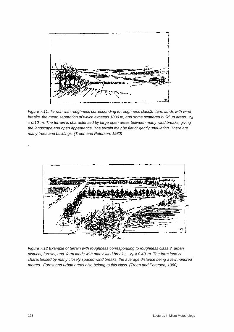
Figure 7.11. Terrain with roughness corresponding to roughness class2, farm lands with wind breaks, the mean separation of which exceeds 1000 m, and some scattered build up areas, z0 ≅ 0.10 m. The terrain is characterised by large open areas between many wind breaks, giving the landscape and open appearance. The terrain may be flat or gently undulating. There are many trees and buildings. (Troen and Petersen, 1980) .

Figure 7.12 Example of terrain with roughness corresponding to roughness class 3, urban districts, forests, and farm lands with many wind breaks,, z0 ≅ 0.40 m. The farm land is characterised by many closely spaced wind breaks, the average distance being a few hundred metres. Forest and urban areas also belong to this class. (Troen and Petersen, 1980)


Figure 7.13. Schematics of terrain types, roughness classes, and z0 – values. (Troen and Petersen, 1980).


Figure 7.14. Schematics of terrain types, and z0 – values. Note some roughness variation for similar terrain is indicated.( Stull,1991).


Scalar Roughness, z0T, z0q etc. There are two differences between the study of scalars and velocity in the viscous interfacial layer. It is simpler because we know that fluxes have to be carried as molecular transport. It is more complicated experimentally, because the scalar roughness is the height, where the profile attains the surface value of the scalar, meaning the way one determines the surface value now becomes important for the value of the roughness. For velocity it is simpler because we know that the surface value of the velocity is zero or close to zero. We shall now reconsider the figure 7.1, we used above, this time for the temperature profile.

Figure7.15. Temperature profile close to the ground. ∆ is the lower height of validity for the logarithmic profile, shown as a straight line in the logarithmic plot. The x-points show actual profile values. We consider the height ∆ to be both in the turbulent layer and in the diffusive layer. We can then establish an equation for the flux-gradient relationship in both layers.

(7.23) 0

0 0

0

ln( ) ln( );

( ) / ;T T

Hk z ku z

H θ

θθ θ

ν θ θ

∗∆

∗

∆

∆ ∆− = = −

− = − ∆

Equating the temperature gradients in the two equations we get:

(7.24) 0

0 0 0

ln( ) ln( ) ln( ) ,T T

z kuz z z θν

∗∆ ∆= + = ∆

where we, somewhat artificially, have introduced z0. We can now formulate an expression for z0T/z0.

(7.25) 0

0 0

ln( ) ln( ) TT

z kukX

z zθν∗ ∆

= ∆− ≡

(7.26) 0

0 0

, ln( )TkXTT

z kue with kX

z zθν− ∗ ∆

= = ∆−

We have no simple way of solving for ∆. Instead we try different and reasonable formulations for ∆, and see that they result in the same kind of differences between z0 and z0T. 1) ∆ ≈ν/u∗. This is the smooth surface transition we derived in the beginning of this section. It is the height where the strength of turbulence flux equals that of the molecular diffusivity. For this assumption we find the following expression for XT:


(7.27) 0

0

00

1 1ln( ) Pr ln( Re ) ;

Pr ; Re ;

TXk u z k

u zwith

θ

θ

ν νν

νν ν

∗

∗

= − ≡ +

≡ =

where we have used the definition of Pr = Prandl Number, and Re0 = the roughness Reynolds Number. The Prandtl Number is a special case of the Smidt Number for a general scalar, Sc = ν/νd, where νd is the Brownian diffusivity of this particular scalar in air. Inserting the expression for XT, the expression for the ratio between z0T and z0 becomes.

(7.28) Pr 100

0

ReTkX kTze e

z− − −= = ⋅

We now consider another assumption for ∆. 2) ∆ ≈ αz0, that is ∆ is proportional to z0. Inserting into the expression for XT, we get:

(7.29) 00ln( ) Pr Re ln( ).T

u zkX k k

θ

να α α αν ν

∗= − = −

(7.30) 0Pr Re0

0

T kkXTze e

zαα −−= =

Although the resulting equations are different, they both yield that z0T /z0 diminishes with growing Pr Number and with growing Roughness Reynolds Number. To see the actual differences, we will have to go to data, such as is shown on the next figure, which shows result from Brutsaert (1982) on XT. Typically, we have conditions with Reynolds Number between 0.5 and 200. The lowest curve on the figure corresponds to Pr = 1.20, while Pr for the lower atmosphere is about 0.7. Hence, we have to go a bit below the lowest curve. If we choose XT ≈ 5, then we find that the ratio:

(7.31) 20

0

;TkXTz e ez

− −= =

which is known as the e-2-law. These considerations apply not well for surfaces made from fibrous materials, because for such surfaces the z0T and z0 will also depend on different surface properties, an aspect that is not included in the analysis above, but also here their ratio is found often to be about e-2. This law seems also to apply approximately for many of the other scalar roughness. For other scalars than temperature, we change Pr to Sc, the Smidt number, and for some the Brownian diffusivity is very different from the viscocity, giving rise to Sc being very different from the above value around one. Consider molecules and aerosols as spheres, the Brownian diffusivity can be derived from Einsteins formula (Chapman and Cowling, 1970):

(7.32) 3d

kTd

νπνρ

=

Here, k is the Bolzmann constant, and we have used subscript d to indicate any particle, with diameter d, molecular or larger. For a typical molecule in air, we have d= 10-10 m, with ν ∼νd. Aerosols typically with d= 10-9-10-5m with νp 10-2- 10-8 cm2/s and Sc ranging from 10-107. For such small diffusivities particles have obvious difficulties ever reaching the surface, which is consistent with that z0d being close to zero in (7.28 and 7.30). Indeed one has found the


modelled surface flux to be too small, which has led to modifications of the models of the near surface layer to involve other processes than Brownian transport, to allow sufficient particle flux through the layer to describe experimentally found particle flux to the surface. Additionally also the aerosol dynamics is expanded to include impaction, gravity and slip between the air and the aerosols (Liss and Slinn, 1983, Fairall and Larsen, 1984). However, here we shall not go further into this subject.

Figure 7.16. The figure shows experimental data on ln(z0/z0T)/k = XT in (7.22) versus the roughness Reynolds number Re0 = u*z0/ν for different Prandtl and Smidt numbers. Note that the reasoning above, applied to heat flux, apply to all scalars, for which reason the Schmidt numbers are cited as well. The figure is taken from Brutsaert (1982). The solid curves correspond to XT= 7.3Re0

1/4 Sc1/2. The Smidt number is the ratio between the viscocity,ν, and the relevant diffusivity; ν/νd for the Smidt number and ν/νθ for the Prandtl number.

Figure 7.17. Schematics of the different sub-layers within the atmospheric boundary layer. We are now about leave the considerations about the viscous atmospheric interfacial layer. As seen in the last figure, we have been able to update the figure Micro Scale 6 about the different layers with new information. In the next section we shall revisit the total boundary layer,

XT


especially the part that is above the turbulence surface layer. This is the part, for which, we derived the Ekman spiral in section 5. Deeper into the interfacial layers. Before leaving the interfacial layers, we shall take a short discussion of their general characteristics. They are the layers, where the atmosphere handshakes to the non-atmospheric layer below, through at least one boundary condition. In the discussions above, we have used the surface values of wind speed, temperature and humidity as examples. We have seen that only for wind speed over solid land were the boundary condition so simple, u0 = 0 that there was an effective decoupling between the atmosphere and the soil below with respect to speed. For all other atmospheric variables, there is no such decoupling, because their near surface value in the air will have relation to their near surface value in the medium constituting the surface. In general the surface condition either must be measured or determined by modelling systems determining the variables below or at the surface. These systems will then as upper boundary conditions have the lower boundary values for the atmospheric system. Hence, the two systems have become coupled, as they are in the physical world, of-course. Examples: For wind speed over water or other moving surfaces, the wind speed is not zero at the bottom, and the surface stress influences the conditions within and on the surface, which will again influence the surface stress. For forecasting of conditions above and in the ocean the exchange across the interface is so important for the outcome of the forecast that coupled models now dominates the fields, see also appendix A . The temperature of a surface is typically forced by the radiation balance at the surface, incoming solar radiation and outgoing longer wave radiations, and the heat fluxes (sensible plus latent) to the atmosphere and down in the ground, see section 11. The humidity at the surface will be a complicated function of the water budget within the soil and the water flux above the soil. Only over free water surfaces humidity becomes simple, because the water vapour pressure at the water surface will be the saturated water vapour pressure at the temperature of the water surface. Just as the heat balance at the surface will be influenced by evaporation and water vapour fluxes, also the water vapour budget will be strongly influenced by the heat budget. From a modelling point of view, both surface values and surface fluxes of many variables are neither very relevant nor well defined. They are not well defined because many surfaces are not well defined on closer inspection, like e.g. vegetated surfaces. They are not relevant, because the relevant flux at the surface takes place between a reservoir in the air and a reservoir below the surface. Examples here are trace gas exchange across the water interface, which is parameterised on the difference between the water concentration and the air concentration, both specified well away from the interface. Also gas fluxes between vegetation and the atmosphere will often be controlled by the concentration difference within the vegetation and in the atmosphere, coupled through a stomata resistance. For both cases the exact values at the


surface become irrelevant, because the atmosphere and the layer below is coupled now through the boundary flux only. Resistance modelling A useful concept for such considerations is the resistance-models that allow us to handle such surface flux considerations. In the next figure, we have an upper and a lower layer, where the concentration of a substance is controlled by a differential equation

(7.33) ( , ) , ( , )DC DCF C and G CDt Dt

= ⋅ = ⋅

The solution of these equations involve among others the boundary values and fluxes

Figure 7.18. Illustration of exchange between to volumes, one above and one below the surface, The fluxes between the two layers are determined under the assumption of stationarity and horizontal homogeneity, meaning that the vertical flux is constant through the layers. Hence we have: (7.34) s vi bsF F F F F+−≡ = = = ,

where F+- is the flux across the interface. For Fs we find, for example using K-theory, which we developed for surface layer turbulence:

(7.35) 1( ) ( );

( / ) ( / ) s s

ms h h

C C s a

zku z kuC CF K C C C Cz z L z z L h rδ δϕ ϕ δ

∗ ∗∂ ∂= − = − ≈ − ≡ −

∂ ∂ −

where we have defined a resistance for fluxes through the turbulence surface layer, ra, subscript a stands for aerodynamic. Similarly we get for the flux through the viscous interfacial layer:

(7.36) 0 01( ) ( )vi

C DF D C C C Cz rδ δ

δδ + +∂

= − = − − ≡ −∂

As of now we have presented no model about the fluxes at the interface and below the surface, they may be trough stomata or roots or involving chemical bindings or similar strange pathways.


Whatever they are, we assume that the processes carrying the fluxes allow us to cast them in the resistance frame, hence:

(7.37) 0 0 01 1( ) , ( ).bs d

bs

F C C F C Cr r+− + − −+−

= − = −

The solution of this system is easily seen to be: (7.38) ( ) ( );

sa bs h drF r r r r F C Cδ +−= + + + = −

This system shows analogy with Ohm’ s law, with the flux as a current and the concentration differences as voltages. The total resistance of a flux path is seen to equal the sum of resistances, similarly a parallel pathway for the fluxes, can be computed with a parallel resistance that will combine with the total like parallel resistances in electric network. Finally, the fact that all the fluxes are equal means that the concentration gradients will be large, where the resistance is large, and vice versa. A limitation to the resistance concept is need for stationarity for the system to work that is for the flux to be constant through all layers. Hence, when the transport time along a flux path way become too long, one must change to differential equations in the different layers and the modelling becomes more complex. The last figure shows the system of layers usually employed when estimating fluxes across the

air –sea-surface, using a resistance formulation: Figure 7.19. Schematics of a full resistance model for the atmosphere –ocean exchange. All the fluxes shown on the figure are to be modelled by the dominant processes at each layer..


Discussion. In this section we have discussed the characteristic of the surface boundary conditions for the atmospheric boundary layers. We have seen that they typically are specified in terms of roughness parameters and surface values. Velocity has the simplest surface value and roughness characteristics, in that the wind speed is zero at the ground due to the no-slip condition. We have seen that in general the surface characteristics involve the momentum transport to the surface by Brownian diffusion and through flow separation around roughness elements. Hence, there is a minimum roughness, as given by the molecular term in (7.19). Aside from this, at the simplest the roughness can be described as a landscape parameter, as is presented by some of the characteristic landscape drawings and the schematic summary of landscape and roughness. In the next approximation, the roughness may be expected to depend on wind speed, strongest for water surfaces, but also for dry sand and vegetation. Characteristic seasonal changes must be expected as well, reflecting seasonal differences in the vegetation (leaves and growth of agricultural crops) and ice and snow cover (of obvious importance, but not discussed in the section). Indeed, the roughness changes will often be seasonal, but obviously in a detailed analysis they are associated with physical changes of the surface characteristics that in average (but not always and not only) follows the changing season. Indeed, as we pointed out, when roughness elements reach into the turbulent boundary layer, the roughness may even depend on stability, because the eddies encountered are now modified by stability. Close to the surface the transport of scalars can utilise only the molecular diffusion, as opposed to momentum transport. We have accounted for this through a roughness Reynolds number dependency. The scalar roughness is shown to be velocity dependent as well, both through the wind roughness and in their relation to this roughness, involving the roughness Reynolds number. They furthermore has an uncertainty related to that the surface value of the scalars is not forced to zero by the no-slip condition, as for velocity, but must be determined independently from measurements or modelling. Additionally, it should be pointed out that it often is not possible to write a functional dependency between z0 and the scalar roughness, because they can dependent on different features of the surface and involve additional processes in the flow. In spite of these uncertainties the scalar roughness for many substances is often found, following a roughness Reynolds number relation, giving about a tenth of the wind roughness, when this roughness involves the flow separation around roughness elements. If modelling of the surface fluxes and values are chosen, one must consider also the conditions in- and below the surface as presented in this section through the resistance modelling, and in section 11 about the energy balance at the surface.


Appendix 7A. Characterization of a water surface. The marine ABL has quite distinct features compared to the land ABL, reflecting the special characteristics of the water both dynamically and thermally. Therefore, we shall shortly summarize these characteristics in this appendix. The water is semi transparent meaning that the radiational heating and cooling is distributed downwards. Additionally the water is very efficient in redistributing heat vertically. The surface waves and circulation systems, like the Langmuir Cells, combined with turbulence give rise to extensive mixing. Additionally, when heated from above, the surface water evaporates, and it will start sinking; now being heavier, because it retains the salt from the evaporated water. If the surface water cools, it also becomes heavier due to the cooling and sinks. All this give rise to an intense mixing in typically the upper 10 meter of the ocean. In the heat exchange with the atmosphere the water therefore constitute a very large heat reservoir that only can change its temperature slowly, and additionally has its own heating and cooling from the ocean currents. Indeed when an air mass moves over an ocean for enough time, it ends up at the temperature of the ocean surface. For these reasons the homogeneous marine ABL is always close to neutral. The diurnal radiation cycle shows very little influence on the water surface temperature, although it can be measured, but typical amplitudes are less than a few tenths of a degree (Pena et al, 2008). The annual radiation cycle on the other hand has significant influence on the sea temperature, because they involve enough heat and time to change both the temperature and the depth of the mixed layer. However, stable and unstable conditions happens over the ocean as well on shorter timescale, , but they are mostly transitional, associated with air masses moving across water surface with a different temperature, either coming from a nearby land or associated with moving weather systems. We shall return to these phenomena when coming to the inhomogenous and instationary ABLs in section 9. The sea is also an obvious source of water vapor, indeed over the ocean, q0, the surface value of the water vapour mixing ration, is derived from the saturated pressure at the surface temperature. The ocean is also a source of liquid water in the form of sea spray converting to marine aerosols. In winter time the spray is the source of icing on ships and offshore structures. The roughness elements over water mostly take the form of small steep waves of a wave length of around 5 cm, although momentum can be transferred also by larger scale breaking waves. The ocean surface is depicted in Figure A1. Since the roughness is associated with the waves and the waves are generated by the wind and modified by gravity, Charnock (1955) proposed that the roughness should depend on u∗ and g. A slightly updated version of the roughness for water looks as follow:

2

0 0.11 ( / , )u

z c uu gν

α ∗∗

∗

= + − (7A.1)

Which we have taken from (7.19), now with an estimate of the coefficient β , and the Charnock coefficient,α, now being a function of the phase speed of the dominant wave c, and the friction velocity, u∗, since the roughness elements will be mowing with the phase speed of the dominant waves in the direction of the wind. The term, c/ u∗, is denoted the wave age, because c increases with the duration of the acting wind∗. The Charnock coefficient,α, is varying between 0.01 and 0.07, being smallest for mid-ocean mature waves with large phase speed. A “typical” value for regional seas is 0.015, α can be a function of other parameters as well: e.g. bottom topography, swells, both modifying the waves and their direction of propagation, and very high


wind (e.g. hurricanes) results in foam covered waters that reduces β further (Makin, 1997). As seen in α (A1) may also depend on other variable, here denoted by “-“. Other variables may be a suitable expression for the wave height or wave steepness , either overall or in certain frequency bands, a characteristic wave length for the waves, etc. We shall return to this later.

Figure 7A.1. The wind

profile close to the water surface, with the wave induced vorticity and the small scale roughness element riding on the larger scale waves, with a phase speed c. Also the rotor movement of a water wave is shown.

A short summary of the surface waves is now useful; The surface wave amplitudes η( x, t) is a semi periodic statistical function of space and time. Similar to turbulence, one can consider wave spectra of either wave numbers or frequencies, connected through the dispersion relation.

(7A.2)

The wave amplitude depends on the time or the fetch that has been available for the wind action on the water surface. Young waves have small wave lengths, large steepness, and small phase speeds. The waves are generally produced with propagation along the wind direction ± 5°. Older waves are characterized by larger wave length and lower frequencies, with larger phase speeds, larger amplitudes and lower steepness. Some waves propagate from afar, generated by other wind fields. They are typically of even longer wavelength and lower frequencies .They are denoted swells. Waves can be diffracted by bottom topography. Figure A2 illustrates typical wave amplitude spectra as function of frequency. The red one pertains to coastal areas, while the black broken curve reflects more mid-ocean conditions.

2 2

2

( , ) cos( ):

(1 / ) tanh( ):

" " 1 / 1

x t a k x tdispersion relation

gk k g kdphase speed

k k kg gck k k k k

The requires kd and k g

η ω

ω γ

ωω

γ

≈ ⋅ −

= +

= ≈ =

≈ >> <<

As difference frequency regions of the spectra can propagate in different directions and with different phase velocity, one often uses the characteristics at the peak, e.g. ω

p , c

p and S(ω

p)

to characterize the whole spectrum, since the spectrum is fairly narrow with a sharp peak.

Figure 7A.2. Two characteristic spectral functions, The Pierson –Moscwitch (PM) and the JONSWAP form. The PM form is generally used over the open sea, while the JONSWAP form is used in coastal areas. (IEC6140-3, 2009) The peak frequency is found to vary with fetch as (Frank et al, 2000). Alternative to fetch one can use time since start of production with t=x/U10 .

1/3

10

2/3 5p

xgc uU

π∗

= ⋅

(7A.3)

Based on the above coefficient we can now show the Charnock coefficient,α, versus the wave age in Figure A3. It should be emphasized though that many wave fields are so irregular that the scatter around functionality depicted in the figure can be fairly large. As seen even with the selected data in the figure the scatter is large. Much of the scatter is related to occurrence of swell that per definition are not local and hence could not be expected to be scaled with local variables, as is implied by Figure A3. The type of behavior, depicted in Figure A3, is generally used for coastal regions with short fetches for offshore winds. The scatter implies that the uncertainty is high, and also other expressions exist, as mentioned in connection with (A1). An example is shown in the next formula, being due to Taylor and Yelland (2001), who as well discusses many other formulations:

0

B

S

S P

z HAH L

=

(7A.4)

Where HS, the significant wave height is defined as the standard deviation of the waves multiplied 4. LP is the wave length of the dominant waves, meaning for the waves at the spectral


peak. Hence their ratio can be taken as the wave steepness. For the coefficients we have A ≅ 7, B≅ 4.5. Equation (A4) can be used for virtually all wave conditions, open sea and coastal areas, high winds and low winds, with a scatter similar to the one seen in Figure (A3). One reason that so many forms exist is that the different forms can be transformed to each other because surface waves are such simple variables that many characteristic are related, and all the different forms have been fitted to much the same data sets. The form in (A4) for example will reflect much the same dependence of fetch or duration as do the form in Figure (A3), because Hs, Lp will depend on wind speed, and fetc, reflecting the variation of the wave spectrum , as also seen in (A3).

Figure 7A.3. The Charnock’s coefficient, here denote Ac, is shown versus reciprocal wave age, u∗/c. Typical wave ages in nature is between 5 and 30, (Franck et al. 2000). The data for u∗/c> 0.5 reflects water tunnel situations, where the wave field is just being formed by the wind, and they are very steep and rough with c being small Here the roughness increases the more the wave spectrum-and the wave field- builds up with those young waves. For u∗/c< 0.5 and decreasing, the phase speed of the waves increases until the phase speed is of the order of the wind speed, at what time the waves can only extract little momentum from the wind. The roughness therefore decreases u∗/c in this region. Finally we should mention that in experimental efforts to determine the surface condition over the sea, one often operates with the so-called drag coefficient, defined from as

2 2

10 1010

0

10ln( )D n n

n

uC a bUz mUz

κ∗ = = ≈ + =

, (7A.5)

CD10n is the drag coefficient referred to a wind at the height of 10 m corresponding to n meaning neutral conditions, where one for standardization refers the measured the wind speed to z = 10 m and neutral conditions , using the Monin-Obuchov formulations. In (A5) the second term constitutes the definition, the third term applies the logarithmic wind profile with k being the v Karman constant, and show the relation to z0. The fourth terms is a typical expression used, with a ∼0.5·10-3 and b∼ 0.07, when the wind speed is measured in m/s. CD10n is purely empirical

but has the advantage of directly relating the surface stress to the wind speed, without involving z0. Experimentally it is direct to estimate from estimates of u* and U(z). As seen from (A5) it is possible to derive z0 from CD10n (Geerrnaert,1990). In spite of the functions shown in Figure A3,and from (A4) the roughness of the sea surface remains one of the smallest, one can encounter in nature. This means that high wind speeds will be less efficient in forcing the stability towards neutral over water than over land, although also over water frequency of neutral stability increases with wind speed. Still high wind can be encountered associated with strongly stable flows over water, again reflecting an inhomogenous situation where warm air is advected over cold water, and the friction almost disappear. Again we shall return to this issue, when discussing inhomogenous boundary layers. Just as winter snow can modify the roughness of a land surface strongly, the winter will some part of the world cover the water with ice, and the roughness now will depend on the characteristics of the ice surface, ranging from extremely low for smooth solid ice, to quite rough for pack ice. The small z0 also means that the turbulence typically is lower over the water than over land, reflected also in a lower ABL height over water than over land. Additionally small z0 means that the z0T and z0q are close to z0 for low wind speeds, with a small roughness Reynolds number- see (7.26, 7.26) and start deviating only for rough pack ice or larger wind speeds, with rough sea. .

8. Scaling in the atmospheric boundary layer.

Asymptotic Scaling We start with the figure from last section about the regions in the atmospheric boundary layer.


Figure 8.1. The sub-layers of the atmospheric boundary layer, and their approximate heights of separation. We consider the two Layers, the surface boundary layer and the boundary layer proper, above. The coordinate system is aligned with the mean surface wind, and we start considering neutral conditions only.

(8.1)

0

0

1 ln( );

0.

sz z h hu zu k zvu

∗

∗

<< ≤ <<

=

=

For an upper part of the atmospheric boundary layer we have, the velocity defect profile, estimating the deviation between the Geostrophic wind and the actual wind, from the top of the boundary layer and down to a height where the roughness becomes an important parameter:

(8.2)

0 ;

1 ,

1 ;

gC

gC

z z h

v wu uf z

v v u wf z

<< ≤

′ ′∂− = −

∂∂ ′ ′− =∂

As to the interval of validity, we have learned that the logarithmic law is valid for z about 10z0 and up to hs. For (8.2) we just know it to be valid for z = h down to again a height much larger than z0, but not as close to z0 as the surface layer formulation, because the formulation does not contain z0. The last equations, we can write as:

Ln (z)

h

h s ≈ 0.1h

Surface Boundary Layer

Boundary Layer Proper

h sl ≈ 10 z 0

surface

Viscous interfacial layer z 0T ≈ 0.1 z 0

(8.3)

0

2 2

2 2

;

( ),( / )

( );( / )

g

C

g

C

C

z z hu u u v w v w zF

u f z z h hu uv v u u w u w zG

u f z z h hu uu

with hf

∗

∗ ∗ ∗

∗

∗ ∗ ∗

∗

<< ≤

− ′ ′ ′ ′∂ ∂= − = − =

∂ ∂

− ′ ′ ′ ′∂ ∂= = =

∂ ∂

≡

It is seen that we can formally write the equations as function of z/h only. Based on the above, we argue that it seems that we can write the wind profile as:

(8.4)

0 ;

( ),

( );

/ /

g

g

C

z z hu u

Fu

v vG

uu

with z h zf

ξ

ξ

ξ

∗

∗

∗

<< ≤

−=

−=

= =

and

(8.5)

0

00

1 ln( ) ( ) , / .

0.

sz z h hu z f with z zu k zvu

η η∗

∗

<< ≤ <<

= = =

=

Hence, we have assumed that we have two height intervals, one upper where the proper height variable is ξ, and one lower, where it is η. We now assume that there is an interval for z for z0<<z<<h, where both expressions are valid. This is formulated that both expressions yield the same normalised wind speed gradient in this height interval. From the upper layer equation we have:

(8.6)

,uu F Fu

z z hz u z F For

u z h

ξξ ξ

ξξ ξ

∗∗

∗

∂ ∂ ∂ ∂= ⋅ =

∂ ∂ ∂ ∂∂ ∂ ∂

= = =∂ ∂ ∂

For the lower layer:

(8.7) 0

0

,

:

uu f fuz z z

z u z f foru z z

ηη η

ηη η

∗∗

∗

∂ ∂ ∂ ∂= ⋅ =

∂ ∂ ∂ ∂∂ ∂ ∂

= =∂ ∂ ∂

Hence we have:

(8.8) 0z u f F for z z h

u zη ξ

η ξ∗

∂ ∂ ∂= = << <<

∂ ∂ ∂

This is also formulated as that the two branches of the velocity profile are matched asymptotically for ξ→0 and η→∞ simultaneously. From (8.8) we can argue that these two functions can only be equal to each other if they are constant, since they do depend on two different variables, ξ, and η. Choosing this constant as the v. Karman constant, we get:

(8.9) 0 01 1( ) ln / ;f f b with z z for z z hk k

η η η ηη∂

= ⇒ = + = << <<∂

(8.10) 01 1( ) (ln ), / .;F F A with z h for z z hk k

ξ ξ ξ ξξ∂

= ⇒ = + = << <<∂

where A and b are two constants of integration. We have now determined the two functions, f (η) and F (ξ ) in their overlapping interval of validity. That is, recalling the definition of the functions:

(8.11) 00

1( ) ln ; su zf for z z h hu k z

η∗

= = << ≤ <<

and

(8.12) 01( ) (ln ) ;gu u zF A for z z h

u k hξ

∗

−= = + << <<

Here we have chosen the integration constant, b = 0, in according with our knowledge about the logarithmic profile. The integration constant A is determined from data to approximately 2. An interesting possibility is to subtract the two equations to yield:

(8.13) 0

1 (ln ) ;gu h Au k z∗

= −

In the principle it is only valid in the matching interval, where u can be written with both expressions, but the difference have no height variation, and it is seen to constitute a statement on the relation between the surface stress and the Geostrophic wind including the boundary layer height and the surface roughness. Correspondingly, one finds for the v-component:

(8.14) 0

0

0 ;

( ) ;

s

g

v for z z h huv v

G for z z hu

ξ

∗

∗

= << ≤ <<

−= << <<

Again, we take the difference, and get:

(8.15) ( ) .gv z BG constu h k∗

= − ≈ ≡ − ,

where we see that G in the considered height interval must be a constant since vg/u∗ does not vary with height. The B value found from data is around 5. As usual the v.Karman constant is introduced for later convenience. The above relations between the surface stress and the Geostrophic wind is called “Resistance Laws” drawing on an analogy between current and voltage, with the surface stress being the one, the Geostrophic wind the other and the expression then taking the role of resistance. The two components of the Resistance Law Equations can be combined:

(8.16)

2 2 2

12 2 2

0

0

; ;

((ln ) ) ;

arctan( ) tan( /(ln ));

g gC

g

g

uG u v h

f

kG h A Bu z

v harc B Au z

α

∗

∗

= + =

= − +

= = − −

Letting B∼5, A∼0, u*∼20 cm/s, z0∼10 cm and fC∼10-4, we get tanα∼0.5 and α∼27°. It is seen that α increases with z0 and that overall we find a somewhat more realistic α than from the simple Ekman solution. . For non-neutral cases and extension appears straight forward, using the Monin-Obuchov length scale, L, combined with the boundary layer height, h, to create a stability parameters: µ ≡ h/L, such that: A= A(µ) ; B = B(µ). This means also that α will change with stability, in according with known evidence. Figure 8.2 illustrates the variation of A and B with µ. As apparent from the figure the scatter becomes very large, when such an approach is applied. Typical values and variations of these functions are as illustrated, which show as well that there is an enormous scatter on the estimates. This reflects probably, that for non-neutral conditions these functions involve a simplification that is too limiting to describe the reality reflected in the data. Indeed, it seems that a reason for much of the scatter is to be found from baroclinity, see section 5, emphasizing the fact that on a boundary layer scale truly horizontally homogeneous conditions are rare, at least over land. Also, the formulation of the resistance laws involves some arbitrariness, of which the height of the boundary layer is one of the more uncertain. The neutral boundary layer is typically taken as proportional to u*/fC, with some arguments about the constant of proportionality, which is normally taken as 0.3, but coefficients between 0.1 and 1.0 has been chosen in the literature. Such choices will of course influence the quality of the fit, especially when several data sets are been used in the model evaluation. For non-neutral boundary layers the u*/fC scaling is not sufficient, and several other models for the boundary layer height is proposed, as we shall see later. Indeed, many of these models have that the boundary layer height is not determined by simple scaling at all, but has to be described by its rate equation.


Figure 8.2. The stability variation of the resistance law coefficient A and B versus µ ≡ h/L from Melgarejo and Deardorff (1974). To this should be added the experimental uncertainty associated with the experimental determination of the surface flux and the roughness parameter. As we shall see later in section 9, surface parameters determined have to be determined as averages over 10-100km2. A parameter determination that is obviously both difficult and not well defined. The fairly complicated structure of the Resistance Law (8.16 ) has induced many to try to develop simpler expression, without sacrificing the not very impressive accuracy of (8.16). Here we can mention . From Jensen (1978) we get: (8.17) 0/ 0.5 / ( ) , / .Cu G ln Ro with the Rosby number Ro G z f∗ ≈ =

For strongly unstable situations, Wyngaard et al. (1974) finds: (8.18) 0/ / ln( / )u G k L z∗ ≈ − .

Similarly to resistance laws for wind speed they have been defined as well for scalars, such that.

(8.19) 0 0( ) ( )( ) ; ( );

h q h qH Q

qθ θ

µ µθ∗ ∗

− −= =

Also, here the scatter between model and data is tremendous. To the uncertainties mentioned above, uncertainty on determination of θο and q0 should be added, see section 7.


The resistance laws, derived above, were obtained by subtraction of the surface layer profiles form the general velocity defect profiles in the asymptotic matching region, where both profile expressions were supposed to be valid simultaneously. The velocity defect profiles allow us as well to derive estimates of the profile expressions throughout the boundary layer as function of ξ= z/h. Several authors have fitted profile data from tall masts to the velocity defect curve. Here we cite data of v.Ulden and Holtslag (1980), based on data from several 200-meter towers combined with extensive pressure maps analysis, providing the Geostrophic wind. We repeat the velocity defect expression:

(8.20)

0

2

2

;

( ),

( );

/ /

g

g

C

z z hu u v w F

u uv v u w G

u uu

with z h zf

ξξ

ξξ

ξ

∗ ∗

∗ ∗

∗

<< ≤

− ′ ′∂= − =

∂

− ′ ′∂= =

∂

= =

We know that F(ξ) and G(ξ) have to be consistent with the expressions derived above for ξ→ 0 in the overlapping region with the surface layer expressions. Also we have that F(ξ) and G(ξ)→ 0 for ξ→1, where the velocity becomes the Geostrophic wind. Additional integral constrains on F and G can be derived, noting that:

(8.21) 20, 0.

0, 0 1.

v w u w u for

v w u w for

ξ

ξ∗′ ′ ′ ′= = − →

′ ′ ′ ′= = →

Integrating (8.20) with respect to ξ from 0 to 1, and using (8.21) we obtain:

(8.22) 1 1

0 0

( ) 0, ( ) 1,F d G dξ ξ ξ ξ′ ′ ′ ′= =∫ ∫

V.Ulden and Holtslag obtain the following curves and expressions:

Figure 8.3 The two non-dimensional velocity defect profile. The functions ψv , ψu correspond to the functions G and F in the discussion above. The point symbols correspond to different data (v. Ulden and Holtslag, 1980).

The curves in Figure 8.3 are described through the following functions:

(8.23)

2

2

1( ) ( ) (ln )(1 )

1( ) ( )(1 ) ;

gu

g

u uF A a

u k cv v

G B bu k c

ξξ ψ ξ ξ ξ

ξξ ξ

∗

∗

−= = = + + −

−= = + −

The coefficients are fitted with c ≈ 0.3, a ≈15,2 and b ≈ -8 (based on A=1.9 and B =4,7). The second order term is obviously made to force the functions to zero at the height of the boundary layer. Note, the above figure and equations show estimates of the F and G functions for the entire interval of validity, not just the overlapping interval with the surface layer profile As noted above, the boundary layer height is only one third of the scale height, when the boundary layer height is understood as the height, where the velocity defect becomes zero. The Geostrophic wind components are as derived in the resistance law. A simpler expression is obtained from Larsen, et al (1982), forcing the profiles towards the drag law formulation at ξ ≈1. Introducing the resistance laws formulations for ug and vg, from (8.13) and (8.15) we obtain:

(8.24) 0

(ln (1 ( ))),

( ) ;

u z z z zu A ak z h h h

u zv Bk h

γ

∗

∗

= − + −

= − ⋅

which as seen converts to the drag law if z = h. This is of course not consistent with that the Geostrophic limit should be reached for z = 0.3h as in Figure 8.3, which is uncertain anyhow. With A=2, B=5, a = 10, equation (8.24) predicts that u increases more with height that in the logarithmic layer, above the surface layer, corresponding to (8.23), while v essentially increases linearly within the boundary layer. The power γ (being around one) can be used to regulate the behaviour of the equation for z approaching h. Choosing A and B from Figure 8.2, and letting a depend on L (the Monin-Obuchov stability length), from section 6, we can estimate the profiles through the boundary layer also for non-neutral conditions. In the original Larsen et al (1982) a=0 and γ = 1 were used, and it should be emphasized that the behaviour of the profiles within the general boundary layer is presently far from being resolved. However, the results presented in Figure 8.3, as given by (8.23), with a faster increase than logarithmic of u(z) is also found by Gryning et al.(2007), who using a different theoretical approach and data from several tall land masts, also determines the wind profiles over a wide range of thermal stabilities, see Figure 8.3a.


Figure 8.3a. Wind profiles in the boundary layer, from Gryning et al (2007). Data compared with models. The model of Gryning et al is an extension of the surface boundary layer wind profile, as discussed in section 6. The profile is derived from:

0

1 1 1 1;

(1 / ) ; / ( / )SBL MBL UBL

SBL

ududz L L Lu u z h L z z Lα

κ

ϕ

∗

∗ ∗

= = + +⋅

= − =

,

where the surface length scale z is extended with length scales pertaining to the Surface Boun- dary Layer, the Middle Boundary Layer and the Upper Boundary Layer, and u∗ change with height through the boundary layer. The derivation of expressions for the three length scales can be found in Gryning et al (2007). Specifically for LSBL one can compare with (6.23) in section 6. Thus, the wind profile throughout the entire neutral boundary layer is slightly more complicated and uncertain than for the surface boundary layer. Another important difference may be that, while a large fraction of the wind situations in the surface layer can be characterised by the neutral wind profile, the neutral boundary layer profile characterises comparatively fewer situations at the top of the boundary layer. Thermal structures of both the boundary layer and the air above are expected becomes more important at these greater heights. Recall for example that the buoyancy term in the Monin-Obuchov formulation is given as z/L, and hence increases linearly with height. With this in mind we shall now summarise the scaling formulations pertaining to the whole boundary layer and include specifically the thermal structures.

Summary of scaling laws for the boundary layer. We now try to summarise the total family of scaling laws that are in use within the atmospheric boundary layer.


We notice that we have seen three length scales in our discussions, so far: The Monin-Obuchov stability length scale, L, and the boundary layer height, h or as it is often denoted for unstable conditions, zI, and finally the measuring height, z that is the vertical characteristic height in the boundary layer.. Also, when we have discussed eddy sizes within the boundary layer, we have noticed that the largest eddies scale with the boundary layer height. Further, we have noticed that at each measuring height eddies are produced with scales of the order of the measuring height. For unstable conditions the large eddy structure is particular clear.

Figure 8.4. Structure of the unstable atmospheric boundary layer. The boundary layer size eddies are particularly clear for these conditions (Wyngaard, 1990).

Below we repeat as well the structure of the stable boundary layer, which as seen is quite different from the unstable boundary layer, with the boundary layer eddies being much less obvious, but still with an identifiable boundary layer height.

Figure 8.5 Structure of the stable atmospheric boundary layer. The boundary layer size eddies are here suppressed by the buoyancy. Turbulent mixing is relatively smaller than for unstable conditions (Wyngaard, 1990).

Finally, we have discussed quite intensively the structure of the neutral boundary layer, with its Ekman spiral, resistance laws and its boundary layer height. In Section 6, we discussed the surface layer and the Monin-Obuchov scaling as well as the general scaling methodology. Especially we used the equations for turbulence variance to


identify relevant scales. Here, we repeat the variance equations for the wind and the temperature. For simplicity, we will neglect the humidity and other passive scalars in the present discussion

(8.25) 3

( )1 1 ( ) 1 ( )0 ;2 2

1 0 ( ) ( ) ( ) ( );2 ( ) ( )

v

v

m Tt Tp


kz de z z z z z z zz zdt L L L L L L LuL L

ε

θε

ρθ

ϕ ϕ ϕ ϕ∗

′ ′ ′ ′ ′∂ ∂ ∂′ ′= = − − − −∂ ∂ ∂

∂ ∂= = − + − − −

∂ ∂

(8,26)

2 2

2

2

1 1 ( )0 ,2 2

1 0 ( ) ( ) ( ),2 ( )

T

d wwdt z z

kz d z z z zzdt L L L LuL

θ

θ θ εθ

θ θ θθ ε

θ ϕ ϕ ϕθ∗ ∗

′ ′ ′∂ ∂′ ′= = − − −∂ ∂

′ ∂= = − −

∂

Based on these equations we derived the following important scales for the turbulence surface boundary layer: (8,27) 2

* * * * *; ; ; / ; ; ;v vu u w u w u w g z Lθ θ θ θ θ′ ′ ′ ′ ′ ′≡− ≡ − ≡ −

We now ask which additional parameters, we should include describing not only the surface boundary layer, but the whole boundary layer between the top at height, h, and to the bottom of the surface boundary layer. As in Section 6, the wish is to describe local variables within the boundary layer by means of the chosen scaling parameters. By local variables, we mean variables that can be derived solely within the boundaries of the layer, such as horizontal and vertical gradients of mean values and fluctuations, and the fluctuations themselves. An example of variables that cannot be derived with the boundaries of the layers is the mean values like , <θ> and similar quantities that all take knowledge about the conditions at the surface or above the top of the boundary layer or both. From our earlier discussions, we see that we at least have to add the following additional parameters: The Coriolis parameter, the boundary layer height and parameters describing the fluxes through the top of the boundary layer from the atmosphere aloft.

(8.28) Cf , , , ,h h h

h u w v w wθ′ ′ ′ ′ ′ ′

Additionally, we would expect the need to specify external parameters outside the boundary layer, such as the surface values z0, z0T, u0 and θ0, with addition of the similar values at the top, G and θh(z), since we know that the background temperature gradient above the boundary can be important. As in Section 6, the usefulness of the scaling formulations diminishes if the number of relevant scales to a problem is too large. The solution becomes too complicated and, general. Hence, there has been an effort to identify sub-sections of the boundary layer, where simpler and therefore more useful scaling laws apply. Since, we have three length scales for the boundary layer, it customary to organise the scaling laws using pairs of ratios between the scales, z/h and z/L, or h/L and z/h. Below is shown a

schematics based on z/L and z/h, because it is the simplest, and allow us to build directly on the surface boundary layer scaling laws, we start the discussion here.

Figure 8.6. Scaling regions for the stable and unstable boundary layers from Olesen et al. (1984).The lines and points indicated in the surface layer part of the diagram refer to data sets from the Kansas and Minnesota experiments used to formulate and evaluate much of the scaling laws, discussed here (Olesen et al, 1984). As seen the boundary layers are separated into stable and unstable boundary layers, with neutral in between. For z/h less than about 0.1h we find surface layers, where the main scaling parameters are: u∗, θ∗ q∗ and z/L. For stable condition we have seen that as z/L increases, z dependency tend to disappear from many of the scaling laws. Therefore the regime is called z-less. As example, we consider the velocity gradient for stable conditions:

(8.29)

( ) 1 5

(1 5 ) 5

mz kz u zL u z L

u uu z zforz kz L kL L

ϕ∗

∗ ∗

∂= = +

∂

∂⇒ = + → →∞

∂

From the equations we see that the velocity gradient becomes independent of z (z-less) for large z/L. This then goes for all the other variables, since all the ϕ -functions, we know, has a similar form for stable conditions, and ends up being proportional to z/L for large L. For the z-less regimes and further up into the “poorly understood region” one often tries a local scaling system, where the approach is to use local fluxes as scaling parameters, rather than surface fluxes as done as part of the Monin-Obuchov similarity system. The argument is that the surface fluxes cannot be relevant since z-less means that the vertical flow gradients do not feel the distance to surface, hence the local fluxes become more relevant. Local flux means that the fluxes have to be estimated in the same height as the mean gradients. This local flux works as follows, as is illustrated on for the gradients of temperature and wind speed:

(8.30) 2 ; /z zzz z

u w u w uθ θ∗ ∗ ∗′ ′ ′ ′− = = −

With these fluxes we can now normalise the gradients, either using the boundary layer height, h, or a local Monin-Obuchov length scale,Λ defined through the local fluxes in (8.30). Examples


of the scaling employed are shown in the next equation. As seen we can employ Λ and h several ways in a scaling formulation.

(8.31) ( ) ; ( ) ;uz z

kz u z kh zf or fu z z hθ

θθ∗ ∗

∂ ∂= =

∂ Λ ∂

Which of the scaling approaches one tries depends on if one is closest to the top of the boundary layer or one is closer the heights, where Monin-Obuchov applies. To make the system useful one has for both formulations to specify how the local fluxes vary with height. From measurements, one finds the following approximations:

(8.32) 1 2

0 0

(1 ) ; (1 )z zu wz zu h hw

α αθθ

∗

∗

′ ′= − = −

′ ′

where α1= 3/4 and α2 =1 seem to give the best fit. Formally it is seen that with (8.32) the surface scaling and the local scaling formulations used in (8.31) can be related to each other. Although expressions like the above will work for some parameters throughout the stable boundary layer, the region above the surface layer is still less well understood. The region is characterised by very small vertical fluxes, with turbulence appearing as intermittent bursts, rather than an ongoing continuous process. Additionally the signal fluctuations are often of internal gravity wave type rather than turbulence type. The characteristics of variances and spectra in the stable boundary layer can to a large extent be smoothly extrapolated from the surface layer, where the peak frequency for the power spectra move to larger normalised frequencies for increasing z/L, as indicated by Figure 6.9, and the formulas for the variances in (6.31) remain largely valid. Before we move onto the unstable side of the diagram, we shall make some general considerations about the height of the boundary layer. As we have discussed for the neutral boundary layer a best estimate of its height seem to be:

(8.33) 13 C

uh

f∗=

For not too stable boundary layers the following regression formulation offers a fair approximation: (8.34) 0.5( / )Ch C u L f∗≈ ,

where L is the Monin-Obuchov stability length scale, and C is found between 0.7 and 0.4. This boundary layer height is seen to be very close to a geometric mean between the neutral height and the Monin–Obuchov stability length scale. It is seen that heights less than 100 metres is quite realistic. There is however a principal aspect. For the horizontally homogeneous stationary boundary layer that grows into a likewise thermally neutral free atmosphere, there are not many scales to choose from, when one constructs a boundary layer height. Basically the boundary layer height is the upper limit for impact of the friction against the ground and for the associated turbulence generation. Here u*/fC appears as relevant parameters, and the coefficient in front is also of the order of one. The only other velocity available for the expression would be the Geostrophic wind, which obviously yield much too high a boundary layer height.


If the thermal forcing is important, which it is by definition for stable and unstable boundary layer, then the growth of the boundary layer will obviously be influenced both by the thermal properties of the boundary layer and of the layers aloft. The thermal properties of the boundary layer will obviously depend on the diurnal cycle as in Figure 8.7, which was shown before. For such boundary layers, it is more correct to imagine that the height is determined by its own rate equation, describing local changes as well as advection.

(8.35) j s e lsj

dh h hu w w wdt t x

∂ ∂= + = + +∂ ∂

,

where the three vertical velocity scales reflect rise in boundary layer height due to local surface fluxes, ws, due to local fluxes through the top of the boundary layer from entrainment (mixing across the boundary layer height) processes, we, and due to large scale processes such as subsidence, wsl. Such formulations are often used for determination of h. For the unstable boundary layer there is an especially simple formulation describing the increase of the boundary layer height as a function of the incoming solar heating of ground. We shall derive this equation later. For now we will assume that the structure of the boundary layer below the boundary layer height can be derived from scaling laws, including among other parameters the boundary layer height, even when the boundary cannot be considered stationary anymore, because the boundary layer height is determined from a rate of change equation. Figure 8.7. Diurnal variation of the boundary layer from Stull(1991). We now cross over to the unstable side of the diagram remaining in Figure 8.6, starting in the surface layer. We see two layers, a shear dominated layer and convective matching layer, also called the layer of free convection. The definition of these relates to the turbulence wind variance equation, as we derived earlier. It is shown below in both before and after scaling according to the Monin-Obuchov similarity.


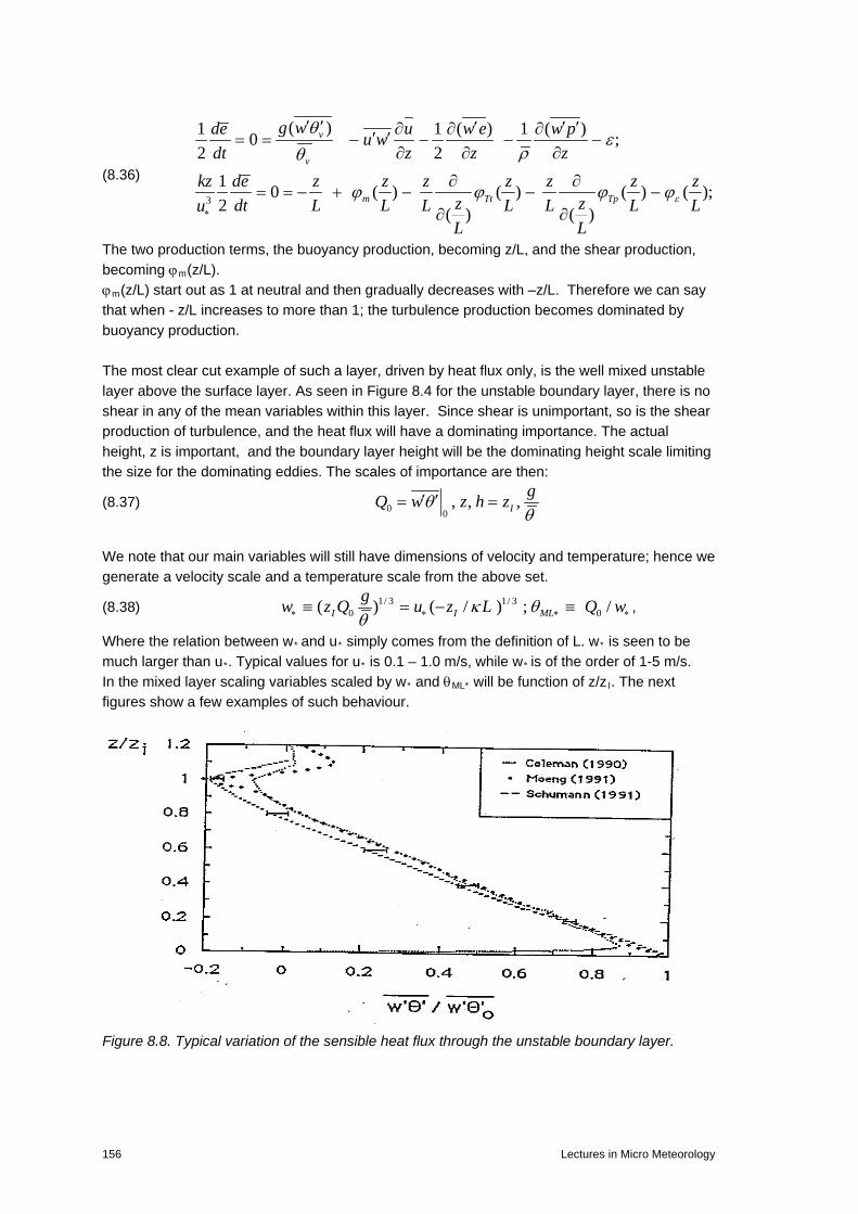
(8.36) 3

( )1 1 ( ) 1 ( )0 ;2 2

1 0 ( ) ( ) ( ) ( );2 ( ) ( )

v

v

m Tt Tp


kz de z z z z z z zz zdt L L L L L L LuL L

ε

θε

ρθ

ϕ ϕ ϕ ϕ∗

′ ′ ′ ′ ′∂ ∂ ∂′ ′= = − − − −∂ ∂ ∂

∂ ∂= = − + − − −

∂ ∂

The two production terms, the buoyancy production, becoming z/L, and the shear production, becoming ϕm(z/L). ϕm(z/L) start out as 1 at neutral and then gradually decreases with –z/L. Therefore we can say that when - z/L increases to more than 1; the turbulence production becomes dominated by buoyancy production. The most clear cut example of such a layer, driven by heat flux only, is the well mixed unstable layer above the surface layer. As seen in Figure 8.4 for the unstable boundary layer, there is no shear in any of the mean variables within this layer. Since shear is unimportant, so is the shear production of turbulence, and the heat flux will have a dominating importance. The actual height, z is important, and the boundary layer height will be the dominating height scale limiting the size for the dominating eddies. The scales of importance are then:

(8.37) 0 0, , ,I

gQ w z h zθθ

′ ′= =

We note that our main variables will still have dimensions of velocity and temperature; hence we generate a velocity scale and a temperature scale from the above set.

(8.38) 1/ 3 1/ 30 0( ) ( / ) ; /I I ML

gw z Q u z L Q wκ θθ∗ ∗ ∗ ∗≡ = − ≡ ,

Where the relation between w* and u* simply comes from the definition of L. w* is seen to be much larger than u*. Typical values for u* is 0.1 – 1.0 m/s, while w* is of the order of 1-5 m/s. In the mixed layer scaling variables scaled by w* and θML* will be function of z/zI. The next figures show a few examples of such behaviour.

Figure 8.8. Typical variation of the sensible heat flux through the unstable boundary layer.


Figure 8.9. Variation of the level of turbulence fluctuations of w and θ through the unstable boundary layer. The different symbols refer to different experiments. The evaluation of the mixed layer scaling laws proceed the same way as for the Monin-Obuchov similarity, namely that data are plotted according to the predicted scaling law, and the validity of the law is evaluated by the quality of the fit between data and model. Note in Figure 8.8 that the heat flux generally decreases throughout the mixed layer. It also changes sign at the top. The sign change at the top means that the heat flux goes from aloft into the boundary layer there. This is consistent with Figure 8.4 showing the unstable boundary layer, where the temperature aloft is larger than the temperature in the boundary layer. The turbulent transport between the boundary layer and the atmosphere aloft is called entrainment. The height variation of the heat flux shows that the mixed layer is not stationary. Recall that we found that for a truly stationary boundary layer the vertical fluxes of all scalars were constant with height. For temperature we have:

(8.39) d wdt zθ θ′ ′∂

= −∂

The fact that the heat decreases with height means that the data have been obtained when the temperature within the unstable boundary layer increases. Indeed, this is also the period when this boundary layer is best defined, as we shall see below. However, first we notice that below the mixed layer we find a matching layer or a free convection layer. This layer is characterised by that it, like the mixed layer is driven by the heat flux, and by convective eddy motion. Unlike the mixed layer it is however not limited by zI because we are down in the surface layer, where z<<zI. Alternatively, this region can be considered a matching region between the surface layer Monin-Obuchov scaling and the mixed

layer scaling, in that it is a region were they should both be true. Examples on the scaling laws applying in the free convection regime are shown in Jensen & Busch (1982). The matching approach is explained in detail in Panofsky (1978) The structure of the unstable boundary layer can be seen also from the point of view of spectra and eddies. In Section 6, the power spectra of turbulence in the surface layer are described, using a combination of data, and Kolmogorov hypotheses and Monin-Obuchov hypotheses. Here it is shown that turbulence spectra by and large are well described by the above set of hypotheses, but that the unstable horizontal components would not adapt to this terminology. The reason is that the low frequencies of the spectra for unstable conditions are more described by the mixed layer scaling than by the surface layer scaling, even in the surface layer. The low frequency part of the spectra can be seen as footprint of the large boundary layer size eddies in Figure 8.4. This is illustrated in the next figure, where the unstable v-spectrum is described as a supposition of a high frequency, small scale part that scales according to the formulations in section 6, and a low frequency part that scales with the mixed layer scaling.

n = fz/U Figure 8.10: The unstable Spectrum of the horizontal lateral component composed by a higher frequency component scaling by the neutral Monin-Obuchov similarity function from section 6 and a lower frequency component scaling with the mixed layer scaling (Højstrup, 1982). In Figure 8.10 the low frequency part of the spectrum scales with w*, while the higher frequency part scales with surface layer scaling. Hence the total spectrum can be formulated a sum of the two:

(8.40)

2 2, , , , , ,

1/ 3*

( ) ( ) ( ) ,

( / ) , , .

u v w u v w i u v w

II i

nS n A n w B n ufz fzwith w z Qg T n nu u

∗ ∗= +

= = =

Where the normalized frequency for the mixed layer, ni is defined for the mixed layer the same way as n is defined in the surface layer. The two forms A(ni) and B(n) represents spectral forms defined in the surface layer, as given in section 6, and the mixed layer respectively. In Figure 6.9, we saw that peak frequency the unstable horizontal spectra could not be described as functions of z/L only, we now see that the reason is the low frequency part, and thereby the


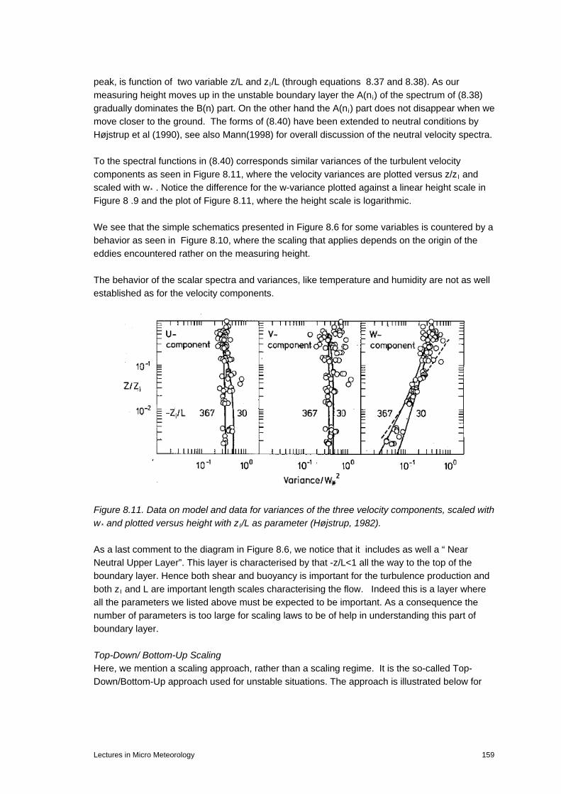
peak, is function of two variable z/L and zI/L (through equations 8.37 and 8.38). As our measuring height moves up in the unstable boundary layer the A(ni) of the spectrum of (8.38) gradually dominates the B(n) part. On the other hand the A(ni) part does not disappear when we move closer to the ground. The forms of (8.40) have been extended to neutral conditions by Højstrup et al (1990), see also Mann(1998) for overall discussion of the neutral velocity spectra. To the spectral functions in (8.40) corresponds similar variances of the turbulent velocity components as seen in Figure 8.11, where the velocity variances are plotted versus z/zI and scaled with w* . Notice the difference for the w-variance plotted against a linear height scale in Figure 8 .9 and the plot of Figure 8.11, where the height scale is logarithmic. We see that the simple schematics presented in Figure 8.6 for some variables is countered by a behavior as seen in Figure 8.10, where the scaling that applies depends on the origin of the eddies encountered rather on the measuring height. The behavior of the scalar spectra and variances, like temperature and humidity are not as well established as for the velocity components.

Figure 8.11. Data on model and data for variances of the three velocity components, scaled with w* and plotted versus height with zI/L as parameter (Højstrup, 1982). As a last comment to the diagram in Figure 8.6, we notice that it includes as well a “ Near Neutral Upper Layer”. This layer is characterised by that -z/L<1 all the way to the top of the boundary layer. Hence both shear and buoyancy is important for the turbulence production and both zI and L are important length scales characterising the flow. Indeed this is a layer where all the parameters we listed above must be expected to be important. As a consequence the number of parameters is too large for scaling laws to be of help in understanding this part of boundary layer.

Top-Down/ Bottom-Up Scaling Here, we mention a scaling approach, rather than a scaling regime. It is the so-called Top- Down/Bottom-Up approach used for unstable situations. The approach is illustrated below for

temperature. We recall that a problem with unstable boundary layers is that K-theory does not work in the middle of the layer becomes the vertical gradients of the variables is very small, due to its “well-mixed” characteristics. A way around this problem is to break the profile down into a sum of two profiles, as indicated, one profile starting above the boundary layer and decreasing down to the ground, an other starting at the surface and decreasing all the way to above the boundary layer. The real profile can then be generated as a weighted sum of the two.

Figure 8.12. Breaking up the temperature gradient into a” top-down” and a” bottom-up” profile. The two profiles each follow their own scaling laws. The bottom up scales with the surface heat flux, it varies as 1-z/zI, while the top-down profiles scales with the heat flux at the top that is heat entrained from above the boundary layer, and it varies with z/zI. An advantage with the approach is that one can include details about the structure of the surface layer at the ground and of the entrainment layer at the boundary layer top. The fluxes through the top of the boundary layer, here of substance C will often be described using the entrainment velocity, we, and a mean gradient.

(8.41) ( ) eh hFlux C w C= ∆

Simple description of the growth of the unstable atmospheric boundary layer. The growth of an unstable boundary layer is depicted on Figure 8.13. The stable night time profile is described by the lapse rate γ, with the surface temperature θ0.(Remember all air temperatures are potential temperatures.) As the sun heats up the ground, the air temperature starts to increase and at a given time is θd. at that time the boundary layer height is h. We assume the whole boundary layer to be well mixed, i.e. at any time with constant potential temperature. From the figure is seen that we have: (8.42) 0 hθ θ γ= +

The relation between the change in boundary layer temperature and the flux divergence is give by:

(8.43) 0 0

1 ( ) (1 2 ) / ,h

d w w w A hdt hθ θ θ θ′ ′ ′ ′ ′ ′= − ≡ +

z I

θ

θ td

θ bu


where A is normally found to be about 0.2, but of course can vary with many things, and be modelled more or less complicated. The A factor is an extremely simple form of the entrainment formulation mentioned above. Inserting the first equation in the second we get:

(8.44) 2

0

1 (1 2 ) / ,2

dh dhh w Adt dt

θ γ′ ′= = +

Denoting:

(8.45) 0

0

( ) (1 2 )t

Q t w A dtθ′ ′ ′= +∫ ,

we can write:

(8.46)

12( )( ) 2 Q th t

γ

=

If the heat flux is constant with time h(t) is seen to increase with the square root of t.

Figure 8.13. Schematics of the growth of an unstable boundary layer driven by the heat flux at the surface and at the top. The equation gives a reasonable description of the growth of the unstable boundary layer as long as the heat flux is increasing or constant with time. After the heat flux decreases and turns negative in the end of the day the boundary layer structure changes, and the above equation does not describe the situation anymore, compare Figure 8.7 that shows how a so called residual layers is slowly forming, consisting of decaying eddies. Indeed what happens at a somewhat more detailed level of description is that the heat flux into the boundary layer creates turbulence and the turbulence is responsible for the growth of the boundary layer, through turbulence diffusion. A more detailed model demands that the turbulence variance equations are included in the process description. Such models have been developed and also give a more comprehensive description of the development of the unstable boundary layer, at the prise of complexity.

θ 0

θ d

h Q h

Q 0

θ

z γ


An example is presented below (Gryning and Batchvarova, 1990).

(8.47) [ ]

220' '

(1 2 ) 2 ( / ) (1 ) swCuh dh w

A h B L g A h B L dtθ

κ γ θ κ γ∗

+ − = + − + −

Where A, B and C are empirical constants, with A being the one already used in (8.43), about 0.2, and B and C about 2.5 and 8 respectively. In spite of its larger complexity it is seen that (8.47) does not contain new parameters relative to the ones already encountered. It is seen that for the growth of a pure mixed layer, u∗ =0, (8.47) reduces to (8.44). It should finally be noted that neither (8.44 nor 8.47) allow for a description of the boundary layer height and the boundary layer structure, when the surface heat flux starts decreasing in the mid-afternoon, and the unstable boundary layer gradually loses its characteristics and starts given room for the night time stable boundary layer. New developments for boundary layer scaling. In (8.44 and 8.47) knowledge about the lapse rate,γ is essential for describing the rise of the boundary layer h. One could therefore think that the thermal stratification of the atmosphere above the could be important for the boundary layer height under all circumstances, especially since it is known that that the atmosphere above the boundary layer is generally stable stratified, and because it seems reasonable that this stratification must influence how easily the turbulent boundary layer can grow into the atmosphere aloft not only for an unstable boundary layer, which we have discussed above. The parameterisation is often formulated in terms of the so called Brunt-Vaisala frequency, N (radians/sec).

(8.48) 1/ 2( ) .gNzθ

θ∂

=∂

The scale N can be combined with a velocity, for example u*, to yield a length scale. The new scale is seen to be independent of the thermal stability and will modify the profiles predicted in this section also for neutral. From N one can generate a length scale as u*/ N, which is seen to have the same form as the boundary layer height, h, in (8.3) and onwards. How these two scales interact and influence the flow is not yet settled completely. Therefore, we shall here not continue to elaborate this new scale, but more point out its possible influence and refer to Esau and Zilitinkevich (2006). However the correction is unlikely to be large for the normal conditions, and a final form for the correction is not yet well established. Example of measurement program in the full boundary layer. In Chapter 6 about the Monin-Obuchov similarity and the surface layer scaling, we showed the set-up of the Kansas 1968 experiment to illustrate the considerations necessary for setting up such a surface layer experiments. Additionally, the experiment has been crucial for the formulation and the validation of this scaling. Similarly, we show in Figure 8.14, the set-up for the Minnesota 1973 experiment that was conducted by the same core-group, also here supplemented by other groups of scientists. The Minnesota 1973 experiment was also crucial for formulation and validation of many of the scaling laws, pertaining to the full boundary layer, as discussed in this chapter, just like the Kansas experiment was for the surface layer expressions in Chapter 6.


Figure 8.14. The experimental configuration for the Minnesota 1973 experiment ( Itzumi and Changhey, 1976) for the whole boundary layer. The lower right hand side set-up corresponds to the Kansas experiment, also denoted CRL in the instrument description. The MRU configuration are all attached to the tether sonde balloon, and described as MRU sensors. The experiment has been central for our description of the unstable and the neutral boundary layer as given in this section. It was less useful for our understanding of the neutral conditions, because the tether sonde had problems for higher wind speeds. (Bush et al, 1979. Drawing : C Kaimal personal communication) Discussion: We have illustrated how scaling laws have been established for many aspects of the atmospheric boundary layer throughout the boundary and for many diverse boundary layer flows. Relative to Figure 8.1. we have now established laws and formulations for the whole boundary layer. Occasionally we have been forced to accept that scaling laws could not be utilised for certain phenomena or only for these phenomena within limited parameter intervals. Also we have been forced to relax some of the basic assumptions behind the derivation of the scaling laws or of the consistency between the different applications of the same scaling formulation. Below is a short summary.


1. The demand to stationarity and horizontal homogeneity was relaxed from the start,

where horizontal pressure gradients had to be accepted for having a simple Barotropic Ekman spiral.

2. Inclusion of a Baroclinic Ekman spiral meant that also horizontal inhomogeneous temperature fields would have to be accepted as a normal part of the atmospheric boundary layer. In section 5 is seen that even very modest horizontal temperature gradients lead to significant deviations from the Barotropic Ekman profile.

3. The mixed layer scaling for the unstable boundary layer is very useful, but typically the boundary layer height and the mean temperature field will now be non-stationary and governed by their own rate equation. However, this non-stationary boundary layer height can be used in connection with mixed layer scaling, and the heat flux typically follows a mixed layer scaling with height, having a gradient reflecting the change in mean temperature. Also strongly stable layers are similarly non-stationary, as the radiational cooling gradually decreases the surface temperature.

4. For unstable conditions power spectra and variances of velocity follows a mixture of surface layer (Monin-Obuchov ) and mixed layer scaling, even well within height intervals, where surface layer formulations govern most of the motion. The reason is that the effect of certain larger eddies can be felt in the surface layer, even when they originate in the mixed layer.

5. Application of many scaling laws is based on the assumption that some parameters are much less important than other parameters, and therefore can be neglected. In practise one will often meet situations, where “much less important” has to be replaced by “slightly less important”, for which reason the less important parameters will show up in the results as well, albeit with less importance.

6. The necessity to include considerations about horizontal inhomogeneity and instationarity is much more important for the description of the flows in the total boundary layer than for flows in the surface layer, as we have seen or remarked repeatedly in this section. After the next section about inhomogeneous boundary layers, we will be able to discuss this statement in more details.


9. Horizontally heterogeneous boundary layers.

So far we have assumed that the boundary layers could be considered horizontally homogeneous, by and large. We shall now leave that assumption and discuss how to handle heterogeneity, a field that is still far from fully l developed.

Considering the natural landscape in the figure 9.1, we obviously have to structure the type of inhomogeneities one can meet, and which often will have to be handled by different models or concepts. A common concept is to consider the influence of a new surface characteristic in terms of a new internal boundary layer growing in to the old one, and reflecting the new surface characteristics. In principle we expect the Geostrophic wind and the general atmosphere over the boundary layer to be unperturbed by the internal boundary layer. However, recall that from the resistance laws we know that the surface flux, the boundary layer height and the Geostrophic wind, with all scalars as well, are interconnected.

Therefore, if an internal boundary layer growths to become a new homogeneous boundary, which will happen if the fetch is large enough, some adjustment will have to happen such that the new boundary layer is in equilibrium with the free atmosphere, as depicted by the resistance laws.

Figure 9.1. Conceptual vision of a heterogeneous surface with associated development of Internal Boundary Layers.

The figure illustrates the response of the atmospheric boundary layer to that the air encounters surfaces with different surface characteristics. Internal boundary layers (IBL) start growing, and each surface have to be characterised by their respective surface characteristics such as terrain elevation, different roughness and surface values of other variables under consideration.


Below, we shall consider different types of internal boundary layers:

1) Change of surface roughness 2) Change of surface heat flux. 3) Change of surface level, hills and ridges, escarpments. 4) Change of turbulent spectrum for changing surface conditions. 5) Additionally, we shall present a selection of characteristic special response to terrain

inhomogenous situations, without going into detailed derivations. 6) In appendix 9.A we shall present a simple derivation of the flow over low hills, both to

illustrate the physical/mathematical principles applied, and to point to practical applications.

Whenever the wind blows over a new surface, theory and data agree that the surface flux changes qualitatively as shown on figure 9.2. The main aspects are that the change in surface fluxes is strongest just at the transition, thereafter the flux relaxes towards a steady level after a few hundred meters. This “steady value” then slowly relaxes to the value it would have if the new surface continued to infinity and the internal boundary layer became a new ”homogenous” boundary layer. The fetch necessary for this final relaxation is usually estimated to be 10-100 km, for neutral stability, shorten for unstable and longer for stable conditions.

Figure 9.2. Qualitative presentation of change in surface fluxes as the air passes over surfaces with different surface characteristics, S1---S5.

The brute force approach to these internal boundary layers is to use a numerical model. Also in the end meteorological numerical models must be able to handle internal boundary layers. Therefore, it is instructive to consider such an approach first

From Section 3 the general equations, we obtain the governing equations for the mean flow in the following form, where we have introduced the special perturbation pressure p’ in addition to the surface Geostrophic wind as well the thermal wind, or baroclinity, from section 5, reflecting larger scale layer averaged horizontal temperature gradient, θL.


(9.1)

2

3

0 3 0 32 1

.1 ( ) ( )

1 ( ) ( ).

1 .

;

j C g jj j

j C g jj j

j jj j

L Lg g g g

C L C L

The three momentum equationsu u pu f v v u ut x x xv v pu f u u v ut x x xw w pu w ut x x x

g gu u x v v xf x f x

The continui

ρ

ρ

ρ

θ θθ θ

′∂ ∂ ∂ ∂ ′ ′+ = − − − −∂ ∂ ∂ ∂

′∂ ∂ ∂ ∂ ′ ′+ = − + − + −∂ ∂ ∂ ∂

′∂ ∂ ∂ ∂ ′ ′+ = − −∂ ∂ ∂ ∂

∂ ∂= − ⋅ = + ⋅

∂ ∂

:

0;

:

( ) ; ( );

i

i

j j j jj j j j

ty equationux

The scalar equationsq qu u u u q

t x x t x xθ θ θ

∂=

∂

∂ ∂ ∂ ∂ ∂ ∂′ ′ ′ ′+ = − + = −∂ ∂ ∂ ∂ ∂ ∂

In these equations we have already simplified somewhat. However, we have introduced the perturbation pressure, which will be essential to describe the flow around hills and other changes in surface elevation and will appear in general when changing surface characteristics introduces abrupt changes in wind speed. They are assumed of such small scale that they do not contribute directly to the larger scale features, like the Geostrophic wind. Also, we have introduced the changes of the Geostrophic Wind with height due to the larger scale horizontal temperature gradient, since the possibility of baroclinity (see section 5) must be considered for heterogeneous situations. θL means that the temperature must be layer averaged (0-x3). Especially at coastal areas baroclinity can be important, due to the very different heat capacity of a land and an ocean surface.

To simplify further we now assume that the change takes place along an infinite line parallel with the y-axis. The wind close to the surface is coming in along the x-direction. Indeed, we do not need the last assumption, because for an infinite line of change along the y-direction, there can be no derivatives along that direction.

Also that the changes do not involve terrain levels and that the pressure perturbation can be neglected (For roughness changes that is true just a short distance away from the line of change). Further neglect baroclinity and assume stationarity, and that the vertical flux divergences are still much larger than the horizontal ones. (Again that can be shown to a good approximation).


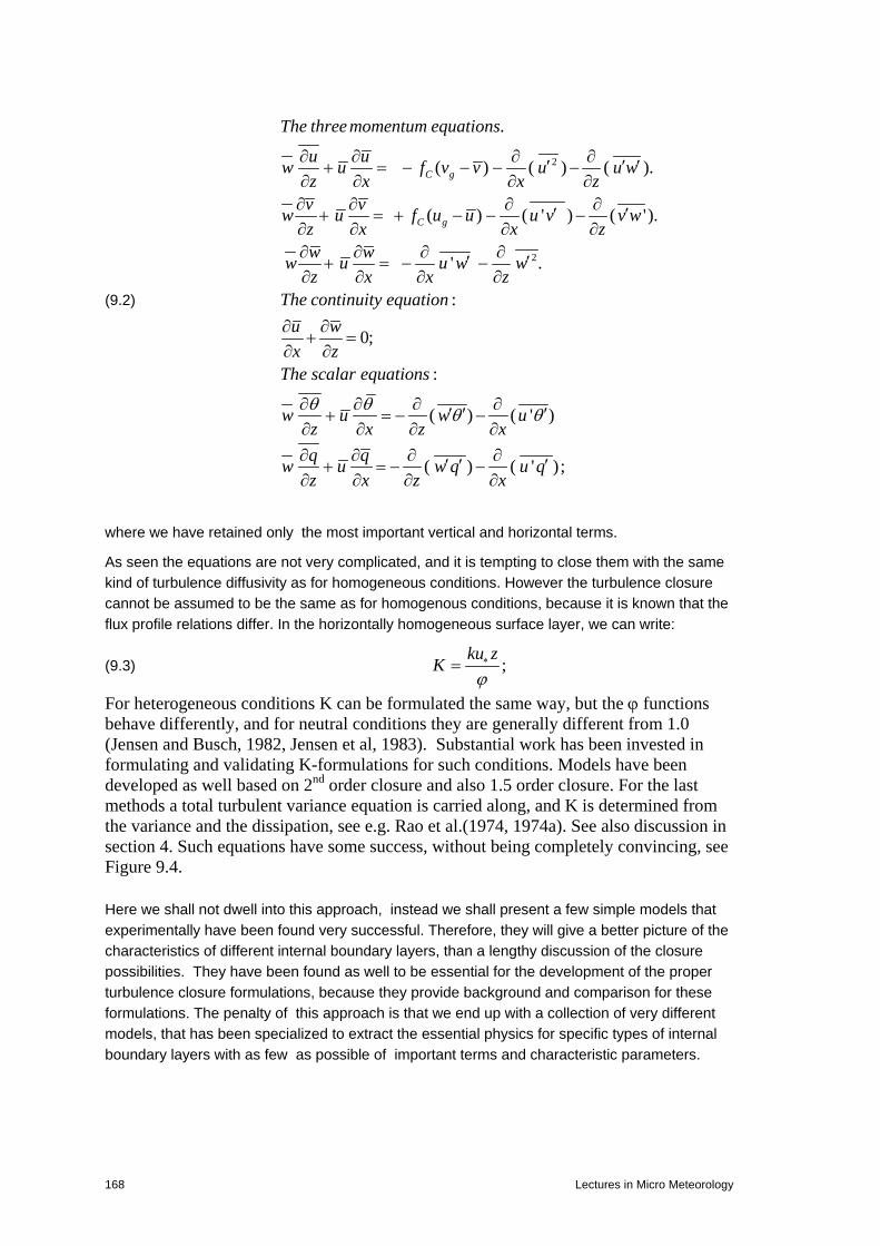
(9.2)

2

2

.

( ) ( ) ( ).

( ) ( ' ) ( ').

' .

:

0;

:

C g

C g

The three momentum equations

u uw u f v v u u wz x x zv vw u f u u u v v wz x x zw ww u u w wz x x z

The continuity equationu wx z


w uzθ θ

∂ ∂ ∂ ∂′ ′ ′+ = − − − −∂ ∂ ∂ ∂∂ ∂ ∂ ∂′ ′+ = + − − −∂ ∂ ∂ ∂∂ ∂ ∂ ∂′ ′+ = − −∂ ∂ ∂ ∂

∂ ∂+ =

∂ ∂

∂ ∂+

∂ ∂( ) ( ' )

( ) ( ' ) ;

w ux z x

q qw u w q u qz x z x

θ θ∂ ∂′ ′ ′= − −∂ ∂

∂ ∂ ∂ ∂′ ′ ′+ = − −∂ ∂ ∂ ∂

where we have retained only the most important vertical and horizontal terms.

As seen the equations are not very complicated, and it is tempting to close them with the same kind of turbulence diffusivity as for homogeneous conditions. However the turbulence closure cannot be assumed to be the same as for homogenous conditions, because it is known that the flux profile relations differ. In the horizontally homogeneous surface layer, we can write:

(9.3) ;ku z

Kϕ∗=

For heterogeneous conditions K can be formulated the same way, but the ϕ functions behave differently, and for neutral conditions they are generally different from 1.0 (Jensen and Busch, 1982, Jensen et al, 1983). Substantial work has been invested in formulating and validating K-formulations for such conditions. Models have been developed as well based on 2nd order closure and also 1.5 order closure. For the last methods a total turbulent variance equation is carried along, and K is determined from the variance and the dissipation, see e.g. Rao et al.(1974, 1974a). See also discussion in section 4. Such equations have some success, without being completely convincing, see Figure 9.4. Here we shall not dwell into this approach, instead we shall present a few simple models that experimentally have been found very successful. Therefore, they will give a better picture of the characteristics of different internal boundary layers, than a lengthy discussion of the closure possibilities. They have been found as well to be essential for the development of the proper turbulence closure formulations, because they provide background and comparison for these formulations. The penalty of this approach is that we end up with a collection of very different models, that has been specialized to extract the essential physics for specific types of internal boundary layers with as few as possible of important terms and characteristic parameters.


Neutral internal boundary layers originating from an abrupt change of terrain roughness, surface layer formulation. The situation is depicted on figure 9.3. The influence of the new surface is growing through turbulence diffusion in an internal boundary layer.

(9.4) 1 0 0( ) wdh hu h A Audt x

σ ∗∂

= = =∂

,

where we associate the growth rate with one of the two velocities associated with vertical diffusion , w and u∗. Subscript 0 indicates that we are considering surface values. It is worth noting that for heterogeneous boundary layers, we know that the constant flux layer approximation is not valid. Hence, we must be careful about specifying the height at which the turbulence quantities are estimated. In the surface layer σw and u∗ are proportional to each other, so for the time being, we settle on u∗. We can now write the growth rate as:

(9.5) 0

0

.( ) ln( )

Audh Ahdx u hz

κ∗= =

where it is assumed that the logarithmic profile scales with the surface stress, although we must assume that also in the surface layer the stress cannot be constant with height close a roughness transition.

Figure 9.3. Description of the structure of the internal boundary, of height h, due to a step change in terrain roughness . Rule of thumb h~ 0.1 x.

Equation (9.5) integrates as follows:

(9.6) 0 0 0

0 0 0

1 ln( ) , :

( 1) (ln( ) 1) 1.

x h

z z

hdx dh orA z

x h hCz z z

κ′

′ ′=

− = − +

∫ ∫

where all the 1’es are relevant only very close to the transition. C is an empirical constant (= Aκ) approximately equal to 0.9. Overall the formula depicts that h is growing somewhat slower than x, about as x0.7. An often used simplistic approximation is h~ x/10.

The physical significance of the exact height of the internal boundary layer, as depicted above, is kind of difficult to evaluate, but we can now determine the ratio between the surface stresses


by matching the up-stream and down-stream profile in h(x). The down-stream profile is determined by that it matches the up-stream value in h(x) and passes through (u,z) = (0, z02), see figure 9.3:

(9.7)

1 21

1 2

02 02

01 01 02 012

1

02 02 02 02

( ) ln( ) ln( )

ln( ) ln( ) ln1 1 ;

ln( ) ln( ) ln( ) ln( )

o o

u uh hu hk z k z

z zh hz z z zu Mh h h hu

z z z z

∗ ∗

∗

∗

= = ⇒

= = = + ≡ +

The ratio between the two surface stresses is a very well defined quantity to measure, and such measurements for short fetches show the model accurately to predict this ratio. From comparing with data, one finds C ≈ 0.9. An example of such data model inter-comparison is shown in the next figure, where this simple model is shown as well to perform better than a second order closure model by Rao et al. (1974), especially for the rough-to-smooth transition. In the figure the open symbols correspond to the model described here, with two different values of C. From the formula and the measurements it is seen that surface stress ratio first shows a large excursion with a sign given the by logarithm of the z0-ratio. For longer fetches the rate of change reduces strongly. The logarithm ratio between the two roughness lengths is denoted M in (9.7), and it is as seen a rational way of describing the magnitude of a roughness change.

Figure 9.4. Comparison between surface stress measurements and different model predictions, the IBL model of (9.7), and the second order closure model of Rao et al, (1974 for smooth- to- rough and for rough-to- smooth transitions. The data (points) are from Bradley (1968. The solid curves are from Rao et al.(1974). The triangles and circles correspond to C equal to 1.0 and 0.5 respectively.(Hedegaard and Larsen ,1983).


Additionally, for long fetches the model does not work well in that the ratio of surface stresses goes to 1 for x going towards infinity. For long fetches we expect the conditions to approach the conditions for horizontally homogeneous boundary layers, where the Geostrophic wind, z0 and u* are interlinked through the resistance laws, as shown in (9.8).

(9.8)

2 2 2

12 2 2

0

0

; ;

((ln ) ) ;

arctan( ) tan( /(ln ));

g gC

g

g

uG u v h

f

kG h A Bu z

v harc B Au z

α

∗

∗

= + =

= − +

= = − −

We shall return to this point later when discussing extensions of the model of (9.4).

For measurement height less than the height of the internal boundary layer, we can estimate the wind speed ratio between up-stream and down –stream winds.

(9.9) 02 01 022 2

1 1

01 02 01

ln( ) ln( ) ln( )( )

.( ) ln( ) ln( ) ln( )

z h zz z zu z u

for z hz h zu z u

z z z

∗

∗

= = ≤

As seen this ratio is not as transparent as the surface stress ratio, because it is a balance between two opposing ratios. However, going back to the model figure, it is seen that if z02 > z01 then u2(z)< u1(z) within the entire internal boundary layer, and vice versa.

The velocity ratio predicted by (9.9) is not in according with data. The model of (9.4) yields an excellent description the ratio between up-stream and down-stream surface stress. If one measures the wind profile at any point downstream the roughness change, one finds a profile that is closer to the profile of figure 9.5 below. Here we can see that the formula above will work only for z< h2, while the up-stream profile prevails down to h1 ≈ h/3. In between one must interpolate. The general lesson of this is that internal boundary layers are pretty idealised features, and their actual height will often vary with the parameters, one considers. Note, however that for this case, they all vary proportionally to each other.

Figure 9.5. Principal structure of the wind profile within an internal boundary layer. The outer and inner profiles (thin lines) are matched at z=h, to provide the surface stress. The inner profiles in equilibrium with the surface stress reach until z= h2 . The outer profile remains valid down to z=h1; between h and h2 the profiles are interpolated. The relation between the heights is h1≈ h/3, h2 ≈ 0.1 h (Jensen and Peterson, 1977, Hunt and Simpson, 1982).

One of the important simplifications in the equation for the growth of the internal boundary layer of (9.6) is that it includes one z0, only, but does not distinguish between the two different z0’s that appear in the problem, the upstream or the downstream value. Therefore, one has to consider this problem outside the model derivations: The use of the formula comes with the rule that one must use the largest z0 to determine the growth rate of the IBL height, the arguments being that the larger z0 creates most turbulence, and the growth of the internal boundary layer is controlled by the turbulence of the one of two layers that is the most turbulent. This has indeed been supported by data that shows that the success of the model depends on the use of this additional rule see Fig. 9.4.

The model described above has been quite successful within its somewhat narrow limitations. This could indicate that the physical principles behind the model are robust. Therefore, several efforts have been made to extend its validity.

Extension to large fetches for neutral boundary layers.

From (9.7) is seen that the surface stress ratio relaxes to 1 for fetch going to infinity. This is not consistent with the resistance laws, as given by (9.8), which show that for larger fetches, two different z0’s must correspond to two different values of surface stress for the same Geostrophic wind. Generally the model behaves unrealistic for large fetches, with respect to the surface stress ratio, and because the internal boundary layer height increases with no limits as fetches goes to infinity, and at least extend beyond validity of the surface layer formulations, being basic to the model. An extended model, repairing some of the fallacies, is shown in figure 9.6.

The extended model is based on the same simple idea as used in (9.4)

(9.10) 1 wdh hu Adt x

σ∂≈ ⋅ =

∂


Figure 9.6. Growths of internal boundary layers that growths towards the total boundary layer height for long fetches, and where a surface stress ratio is achieved that is consistent with the predictions of the resistance laws as given in (9.8) ( Larsen et al.,1982, Sempreviva et al, 1989).

. But both σw and u is now given by expressions that are valid throughout the total boundary layer (Wyngaard, 1982):

(9.11)

20

0 0

0

0

0

(1 )

(ln( ) 2 )

:

w w

c

hu u H

u h huz H

uwith H

f

σ σ

κ

∗ ∗

∗

∗

≅ −

= −

=

,

where we have introduced the scale height of the boundary layer, H, and the wind profile throughout the boundary layer, as derived in Section 8. As for the surface layer description, equation 9.10 with (9.11) can fairly easily be integrated to:

(9.12) 0

0 0

1 ((ln 1) ( )) ,1

: ( ) .

hzx h hC Yhz z H

Hh hwith YH H

− = − −−

≈

The resulting model follows the surface layer model for short fetches and converges to the resistance law predictions for large fetches, with changes going on out to fetches of about 100 km, but with extremely small changes occurring between 20 and 100km. It is seen that the model starts out as a surface layer model for small fetches, and then gradually changes and approach the large fetch solutions. The matching relations involve the profiles of (9.11) rather than just the logarithmic profiles. It is seen from Fig. 9.6 how the matching characteristics depend on if the IBL growth within the upwind boundary layer or directly against the free


atmosphere. In the latter case the cross-isobaric angle also starts approaching the angle for the new equilibrium boundary layer for x→ ∞. See Figure 9.7

The simplistic way of phrasing the models of internal boundary layers (IBL) after a step change is to say that the height of the IBL grows as between x/10 and x/100, dependent on the parameter used to characterize the IBL. This can be turned in two ways. When measuring from a mast at height, z, it means that surface changes closer than about 10z cannot be seen in the data. On the other hand, if one wants to use the resistance laws in section 8 with a characteristic roughness together with the wind at z = 1 km, it means that this roughness must be characteristic for an area with a width between 10 and 100 km.

Figure 9.7. Behaviour of the full boundary layer large fetch model, taken from Hedegaard and Larsen (1983) Extension to changing vertical velocity In the formulations above, it has been assumed that the average vertical velocity remains zero or insignificant. This is not consistent with (9.2), where the continuity equation links changes in <w(x,z)> to changes in <u(x,z)>, and changes in <u(x,z)> are well established, and is one of the key outputs of the models discussed. A simple approach includes <w> iteratively by considering a modification of (9.4).

(9.13) 0( ) ( )hu h Au w hx ∗

∂= +

∂

From this equation one can determine <u(x,z)> as described above, followed by estimation of <w(h,z)>.

(9.14) 0

( , )0, : ( )h

z

u w u z xor w hx z x∂ ∂ ∂

+ = = −∂ ∂ ∂∫

Generally, the wind speed is decreasing for smooth to rough transitions, and increasing for rough to smooth transitions. The correction will therefore introduce an asymmetry in growth rate for the internal boundary layer in the two situations. Obviously it will be most important for shorter fetches, where the change of u is strong and h is large enough for the integral in (9.14) to be significant. The continuity equation is routinely included in numerical models of internal boundary layers, to include the effect changes in vertical velocity from the change in horizontal velocity.

Extension to non-neutral conditions Obviously, there are situations where the thermal stability of the flow is of importance for its response to change of terrain roughness. The same rule is extended to situations where stability plays a role in one or the two of the boundary layers considered. Let us reconsider the growth of the internal boundary layer for non –neutral conditions, corresponding to (9.10), we can somewhat simplistic and naively write:

(9.15) 1

0

( / ),

( ) ln( ) ( )

w wA A k f h Ldhh hdx u hz L

σ

ψ

⋅= =

−

where we have added the stability corrections to both the profile expression and σw/u*0. These functions are very different for stable and unstable situations. The forms, defined in Section 6, are:

(9.16) 1/ 3( ) 1.25 0 ( ) 1.25 1.9( ) 0w wz z z z zf for and f forL L L L L

−≈ ≥ ≈ + − ≤

The profile function ψ(z/L) derives from integration of the non-dimensional shear, ϕ(z/L), as discussed in Section6.

(9.17) 1/ 4( ) 1 5 0, ( ) (1 16 ) 0,z z z z z zfor and forL L L L L L

ϕ ϕ −≈ + ≥ ≈ − ≤

From this derives the ψ(z/L):

(9.18) 1( ) 5 0, ( ) ( ( )) 1 0z z z z z zfor and forL L L L L L

ψ ψ ϕ −≈ − ≥ ≈ − ≤

For unstable conditions, the form of ψ(z/L) is actually a very complicated function. The approximation mentioned here is due to Jensen et al (1984).

Considering the functions above, it is seen that the height of the IBL, h, will grow faster for unstable conditions and slower for stable conditions. Indeed, neglecting the fw-functions, Jensen et al. (1984) constructs an approximate solution as:

(9.19) 0(ln( / ) 1 ( )) ( )h hh h z CxL Lψ ϕ− − ≈ ,


which is seen to become equal to (9.6) for neutral stability. For stable and unstable conditions the growth of the IBL is depicted on the figure below:

Fig. 9.7a. Growth of internal boundary layers for different stabilities. Lower blue line is stable, black is neutral and upper red line is unstable

This concept can further be extended by up-stream and down – stream profiles that includes different stability corrections as well as differences in roughness. As seen the integration and matching procedures loose the esthetical simplicity of the pure neutral case, but can in the principle be performed, and the approach does catch the main characteristics of influence of both stability and roughness for the development of internal boundary layers, although there have never been measurements available for really comprehensive inter-comparison between data and theory. As for (9.6), equation (9.19) is derived without specifying which surface characteristic, we must use, as we by definition has two different surfaces with different roughness and probably also different stability. Again, we will have to appeal to the concept of the strongest turbulence, meaning using the z0 and L that yield the strongest turbulence. Here, the concept may be breaking down, because the two parameters may point to in different directions, and may well each dominate at different fetches, since the IBL will start neutral and become more influence by thermal forcing as h/L increases.

Also another inconsistency in the model becomes apparent. For example, given the definition of the Monin-Obuchov length:

(9.20) 3 /L u wθ∗ ′ ′≈ − ,

we can see that it is only for very special distributions of the heat flux that one can imagine an internal boundary layer with systematic changes of u* with a constant characteristic L-value.

As for the large fetch model, it is seen that for short fetches also the thermally influenced model starts out as a neutral - surface layer model. It also appears that the stability and the full boundary layer models can be combined, by including the proper parameterisations, although the quality of such a combined model has not yet been tested.


The growth of a thermal internal boundary layer (TIBL) within a stable upstream boundary layer. When the heat flux is of dominating importance for the development of an internal boundary layer, a different simple model is often used to describe the development of the TIBL, the thermal internal boundary layer. In its simplest form it is an unstable internal boundary layer that growth against a stable boundary layer.

The concept is taken from the growth of the thermal mixed layer from the morning stable layer over a homogeneous plane, as we discussed in Section 8. Indeed our whole treatment will be build of the formalism developed here. We have changed the text slightly. The main change of concept is that the temporal change in Section 8 is now taken as a temporal change with air mass transport time from the boundary between the upstream somewhat stable boundary layer and the TIBL, one can imagine a coast line with a cold sea and a warm land or vice versa, see Figure 9.9.

The growth of an unstable boundary layer is depicted on Figures 9.8 and 9.9. The stable upstream profile is denoted γ, with the surface temperature θ0. As the air moves over the warm surface, it heats up, after a given transport time the temperature is θd, at that time the boundary layer height is h. We assume the whole boundary layer to be well mixed, i.e. at any time the temperature and velocity are constant with height. From (8.40) - (8.45), and Fig. 9.8 is seen that we have:

(9.21) 0 hθ θ γ= +

The relation between the change in boundary layer temperature and the flux divergence across the internal boundary layer is given by, see (9.2):

(9.22) 0 0

' ' 1 ( ) (1 2 ) / ,h

d w w w w A hdt z hθ θ θ θ θ∂ ′ ′ ′ ′ ′ ′= − ≈ − ≡ +

∂

where t is the flying time from the surface change to x = t . A is normally found to be about 0.2, but of course, it can vary with many things. Such variations are seen to be easy to implement into the model.

Inserting the first equation in the second, we obtain:

(9.23) 2

0

1 (1 2 ) / .2

dh dhh w Adt dt

θ γ′ ′= = +

Denoting:

(9.24) 0

0

( / ) (1 2 )t

Q t x u w A dtθ′ ′ ′= = +∫ ,

we can write:

(9.25)

12( )( / ) 2 Q th t x u

γ

= =

If the heat flux is constant with time h(x/) is seen to increase with the square root of x/,. If the heat flux varies, this can easily be taken into (9.24).

Figure 9.8. The principle for growth of a TIBL due to heat input from the top and bottom.

The equation gives a reasonable description of the growth of the unstable internal boundary layer, as long as the heat flux is not decreasing systematically with time. It can be refined considerable including details of the temperature profile and decreasing heat input, as well as the forcing by the wind, also allowing for neutral or even unstable upstream conditions, through a proper inclusion of the dissipation that imposed internal limitations to the growth. In principle the heating can go on as long as the air moves over the warm surface. As a limitation one can mention that this model is difficult to combine with models that explicitly describe the changes in the velocity profile, because the TIBL model is based on that velocity only plays the role of an advection velocity, being constant with height.

The more advanced model presented in (8.47), Gryning ( 2006) on the other hand includes the turbulence created by the shear profiles, in spite of that the explicit velocity included in the model is a constant advection velocity only. Also this equation can be turned to an equation for growth of a TIBL.

(9.26) [ ]

220' '

(1 2 ) 2 ( / ) (1 ) swCuh dh w

A h B L g A h B L dtθ

κ γ θ κ γ∗

+ − = + − + − ,

Now with:

(9.27) dh h h hu udt t x x

∂ ∂ ∂= + ≈∂ ∂ ∂

The model now describes the situation depicted on the Figure 9.9 below. Simplifications may easily be derived: Letting u* and L go to zero, recovers the simple solution of (9.25). For L going to infinity we obtain an equation for the growth of a neutral internal boundary layer against a free atmosphere with a lapse rate of γ :

(9.28) 2

3

( / ) 1/2

h g C huBu xBu

θ γγ∗∗

∂+ = ∂

,

where the second term in the parenthesis is seen to correspond to the same growth rate as in (9.4), which here is seen to correspond to the initial growth, before the first term in the parenthesis starts dominating. The first term reflects the influence on the growth from the turbulence produced within the IBL, The solution for the boundary layer height, when it is dominated by the first term in the parenthesis is found as (Gryning (2006):

(9.29) 1/336( / ) ,

( / )Bu th t x ugγ θ

∗ = =

which is seen to depend on the stratification aloft.


Figure 9.9. Schematic illustration of the change of surface conditions for use of (9.26 and 9.27)

Wind Profiles over a hill. When air ascends a hill, streamlines converge, and the air accelerates. Typical behaviour of the phenomenon is given in the figures 9.10(a-c) below showing profiles of mean speed and turbulence across a low hill, actually we talk about a two dimensional hill, rather a ridge. The figure also shows the pressure and wind perturbations around the hill, showing how a positive pressure perturbation in front of the hill diminish the flow, while a negative perturbation around the crest accelerates the flow, followed again maybe by a deceleration behind the hill.

The theory of this behaviour has mostly been developed for neutral conditions, although extensions to stable condition have been made. The key reference to the area is Jackson and Hunt (1975). Furthermore the slope must generally be considered small, for the theory to apply, and one generally considers the flow in stream line coordinates or simply terrain following coordinates. Figure 9.10 (a-b) illustrate that for larger steepness flow separation with recirculation may occur. In practise one can often go to larger steepness than theoretically predicted without causing separation.

Jackson and Hunt (1975) separate the flow over the hill into three layers. Layers above the height L are undisturbed by the hill. L is a characteristic scale for the width of the hill typically taken as the half of the width at half height, see Figure 9.10a,b,c, where also the height of the hill, h, is given. The layer below z= L is influenced by the pressure perturbations around the hill, retarding the air before and behind the hill and accelerating it the top. The layer closest to the ground is denoted the inner layer and has the height, . In this layer the flow is influenced by the hill surface through turbulence exchange. As usual the wind is forced to zero at the ground. It is a region with large wind shear. In the height interval between and L is the outer layer, which is primarily influenced by the hill from the pressure perturbations. Notice the characteristic aspect of a pressure perturbation, that it impacts on the flow both up-stream and down-stream


of the change, as opposed to the internal boundary layers from roughness and or heat flux changes that primarily influences the downstream flow, and let the up-stream flow unchanged.

Figure 9.10a. Characteristics of neutral flow across a two dimensional hill, showing wind, pressure and turbulence standard deviations (Hunt and Simpson, 1982).

Figure 9.10b. Characteristics of neutral flow across a two dimensional hill, showing wind, pressure and turbulence standard deviations (Hunt and Simpson, 1982). Two depictions


Figure 9.10c Characteristics of flow across a two dimensional hill, with definitions of flow regions and scales (Britter et al, 1981).

From arguments about turbulence diffusion, the thickness of the inner layer is found from:

(9.30) 20ln( / ) 2z k L⋅ ≈ ⋅ ,

where k as usual is the v. Karman constant, because profile relations are involved in the argument. This result is seen to follow from the roughness change model of (9.6), if we consider the height of the modified velocity layer for a characteristic fetch equal to the width of the hill, L, compare eq. (9.6). In practice one finds: ≈ 0.1 L.

Below z ≈ , the logarithmic profile exists in the usual way with equilibrium between surface stress and wind, although just as for the roughness change boundary layer one finds a stronger horizontal variation of stress, than for the horizontally homogeneous boundary layer.

For the flow over the hill, one estimates a speed-up factor, usually denoted ∆S(x,z).

(9.31) ( ) 0S x, z u / u∆ = ∆

It varies across the hill and with height, as seen in figures 9.10 and appendix 9A, and e.g Zeman and Jensen (1987), and in appendix 9A, being slightly negative in front and behind the hill and positive at the top. Within the inner layer, z<, it is however essentially constant with height. It is defined in (9.31), where Δu is the change of u from far upstream to the top of the hill at a fixed height over the local terrain (or rather fixed stream line), normalised by the upstream wind, u0. Within the inner layer at the top of the hill, it can be written:

(9.32) 2

02

0 0

ln ( / )2 ,

ln ( / )L zu h hS

u L Lz∆

∆ = = ≈

where the last approximation is normally used.

As ∆S is constant with height in the inner layer, the profile remains logarithmic, but with enhanced shear given by ∆S. The maximum speed up takes place at the top of the hill, at the top of the inner layer. There is a gradual variation from the reduced wind in front of the hill to the maximum at the top and down to the wind reduction behind the hill. This is illustrated in Figure 9a,b and in appendix 9.A, where we derive the flow over the hill from a simple linear model, applying Fourier decomposition of the hill.

In the outer region the shear decreases, and a simple way to find the wind is to interpolated between the enhanced wind at height, , and the unchanged wind at height L.

Extension of hill effects Below we show a figure depicting the construction of wind profiles above roughness changes, flow over hills and flow over escarpments that can be treated as hills, with the outer scale, L, given by the distance between the terrain change and the observation poin, based on Jensen(1983). The figure illustrates as well how one can combine roughness change and terrain change effects as multiplicative, provided the modifications are “small”. It works by simply multiplying together, the effects on the flow from the individual modifications.

Figure 9.11. Different types of internal boundary layers and their combination (Hedegaard and Larsen, 1982) In the figure IBL heights are denoted δ, and given by the relevant equations in the text (9.6 and 9.30). The solid line shows the profile at position “b” over the terrain.

The theory, summarised above, has been developed for not real a hill but rather a two- dimensional ridge perpendicular to a neutral wind flow. As such it has been found to match data well, see Figure 9.12 from the experiments on the Askervein hill in Scotland, and the modelling by Zeman and Jensen(1987).

Since it is basically a linear theory, it applies as well for the opposite of a low ridge, a shallow valley.


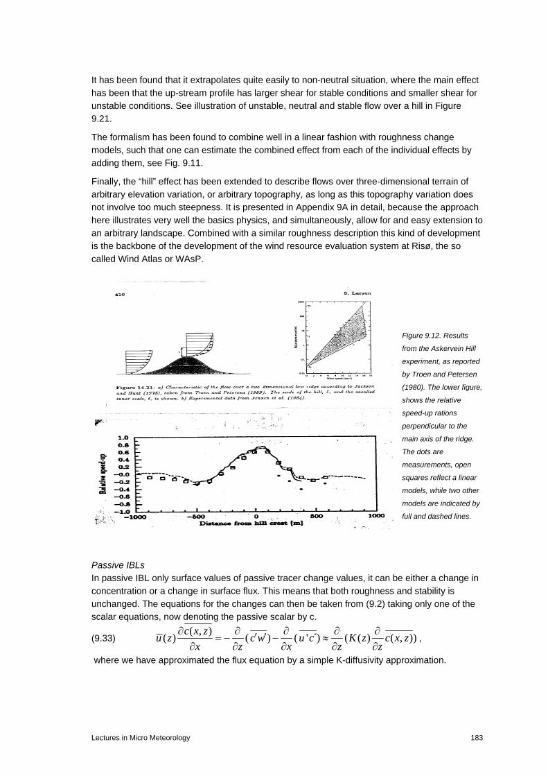
It has been found that it extrapolates quite easily to non-neutral situation, where the main effect has been that the up-stream profile has larger shear for stable conditions and smaller shear for unstable conditions. See illustration of unstable, neutral and stable flow over a hill in Figure 9.21.

The formalism has been found to combine well in a linear fashion with roughness change models, such that one can estimate the combined effect from each of the individual effects by adding them, see Fig. 9.11.

Finally, the “hill” effect has been extended to describe flows over three-dimensional terrain of arbitrary elevation variation, or arbitrary topography, as long as this topography variation does not involve too much steepness. It is presented in Appendix 9A in detail, because the approach here illustrates very well the basics physics, and simultaneously, allow for and easy extension to an arbitrary landscape. Combined with a similar roughness description this kind of development is the backbone of the development of the wind resource evaluation system at Risø, the so called Wind Atlas or WAsP.

Figure 9.12. Results

from the Askervein Hill

experiment, as reported

by Troen and Petersen

(1980). The lower figure,

shows the relative

speed-up rations

perpendicular to the

main axis of the ridge.

The dots are

measurements, open

squares reflect a linear

models, while two other

models are indicated by

full and dashed lines.

Passive IBLs In passive IBL only surface values of passive tracer change values, it can be either a change in concentration or a change in surface flux. This means that both roughness and stability is unchanged. The equations for the changes can then be taken from (9.2) taking only one of the scalar equations, now denoting the passive scalar by c.

(9.33) ( , )( ) ( ) ( ' ) ( ( ) ( , ))c x zu z c w u c K z c x z

x z x z z∂ ∂ ∂ ∂ ∂′ ′= − − ≈∂ ∂ ∂ ∂ ∂

,

where we have approximated the flux equation by a simple K-diffusivity approximation.


It is seen that most of the terms in (9.2) have vanished, since we imagine that we have only step in the surface values of c. The solution of (9.33) can be based on normal surface layer formalisms (Gryning et al, 1983) with

(9.34) 0

( ) (ln ( )), ( ) / ( );cu z z zu z K z u z

z L Lψ κ ϕ

κ∗

∗= − =

The solution of depends on our assumption for the change in surface concentration. If we imagine that the changes take place as a point source, the solution becomes the solution to the dispersion for a surface point source. If we imagine a surface step change along a line perpendicular to the wind speed, we can imagine any such step-change, which involve only c and neither of the other meteorological parameters. Actually, we can reverse the solution to a question about the influence of a surface source change at a given height and a given distance downstream, this normally denoted the foot-print formalisms, used to attribute measured flux or concentrations to given areas up-stream. For good reasons the model in (9.33) corresponds to the description of dispersion from a chimney that we derive in section 10. We can now turn that derivation around and ask where concentration particles measured by a sensor at a given height are ejected from the upstream surface. This is the opposite problem of where does the mass ejected from a source point end up on the surface. The surface origin (the foot print) of concentration measured at a given height and location in the terrain will therefore to a large extent look like the surface concentration for a chimney with the same height as the sensor location and with the opposite wind direction. Detailed treatment of the foot prints has become an important issue in the scientific literature, and the foot print depends on the terrain, stability and not least if fluxes or concentrations are discussed. Foot prints are as well of importance, when fluxes are measured over heterogeneous terrain, where it become important to document what part of the terrain the fluxes refer to, see Horst and Weil (1983) for more details. A typical foot-print form is illustrated in Figure 9.13. It is seen also to be a typical shape for the ground concentration for the elevated chimney plumes in Section 10. As expected areas too close to the mast cannot influence the sensor at the given height, since the tracer will not be able to diffuse to the sensor height from these areas. On the other hand, tracers originating from far away will be highly diluted when they reach the sensor. Unfortunately, even the very simple model of (9.33and 9.34) cannot be solved analytically, but fairly simple by a digital technique, Gryning et al.(1983).

Upwind distance

Flux

per

leng

th u

nit

Figure 9.13. Foot-print for a measured concentration or flux at a given height. The distance between the measuring point at height h and the start of the foot-print is found from σz(x) = h, where σz(x) is the vertical spread of the plume from Section 10.b


Approaches to multiple IBLs, brute force and blending heights. As seen in Figure 1, the real atmospheric boundary layer can be seen as composed of a large multitude of different and overlapping internal boundary layers. Basically, two approaches exist to handle this: 1) applying the individual changes by the models and build the resulting effects by multiplying the effects of the individual models, 2) using the so-called blending height approach. The first approach is used in the Wind Atlas (Troen and Petersen, 1980), where especially the abrupt changes in surface stress near the terrain change is very important to obtain the reliable estimates of the wind speed that is necessary to estimate the wind power resource at a given site.

Figure 9.14a. Introduction of multiple IBL’s to describe the flow across a real landscape (Hedegaard and Larsen, 1982). An alternative approach is to introduce a blending height, where the effects of individual bits of individual of terrain has been lost, or is blended together. The actual blending height formulation of course will have to dependent on the actual form and scales of terrain features. An example is shown in Figure 9.14 for an urban boundary layer. A rough estimate of the blending height can be obtained from diffusion arguments, see section 10:

(9.35) '2

22 ( )b cwh Lu

≈ ,

Where Lc is the characteristic horizontal length scale for surface inhomogeneity (Mahrt, 1996).

Figure 9.14b Individual IBL’s and their merging at a blending height within the total planetary boundary layer (Gryning,2006)


Above the blending height the profile flux relations can be written as:

(9.36) 0

( ) ln( ) ( )eff

eff eff

u z zu zz L

ψκ∗

= −

,

Where the effective values for z0, u* and L have to be derived from detailed considerations about the blending height. Here different authors use different blending heights. Wieringa (1976) and Claussen (1991) refer a height related to the height of the roughness element, while Mason (1988); Wood and Mason (1991) and Mahrt (1996) prefer a height related to the horizontal scale for the roughness changes and the same upward diffusion rate as used in the step change model. The apparent simplicity of (9.36) is achieved at the prize of fairly complicated sub-models describing how one can compute the effective values of z0, u* and L from the surface structure and the flow conditions (Hasager and Jensen, 1998). The discussion above has been concentrated on the response of the boundary layer to inhomogeneous surface conditions. As a note of caution, it should be pointed out that heterogeneity in the boundary layer might be due to other reasons as well. For example, slowly developing synoptic systems and cloud systems will introduce inhomogenity that is originally independent of the surface conditions although the surface might be influenced by for example clouds changing the radiation conditions at the surface.

Turbulence changes within an IBL.

Change of turbulent spectrum for changing surface conditions.

Until now we have discussed the change in mean profiles and the surface fluxes that scale the mean profiles for internal boundary layers. We shall now discuss the changes in the turbulence variances and power spectra. Since different scales of the turbulence are modified differently, it is most rational to consider the modifications of the turbulence spectra. Recall, we considered and rejected using the transport equations (9.1) to derive the change in mean flow within the internal boundary layer. Similarly we shall avoid using the transport equations for fluxes and variances, although, we have these equations available from sections 4 and 6, also they will show quite complicated to use. Instead we shall use some simple semi-empirical models based on spectra, which build conveniently on to our simple IBL models for the mean flow and fluxes.

As for the mean flow considerations we start with changes in surface roughness, and or heat flux. We will consider the change in turbulence, and turbulence spectra. We notice that after a surface change, there will be a local turbulence production, u∗

2dU/dz, within the new IBL that will first be close to the surface and then increase to greater heights, and thereby larger wavelengths, as the IBL grows, because we have seen that this shear production mainly injects energy at eddies with a wavelength λ=z (= 2π/k1, where k1 is the wave number along the x-direction, see discussion in section 2). This local turbulence will gradually replace the turbulence being advected from upstream. Following Højstrup (1981), Panofsky et al.(1982), we consider the spectral modification to follow a first order system:

(9.37) 1 1 1 1 1( ) / ( ( ) ( )) / ( )dS k dt S k S k kτ= − ,


S1 (k1) is the downstream equilibrium spectrum,τ(k1) is an eddy lifetime that depends on the eddy scale, described by k1. For eddies in the inertial sub-range standard dimensional reasoning results in:

(9.38) 1/3 2/31 1( )k kτ ε − −≈

For eddies outside the inertial sub-range, Panofsky proposes to use

(9.39) 11 1( ) ( )uk kτ σ −≈

While Højstrup (1981) proposes ( k1S(k1))½ instead of σu, when focused on unstable conditions, while Mann(1994) assumes (9.38) for all conditions. The eddy lifetime is seen to increase with eddy size for both (9.38) and (9.39), as well as for the assumption of Højstrup (1981). The main difference between the expressions is the rate of increase with eddy size.

Assuming a constant advection velocity, U, with x= Ut, equation (9.36) is easily solved to:

(9.40) 1 1 1 1 1 0 1 1( ) ( ) ( ( ) ( )) exp( / ( ))S k S k S k S k x U kτ− = − − , Where S0 is the upstream spectrum that is also the spectrum above the internal boundary layer, and x=0 is coordinate of the terrain change, S1/S0 is the ratio between the equilibrium spectra upstream and downstream. We follow with an illustration from Højstrup(1981) in Figure 9.15. Equation (9.40) is used to model the transition. Since it is an unstable situation the modifications of u∗ and U are modelled by used of (9.19), while the equilibrium spectra are described as given in (8.40). To understand the behaviour of the spectra in Figure 9.15, we reformulate (9.40) and (9.38) in terms of the normalised frequency, n= k1z/2π =z/λ. (9.41) 1 1 0( ) ( ) ( ( ) ( )) exp( / ( / ))nS n nS n nS n nS n x U n zτ− = − −

(9.42) 1/3 2/3 2/3( )n z nτ ε − −≈

From these equation is seen that in a n-system, the highest frequencies are getting modified first, and the frequency interval that are modified by the new surface becomes wider the lower is the measuring height. This means, that the model is consistent with the idea ,that within the inner layer, see Figure 9.5, the turbulence is in equilibrium with the mean flow, as if the situation was horizontally homogeneous. Outside the IBL, the spectrum is assumed to be equal to the upstream form, denoted nS0(n) in the equations above, the model does not include any interpolation forms. The model also contains other strong simplifications, e.g. that the modified spectrum form must be within the IBL, an argument meaning that z<h, in spite of that this is not explicitly formulated within the model itself, just as for the wind speed prediction in (9.9). Additionally, it is not quite clear how the spectrum behave for z larger that the inner layer height and smaller that the matching height, for h2<z<h in Figure 9.5. Turbulence spectra for flow over hills.

Also for flow over hills the eddy time scale of (9.38) is important to characterise the turbulence modification. As for the surface flux modification above, we will consider the spectra, because different scales modifies differently. We shall follow Frank (1981), who has tried to summarise the work of several authors in terms of the spectral modification through a transfer function G(n= fz/U = z/λ), such that (9.43) 0( ) ( ) ( )a aS n G n S n= ,

n= fz/U Figure 9.15. Model spectra compared to data for a water-land transition from (Højstrup, 1991). The fetch is 53 m from the transition, and the measurement height is 1,2,3 and 5 meter. The height of the boundary layer, ZI=1000 m. At 5 meter only the very high frequency part of the spectrum are affected by the boundary layer change, while at the bottom a wider frequency range is influenced. , Where S0(n) is again the upstream spectrum for horizontally homogenous conditions, Sa the deformed spectrum above the hill, both measured at the same height above the local ground level, or more precisely along the same trajectory .The forms are illustrated for the u- spectrum in Figure 9.16. The form of G(n) depends on the type of spectrum considered and on the scales of distortion as well as the (x,z) position. For the largest scales, we have λ>> L ↔ n<< z/L, where L is the half width of the hill, defined in Figures 9.10, and λ the wave length of the turbulence. For this n-interval, eddies can be considered quasi-stationary, while they move across the hill. Hence the amplitude is amplified by the same ∆𝑆 amplification one finds for the mean wind, see (9.31), therefore, for this n-interval : (9.44) 2( ) ( ) (1 ) , ( ) 1u v wG n G n S G n= = + ∆ ≈ ,

Compare Figure 9.16. The subscripts on the G-functions refer to the velocity components. That Gw is unity is based on measurements (Frank, 1996). It is understood that ∆S(x,z) is a function of both x and z. Close to the ground we find the inner layer (9.30) which is characterised by that the local profile is in equilibrium with the local stress, meaning that we still have a standard logarithmic profile, but with a local stress. Here all the turbulence scales changes such that all turbulence spectra follow the standard forms, scaled by the enhanced stress, meaning that (9.45) 2( ) (1 ) , , , .iG n S i u v w= + ∆ =

Rapid distortion: For transport time across the hill, ∆t = L/U <<τ(k1),where τ is the eddy life time scale, defined in (9.38), the eddies is modified by the changed shear. However, they have not time to interact with each and start the non-linear cascade, we discussed in section 2. They will expand, contract and rotate in the different directions, often leading to a decrease of u’ and enhanced w and v. As eddies are central to the concept, the linearised vorticity equation (not discussed in these notes) is often used for estimating the effects on the velocity components. It can be used in a linearised version because the eddy time scale is exactly a measure of when the non-linear effects of eddy-eddy interaction becomes important. The computations are usually based on isotropic upstream conditions, with correction for non-isotropy (Batchelor and Proudman, 1954, Hunt and Carruthers,1990, Zeman and Jensen, 1987, Britter et al, 1981, Newley, 1985). Based on that the equations are linearised Mann (1994) could extend the solution technique to operate directly on the spectra. The flight time limitation for the rapid distortion can be reduced to a normalized frequency range for their activity can be deduced as follows from (9.38) (9.46) 1/3 2/3

1/t L U kτ ε − −∆ = << ≈

Inserting standard expression of the logarithmic profile, ε∼u∗3/kz, and k1=2πn/z, equation.

(9.46) can be brought on the following form:

(9.47) 3/20/ ( ln( / ))R R

zn n z z zL

λ<< ≡ ≈ ,

Where nR is an upper limit for rapid distortion. Equation (9.47) shows that the n-frequency interval for rapid distortion expand with height, being characterised by (9.48) / Rz L n n<< << .

The lower limit corresponds to the upper limit for the quasi-stationary regime, see (9.45). For n>nR the eddy time scale is now small compared to the distortion time, non-linear cascade effect start acting, and there is no basis for rapid distortion anymore. Therefore the spectra are unmodified. Also close to the ground, in the inner layer, there is no basis for rapid distortion due to lower winds and stronger shear (not included in the rapid distortion formulations, and (9.44) or (9.45) controls the spectral modification. For the rapid distortion one find the following approximate forms for the G(n) functions (Newley, 1985,Frank, 1996):

(9.49)

21

2

3

4( ) ( ) (1 1/ )35

( ) ( 1)(1 4 / 5 )( ) ( 1)(1 6 / 5 )

u

v

w

G n S R

G n R R SG n R R S

µ

µµ

= − ∆ −

= − − + ∆= − − + ∆

,

Where R = (σu/σw)2upstream, is called the anisotropy ratio for the upstream condition. For truly

isotropic turbulence, all components have the same variance and R=1.The µ i are defined as: µ i = (σ i/σ i upstream)2 , i= u,v,w, for isotropic deformed turbulence. Townsend(1976) and Britter et al (1981) finds the following simple variation for the (unrealistic !) conditions of isotropic turbulence: For i= u,v, w, µ i = (σ i/σ i upstream)2= 1±4/5⋅∆S , where the + pertains to i= w,v, while the – pertains to i=u. The R-factor in (9.49) clearly shows the importance of the non-isotropy of the upstream turbulence, as is pointed out by Zeman and Jensen (1987) from a 2nd order closure model.

z/L < n < nR n = zf/U Figure 9.16. Deformation of the longitudinal velocity spectrum above a hill. The figure shows the transfer function G(n) and the undistorted and distorted spectra , both normalized by the upstream u∗,as well three distortion regimes, delimited by z/L and nR (Frank, 1996) .Note that here and throughout this hill turbulence L means that half-width of the hill. Also the curvature of the streamlines is important for the dynamics of the turbulence modification. Over the hill summit the curvature is convex, resulting in a stabilizing effect and a reduction of the w-component, indeed Zeman and Jensen (1987) find model the modification of the w-component due to streamline curvature, r:

2

2 ' 'w

Cur

UU u w

x rσ∂

≈∂

Assuming that the curvature can be estimated from the hill curvature itself, 1/r ∼ -(d2h/dx2)∼-H/L2, one find a curvature effect, cuGw(n), to be multiplied on to the Gw’s in (9.43).

(9.50) 2 2

2 2 2 20 0 0

' '( ) 1 2 2 / ( ) 1 0.4Cu Cuw

w w

Cur

uu w x LHG n H L S G n S

r Lσσ σ σ

∗∆ ∆− ≈ ≈ − ≈ −∆ ≈ − ∆≈ ≈ → .

Tilting modification. Finally the spectra are modified, because the axes of the large quasi-two dimensional eddies will not be tilted similarly to the mean flow on the up-wind of the hill, therefore there will be a component of the upstream horizontal motion of these big eddies in the direction of w. The tilt correction can be computed by a rotation around the y-axis:

(9.51) 0 0

0 0

cos( ) sin( )sin( ) cos( )

u u ww u w

α αα α

′ ′ ′= +′ ′ ′= − +

Where subscript 0 indicates signal with x in the true horizontal direction, and α is the slope angle. There will be a tilt effect for all components, but since the large scale, low-frequency w-component is small, compared to u and v, the effects will be largest for the w-spectrum and for the uw-Co-spectrum., see Figure 9.17. This figure illustrates the behavior of the spectral modification according to the model discussed above.

Figure 9.17. Spectral modifications from Frank (1996). Upstream (full line) and deformed power and co-spectra 10 m above the surface at the summit of a ridge. The parameters used in additional to the ones mentioned ar R=1.5 (9.46), L* is the Monin Obuchov scale in this text. The tilt angle is denoted α. Additional coefficients, as the ones specifying the limits for the different distortion regimes, are found in the paper. Note that the paper has reversed the f and n on the normalised frequency axis. The resulting combined Ga(n) functions in (9.43) thus depend on the details of the flow, the hill-structure and the (x,z) coordinates of the measuring point. However, we notice that most of the spectral modifications are presented in terms of ∆S(x,z) and hence has a certain generality. Frank (1996) compares the spectral model to result from a number of measurement campaigns for hills and escarpments and finds, what one can call a moderately close match with the


different components of the Ga(n) varying in importance with parameters in question and location (x,z) over terrain. Discussion of the turbulence models. Overall we can say that the models for turbulence for different IBLs are quite simplified, and work better for some quantities than for other, The u-spectrum is reasonably well predicted, but the w- spectrum and the uw-co-spectrum show large variability around the predicted values.. The model for the change in surface flux has the advantage of being simple, while the hill model is quite complex, involving many different components and processes. None of the models should be considered accurate. They also involve a number of numerical coefficients, which we have neglected here, where we are focused on the physical concepts only. The coefficients can be found in the papers, referred to. As a technical aspect should be pointed out, that the use of spectra as function of wave numbers, and normalised frequency strictly speaking is incorrect, since a the turbulence is horizontally inhomogeneous . However, a frequency spectrum can be obtained. The argument about the sensitivity to eddy size is also reasonable and the upstream spectral structure can be considered to follow standard boundary layer forms. Hence, it is convenient to use such a notation also for this inhomogeneous terrain. For comparison with the model uncertainties, we include the conclusion from the review of Panofsky et al.(1982) about the spectral modifications for changing terrain conditions:

“Change in roughness: Spectral densities are affected only within the internal boundary layer, and the inertial subrange spectra follow model spectra for homogenous conditions. For horizontal spectra only the high frequency adjust virtually immediately, low frequencies adjust under the influence of the eddy lifetime (that in general influence all scale of the spectrum, but is dominated by the local stress production for higher frequencies).

Over hills and escarpments. In the inner region for the hill tops, the spectra follow and adjust in the same way to the surface stress. For the horizontal spectra the low frequency components are reduced. Above the inner layer rapid distortion and other processes have to be applied.

The vertical velocity spectra follow generally well the homogenous forms because of the overall suppression of the low frequency part. “

To the comparison of Panofsky et al (1982) one could add that there will often be a mixed hill and surface flux modification involved with many hill flows.

Finally, we can point out that the terrain effects on the wind turbulence has been included in the WAsP –Engineering program developed at DTU-WIND, based on the modelling by Mann (1994,1998) and (WAsP Engineering, 2008)

Examples of different thermally influenced IBL’s

The Polynya, represent probably the largest step changes in surface temperature and heat flux within the atmospheric boundary layer, see Figure 9.18. The Polynyas are persistent free water areas within the Arctic sea ice, occupying only a small fraction of the total area of the arctic seas, but are very significant for the total heat exchange between the Arctic Ocean and the atmosphere.


Figure 9.18 Internal Boundary Layer over a Polynya, with very intense heat flux (Andreas, 1980). Notice the sharp 22°C step change in surface temperature. The opposite of an unstable TIBL (Thermal Internal Boundary Layer) is the stable TIBL, often called SIBL, when warmer air passes over a cold surface, most clearly demonstrated for a cold water surface. Stable TIBLs typically use very long fetches to reach equilibrium, because the air eventually will be cooled by the water, but the surface heat flux, responsible for this cooling, is very small, both because of the stability and because of the small water roughness. Eventually at very long fetches, hundreds of kilometres, the whole IBL is cooled to the water temperature, and the boundary layer becomes neutral. The original water- air temperature difference is now concentrated in an elevated inversion.

Figure 9.19. Stable internal boundary layer (SIBL) over water for small and larger fetches (B. Lange, personal Communication) A short example of a SIBL in the Øresund region is seen on the next figure, where the predicted heat flux between air and water as function of fetch is presented (Melas, 1998).


Figure 9.20. Characterization of the dimensionless heat flux in the growing SIBL, showing the dimensionless heat flux versus the dimensionless fetch over a cold a relatively cold Øresund, see left hand figure (Melas,1998) Importance of the thermal structure of the atmospheric boundary layer for flows over hilly terrain. For moderately non neutral stratifications the thermal structure of the flow modifies the flow over the hill in Figure 9.10 and 9.11, as seen in the figure below.

Figure 9.21. Flow over a hill with unstable (red), neutral(black) and stable(blue) upstream wind profiles. The upstream profile is shown to the left of the hill. The black curve reflects the neutral logarithmic profiles. The solid blue line shows a stable profile, while the broken red line reflects

* landp gz

ρ∂= −

∂

* landp gz

ρ∂= −

∂


an unstable profile. The figure illustrates why stable conditions results in larger speed ups on the top of the hill, than neutral, that in turn yields larger speed up than unstable conditions. Recall that the wind at height L is unchanged, for which reason the larger stable wind gradient will increase the speed up over the hill, if we follow the speed up construction described in connection with Figures 9.10 to 9.12. For larger stable stratifications the thermal structure changes the flow considerably, and may determine if the flow will be able to flow across a hill or will have to flow around it. For flow over hill, with height h, one often uses the Froude number, F, to characterize the flow. The more stable the flow, the smaller is F. The higher the wind speed, U, the larger is F.

Figure 9.22. The effect of the Froude number for flow above and around a hill, from emission height, hs, Reynolds number, Re, (Hunt et al, 1978).

1/ 2 1/ 2( ) ( )

UFroudenumber F Nh

g gN z z

ρ θρ θ

= =

∂ ∂= =∂ ∂


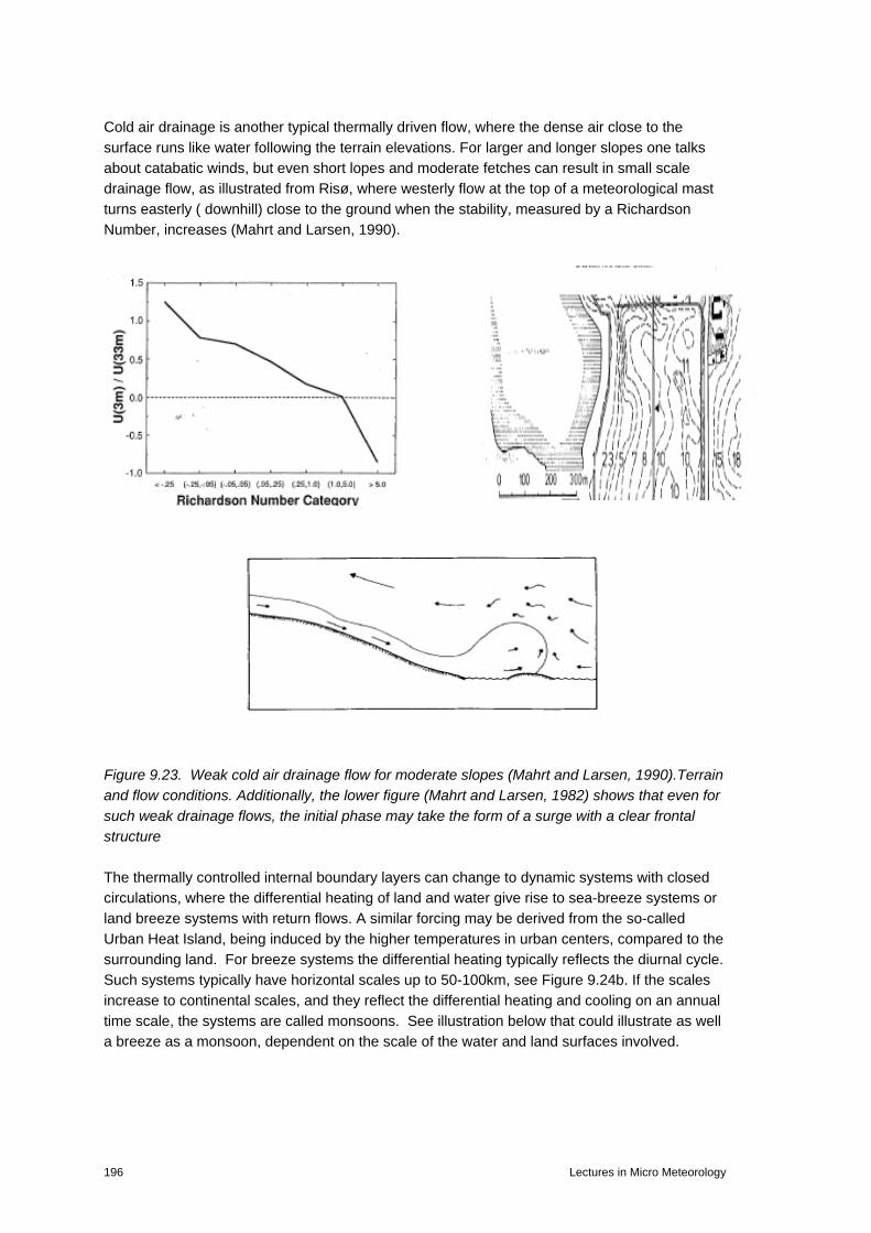
Cold air drainage is another typical thermally driven flow, where the dense air close to the surface runs like water following the terrain elevations. For larger and longer slopes one talks about catabatic winds, but even short lopes and moderate fetches can result in small scale drainage flow, as illustrated from Risø, where westerly flow at the top of a meteorological mast turns easterly ( downhill) close to the ground when the stability, measured by a Richardson Number, increases (Mahrt and Larsen, 1990).

Figure 9.23. Weak cold air drainage flow for moderate slopes (Mahrt and Larsen, 1990).Terrain and flow conditions. Additionally, the lower figure (Mahrt and Larsen, 1982) shows that even for such weak drainage flows, the initial phase may take the form of a surge with a clear frontal structure The thermally controlled internal boundary layers can change to dynamic systems with closed circulations, where the differential heating of land and water give rise to sea-breeze systems or land breeze systems with return flows. A similar forcing may be derived from the so-called Urban Heat Island, being induced by the higher temperatures in urban centers, compared to the surrounding land. For breeze systems the differential heating typically reflects the diurnal cycle. Such systems typically have horizontal scales up to 50-100km, see Figure 9.24b. If the scales increase to continental scales, and they reflect the differential heating and cooling on an annual time scale, the systems are called monsoons. See illustration below that could illustrate as well a breeze as a monsoon, dependent on the scale of the water and land surfaces involved.


Figure 9.24a. A sea breeze system under development. Notice the return flow, the imbedded TIBL, and a between the cool and the warm air. Such fronts occur often between air masses of different characteristics. (Wallace and Hobss, 2006), see also the drainage surge illustration, in Figure 9.23.

Figure 9.24b. Schematic of meso-scale summer and winter monsoon circulation (Miller and Thomson, 1970). Figure 9.25 illustrates a valley wind system that oscillates between cold air drainage and rising air flow along sun-heated slopes.


Figure 9.25. Diurnal cycle of valley winds caused by heating and cooling of the sides of the valley (Hunt and Simpson, 1982) A sea breeze and its return flow can occasionally be seen at chimney plumes, as shown in the picture below from Long Island off New York

. Figure 9.26. Change of flow direction with height at a land-sea breeze situation, illustrated by smoke plumes released at two different heights. Finally, we show a typical experimental set-up to test or at least validate the models for internal boundary layers, here the DUDAMEX experiment on a Dutch island Schiermonnikoog (Højstrup


et al,1982). The main information here is that such experiment by becomes more expensive than similar experiments to test the behavior of homogeneous boundary layers, because measurements has to be done at least in two dimensions, the vertical and along the direction perpendicular to the surface change, here a water front. .

Figure 9.27. Layout for studying change of surface IBL at a coast, from (Højstrup et al, 1982). Compared to the Kansas experiment in Figure 6.1, an additional horizontal dimension has to be monitored. Appendix 9.A. General linear description of neutral stability flow over hills and other orography. We consider a two dimensional hill, a ridge, with a constant velocity u0 approaching the hill perpendicular to the ridge. It is the same hill (ridge) considered in the main text of Section 9, Figure 9.10c. In this appendix we will consider such hills as being described by sinus and cosine functions. Hereby we will see that that the solutions can be applied to arbitrary terrain, as long as the aspect ratio is low enough for linear operations to work. Additionally, the detailed derivation illustrates the simplest physics that can be applied to derive the flow over a hill (Troen et al, 1990, Troen and Petersen, 1989). .


Figure 9A.1. Simplified flow over a two-dimensional hill. Upstream velocity is assumed constant with height. The height of the hill is h, and the width is 2L, measured at h/2. From (3. 83) we have:

(9A.1) 2

3 2

1 2i i ij i ijk j k i j

j i j j

u u upu g u u ut x x x x

δ ε η νρ

∂ ∂ ∂∂ ∂ ′ ′+ = − − − Ω + −∂ ∂ ∂ ∂ ∂

Assuming stationarity, neglecting molecular viscocity and neglecting the Coriolis force, (A1) reduces to:

(9A.2) 31i

j i i jj i j

u pu g u ux x x

δρ

∂ ∂ ∂ ′ ′= − − −∂ ∂ ∂

We now neglect the horizontal turbulence fluxes compared to the vertical and writes:

(9A.3) 2

3 3 2

1 1ij i i i i

j i i

u p pu g u w g K ux x z x z

δ δρ ρ

∂ ∂ ∂ ∂ ∂′ ′= − − − =− − −∂ ∂ ∂ ∂ ∂

Where we have used a constant diffusivity, K. The upstream conditions are defined by uj0 = (u0, 0,0), and p=p0(z) . The wind u0 is a constant and the pressure,. For these conditions, (A3) takes the form:

(9A.4)

20 0 0

0 2

20 0 0 0

0 2

1 , 0 0

1 1, 0

u p uu K orx x zw p w pu g K or gx z z z

ρ

ρ ρ

∂ ∂ ∂= − + =

∂ ∂ ∂

∂ ∂ ∂ ∂= − − + = − −

∂ ∂ ∂ ∂

Which show that we assume the hydrostatic balance to be fulfilled for the chosen upstream conditions, while all other terms are zero. The hill perturbs the flow such that: (9A.5) 0 0, , ( ,0, )j j j jp p p u u u u u w= + = + =


Note that we assume that the perturbed lateral velocity is zero, because out hill is a two-dimensional ridge along the y-direction. Note further that the perturbed variables, ju , p are

different from the turbulence fluctuations that are statistical functions of space and time, while the perturbed flow variables here are deterministic functions of the vertical and the horizontal coordinates around the hill. Equation (9A.3) can now be written:

(9A.6) 2

0 00 3 02

( ) ( )1( ) ( )j jj j i j j

j i

u u p pu u g K u ux x z

δρ

∂ + ∂ + ∂+ = − − − +

∂ ∂ ∂

Keeping only terms of the first order in the perturbed parameters, we can write:

(9A.7)

2

0 2

2

0 2

1 ,

1 ,

u p uu Kx x zw p wu Kx z z

ρ

ρ

∂ ∂ ∂= − +

∂ ∂ ∂

∂ ∂ ∂= − +

∂ ∂ ∂

Where we subtracted the zero terms, as given by (9A.4), and neglected second order terms of the perturbed parameters. (9A.7) is seen to have three unknowns, p , u , w , but includes only two equations. We

introduce the continuity equation as the third equation:

(9A.8)

0 0 0( ) ( ) ( ) 0,

0.

u u v v w w orx y z

u wx z

∂ + ∂ + ∂ ++ + =

∂ ∂ ∂∂ ∂

+ =∂ ∂

As seen, we have a system of partial differential equations. To reduce it to a system of ordinary differential equations, we introduce the Fourier transformed variables, performing the Fourier transforms in the x-direction, where the solutions obviously must be well behaved, due to the limited scale of the hill perturbation. We introduce the Fourier transforms of the variables as follows:

(9A.9)

ˆ ˆ( , ) ( , ) ; ( , ) ( , ) ;

1 ˆ( , ) ( , )

ikx ikx

ikx

u x z u k z e dk w x z w k z e dk

p x z p k z e dkρ

∞ ∞

−∞ −∞

∞

−∞

= ⋅ = ⋅

= ⋅

∫ ∫

∫

,

with corresponding reverse transformations. Here k is the wave number along the x-direction. Inserting (9A.9) in (9A.7) and (9A.8), we obtain the equation for the transformed variables:

(9A.10)

2

0 2

2

0 2

ˆ( , )ˆ ˆ( , ) ( , ) 0,

ˆ ˆ( , ) ( , )ˆ ( , ) 0,

ˆ ( , )ˆ( , ) 0.

u z kiku u z k ikp z k Kz

p z k w z kiku w z k Kdz z

w z kiku z kdz

∂+ − =

∂∂ ∂

+ − =∂

∂+ =


To proceed, we can differentiate the second of these equations with respect to z, and use this and the last equation to eliminate w . Thereafter one differentiates the first of the equations twice and uses this to eliminate p as well. The resulting equation for u becomes:

(9A.11) 4 2

2 0 04 2

ˆ ˆ ˆ( ) 0.iku ikuu uk uz K z K∂ ∂

− + + =∂ ∂

We seek a solution with the height variation of the form: exp(-αz), where α is a complex coefficient, because we expect the perturbation to vanish for large z. Inserting this in (A11), we obtain:

(9A.12) 4 2 2 20 0

2 2 20

( ) 0,

( )( ) 0

iku ikuk k orK K

iku K k

α α

α α

− + + =

− − = With the solutions: α = ±k, and α = ±(iu0k /2K)1/2 = ±(1+i)(u0k/2K)1/2, where we choose the positive k to be systematic. Hence, the solution for u becomes:

(9A.13) ( ) 0 ( )ˆ( , ) exp( (1 ) ),2

abs k z u abs ku z k ae a i zK

−= − − +

We have chosen the minus sign in the exponential functions to ensure that the perturbations disappear for large z. There is one coefficient, a, only, because u = 0 for z =0. Corresponding to (9A.13), we find the expression for w , again using equation (9A.10)

(9A.14) ( ) 01 2

( )ˆ ( , ) exp( (1 ) )2

abs k z u abs kw z k w e w i zK

−= + − +

We now make the connection to the “Flow over Hills” in the main text of this section. Consider a cosine shaped hill, where now a width could be the wavelength, λ =2π/k. Figure 9A.1 illustrate that t the length scale customary used to characterize hills is, L corresponds to about λ/4 that can be taken as L ∼1/k. In the main section was defined as well the inner length scale, , which here must be related to the second exponential , that is:

(9A.15) 0 0

2 2( )

K KLu abs k u

≈ =

To estimate K in a realistic way, we use the surface layer results K = κu∗z ∼ κu∗ , where we have chosen the inner scale as a characteristic z. The inner scale equation now develops as :

(9A.16) 2

2

0 0 0

2 2 2 1,ln( ) 10

u L u L Lor Lu u zκ κ κ∗ ∗= = ≈ ≈

,

Where we have used the logarithmic profile for u0, somewhat inconsistent with the start assumption of a constant u0 in this appendix. It is seen that we arrive to the same approximate relation between L and l , as in the main part of the section (9.30). We now have an intermediate result:


(9A.17)

(1 )

(1 )

1 2

ˆ( , )

ˆ ( , )

z z iL

z z iL

u z k ae ae

w z k w e w e

+− −

+− −

= −

= +

With L = 1/abs(k) and l(k)≅2κ2/ln(l/z0)/abs(k). To solve for the three unknown parameters a,w1,w2, we consider the boundary conditions at the ground, which simply states that the flow has to follow the terrain at zero -level. h(x) u0+ u

w dh/dx = w /( u0+ u ) dh dx Figure 9A.2. The flow following the terrain close to the surface. From figure 9A.2 and (9A.5) is seen that

(9A.18) 0 0( ,0) ( ( ,0)) dh dhw x u u x udx dx

= + ≈

Following the procedures above, we introduce the Fourier transform of h(x)

(9A.19) ˆ ˆ( ) ( ) ; ( ) ( ) ;ikx ikxh x h k e dk h k h x e dx∞ ∞

−

−∞ −∞

= ⋅ = ⋅∫ ∫

Using (9A.9), the boundary condition at (9A.18) can be brought on the form: (9A.20) 0 1 2

ˆˆ ( , 0) ( ) .w k z u ikh k w w= = = +

From (9A.17) we therefore obtain:

(9A.21) (1 )

1 0 1ˆˆ ( , ) ( ( ) )

z z iLw z k w e u ikh k w e

+− −

= + −

From the continuity equation in (9A.6) we get:


(9A.22)

ˆ ( 0, )ˆ ˆ( 0, ) 0; ( 0, ) 0,

ˆ ( 0, ) 0.

w z kiku z k Since iku z kdz

w z kdz

∂ == + = = =

∂ ==

Differentiating (9A.21) we can now solve for w1, to find:

(9A.23) 01

ˆ( )1 (1 )

ikh k uwi L

=− +

We use the continuity equation once more to find the remaining missing coefficient, a, in (9A.17). Assuming the z>L, we can focus on the e-z/L term in the variables

(9A.24)

/ /0

0

ˆˆ ( )( , ) 1ˆ( , ) , :1 (1 )

ˆ( )(1 )

z L z Likh k uw z kiku z k ikae e ordz L i L

h k uaL i

− −∂≈ = − ≈

− +

=− +

Hence we can now write:

(9A.25)

(1 )0

(1 )0

ˆ( )ˆ( , ) ( ),(1 )

ˆ( )ˆ ( , ) ( )1 (1 ) (1 )

z z iL

z z iL

h k uu z k e eL i

ikh k uw z k e eL i L i

+− −

+− −

= −− +

= −− + +

To use (9A.25) to see how the perturbation would look for a real hill, we again consider a cosine hill, defined by:

(9A.26) ( ) ( ( ) ( )h k H k kL Lπ πδ δ= − + +

Hence, ( ) 2 cos xh x HLπ

= , and the perturbation velocity is found from (9A.9, 9A.25, 9A.26):

(9A.27)

(1 )0

(1 )0

0

ˆ( )ˆ( , ) ( , ) ( )(1 )

(( ( ) ( ))( )

(1 )

2 cos( ),

z z iikx ikx L

z z iikx L

z zL

h k uu k z e u k z dk e e e dkL i

H k k uL Le e e dk

L ixu H

L e eL

π πδ δ

π

+∞ ∞ − −

−∞ −∞

+∞ − −

−∞

− −

= = −− +

− + += −

− +

≈ −

∫ ∫

∫

Where we have neglected the i in the (1+i)- terms, which would change the position of the maximum slightly from the top of the cosine. From (9A.27) is seen that the relative over-speeding is largest at the top of the hill and equal to 2H/L This is the same result as in (9.31) in the main part of this section. Here, however we see as well how the over-speeding varies across the hill, from -2H/L to 2H/L. From (9A.25) is seen that the w-perturbation varies not at a cosine, but as a sinus function, with the maximum/minimum w at the middle of the slope.


The height variation is sketched in the next figure, where for increasing z, first e-z/ goes to zero, followed by that e-z/L goes to zero. z L ( , )u x z

Figure 9A.3.The height variations o f the perturbation velocities across hill. The total velocities across the hill is derived by adding the perturbation velocities to the upstream velocity (u0, 0,0). In the derivation we have assumed a constant u0. From the derivation above it is seen that the solutions for the different k-values are uncoupled. Hence, one can choose different u0 for different k-values. For example one can implement a logarithmic wind profile by:

(9A.28) 0 0( ) ln( ( ) / )uu k L k zκ∗≈

Further, it is seen to be it is relatively simple to extend the two-dimensional case discussed above to a three dimensional case, solving the following equations:

(9A.29)

2

0 0 2

2

0 0 2

2

0 0 2

1 ,

1 ,

1

u v p uu v Kx y x zv v p vu v Kx y y zw w p wu v g Kx y z z

ρ

ρ

ρ

∂ ∂ ∂ ∂+ = − +

∂ ∂ ∂ ∂

∂ ∂ ∂ ∂+ = − +

∂ ∂ ∂ ∂

∂ ∂ ∂ ∂+ = − − +

∂ ∂ ∂ ∂

With the variables; (9A.30) 0 0 0( , ,0), ( , , ),u v and u v w together with p and p

,

And the solution method based on the two dimensional Fourier transform:

(9A.31)

ˆ( , ) ( , ) exp( )

ˆ( , ) ( , , ) exp( )

x y x y x y

x y x y x y

h x y h k k ik x ik y dk dk

u x y u k k z ik x ik y dk dk

∞ ∞

−∞ −∞

∞ ∞

−∞ −∞

= +

= +

∫ ∫

∫ ∫


and similarly for the other variables. From this we see that the flow response is related to sinusoidal terrain variations, and since all terrain variations through the Fourier transformation can be considered composed by sinusoidal variations, the solution to any arbitrary landscape and not only hills can be solved by the above systems., provided the hills are not too steep (in theory h/L<<1, in practice h/L<0.4). Hence the starting point for modeling the flow response to a real terrain is to establish a digital version of the elevation h(x,y). The Two dimensional Fourier expansion provides the sinusoidal boundary conditions for solving the 3D flow solution following the outline above. In Figure 12.10 such a map with a superimposed grid system is shown. Note that we have not included stability effects in this summary. They need additional considerations, e.g. Dunkerley et al (2003).

10. Dispersion plumes from chimneys.

In this section we shall focus on the principles behind dispersion from a chimney, both to see the governing principles and to see what it can tell us about the nature of atmospheric turbulence. Turbulent diffusion from stacks Consider Figure10.1 below; the chimney has a source strength, denoted Q [kg/sec.]. Normally one neglects the turbulent diffusion is the x-direction, because the transport in this direction is dominated by the advection by the mean speed. We consider diffusion in the z and y-direction. Actually, we will normally only consider diffusion in one direction and assume the other one to be similar. To simplify further we assume the chimney height to be large enough for us to use a constant diffusivity K = ku∗z ≈ ku∗ h.

Figure.10.1. Dispersion from a chimney, with coordinate system, concentration field, C, wind speed U and diffusivity K. We shall consider the crosswind integrated concentration distribution in the z-direction:

(10.1) ( , ) ( , , )c x z c x y z dy∞

−∞

= ∫

The mean concentration, c(x,z) and the source strength Q is related through:

(10.2) ( , ) ,Q u c x z dz∞

−∞

= ∫

meaning simply that material coming out of the chimney disperses but does not disappear. Note, here is a flux entirely carried by the mean speed. To determine the concentration distribution, we can use the equation for the development of the mean concentration of a passive scalar, see for example. (9.32). As seen, it is basically the same equation for all passive scalars, temperature, humidity and trace concentrations.

z

x

yh

C(x,y,z)

U(z) K


(10.3) jj

j j

u cdc c cudt t x x

′ ′∂∂ ∂= + = −∂ ∂ ∂

We consider only the crosswind integrated concentration distribution c(x,z) and follow the assumption above that K can be considered constant:

(10.4) 2

2

( , ) ( , ) ( , ) .c x z w c c x z c x zu K Kx z z z z

′ ′∂ ∂ ∂ ∂ ∂= − = =

∂ ∂ ∂ ∂ ∂

This equation is solved, using Fourier transform along the z-direction. We employ the transform pair:

(10.5) 1ˆ ˆ( , ) ( , ) ; ( , ) ( , ) ;

2ikz ikzc x z c x k e dk c x k c x z e dz

π

∞ ∞−

−∞ −∞

= =∫ ∫

Inserting these in the equation above we obtain:

(10.6) 2ˆ( , ) ˆ( / ) ( , ) 0;c x k k K u c x kx

∂+ =

∂

which solves to:

(10.7) 2( / )

0ˆ( , ) K u k xc x k c e−=

We can now find c(x,z) by back transforming the above: (10.8)

22

( / )0 0

1ˆ( , ) ( , ) exp( )4( / )4 ( / )

ikz K u k x ikz zc x z c x k e dk c e e dk cK u xK u xπ

∞ ∞−

−∞ −∞

= = = −∫ ∫ ,

where the last transformation takes use of an integral table. With c0 = 1, it is a normalised Gaussian function, meaning that integration over z yields the value c0. As we saw above the concentration and the source strength is related through:

(10.9) 0 0( , ) /Q u c x z dz u c c Q u∞

−∞

= = ⋅ ⇒ =∫

We have now established the crosswind integrated concentration distribution in the z-direction as a Gaussian distribution given by

(10.10) 2

2

1( , ) exp( )2 ( )2 ( ) zz

Q zc x zu xx σπσ

= − ,

with the standard deviation given by:

(10.11) 2zK xu

σ =


It is seen that extension to c(x,y,z) is trivial, so we shall continue to consider only the distribution in the z-direction. It is further possible to integrate equation for more realistic K-profiles with some variation along the z-direction. For a full numerical integration in according with surface layer formulations, see Gryning et al (1983). Lagrangian view of the same problem. To determine the concentration in the smoke plume from the Lagrangian view, we release the smoke at the chimney top as a number of concentration particles. We thereafter sample the particles as they arrive at a distance downstream, and measure the number of packets sampled a given distance from the centreline, N(z), as a measure of the concentration distribution, compare Figure10. 2. Here, we assume that we send the particles off with a time separation large enough for the particles to hit the sampling plane independently of each other. This means that the distribution of N(z) also here becomes a Gaussian distribution.

Figure 10. 2. Particle trajectories for plume dispersion considerations Denoting, the velocity of the particles along their trajectory for w’(t), we can describe the position of the particles by:

(10.12) 0

( ) ( )t

z t w t dt′ ′ ′= ∫

We notice that w’ is a fluctuating velocity with zero average. b The variance of the distribution of particles after flight time t, can be found as:

(10.13)

2

2

0

( ) ( )t

z t w t dt

′ ′ ′= ∫ b

The time (of flight) evolution of the variance can be found from:


(10.14)

2

0 0

2

0 0 0

( ) 2 ( ) ( ) 2 ( ) ( ) 2 ( ) ( )

2 ( ) ( ) 2 ( ) 2 ( ) .

t t

t t t

L L

d dz t z t z t w t w t dt w t w t dtdt dt

w t w t d R d w dτ τ τ τ ρ τ τ

′ ′ ′ ′ ′ ′ ′ ′= = =

′ ′ ′= − = =

∫ ∫

∫ ∫ ∫

Here we have assumed that w(t) is statistically homogenous and stationary, and we have introduced t’ = t-τ ,the auto-covariance function R and its normalised version the autocorrelation function, ρ. Both functions have been given the subscript L for Lagrangian, to remind us that the velocity is measured following a given particle. Notice that for a statistically homogeneous and stationary field, we have:

(10.15) 2 2L Ew w′ ′= ,

where subscript E refers to Eulerian, meaning that the velocity is measured at a fixed point. The reason that the two variance estimates are equal is that for a stationary and homogeneous field all averaging procedures in space and time will approach the same Ensemble average value. We now write the description of the spreading of the plume as:

(10.16) 2 2

0

( ) 2 ( ) .t

z Ld t w ddtσ ρ τ τ′= ∫

The spreading of a smoke plume will therefore depend on the structure of the Lagrangian auto-correlation function. From the figure below, we define a near field- dispersion for small travel times, where ρ ≈ 1, and a far field dispersion for large travel times, when ρ ≈ 0 . Near field: The spreading of the plume can now be written:

(10.17) 2 2 2

0

( ) 2 ( ) 2 .t

z Ld t w d w tdtσ ρ τ τ′ ′= ≈ ⋅∫

or:

(10.18) 2 2 2 2( ) ; ( ) .z zt w t t w tσ σ′ ′= ⋅ = ⋅

Figure 10.3. Langrangian Autocorrelation function


Far field The spreading of the plume can here be written:

(10.19) 2 2 2 2

0 0

( ) 2 ( ) 2 ( ) 2 ,t

z L Ld t w d w d w Tdtσ ρ τ τ ρ τ τ

∞

′ ′ ′= ≈ =∫ ∫

where T is the integral scale for ρL(t), that is the Lagrangian time scale. We now get the standard deviation directly:

(10.20) 2 2 2( ) 2 , ( ) 2z zt w T t t w T tσ σ′ ′= ⋅ =

Comparing with the results derived by the Eulerian picture, using K-theory. (10.21) 2 ( ) 2 , ( ) 2z zt K t t K tσ σ= ⋅ = ,

where we have used that t = x/u. The two methods are seen to yield similar results, for the far field solution, and even allow us a method to estimate a K, which is consistent with our normal way of understanding K . Comparing (10.21) with (10.20) and (10.18)

(10.22) 2

2 2

: .

: .w w w

w w w

Far field K u T u and TNear field K u t u and t

σ σ σ

σ σ σ

′ ′≈ ⋅ = ⋅ ⇒ ≈ ≈ ⋅

′ ′≈ ⋅ = ⋅ ⇒ ≈ ≈ ⋅

However, in the near field the two ways of estimating the plume dispersion do not agree, since the Eulerian estimate predicts that also close to the source the plume disperses as the square root of the flight-time, t½, while the Lagrangian method yields that the plume disperses proportionally to the flight-time. Alternatively one must have a near field K becomes a parameter determined from the plume history (flight time) not only of the turbulence structure, as for the far field. This is contradictory to the concept of diffusivity. We know that the K-diffusivity closure can has problems, and the Lagrangian picture is based on very simple physical concepts (and is confirmed by measurements). Therefore, we believe that the Lagrangian picture reflects the truth, and the results show another example of the failure of K-theory. What happens physically is that the spreading of a plume in the beginning is influenced of the distance to the starting point. First when the change in plume spreading becomes independent of the conditions at the source, in the far-field, we can approximate the dispersion as K-diffusion. Near the source the dispersion processes are still dependent on the release conditions at the source. The K-diffusivity has to be a function of fluid variable and not a function of distance to an arbitrary source. Relation between Lagrangian and Eulerian correlation functions. It is not as simple to measure a Lagrangian correlation function as a Eulerian correlation functions. The relation between the two types of correlation function have however been established both through measurements and through theoretical consideration. At its simplest, one can say that they appears similar in form and the Lagrangian integral time scale is α times longer than the Eulerian intergral time scale, with α ≅ 4. This is in according with that we would expect that the memory of the velocity fluctuations would be larger for Lagrangian fluctuations,


where one follows a specific particle, than for an Eulerian measurements, where the sensor, -so to speak-, measures the velocity of new air particles passing through the sensor every time it measures. The Lagrangian correlation image of the dispersion also means that the transition between near field and far field happens at different travel times for the y-direction than for the z-direction, because integral scales of the correlation functions for the two directions are different and behave differently with height. The reason for this is that within the boundary layer the nearness of the ground suppress large scale signals in the w- components, as we have discussed before in section 2. On a more philosophical note, we notice that we here have been presented for another situation, where the K-diffusivity, which is extensively used in turbulence closures, is not always correct, compare section 4. Practical estimation of atmospheric dispersion. In practise one will translate the dispersion as function of travel time to dispersion as function of distance to the source, using t =x/u.

(10.23)

22

2

2

22 2 2

2

2 2 ,

( )

,

z

ww T t X x Far fieldu

x

ww t x Near fieldu

σ

′ ⋅′ ⋅ ⋅ = ⋅ −

=

′ ⋅′ ⋅ = ⋅ −

It is seen that we can write the spreading of a plume as product of the distance, x, and what we normally call the turbulence intensity, and for the transition between near field and far field, we have the integral scale, X. The turbulence intensity is describable by the similarity function, which we have considered in section 6 and 8 and throughout the literature. Several scaling-formulations are possible, dependent on which scaling regimes that is the most relevant for the situation under consideration.

(10.24)

22 2

1 2 0 1 22 2 2 ( / ) ( / , ) ( / , / ) ( / , / )

( , )

I I I

z

uw w f z L f z L Z or F z z z L F z z z Lu u u

F stability

∗

∗

′ ′⋅ ⋅= ≈ ≈

≈ ∗

In (10.24) the stability is measured by several different formulations, both in surface layer formalism and as mixed layer formulations. The turbulence intensity is a function of stability, however it is estimated in a particular scaling regime, plus some boundary parameters as the roughness and the boundary layer height. Generally this function increases with increasing instability. The behaviour of smoke plumes with stability is illustrated on Figure 10.4 Similar relations pertain to the y-dispersion, as to the, here described, z-dispersion. Description of dispersion for different stabilities is illustrated on the next figure, while the two figures


hereafter show practical sigma -values for y and z, see figure 10.5. these values have trough the time been derived based on an accumulation of dispersion experiments, theoretical considerations and experience with the used values, much the same ways as the consensus roughness diagrams in section 5 have been determined.

Figure 10.4 Chimney plumes for different stabilities, indicated by temperature stratification and the standard (Meteorology and Atomic Energy, AEC, 1968)


Figure 10.5. Typical behaviour of plumes widths as function of distance and atmospheric stability. (Meteorology and Atomic Energy, AEC, 1968)


Additional aspects of plume dispersion. It is worth pointing out that while the plume grows as indicated by the sigma curves discussed above, for an elevated source one will often have a different experience at the ground, where the surface concentration close to the chimney is zero, because the plume has not reached the ground yet. This happens approximately, at a distance, where σz(x) has grown to become equal to the chimney height, h. Around this distance one will one experiences a very fast growth of the surface concentration with x, much as illustrated on Figure 10.6. As illustrated in Figures 10.5 and 10.6, σz(x) is a strong function of stability.

Upwind distance

p

g

. Figure 10.6. Surface concentration downstream of an elevated source. When σz(x) grows from zero at the source to become equal to the chimney height h, the ground concentration reach a maximum, followed by a slower dilution as the plume increases and its concentration therefore decreases. Modern modelling of air pollution dispersion Modern modelling of air-pollution dispersion will normally employ numerical models, either solving (3.82-3.86) simultaneously, or importing meteorological fields, derived from meteorological models and data, and subsequently solving (3.88). As discussed in chapter 4, solution of these equations employs some kind of K-closure, and hence corresponds to the Eulerian concept in this chapter. When point-sources like single stacks are important, plume-models, as the ones considered here, are still used, due to the need of getting the near-field dispersion correct. Even for large scale transport models the near-field Lagrangian characteristics of a point sources can be important because of the importance for the, mostly heat induced, resulting plume height, at which the larger scale advection takes place ( Brandt, 1998). See Figure 10.7.


Figure 10.7. Illustration of a European wide ground modelling across Europe from extensive multiple sources.(Brandt, 1998) Modern plume models are normally formulated in terms of puffs, clouds of particles, which can then be advected by a changing mean wind field. Also combined numerical modelling that allow for important point-sources, where near-field dispersion characteristics is then included. Physically, dispersions from puffs are derived considering the change in distance between pairs of particles, released nearly simultaneously at the source as opposed to the plume dispersion considered here, where the distance between single particles from a centre line is considered. This difference yields a stronger scale dependency for puff dispersion than for the plume dispersion. Additionally the winds moving the individual particles are now correlated, making the statistical treatment more complicated. Therefore, we shall not discuss puff dispersion here, where we have just touched upon dispersion, but we refer to Mikkelsen et al (1984, 1987). A concentration pattern from a European wide dispersion experiment from such models are illustrated on Figure 10.7. Spectral description of plume dispersion. In the above discussions we have used the Lagrangian correlation function to derive the plume dispersion. For illustration we shall summarise the same derivation using Lagrangian spectra for the same derivation. We shall use results from section 2, equation (2.50) to (2.52), with only slight modifications. We can Fourier decompose the Lagrangian vertical velocity, w’(t) in (10.12) as follows:

(10.25) '( ) ( )i tww t e dZω ω

∞

−∞

= ∫

Next we follow (10.12) for estimating z(t):

(10.26) / 2

0 0

sin( / 2)'( ) ( )

/ 2( )( )

ti t

w

ti

wt

w e dZt

d e dZ d tz t ωωτ ωτ ω

ωτ ω τ

∞

−∞

∞

−∞

= = =∫ ∫∫ ∫ ,


where we have performed the τ-integration. Next we square z(t) and average to arrive to:

(10.27) 2

2 2 2

2

( )sin( / 2)( ) ( ) * ( )

/ 2w

z

Stt z t z t w t d

t w

ωωσ ω

ω

∞

−∞

= = ∫ ,

where * denotes complex conjugation as usual, and we have followed the definitions and methodologies described in section2, for creating variances, see (2.35) to (2.53). As discussed in section 2 the sinc2(ωt/2) function acts a low pass filter suppressing frequencies ω >π/t. We can use this to check the near field and far field solutions in (10.17) and (10.30). For the flight time t very small the sinc –function is seen to be unimportant, the normalised spectrum integrates to 1, and we recover (10.18), for the near field spreading. For t large, the sinc-filter reduces the spectrum to its value at ω = 0, and (10.27) takes the form:

(10.28) 2

2 2 2 2 2 2

2

( 0)sin( / 2) 2 2( ) 2

/ 2 2w

z

St Tt w t d w t w Tt

t tw

ωω πσ ω

ω π

∞

−∞

== = =

∫ ,

where we have recovered equation (10.20). We have used (2.38), for the relation between the integral scale and S(0), with the exception of that (10.20) defines T from integration over the positive parts of the correlation function (0, ∞), while we in section 2 define it by integration (-∞, ∞). The 2π/t derives from the integration of the sinc-function. Eulerian- Lagrangian spectral statistics. We shall now change the Langrangian turbulence spectra used (10.27) to Eulerian turbulence spectra. An advantage here is that we can more easily shift between frequency and wave number statistics, using Taylors Hypothesis. Above we discussed that the Lagrangian correlation function could be related to the Eulerian correlation through RL(τ) = RE(τ/α), with α at its simplest around 4. From this we find the corresponding spectral relation:

(10.29) ( )( / )1( ) ( ) ( / ) ( / ) ( )

2 2i i

L L E ES R e d R e d Sωτ ωα τ ααω τ τ τ α τ α α αω

π π− −= = =∫ ∫

Which shows that the Lagrian spectrum relative to the Eulerian one is larger at lower frequencies and lower at higher frequencies, and is consistent with a Lagrangian time scale equals α times the Eulerian one. We now use (10.27), emphasizing the difference between Lagrangian and Eulerian spectra:


(10.30)

2

2 2 2

2

2 2

2 2 2 2

2 2

2 2

2

2 2

( ')sin( ' / 2)( ) ( ) * ( ) '

' / 2

( ' ) ( )sin( ' / 2) sin( / 2 )'

' / 2 / 2

( )sin( / 2 )

/ 2

Lwz

Ew Ew

Ew

Stt z t z t w t d

t w

S St tw t d w t d

t tw w

S kw kxx dk

U kx w

ωωσ ω

ω

α ω α ωω ω αω ω

ω ω α

α

α

∞

−∞

∞ ∞

−∞ −∞

∞

−∞

= =

= = =

=

∫

∫ ∫

∫

Where we have used Taylor hypotheses in two forms: x = U·t, and ω = U·k. From the last equation in (10.30), it is seen that the sinc-function determines which eddies that contribute most to the dispersion , because such eddies are characterised by wave numbers, k, or a wave lengths, λ, with k·x /2α << π or λ ≥ x/α. Therefore, close to the source, with x close to zero, the full w-spectrum contributes to the diffusion, but as the distance to the source increases, the smaller eddies are cut out, and only larger and larger eddies contribute. As x becomes large enough, the dispersion approach the far field mode, as the spectrum approach SEw(0). This is consistent with the analysis in (10.22) showing that the length scale associated with a K- dispersion of a plume, should be of the order of the standard deviation of w times the flight time, in the near field, until it approaches the standard deviation of w times the Lagrangian time scale, in the far field. As we have discussed in section 2 and 6 , Eulerian spectra continue to smaller and smaller frequencies and therefore larger and larger scales, compare Figure 6.10 and 2,23, and especially for the horizontal wind components, responsible for the horizontal plume dispersion, there is considerable energy at the lower frequencies. This means that the simple hypothesis of the spectrum converging towards a S(0), reflecting one and only one characteristic time scale , for small frequencies does often not apply in practise, where the spectrum rather become modified by new processes being responsible for the variability. Also for these practical situations, equation (10.30) continues to apply, as long as we can apply the simple Lagrangian-Eulerian transfer and also apply Taylor’s hypothesis. On the other hand, as the flight time and distance to the source, other aspects of the present model become less realistic, such as the assumed stationarity of wind speed , wind direction and source strength. Therefore, one will today use numerical codes, either in the form of Eulerian diffusion models or Lagrangian puff-models or combinations of such models (Mikkelsen et al, 1987,Brandt, 1998).

. Dispersion experiments from an individual source for different atmospheric conditions, compare Figure 10.4. (T. Mikkelsen, personal communikation)


11. Boundary layer climate, radiation, surface energy balance.

In the earlier section we have derived characteristics of the boundary layer flow and turbulence in terms of its response to different forcing and boundary conditions. We will understand boundary layer climatology as description of the characteristic weather phenomena within the boundary layer at a given location, in response to its peculiar boundary conditions, and the forcing. Different types of boundary conditions have been presented in these earlier sections, and we have seen how these conditions can modify the local meteorological conditions. Therefore, we shall characterize the forcing by the larger scale meteorology, being responsible for bringing different air masses across a location, and the radiational forcing of local cooling and heating of the air. As also the large scale weather is driven by the radiation balance, the importance of this forcing is obvious. Hence, we start discussing the of the radiation balance at the Earth’s surface. Radiation and energy balance at the ground. Some definitions: All bodies with temperature above zero Kelvin emit radiation. A black body emits maximum possible radiation for its temperature. The energy emitted from a body of temperature T0 follows the Stephan – Boltzmann law: (11.1) Energy emitted = ε∙σ∙ T0

4, Where T0 is the surface temperature of the body, σ, the Stephan –Boltzmann constant. σ = 5.67∙10-8 Wm-2K-4 and ε ≤ 1, is denoted the emissivity and being 1 for a black body and less for a normal (grey body). The wavelength distribution of the emitted radiation follows a Planck curve, see Fig. 11.1. For increasing temperature the emission increases strongly, and the Planck curve is shifted towards smaller wavelengths, following Wien’s Displacement Law: (11.2) λmax = 2.88∙10-3 [mK]/ T0 ,

Fig. 11.1. Spectral distribution of energy radiating from the Sun (T= 6000 K), at left hand side, and Earth (T= 300 K), right hand side, considered a black bodies. (Oke, 1985). When a radiation flux of wavelength λ incidents on another body, the response of this other body is characterized by its transmissivity, Ψλ, its reflectivity αλ and its absorptivity, ζλ = ελ, where it can be shown that the absorptivity is the same as the emissivity (denoted Kirchhoff’s law). The relations between these terms are


(11.2) Ψ λ + αλ + ζλ = 1; Strictly speaking this relation is correct only for a specific wavelength, but it holds approximately for wavelength bands as well. For Solar radiation one talks about the reflectivity as α, and it is denoted the albedo. For opaque bodies (Ψ λ =0), the reflectivity and the emissivity are relates as: αλ = 1- ελ . The difference in wave length between solar emission, being of relatively short waves, and the Earths emission being of relatively long wavelength, results in the so-called green house effect, because the transmissivity of Earth’s atmosphere is much larger for the solar radiation, than for the more long wave Earth radiation, see Fig. 11.2

Fig. 11.2. The flux of solar radiation, irradiance, outside the atmosphere and at the sea level. The much larger tramissivity in the visible region versus the lower transmissivity at the longer wavelength region, the infrared is clearly seen.(Oke, 1985) Atmospheric radiation can be discussed either from the perspective of what happens with a specific radiation, or how radiation enters into the energy balance at a certain spot or level. We start considering the Solar irradiance, i.e. the radiation flux reaching the top of the atmosphere. The solar constant, S0, is the power (Wm-2) of the solar radiation reaching a sphere at Earth’ distance from the Sun and outside the Earth’ atmosphere. One has S0= 1370 Wm-2. Figure 11.3 shows such how the Solar irradiance is distributed within the atmosphere. The irradiance outside the atmosphere is taken as 100%. Note that 100% does not necessarily correspond to S0, since it depends on the solar height at the location studied and the averaging time employed.

Fig.11.3. Distribution of the solar irradiance as it reaches the Earth. It is seen that 30% is reflected back to space, 51 % is absorbed by the ground and 19% is absorbed by the atmosphere (Shodor,1996).


In the next figure, Fig. 11.4, we consider the energy balance for certain parts of the Earth system.

Fig. 11.4 Energy balance for various Earth systems, the atmosphere, clouds, the surface. The units are the 100% solar irradiance arriving at the top of the atmosphere in Fig. 11.3. As seen 51 % reach the surface and 19 % reach the atmosphere. The reflected 30% is neglected in this figure. Each system should have balance between gains and losses for the temperature to remain constant (Shodor,1996). Note in Fig. 11.4 that the Earth system lose as much energy by radiation as it receives from space, for the Earth to retain its temperature. The wavelength of the Sun and Earth radiation are different, but the energy is the same for the total Earth system to retain its temperature. In Fig. 11.5 is shown the diurnal cycle of the radiation balance and the resulting surface temperature. It is illustrated how the surface gains heat and temperature during the day due to that the incoming solar radiation dominates the energy losses of the surface. At night the loss terms dominate and the surface temperature decreases, ensuring that the average of the diurnal temperature variation is approximately zero. The variation of the surface temperature will be modified also by advection of air with different temperatures, and by heating and cooling from the ground. Also, the diurnal temperature variation in response to the incoming radiational heating will depend on the characteristics of the surface, such as heat capacity and heat conductivity.

Fig. 11.5. Diurnal variation of the surface energy balance and the associated surface temperature (Shodor, 1996),


A more thorough discussion of the energy balance demands that we consider the system of equations controlling the balance. It is normally written as: (11.3) Q* = K↓+ K↑+L↓+L↑= QH + QE+ ΔQs . Q* is net radiation, and K↓ is incoming short wave radiation. K↑= α K↓is outgoing short wave radiation, α is the surface albedo. L↓ is incoming long-wave radiation, and L↑ is outgoing long-wave radiation = εσΤ4 + (1- ε)L↓, ε is the surface emissivity ,and σ is the Stefan-Boltzmann constant. T is the surface temperature. Above, we noticed that an often used relation between is αλ = 1- ελ, but its application assumes that the same wave length applies on both side of the equation. Here, we will use the albedo, α, in connection with the short wave radiation and the surface emissivity in connection with the long wave radiation. Characteristic Values of albedo and emissivity for different surfaces are shown in Table 11.1 below. Continuing with the non-radiative terms of the energy balance, we have two turbulence flux terms and a heat conduction term. QH = ρ Cp <w’T’> = ρ Cpu*θ* , the sensible heat flux, ρ is the air density, Cp the heat capacity of air at constant pressure, where the air density , ρ, is about 1 kgm-3 and Cp ~ 1010 J∙K-1∙kg-1. The u*θ*-term reflects the Monin-Obuchov- scaling, discussed in section 6. QE = ρ Lv <w’q’> = ρ Lv u*q* , the latent heat flux, Lv the evaporation/condensation heat being approximately equal to 2.45 MJ∙kg-1 , where we have shown the surface layer formulation as well. Similarly to u*θ*, u*q* is defined and discussed in section 6.

The sensible heat flux obviously reflects turbulence heat flux between the surface and the air, while the latent heat flux reflects that the surface can regulate its temperature by evaporating or condensing water. ΔQs is the heat storage per unit time in the surface material ~C dΤ/dt, with C being the heat capacity of the surface, where C depends on the surface characteristics. Here we obviously have to consider that the surface have a certain depth to distribute the heat input or loss. Typical values for C (JK-1m-3) are shown in table 11.2 for characteristic surfaces. It is seen from the figure that wet surfaces have larger heat capacities. Defining the heat conductivity, λ , for the surface, we can trace conduction of ΔQs down into the surface material, through ΔQs = - λ (δT/δz), where ΔQs(z<0) is now considered a function of z. Combining this within the heat conduction equation, we obtain: (11.4) Where, κ = λ/C, is the thermal conductivity. This is the same equation, we use to solve for a dispersion plume from a chimney in section 10. Here we notice that the surface temperature on both annual and diurnal frequencies is related to a sinusoidal, and assume that the surface temperature can be written as : Ts = Tav + δTsin (ωt), where Tav is the average temperature and δT is the surface diurnal temperature amplitude related to the radiation. Inserting and solving (11.4), we find:

(11.5) / 2 sin( / 2 )zs avT T Te t zω κδ ω ω κ−= + − ,

Which illustrates how surface modulation of the temperature propagates downwards, with an amplitude attenuation and a phase change given by the frequency of modulation and the thermal conductivity. Equation (11.5) is illustrated on Figure 11.8. Characteristic radiational parameters are given in table 11.1, 11.2 and 11.3.

2 2

2 2

1 1 ( )sQdT T T T Tdt t C z C z z C z z

λλ κ∂∆∂ ∂ ∂ ∂ ∂= = − = − − = ≡∂ ∂ ∂ ∂ ∂ ∂

Table 11.1 reflectivity and emissivity for different natural surfaces, ε corresponds to long wave radiation, while α reflects shorter wave lengths.(Oke, 1985).

Table 11.2 Heat capacity for different types of surfaces, [Jm-3K-1],(Christen 2004)

Table 11.3 Thermal conductivity for different types of surfaces (Christen, 2004). From the discussions above, it is obvious that the energy balance at the surface will depend on the surface characteristic, and hence can be pretty different for nearby but different surfaces.


This is illustrated in Figure 11.6, showing the diurnal variation of some of the terms in the energy balance for a suburban and a rural Vancouver site, as well as their differences. Figure 11.7 shows the annual variation of the net radiation, Q*, at a rural site in Denmark.

Fig. 11.6. Diurnal variation of some of the terms in the energy balance for a suburban and a rural Vancouver site, as well as their differences. Notice the difference between the latent heatlux of the two sites (Oke, 1985). The notation is as defined above in the text.

Figure 11.7. Annual variation of Total daily net-radiation at an agricultural site in Denmark at 55degr North, 1961-1979. The figure shows both average values and extreme values for the period considered (Larsen and Jensen, 1983). A characteristic behaviour of ground temperature profiles for a land surface versus time for a diurnal variation is shown on Figure 11.8 below.


Figure 11.8 Examples of the diurnal variation of ground temperature profiles for a Pine forest in Germany (Christen, 2004) The local climate The local climate of any sites will depend on the larger scale climate around the site, and on the local energy balance, as discussed above. Also other local features are important however, such as local terrain, thermal and roughness characteristics and wetness of the site, which will influence the wind, the energy balance and temperature and humidity statistics. Larger free water surfaces are able to regulate their temperature because of, additionally to large heat capacity of water, it applies latent heat flux at the surface and enhanced vertical mixing due to waves and turbulence in the inner volume. For salty water this mixing is further enhanced because warm surface water evaporates, and hence becomes heavier due a higher salt concentration. On the other hand cold surface water sinks, because it is heavier than the water below. Therefore, we find that diurnal temperature variations is smaller both on the surface and with smaller penetration into the water mass than for a land surface. For latitude with significant annual periods in the radiation budget (11.5) can still be used now with a suitable annual frequency. For this frequency one generally finds that the temperature changes at water surface and below is closer to those of a land surface. Further one finds that the effective thermal capacity and conductivity of the water will be functions of current and wind speed and buoyancy influencing both evaporation and the internal turbulent mixing in the water boundary layer, just as in the atmospheric boundary layer over the water, but with the added complexity of the importance of salinity for the buoyancy. Obtaining the climate characteristics. Due to the variety of forces behind the climate at a given spot, it is mostly determined empirically from multiyear measurements of the relevant parameters at the point of interest. Therefore many basic climate data are obtained from observations from a measuring station, which can be centred around a meteorological mast as seen in Figure 11.9. A station, like this, must be maintained and serviced for several years to develop a local climatology, formally referring to the exact location of the mast. The strength of such a station


is that it obviously monitors the climate at a certain location, while our ability to extend the results to wider areas depends on the heterogeneity of the surroundings and on our understanding of the micrometeorological characteristics of the data and the site. Some parameters are more local than other. We have seen that the wind quite sensitive to roughness, terrain variation and shelter effects. Surface temperature is being sensitive to the local energy balance, will be sensitive to slopes and orientation of slopes etc, therefore one should always consider the locality of a given record and of a site, where the climate has to be evaluated. Here it is often possible to draw from knowledge about boundary layer meteorology, such as presented in this course. In the measurements depicted in Figure 11.10 there is an effort to cover a larger area with many point measurements, supported by airplanes and satellites. Such a network of measurements are obvious both more expensive and difficult to keep operating but can be used for validation of modelling. However, also here the aggregation of the individual data sets have to include a substantial amount of the micrometeorological understanding and modelling.

Figure 11.9. A typical meteorological mast instrumented with wind, temperature and humidity measurements at several heights. Such a mast will typically be supplemented with measurements of pressure, precipitation, various radiation measurements, and various soil ground measurements, situated on and around the mast structure (A typical wind Risø , DTU-Wind-configuration).


Figure 11.10 Climate measuring program set up to cover an extended area. Finally, we turn to climatology data derived from the so called reanalysis data, which is based on applying many years of the initial meteorological fields used in weather forecast modelling or climate modelling. Here basically all the observations, used to initialize these models, are used to provide a homogenous climate data set covering all the grid point in the models used. The obvious advantages with this method, is that it provides homogenous data with good area coverage, and also provide the climate for a vast suite of meteorological parameters being derived from the model. However, the climate data are now seen through specific numerical models, and the representativeness of the data has to be tested. Generally the disadvantages are the fairly coarse resolution both in space and time, see Figure 11.11-11.13. The boundary layer structure, especially the vertical variations of parameters are limited due to the closure relations used. Additionally, the results will often have to be translated to points or areas of interest, by finer scale numerical models and/or analytical models as presented in section 9. Reanalysis data are often updates as the modelling improves both with respect to quality and resolution,

http://geography.uoregon.edu/envchange/clim_animations/flash/mslp.html

Continually updating gridded data set representing the state of the Earth's atmosphere, incorporating observations and numerical weather prediction output

Figure 11.11. Reanalysis of the global pressure field with surface wind.


NCEP/NCAR reanalysis (http://www.esrl.noaa.gov/psd/data/gridded/reanalysis/ )

ECMWF reanalysis (http://www.ecmwf.int/research/era/do/get/index , http://data-portal.ecmwf.int/ )

Other reanalysis data: e.g. Japanese 25-yr reanalysis http://jra.kishou.go.jp/JRA-25/index_en.html

1. Reanalysis data 1: 1948 – present, about 250 km, 6 hrly2. Reanalysis data 2: 1979 – present, about 250 km, 6 hrly3. Climate Forecasting System Reanalysis: 1979 – 2010, about 40 km, 1 hrly & 6 hrly

1. ERA-15, 1978 – 1994, about 250 km, 6 hrly2. ERA-40, 1958 – 2003, about 250 km, 6 hrly3. ERA-Interim: 1979 – present, about 1.5°, 6 hrly

Figurre 11.12. Characteristics for a number of reanalysis data set. The horizontal and temporal resolution is indicated. The vertical resolution amounts to 20-30 grid . Objective of obtaining the boundary layer climate. From the above is seen that the energy balance at the surface, together with terrain features as z0 and orography, constitute the surface conditions for the boundary layer flows, simultaneously with that the energy balance is influenced by the boundary layer turbulence through the turbulent fluxes. By boundary layer climate, we will understand the climate characteristics of the surface and the near surface atmosphere. This climate is obviously strongly influenced by synoptic meteorology, being responsible wind speed and the advection of air masses bringing their respective humidity and temperature across the location, for which the climate is studied or established. Since there is a strong randomness associated with weather, we will in one way or the other have to build a climate description on both average characteristics and distribution functions. Since the radiation is very important for the local climate, we must expect at least to be able to describe the diurnal cycle and the annual cycle of characteristic parameters. These climate characteristics must be build on measurements maybe including reanalysis data and modeling. Since the annual period is important and the longest systematic cycle in the climate system, an observation series of several annual cycles is necessary to obtain at least the minimum statistics covering annual cycles. The standard meteorological climate period is 30 years, and there are several semi-period phenomena with longer periodicities than one year, as e.g. the EL Nino cycle and the North Atlantic Oscillation. This may all argue for longer time series than a few years.


Example: ERA-40 parameter list

Figure11.13. Reanalysis characteristics: Example of the parameter availability from a reanalysis data set. For some uses one must emphasize not only mean characteristics, diurnal and annual cycles and multidimensional distribution functions of the characteristic parameters. Additionally, one will need special attention to the climate of extreme values to prepare against hazardous situations. Below is cited what type of climate information that is needed for different kinds of activities: Landscape and urban planning, farming and forestry: Radiation balance, Distributions of wind and direction, temperature, precipitation, water balance. Joint distributions, diurnal and annual variation Construction works: Distributions of wind and direction, also extreme distributions, precipitation.


Wind energy and wind loads : Distributions of wind direction and wind speed, also extreme distributions and spatial variability. See discussion in section 12.

Fig. 11.14 Simple wind distributions accumulated over 10 years, from WAsP (Mortensen et al, 1992). Solar energy: Distributions of incoming solar radiation for several wavelength bands, diurnal and annual variation, cloud-cover. Pollution dispersion: From section 10 is seen that : Distributions of wind speed, wind direction and thermal stability, boundary layer height will allow us to compute to compute dispersion and deposition for know pollution sources, both in the form of annual averages and as extreme realisations. Human outdoor establishments, like outdoor restaurants, theatres etc. tourism: Radiation, temperature, precipitation (snow, rain), annual variation. Finally one should not forget data aiming to simply to characterize scientifically the local climate and its development. In the following section, we shall focus on the wind climate, not only the basic wind climate variables, but also derived higher order variables. Although the description there will be on wind, obviously the same methodology or similar methodology can be used in connection with the other types of specific climatology, mentioned above.


12. Wind climate, wind energy, wind loads

In this section we shall consider estimation of the wind climate at a given location, as a special example of a boundary layer climate and also with reference to the important practical aspects of wind energy applications and wind load estimation. Estimating the wind climate often involves two different tasks: The procedure when data, measured and/or modelled are available, at the location of interest, at a reasonable quality and resolution, and the procedures employed to transfer the needed information to this location, if it is available somewhere else, or if it is available with a too course resolution and systematic inaccuracies from larger scale or mesoscale models. In a way this section could also be considered a part of the climate section 11, but the climate of stronger winds has a number of characteristics that justifies this special section. One of these is that for stronger winds one can often neglect the coupling between the wind field and other meteorological fields. The reason is that stronger winds conditions typically are close to neutral stability condition, because a strong wind the wind shear will force the Richardson number (or alternatively z/L) toward zero, for just moderately rough surfaces. That the wind can be considered alone, without all the other climate parameters, of course simplifies both theory and observations considerably and also simply the transfer of a wind climate from one site to another. On the other hand the coupling between the wind and the pressure in the governing equations means that wind tend to be more sensitive than other atmospheric parameters to terrain characteristics, such features, such as hills, valleys and roughness changes. Description of the data needed and methodologies used. Basically we wish to describe the local wind climate. Therefore one needs a climate record of the wind, this is normally understood as about 10 years of not too old data. This is shorter than the usual climate period, 30 years recommended by the World Meteorological Organisation. The shorter record is chosen because, the real need the future climate, not just a climate record, meaning that one can utilize the many advantages of a shorter newer record (basically newer and more homogeneous data closer to the present and thereby also the future). Although one might get away with recording only wind speed and direction, especially if the record is established at the site of interest. It is never the less advantageous to include other observations as well, such as pressure and temperature to obtain the air density, and temperature gradients to obtain thermal stability, and also other parameters. This will also facilitate the use of the record at other sites than the one, where the record is obtained. There is a need for both turbulence and mean wind speeds. Here one can of course use all the raw data, but for simplicity one will usually convert the raw data to distribution functions. For mean winds, for medium to strong wind speeds, one has found that the Weibull distribution is mostly a suitable distribution. For low winds and for extreme high winds one will often use other distributions. Hence for medium to high wind speeds, the simplest compilation of wind climate data is the frequencies of the wind directions, combined with a Weibull distribution for each wind direction, see Figure 12.1 and 12.2.


Figure 12.1. The Weibull distribution fitted to mean wind measurements. Also the analytical form of the function with its two parameters is shown and compared with illustrative data sets ( Mortensen et al, 1992,Troen and Petersen, 1989).

Figure 12.2. Direction distribution and wind speed distribution for one of the direction (Mortensen et al, 1992). As discussed above the objective of wind records is mostly aimed to estimate the kinetic energy in the wind, T= ½ ρu2. The power delivered to any stationary object will hereby be proportional uT= ½ ρu3 , irrespective of if the power is used to drive a sail boat or a wind turbine or to generate surface waves on the water surface. Specifically the power taken out by a wind turbine is formulated as: (12.1) 𝑃(𝑈) = 12 𝜌𝑈 3 𝐶𝑝𝐴 ,


Cp is the power coefficient of the turbine and A = πR2 is the area swept by the rotor with radius R. Cp is a design coefficient for each wind turbine and is provided by the manufacture. Typically several different Cp exist for each turbine to optimize for different conditions. Alternatively one provides the power curve P (U) for a given air density. In Fig. 12.3 is shown a Weibull distribution and a power curve for a specific turbine. With the wind distribution and the power curve given, one can determine the expected average power production from: (12.2) < 𝑝𝑜𝑤𝑒𝑟 > = ∑ ∫ 𝑃(𝑢)𝑊𝑑(𝑢)𝑑𝑢∞

0𝑑 , where Wd(u) is the Weibull distribution for each direction, and the summation is taken over the direction distribution.

Fig. 12.3. Examples of a Weibull distribution and a Power curve.( Mortensen et al, 1992) The force from the wind on structures erected into the wind, like wind turbines, building bridges, trees etc., can be described by a thrust coefficient, CT, measures how efficient the kinetic energy impact on the structure, and the windward area A. (12.3) 𝑇 = 1

2 𝜌 𝑢2 𝐶𝑇𝐴

The structures have to be designed to withstand the wind force. The wind forces can result in fatigue loads deriving from a combination of a wind load for a given wind and the frequency of this wind. These loads are called fatigue loads. It is not extreme but strong and happening often enough to be important for breaking the structure. The important wind speeds here are medium to high winds, and the wind distribution are typically well described by the Weibull distributions, but one might have to include the turbulence loading as well. Another impact is associated with an extreme wind event that damage or destroys structures. Here the engineers will ask about the extreme wind distribution to design the structure to handle a given extreme wind, for example the wind that in average occurs every 50 year or every 100 year. The Weibull distribution functions less satisfactorily for such rare winds. One has to extrapolate observations to events so rare that they are unlikely to be present in the data

available, if the series has duration of only 10-20 years. The extrapolation is helped by the fact that it has been shown mathematically that most common realistic distribution functions have extreme value tails that under very general conditions converge to one of three types of exponential distributions of the Gumbel family, provided one can assume stationarity (meaning no significant climate change here!). Therefore identification of the Gumbel distribution (Gumbel, 1958) for a given data record serves as a rational basis for extrapolation of the estimated distribution to event so rare that they have not occurred in the obtained record. Assume ui to be the largest value of the wind speed over some basis period, T0i, selected within a longer series of length T. The cumulative Gumbel distribution for such a series of ui , meaning probability for that ui < x is described by: (12.4) 𝐺(𝑥) = exp ( − exp −𝑥−𝛽

𝛼),

With the corresponding probability density function given by: (12.5) 𝑔(𝑥) = 𝑑𝐺

𝑑𝑥= 1

𝛼 𝑒𝑥𝑝( −𝑥−𝛽

𝛼) exp ( − exp −𝑥−𝛽

𝛼) ,

Where β is the most probable value, while α is an expression for the standard deviation. Integrating g(x) one finds that (12.6) < 𝑥 > = ∫ 𝑥𝑔(𝑥)𝑑𝑥 = 𝛽 + 𝛼𝛾.∞

0 , with γ being the Euler constant~ 0.577---. For a given time series of length T, say 20 years, one can select a maximum value for each subseries of length T0, this way to obtain N= T/T0 estimates of the maximum wind, ui, within the subseries . We now rank these ui ‘s according to magnitude, from the largest to the smallest. The maximum value of these ui’s, U1, appears once during the time T, and T0/T= 1/N is hence an estimate of the probability for that u ≥ U1. We have that G(U1) = 1- T0/T, because G(x) is the accumulated distribution for u < x. The second largest U2 similarly reflects the probability 2T0/T for u ≥ U2, and G(U2) = 1- 2T0/T and so on , for Uj, one finds that G(Ui) = 1-jT0/T, and finally for UN , G(UN) = 1-NT0/T= 0, which shows that the indicated probability estimation is a bit rough. In practice one does use numbers slightly different for the here used integers to estimate relevant probabilities. The selected maximum values Ui can now be plotted versus their estimated probability, in figure 12.5 formulated in terms of the return period, which is the time it in average will take to encounter a maximum Uj for a subseries time of To. For j= 1, only one value has been encountered in 20 years, and the return period is 20 years. For i = 3, we have encountered 3 values larger or equal to U3, and the return time is 20/3~ 6.7 years, etc. iT0/T, as shown on Fig. 12.4. For further interpretation we note from (12.4) that (12.7) G(Ui) ~1 – 𝑖𝑇0/𝑇 = 𝑒𝑥𝑝(−𝑒𝑥𝑝 𝑈𝑖−𝛽

𝛼 ))

Or: (12.8) 𝑈𝑖 = 𝛽 − 𝛼 ln (− ln 1 − 𝑖𝑇𝑜

𝑇)

This means that the maximum values plot as a straight line versus the double log to 1-iT0/T. The parameters α and β can then be determined from this straight line. They reflect two aspects of the time series, the selected subseries length,T0, and the processes controlling the wind climate. From (12.8), we can now extrapolated to larger times, T=Tλ to obtain the largest wind UTλ that is likely to occur just once in the time Tλ, corresponding to i=1 in (12.8).

(12.9) 𝑈𝑇λ = 𝛽 − 𝛼 ln − ln 1 − 𝑇𝑜𝑇λ ≅ 𝛽 + 𝛼 ln 𝑇λ 𝑇0 ,

Where we have used that T0/Tλ << 1 in the approximation, and where α and β still refer to the chosen subseries length, T0, and physical processes controlling the wind climate. An example of the process is shown on in Fig. 12.4.

Fig.12.4.Establishing an extreme maximum wind as function of the return time, estimated from a 20 year series of one year maximum values following the Gumball approach, and further extrapolation to a return time of 100 year (H. Jørgensen, personal communication). We have now estimated the extreme average wind that in average happens once over a time Tλ, on basis of the extremes for subseries of length T0. Obviously, this approach to estimating extreme values from given series is used for many other variables than the wind, for example also with respect to flooding both along rivers and along coast lines. It should be understood that the present text is only an introduction to the Gumbell - statistics. The methods for on how probabilities are ascribed to the estimated subseries maximum values are somewhat more complicated than the integer index method used here. Also the error bounds on the extrapolated maximum values should be and is included in the technical applications, but are not treated here. On the top of the extreme average wind, estimated above, we will often need also to estimate the extreme of shorter time turbulence fluctuations, which can result in even larger short term winds on the top of the mean wind, and also give rise to fatigue loads from repeated exposure

of the structures. If not directly measured the extreme wind is usual estimated from either boundary layer physics, or from time series analysis. The first of these methods are often used by operational meteorologist, who assumes that the extreme wind at any point develops through intrusion of an air packets moving with the Geostrophic wind above the boundary layer down to the height level of interest. The turbulence extreme related to the time series analysis is related either to the standard deviation of the turbulence record, compare Figure 12.5, with an extreme value taken as, u’p (turbulence, extreme) ~ C(∙)∙σu, where C(∙) can be taken as function of various conditions, or can be taken a constant, typically 2 -3. Note that since turbulence is close to normally distributed, C = 2 means that about 4% of the variations have higher amplitude that the extreme turbulence estimate, while C =3 means that only 0,3 % of the fluctuations are larger than the extreme estimate. However, for a more thorough extreme analysis, we need to consider the extreme values of the turbulence measured by well specified averaging times, and also to consider the Exceedance statistics of such extreme values, for the fatigue loads studies. Exceedance statistics and gusts The extreme exceedance statistics is typically associated with an averaging time and an extreme value denoted a gust. A typical averaging time is 3 seconds, denoted 3 seconds gust, but also 1 second gusts are typically applied.

Figure 12.5. Turbulence record with a normal distribution. We shall here follow (Rice, 1943,1944) through Kristensen (1989): We start with our time series u(t), see Figure 12.5, but we here include as well as the associated series ú = du/dt. During time T the joint series (u,ú) spend the time dτ in the parameter interval (u,u+du) and (ú,ú+dú): dτ= T P(u, ú)dudú, where P(u, ú) is the joint probability distribution for u and ú. The time spend crossing the interval (u,u+du) with speed u is given by: dt = du/|ú|. Half of the times the interval is crossed upwards, and during the time T, the number of upward crossings can now be written: dN= dτ/dt=½TúP(u, ú)dú with ú>0 . From this we get the number of times a level u is crossed with an upward tendency:

(12.10) 0

( , )N T úP u ú dú∞

= ∫


To proceed, we have to estimate P(u, ú). Since u and ú can be considered uncorrelated, due to the assumed stationarity of u(t) ( 0=<du2/dt> = 2), we will follow the normal assumption of P(u, ú) = P1(u)· P2(ú). Here P1(u) being a Gaussian is usually a good approximation, see Figure 12.6. For starters we can assume also ú to be Gaussian. Hence we can write:

(12.11) 2 2

2 2

1 ( )( , ) exp2 2 2u ú u ú

u u úP u úπσ σ σ σ

−= −

By integration of (12.10) we now find:

(12.12) 2

2

( )exp

21( )

2 u

ú

u

u uN u Tσ

σπ σ

−−

=

,

Here we have indicated that the number of exceedances, N, refers to the wind speed u. Now we define a gust as the u-value that is exceeded in average just once during time T. Letting N=1 in (12.12), the Gust value uG is found from:

(12.13) 1/2

21 1 ln( )

2G u ú

u

u TG

u uσ σ

πσ− = − =

The Total time, Θ(u0), for which u(t) is larger than a given u0, can be derived from :

(12.14) 0

00

( ) ( , )u

u T du úP u ú dú∞ ∞

Θ = ∫ ∫

Hence, the average duration, T (u0) of any excursion beyond u0 can be determined from:

(12.15) 0 00

( ) ( ) / 2 u u

ú

u u Nu u

σ σπσ

ℑ = Θ ≈−

,

Where the last approximation demands that u0 - >> σu , and in this approximation shows the simple results that the duration of the excursion is reversely proportional to the deviation from the mean. The two last equations of course apply for all large u(t) values including uG in (12.13). Hence the Rice formalism allows us, and the engineers, to understand not only the frequency of extreme events but also their expected duration, and hence allow for simulation of different load cases for constructions. The formulation illustrates also the sensitivity to the duration T of the time series that we have studied. There is however another time dependency, the averaging time for the u(t) , which more comprehensively should be described as u(t, T, τ), where τ is the averaging time for the signal, derived either from the instrumentation or by post processing. In the equations all u(t) and ú(t) are seen through such filters, and the variances defining the distribution functions are influenced by these filters. In section 2 it is described how such filtering influences the variance, because the filters cut away variance from the relevant power spectra. Duration time T implies a high pass filter removing variance from frequencies below 1/T, and averaging time τimplies a low pass filter removing variance from frequencies larger than 1/τ. Therefore our resulting variance can be written:

(12.16) 2

( ) ( ) ( )HP T LP S dσ ω ωτ ω ω∞

−∞

= ⋅ ⋅∫

Where the resulting variance is derived from the High Pass and Low Pass filtered power spectrum for u(t) and ú(t), respectively. The two spectra correspond to 1 and 4 in Figure 12.6. Spectrum 4 can be considered derived from spectrum 1 by multiplication by f2, because ú is derived from u by differentiation, see again section 2, and terminated in the high frequency end by that turbulence becomes strongly dissipated in this end, see discussion in section 5. Indeed for signals with the type 4 spectra, the Gaussian assumption is rarely very good. It is only included here because it is simple.

Figure 12.6. Surface Boundary Layer turbulence spectra, fS(f) showed versus the normalized frequency, n= fz/U (with f being frequency in Hz) taken from section 2. Type 1 corresponds to the spectrum for u(t), 2) for w(t), 4) for ú(t). The Rice-system summarized above allow one to extrapolate the gust statistics from one averaging time/time window to another, provided one can estimate the spectrum range, needed . Indeed the system has been used with success also to estimate gust statistics from mesoscale models, correcting for the model grid size induced spectral low pass attenuation. Extrapolation of a wind climate statistic from one location to another. Very rarely does one have climate records available at the exact location, where it is needed. Therefore one has to transform the statics, determined at one site, to similar statistics at the location, where it is needed. A very often used method is developed in the European Wind Atlas (Troen and Petersen, 1989) and has been a central method for a quantitative estimate of the wind resource at a given location all over the world. Basically one uses a combination of the theories described in sections 5- 9, about homogeneous and inhomogeneous boundary layers, and as illustrated in Fig. 12.7 and 12.8. In Figure 12.7 is shown a meteorology mast and a wind turbine separated not too far from its other, and the wind at both sites influenced by multiple different internal boundary layers. From the models in section 9, we can derive the climate for the Geostrophic wind aloft, from the climate measured at the mast. This Geostrophic wind climate is not sensitive to the small scale changing surfaces to the first order. Therefore the same Geostrophic climate exist over the wind turbine, and one can now derive the wind climate for the turbine, again using the internal boundary layer models for conditions around the wind turbine. The methods is illustrated as well in Figure 12.8, where the Geostrophic wind climate is denoted


“Generalised Wind Climate”. In Figure 12.9 one takes into account also nearby obstacle to the both the measuring site and the wind turbine site, since such obstacles were found to exist and be relevant for the wind energy development. The sub-models used to handle obstacles are illustrated in Figure Fig. 12.9. Similar procedures are used, when data available are model outputs with a coarse resolution, than necessary for the wind estimation to be undertaken see e.g. section 11 on the use of “reanalysis data”. Here the coarse resolution model winds are converted into the necessary finer resolution, from a model chain with finer and finer resolution, each being embedded in the coarser resolution model in the chain, using the fine resolution internal boundary layer around the wind turbine site from the WAsP-like models. In practical application, one often uses a numerical flow model, incorporating the orography variation in a model corresponding to the model summarized in the appendix to section 9. Since the wind is influenced strongly by local features (due to the pressure –wind dependency in the equations), reflecting local terrain, obstacles and roughness, for which reason a course resolution model (> 1 km) is not adequate for prediction of the available wind power potential at a given site. On the other hand features further away tend to merge, the more the further away they are. Therefore the flow model in the Wind Atlas program (WAsP) uses Bessel function expansion of the terrain maps, rather the sinus and cosines functions used in the section 9 appendix. The Bessel function allows for a variable grid size, with very small grid steps around the points of interests and larger grid step further away, compare Figure 12.11. The estimated wind climate at the location of interest is subsequently used to perform the computations to estimate the wind resource, the wind loads and whatever objective one has. The wind atlas method has been shown to work also to transfer Gumbel derived extreme wind data from one site to another, in connection with the Extreme wind load analysis for the Great Belt Bridge in Denmark (Abild et al, 1992). For some wind loads studies turbulence is needed as well. If they are not measured locally they must be modelled, see section10. Also more conventional models employing constant grid sizes are used, with the addition that one can use telescoping models with smaller and smaller grid sized for smaller and smaller subareas. The improving computer technology makes this approach more feasible, and in practice unavoidable for standard numerical weather model types of all scales. Still the WAsP approach with the variable grid size seems the most efficient method for obtaining the necessary small grid size near the point of interest. In the principle one could use similar method for transfer of other climate variables from site to site, but the climate for larger winds is in some sense easier because the boundary layer for stronger wind is dominated by winds with well defined directions and thermally neutral conditions. This means that one can often neglect other aspects that the wind, the roughness and topography. A more general climatology must include as well thermal stability and the water budgets, which can be neglected for the wind, and which would need inclusion of soil characteristics as well.


Figure. 12.7. Inhomogeneous terrain with a wind turbine and meteorology mast for monitoring climate data and a wind turbine.


Fig. 12.8. Summary of the Wind Atlas methodology from Troen and Petersen (1989). The figure shows how the observed wind climate is “cleaned “ for influence of nearby obstacles and sheltering, roughness changes, terrain changes until a generalized climate that essentially applies to the Geostrophic wind. The Geostrophic wind is per definition not influenced by the local terrain features and therefore can be considered valid also above the location of interest for the installation under consideration. The generalized climatology can now be moved down to into the boundary layer at the new location, taking into account the new terrain features, roughness and obstacles pertaining to that site.


Fig. 12.9 Example of an obstacle often encountered both in connection and with wind observation stations and with sites of interest. (Troen and Petersen, 1989)

Figure 12.10. Terrain with grid based on the Bessel functions. Notice the diminishing grid size towards the point of interests. (Mortensen et al, 1992, Troen and Petersen,1989)


13. Instruments, measurements and data.

Many and diverse instruments are used in micro scale meteorology. Here we shall try to summarise important aspects of conducting measurements and understanding the data without going into two many details. We will discuss: Instruments, platforms, experimental set-ups and data interpretation, but first we specify the signals, as discussed in the other sections. We shall not discuss the sensor physics and technology, but only the way each sensor and sensor system interacts with the atmosphere. The section is structures as follows: Instruments and response characteristics Signals and Instruments. In situ Instruments with no moving parts and mainly time response. Thermometers, hot-films, hygrometers, radiation instruments In situ Instruments with no moving parts and mainly spatial response sonic anemometers/thermometers, concentration instruments by absorption path In situ motion based wind measurements: Cup-anemometers, propellers, wind -vanes Remote sensing instruments Acoustic, electromagnetic Screens and shelters Platforms Flow distortion and calibration Calibration Experimental set-ups Stationary and horizontally homogenous conditions Statistical considerations and averaging Statistical considerations, digital data, aliasing Instationary and inhomogenous conditions Spatial resolution and aliasing. Signals and instruments. We assume the signals to be given as χ(xi,t) or χ i(xi,t) χ (r,t). This means our signal can be any velocity component, ui,or any scalar,γ, and that it is a function of the three space coordinates and time. χ is a turbulent signal but may include as well low frequency behaviour as discussed in section 1. We will use our knowledge about the signal structure derived in earlier sections. We will to a large extent utilize spectral analysis in the description. Following our discussions in section 2 we have:

(13.01) 1 1 2 2

1 2

( ) ( )

( )3 1 2

,

( , ) ( , ) ( , )

( , ) ( , , , )

i i i i

i i

i k x t i k xi i i

k k

i k x k xi ti

k k

x t dZ k t e or dZ k t e

or dZ x t e or dZ x t k k e

ω

ω

ω

ω

χ ω

ω

+

+

= ∫∫∫ ∫ ∫∫∫

∫ ∫∫

Yielding the following power spectrum:


(13.02)

1 2

2 2

2 2

3 3 1 2,

'

' '

( , ) ' ( ) ( , )

( ) ( , ) ( , ) ( , )i i

s i i s i ik k

i s i sk k

S k dk d or t S t k dk

or x S x d or x t S x t dk dk

ω

ω

χ

χ χ

ω ω χ

ω ω

= =

= =

∫∫∫ ∫ ∫∫∫

∫ ∫∫

Where we will choose the useful type of Fourier analysis for the problems encountered . Characteristic sensors are presented in Figure 13.1. We shall characterise the individual sensors by these response characteristics, which are relevant for the way each sensor interact with the air and produces its estimate of an atmospheric variables. All instruments are associated with some kind of spatial averaging and temporal averaging. We start considering instruments with no moving parts and where the spatial averaging although existing is normally not of importance for interpretation of the sensor signals. We start with instruments.

Figure 13.1 . Sketch of different instruments types used within micro scale meteorology (Stull, 1999). Of such instruments we start considering instruments that are mainly characterised as: In-situ instruments with no moving parts and mainly time response.. Of such instruments one can mention thermometers, hot-film wind instruments, hygrometers and other concentration instruments. As characteristic instrument, we consider a thermometer: Its response to a chance in air temperature can be written: (13.03) heat storage electrical heating heat loss radiational heating≈ − +

We neglect the radiation terms, describing sensors radiation balance with the surrounding, mainly being heated by the Sun and cooled against the night sky. The remaining terms are defined by:τ


(13.04) 2

0.5

. (1 ( ));

( ); ( )

ss s s o s o

a s a

dTStorage C V Electrical heating I R T T

dtheat loss k Nu T T with Nu u

ρ α= = − −

= − ≈ Λ +

Where subscript, a, indicates air values, and s sensor values. Vs is sensor volume. Cs is the heat capacity of the sensor. Λ is a coefficient of order 1, and u is the wind speed, Nu is called a Nusselt number. Inserting we obtain as with good approximation:

(13.05) ss a

dTT T

dtτ + = ,

Where the time constant, τ ≈ρsCsVs/kaNu, reflects the ration the heat capacity of the sensor and its rate of heat exchange with the air, as shown in (13.04). For now, we have neglected the radiational heating and cooling. Equation (13.5) is seen to describe how the sensor temperature, which is the measured variable always is trying to approach the air temperature, but with delay measured by the time constantτ . To see the implications we use the Fourier transforms from (14.1)

(13.06) ( ) ; ( )( , ) ( , )a Ta s Tsi t i t

i iT t T tdZ x t e dZ x t eω ω

ω ω

ω ω= =∫ ∫

Inserting (14.6) into (14.5) and neglecting the x-coordinate, we obtain: (13.07) . ( ) ( ) /(1 )Ts TadZ dZ iω ω ωτ= +

Given the following expression for the power spectra: (13.08) 2( ) ( ) /(1 ( ) ).Ts aS Sω ω ωτ= +

Which shows how the temperature is low pass filtered by a simple low pass filter reflecting the time constant, τ or alternatively a cut-off frequency, ω0 ~ 1/τ, above which the signal is Ta is attenuated. it is seen From its definition it is seen that τ is varying slowly with conditions, specifically here the wind speed. Basically however the low pass characteristics is fixed in frequency space (Hz or radians/sec). Recall the plot of atmospheric spectra in Figures 6.8 and 6.9. Here it is seen that the signal spectra slide along the frequency axis, mowing to higher Hz-frequencies with wind speed and increasing stability (z/L) and mowing to lower frequencies for increasing measuring height. Therefore, a temperature sensor will resolve more or less of the temperature signal dependent on not only of the value of τ but also on atmosphere parameters like wind speed, measuring height and stability. The temperature sensor is here considered an example of sensor with no moving parts, with response mainly being characterised by a time constant. Examples can resistance, thermocouple thermometers, different instruments for measuring air concentrations, hot-film and hot-wires anemometers for wind measurements. Although we here neglect the issue of spatial resolution, it does of course exist also for these sensors, but it is relevant for special studies only (Larsen and Højstrup, 1982). The time constant, τ, of the instruments range from several minutes for some of the classical instruments to less than a microsecond for fast responding hot-wire anemometers. The physical size of the sensors ranges from less than a micrometer for some thermometers and several tens of centimetres for others.


In-situ instruments with no moving parts and mainly spatial response

Figure 13.2 Principle for a sonic anemometer/thermometer and examples of their practical forms. These instruments use either sound or electromagnetic/optical signals. They have one or several signal paths between an emitter and a receiver. They utilise either a time of flight measurement for wind speed, an air density measure for temperature and scattering/ absorption measurements for concentration of trace constituents in the air. The propagation speed of sound and light and the electronics is mostly fast enough for the instrumental time constants can be neglected. Therefore focus is on the spatial averages along the transmission paths. As we used a temperature sensor as example above, we shall here consider the so called sonic anemometer/thermometer as an example. Figure 13.2 shows how sonic anemometers normally employ a number of sound paths in different configurations. A schematics sound path is shown on the figure as well. Here sound pulses are alternatively send in opposite directions, with the transmission times, t1 and t2 being measured. They are seen to be related to the speed of sound and the wind speed as follows:

(13.09) 1 2;cos cosd d

d dt tc V c Vα α

= =⋅ + ⋅ −

Here Vd is the wind speed parallel to the sound path, Vn is the wind component perpendicular to the sound path, c is the speed of sound and α = sin-1(Vn/c), see Figure13.2. From (13.9) we now derive the sonic estimate of the wind speed along the sound path and the air temperature as follows:

(13.10) 1 2 1 1 2 21 2

1 1 1 1( ) ( cos cos )2 2 2ds d d ddV V V c c V

t tα α

= − = + + − ≈

(13.11) ( )22

21 1 2 2 1 2

1 2

1 1 1 cos cos4 4s d d sv

d d d d

dT c c V V TR t t R

α αγ γ

= + = + + − ≈

Here subscript 1 and 2 refer to the times, when the sound pulses are transmitted in the two directions, compare Figure 13.2. If we assume the time difference between the two sound pulses is small, and also that we can neglect the angle,α, then the last approximations in the equations hold. Additionally, the relation between the speed of sound and the sound virtual temperature is used as follows: (13.12) 2 ; (1 0.51 )d d sv svc R T T qγ= = +


Where γd and Rd is the ratio of specific heat and the gas constant respectively, q is the specific humidity, and subscript d means referring to dry air. Tsv is called the sound virtual temperature, and is a close approximation of to Tv, the virtual temperature, although they are not quite the same. See definition of Tv in section in (3.4). The sonic is seen to measure with close approximation the sound virtual temperature and the wind speed along the sound path. Hence by having three different sound paths we can obtain all three velocity components. If the signals at times 1 and 2 are different and α cannot be neglected, corrections have to be applied (Larsen et al, 1993). In equations (13.10 and 13.11) we have neglected that the Vd or Tsv are not just simple scalars but represent air temperature and velocity components, vd or Tv that change in space and time. The time variation of Vd or Tsv derives from that we have turbulent time and space varying signals of vd or Tv passing the sensor. The limitations from sonic time response to the resolution derives from the emission rate and emission cycle of the transducers, and on signal filters in the instrument. Most modern sonic can resolve signal frequencies up to 20-100Hz, adequate for most stationary instruments. The spatial resolution arises because Vd or Tsv in Figure 13.2 derive from the averaging of the true air variables vd and Tv along the sound path, d. To analyse the characteristics, we chose the spatial Fourier transform in (13.1), neglecting the time variation, and with (xi) meaning (x1,x2, x3): (13.13) ( )( , ) ( , ) i i

i

i k xi i

k

x t dZ k t eχ = ∫∫∫

Where χ is any velocity component or temperature in a turbulent field. Assume now that the sound path d is along the xd-axis. The corresponding averaged signal Χ(xi,t) is obtained through:

(13.14) / 2

' '

/ 2

1( ) ( )

d

d

x d

i i dx d

x x dxd

χ+

−

Χ = ∫ ,

From (13.13 and 13.14)) we obtain the relation between the Fourier mode and the power spectra of the two signals:

(13.15) 2

sin( / 2) sin( / 2)( ) ( ) ; ( ) ( )

/ 2 / 2d d

i i i id d

k d k ddZ k dZ k S k S k

k d k dχ χΧ Χ= =

As seen the spectrum of the averaged signal is averaged along the direction of the sound path, xd. A stationary sonic will measure the spectra along the x1-direction, being the direction along the mean wind speed. Hence the measured S-spectrum of the instrument will be:

(13.16) 2

1 2 3 2 3

sin( / 2)( ) ( ) ( )

/ 2d

i id

k dS k S k dk dk S k dk dk

k d χΧ Χ= =

∫ ∫

Therefore the modification of the measured spectrum by the spatial averaging will depend on the direction of the sound path d relative to the wind direction and also on the assumptions about the behaviour of the three dimensional spectrum. In general on defines a pseudo-transfer function as:

(13.17) 11

1

( )( )

( )S k

T kS kχχ

Χ=

Similar expressions can be derived for cross-spectra e.t.c.


Many Sonics has one path as vertical. Using the isotropic formulations in Section 2, Kaimal et al (1968) derived the pseudotransfer function for the vertical velocity for such a sonic configuration, as presented in Figure 13.3.

Figure 13.3 Transfer function for vertical averaging over length, l, according to Kaimal et al (1968). Here T3(k1l) is the function given in (13.17) for the vertical velocity spectrum, while the curves denoted Gurvich relates to the temperature spectrum. Measurements of air concentration of the trace constituents of gases and particulates H2O, aerosols and CO2 is performed across an optical path similar to the one described for a sonic above. The physical principle is then signal absorption or extinction by the relevant molecules. The path averaging however yields the same kind of transfer function as given by Figure 13.3, dependent of the orientation of the sensor path.. In situ motion based wind measurements: This group of instruments includes many of the classical wind instruments that utilise the force of the wind for the measurement of the wind. These instruments include cup anemometers, wind vanes, propeller anemometers, wind socks etc. It is characteristic for these instruments that also they have a response filter like the thermometer, described above. However, such instruments are characterised by a response length scale rather than by a time constant. Typical versions of the instruments are shown on Figure 13.4.

Figure 13.4 characteristic versions of cup-anemometers and propeller anemometers. For illustration, we shall summarise the response of a wind vane, see Figure 13.5. The governing equation for this instrument is:

(13.18) 2

2 / /d M I D Idtθ= − ,


Where θ = υ +α is the angle from the reference direction to the position of the wind vane, see Figure 13.5. M is the forcing torque, I the moment of inertia and D the damping torque.

Figure 13.5. Schematics of the wind vector seen from above. U is the air velocity, driving the motion of the vane. k is an arbitrary reference direction. The figure shows how the effective velocity forcing the vane, ∆vr , is the difference between U and the vane velocity due to the motion of the vane, vr.

The forcing torque is derived from the total force on the vane multiplied by the distance to its centre of mass:

(13.19) ( )21( )

2 rM F r v A K rρ α β= ⋅ = ∆ ⋅ − ⋅ ,

where A is the area of the vane and K is a drag coefficient. From Figure 13.5 is seen that the vane velocity can be written:

(13.20) r

dv r

dtθ

= −

If we further assume that U>>vr the effective wind driving the vane can be summarised as, see Figure 13.5:

(13.21) . rr

v r dv U

U U dtθ

β∆ ≈ ≈ = −

Inserting into (13.19), we obtain:

(13.22)

22

2

2 2

1/ / ( ) / /

21 1

/ / /2 2

dM I D I U A K r I D I

dtr d

U A Kr I U A K r I D IU dt

θρ α β

θρ α ρ

= − = − ⋅ − ⋅ −

= − ⋅ − ⋅ ⋅ −

To simplify we assume that D/I is proportional to the speed of rotation of the wane D/I ~ C(U)dθ/dt. A simplification is introduced by the definition of a natural frequency and a natural wavelength

(13.23)

122

2 ; 2 ; ( )w ew w

I U rC U

rAK Uλ

λ π ω π ςρ λ λ

= = = +

Equation (13.22) can now be brought on the following form:


(13.24) 2

2 2

12

e e

d ddt dtθ ς θ

θ ϑω ω

+ + =

Where we have used that α =θ-υ. It is seen that λ is derived from characteristics of the vane, while ωe is determined from the wind speed divided by λw. Inserting the respective Fourier integrals into (13.24), it is transformed to the following spectral transfer function: (13.25) 2( ) ( ) / (1 2 / ( / ) )e edZ dZ iθ ϑω ω ςω ω ω ω= + −

That related the Fourier mode for the turning of the vane to those of the wind direction through a transfer function, characterised mainly by the wind speed, the length constant, λw, and the length of the vane arm. Assuming that the frequency is related to the Taylors hypothesis (6.30): ω = Uk1, where U as usual is the mean wind and k1 the wave number component along that mean wind axis, x1, axis. (13.26) 2

1 1 1 1( ) ( ) / (1 2 ( ) )w wdZ k dZ k i k kθ ϑ ς λ λ= + −

Therefore, as seen the wind vane has a response that is constant in wave number space, although the damping coefficient, ζ show some wind dependency that can be minimised through design. The amplitude transfer function is shown on Figure13.6.

Figure 13.6. Amplitude transfer function for a wind vane versus ω/ωe= k1 λw with ζ as parameter. It is clearly seen why ζ is called the damping coefficient Remote sensing instruments As the name indicates, these instruments obtain the measured variable at a distance from the transducers. The instruments typically measure the radiation emitted from a target measurement point. It is either in the form of radiation emitted from the target, passive measurements like infrared surface temperature measurements, or back scatter from an electromagnetic radiation or sound waves emitted by the sensor and a subsequent sampling of the backscattered signal from the target(s). As opposed to the other types of instruments above, we will not go into details with the response of the instruments here, because the field is too large and specialised and is presently evolving extremely fast. You are referred to Pena et al (2013) or more specialised literature. However we try to summarise the characteristic types here. For measurements within the atmospheric boundary layer, a well established passive remote sensing method is the estimation of the surface temperature by the sampling the infra read light


emitted from a surface, typically with the sensor place 1-2 meter above the surface, but can be mounted on aircrafts or satellites as well for larger area averages. Today surface information can be obtained from a fairly large selection of active sensors mounted on aircrafts and satellites.

b b

Figure 13.7 Examples of remote sensing systems. The upper figure depicts a satellite monitoring the surface conditions, and the principle behind LIDAR measurements, using aerosol scattering. The lower figures display how one can obtain several velocity components by rotating the LIDAR beam in several direction, and finally a measurement of the wind profiles with several velocity components, utilising two (or three) SODAR transmitters aiming simultaneous at the same points. The figure illustrates as well that the speed of sound is small enough for the wind to bend the beam. Most remote sensing systems employs active sensors emitting either electromagnetic waves or sound waves, interpreting the backscatter return signal, using a gating technique to determine the distance. The SODARs (SOund raDAR) emits one or several sound waves and receive the back scattered signal, where the amplitude reflect the air density at the target volume, while the Doppler shift of the signal reflects the radial velocity of the air. A similar instrument, LIDAR (LIght raDAR) works after the same principle, but using Laser light. The scattering elements for SODARs are density gradients of the air, while it is suspended aerosol for LIDARs, see figure 13.7. Therefore SODARs work best for non-neutral air, and LIDARs are inhibited when the air is too clean of aerosols, Both SODARs and LIDARs are often employed with several beams to


derive the wind vector. The range of SODARs is up to about 1 kilometre, while the LIDARs presently reach up to several kilometres. Some LIDARs are operated as Cielometres that scatter primarily from cloud drops and are used to estimate the cloud heights and/or boundary layer heights. The equation for the Doppler frequency shift looks similarly for SODARS and LIDARS. (13.27) 00 2rω ω− = ⋅k V

Where subscript r means reflected and 0 means emitted radiation, k is the wave number vector for the emitted radiation and V is the wind vector. A range of ground placed remote sensing systems, denoted profilers, employ radar frequencies and Doppler shifts, to monitor the wind vector up to heights of several tens of kilometres. Some of these are integrated into wide international networks. A suite of LIDARs and radar sensors are installed on airplanes and satellites, used in much the same observations as the ground based instruments, but now looking down, both on the atmosphere and on the ground. The ground looking instruments here add to the passive instruments discussed in the beginning of this section. As for the sensor described as in situ instrument above, the response of the remote sensing instruments can be described by its spatial or temporal characteristics. The temporal characteristics are mostly seen as a question about sampling, and the spatial response is described by the volume of the scattering volume that is often quite complicate being of the type of very elongated cigars. For the systems utilising beam at different directions to compose one estimate of the wind vector, one must consider also that the target volumes are different and at different sampling times for the different wind vector components, just as for the sonic anemometer /thermometers considered in Fig. 13.2.. For the surface looking system the description of the footprint of the beam is essential. Screens and shelters All sensors must be protected as much as possible, but without influencing the measurements. Weather protection is of course one aspect, but some for some sensors the protection must be aimed also on the surrounding and the signal quality. Figure 13.7 shows a radiation screen to be employed to protect temperature sensors against the radiational terms in (13.3). SODAR screens also depicted in Fig.13.7 serve both to protect the sensitive receivers against environmental noise, and to protect the surroundings again the high sound pressure from the SODAR transmitter. For similar reasons systems using light must be shielded, for receivers from exposure to the Sun and for some LIDAR transmitters to avoid eye damage. For instruments used to measure air concentration, using absorption of light across a given path, as in Figure 13.12, one distinguishes between closed path and open path sensors: The closed path sensors are often completely enclosed in chambers, within which one can control environmental parameters. The air is pumped into the sensor within the enclosure, which obviously gives rise to many problem of interpretation. For the open path sensors, the air is blowing freely through the light beams, but the windows are protected, by various means.


b Figure13.8 Screen ad protect for different instruments, temperature radiation screen, and SORAR enclosures. Platforms Instruments must be placed somewhere to conduct the measurements. The platforms however can modify/distort the measurements, modifications that have to be understood and minimized. For boundary layer meteorology many platforms are in use, e.g.: Mast, cars, drop-vehicles, airplanes, ships, balloons, satellites. Examples are shown in Fig. 13.1. The platform modifications can be organised into platform motion, and flow distortion by the physical platform structure. The influence of the platform motion can be discussed using the Euler equation, derived in section 3 (3.27).

(13.28) i ii i

d v udt t x xϕ ϕ ϕ ϕ∂ ∂ ∂= + +∂ ∂ ∂

Where ϕ is the atmospheric variables, being measured. The two velocities, v and u are the velocity of the sensor platform and the flow relative to the sensor, dϕ/dt is the time variation observed by the sensor. If the sensor wind speed is zero, for example for a stationary mast, we recover the Taylor hypothesis , first time introduced in (2.0), as follows:

(13.29) i ii i

d u udt t x xϕ ϕ ϕ ϕ∂ ∂ ∂= + ≈∂ ∂ ∂

,

where we have assumed as well that the Eulerian time derivative is much smaller than the advection term on the right hand side. For air planes the sensor velocity will often dominate the wind speed, and the air craft Taylor hypothesis will involve the air plane speed only, or the vector sum of the two velocities. For cars and ships, one will often have to consider (13.28) including both wind and sensor velocity. An instrumented balloon, like a radiosonde, it will basically follow the horizontal flow, while is will additionally undergo a vertical motion driven by the differential buoyancy of the balloon. Finally, we mention that the sensor velocity often is variable, not only as varying advection, but also rotation, twisting and oscillation etc. As an example we see the ship characteristics of a ships motion, relative to the cruising speed.


Figure 13.9. Illustration of the motion of a ship. With a sensor placed on such a ship, this motion can be corrected either by placing the sensor packet on a so called stable platform, or by measuring the ships motion for later correction in the data analysis. This kind of motion will obviously also characterise floating buoys (AutoFlux, 1998). Flow distortion and calibration All sensors and sensor platforms to a larger or smaller extent distort the flow by their physical presence in the flow. For practical reasons, one mostly distinguishes between flow distortion due to the sensors themselves and due to the platforms. In passing we note that for remote sensing instruments, measurements will be influenced very little by the flow distortion, precisely because the target volume is remote. Platform motion however must be accounted for. Examples of flow distortions for different platforms and sensor configurations are illustrated in Figure 13.10, illustrating as well different methods applied to establish the flow distortion: Figure A illustrates the influence of a mast on cup-anemometer measurement of wind speed. The figure shows the ratio between wind measurements from two cup-anemometers, placed on diametrically opposite to each other on each side of the mast, shown versus wind direction. Figure B shows the result of boom influence on a cup anemometer, showing the relative variation of the measured wind speed versus the angle between the wind and the boom direction, based on wind tunnel measurements. Figure C shows results of wind tunnels calibration of a sonic anemometer. The figure shows the ratio between the tunnel wind speed and the horizontal wind speed measured by the sonic, the tilt-angle, and the direction deflection, as function of the azimuth angel, relative to the sonic array (Mortensen et al, 1987). Figure D shows results of modelled flow distortion around a ship, based on numerical modelling.


--

A B

C D Figure 13.10 Flow distortions. A: Relative difference between the two cup- anemometers opposite each other, relatively to a meteorological measurement mast, as function of wind direction, full scale measurements. B: Wind tunnels study of the boom influence on cup-anemometer readings as function of the angle between the wind and the boom direction. C: Wind tunnels study (Mortensen et al, 1987) of the measured sonic wind, relative to the free stream tunnel velocity for an omni-directional sonic anemometer, as is e.g. shown in 13.2. D: Model study of wind flow around a ship (AutoFlux, 1998). Generally, two different ways of handling flow distortion effects are used. One method consists of comprehensive wind-tunnel calibrations that ideally allow to compute a ``true'' velocity vector for each measured value of the same vector. This method is illustrated Figure 13.10 A,B.C. The other method involves estimating the effects on mean values and turbulence statistics, using more or less sophisticated models for the physics of the flow distortion. These models


are subsequently reversed to yield ``true'' mean values and turbulence statistics from the values measured. The simplest ``model'' is here just to rotate the coordinate system along the measured mean flow (Dyer, 1981,1982; Edson et al, 1981; Wyngaard, 1982). More refined descriptions have been developed by Wyngaard (1981) for situations where the distorting body is much smaller than the scale of turbulence, as is mostly the case for over-land measurements in the surface layer. Generally, the flow distortion is less important for scalar fluxes than for velocity (Wyngaard, 1988), due to the absence of pressure effects for distortion of scalars. Calibration Basically all sensors should be calibrated. Some are using scientific/technical features that are empirical or semi-empirical, these obviously must be calibrated before use, meaning their measurements must be compared to other well established sensors for measuring the same parameters. Of the sensors considered above, hot-wires and cold wires, cup-anemometers and propellers all employ such semi-empirical measuring principles, and therefore should be calibrated. Sonic anemometers, LIDARS and SODARS all use the Doppler shift for wind measurements and diffraction/absorption of the sound or electromagnetic beam that involve fundamental physical principles, with no empirical coefficients, for which reason they should need no calibration. However, also these instruments involve uncertainties, in the measurement of the frequency change and for characterisation of the effects of the measurement volumes and transmission properties within the sensors that necessitates calibration. Experimental set-ups The plans for measuring activities in the atmospheric boundary layer can be organized in many ways. Below we shall try to organize the relevant points as: 1) What is the objective of the measurements, and which configuration of instruments will meet the objectives. 2) Temporal and spatial scales that should be resolved, as well as the positioning and sampling rates of the different sensors. 3) Statistical demands to the data. 4) Instrumentation technology, with spatial and temporal resolution, calibration issues, and flow distortion, as we have touched upon above. The last three points can all be considered within this section of the notes. The first two of these have often been summarised by the following questions: How high is high enough?, How fast is fast enough ? How close is close enough?, and how long is long enough (Kristensen et al, 1997, Lenschow et al, 1994, Larsen, 1993, Wyngaard,1973). The first two questions focus the demands to spatial and temporal resolution. The third question considers use of several sensors, measuring different parameters, while the last question concerns the need for reliable statistics. To consider these points in slightly more details, we will below start with a measuring campaign for stationary and horizontally homogenous conditions.


Stationary and horizontally homogenous conditions For a simple horizontally homogeneous stationary boundary layer average changes take place only in the vertical dimension, compare the Fig 6.1 for the Kansas experiment. Here, one can use several measuring heights. According to the logarithmic profiles, the levels for the mean values (e.g. wind, temperature, humidity etc.) should be closer at low levels than at higher levels. One will often try to measure turbulence structure and fluxes directly at different points along the mast, as shown on the figure 6.1 Theoretically, we expect the turbulence characteristics to be related to differential gradients of the mean values (e.g. Monin-Obuchov similarity), while the measurements yield difference gradients between the different measurement levels only. In the surface layer it follows from section 6 that any profiles of mean values for a fairly large stability and height interval around neutral, can be written as: (13.30) ( ) ln( )X z a b z c z= + ⋅ + ⋅ ,

where the a , b and c-coefficients contain all profile parameters other than z. If measurements of mean values are conducted in the two heights, z1 and z2, and the profile is assumed to follow (13.29) in a height interval, the measured difference gradient will correspond to the theoretical differential gradient at the level, z = (z2-z1)/ ln(z2/z1), as can be seen by comparing the two expressions. If flux-profile relations are measured, this height is therefore the best height for flux instrumentation, as well as for any other turbulence measurements that have to be related to the vertical gradients of the mean values. Equation (13.30) is an example of how the experimenter must strive to match the ideal world of the equations with real instruments and measurement configurations. A similar question arises for the determination of the coordinate system, specifically the true vertical direction, which is important as the main direction for the vertical flux. The question has two aspects, one is philosophical: what should be considered true vertical in the real world, likely with some sloping terrain? Here consensus has developed that true vertical is the direction perpendicular to the average stream lines, meaning that the “true” <w> =0. Next comes the practical determination of such direction. It obviously necessitates the use of a three dimensional velocity sensor, like a 3D sonic anemometer. Hence, one can use the method of rotating the measurement coordinate system, starting with the mean values of the initial data , <us>, <vs> and <ws>, into a coordinate system where all the mean speed is along the u-direction (+u’, v’,w’). The tilt ϕ = tan-1(<ws>/(<us>2 +<vs>2)1/2) , Additionally one has to develop a “true” lateral velocity and longitudinal wind by a horizontal rotation θ = tan-1(<vs>/<us>) of the initial data .The angle ϕ can be interpreted a the average “true vertical” during a particular experiment, as seen from the sensor coordinate system, although it can contain both terrain slopes, and flow distortion around the sensor head and a simple misalignment of the sensor (Nielsen and Larsen, 2002). Next we turn to the temporal and spatial scale in the fluctuations. As mentioned in sections 2, 6 and 8 , they are conveniently described in terms of frequency or wave number spectra, where the relation between wave numbers and frequency is described through Taylor's hypothesis , see (6.30), and e.g. Fig. 6.8 and 6.9. The instrumental response, in both frequency and wave number space, is described above in this section, for different types of instruments. Using the different spectral response functions derived, one can test if the instruments have sufficient spectral resolution to resolve turbulence signals one wants to resolve. For example one may find that the instruments have time scales

or spatial averaging that will dampen the high frequency end of the co-spectra and spectra resulting in an underestimation of the fluxes and variances. Inserting the expected wind speeds, measuring heights, and stabilities, one can go through the details. Simplistically, one can see that this problem become the more serious the closer to the ground the measurements are conducted, because generally the spectra are universal function of the normalized frequency, n= fz/U= z/λ, where, f is the frequency (Hz) of the turbulence fluctuations, and λ is the corresponding wave length. As seen from the definition , if one wishes to resolve a given n, then one needs to resolve higher and higher f (Hz) , the higher is the wind sped and the lower the measuring height. Correspondingly, one needs a better and better spatial resolution the lower is the measuring height, z to resolve smaller and smaller λ. The more detailed calculation, mentioned above will also show that increasing stability will lead to increasing demands to the sensor resolution, because the spectra slides to higher frequency and smaller wave lengths for increasing stability. The above discussion reflects the considerations about some of questions 2 above: How high is high enough?, for the instrumental response to be adequate. Alternatively, for a selected height, which instrumental resolution is necessary? In Figure 13.11, the instruments shown are basically size or length scale limited. The cups, propellers, wind vanes are exactly of the type that are characterised by a length scale, while the remaining ones, sonics (and many concentration sensors) and hot/cold wires have frequency limitations as well see (13.8), but their length scale (meaning here sensor size) are generally more important for some measurement of atmospheric turbulence. The next of these questions: How close is close enough?, becomes relevant when one combines signals from different sensors that necessarily must be displaced from each other, with unavoidable loss of correlation, as is often the case, when one estimates scalar fluxes from cross-correlation between signals from different sensors. Consider such a flux measuring configuration in Fig. 13.12. Here, we see a sonic anemometer/thermometer with two open path CO2 and H2O sensors, based on infra-red absorption. A third, closed path, gas sensor is indicated by its inlet tube fixed to the sonic. As argued above the response limitations of all these sensors are limited by the spatial averaging along their different paths, and their individual response is determined above, in the section discussing the sonic response. For the closed path instrument one must additionally consider the delay and additional damping of the fluctuations when the air flows through the pipe see e.g. Ebrom et al (2007). The fluxes of the different scalars, all denoted C, are determined by correlation between the w signal determined by the sonic and the concentration signals from the various gas sensors, and here one must additionally include the displacement between the different sensors. Note that if the temperature signal is derived from the sonic, this displacement is zero for the turbulent heat flux.


Figure 13.11 Comparison between the characteristic length scales of the turbulence fluctuations, with the corresponding length scale,λ interval for characteristic instruments. For example is seen that if we want to resolve n= 10, we need λ < 1m for z= 10m and λ < 5 cm for z= 1m . We have neglected the frequency response of the instruments, because the instruments are all limited by their length scale, rather by their frequency response for atmospheric measurements. The instruments can basically resolve turbulence λ .>instrument,λ or normalised frequencies= z/ λ >z/λ, the diagonal lines correspond to given normalised frequencies n=z/ λ . λk is the Kolmogorov wave number λk = 2πη, with η the Kolmogorov scale, see e.g. Figure 4.2.Hence λk constitutes the small scale limit for the inertial sub-range. The n resolution necessary for a given measuring height and a given parameter can be found from the spectral plots in Figures 6.8-6.10. From Kristensen et al (1997) one finds, for horizontal displacement, D, a correction of the type:

(13.31) 4/3' ' ' ' exp[ ( , )( / ) ]mz

w C w C D zL

β δ= ⋅ − ,

Where β is a coefficient between 2 and 0.5, depending on the angle δ between the displacement direction and the wind direction, and on stability, z/L. It is seen that the correction depends on the displacement relative to the measuring height, indicating that the equation pertains to surface layer conditions. For vertical separation condition are more difficult, and the corrections are least with the anemometer over the scalar sensor. The enclosed sensor measuring point in Figure 13.12 is obviously close to the measuring point of the sonic. However, one must account for the air transport time through the tube between the sensor point and the enclosed instrument below. This can be done from the pumping strength of the pump controlling the tube flow, and also account for possible mixing during the transport in the tube, see more in (e.g. Ibrom et al, 2007),

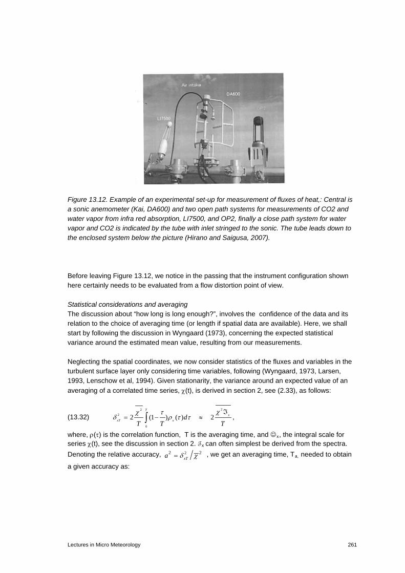
Figure 13.12. Example of an experimental set-up for measurement of fluxes of heat,: Central is a sonic anemometer (Kai, DA600) and two open path systems for measurements of CO2 and water vapor from infra red absorption, LI7500, and OP2, finally a close path system for water vapor and CO2 is indicated by the tube with inlet stringed to the sonic. The tube leads down to the enclosed system below the picture (Hirano and Saigusa, 2007). Before leaving Figure 13.12, we notice in the passing that the instrument configuration shown here certainly needs to be evaluated from a flow distortion point of view. Statistical considerations and averaging The discussion about “how long is long enough?”, involves the confidence of the data and its relation to the choice of averaging time (or length if spatial data are available). Here, we shall start by following the discussion in Wyngaard (1973), concerning the expected statistical variance around the estimated mean value, resulting from our measurements. Neglecting the spatial coordinates, we now consider statistics of the fluxes and variables in the turbulent surface layer only considering time variables, following (Wyngaard, 1973, Larsen, 1993, Lenschow et al, 1994). Given stationarity, the variance around an expected value of an averaging of a correlated time series, χ(t), is derived in section 2, see (2.33), as follows:

(13.32) 22

2

0

2 (1 ) ( ) 2T

xxT x d

T T T

χχ τδ ρ τ τ

ℑ= − ≈∫ ,

where, ρ(τ) is the correlation function, T is the averaging time, and x, the integral scale for series χ(t), see the discussion in section 2. Tx can often simplest be derived from the spectra. Denoting the relative accuracy, 22 2

xTa δ χ= , we get an averaging time, Ta, needed to obtain

a given accuracy as:


(13.33) 2

2

2

2x

xaT

a

χχ

ℑ≈

′

Letting χ = γ, γ’2,w’2, w’γ’, u´w´-- etc. allow one to compute the averaging time, necessary to

obtain a given accuracy for 2, , ,w u wγ γ γ′ ′ ′ ′ ′ etc.. Working with the temperature, θ’, as the

passive scalar Wyngaard (1973) finds the following expressions for necessary averaging times for accuracy a2, assuming that the turbulence variable can be considered a joint Gaussian distributed. (13.34)

,

2 2 , ,2 2 2 2 2, ,

2 2

2 2'2 2 2 2 2

( 1) , 10 , 6 ,( ) ( )( 1) ( 1)

'( ) ( )a auw wa wT K T T

a a a a au w wu w wθθ

θ

θℑ ℑ ℑ ℑ ℑ

≈ − = ≈ = ≈′ ′ ′

− −′ ′ ′

where K is the Kurtosis of the signals θ and w, corresponding to a joint Gaussian process, which is a very good approximation for turbulence signals considered here. Analysis of experimental data was necessary to derive the numerical coefficients in the two last equations, and therefore also applies for “normal” boundary layer turbulence only. Additionally, we can follow Wyngaard (1973) in assuming all the integral timescales to be the same (∼z/U). From (13.34), it is seen that to realize a given accuracy, a, for the eddy correlation fluxes, we need an averaging time 6-10 times longer than what is needed to obtain a variance with the same accuracy, a. In the context of the different flux estimation techniques summarized in this section, it is seen that for the same averaging time, the methods employing power spectra are statistically more accurate than those involving cross-variance, both in raw and spectral forms. Further it is seen that the needed averaging times increases with measuring height, at least within the surface layer. Indeed it quite easily increases to be uncomfortably large. For a = 0.02 and Tx = 1 sec, we obtain: Furthermore, one can study the demands to averaging time for moments of higher order than the variances and co-variances, discussed above. One finds that it becomes almost impossible to determine these higher-order moments in the atmospheric boundary layer with acceptable statistical reliability, because the averaging time must be limited to time periods substantially less than the diurnal cycle to avoid the problems with instationarity. This issue is discussed in section 2, in connection with the discussion of the “spectral gap”, the gap between the fluctuation associated with boundary layer turbulence that can carry the vertical fluxes between the surface and the atmosphere, and the mezzo-scale and synoptic fluctuations. This gap in a sense reflect the largest averaging times, T, one can use for the statistical analysis above, while still maintaining the assumption of a statistically stationary situation. More specific choices can be considered for specific situations where the flow changes more strongly, see e.g. the growth of the unstable boundary layer in the early morning in section 8. This reflects other situations where our mean values changes relatively fast compared to the slowest turbulence time scales, and use of the expressions pertaining to stationary conditions is argued valid by that the conditions can be considered pseudo stationary, meaning exactly that the turbulent scaling from the mean values, developed for stationary

23 4 510 sec; 4 10 sec; 1.2 10 secwT T Tγγ γ′≈ ≈ ⋅ ≈ ⋅


conditions, still apply because the turbulence can change fast enough to follow the changing mean values. Statistical considerations, digital data, aliasing Most data handling are performed digitally today. This raises the problem of the necessary data rate, which can be framed as: “How short is short enough”, referring to the duration between two data scans. We will consider this issue as a question about aliasing. Consider a usual stationary time signal, with its Fourier mode:

(13.35) '( ) ( ) exp( )u t dZ i tω ω∞

−∞= ∫

With associated auto-correlation function and power spectrum:

(13.36)

'( ) ( ) ( ) ( ) exp( )

1( ) ( ) exp( )

2

u t u t R S i d

S R i d

τ τ ω ωτ ω

ω τ ωτ τπ

∞

−∞

∞

−∞

+ = =

= −

∫

∫

We now sample the data with the scanning rate ∆t, to obtain : a(n)=u´(n∆t). -∞<n<∞. From the a´s we can generate that correlation coefficient, as follows: (13.37) '( ) (( ) ) ( ).n n ka a u n t u n k t R k t k+ = ∆ + ∆ = ∆ −∞ < < ∞ ,

Which illustrate that the correlation coefficients derived from the digitized data equals the one for the raw data, u´(t), but only determined for the discreet time intervals. Note also that the variance equal to R(0) is correct. Similarly it is seen that also co-variances is correct. The power spectrum derived from the digitized data can be written:

(13.38) 1

( ) ( ) exp( )2

k

ak

S R k t ik t tω ωπ

=∞

=−∞

= ∆ − ∆ ∆∑ ,

Where subscript a means that the spectrum is generated from the digitized data. We notice that Sa( ω) must be a periodic function with a period of 2π/∆t , since k is an integer. Therefore, we only need to determine Sa(ω) for |ω| < π/∆t, see also Yaglom (1962) . Since the correlation function is the same as for the raw data, we can use (13.36) to write

(13.39) 1

( ) ( ') exp( ( ' )) '2

k

aS S ik t d tω ω ω ω ωπ

=∞ ∞

−∞−∞

= ∆ − ∆∑∫

We now make the k-summation to obtain:

(13.40)

2( ) ( ') ( ' ) ' ,

2 2 2( ) ( ) ( ) ( 2 ) ( )

a

a

S S m d mt

S S S S S mt t t

πω ω δ ω ω ω

π π πω ω ω ω ω

∞

−∞

= − − −∞ < < ∞∆

= + ± + ± + + − − + ± + +∆ ∆ ∆

∫

Where we have used that:

2( ' ) exp( ( ' ))) 2

ktm ik ttπδ ω ω ω ω

π

=∞

−∞

∆− − = ∆ −

∆ ∑

Sa (ω) is seen to be periodic with the period sampling frequency ωs =2π/∆t, and therefore only the spectrum for --π/∆t< ω < π/∆t, contain the information. π/∆t is denoted the Nyquist frequency, ωN. Hence, we see that if S(ω) has energy outside the Nyquist region, |ω| < π/∆t, then Sa(ω) will be deformed by that this energy is folded back into the region of |ω| < π/∆t. This is illustrated on Figure 13.13 while Figure 13.14 reveals how aliasing comes about.

Figure 13.13 The spectral estimates showing the characteristic effect of aliasing. (Lumley and Panofsky (1964), n0 is the Nyquist frequency.

Figure 13.14. The source of aliasing: Sampling a sinusoid at a rate below its frequency. (Lumley and Panofsky (1964) Hence, we are guided to choose a sampling rate that short enough to resolve the spectra undistorted by aliasing. Here we should mention also the possibility of using low pas filters, see section 2, which can reduce the spectrum above the Nyquist frequency, before digitizing, at the prize of reducing the variance. Instationary and inhomogenous conditions One can talk about two different approaches. In the first the measurements are focused on a simple and well defined situation, typical a surface change where the measurement set-up configured to study situations where the wind blow perpendicularly across the line of surface change, see figure 13.5 A and B. This corresponds to the flow situations described in the

beginning of section 9. The situation can obviously not be considered horizontally homogenous, meaning that several masts or measuring points along the x-direction are needed. However, it can mostly be considered stationary and most of the instrument and statistical considerations are similar to the situation for horizontally homogeneous situations, aside from that one has to include considerations about the variation along horizontal directions as well. For example, one will have to include foot prints considerations, i.e. the origin of a surface flux reaching a sensor at a given measurement height, as discussed in section 9 in connection with Figure 9.13.

Figure 13.15 A. Experimental program for inhomogenous flow, with one additional horizontal dimension being important, the one perpendicular on the surface change (water to land, see different modelling possibilities in section 9). - . .


.

Figure 13.15B. A coastal flow experiment, The Risø78.experiment (Højstrup, 1981). Figure 13,16 shows a different type monitoring, where the aim is to conduct the monitoring over a certain area, and use all kinds of different sensors, with all kinds of different resolutions. Here one aims not for specifically simple situation, but more to monitor for an area, and use and compare model output and data interpretations much as possible. However, much of the technical and statistical considerations will be similar to the simpler inhomogeneous situation and the horizontally homogeneous situations, but the flow modifications due to surface change, within each subarea, wind direction, and general ambient conditions, must be evaluated with the model systems described in section 9. See also the discussion in section 12 about wind climate. Spatial resolution and aliasing. However, Figure13.16 also points to the issue of how well the discreet data derived from the many measuring stations do represent the continuous field of meteorological parameters. To analyse this we consider the aliasing discussion for the time series analysis above. Simplifying the discussion to 1 dimension, we can just replace the ω t in (13.35) with k1x, the x-coordinate and the wave number along the x-direction, with ∆x as grid length this direction. Hence, we see that the that the Nyquist wave number as |k1| < π/∆x or the corresponding λ1< ∆x/2. This then give an indication of which scales that should be expected to be influenced by aliasing distortion. Also here one can of course remedy problems by use of filters, and unavoidably do so by the response limitations of the different instruments.

. Figure 13.16. Large scale measuring program spanning a larger area, and employing a wide range of sensors. In the end the data interpretation will be included in a numerical code, where the grids are sketched on to the surface. Also, here one will however, seek to place each ground based sensor to allow an assumption of pseudo stationarity and pseudo horizontal homogeneity.


References

Books: IEC61400-3, 2009, Wind turbines-Part 3: Design of offshore wind turbines. Arpaci, V.S. and P.S. Larsen, 1984: Convection heat transfer Prentice-Hall, 512 pp Arya, S.P. 1988, Introduction to Micrometeorology, Academic Press, San Diego, USA, 307p Arya, S.P. 1999. Air Pollution Meteorology and Dispersion. Oxford University Press, 310p. AutoFlux.1998. An Autonomous System for monitoring Air-Sea fluxes using the Inertial Dissipation Method and Ship Mounted Instrumentation, Final Report EU-Contract MAS3-CT97-0108, Eds.: S.E Larsen and M. Nielsen. www.soc.soton.ac.uk/JRD/MET/AUTOFLUX Chapman, S. and T.G. Cowling, 1970: The mathematical theory of non-uniform gases. Cambridge University Press, Cambridge, 422 pp.

Gumbel, E. J. , 1958: Statistics of Extremes. Columbia University. N.Y., London Holton, J. R., 1992. An introduction to Dynamic Meteorology. Academic Press, Inc, 511p. Kaimal, J.C. and J.J. Finnigan:1994; Atmospheric Boundary Layer Flows, their structure and measurements. Oxford University press, 288p. Ladyzhenskaya, J.A., 1969: The mathematical theory of viscous incompressible flow, Gordon and Breach, Hew York, USA Liss, P.S. and W.G.N. Slinn (eds), 1983: Air-Sea Exchange of Gases and Particles. NATO ASI Series C . No 108. Reidel Publishing Company, 559 p. Lumley, J. L. and H. A. Panofsky (1964). The structure of atmospheric turbulence. Interscience Publishers, J.Wiley& Sons, New York, 239p. Monin, A.S. and A.M. Yaglom, 1971: Statistical Fluid Mechanics: The mechanics of turbulence. MIT Press, Cambridge, Mass.,769p Panofsky, H.A. and J.A. Dutton (1984) Atmospheric Turbulence, Models and Methods for Engineering Applications. John Wiley & Sons, New York, 397 p. Stull, R.B.:1991: An Introduction to Boundary Layer Meteorology. Kluwer. 666 p. Tennekes, H. and J.L. Lumley (1972) A first course in turbulence. MIT, Cambridge, Mass. 300p. Troen, I. And Petersen, E L. , 1989, European Wind Atlas. Risø, Roskilde, Denmark. 656 p. Wallace, JM, PV Hobbs (2006) Atmospheric Sciences, 2nd ed. Academic Press, 467 p. Yaglom, A.M.: 1962. An introduction to the theory of Stationary Random Functions. Prentice-Hall, Inc. 234p Zilitinkevich, S.S., 1991: Turbulent penetrative convection. Avebury Technical, Aldershot, U.K., 179 p. Journals and reports Abild, J. B,, N.G. Mortensen and L. Landberg, 1992. Application of the wind-atlas method to extreme wind speed data. Proceedings of the 8th International Conference on Wind Engineering, Canada 1991, J. Wind Eng. and Ind. Aerodyn., 41, 473-484. Andreas, E.L., 1980: Estimation of heat and mass fluxes over arctic leads. Mon. Wea. Rev., 108, 2057-2063. Arya, S.P.S., 1973: Contribution of form drag on pressure ridges to the air stress on arctic ice. J. Geophys. Res., 78, 7092-7099.


http://www.soc.soton.ac.uk/JRD/MET/AUTOFLUX

Araya, S.P.S., 1978: Comparative effects of stability, baroclinity and the scale-height ratio on drag laws for the atmospheric boundary layer. J. Atmos. Sci., 35, 40-46. Batchelor, G.K. and I. Proudmann, (1954) The effect of rapid distortion on a fluid in turbulent motion. Quart. J. Mech. Appl. Math., 7, 83-103. Belcher, S.E., D.P. Xu, and J.C.R.Hunt, 1990: The response of a turbulent boundary layer to arbitrarily distributed two-dimensional roughness changes. Quart. J. Roy. Met. Soc., 116, 611-635. Berkowicz, R. and L.P. Prahm, 1979: Generalization of K-theory for turbulent diffu-sion. Part 1: Spectral turbulent diffusivity concept. J. Appl. Meteor., 18, 266-272. Brandt, J. 1998: Modelling Transport, Dispersion and Deposition of Passive Tracers from Accidental Releases. PhD thesis, Risø National Laboratory & National Environmental Research Institute, Risø/ NERI. Britter, R.E., J.C.R. Hunt, K.J. Richards (1981) Air-flow over a two dimensional hill: studies of velocity speed up, roughness effects and turbulence. Quart. J. R. Met. Soc., 107, 91-110. Brown, R.A., 1980: Longitudinal instabilities and secondary flows in the planetary boundary layer: a review. Rev. Geophys. Space Phys., 18, 683-697. Brutsaert, W., 1975: Comments on surface roughness parameters and the height of dense vegetation. J. Met.Soc. Japan, 53, 96-97. Brutsaert, W.H., 1982: Exchange processes at the earth atmosphere interface. In: Engineering Meteorology, Ed. E. Platte, Elsevier, 319-369. Busch, N.E., 1973: On the mechanics of atmospheric turbulence. In: Workshop on Micrometeorology. Ed.D.A. Haugen, American. Meterological Society, Boston, Mass., USA, 1--28. Busch, N.E., 1975: Fluxes in the surface boundary layer over the sea. In: Modelling and prediction of the upper layers of the ocean. NATO ASI, Ed. E.B.Kraus, 72-91. Busch, N.E., S.E. Larsen and D.W. Thomson, 1979: Data analysis of atmospheric measurements. Proceedings of the Dynamic Flow Conference 1978. Eds. E.G.K. Kovasznay et al., Dantec, Skovlunde, Denmark, 887-908. Busch, N.E., O.Christensen, L.kristensen.L.Lading and S.E.Larsen, 1980: Cups, Vanes, propellers and Laser anemometers. In: Air-Sea Interaction. Ed’s. F.Dobson, L.Hasse and R.Davis. Plenum Press. 11-46. Businger, J.A., J.C. Wyngaard, Y. Izumi, and E.F. Bradley, 1971: Flux-profile relationships at the atmospheric surface layer. J. Amos. Sci., 28, 191-189. Businger, J.A. and S.P.S. Arya, 1974: Height of the mixed layer in the stably stratified planetary boundary layer. J. Atmos. Sci., 18, 181-189. Businger, J.A., 1982: Equations and concepts. In: Atmospheric Turbulence and Air Pollution Modelling, Eds.F.T.M. Nieuwstadt and H. van Dop, Reidel, Dordrecht, Holland, 1-36. Caughey, S.J., 1982: Observed characteristics of the atmospheric boundary layer. In: Atmospheric Turbulence and Air Pollution Modelling, Eds. F.T.M. Nieuwstadt and H. van Dop, Reidel, Holland, 107-158. Charnock, H., 1959: Wind stress on a water surface. Quart. J. Roy. Met. Soc., 81, 639-640. Clarke, R.H. and G.D. Hess, 1973: On the appropriate scaling for velocity and temperature in the planetary boundary layer. J. Atmos. Sci., 30, 1346-1353. Claussen, M., 1991: Local advection processes in the surface layer of the marginal ice zone boundary layer. Boundary-Layer Meteorol., 30, 327-341.


Courtney, M. and I. Troen, 1990: Wind speed spectrum from one year of continuous 8 Hz measurements. Proceedings of Ninth Symposium on Turbulence and Diffusion, American Meteorology Society, Boston, USA, 301--304. Cristen, A, (2004) Micro scale Weather and Climate. Course. Dept Geography, Univ. British Columbia. Davenport, A G. (1961). The application of statistical concepts to the wind loading of structures. Proc. Inst. Civ. Eng. (London) 19,449-472. Deardorff, J.W., 1970: Convective velocity and temperature scales for the unstable planetary boundary layer and for Rayleigh convection. J. Atmos. Sci., 27, 1211-1213. Deardorff, J.W., 1972: Parameterization of the planetary boundary layer for use in general circulation models. Mon. Wea. Rev., 100, 93-100. Deardorff, J.W., 1972: Numerical investigation of neutral and unstable planetary boundary layers. J. Atmos. Sci. 29, 91-115. Delage, Y., 1988: A parameterization of the stable atmospheric boundary layer. Boundary-Layer Meteorol., 43, 365-381. Dunkerley, F N, T Mikkelsen, S E Larsen, P Astrup, 2003: Comparison of a simel model for the coastal boundary layer with data from the Schiermonkoog experiment, Geophys. Abstract, vol 5. 2003. Dyer, A.J., 1974: A review of flux-profile relationships. Boundary-Layer Meteorol., 7, 363-372. Dyer, A.J., 1981: Flow distortion by supporting structures.Boundary-Layer Meteorol., 20, 243-251. Dyer, A.J., 1982: Reply (to comment by J.C. Wyngaard).Boundary-Layer Meteorol., 22, 267-268. Edson, J.B., C.W. fairall, P.G. Mastayer and S.E. Larsen (1991) A study of the inertial dissipation method for computing air-sea fluxes. J. Geophys. Res. 96 C610689-10711. Ekman, V.W., 1905: On the influence of the earth rotation on ocean curents. Arkiv, Math. Astron. O. Fysik, 2, 11. Emeis, S, HP Frank, F Fiedler, 1995: Modification of air-flow over an escarpment-results from the Hjardemål experiment. Boundary Layer Meteorol. 74, 161-160. Elliott, J.A., 1972: Microscale pressure fluctuations measured within the lower atmospheric boundary layer. J. Fluid Mech., 53, 351-383. Esau, I., 2004: Simulation of Ekman boundary layers by large eddy model with dynamic mixed subfilter closure. J. Env. Fluid Mech., 4(2), 203-303. Esau,I., N. and S. Zilitinkevich, 2006. Universal Dependence between Turbulent and Mean Flow Parameters in Stably and Neutrally Stratified Planetary Boundary Layers, Estournel, C. and D. Guedalia, 1987: A new parameterization of eddy diffusivities for nocturnal boundary layer modelling. Boundary-Layer Meteorol., 39, 191-302. Fairall, C. W. And S. E. Larsen, 1984: Dry depositionsurface production and dynamics of aerosols in the dynamic boundary layer. Atmos. Env., 18, 69-77. Fairall, C.W., 1987: A top-down and bottom-up diffusion model of CT

2 and Cq2 in the entraining

convective boundary layer. J. Atmos. Sci., 6, 1010-1017. Frandsen, S.: 1992: On the wind speed reduction in the center of a large cluster of wind turbines. Jourm. Of Wind Engineering and Industrial Aerodynamics, 39, 251-265. Frandsen, S.T. (2007) Turbulence and turbulence generated structural loading in wind turbine clusters. Risø-R- 1188(EN 130p Frank, H. P. (1996) A simple spectral model for the modification of turbulence in flow over gentle hills. Boundary-Layer Meteorology, 79, 345-373.


Frank, H. P., S. E. Larsen, J. Højstrup (2000) Simulated wind power off-shore using different parameterizations for the sea surface roughness. Wind Energy, 3, 67-79. Friehe, CA, JA Smith, KF Rieder, NE Huang, J-P Giovangeli, GL Geernaert (2001) Win stress and wave direction, 232-241. Chapter 12 in: Jone, S F and Y. Toba, eds. (2001) Wind Stress over the Ocean. Cambridge University Press, 307 p. Garratt, J.R., 1978: Flux profile relations above tall vegetation. Quart. J. Roy. Met. Soc., 104, 199-211. Geernaert, G. L. (1990) Bulk Parameterizations for the wind stress and the heat flux. In Surface waves and fluxes: Theory and remote sensing. Vol.1. G. Geernaert and W. Plant, eds. 91-172. Gryning S E., L. Mahrt, S E Larsen (1985) Oscillating nocturnal slope wind in a coastal valley. Tellus, 374, 196-203. Gryning, S-E., A.P. vanUlden and S. E. Larsen 1983. Dispersion from a continuous ground level source investigated by a K-model. Quart.J.R.Meteorol. Soc. 109, 355-364. Gryning, S.E., 2006: The height of the atmospheric boundary layer during unstable conditions. Risø-R-1536. 63 p. Gryning, S.E. and E. Batchvarova,1990: Analytical model for the growth of the coastal internal boundary layer during onshore flow. Quart. J. Roy. Met. Soc., 116, 187-203. Gryning, S.-E.; Batchvarova, E.; Brümmer, B.; Jørgensen, H.E.; Larsen, S.E., 2007, On the extension of the wind profile over homogeneous terrain beyond the surface boundary layer. Boundary-Layer Meteorol. 124: 251-268. Hansen, C. and S.E. Larsen (1997) Further work on the Kitaigorodskii roughness length model. A new derivation using Lettau’s expression on steep waves. Geophysica, 33 no 2, 29-44. Hasager, C.B. and N.O. Jensen, 1999: Surface-flux aggregation in heterogeneous terrain. Quart. J. Roy. Met. Soc., 125, 2075-2102. Hasager, C.B.; Nielsen, N.,W.; Jensen, N.O.; Bøgh, E.; Christensen, J.H.; Dellwik, E.; Søgaard, G.. (2003), Effective roughness calculated from satellite-derived land cover maps and hedge-information used in a weather forecasting model. Boundary-Layer Meteorol. v. 109 p. 227-254 Hasse, L., 1976: A resistance-law hypothesis for the nonstationary advective planetary boundary layer. Boundary-Layer Meteorol., 10, 393-07. Hill, R.J., 1989: Implications of Mounin-Obukhov similarity theory for scalar quantities. J. Atmos. Sci., 46, 2236-2244. Hirano, T. And N. Saigusa, 2007: Practise of Flux Observations in Terrestrial Ecosystems. Chapter 3: Flux Measurement using the eddy co-variance method. AsiaFlux Steering Committee (ed.) 3-1, 3-21: www.asiafluxnet/members/material/ Holtslag, A.A.M. and F.T.M. Nieuwstadt, 1986: Scaling in the atmospheric boundary layer. Boundary-Layer Meteorol., 36, 201-209. Horst, T.W. and J.C. Weil, 1991: Footprint estimation for scalar flux measurements in the atmospheric surface layer. Boundary-Layer Meteorology, 59, 279-296. Hunt, J.R.C. and D.J. Carruthers,1990:Rapid distortion theory and the problems of turbulence. J.Fluid Mech. 212, 497-532 Hunt, J.C.R. and J.E.Simpson, 1982: Atmospheric Boundary Layers over Non-Homogeneous terrain. In: Engineering meteorology (E.: E. Plate) Elsevier, Amsterdam. 269-318. Hunt, J C R, W H Snyder, R E Lawson Jr., 1978; Flow structure and turbulent diffusion around a three dimensional hill. In Fluid Modelling study on effects of stratification. Part I Flow structure, Report EPA-600/4-78-041, US-Environmental Protection Agency, 1978.


Högström, U., 1990: Analysis of turbulence structure in the surface layer with a modified similarity formulation for near neutral conditions. J. Atmos. Sci., 47, 1949-1972. Højstrup, J., 1981: A simple model for adjustment of velocity spectra in unstable conditions downstream an abrupt change in surface roughness and heat flux. Boundary-Layer Meteorol., 21, 341-356. Højstrup, J., 1982: Velocity spectra in the unstable planetary boundary layer. J. Atmos. Sci., 39, 2239-2248. Højstrup, J., S.E. Larsen, and N.O. Jensen, 1982: Results from an experimental investigation of a step change in surface heat flux. Proceedings of First International Conference on Meteorology and Air-Sea Interaction of the Coastal Zone. American Meteorology Society, Boston, USA, 28-30. Højstrup, J., S.E. Larsen, and P.H. Madsen, 1990: Power spectra of horizontal wind components in the neutral atmospheric surface boundary layer. Proceedings of Ninth Symposium on Turbulence and Diffusion. American Meteorological Society, Boston, USA, 305--308. Ibrom, A., E. Dellwik, S. E. Larsen, K. Pilegaard, 2007: On the use of the Webb-Pearman-Leuning theory for closed-path eddy correlation measurements. Tellus, 1-10. Izumi, Y, 1971: The Kansas 1968 Field Program Data Report. Environmental Research Papers No. 379, AFCRL-72-0041. Air Force Cambridge Research Laboratories, Bedford, Mass. US. Izumi, Y, and SJ Changhey, 1976: Minnesota 1973 Atmospheric Boundary Laye Experiment Data Report. AFCRL Research Papers No. 547, AFCRL-TR-76-0038. Cambridge Research Laboratories, Bedford, Mass. US. Jackson, P.S. and J.R.C. Hunt, 1975: Turbulent wind flow over a low hill. J. Roy. Met. Soc., 101, 929--955. Jackson, P.S., 1981: On the displacement height in the logarithmic velocity profile. J. Fluid Mech., 111, 15-25. Jensen, N. O and E. W. Peterson, 1977. Wind flow near the surface over non-uniform terrain. Progress report for 1976 for US Army Grant) Jensen, N. O., 1978: Change of surface roughness and the planetary boundary layer. Quart. J.R. Meteorol. Soc. , 104, 351-356. Jensen,N.O. and N. E. Busch, 1982: Atmospheric Turbulence. In: Engineering meteorology (E.: E. Plate) Elsevier, Amsterdam.179-231. Jensen, N.O. (1983) Escarpment induced flow perturbations, a comparison of measurements and theory. Journ. Wind Engirneering and Industrial Aerodynamics. 15, 243-251. Jensen, N.O., Petersen, E.L. and Troen, I. (1984) Extrapolation of Mean Wind statistics with Special Regard to Wind Energy Applications. WMO. World Climate Programme Report No. WCP-86, 85 pp. Jensen, N.O., 1991: Comments on surface parameterization. Proceedings of WMO Planetary Boundary Layer Model Evaluation Workshop, August, 1989, Reading UK. Ed. J.C. Wyngaard, WMO/TD-No. 378, 40--42. Jone, ISF, Y Volkov, Y Toba, S Larsen, NE Huang (20011) Overview of Wind Stress over the Ocean,1-33. Chapter I in Jone, ISF and Y. Toba, eds. (2001) Wind Stress over the Ocean. Cambridge University Press, 307 p. Kaimal,J.C., J.C.Wyngaard and D.A. Haugen, 1968: Deriving power spectra from a three-component sonic anemometer. J. Appl. Meteor., 7, 827 – 837. Kaimal, J.C., J.C. Wyngaard, Y. Izumi, and O.R. Coté, 1972: Spectral characteristics of surface-layer turbulence. Quart. J. Roy. Met. Soc., 563--589.


Kaimal, J.C., J.C. Wyngaard, D.A. Haugen, O.R. Coté, S.J. Caughey, and C.J. Readings, 1976: Turbulence structure in the convective boundary layer. J. Atmos. Sci., 33, 2152--2169. Kristensen, L and NO Jensen (1979) Lateral coherence in isotropic turbulence and with the natural wind. Bound- Lay Meteorol., 17, 353-373. Kristensen, L., HA Panofsky, SD Smith (1981) Lateral coherence of longitudinal wind components in strong winds. Bound-Layer Meteorol.21, 199-205. Kristensen L., 1989: In search of a gust definition. Risø report-M-2796, 22p Kristensen, L., J. Mann, S.P.Oncley, J.C. Wyngaard, 1997: How close is close enought, when measuring scalar fluxes with displace sensors?, Journ Atmos. And Ocean. Technology, 14, 814821. Kristensen, L., DH Lenschow, D Gurarie, and N O Jensen, 2010: A simple model for the vertical transport of reactive species in the convective atmospheric boundary layer. Bound.-Layer Meteorol. 195-221. Lange, B., S.E.Larsen, J. Højstrup and R. Barthelmie, 2004: The influence of thermal effects on the wind speed profile of the coastal marine boundary layer. Boundary-Lay. Meteorol., 112, 587-617 Larsen, S.E., J.Høstrup and C.H.Gibson, 1980: Fast response temperature sensors. In: Air-Sea Interaction. Ed’s. F.Dobson, L.Hasse and R.Davis. Plenum Press. 269-292. Larsen, S.E, K. Hedegaard, and I. Troen, 1982: Change of terrain roughness problem extended to mesoscale fetches. First International Conference on Meteorology and Air/Sea Interaction. American Meteorological Society, Boston, USA, 8-13. Larsen, S.E. and J. Højstrup, 1982: Spatial and temporal resolution of a thin wire resistance thermometer. J. Phys. E: Sci. Instrum., 15, 471-477 Larsen, S.E., N.O. Jensen, 1983: Summary and Interpretation of Some Danish Climate Statistics; Risø-R-399, 76 p. Larsen, S.E., H.R. Olesen, and J. Højstrup, 1985:Parameterization of the low frequency part of spectra of horizontal velocity components in the stable surface boundary layer. In: Turbulence and Diffusion in Stable Environments. Ed. J.C.R. Hunt, Clarendon, Oxford, UK, 181-204. Larsen, S.E., M. Courtney, L. Mahrt, 1990: Low frequency behaviour of horizontal velocity spectra in stable surface layers. Proceedings of Ninth Symposium on Turbulence and Diffusion, American Meteorological Society, Boston, USA, 401-404. Larsen, S.E. , 1993: Observing and modelling the planetary boundary layer. In: Energy and water cycles in the climate system. Ed.s E. Raschke and D. Jacob. NATO ASI seriesI vol5. Springer Heidelberg Germany, 365-418. Larsen, S.E., H.E. Jørgensen, L.Landberg and J.E. Tillman, 2002: Aspects of the atmospheric surface layer on Mars and Earth. Bound. Layer Meteorol.,105, 451-470. Larsen, S.E., J.B.Edson, C.W. Fairall and P.G. Mestayer, 1993: Measurement of temperature spectra by a sonic anemometer. J. Atmos. and Ocean Technology, 10 no 3, 345- 354. Larsén, X. G., C. Vincent and S.E. Larsen ,2013. Spectral structure of the mesoscale winds over the water. Quart. J. Roy. Met. Soc.,139, 685-700. Lenschow, D. H. and A. C. Delany, 1987: An analytic formulation for NO and NO2 flux profiles in the atmospheric surface layer. J. Atmos. Chem., 5, 301-309. Lenschow, D. H., J. Mann, L. Kristensen (1994) How long is long enough when measuring fluxes and other turbulence statistics? J. Atmos. Ocean Techn.,11, 1994, 661-672 Lettau, H., 1969: Note on aerodynamic roughness-parameter estimation on the basis of roughness-element distribution. J. Appl. Met., 8, 828-832.


Lilly, D K (1966) On the application of the eddy viscoscity concept in the inertial subrange of turbulence. NCAR Tech. Rep. 123, National Center for Atmospheric Research, 18pp Mahrt, L., 1985: The vertical structure and turbulence in the very stable boundary layer. J. Atmos. Sci., 42, 2333-2349. Mahrt, L. and S. Larsen, 1982: Small scale drainage front. Tellus, 34, 579-587. Mahrt, L., 1986: On the shallow motion approximations. J. Atmos. Sci., 43, 1036--1044. Mahrt, L. and S. Larsen, 1990: Relation of slope winds to ambient flow over gentle terrain. Boundary-Layer Meteorol.,53, 93--102. Mahrt, L. 1996: The bulk aerodynamic formulation over heteorogeneous surfaces. Bound. Layer Meteorol.,78, 77-119. Makin, V. K. (2005) A note on the drag of the sea surface at hurricane winds. Boundary Layer Meteorology, 115, 169-175. Mann, J. 1994, The spatial structure of neutral atmospheric surface layer turbulence. J. Fluid Mech., 273, 141-168. Mann, J. , 1998. Wind field simulation, Prob. Engng. Mech. Volume 14, no 4, 269-282, Mason, P.J., 1988: The formation of area-averaged roughness lengths. Quart. J. Roy. Met. Soc., 114, 399--420. McBean, G.A. and J.A. Elliott, 1975: The vertical transport of kinetic energy by turbulence and pressure in the boundary layer. J. Atmos. Sci., 32, 753--766. Melgarejo, J.W. and J.W. Deardorff, 1974: Stability functions for the Boundary layer resistance laws based on observed boundary layer heights. J. Atmos. Sci., 31, 1324--1333. Melas, D., 1998, The depth of the stably stratified internal boundary layer over the sea. Geophysical Research Letters, 25, No 13, 2261-2264. Mortensen, N. G. and E.L. Petersen (1997). “Influence of topographical input data on the accuracy of wind flow modelling in complex terrain”. 1997 European Wind Energy Conference, Dublin, Ireland. Mikkelsen, T., Larsen, S.E. and Thykier-Nielsen, S. (1984). Description of the Risø puff diffusion model. Nuclear Tech., 67, 56-65. Mikkelsen, T., Larsen, S.E. and Pecseli, H.L. (1987). Diffusion of Gaussian Puffs. Quart. J.R. Met. Soc., 113 No. 475, 81-105. Mizuno, T. and H.A. Panofsky, 1974: The validity of Taylor's hypothesis in the atmospheric boundary layer. Boundary-Layer Meteorol., 9, 375 --382. Mortensen, N.G., S.E. Larsen, I. Troen, and T. Mikkelsen, 1987: Two years worth of turbulence data recorded by a sonic-anemometer-based data aquisition system. Sixth Symposium on Meteorology and Instrumentation. American Meteorological Society, Boston, USA, 393-396. Mortensen, N.G., L. Landberg, I. Troen E.L. Petersen, 1992: Wind atlas analysis and application program (\wasp).User's Guide. ISBN 87-550-1789-4. Ris› National Laboratory, Roskilde, Denmark, 130 pp. Newley, T.M.J., 1985: Turbulent air flow over hill. Dissertation, University, University of Cambridge, Cambridge, UK, Nicholls, S. and G.J. Readings, 1979: aircraft observations of the structure of the lower boundary layer over the sea. Quart. J. Roy. Met.Soc., 105, 785--802. Nieuwstadt, F.T.M., 1984: The structure of the stable nocturnal boundary layer, J. Atmos. Sci., 41, 2202--2216. Nielsen, M. And SE Larsen (2002)The influence of pulse firing delays on sonic anemometer responce characteristics. Proc. 151h AMS Symposium on boundary layers and turbulence.


Wageningen, The Netherlands,15-19 July (American Meteorological Society, Boston, Maa, US) 139-142. Obukhov, A.M., 1971: Turbulence in an atmosphere with non-uniform temperature. Boundary-Layer Meteorol., 2, 7--29. Olesen, H.R., S.E. Larsen, and J. Højstrup, 1984: Modelling velocity spectra in the lower part of the planetary boundary layer. Boundary-Layer Meteorol., 29, 285--312. Oncley, S.P., J.A. Businger, C.A. Friehe, J.C. LaRue, E.C.Tsweire, and S.S. Chang, 1990: Surface layer profiles and turbulence measurements over uniform land under neutral conditions. Proceedings of Ninth Symposium on Turbulence and Diffusion. American Meteorological Society, Boston, USA, 235--240. Panofsky, H A ; 1978. Matching in the convective planetary boundary layer. J. Atmos. Sci., 15, 272-276. Panofsky, H.A., D. Larko, R.C. Lipschutz, G. Stone, F.F. Bradley, A.J. Bowen, and J. Højstrup, 1982. Spectra of velocity components over complex terrain.Quart. J. Roy. Met. Soc., 108, 215--230. Peña, A., S.-E. Gryning and C. B. Hasager (2008) Measurements and Modelling of the Wind Speed Profile in the Marine Atmospheric Boundary Layer,. Boundary Layer Meteorol. 129, 479-495. Pena, A., T. Mikkelsen, S.E. Gryning, C.B. Hasager, A.N. Hahmann, M. Badger, I. Karagali and M. Coutney, Offshore vertical wind shear. Final report NORSEWIND work task 3,1, DTU Wind Energy reort 0005 (EN), 2012 Peña, A., C. B. Hasager, J. Lange, J. Anger, M. Badger, F. Bingöl, O. Bischoff, J-P. Caribou, F. Dunne, S. Emeis, M. Harris, M. HofsässI. Karagali, J. Laks, S.E. Larsen, J. Mann, T. Mikkelsen, K.Y. Pao, M. Pitter, A. Rettenmeier, A. Sathe, F. Scanzani, D. Schilipf, E. Simley, C. Slinger, R. Wagner, I. Würth. 2013. Remote Sensing for Wind Energy. DTU Wind Energy E-Report-0029 (EN) 309p, Pollard, R.T., P.B. Rhines, and R.O.R.Y. Thomson, 1973: The deepening of the wind mixed layer. Geophys. Fluid Dyn., 4, 297-304. Powell, D.C. and C.E. Elderkin, 1974: An investigation of the application of Taylor's hypothesis to the atmospheric boundary layer turbulence. J. Atmos. Sci., 31, 990-1002. Rao, K.S., J.C. Wyngaard and O.R. Coté, 1974: The structure of two-dimensional internal boundary layers over a sudden change of surface roughness. J. Atmos. Sci., 31, 738-746. Rao, K.S., J.C. Wyngaard and O.R.Coté, 1974a: Local advection of momentum, heat, and moisture in micrometeorology. Boundary-Layer Meteorol.,7, 331-348. Raupach, M.R., 1979: Anomalies in flux-gradient relationships over forest. Boundary-Layer Meteorol.,16, 467-486. Rice, S.O., 1944,1945, Mathematical Analysis of Random Noise, Bell. Syst. Tech. J. 23, 282-332, 24, 46-156. Savelyev, S. A. and P. A. Taylor, 2005: Internal Boundary Layers: I. Height formulae for neutral and diabatic flows. Boundary-Layer Meteorol.,115, 1-25. Sempreviva, A.M., S.E. Larsen, N.G. Mortensen, and I. Troen, 1989: Response of neutral boundary layers to changes of roughness. Boundary-Layer Meteorol., 50, 205-225. Shodor, Shodor Educational Foundation,Metgroup, Atmospheric Energy balance. On-line course(1996) Smedman, A.S., H. Bergström and B. Grisoggono , 1997: Evolution of stable internal boundary layers over a cold sea. Journ. Geophys. Research, 102, No C1, 1091-1099. Sorbjan, Z., 1986: Local similarity of spectral and cospectral characteristics in the stable continuous boundary layer. Boundary-Layer Meteorol., 35, 257-275.


Stull, R.B., 1988: An introduction to boundary layer meteorology. Kluwer, 666 pp. Taylor, P.A., 1987: Comments and further analysis on the effective roughness length for use in numerical three-dimensional models. Boundary-Layer Meteorol., 39, 402--419. Taylor, P. K. and M.J. Yelland , 2001. The dependence of the sea surface roughness height on the height and the steepness of the waves. Journ. Phys. Oceanography, 31, 572-590. Tennekes, H., 1973: The logarithmic wind profile. J.Atmos. Sci., 30, 234--238. Tennekes, H. and A.G.M. Driedonks, 1981: Basic entrainmentequations for the atmospheric boundary layer. Boundary-Layer Meteorol., 20, 515--531. Tennekes, H., 1982: Similarity relations, scaling laws and spectral dynamics. In: Atmospheric Turbulence and AirPollution Modelling. Eds. F.T.M. Nieuwstadt and H. van Dop,Reidel Publications, Dordrecht, Holland, 37-68. Thom, A.S., 1971: Momentum absorption by vegetation. Quart. J. Roy. Met. Soc., 97, 414-428. Tillman, J.E., L.Landberg, and S.E.Larsen, 1994: The boundary layer of Mars: Fluxes, stability, turbulent spectra, and the growth of the mixed layer. J. Atmos. Sci., 51, 1709-1727. Troen, I., N. O. Jensen, L. Kristensen, S. E. Larsen, 1990: A high resolution spectral model for flow in complex terrain. Proc. Symposium on turbulence and diffusion Risø. American Meteorological Society, Boston. 417-420. Troen, I., T. Mikkelsen, and S.E.Larsen, 1980: Note on spectral diffusivity theory. J. Appl. Meteor.,19,609-615. Troen, I. and E.L. Petersen, 1989: European Wind Atlas. Risø National Laboratory, Roskilde. Denmark. Townsend, A.A. , 1976, The structure of turbulent shear flow, 2nd ed. Cambridge uni. Press 429pp Ulden, A.P. van, and A.A.M. Holtslag, 1980: The wind at heights between 10m and 200m in comparison with the geostrophic wind. Seminar on radioactive releases and their dispersion in the atmosphere following a hypothetical reactor accident, Vol 1. Published by E.C. Commission,Luxemburg. WAsP Engineering, Course Notes, 2008: Wind Energy Department, Risø National Laboratory, version 2. Walmsley, J.L., I. Troen, D.P. Lalas, and P.J. Mason, 1990:Surface layer flow in complex terrain: Comparison of models and full-scale observations. Boundary-Layer Meteorol., 52, 259-289. Wieringa, J. 1976: An objective exposure correction method for average wind speeds measured at a sheltered location. Quart. J. Roy. Met. Soc., 102, 867--889. Wood, N. and P. Mason, 1991: The influence of static stability on the effective roughness length for momentum and heat transfer. Quart. J. Roy. Met. Soc., 117, 1025--1056. Wyngaard, J.C. and O.R. Coté, 1971: Cospectral similarity in the atmospheric surface layer. Quart. J. Roy. Met. Soc., 98, 590--603. Wyngaard, J.C. and O.R. Coté, 1972: The budgets of turbulent kinetic energy and temperature variance in the atmospheric surface layer. J. Atmos. Sci., 28, 190--201. Wyngaard, J.C. 1973: On surface-layer turbulence. Proceedings of Workshop on Micrometeorology. Ed. D.A.Haugen,American Meteorological Society, Boston, USA, 102--149. Wyngaard, J.C., S.P.S. Arya and O.R. Coté,1974: Some aspects of the structure of convective planetary boundary layers. J. Atmos. Sci., 31 no. 3, 747-754. Wyngaard, J.C. and S.F. Clifford, 1977: Taylor's hypothesis and the high-frequency turbulence spectra. J. Atmos. Sci., 34, 922--929.


Wyngaard, J.C. 1982: Boundary-layer modelling. In:Atmospheric Turbulence and Air Pollution Modelling, Eds.F.T.M. Nieuwstadt and H. van Dop, Reidel publications, Dordrecht, Holland, 69-106. Wyngaard, J.C.and R.A. Brost, 1984: Top-down and bottom-up diffusion of a scalar in the convective boundary layer. J. Atmos. Sci., 41, 102-112. Wyngaard, J.C., 1982a: Atmospheric turbulence measurements. J. Appl. Meteor., 20, 784-794. Wyngaard, J.C., 1982b: Comments on `Flow distortion by supporting structures' by A.C. Dyer. Boundary-Layer Meteorol., 22,263--265. Wyngaard, J.C., 1988: The effects of probe induced flow distortion on atmospheric turbulence measurements: extension to scalars. J. Atmos.Sci., 45, 3400-3412. Zeman, O. and N.O. Jensen, 1987: Modification of turbulence characteristics in flow over hills. Quart. J. Roy. Met. Soc., 113, 55--80. Zilitinkevich, S.S., 1972: On the determination of the height of the Ekman boundary layer. Boundary-Layer Meteorol., 3, 141--145. Zilitinkevich, S.S., 1975: Resistance laws and prediction equations for the depth of the planetary boundary layer. J. Atmos. Sci., 32, 741--752. Zilitinkevich, S., I Mamarella, A. Baklanov, 2009: The effect of stratification on the aerodynamic roughness length. In Meteorological and Air Quality Models for Urban Areas. DOI 10.1007/978-3-642-00298-4_7, Springer, 2009, 59-66.


Acknowledgements

These lecture notes have been put together in a span of about 20 years. I wish to thank all my colleagues, with whom I have discussed the various subjects over the years. Similarly, I wish to thank all the students, at the “Micro Sale Meteorology” course at the Geophysics Department of Copenhagen University, 1993-2012. Their questions have forced me to look into new issues and new methods within the various subjects, and thereby expanded my knowledge as well this collection of notes.


lectures in micro meteorology - dtu...

Documents