lecture i a gentle introduction to markov chain monte carlo (mcmc)
TRANSCRIPT
Lecture I
A Gentle Introduction to
Markov Chain Monte Carlo (MCMC)
Ed GeorgeUniversity of Pennsylvania
Seminaire de PrintempsVillars-sur-Ollon, Switzerland
March 2005
1
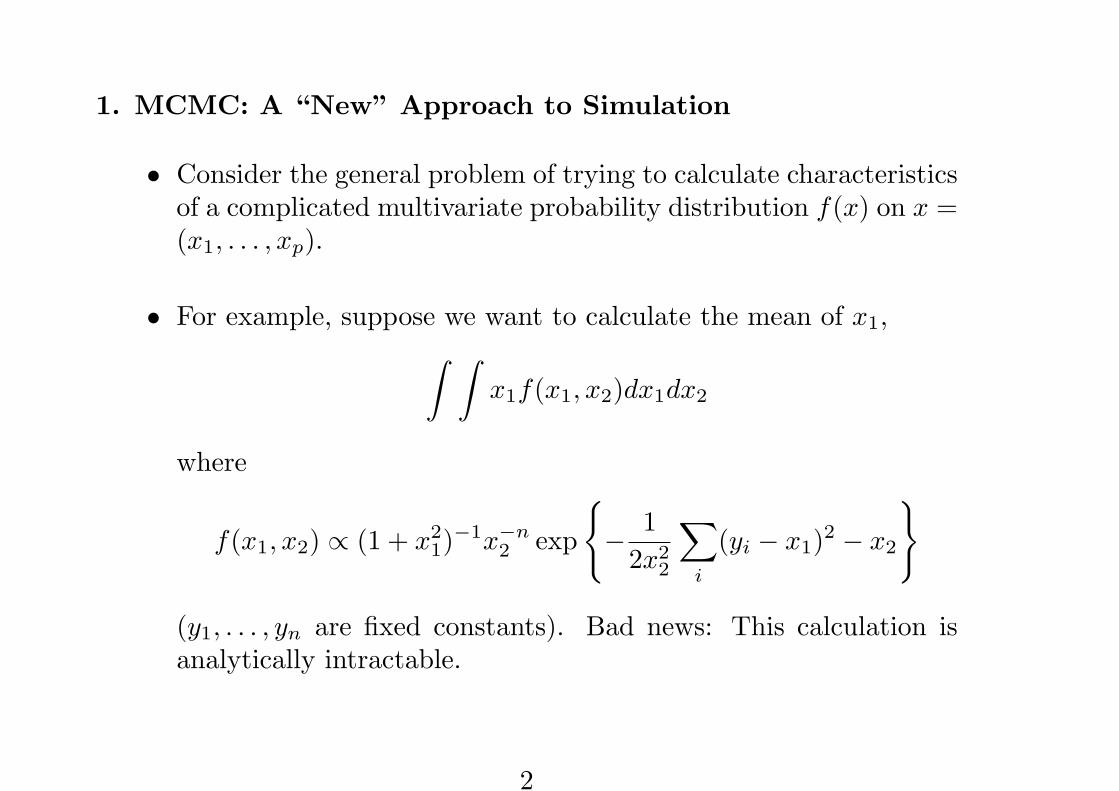
1. MCMC: A “New” Approach to Simulation
• Consider the general problem of trying to calculate characteristicsof a complicated multivariate probability distribution f(x) on x =(x1, . . . , xp).
• For example, suppose we want to calculate the mean of x1,∫ ∫
x1f(x1, x2)dx1dx2
where
f(x1, x2) ∝ (1 + x21)−1x−n
2 exp
{− 1
2x22
∑
i
(yi − x1)2 − x2
}
(y1, . . . , yn are fixed constants). Bad news: This calculation isanalytically intractable.
2
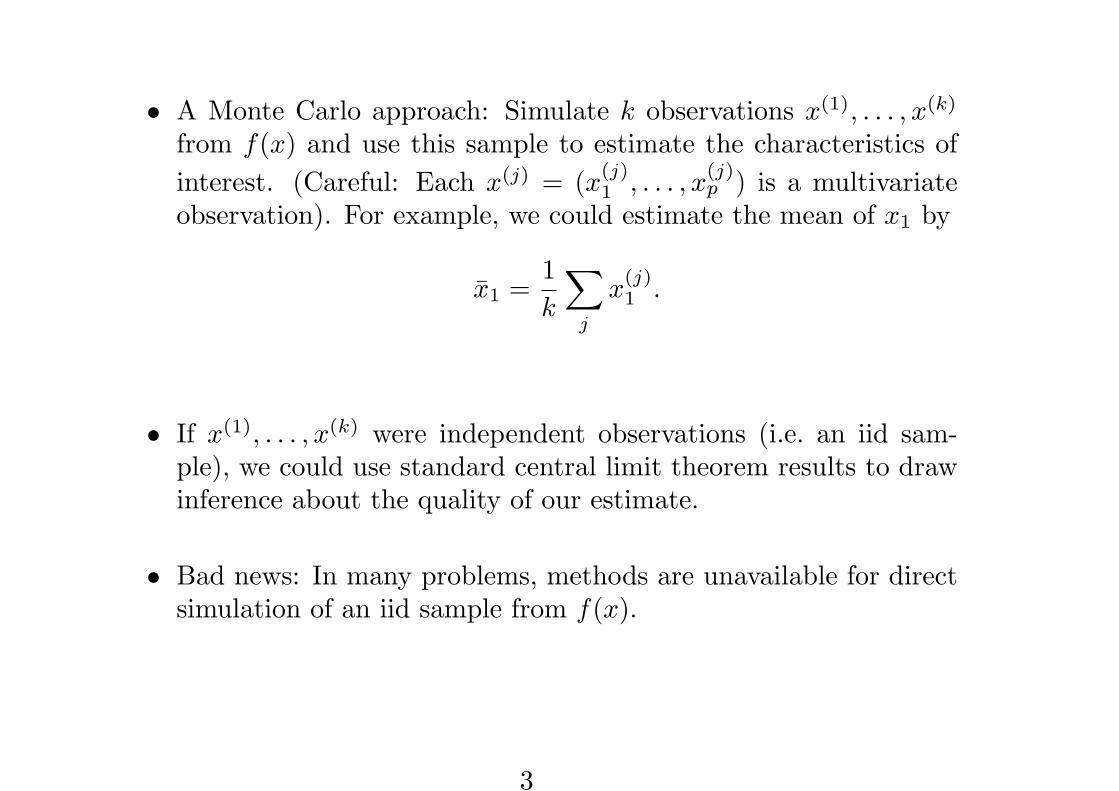
• A Monte Carlo approach: Simulate k observations x(1), . . . , x(k)
from f(x) and use this sample to estimate the characteristics ofinterest. (Careful: Each x(j) = (x(j)
1 , . . . , x(j)p ) is a multivariate
observation). For example, we could estimate the mean of x1 by
x1 =1k
∑
j
x(j)1 .
• If x(1), . . . , x(k) were independent observations (i.e. an iid sam-ple), we could use standard central limit theorem results to drawinference about the quality of our estimate.
• Bad news: In many problems, methods are unavailable for directsimulation of an iid sample from f(x).
3
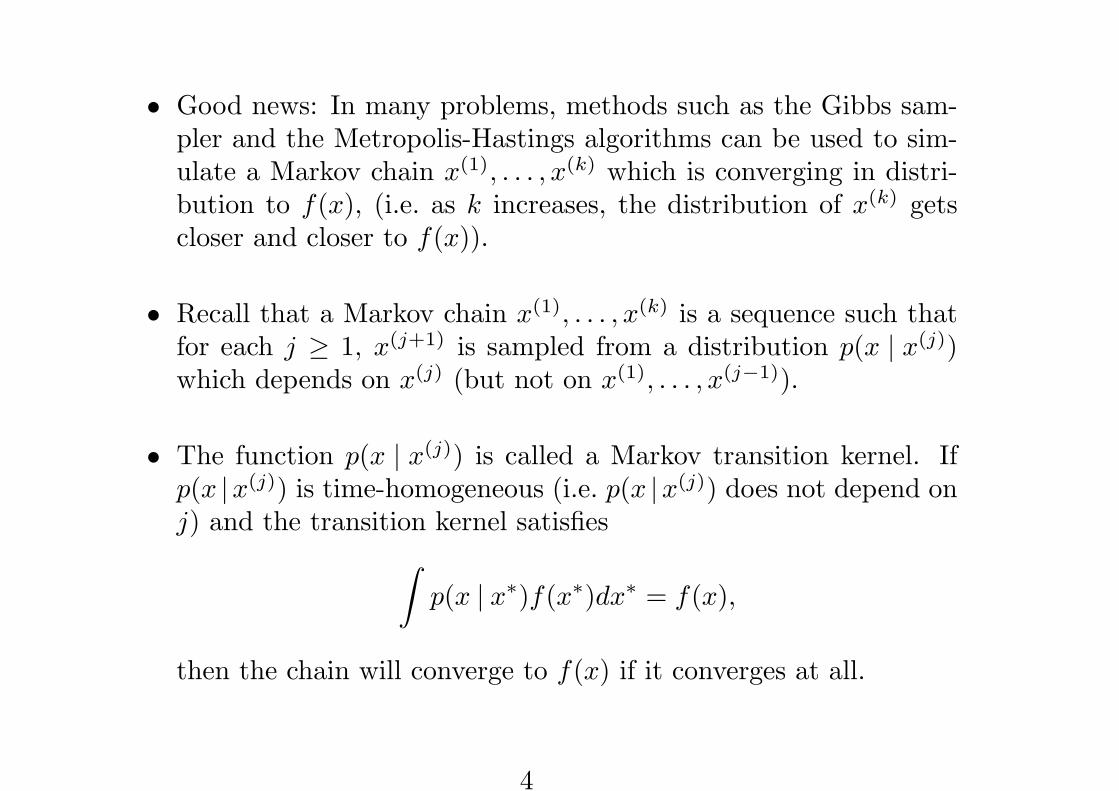
• Good news: In many problems, methods such as the Gibbs sam-pler and the Metropolis-Hastings algorithms can be used to sim-ulate a Markov chain x(1), . . . , x(k) which is converging in distri-bution to f(x), (i.e. as k increases, the distribution of x(k) getscloser and closer to f(x)).
• Recall that a Markov chain x(1), . . . , x(k) is a sequence such thatfor each j ≥ 1, x(j+1) is sampled from a distribution p(x | x(j))which depends on x(j) (but not on x(1), . . . , x(j−1)).
• The function p(x | x(j)) is called a Markov transition kernel. Ifp(x |x(j)) is time-homogeneous (i.e. p(x |x(j)) does not depend onj) and the transition kernel satisfies
∫p(x | x∗)f(x∗)dx∗ = f(x),
then the chain will converge to f(x) if it converges at all.
4
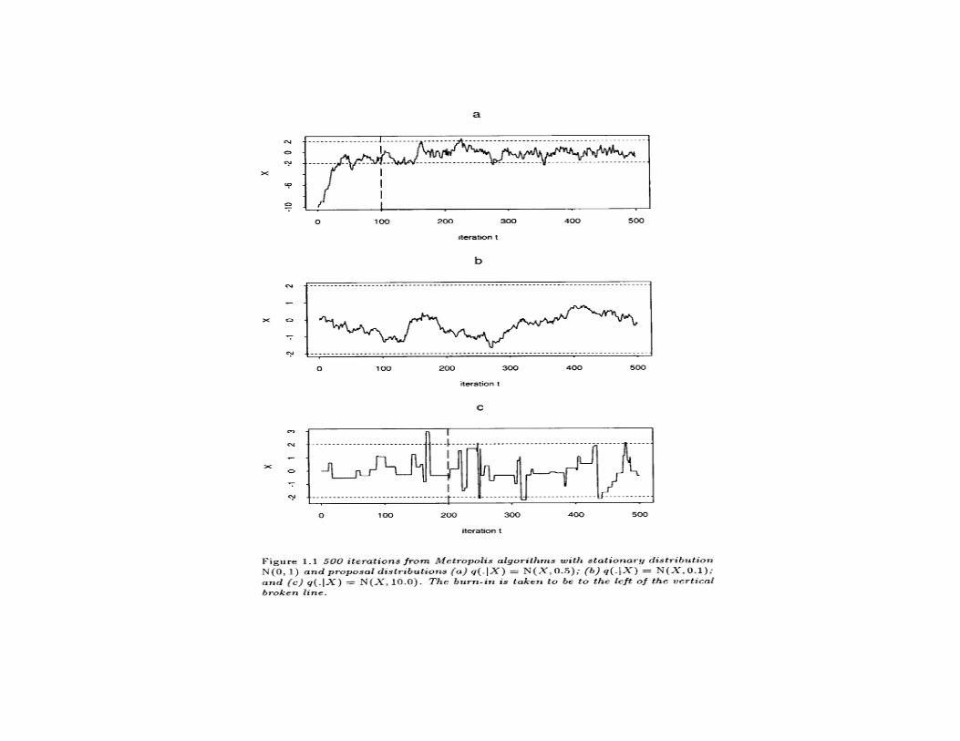
• Simulation of a Markov chain requires a starting value x(0). If thechain is converging to f(x), then the dependence between x(j) andx(0) diminishes as j increases. After a suitable “burn in” periodof l iterations, x(l), . . . , x(k) behaves like a dependent sample fromf(x).
• Such behavior is illustrated by Figure 1.1 on page 6 of Gilks,Richardson & Spieglehalter (1995).
• The output from such simulated chains can be used to estimatethe characteristics of f(x). For example, one can obtain approxi-mate iid samples of size m by taking the final x(k) values from mseparate chains.
• It is probably more efficient, however, to use all the simulatedvalues. For example, x1 = 1
k
∑j x
(j)1 will still converge to the
mean of x1.
5
• MCMC is the general procedure of simulating such Markov chainsand using them to draw inference about the characteristics of f(x).
• Methods which have ignited MCMC are the Gibbs sampler andthe more general Metropolis-Hastings algorithms. As will we nowsee, these are simply prescriptions for constructing a Markov tran-sition kernel p(x|x∗) which generates a Markov chain x(1), . . . , x(k)
converging to f(x).
2. The Gibbs Sampler (GS)
• The GS is an algorithm for simulating a Markov chain x(1), . . . , x(k)
which is converging to f(x), by successively sampling from the fullconditional component distributions f(xi|x−i), i = 1, . . . , p, wherex−i denotes the components of x other than xi.
6
• For simplicity, consider the case where p = 2. The GS generatesa Markov chain
(x(1)1 , x
(1)2 ), (x(2)
1 , x(2)2 ), . . . , (x(k)
1 , x(k)2 )
converging to f(x1, x2), by successively sampling
x(1)1 from f(x1 | x(0)
2 )
x(1)2 from f(x2 | x(1)
1 )
x(2)1 from f(x1 | x(1)
2 )...
x(k)1 from f(x1 | x(k−1)
2 )
x(k)2 from f(x2 | x(k)
1 )
(To get started, prespecify an initial value for x(0)2 ).
7
• For example, suppose
f(x1, x2) ∝(
nx1
)xx1+α−1
2 (1− x2)n−x1+β−1
x1 = 0, 1, . . . , n, 0 ≤ x2 ≤ 1.
The GS proceeds by successively sampling from
f(x1 | x2) = Binomial(n, x2)f(x2 | x1) = Beta(x1 + α, n− x1 + β)
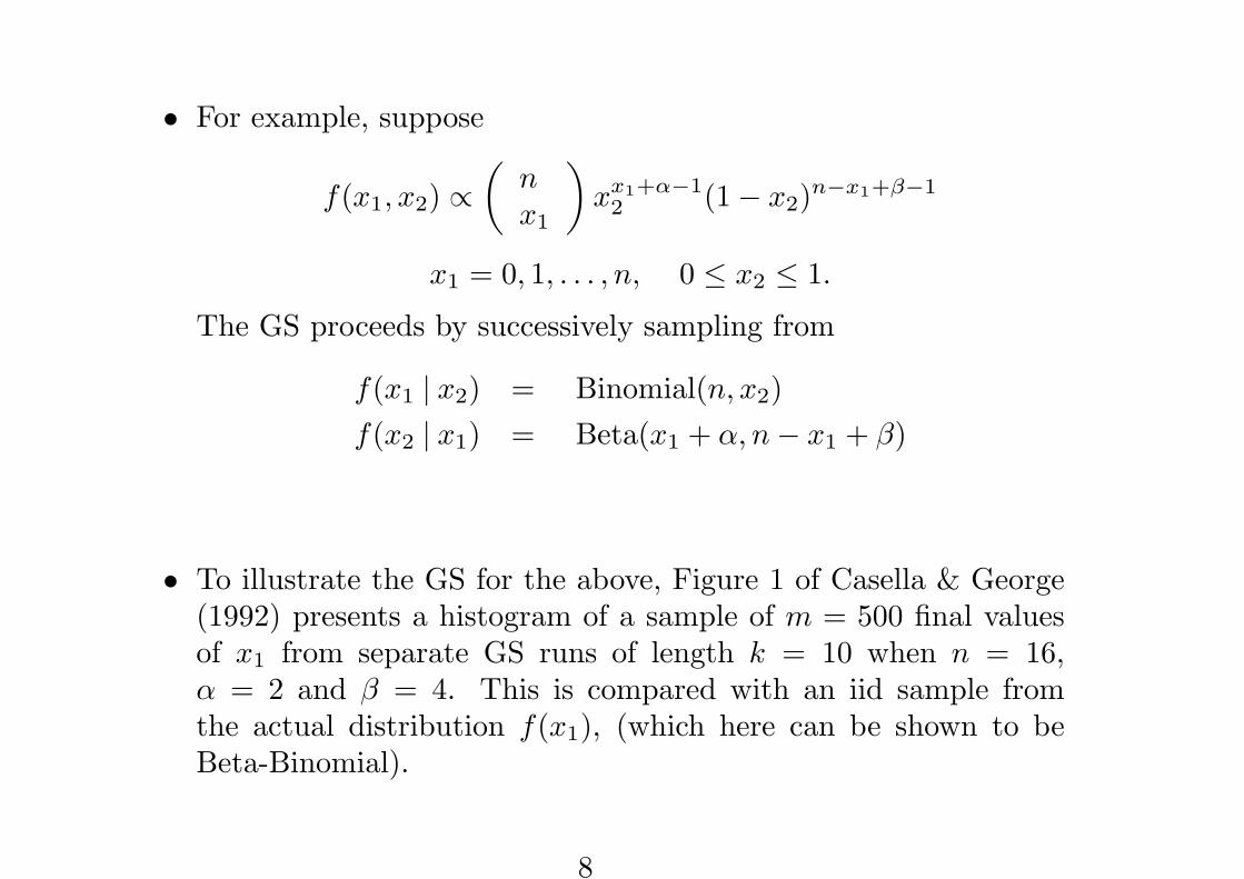
• To illustrate the GS for the above, Figure 1 of Casella & George(1992) presents a histogram of a sample of m = 500 final valuesof x1 from separate GS runs of length k = 10 when n = 16,α = 2 and β = 4. This is compared with an iid sample fromthe actual distribution f(x1), (which here can be shown to beBeta-Binomial).
8
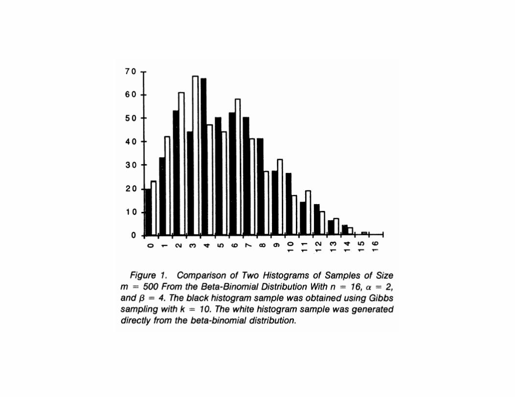

• Note that f(x1) =∫
f(x1, x2)dx2 =∫
f(x1 | x2)f(x2)dx2. Thisexpression suggests that an improved estimate of f(x1) in thisexample can be obtained by inserting the m values of x
(k)2 into
f(x1) =1m
m∑
i=1
f(x1 | x(i)2 ).
Figure 3 of Casella & George (1992) illustrates the improvementobtained by this estimate.
• Note that the conditional distributions for the above setup, theBinomial and the Beta, can be simulated by routine methods.This is not always the case. For example, f(x1 | x2) from page2 is not of standard form. Fortunately, such distributions can besimulated using envelope methods such as rejection sampling, theratio-of-uniforms method or adaptive rejection resampling. Aswe’ll see, Metropolis-Hastings algorithms can also be used for thispurpose.
9
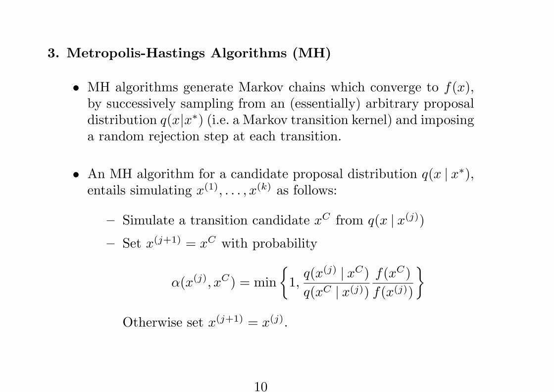
3. Metropolis-Hastings Algorithms (MH)
• MH algorithms generate Markov chains which converge to f(x),by successively sampling from an (essentially) arbitrary proposaldistribution q(x|x∗) (i.e. a Markov transition kernel) and imposinga random rejection step at each transition.
• An MH algorithm for a candidate proposal distribution q(x | x∗),entails simulating x(1), . . . , x(k) as follows:
– Simulate a transition candidate xC from q(x | x(j))
– Set x(j+1) = xC with probability
α(x(j), xC) = min{
1,q(x(j) | xC)q(xC | x(j))
f(xC)f(x(j))
}
Otherwise set x(j+1) = x(j).
10
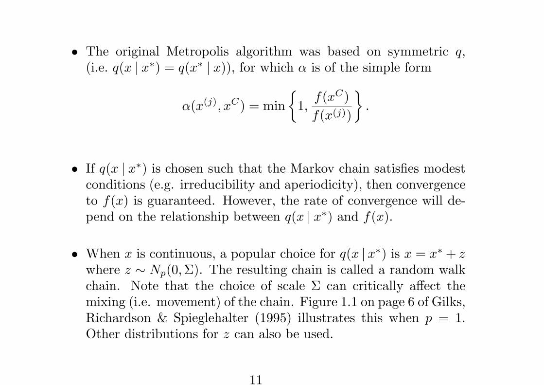
• The original Metropolis algorithm was based on symmetric q,(i.e. q(x | x∗) = q(x∗ | x)), for which α is of the simple form
α(x(j), xC) = min{
1,f(xC)f(x(j))
}.
• If q(x | x∗) is chosen such that the Markov chain satisfies modestconditions (e.g. irreducibility and aperiodicity), then convergenceto f(x) is guaranteed. However, the rate of convergence will de-pend on the relationship between q(x | x∗) and f(x).
• When x is continuous, a popular choice for q(x | x∗) is x = x∗ + zwhere z ∼ Np(0, Σ). The resulting chain is called a random walkchain. Note that the choice of scale Σ can critically affect themixing (i.e. movement) of the chain. Figure 1.1 on page 6 of Gilks,Richardson & Spieglehalter (1995) illustrates this when p = 1.Other distributions for z can also be used.
11

• Another useful choice, called an independence sampler, is obtainedwhen the proposal q(x | x∗) = q(x) does not depend on x∗. Theresulting α is of the form
α(x(j), xC) = min{
1,q(x(j))q(xC)
f(xC)f(x(j))
}.
Such samplers work well when q(x) is a good heavy-tailed approx-imation to f(x).
• It may be preferable to use an MH algorithm which updates thecomponents x
(j)i of x one at a time. It can shown that the Gibbs
sampler is just a special case of such a single-component MH al-gorithm where q is chosen so that α ≡ 1.
12

• Finally, to see why MH algorithms work, it is not too hard to showthat the implied transition kernel p(x | x∗) of any MH algorithmsatisfies
p(x | x∗)f(x∗) = p(x∗ | x)f(x),
a condition called detailed balance or reversibility. Integratingboth sides of this identity with respect to x∗ yields
∫p(x | x∗)f(x∗)dx∗ = f(x),
showing that f(x) is the limiting distribution when the chain con-verges.
4. The Model Liberation Movement
• Advances in computing technology have unleashed the power ofMonte Carlo methods, which in turn, are now unleashing the po-tential of statistical modeling.
13
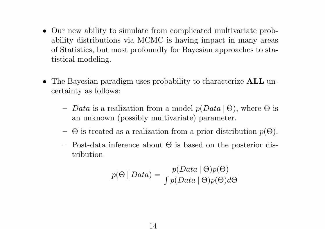
• Our new ability to simulate from complicated multivariate prob-ability distributions via MCMC is having impact in many areasof Statistics, but most profoundly for Bayesian approaches to sta-tistical modeling.
• The Bayesian paradigm uses probability to characterize ALL un-certainty as follows:
– Data is a realization from a model p(Data |Θ), where Θ isan unknown (possibly multivariate) parameter.
– Θ is treated as a realization from a prior distribution p(Θ).
– Post-data inference about Θ is based on the posterior dis-tribution
p(Θ |Data) =p(Data |Θ)p(Θ)∫p(Data |Θ)p(Θ)dΘ
14
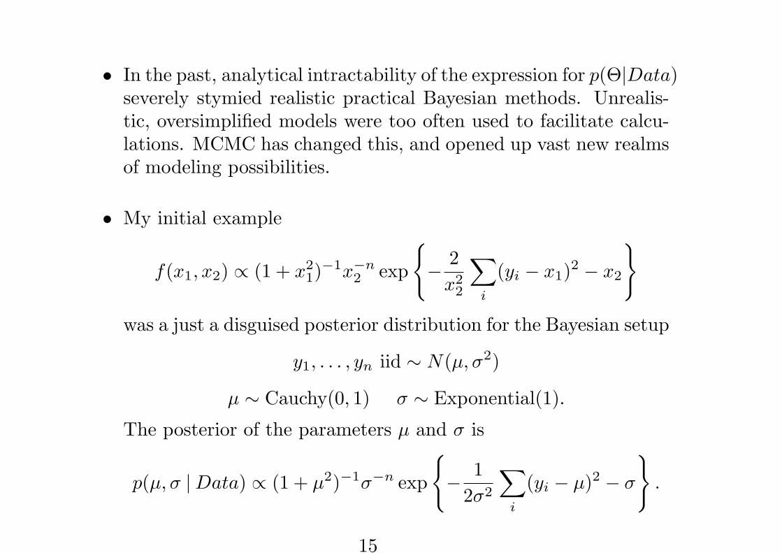
• In the past, analytical intractability of the expression for p(Θ|Data)severely stymied realistic practical Bayesian methods. Unrealis-tic, oversimplified models were too often used to facilitate calcu-lations. MCMC has changed this, and opened up vast new realmsof modeling possibilities.
• My initial example
f(x1, x2) ∝ (1 + x21)−1x−n
2 exp
{− 2
x22
∑
i
(yi − x1)2 − x2
}
was a just a disguised posterior distribution for the Bayesian setup
y1, . . . , yn iid ∼ N(µ, σ2)
µ ∼ Cauchy(0, 1) σ ∼ Exponential(1).
The posterior of the parameters µ and σ is
p(µ, σ |Data) ∝ (1 + µ2)−1σ−n exp
{− 1
2σ2
∑
i
(yi − µ)2 − σ
}.
15
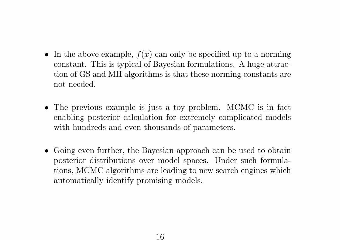
• In the above example, f(x) can only be specified up to a normingconstant. This is typical of Bayesian formulations. A huge attrac-tion of GS and MH algorithms is that these norming constants arenot needed.
• The previous example is just a toy problem. MCMC is in factenabling posterior calculation for extremely complicated modelswith hundreds and even thousands of parameters.
• Going even further, the Bayesian approach can be used to obtainposterior distributions over model spaces. Under such formula-tions, MCMC algorithms are leading to new search engines whichautomatically identify promising models.
16
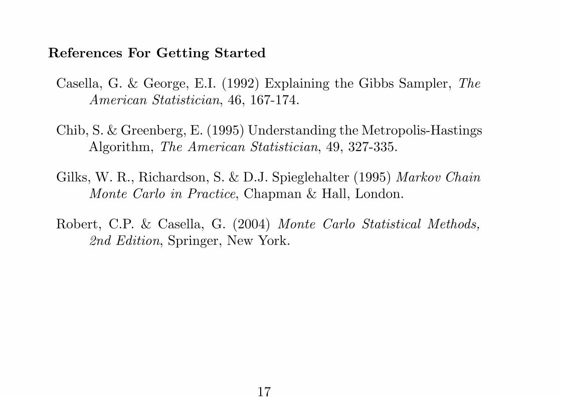
References For Getting Started
Casella, G. & George, E.I. (1992) Explaining the Gibbs Sampler, TheAmerican Statistician, 46, 167-174.
Chib, S. & Greenberg, E. (1995) Understanding the Metropolis-HastingsAlgorithm, The American Statistician, 49, 327-335.
Gilks, W. R., Richardson, S. & D.J. Spieglehalter (1995) Markov ChainMonte Carlo in Practice, Chapman & Hall, London.
Robert, C.P. & Casella, G. (2004) Monte Carlo Statistical Methods,2nd Edition, Springer, New York.
17
Lecture II
Bayesian Approaches for Model Uncertainty
Ed GeorgeUniversity of Pennsylvania
Seminaire de PrintempsVillars-sur-Ollon, Switzerland
March 2005
1
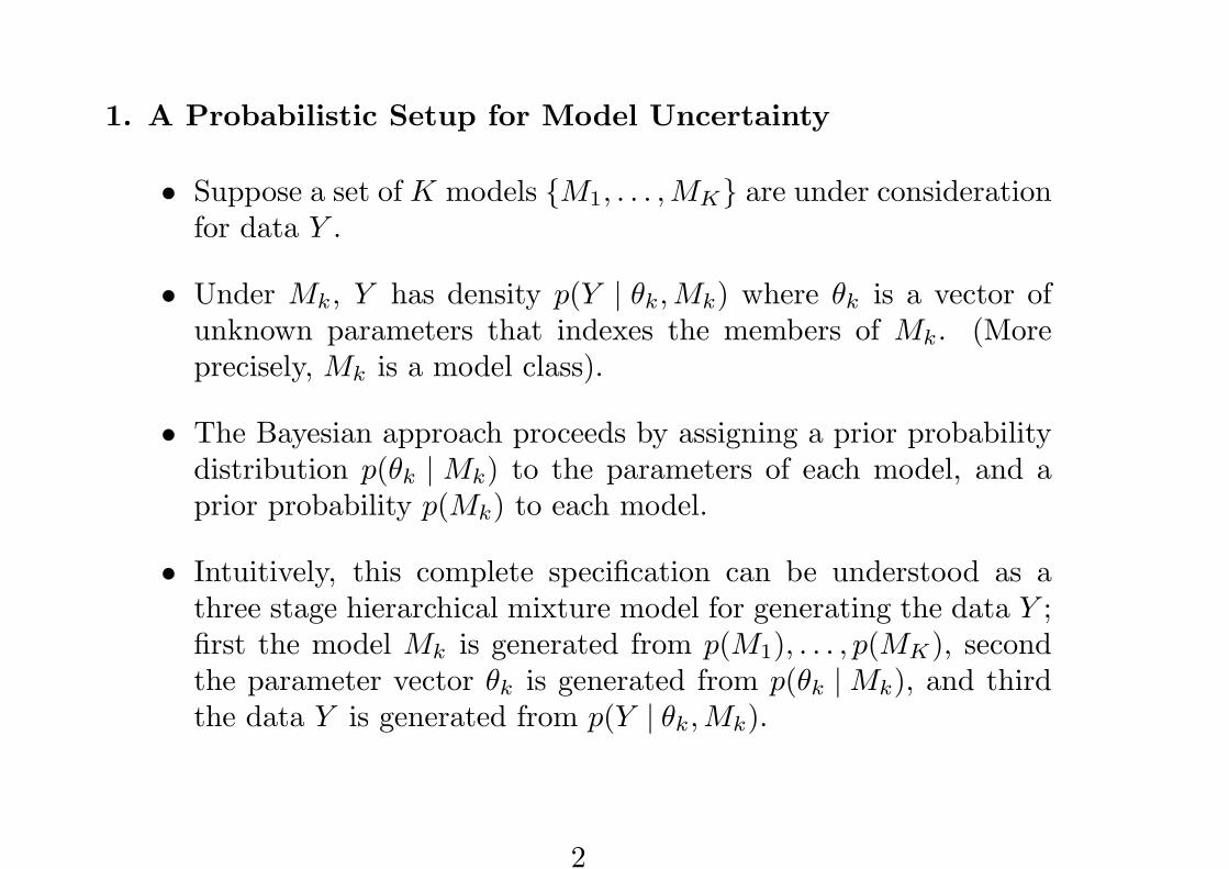
1. A Probabilistic Setup for Model Uncertainty
• Suppose a set of K models {M1, . . . , MK} are under considerationfor data Y .
• Under Mk, Y has density p(Y | θk,Mk) where θk is a vector ofunknown parameters that indexes the members of Mk. (Moreprecisely, Mk is a model class).
• The Bayesian approach proceeds by assigning a prior probabilitydistribution p(θk | Mk) to the parameters of each model, and aprior probability p(Mk) to each model.
• Intuitively, this complete specification can be understood as athree stage hierarchical mixture model for generating the data Y ;first the model Mk is generated from p(M1), . . . , p(MK), secondthe parameter vector θk is generated from p(θk |Mk), and thirdthe data Y is generated from p(Y | θk,Mk).
2
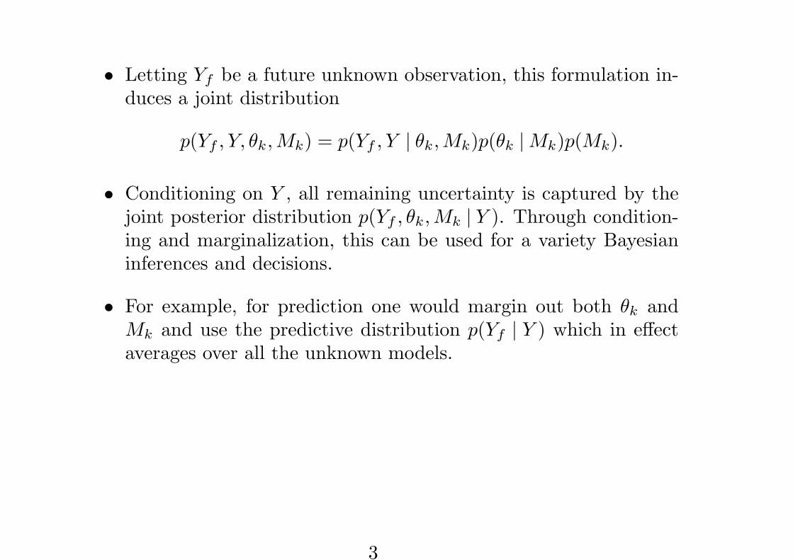
• Letting Yf be a future unknown observation, this formulation in-duces a joint distribution
p(Yf , Y, θk,Mk) = p(Yf , Y | θk,Mk)p(θk |Mk)p(Mk).
• Conditioning on Y , all remaining uncertainty is captured by thejoint posterior distribution p(Yf , θk, Mk | Y ). Through condition-ing and marginalization, this can be used for a variety Bayesianinferences and decisions.
• For example, for prediction one would margin out both θk andMk and use the predictive distribution p(Yf | Y ) which in effectaverages over all the unknown models.
3
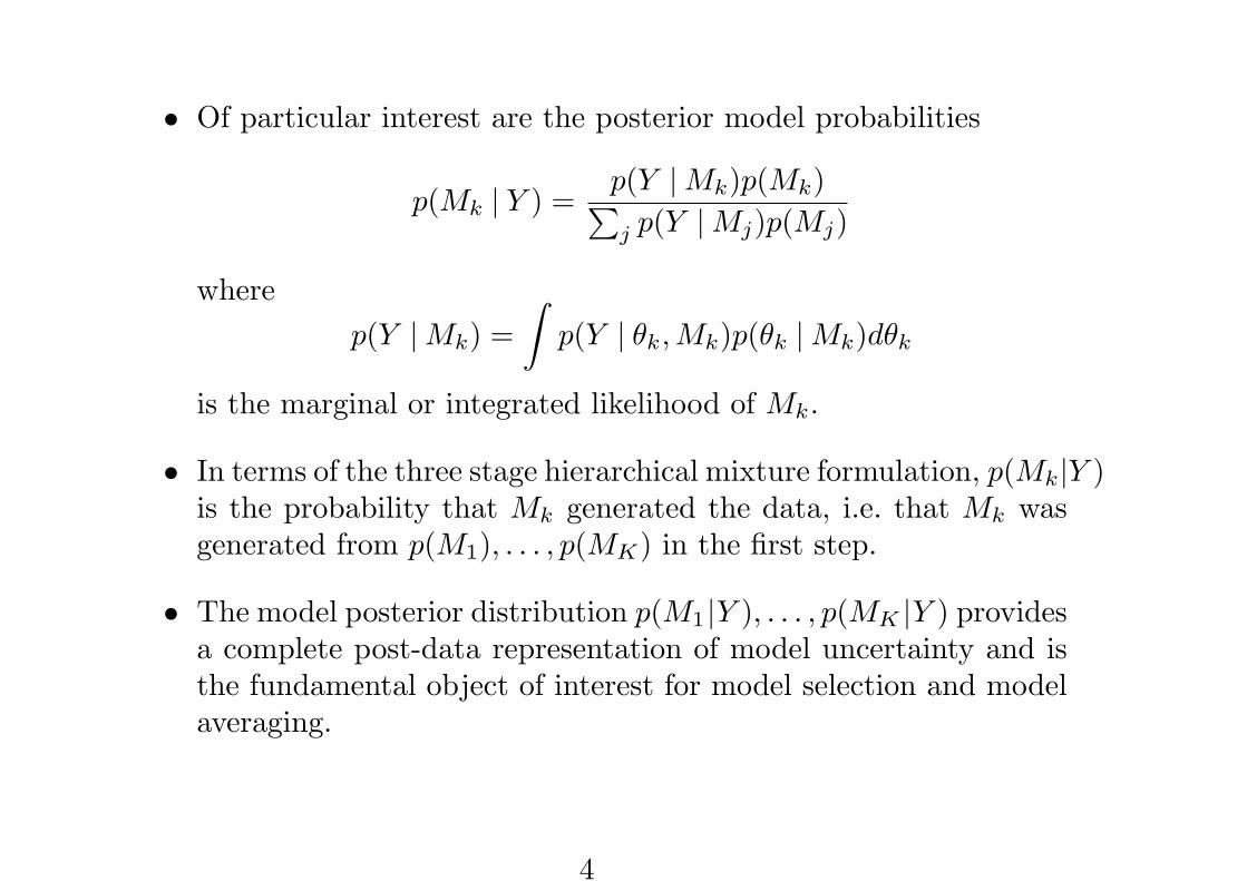
• Of particular interest are the posterior model probabilities
p(Mk | Y ) =p(Y |Mk)p(Mk)∑j p(Y |Mj)p(Mj)
wherep(Y |Mk) =
∫p(Y | θk, Mk)p(θk |Mk)dθk
is the marginal or integrated likelihood of Mk.
• In terms of the three stage hierarchical mixture formulation, p(Mk|Y )is the probability that Mk generated the data, i.e. that Mk wasgenerated from p(M1), . . . , p(MK) in the first step.
• The model posterior distribution p(M1 |Y ), . . . , p(MK |Y ) providesa complete post-data representation of model uncertainty and isthe fundamental object of interest for model selection and modelaveraging.
4
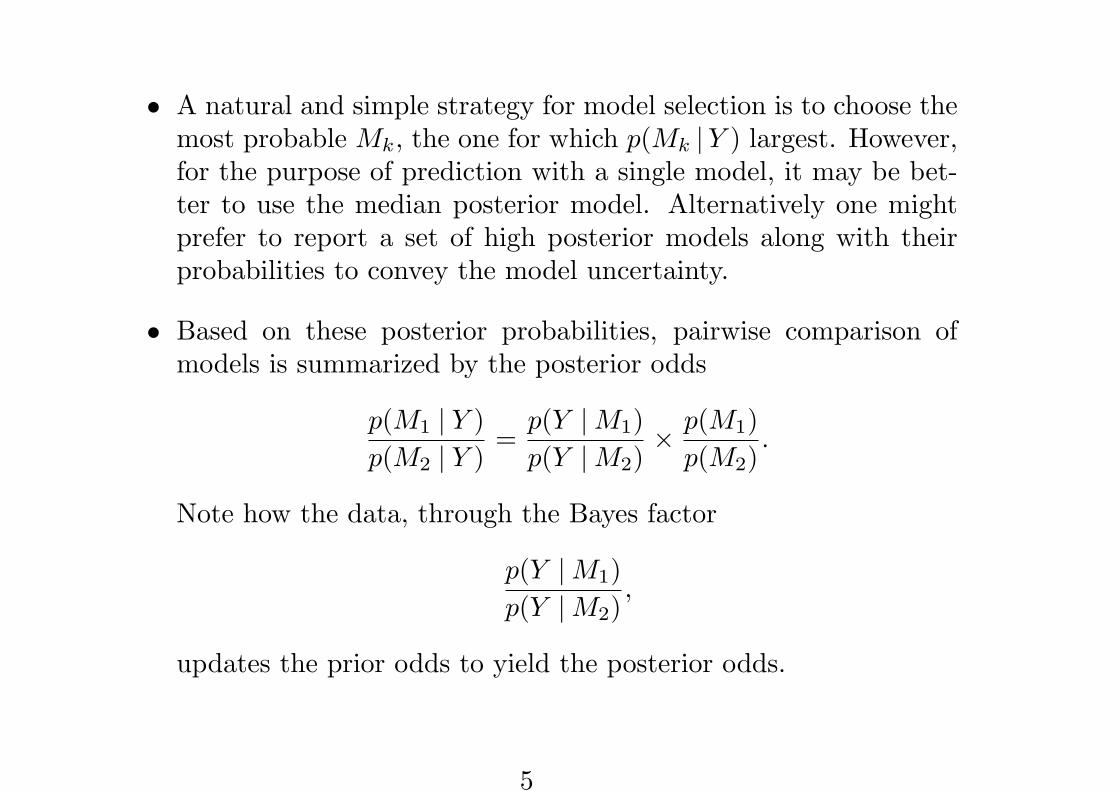
• A natural and simple strategy for model selection is to choose themost probable Mk, the one for which p(Mk |Y ) largest. However,for the purpose of prediction with a single model, it may be bet-ter to use the median posterior model. Alternatively one mightprefer to report a set of high posterior models along with theirprobabilities to convey the model uncertainty.
• Based on these posterior probabilities, pairwise comparison ofmodels is summarized by the posterior odds
p(M1 | Y )p(M2 | Y )
=p(Y |M1)p(Y |M2)
× p(M1)p(M2)
.
Note how the data, through the Bayes factor
p(Y |M1)p(Y |M2)
,
updates the prior odds to yield the posterior odds.
5
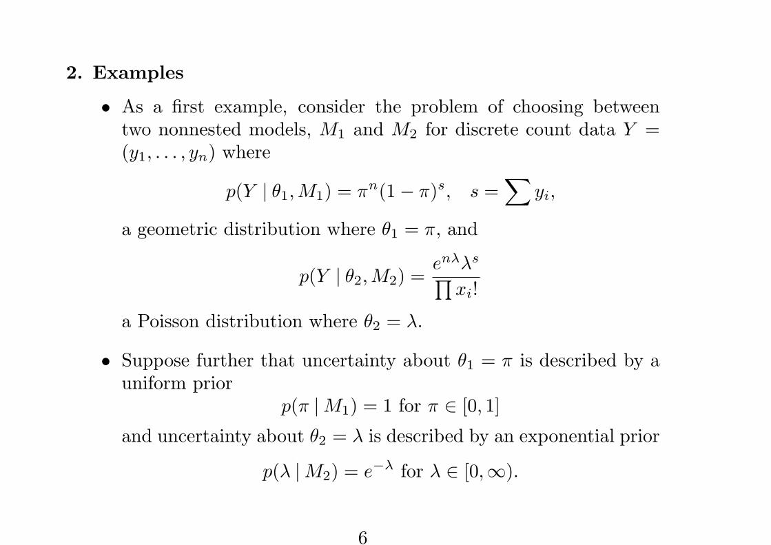
2. Examples
• As a first example, consider the problem of choosing betweentwo nonnested models, M1 and M2 for discrete count data Y =(y1, . . . , yn) where
p(Y | θ1,M1) = πn(1− π)s, s =∑
yi,
a geometric distribution where θ1 = π, and
p(Y | θ2, M2) =enλλs
∏xi!
a Poisson distribution where θ2 = λ.
• Suppose further that uncertainty about θ1 = π is described by auniform prior
p(π |M1) = 1 for π ∈ [0, 1]
and uncertainty about θ2 = λ is described by an exponential prior
p(λ |M2) = e−λ for λ ∈ [0,∞).
6
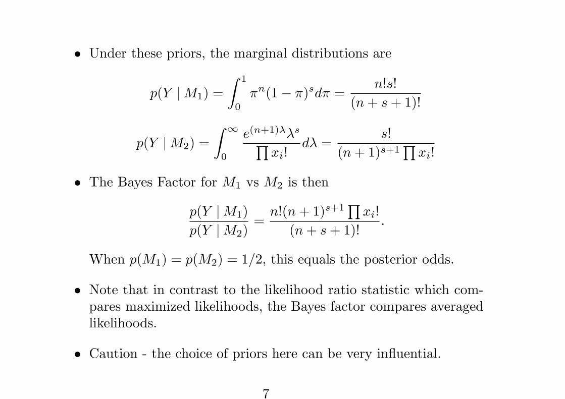
• Under these priors, the marginal distributions are
p(Y |M1) =∫ 1
0
πn(1− π)sdπ =n!s!
(n + s + 1)!
p(Y |M2) =∫ ∞
0
e(n+1)λλs
∏xi!
dλ =s!
(n + 1)s+1∏
xi!
• The Bayes Factor for M1 vs M2 is then
p(Y |M1)p(Y |M2)
=n!(n + 1)s+1
∏xi!
(n + s + 1)!.
When p(M1) = p(M2) = 1/2, this equals the posterior odds.
• Note that in contrast to the likelihood ratio statistic which com-pares maximized likelihoods, the Bayes factor compares averagedlikelihoods.
• Caution - the choice of priors here can be very influential.
7
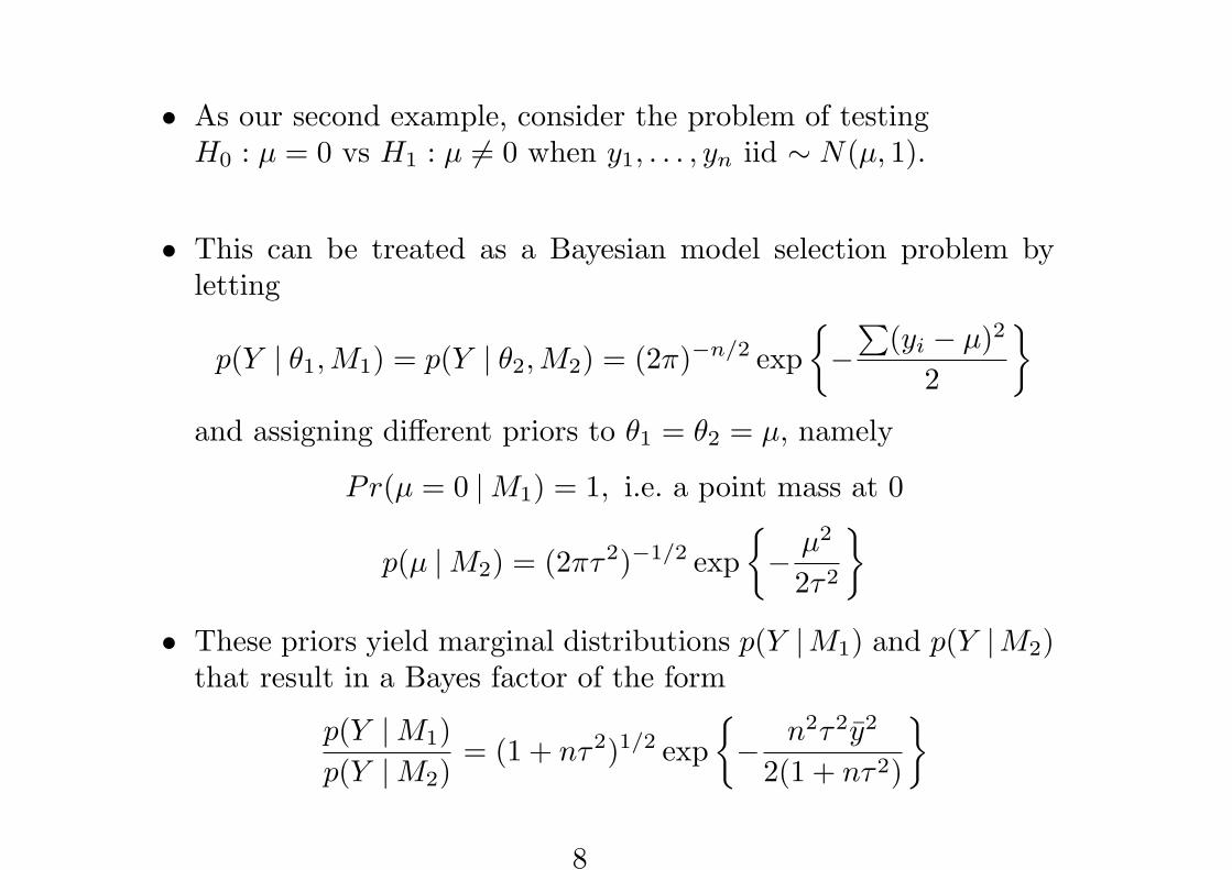
• As our second example, consider the problem of testingH0 : µ = 0 vs H1 : µ 6= 0 when y1, . . . , yn iid ∼ N(µ, 1).
• This can be treated as a Bayesian model selection problem byletting
p(Y | θ1, M1) = p(Y | θ2,M2) = (2π)−n/2 exp{−
∑(yi − µ)2
2
}
and assigning different priors to θ1 = θ2 = µ, namely
Pr(µ = 0 |M1) = 1, i.e. a point mass at 0
p(µ |M2) = (2πτ2)−1/2 exp{− µ2
2τ2
}
• These priors yield marginal distributions p(Y |M1) and p(Y |M2)that result in a Bayes factor of the form
p(Y |M1)p(Y |M2)
= (1 + nτ2)1/2 exp{− n2τ2y2
2(1 + nτ2)
}
8
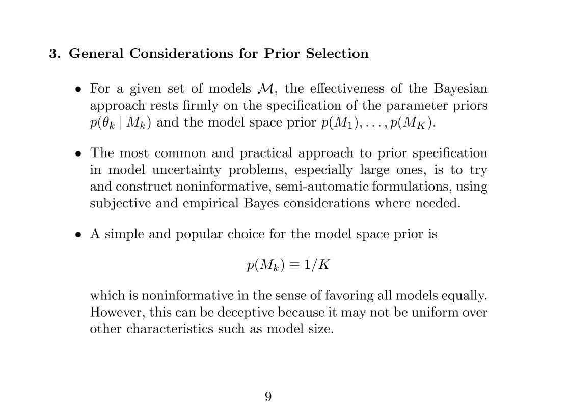
3. General Considerations for Prior Selection
• For a given set of models M, the effectiveness of the Bayesianapproach rests firmly on the specification of the parameter priorsp(θk |Mk) and the model space prior p(M1), . . . , p(MK).
• The most common and practical approach to prior specificationin model uncertainty problems, especially large ones, is to tryand construct noninformative, semi-automatic formulations, usingsubjective and empirical Bayes considerations where needed.
• A simple and popular choice for the model space prior is
p(Mk) ≡ 1/K
which is noninformative in the sense of favoring all models equally.However, this can be deceptive because it may not be uniform overother characteristics such as model size.
9
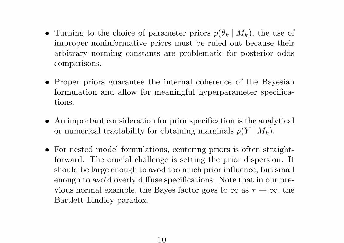
• Turning to the choice of parameter priors p(θk | Mk), the use ofimproper noninformative priors must be ruled out because theirarbitrary norming constants are problematic for posterior oddscomparisons.
• Proper priors guarantee the internal coherence of the Bayesianformulation and allow for meaningful hyperparameter specifica-tions.
• An important consideration for prior specification is the analyticalor numerical tractability for obtaining marginals p(Y |Mk).
• For nested model formulations, centering priors is often straight-forward. The crucial challenge is setting the prior dispersion. Itshould be large enough to avod too much prior influence, but smallenough to avoid overly diffuse specifications. Note that in our pre-vious normal example, the Bayes factor goes to ∞ as τ →∞, theBartlett-Lindley paradox.
10
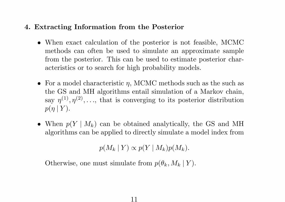
4. Extracting Information from the Posterior
• When exact calculation of the posterior is not feasible, MCMCmethods can often be used to simulate an approximate samplefrom the posterior. This can be used to estimate posterior char-acteristics or to search for high probability models.
• For a model characteristic η, MCMC methods such as the such asthe GS and MH algorithms entail simulation of a Markov chain,say η(1), η(2), . . ., that is converging to its posterior distributionp(η | Y ).
• When p(Y | Mk) can be obtained analytically, the GS and MHalgorithms can be applied to directly simulate a model index from
p(Mk | Y ) ∝ p(Y |Mk)p(Mk).
Otherwise, one must simulate from p(θk,Mk | Y ).
11
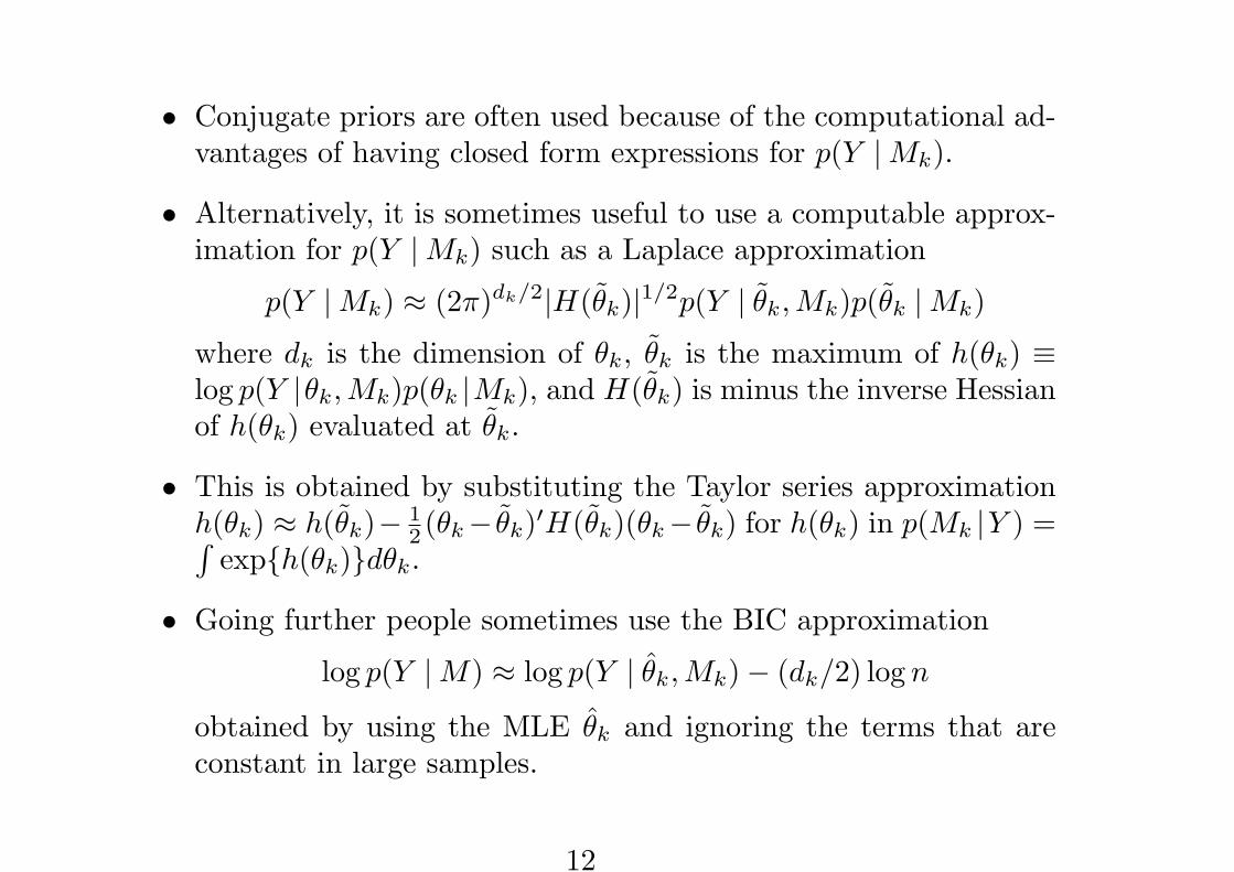
• Conjugate priors are often used because of the computational ad-vantages of having closed form expressions for p(Y |Mk).
• Alternatively, it is sometimes useful to use a computable approx-imation for p(Y |Mk) such as a Laplace approximation
p(Y |Mk) ≈ (2π)dk/2|H(θk)|1/2p(Y | θk,Mk)p(θk |Mk)
where dk is the dimension of θk, θk is the maximum of h(θk) ≡log p(Y |θk, Mk)p(θk |Mk), and H(θk) is minus the inverse Hessianof h(θk) evaluated at θk.
• This is obtained by substituting the Taylor series approximationh(θk) ≈ h(θk)− 1
2 (θk− θk)′H(θk)(θk− θk) for h(θk) in p(Mk |Y ) =∫exp{h(θk)}dθk.
• Going further people sometimes use the BIC approximation
log p(Y |M) ≈ log p(Y | θk,Mk)− (dk/2) log n
obtained by using the MLE θk and ignoring the terms that areconstant in large samples.
12
References For Getting Started
Chipman, H., George, E.I. and McCulloch, R.E. (2001). The PracticalImplementation of Bayesian Model Selection (with discussion). InModel Selection (P. Lahiri, ed.) IMS Lecture Notes – MonographSeries, Volume 38, 65-134.
Clyde, M. & George, E.I. (2004). Model Uncertainty, Statistical Sci-ence, 19 1 81-94.
George, E.I. (1999). Bayesian Model Selection. In Encyclopedia ofStatistical Sciences, Update Volume 3, (eds. S. Kotz, C. Readand D. Banks), pp 39-46, Wiley, N.Y.
13
Lecture III
Bayesian Variable Selection
Ed GeorgeUniversity of Pennsylvania
Seminaire de PrintempsVillars-sur-Ollon, Switzerland
March 2005
1
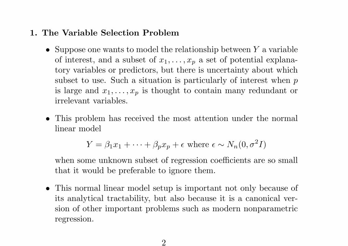
1. The Variable Selection Problem
• Suppose one wants to model the relationship between Y a variableof interest, and a subset of x1, . . . , xp a set of potential explana-tory variables or predictors, but there is uncertainty about whichsubset to use. Such a situation is particularly of interest when pis large and x1, . . . , xp is thought to contain many redundant orirrelevant variables.
• This problem has received the most attention under the normallinear model
Y = β1x1 + · · ·+ βpxp + ε where ε ∼ Nn(0, σ2I)
when some unknown subset of regression coefficients are so smallthat it would be preferable to ignore them.
• This normal linear model setup is important not only because ofits analytical tractability, but also because it is a canonical ver-sion of other important problems such as modern nonparametricregression.
2
• It will be convenient here to index each of the 2p possible subsetchoices by
γ = (γ1, . . . , γp)′,
where γi = 0 or 1 according to whether βi is small or large, re-spectively. The size of the γth subset is denoted qγ ≡ γ′1. Werefer to γ as a model since it plays the same role as Mk describedin Lecture II.
2. Model Space Priors for Variable Selection
• For the specification of the model space prior, most Bayesian vari-able selection implementations have used independence priors ofthe form
p(γ) =∏
wγi
i (1− wi)1−γi .
• Under this prior, each xi enters the model independently withprobability p(γi = 1) = 1− p(γi = 0) = wi.
3
• A useful simplification of this yields
p(γ) = wqγ (1− w)p−qγ ,
where w is the expected proportion of x′is in the model. A specialcase being the popular uniform prior
p(γ) ≡ 1/2p.
Note that both of these priors are informative about the size ofthe model.
• Related priors that might also be considered are
p(γ) =B(α + qγ , β + p− qγ)
B(α, β)
obtained putting a Beta prior on w, and more generally
p(γ) =(
pqγ
)−1
h(qγ)
obtained by putting a prior h(qγ) on the model size.
4
3. Parameter Priors for Selection of Nonzero βi
• When the goal is to ignore only those xi for which βi = 0, theproblem then becomes that of selecting a submodel of the form
Y = Xγβγ + ε, ε ∼ Nn(0, σ2I)
where Xγ is the n x qγ matrix whose columns correspond to theγth subset of x1, . . . , xp and βγ is a qγ × 1 vector of unknownregression coefficients. Here, (βγ , σ2) plays the role of θk describedin Lecture II.
• Perhaps the most commonly applied parameter prior form for thissetup is the conjugate normal-inverse-gamma prior
p(βγ | σ2, γ) = Nqγ (0, σ2Σγ),
p(σ2 | γ) = p(σ2) = IG(ν/2, νλ/2).
(p(σ2) here is equivalent to νλ/σ2 ∼ χ2ν).
5
• A valuable feature of this prior is its analytical tractability; βγ
and σ2 can be eliminated by routine integration to yield
p(Y | γ) ∝ |X ′γXγ + Σ−1
γ |−1/2|Σγ |−1/2(νλ + S2γ)−(n+ν)/2
whereS2
γ = Y ′Y − Y ′Xγ(X ′γXγ + Σ−1
γ )−1X ′γY.
The use of these closed form expressions can substantially speedup posterior evaluation and MCMC exploration, as we will see.
• In choosing values for the hyperparameters that control p(σ2), λmay be thought of as a prior estimate of σ2, and ν may be thoughtof as the prior sample size associated with this estimate.
• Let σ2FULL and σ2
Y denote the traditional estimates of σ2 based onthe saturated and null models respectively. Treating σ2
FULL andσ2
Y as rough under- and over-estimates of σ2, one might choose λand ν so that p(σ2) assigns substantial probability to the interval(σ2
FULL, σ2Y ). This should at least avoid gross misspecification.
6
• Alternatively, the explicit choice of λ and ν can be avoided byusing p(σ2) ∝ 1/σ2, the limit of the inverse-gamma prior as ν → 0.
• For choosing the prior covariance matrix Σγ that controls p(βγ |σ2, γ),specification is substantially simplified by setting Σγ = c Vγ , wherec is a scalar and Vγ is a preset form such as Vγ = (X ′
γXγ)−1 orVγ = Iqγ , the qγ × qγ identity matrix.
• Having fixed Vγ , the goal is then to choose c large enough so thatp(βγ | σ2, γ) is relatively flat over the region of plausible valuesof βγ , thereby reducing prior influence. At the same time it isimportant to avoid excessively large values of c because the Bayesfactors will eventually put increasing weight on the null model asc → ∞, the Bartlett-Lindley paradox. For practical purposes, arough guide is to choose c so that p(βγ | σ2, γ) assigns substantialprobability to the range of all plausible values for βγ . Choices ofc between 10 and 10,000 seem to yield good results.
7
4. Posterior Calculation and Exploration
• The previous conjugate prior formulations allow for analyticalmargining out of β and σ2 from p(Y, β, σ2 | γ) to yield a com-putable, closed form expression
g(γ) ∝ p(Y | γ)p(γ) ∝ p(γ | Y )
that can greatly facilitate posterior calculation and exploration.
• For example, when Σγ = c (X ′γXγ)−1, we can obtain
g(γ) = (1 + c)−qγ/2(νλ + Y ′Y − (1 + 1/c)−1W ′W )−(n+ν)/2p(γ)
where W = T ′−1X ′γY for upper triangular T such that T ′T =
X ′γXγ (obtainable by the Cholesky decomposition). This repre-
sentation allows for fast updating of T , and hence W and g(γ),when γ is changed one component at a time, requiring O(q2
γ) op-erations per update, where γ is the changed value.
8
• The availability of g(γ) ∝ p(γ |Y ) allows for the flexible construc-tion of MCMC algorithms that simulate a Markov chain
γ(1), γ(2), γ(3), . . .
converging (in distribution) to p(γ | Y ).
• A variety of such MCMC algorithms can be conveniently obtainedby applying the GS with g(γ). For example, by generating eachγ component from the full conditionals
p(γi | γ(i), Y )
(γ(i) = {γj : j 6= i}) where the γi may be drawn in any fixed orrandom order.
• The generation of such components can be obtained rapidly as asequence of Bernoulli draws using simple functions of the ratio
p(γi = 1, γ(i) | Y )p(γi = 0, γ(i) | Y )
=g(γi = 1, γ(i))g(γi = 0, γ(i))
.
9
• Such g(γ) also facilitates the use of MH algorithms. Becauseg(γ)/g(γ′) = p(γ | Y )/p(γ′ | Y ), these are of the form:
1. Simulate a candidate γ∗ from a transition kernel q(γ∗ |γ(j)).
2. Set γ(j+1) = γ∗ with probability
α(γ∗ | γ(j)) = min{
q(γ(j) | γ∗)q(γ∗ | γ(j))
g(γ∗)g(γ(j))
, 1}
. (1)
Otherwise, γ(j+1) = γ(j).
• A useful class of MH algorithms, the Metropolis algorithms, areobtained from the class of symmetric transition kernels of the form
q(γ1 | γ0) = qd ifp∑1
|γ0i − γ1
i | = d. (2)
which simulate a candidate γ∗ by randomly changing d compo-nents of γ(j) with probability qd.
10
• When available, fast updating schemes for g(γ) can be exploitedin all these MCMC algorithms.
5. Extracting Information from the Output
• The simulated Markov chain sample γ(1), . . . , γ(K) contains valu-able information about the posterior p(γ | Y ).
• Empirical frequencies provide consistent estimates of individualmodel probabilities or characteristics such as p(βi 6= 0 | Y ).
• When closed form g(γ) is available, we can do better. For exam-ple, the exact relative probability of any two values γ0 and γ1 isobtained as g(γ0) / g(γ1) in the sequence of simulated values.
11
• Such g(γ) also facilitates estimation of the normalizing constantp(γ |Y ) = Cg(γ). Let A be a preselected subset of γ values and letg(A) =
∑γ∈A g(γ) so that p(A | Y ) = C g(A). Then, a consistent
estimate of C is
C =1
g(A)K
K∑
k=1
IA(γ(k))
where IA( ) is the indicator of the set A.
• This yields improved estimates of the probability of individual γvalues
p(γ | Y ) = C g(γ),
as well as an estimate of the total visited probability
p(B | Y ) = C g(B),
where B is the set of visited γ values.
12
• The simulated γ(1), . . . , γ(K) can also play an important role inmodel averaging. For example, suppose one wanted to predict aquantity of interest ∆ by the posterior mean
E(∆ | Y ) =∑
all γ
E(∆ | γ, Y )p(γ | Y ).
When p is too large for exhaustive enumeration and p(γ | Y ) can-not be computed, E(∆ |Y ) is unavailable and is typically approx-imated by something of the form
E(∆ | Y ) =∑
γ∈S
E(∆ | γ, Y )p(γ | Y, S)
where S is a manageable subset of models and p(γ | Y, S) is aprobability distribution over S. (In some cases, E(∆ | γ, Y ) willalso need to be approximated).
13
• Letting S be the sampled values, a natural and consistent choicefor E(∆ | Y ) is
Ef (∆ | Y ) =∑
γ∈S
E(∆ | γ, Y )pf (γ | Y, S)
where pf (γ | Y, S) is the relative frequency of γ in S. However, itappears that when g(γ) is available, one can do better by using
Eg(∆ | Y ) =∑
γ∈S
E(∆ | γ, Y )pg(γ | Y, S)
where pg(γ | Y, S) = g(γ)/g(S) is the renormalized value of g(γ).
• For example, when S is an iid sample from p(γ | Y ), Eg(∆ | Y )approximates the best unbiased estimator of E(∆ |Y ) as the sam-ple size increases. To see this, note that when S is an iid sample,Ef (∆ | Y ) is unbiased for E(∆ | Y ). Since S (together with g)is sufficient, the Rao-Blackwellized estimator E(Ef (∆ | Y ) | S) isbest unbiased. But as the sample size increases, E(Ef (∆ | Y ) | S)→ Eg(∆ | Y ).
14
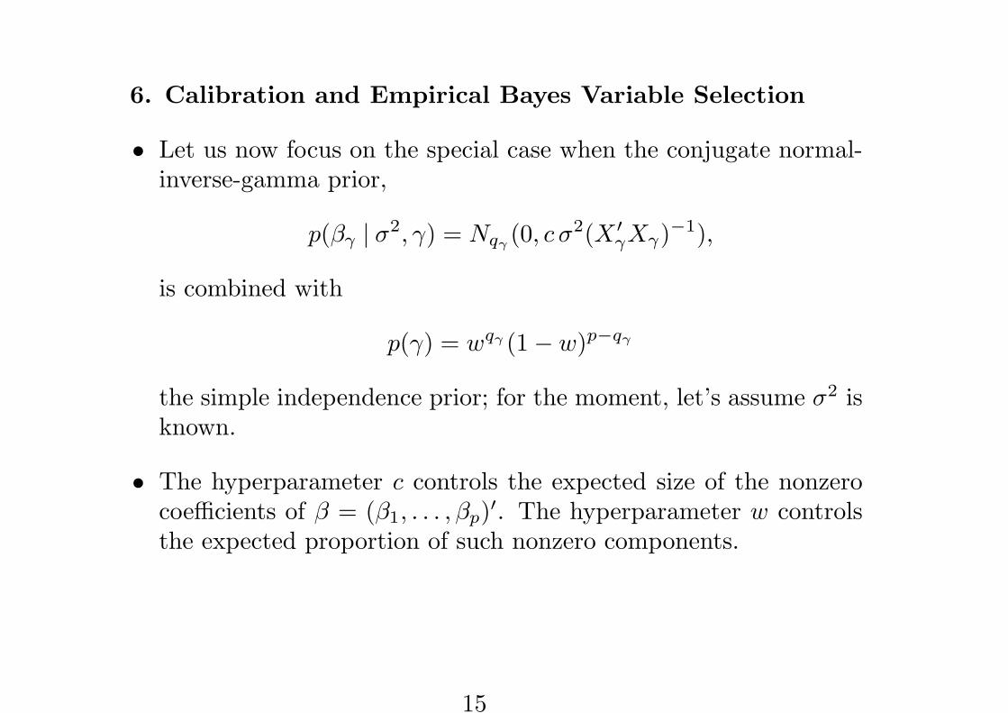
6. Calibration and Empirical Bayes Variable Selection
• Let us now focus on the special case when the conjugate normal-inverse-gamma prior,
p(βγ | σ2, γ) = Nqγ (0, c σ2(X ′γXγ)−1),
is combined with
p(γ) = wqγ (1− w)p−qγ
the simple independence prior; for the moment, let’s assume σ2 isknown.
• The hyperparameter c controls the expected size of the nonzerocoefficients of β = (β1, . . . , βp)′. The hyperparameter w controlsthe expected proportion of such nonzero components.
15
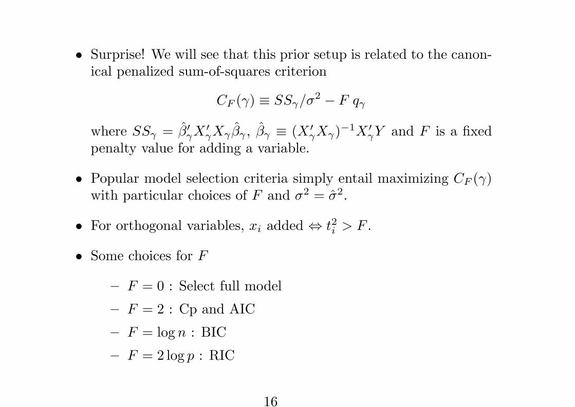
• Surprise! We will see that this prior setup is related to the canon-ical penalized sum-of-squares criterion
CF (γ) ≡ SSγ/σ2 − F qγ
where SSγ = β′γX ′γXγ βγ , βγ ≡ (X ′
γXγ)−1X ′γY and F is a fixed
penalty value for adding a variable.
• Popular model selection criteria simply entail maximizing CF (γ)with particular choices of F and σ2 = σ2.
• For orthogonal variables, xi added ⇔ t2i > F .
• Some choices for F
– F = 0 : Select full model
– F = 2 : Cp and AIC
– F = log n : BIC
– F = 2 log p : RIC
16
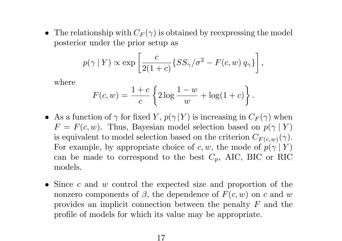
• The relationship with CF (γ) is obtained by reexpressing the modelposterior under the prior setup as
p(γ | Y ) ∝ exp[
c
2(1 + c){SSγ/σ2 − F (c, w) qγ}
],
where
F (c, w) =1 + c
c
{2 log
1− w
w+ log(1 + c)
}.
• As a function of γ for fixed Y , p(γ |Y ) is increasing in CF (γ) whenF = F (c, w). Thus, Bayesian model selection based on p(γ | Y )is equivalent to model selection based on the criterion CF (c,w)(γ).For example, by appropriate choice of c, w, the mode of p(γ | Y )can be made to correspond to the best Cp, AIC, BIC or RICmodels.
• Since c and w control the expected size and proportion of thenonzero components of β, the dependence of F (c, w) on c and wprovides an implicit connection between the penalty F and theprofile of models for which its value may be appropriate.
17
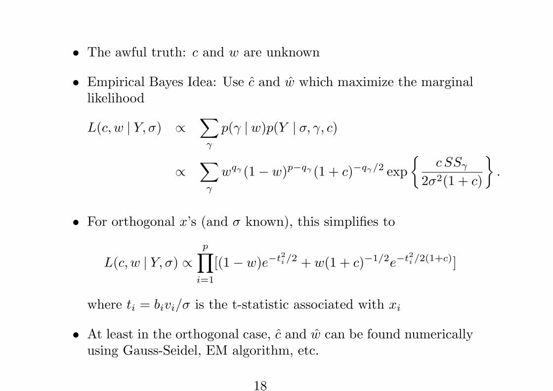
• The awful truth: c and w are unknown
• Empirical Bayes Idea: Use c and w which maximize the marginallikelihood
L(c, w | Y, σ) ∝∑
γ
p(γ | w)p(Y | σ, γ, c)
∝∑
γ
wqγ (1− w)p−qγ (1 + c)−qγ/2 exp{
c SSγ
2σ2(1 + c)
}.
• For orthogonal x’s (and σ known), this simplifies to
L(c, w | Y, σ) ∝p∏
i=1
[(1− w)e−t2i /2 + w(1 + c)−1/2e−t2i /2(1+c)]
where ti = bivi/σ is the t-statistic associated with xi
• At least in the orthogonal case, c and w can be found numericallyusing Gauss-Seidel, EM algorithm, etc.
18
• The best marginal maximum likelihood model is then the onewhich maximizes the “posterior” p(γ | Y, c, w, σ) or equivalently
CMML ≡ CF (c,w)
• In contrast to criteria of the form CF (γ) with prespecified fixedF , CMML uses an adaptive penalty F (c, w) that is implicitly basedon the estimated distribution of the regression coefficients.
• Estimating βγ after selecting γMML might then proceed using
E(βγ | Y, c, w, σ, γMML) =c
1 + cβγMML
• A computable conditional maximum likelihood approximation CCML
for the nonorthogonal case is available.
19
• Consider the simple model with X = I,
Y = β + ε where ε ∼ Nn(0, I)
where β = (β1, . . . , βp)′) is such that
β1, . . . , βq iid ∼ N(0, c)
βq+1, . . . , βp ≡ 0
• For p = n = 1000, and fixed values of c and q, simulated Y fromthe above model
• Evaluate γ by estimating
R(β, γ) ≡ Ec,q
∑
i
(YiI[xi ∈ γ]− βi)2
• Figures 1ab and 2 illustrate the adaptive advantages of the em-pirical Bayes selection criteria.
20
0 200 400 600 800 1000Nonzero Components
0
1000
2000
3000Lo
ssMMLCMLAIC/CpBICRICCBICMRIC
Figure 1(a). The average loss of the selection procedures when c = 25 and the number of nonzero components q = 0,10,25,50,100,200, 300, 400, 500, 750, 1000. We denote CMML by MML, CCML by CML, Cauchy BIC by CBIC and modified RIC by MRIC.

0 20 40 60 80 100Nonzero Components
0
100
200
300Lo
ssMMLCMLBICRIC/CBICMRIC
Figure 1(b). The average loss of the selection procedures when c = 25 and the number of nonzero components q = 0,10,25,50,100. We denote CMML by MML, CCML by CML, Cauchy BIC by CBIC and modified RIC by MRIC. RIC and CBIC are virtually identical here and so have been plotted together.
0 200 400 600 800 1000Nonzero Components
0
500
1000
1500
2000
2500
3000Lo
ssMMLCMLAIC/CpBICRICCBICMRIC
Figure 1(c). The average loss of the selection procedures when c = 5 and the number of nonzero components q = 0,10,25,50,100,200, 300, 400, 500, 750, 1000. We denote CMML by MML, CCML by CML, Cauchy BIC by CBIC and modified RIC by MRIC.
References For Getting Started
Chipman, H., George, E.I. and McCulloch, R.E. (2001). The PracticalImplementation of Bayesian Model Selection (with discussion). InModel Selection (P. Lahiri, ed.) IMS Lecture Notes – MonographSeries, Volume 38, 65-134.
George, E.I. and Foster, D.P. (2000) Calibration and empirical Bayesvariable selection. Biometrika 87, 731-748.
21
Lecture IV
High DimensionalPredictive Estimation
Ed GeorgeUniversity of Pennsylvania
Seminaire de PrintempsVillars-sur-Ollon, Switzerland
March 2005
1
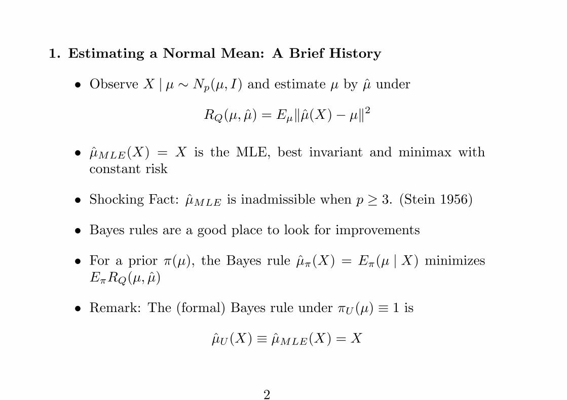
1. Estimating a Normal Mean: A Brief History
• Observe X | µ ∼ Np(µ, I) and estimate µ by µ under
RQ(µ, µ) = Eµ‖µ(X)− µ‖2
• µMLE(X) = X is the MLE, best invariant and minimax withconstant risk
• Shocking Fact: µMLE is inadmissible when p ≥ 3. (Stein 1956)
• Bayes rules are a good place to look for improvements
• For a prior π(µ), the Bayes rule µπ(X) = Eπ(µ | X) minimizesEπRQ(µ, µ)
• Remark: The (formal) Bayes rule under πU (µ) ≡ 1 is
µU (X) ≡ µMLE(X) = X
2
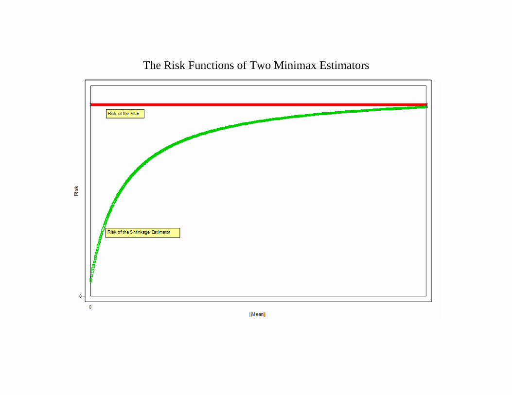
The Risk Functions of Two Minimax Estimators
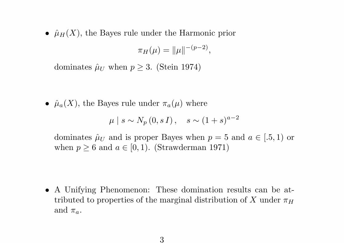
• µH(X), the Bayes rule under the Harmonic prior
πH(µ) = ‖µ‖−(p−2),
dominates µU when p ≥ 3. (Stein 1974)
• µa(X), the Bayes rule under πa(µ) where
µ | s ∼ Np (0, s I) , s ∼ (1 + s)a−2
dominates µU and is proper Bayes when p = 5 and a ∈ [.5, 1) orwhen p ≥ 6 and a ∈ [0, 1). (Strawderman 1971)
• A Unifying Phenomenon: These domination results can be at-tributed to properties of the marginal distribution of X under πH
and πa.
3
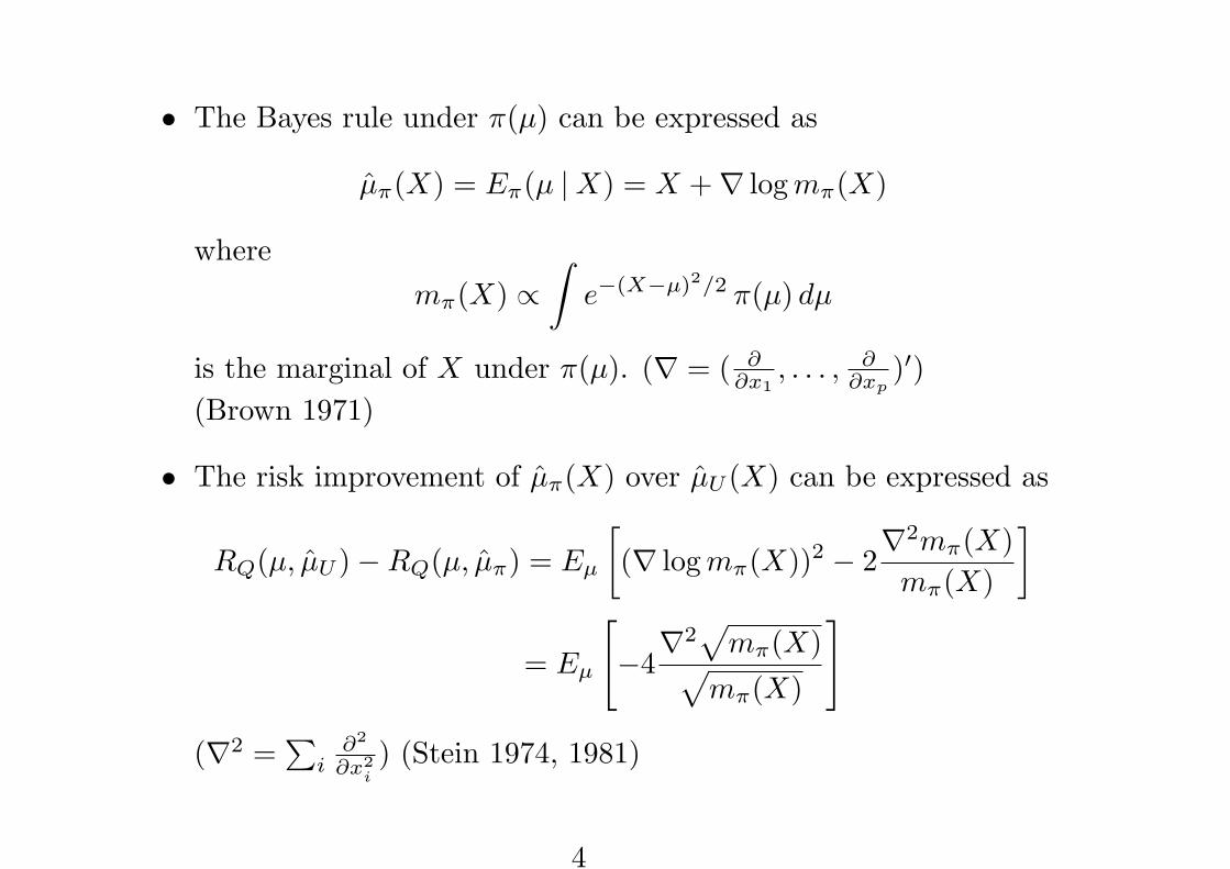
• The Bayes rule under π(µ) can be expressed as
µπ(X) = Eπ(µ |X) = X +∇ log mπ(X)
wheremπ(X) ∝
∫e−(X−µ)2/2 π(µ) dµ
is the marginal of X under π(µ). (∇ = ( ∂∂x1
, . . . , ∂∂xp
)′)(Brown 1971)
• The risk improvement of µπ(X) over µU (X) can be expressed as
RQ(µ, µU )−RQ(µ, µπ) = Eµ
[(∇ log mπ(X))2 − 2
∇2mπ(X)mπ(X)
]
= Eµ
[−4∇2
√mπ(X)√
mπ(X)
]
(∇2 =∑
i∂2
∂x2i
) (Stein 1974, 1981)
4
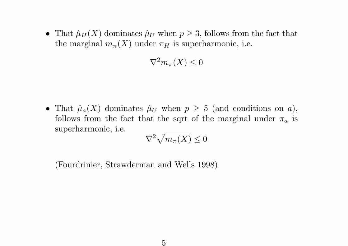
• That µH(X) dominates µU when p ≥ 3, follows from the fact thatthe marginal mπ(X) under πH is superharmonic, i.e.
∇2mπ(X) ≤ 0
• That µa(X) dominates µU when p ≥ 5 (and conditions on a),follows from the fact that the sqrt of the marginal under πa issuperharmonic, i.e.
∇2√
mπ(X) ≤ 0
(Fourdrinier, Strawderman and Wells 1998)
5
2. The Prediction Problem
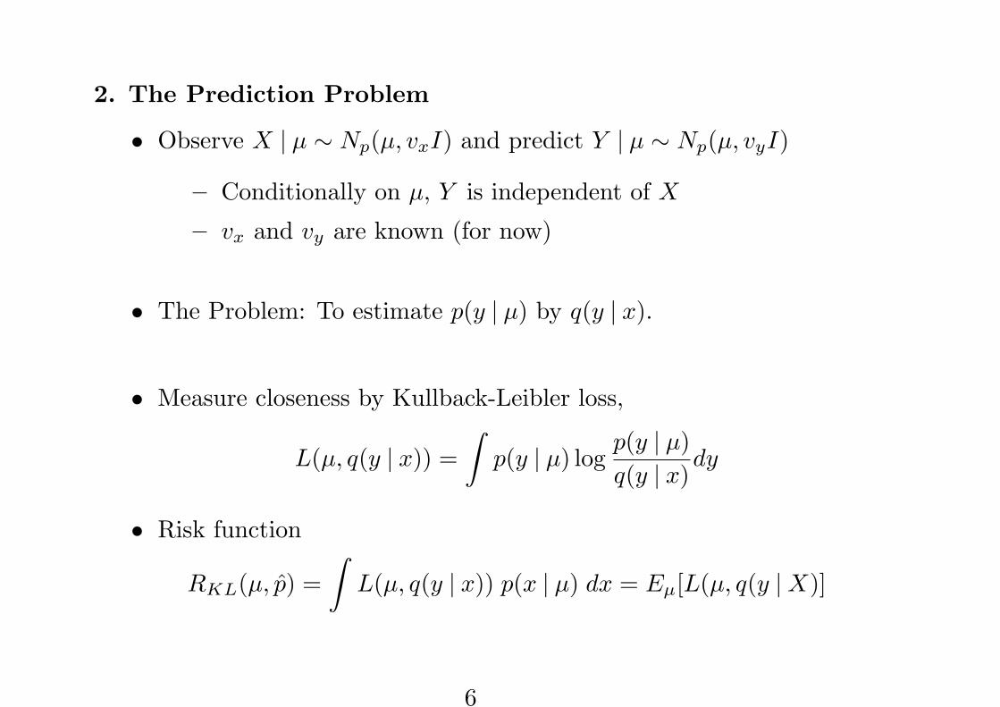
• Observe X | µ ∼ Np(µ, vxI) and predict Y | µ ∼ Np(µ, vyI)
– Conditionally on µ, Y is independent of X
– vx and vy are known (for now)
• The Problem: To estimate p(y | µ) by q(y | x).
• Measure closeness by Kullback-Leibler loss,
L(µ, q(y | x)) =∫
p(y | µ) logp(y | µ)q(y | x)
dy
• Risk function
RKL(µ, p) =∫
L(µ, q(y | x)) p(x | µ) dx = Eµ[L(µ, q(y |X)]
6
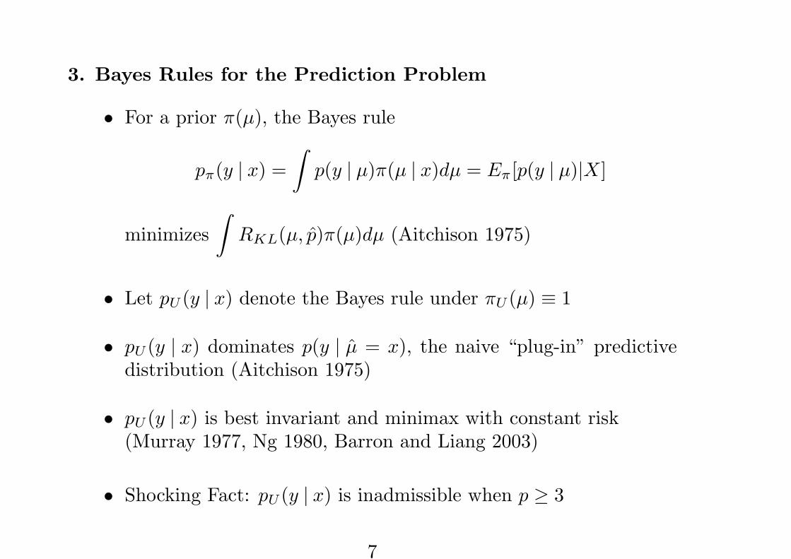
3. Bayes Rules for the Prediction Problem
• For a prior π(µ), the Bayes rule
pπ(y | x) =∫
p(y | µ)π(µ | x)dµ = Eπ[p(y | µ)|X]
minimizes∫
RKL(µ, p)π(µ)dµ (Aitchison 1975)
• Let pU (y | x) denote the Bayes rule under πU (µ) ≡ 1
• pU (y | x) dominates p(y | µ = x), the naive “plug-in” predictivedistribution (Aitchison 1975)
• pU (y | x) is best invariant and minimax with constant risk(Murray 1977, Ng 1980, Barron and Liang 2003)
• Shocking Fact: pU (y | x) is inadmissible when p ≥ 3
7
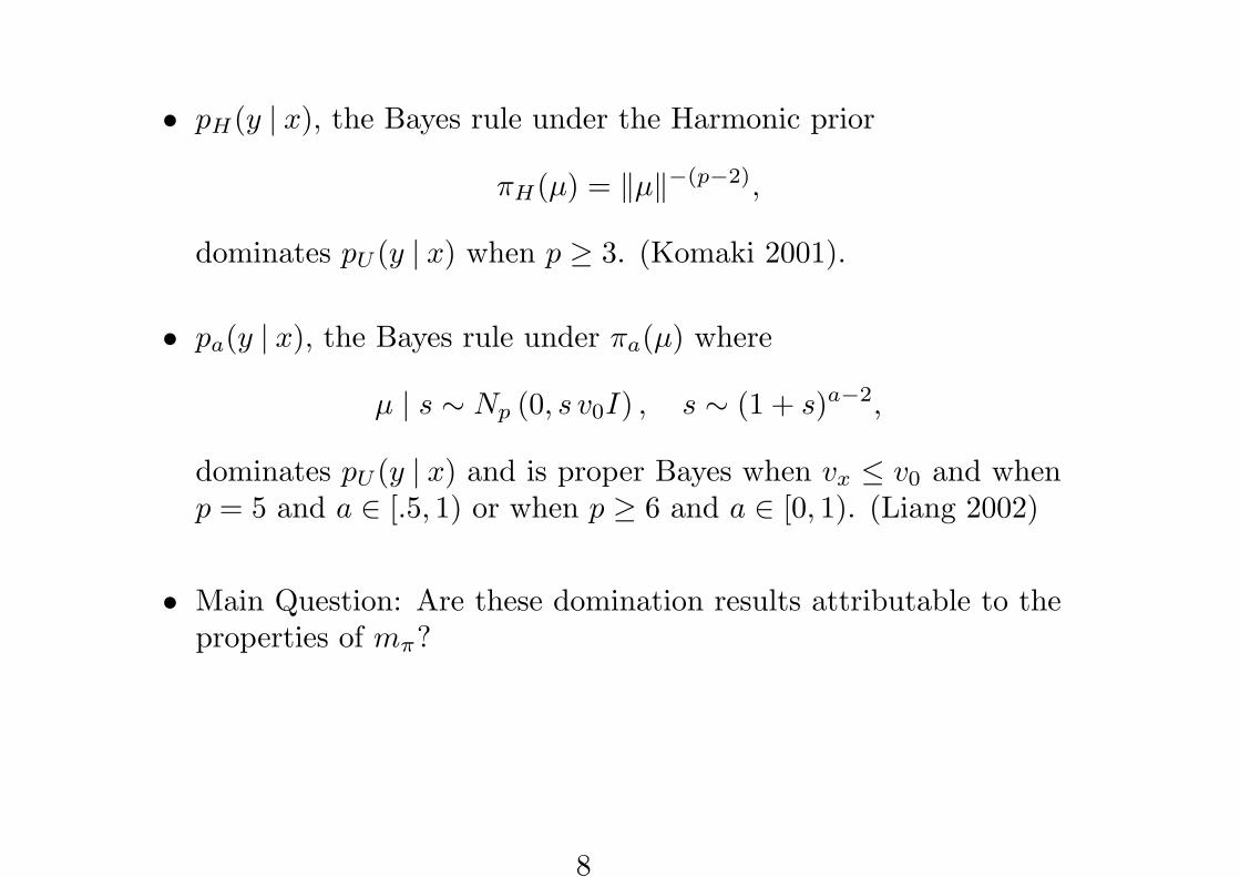
• pH(y | x), the Bayes rule under the Harmonic prior
πH(µ) = ‖µ‖−(p−2),
dominates pU (y | x) when p ≥ 3. (Komaki 2001).
• pa(y | x), the Bayes rule under πa(µ) where
µ | s ∼ Np (0, s v0I) , s ∼ (1 + s)a−2,
dominates pU (y | x) and is proper Bayes when vx ≤ v0 and whenp = 5 and a ∈ [.5, 1) or when p ≥ 6 and a ∈ [0, 1). (Liang 2002)
• Main Question: Are these domination results attributable to theproperties of mπ?
8

4. A Key Representation for pπ(y | x)
• Let mπ(x; vx) denote the marginal of X | µ ∼ Np(µ, vxI) underπ(µ).
• Lemma: The Bayes rule pπ(y | x) can be expressed as
pπ(y | x) =mπ(w; vw)mπ(x; vx)
pU (y | x)
whereW =
vyX + vxY
vx + vy∼ Np(µ, vwI)
• Using this, the risk improvement can be expressed as
RKL(µ, pU )−RKL(µ, pπ) =∫ ∫
pvx(x|µ) pvy (y|µ) logpπ(y | x)pU (y | x)
dxdy
= Eµ,vwlog mπ(W ; vw)−Eµ,vx
log mπ(X; vx)
9
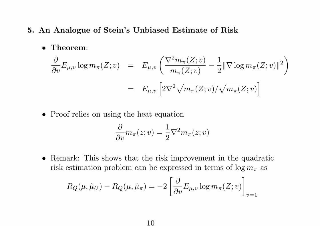
5. An Analogue of Stein’s Unbiased Estimate of Risk
• Theorem:
∂
∂vEµ,v log mπ(Z; v) = Eµ,v
(∇2mπ(Z; v)mπ(Z; v)
− 12‖∇ log mπ(Z; v)‖2
)
= Eµ,v
[2∇2
√mπ(Z; v)/
√mπ(Z; v)
]
• Proof relies on using the heat equation
∂
∂vmπ(z; v) =
12∇2mπ(z; v)
• Remark: This shows that the risk improvement in the quadraticrisk estimation problem can be expressed in terms of log mπ as
RQ(µ, µU )−RQ(µ, µπ) = −2[
∂
∂vEµ,v log mπ(Z; v)
]
v=1
10
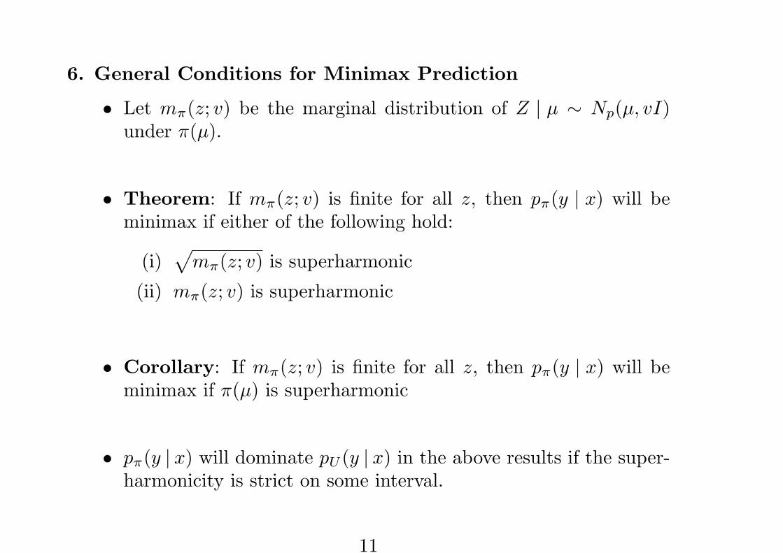
6. General Conditions for Minimax Prediction
• Let mπ(z; v) be the marginal distribution of Z | µ ∼ Np(µ, vI)under π(µ).
• Theorem: If mπ(z; v) is finite for all z, then pπ(y | x) will beminimax if either of the following hold:
(i)√
mπ(z; v) is superharmonic
(ii) mπ(z; v) is superharmonic
• Corollary: If mπ(z; v) is finite for all z, then pπ(y | x) will beminimax if π(µ) is superharmonic
• pπ(y | x) will dominate pU (y | x) in the above results if the super-harmonicity is strict on some interval.
11
7. Sufficient Conditions for Admissibility
• Theorem (Blyth’s Method): If there is a sequence of finite non-negative measures satisfying πn({µ : ‖µ‖ ≤ 1}) ≥ 1 such that
Eπn [RKL(µ, q)]− Eπn [RKL(µ, pπn)] → 0
then q(y | x) is admissible.
• Theorem: For any two Bayes rules pπ and pπn
Eπn [RKL(µ, pπ)]−Eπn [RKL(µ, pπn)] =12
∫ vx
vw
∫ ‖∇hn(z; v)‖2hn(z; v)
mπ(z; v)dzdv
where hn(z; v) = mπn(z; v)/mπ(z; v).
• Using the explicit construction of πn(µ) from Brown and Hwang(1984), we obtain tail behavior conditions that prove admissibilityof pU (y |x) when p ≤ 2, and admissibility of pH(y |x) when p ≥ 3.
12

8. Minimax Shrinkage Towards 0
• Because πH and√
ma are superharmonic under suitable condi-tions, the result that pH(y | x) and pa(y | x) dominate pU (y | x)and are minimax follows immediately from the Theorem.
• By the Theorem, any of the improper superharmonic t-priors ofFaith (1978) or any of the proper generalized t-priors of Four-drinier, Strawderman and Wells (1998) yield Bayes rules thatdominate pU (y | x) and are minimax.
• The risk functions RKL(µ, pH) and RKL(µ, pa) take on their min-ima at µ = 0, and then asymptote up to RKL(µ, pU ) as ‖µ‖ → ∞.
13
• Figure 1a displays the difference between the risk functions
[RKL(µ, pU )−RKL(µ, pH)]
at µ = (c, . . . , c)′, 0 ≤ c ≤ 4 when vx = 1 and vy = 0.2 fordimensions p = 3, 5, 7, 9.
• Figure 1b displays the difference between the risk functions
[RKL(µ, pU )−RKL(µ, pa)]
at µ = (c, . . . , c)′, 0 ≤ c ≤ 4 when a = 0.5, vx = 1 and vy = 0.2for dimensions p = 3, 5, 7, 9.
14
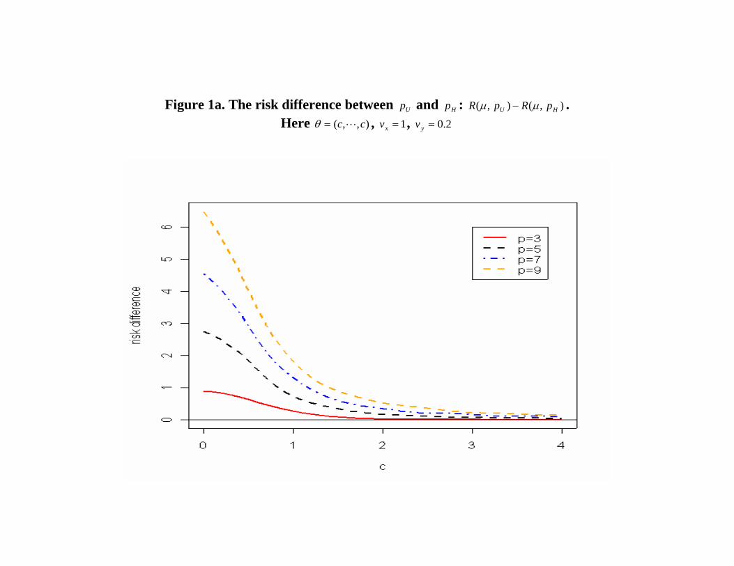
Figure 1a. The risk difference between Up and Hp : ),(),( HU pRpR µµ − .
Here ),,( cc L=θ , 1=xv , 2.0=yv
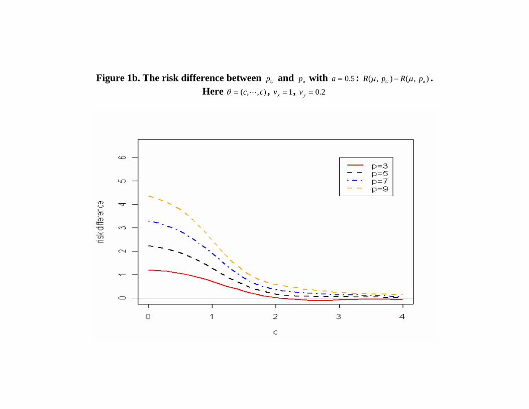
Figure 1b. The risk difference between Up and ap with 5.0=a : ),(),( aU pRpR µµ − .
Here ),,( cc L=θ , 1=xv , 2.0=yv
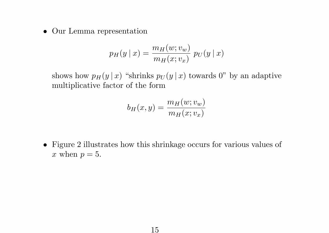
• Our Lemma representation
pH(y | x) =mH(w; vw)mH(x; vx)
pU (y | x)
shows how pH(y | x) “shrinks pU (y | x) towards 0” by an adaptivemultiplicative factor of the form
bH(x, y) =mH(w; vw)mH(x; vx)
• Figure 2 illustrates how this shrinkage occurs for various values ofx when p = 5.
15
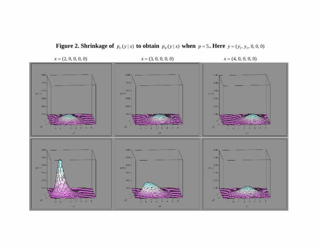
Figure 2. Shrinkage of )|( xypU to obtain )|( xypH when 5=p . Here )0,0,0,,( 21 yyy =
)0,0,0,0,2(=x )0,0,0,0,3(=x )0,0,0,0,4(=x
9. Shrinkage Towards Points or Subspaces
• We can trivially modify the previous priors and predictive distri-butions to shrink towards an arbitrary point b ∈ Rp.
• Consider the recentered prior
πb(µ) = π(µ− b)
and corresponding recentered marginal
mbπ(z; v) = mπ(z − b; v).
• This yields a predictive distribution
pbπ(y | x) =
mbπ(w; vw)
mbπ(x; vx)
pU (y | x)
that now shrinks pU (y | x) towards b rather than 0.
16
• More generally, we can shrink pU (y | x) towards any subspace Bof Rp whenever π, and hence mπ, is spherically symmetric.
• Letting PBz be the projection of z onto B, shrinkage towards Bis obtained by using the recentered prior
πB(µ) = π(µ− PBµ)
which yields the reecentered marginal
mBπ (z; v) := mπ(z − PBz; v).
• This modification yields a predictive distribution
pBπ (y | x) =
mBπ (w; vw)
mBπ (x; vx)
pU (y | x)
that now shrinks pU (y | x) towards B.
• If mBπ (z; v) satisfies any of the conditions of the Theorem, then
pBπ (y | x) will dominate pU (y | x) and be minimax.
17
10. Minimax Multiple Shrinkage Prediction
• For any spherically symmetric prior, a set of subspaces B1, . . . , BN ,and corresponding probabilities w1, ..., wN , consider the recen-tered mixture prior
π∗(µ) =N∑
i=1
wi πBi(µ),
and corresponding recentered mixture marginal
m∗(z; v) =N∑1
wi mBiπ (z; v).
• Applying the µπ(X) = X+∇ log mπ(X) construction with m∗(X; v)yields minimax multiple shrinkage estimators of µ. (George 1986)
18
• Applying the predictive construction with m∗(z; v) yields
p∗(y | x) =N∑
i=1
p(Bi | x) pBiπ (y | x)
where pBiπ (y | x) is a single target predictive distribution and
p(Bi | x) =wim
Biπ (x; vx)∑N
i=1 wimBiπ (x; vx)
is the posterior weight on the ith prior component.
• Theorem: If each mBiπ (z; v) is superharmonic, then p∗(y | x) will
dominate pU (y | x) and will be minimax.
19
• Figure 3 illustrates the risk reduction
[RKL(µ, pU )−RKL(µ, pH∗)]
for µ = (c, . . . , c)′ obtained by pH∗ which adaptively shrinkspU (y | x) towards the closer of the two points b1 = (2, . . . , 2) andb2 = (−2, . . . ,−2) using equal weights w1 = w2 = 0.5
20
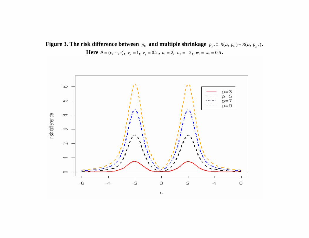
Figure 3. The risk difference between Up and multiple shrinkage *Hp : ),(),( *HU pRpR µµ − .
Here ),,( cc L=θ , 1=xv , 2.0=yv , ,21 =a 22 −=a , 5.021 == ww .
11. The Case of Unknown Variance
• If vx and vy are unknown, suppose there exists an available inde-pendent estimate of vx of the form s/k where
S ∼ vxχ2k.
Also assume that vy = r vx, for a known constant r.
• Substitute the estimates vx = s/k, vy = rs/k and vw = rr+1s/k
for vx, vy and vw respectively.
• The predictor
p∗π(y | x) =mπ(w; vw)mπ(x; vx)
p∗U (y | x)
will still dominate p∗U (y |x) if any of the conditions of the Theoremare satisfied.
• Note however, p∗U (y | x) is no longer best invariant or minimax.
21
12. A Complete Class Theorem
• Theorem: In the KL risk problem, the class of all generalizedBayes procedures is a complete class.
• A (possibly randomized) decision procedure is a probability dis-tribution G(. | x) for each x over the action space, namely the setof all densities g(· | x) : Rp → R of Y . The Bayes rule under aprior π can then be denoted Gπ(. |x) =
∫p(y |µ)pπ(µ |x)dµ, which
is a nonrandomized rule.
• The complete class result is proved by showing;
(i) If G is an admissible procedure, then it is non-randomized.
(ii) There exists a sequence of priors {πi} such that Gπi(. |x) →G(. | x) weak* for a.e. x.
(iii) We can find a subsequence {πi′} of {πi} and a limiting priorπ, which satisfy πi′ → π weak∗ and Gπi′ (. | x) → Gπ(. | x)weak∗ for a.e. x. Therefore, G(. |x) = Gπ(. |x) for a.e. x, sothat G is a generalized Bayes rule.
22
References For Getting Started
Brown, L.D., George, E.I. and Xu, X. (2005). Admissible PredictiveEstimation. Working paper.
George, E.I., Liang, F. and Xu, X. (2005). Improved Minimax Predic-tive Densities under Kullback-Leibler Loss. Annals of Statistics,to appear.
23