markov chain monte carlo sampling for dependency...
TRANSCRIPT
Markov Chain Monte Carlo Sampling forDependency Trees
Von der Fakultat fur Mathematik und Informatik
der Universitat Leipzig
angenommene
DISSERTATION
zur Erlangung des akademischen Grades
DOCTOR RERUM NATURALIUM
(Dr. rer. nat.)
im Fachgebiet
INFORMATIK
vorgelegt
von Christoph Teichmann M.A.
geboren am 26.06.1985 in Friedrichroda
Die Annahme der Dissertation wurde empfohlen von:
1. Professor Dr. Gerhard Heyer (Universitat Leipzig)
2. Professor Dr. Anders Søgaard (Universitat Kopenhagen)
Die Verleihung des akademischen Grades erfolgt mit Bestehen derVerteidigung am 13.05.2014 mit dem Gesamtpradikat
magna cum laude

2

Acknowledgements
Like anyone who has spent a good portion of his or her life on a singletask I am deeply indebted to many people. First and foremost my parents,whose continued and unconditional support has been important throughoutmy life. My brother was always a reliable source of transportation and acalming presence.
No thesis would be the same without the contributions and support of agood advisor. I owe a lot to Gerhard Heyer for taking this role and makingsure that I have the necessary resources both financially and intellectually.
The financing of this thesis was ensured both by participating in theInternational Max Planck School “Neuroscience of Communication” and byworking in the CLARIN-D project. I am grateful for both opportunities.Antje Hollander supported me in the time I spent in the IMPRS and VolkerBohlke was a great colleague during my time in CLARIN-D.
Other colleagues that I am thankful for are Robert Remus, Florian Holz,Ingmar Schuster, Dirk Goldhahn and Amit Kirschenbaum which were avail-able for interesting discussion throughout and were a joy to work with. DirkGoldhahn also provided some help with the formalities surrounding the com-pletion of this thesis.
Whenever I needed a recommendation or other contacts Anders Søgaard,Malte Zimmermann, Thomas Hanneforth and Jonas Kuhn were more thanhelpful.
Daniel Quernheim endured many of my crazy ideas and was graciousenough to humour me when he could have made better use of his time andthe yearly holidays would not have been the same without Stefan Hahnlein.
Finally Antje Bak and Susann Vogel endured my continued breaking ofdeadlines during the final phases of this thesis.
All errors in content, presentation and grammar are my own.It is sometimes expected that a acknowledgement section contains some
form of joke. This one does not.
3

4

Contents
1 Introduction 9
1.1 Overview . . . . . . . . . . . . . . . . . . . . . . . . . . . . . 9
1.1.1 Local MCMC Strategies . . . . . . . . . . . . . . . . . 10
1.1.2 Global MCMC Strategies . . . . . . . . . . . . . . . . 10
1.1.3 Evaluation . . . . . . . . . . . . . . . . . . . . . . . . 11
1.1.4 Contributions . . . . . . . . . . . . . . . . . . . . . . . 11
1.2 Relevance of Dependency Trees . . . . . . . . . . . . . . . . . 12
1.3 Sampling for Dependency Trees . . . . . . . . . . . . . . . . . 14
1.4 Design Goals . . . . . . . . . . . . . . . . . . . . . . . . . . . 16
1.5 Why Markov Chain Monte Carlo? . . . . . . . . . . . . . . . 18
1.6 Outline of the Thesis . . . . . . . . . . . . . . . . . . . . . . . 19
1.7 Programming Libraries and Other Tools Used . . . . . . . . . 20
2 Background 21
2.1 Sampling . . . . . . . . . . . . . . . . . . . . . . . . . . . . . 21
2.1.1 Introduction to Markov Chains . . . . . . . . . . . . . 23
2.1.2 Markov Chain Monte Carlo . . . . . . . . . . . . . . . 29
2.2 Dependency . . . . . . . . . . . . . . . . . . . . . . . . . . . . 31
3 Sampling Dependency Trees with Markov Chain Monte Carlo 37
3.1 Introduction . . . . . . . . . . . . . . . . . . . . . . . . . . . . 37
3.2 State of the Art . . . . . . . . . . . . . . . . . . . . . . . . . . 40
3.3 Basic Algorithms . . . . . . . . . . . . . . . . . . . . . . . . . 46
3.3.1 Ensuring Treeness and Other Constraints . . . . . . . 47
3.3.2 Gibbs and Metropolis-Hastings Samplers . . . . . . . 54
3.3.3 Sampling with the Single Root Constraint . . . . . . . 60
3.3.4 Sampling with the Projective Constraint . . . . . . . . 68
3.4 Sampling with Global Changes . . . . . . . . . . . . . . . . . 77
3.4.1 Sampling from a Factored Distribution . . . . . . . . . 78
3.4.2 Sampling by Greedy Construction . . . . . . . . . . . 86
3.5 Conclusion . . . . . . . . . . . . . . . . . . . . . . . . . . . . 99
5
6 CONTENTS
4 Convergence Evaluation on an Artificial Problem 1014.1 Introduction . . . . . . . . . . . . . . . . . . . . . . . . . . . . 101
4.1.1 A Note on the Development of the Algorithms . . . . 1034.2 The Probability Function . . . . . . . . . . . . . . . . . . . . 1044.3 The Evaluation Parameters . . . . . . . . . . . . . . . . . . . 107
4.3.1 Initialization . . . . . . . . . . . . . . . . . . . . . . . 1084.3.2 Auxiliary Functions . . . . . . . . . . . . . . . . . . . 109
4.4 Algorithms Evaluated . . . . . . . . . . . . . . . . . . . . . . 1104.5 Statistics Used . . . . . . . . . . . . . . . . . . . . . . . . . . 113
4.5.1 Ratio of Reference Assignments . . . . . . . . . . . . . 1134.5.2 The Third Quartile . . . . . . . . . . . . . . . . . . . . 1144.5.3 Count of Reference Assignments . . . . . . . . . . . . 1144.5.4 Function Evaluations . . . . . . . . . . . . . . . . . . . 1154.5.5 Auxiliary Function Evaluations . . . . . . . . . . . . . 115
4.6 Evaluation Results . . . . . . . . . . . . . . . . . . . . . . . . 1154.6.1 Reference Structures with the Same Root - Short Trees1164.6.2 Reference Structures with the Same Root - Medium
Trees . . . . . . . . . . . . . . . . . . . . . . . . . . . . 1324.6.3 Reference Structures with the Same Root - Longer Trees1464.6.4 First Discussion of Results . . . . . . . . . . . . . . . . 1504.6.5 Reference Structures with Differing Roots - Short Trees1514.6.6 Reference Structures with Differing Roots - Medium
Trees . . . . . . . . . . . . . . . . . . . . . . . . . . . . 1524.6.7 Reference Structures with Differing Roots - Long Trees 157
4.7 Conclusions and Future Research . . . . . . . . . . . . . . . . 168
5 Evaluation on an Unsupervised Dependency Parsing Task 1715.1 State of the Art . . . . . . . . . . . . . . . . . . . . . . . . . . 172
5.1.1 Self Alignment Model . . . . . . . . . . . . . . . . . . 1745.2 The Model . . . . . . . . . . . . . . . . . . . . . . . . . . . . 175
5.2.1 Tag to Tag Weight Function . . . . . . . . . . . . . . . 1765.2.2 Distance Weight Function . . . . . . . . . . . . . . . . 1775.2.3 Fertility Weight Function . . . . . . . . . . . . . . . . 178
5.3 Why Sampling is Necessary . . . . . . . . . . . . . . . . . . . 1795.3.1 Why Single Rooted Sampling is Necessary . . . . . . . 179
5.4 Evaluation Setting . . . . . . . . . . . . . . . . . . . . . . . . 1805.4.1 Initialization . . . . . . . . . . . . . . . . . . . . . . . 1805.4.2 Implementation of Sampling and Derivation of a Result1805.4.3 Auxiliary Function . . . . . . . . . . . . . . . . . . . . 1825.4.4 Statistics Used . . . . . . . . . . . . . . . . . . . . . . 182
5.5 Data Used . . . . . . . . . . . . . . . . . . . . . . . . . . . . . 1845.6 Pure Alignment Model . . . . . . . . . . . . . . . . . . . . . . 185
5.6.1 Convergence of the Sampling Process . . . . . . . . . 1865.6.2 Quality of the Generated Parses . . . . . . . . . . . . 194
CONTENTS 7
5.7 Annealing . . . . . . . . . . . . . . . . . . . . . . . . . . . . . 2005.7.1 Convergence of the Sampling Process . . . . . . . . . 2015.7.2 Quality of the Generated Parses . . . . . . . . . . . . 201
5.8 Extending the Model . . . . . . . . . . . . . . . . . . . . . . . 2015.8.1 Convergence of the Sampling Process . . . . . . . . . 2075.8.2 Quality of the Generated Parses . . . . . . . . . . . . 207
5.9 Conclusion and Further Research . . . . . . . . . . . . . . . . 211
6 Conclusion and Further Research 2136.1 Results . . . . . . . . . . . . . . . . . . . . . . . . . . . . . . . 214
6.1.1 The Surprising Helpfulness of Restricted Options . . . 2146.1.2 Usefulness of Global Steps . . . . . . . . . . . . . . . . 2156.1.3 The Surprising Efficiency of Simple Samplers . . . . . 2166.1.4 The Reliability of Gibbs Sampling . . . . . . . . . . . 216
6.2 Further Research . . . . . . . . . . . . . . . . . . . . . . . . . 2176.2.1 Other Unsupervised Dependency Models . . . . . . . . 2176.2.2 Use with Different Tasks . . . . . . . . . . . . . . . . . 2186.2.3 Population Based Techniques . . . . . . . . . . . . . . 218
6.3 Conclusion . . . . . . . . . . . . . . . . . . . . . . . . . . . . 219
7 Bibliography 221
List of Figures 233
List of algorithms 237

8 CONTENTS

Chapter 1
Introduction
1.1 Overview
This section and its subsections give a very general overview of the topics ofthis thesis. In the remainder of this chapter some of these themes are thenelaborated on.
The work concerns itself with the task of sampling dependency trees. De-pendency trees are a formalism for expressing the internal syntactic struc-ture of sentences and they are frequently used in Natural Language Pro-cessing [59]. Sentences which are annotated in this way can serve as aninput for further Natural Language Processing tools solving tasks as diverseas translation, discourse analysis, information retrieval and language mod-elling [59, 42, 43, 16]. In recent years more and more complicated modelsfor the generation of dependency structures have been proposed. They tendto violate the independence assumptions which have traditionally been nec-essary in order to implement fast, exact algorithms for the computation ofall kinds of sums and optima and some workaround must often be found tomake use of these models [83, 59, 82, 84, 72, 74].
In this environment approximate techniques become more and moreinteresting. They often represent a principled way to implement theseworkarounds. One of the most widely used approximation techniques issampling from some distribution of interest [40, 97]. By generating a se-quence of examples distributed according to some probability function ofinterest, it is possible to both produce a guess concerning the position ofoptima and, maybe even more importantly, generate an approximation ofrelevant sums. Often these sums are expectations. These play a central rolein Machine Learning [2, 3, 6, 92].
Markov Chain Monte Carlo Methods (MCMC) [40, 97, 64, 63] are a gen-eral technique for sampling from complex distributions and there have beensome previous attempts at the implementation of MCMC techniques for de-pendency trees. These investigations have come in two flavours. Some have
9

10 CHAPTER 1. INTRODUCTION
basically reduced the problem to the sampling of integer valued vectors, ei-ther by ignoring the internal structure of dependency trees or by attemptingto capture this structure in an ad hoc manner [78, 69]. Others have onlyregarded subsets of the possible dependency trees and have made use of al-ternate representations [67, 70, 68, 115, 8]. The latter algorithms also oftenrequire some auxiliary design choices that have to be made for every newmodel. In this thesis a series of MCMC sampling algorithms is developedthat is both applicable to general dependency trees, while respecting andexploiting their structure, and able to deal with more constraint problems.These constraint settings are the sampling of projective dependency treesand trees that have only a single root word. It will be seen that the firstproblem can be dealt with quite elegantly by extending the main techniquesof the thesis, while the latter requires some additional effort.
1.1.1 Local MCMC Strategies
One of the main results of the thesis are local strategies which change thestructure of dependency trees by little increments and which have the benefitof being simple, out-of-the-box solutions that can be applied to almost anymodel. Because these techniques make only small changes, which are alsoexpected to not violate any of the constraints in any of their intermediatesteps, the question becomes whether they can successfully explore the com-plete space of the admissible trees. The thesis provides theoretical insightand proofs detailing the conditions which must be met in order for this tobe the case. Where the single root constraint makes it impossible to easilyextend the basic techniques, more complicated ones are proposed to handlethis problem without sacrificing generality.
1.1.2 Global MCMC Strategies
Sampling approaches that are based on small local steps can easily become“stuck” in the area around one of the optima of the function to which theyare applied [64]. This problem can be mitigated somewhat by extending thesampling algorithms with steps that change the dependency tree “globally”- techniques that transform the complete tree structure in a single move[56, 115]. For this to be feasible it is necessary to use an auxiliary functionto approximate the actual model which is sampled. This thesis develops suchtechniques and proves their correctness. To the knowledge of the author thisis the first time that such an approach has been proposed for unrestricteddependency trees. Similar techniques have been applied to projective de-pendency trees and constituency trees by other authors[56, 115, 68]. Oneof the global steps developed here is widely applicable for any type of con-straint that may be imposed on dependency trees. This technique is basedon greedily constructing a complete dependency tree. The other global ap-
1.1. OVERVIEW 11
proach, based on sampling spanning trees from weighted graphs, is morerestricted, but can potentially be used with less computational resourcesand with a more easily designed approximation.
1.1.3 Evaluation
While the presentation of the new algorithms in this thesis includes a dis-cussion of their runtime properties and proofs of their correctness, no pre-sentation of a new algorithm is complete without some evaluation of theirperformance on actual tasks. This is done with two different scenarios. Thefirst is an artificial model that allows for diagnosing the convergence of thesampling process towards some analytically predictable expectations. Prob-lems with some actual relevance in Natural Language Processing lack thisfeature - otherwise there would be no reason to apply an approximationtechnique. This allows for some very detailed evaluation.
The second evaluation task is an unsupervised learning task[6, 57]. Anexisting model for the unsupervised prediction of dependency trees [69] isslightly extended and the behaviour of the sampling algorithms is presentedand discussed. It is not possible to use this problem for a detailed evaluationas far as computing expected values goes. Again, if this were otherwise therewould be no reason to use MCMC. This means that the insights gained fromthis evaluation are somewhat weaker than those from the artificial task. Atthe same time the unsupervised learning task is likely to have more relevanceto practitioners which think about using the algorithms.
1.1.4 Contributions
The thesis develops a set of small change algorithms on the basis of wellestablished principles that can be applied to very general models and whichwill usually move to sample at least around one local optimum of that model.These samplers are shown to be correct and remarks on their efficient im-plementation are made. In order to help the exploration of the space of de-pendency trees, even in case of models that generate multiple optima, someglobal sampling techniques are presented that help in escaping these optimain a single, large step. All of the presented algorithms are couched in theMarkov Chain Monte Carlo Framework and could easily be combined withother techniques developed to improve MCMC techniques. Two constraintson dependency tree structures and their handling by sampling algorithmsare discussed. Restricting consideration to projective and/or single rootedtrees is not only an end in itself, a way it might be seen because both areargued to be helpful linguistic constraints, but can also provide some in-spiration how other constraints may be handled. The developed algorithmsare then evaluated extensively on two tasks. One a complicated artificialproblem that allows deep insight into the behaviour of the MCMC schemes
12 CHAPTER 1. INTRODUCTION
and the other a more applied unsupervised learning task. In this evaluationit is shown that reducing the set of trees under consideration by constraintscan actually improve the performance of MCMC algorithms.
So far this section has given a birds eye view of the contents of this thesis.The remainder of this chapter will be concerned with elaborating on someof the themes mentioned so far.
1.2 Dependency Trees and Their Relevance to Nat-ural Languages Processing
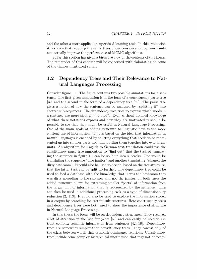
Consider figure 1.1. The figure contains two possible annotations for a sen-tence. The first given annotation is in the form of a constituency parse tree[39] and the second in the form of a dependency tree [59]. The parse treegives a notion of how the sentence can be analysed by “splitting it” intoshorter sub-sequences. The dependency tree tries to express which words ina sentence are more strongly “related”. Even without detailed knowledgeof what these notations express and how they are motivated it should bepossible to see that they might be useful in Natural Language Processing.One of the main goals of adding structure to linguistic data is the moreefficient use of information. This is based on the idea that information innatural languages is encoded by splitting everything that needs to be repre-sented up into smaller parts and then putting them together into ever largerunits. An algorithm for English to German text translation could use theconstituency parse tree annotation to “find out” that the task of translat-ing the sentence in figure 1.1 can be split up into subtasks. One would betranslating the sequence “The janitor” and another translating “cleaned thedirty bathroom”. It could also be used to decide, based on the tree structure,that the latter task can be split up further. The dependency tree could beused to feed a database with the knowledge that it was the bathroom thatwas dirty according to the sentence and not the janitor. In both cases theadded structure allows for extracting smaller “parts” of information fromthe larger unit of information that is represented by the sentence. Thiscan then be used in additional processing task as a type of dimensionalityreduction [2, 113]. It could also be used to explore the information storedin a corpus by searching for certain substructures. Here constituency treesand dependency trees were both used to show the importance of structurein Natural Language Processing.
In this thesis the focus will be on dependency structures. They receiveda lot of attention in the last few years [59] and can easily be used to ex-tract complex semantic information from sentences [42, 16]. Dependencytrees are somewhat simpler than constituency trees. They consist only ofthe edges between words that establish dominance relations. Constituencytrees include some complex hierarchical information that may not be neces-
1.2. RELEVANCE OF DEPENDENCY TREES 13
The janitorcleaned
the dirty bathroom
The janitor cleaned the dirty bathroom ROOT
Figure 1.1: A simple sentence analysed as a parse tree and a dependencytree.
sary in order to extract information from sentences. Dependency structuresalso have the advantage, compared to models that only use linear word ad-jacencies as input [65], that they can represent relationships that are morecomplicated and divided by larger distances. Often certain roles are alsoassigned to the different dependency relations. This is not explored in thisthesis, but the reader should have little trouble in extending the algorithmspresented here to handle labels for the edges.
Dependency edges also express things like argument/predicate relation-ships which are of great importance in natural language grammar [87]. Thisaccounts for the fact that they are such a crucial link between the observedlanguage data and underlying semantic levels.
Dependency trees are seemingly simple structures, but finding the correctdependency tree for a sentence is a non-trivial task [82, 75, 73, 59]. Thismeans that very complex models are generally used to predict dependencytrees.
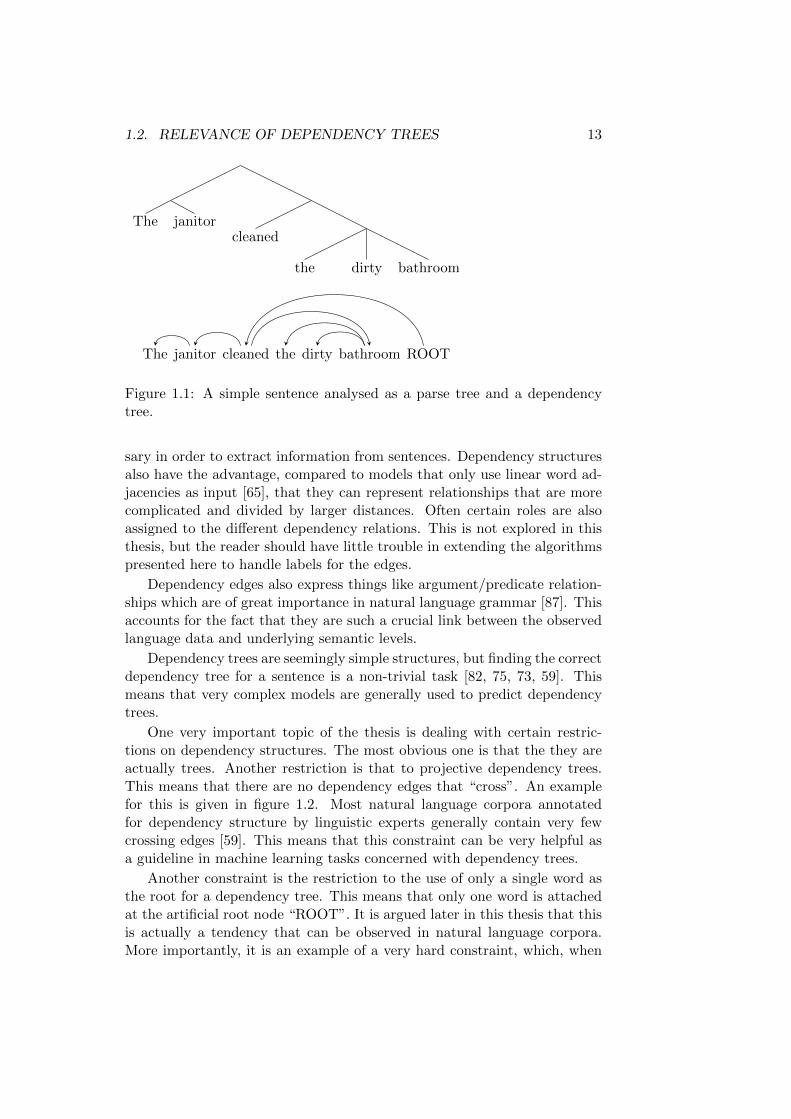
One very important topic of the thesis is dealing with certain restric-tions on dependency structures. The most obvious one is that the they areactually trees. Another restriction is that to projective dependency trees.This means that there are no dependency edges that “cross”. An examplefor this is given in figure 1.2. Most natural language corpora annotatedfor dependency structure by linguistic experts generally contain very fewcrossing edges [59]. This means that this constraint can be very helpful asa guideline in machine learning tasks concerned with dependency trees.
Another constraint is the restriction to the use of only a single word asthe root for a dependency tree. This means that only one word is attachedat the artificial root node “ROOT”. It is argued later in this thesis that thisis actually a tendency that can be observed in natural language corpora.More importantly, it is an example of a very hard constraint, which, when
14 CHAPTER 1. INTRODUCTION
A hearing is scheduled on the issue today ROOT
Figure 1.2: A simple dependency tree with crossing edges. The edge between“hearing” and “on” crosses with that between “scheduled” and “today”.This example is taken from Kubler et. al.[59]
an algorithm can deal with it effectively, can serve as inspiration for howother hard constraints could be handled. A similar hard constraint, thatcould be used instead, would be to force certain words to have exactly oneedge of a specific type. The latter constraint is not considered here since itis very similar in nature to the single root constraint.
1.3 Sampling for Dependency Trees
This thesis develops Markov Chain Monte Carlo (MCMC) algorithms for de-pendency trees. MCMC is generally used for one of two tasks [40]. The firstis approximating a complex sum. The second is stochastic optimization [64].An approximate approach to summation can be necessary when a complexfunction needs to be calculated in order to chose one of a number of possibleoptions. This is important in applications of Bayesian decision theory [2]and Bayesian inference [40, 63]. Summation may also be necessary in otheralgorithms. The widely used expectation maximization algorithm [28, 118]requires that expectations are repeatedly calculated. Since expectations aresums related to a probability function, MCMC algorithms can be extremelyuseful in this context. Expectations are also sometimes necessary to com-pute gradients to train graphical models [3], which have become popular inNatural Language Processing [60, 33, 34, 35, 36, 107, 109]. The describeduse of MCMC to compute sums is the main goal of this thesis and its use inoptimization is a secondary concern.
The use of MCMC in stochastic optimization is related to evolutionaryalgorithms [97] and swarm based optimization [1]. All these algorithmspropose a sequence of possible function arguments in order to find one thatmight maximize or minimize some function of interest. They only differ inthe way these sequences are generated. The advantage that MCMC mayhave compared to the other algorithms is that eventually the frequencywith which arguments are proposed will approach the frequency predictedby the normalized weight function [17]. This means that values with highweight are guaranteed to be visited much more frequently then those with
1.3. SAMPLING FOR DEPENDENCY TREES 15
low probability, at least in the long run. Combining evolutionary algorithmsand MCMC may produce even better optimization techniques [62].
One popular approach for predicting dependency trees is the specifica-tion of some kind of objective function that maps each possible annotationonto a measure of quality. Then the annotation is chosen that maximizesthis measure. This is the most obvious connection between dependency treesand sampling. The actual computation of such a measure of quality mightrequire a complex summation that cannot feasibly be computed analytically.This is often the case if Divide and Conquer approaches can no longer beused because independence assumptions do not apply. This is increasinglybecoming the case for newer dependency models, which use features thatconsider more than a single edge at a time [59]. It is also the case in the un-supervised learning of dependency structures [57, 45] by Bayesian Inference[67, 22], which creates connections between different parses assigned to thesentences in a corpus. In these situations sampling based summation can beused as a technique for approximating an exact value.
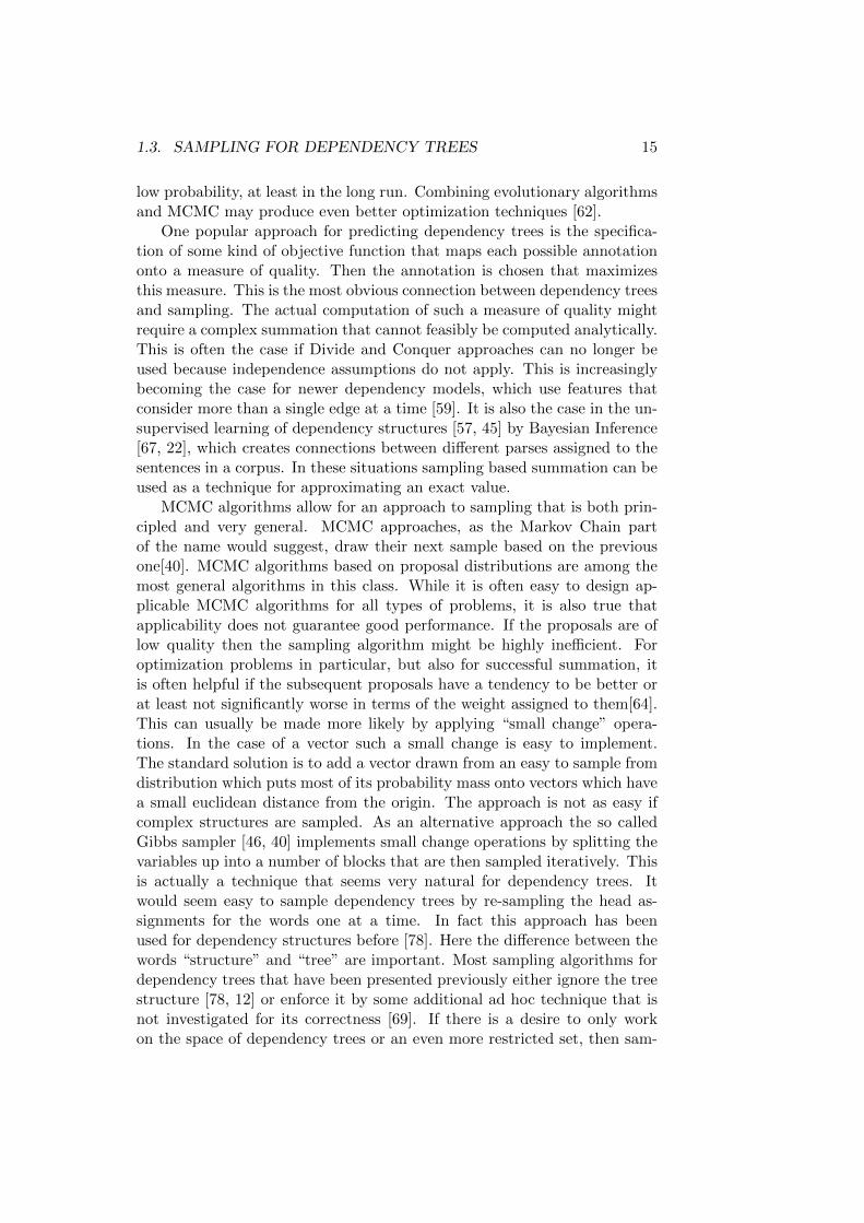
MCMC algorithms allow for an approach to sampling that is both prin-cipled and very general. MCMC approaches, as the Markov Chain partof the name would suggest, draw their next sample based on the previousone[40]. MCMC algorithms based on proposal distributions are among themost general algorithms in this class. While it is often easy to design ap-plicable MCMC algorithms for all types of problems, it is also true thatapplicability does not guarantee good performance. If the proposals are oflow quality then the sampling algorithm might be highly inefficient. Foroptimization problems in particular, but also for successful summation, itis often helpful if the subsequent proposals have a tendency to be better orat least not significantly worse in terms of the weight assigned to them[64].This can usually be made more likely by applying “small change” opera-tions. In the case of a vector such a small change is easy to implement.The standard solution is to add a vector drawn from an easy to sample fromdistribution which puts most of its probability mass onto vectors which havea small euclidean distance from the origin. The approach is not as easy ifcomplex structures are sampled. As an alternative approach the so calledGibbs sampler [46, 40] implements small change operations by splitting thevariables up into a number of blocks that are then sampled iteratively. Thisis actually a technique that seems very natural for dependency trees. Itwould seem easy to sample dependency trees by re-sampling the head as-signments for the words one at a time. In fact this approach has beenused for dependency structures before [78]. Here the difference between thewords “structure” and “tree” are important. Most sampling algorithms fordependency trees that have been presented previously either ignore the treestructure [78, 12] or enforce it by some additional ad hoc technique that isnot investigated for its correctness [69]. If there is a desire to only workon the space of dependency trees or an even more restricted set, then sam-
16 CHAPTER 1. INTRODUCTION
The janitor cleaned the dirty bathroom ROOT
The janitor cleaned the dirty bathroom ROOT
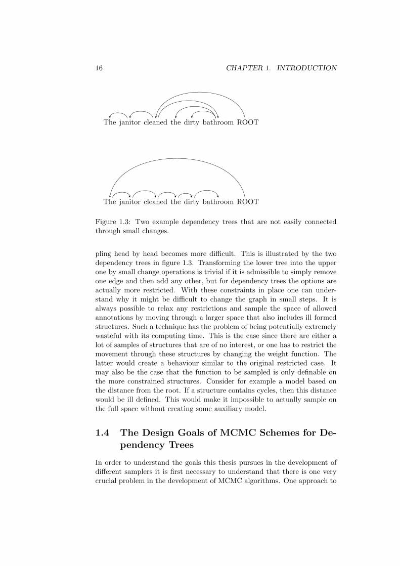
Figure 1.3: Two example dependency trees that are not easily connectedthrough small changes.
pling head by head becomes more difficult. This is illustrated by the twodependency trees in figure 1.3. Transforming the lower tree into the upperone by small change operations is trivial if it is admissible to simply removeone edge and then add any other, but for dependency trees the options areactually more restricted. With these constraints in place one can under-stand why it might be difficult to change the graph in small steps. It isalways possible to relax any restrictions and sample the space of allowedannotations by moving through a larger space that also includes ill formedstructures. Such a technique has the problem of being potentially extremelywasteful with its computing time. This is the case since there are either alot of samples of structures that are of no interest, or one has to restrict themovement through these structures by changing the weight function. Thelatter would create a behaviour similar to the original restricted case. Itmay also be the case that the function to be sampled is only definable onthe more constrained structures. Consider for example a model based onthe distance from the root. If a structure contains cycles, then this distancewould be ill defined. This would make it impossible to actually sample onthe full space without creating some auxiliary model.
1.4 The Design Goals of MCMC Schemes for De-pendency Trees
In order to understand the goals this thesis pursues in the development ofdifferent samplers it is first necessary to understand that there is one verycrucial problem in the development of MCMC algorithms. One approach to

1.4. DESIGN GOALS 17
MCMC that will be used throughout this thesis is based on the Metropolis-Hastings style of MCMC sampling. This means that given the last samplethat was created a new value is drawn from some proposal density and thenaccepted or rejected. Here acceptance means that the new value is usedas the next sample, while rejection means that the last values is repeated.Acceptance is generally based on the probability value of the new value underthe distribution that one is attempting to sample from. If new proposals areof low probability compared to the preceding value, then they are likely tobe rejected. In summation this can mean that one is “stuck” in a sub-area ofthe space being sampled and this can diminish the quality of the sample. Inoptimization this means that a number of proposals are made that provideno benefit toward searching for an argument with a better function value.In order to avoid an overly large number of rejections, it is generally usefulto propose a new value by making a small change to the last sample thatwas drawn in a style similar to Gibbs sampling as mentioned before [40].This will be one of the guiding principles in developing MCMC samplersthroughout this work. A Gibbs sampler only changes a small number ofvariables at a time and computes an exact probability of this change foreach setting of the variables. In this thesis, these variables will be thesingle heads. MCMC algorithms are developed throughout that sample thedependency trees one head at a time. One strain will be considered witha Gibbs style sampler that thoroughly explores the possible settings whileanother will sample head by head with uniformly random proposals whichsave a large number of computations. It will be seen that, at least as faras reaching a local optimum goes, both algorithms are surprisingly efficient.Being able to reach such an optimum quickly is important in sampling sincethese need to be represented with high frequency in any sample. At the sametime this head by head change can lead to making “steps” that are too smallor iterating inside a small subsection of the sampling space. Both problemscan usually be characterized as being “stuck” in local optima. Once a valuehas been found that has a high probability samples similar to it will begenerated over and over again. This is complicated even further by the factthat structured variables are sampled. The dependency trees are bound bytheir tree property. Then there are also the constraints to projective treesand single roots that are investigated here. These make it even harder tomove freely through the space of possible settings. For optimization thismeans an insufficient exploration of the space of possible annotations. Forsummation it means that the convergence towards the desired expectationscan take a long time. In order to solve this problem the sampling in smallsteps will be extended by a number of approaches that allow for makinglarger, global steps. These strategies will be general enough to allow fortheir extension to a number of similar problems.
Now the twin goals of being able to sample by making small changes andbeing able to escape local optima by enabling informed proposals on a more
18 CHAPTER 1. INTRODUCTION
global level are in place. The last goal that will be pursued through thethesis is that of generality. The samplers that are developed should workwith a wide range of measures of quality or functions to be summed. Partof this goal is also to keep the number of parameters that need to be tunedsmall. This could encourage an out of the box use of the samplers by prac-titioners and allow for more time being spend on searching for interestingmodels instead of developing algorithms to work with them. This goal issomewhat weakened in order to allow for global steps, which will require aform of auxiliary weight functions. Since MCMC schemes can be combinedsurprisingly easily, the global schemes will generally be combined with thelocal approaches. This means an attempt is made to make a single large,global step and then “fine tune” the settings with the more local approaches.
1.5 Why Markov Chain Monte Carlo?
Sampling based approaches are used when there is no obvious way of solvingthe problem of summing or optimizing some given goal function exactly.Both tasks can still be computationally expensive and often there are noguarantees of finding a good solution within a given running time. With thisin mind one may question the decision of using sampling based algorithms atall. This question becomes even more obvious when alternatives are broughtinto play. For summation there are approaches like Variational Inferenceand Belief Propagation [6, 3]. For Optimization there are EvolutionaryAlgorithms and the widely used numerical algorithms based on gradients[97, 44].
One of the most obvious benefits of the sampling based approaches isthe fact that they have guarantees with respect to their exactness. Usuallyonly very weak guarantees can be made. These state that a reasonably closeapproximation to an optimum or the distribution in question can be madeeventually. There is also a guarantee that any level of exactness in thesegoals can be achieved. This is usually not offered by variational methodsor Belief Propagation. Gradient based and variational techniques may alsorequire additional information like gradients and expectations. Here thedifferent algorithms can be used together with MCMC, which can providethe expectations needed. Afterwards Variational Inference or gradient basedmethods can be used to solve other parts of the problems in question.
The most well known competitors in the field of optimization that alsohave a similar generality are evolutionary and swarm based algorithms [116,1]. There is little competition here, as it is easy to combine MCMC algo-rithms and Evolutionary Algorithms [30, 62].
Sequential Monte Carlo (SMC) [14, 76] is another sampling based tech-nique and can be used as a direct alternative to MCMC. A derivative of thesemethods is the so called Population Monte Carlo [15]. Both sum up func-
1.6. OUTLINE OF THE THESIS 19
tions by Sampling-Important-Re-Sampling in which a large number of pos-sible new candidates are drawn from a proposal function and then acceptedor rejected based on their relative weight. The reader will immediately seethe similarity to the Metropolis-Hastings method mentioned earlier. Thismeans that1 the algorithms presented here could easily be changed in orderto be usable in this new context.
Almost all commonly used alternatives discussed in this section can makesome use of the results of MCMC techniques. Therefore the work in thisthesis should be seen less as an advocacy for an exclusive use of MCMC andmore as contributing a number of MCMC techniques that may be used ontheir own or in concert with other techniques. The main advantages that willresult from having these techniques are very general solutions to summationproblems. The techniques do not require an overly deep knowledge of theprobability distributions or other functions with which one is trying to work.It is then possible to use these samplers to support other techniques if thisis desired. While this may not lead to techniques that can compete withwell tuned algorithms for specific problems [26], it can save a large amountof time in the development of machine learning techniques and open theway for working with distributions that would have been hard to handleotherwise.
1.6 Outline of the Thesis
The first step that needs to be taken in a thesis is establishing the back-ground information needed. This will be done in chapter 2. In this chaptersampling and Markov Chain Monte Carlo methods are introduced. Depen-dency Trees will also be discussed and presented more thoroughly.
Once this setting of the background is out of the way, chapter 3 intro-duces the algorithms that constitute the main contribution of this thesis.Both the local and global sampling approaches are given. The samplingof dependency structures is only an interesting problem separate from gen-eral MCMC problems because of the constraints they require. Thereforethis chapter also discusses how the restrictions to projective and/or singlerooted trees can be enforced in sampling. It will actually be found that theserestrictions help in sampling by focusing it on a smaller set of possibilities.
Once it has been outlined how the different sampling algorithms work,it is then necessary to evaluate their strengths and weaknesses. This is doneextensively in chapters 4 and 5. In the first an artificial problem is used whichcan be solved analytically and allows a detailed evaluation. The drawbackis the fact that this evaluation is not strongly tied to any applied task. Thisis remedied somewhat in chapter 5 in which an unsupervised parsing modelis used to evaluate the sampling algorithms. It is not possible to solve this
1Especially were Population Monte Carlo is used.

20 CHAPTER 1. INTRODUCTION
problem analytically, resulting in an auxiliary measure of quality being usedused. This makes the evaluation a little less informative.
Throughout the thesis the following results are the core contributions.The simple head by head approaches, which need almost no additional de-sign, are widely applicable and can deal with all types of structural restric-tions in a surprisingly elegant way. In order to move between optima itmay be necessary to use more global steps, requiring some additional designchoices. Finally all these algorithms elaborate on the sparse prior research onMCMC for dependency trees by providing techniques that are both generaland provably correct in the limit.
1.7 Programming Libraries and Other Tools Used
It is necessary to give proper attribution for all the tools used in the gener-ation of this thesis and the data that is used for it.
The code that was used for all evaluation presented here can be found inthe Google Code repository code.google.com/p/gragra/. For the task ofrandom number generation the Colt Library for scientific computation wasused acs.lbl.gov/software/colt/. For some data processing tasks theGuava Tools proved helpful code.google.com/p/guava-libraries/ andall computation was speed up by using the fastutils library fastutil.di.
unimi.it/. The graphs were generated either with the Veusz home.gna.
org/veusz/ or the Graphviz www.graphviz.org/ tool. Both were used intheir Xubuntu versions. The thesis itself was generated using Texmakerwww.xm1math.net/texmaker/ also under Xubuntu.

Chapter 2
Background
This chapter introduces the background material that will be used through-out the thesis as well as notations and some theorems. There is also someadditional background material and discussion of the state of the art in thefollowing chapters. The information given in the other chapters is morespecific to them.
The presentation starts with a discussion of sampling techniques. Thisleads into an outline of Markov Chain Monte Carlo methods used throughoutthe thesis. The structures on which the algorithms operate, dependencytrees, are more clearly defined to close out the chapter. Before all of this isdone some small notational details should be fixed.
The function 1(b) is used to denoted one if b equals true and zero if bequals false. When sequences of elements are written they should usually besurrounded by angular brackets in the form 〈1, 2, . . . , n〉, but the bracketsare dropped whenever this does not reduce clarity. Expressions like x ∈〈x1, x2, . . . , xn〉 are used as a shorthand for x ∈ {y|∃i : xi = y}.
2.1 Sampling
The Markov Chain Monte Carlo techniques discussed here are used for sam-pling. Let P be some function that assigns positive real weights to theelements of some set S. Since this thesis is concerned with structures as-signed to sentences it will generally not be necessary to deal with topics suchas measure theory and it is possible to assume that S is a countable set. Anew, normalized function can be defined by:
P ′(x) =P (x)
Z(2.1)
Z =∑y∈S
P (y) (2.2)
21
22 CHAPTER 2. BACKGROUND
The task of sampling can be defined as generating a sequence of elementsfrom S such that the relative frequency of any element x in the sequence is asclose as possible to P ′(x). This may be important for two reasons. It can beused for a kind of stochastic optimization [97, 17]. That is the case since theelements with high weight should be more frequent in the sampled sequence.It is also possible to compute an approximation of the normalization factorZ and to estimate expectations with respect to P ′ by using the frequenciesin the sample in place of actual probabilities. Because of this sampling canbe seen as a general method for summing complex functions when there isno way of computing such a sum analytically [40, 64]. Obviously any finitesequence can only be an approximation for a function defined on an infiniteset. It is also impossible to exactly approximate a function of arbitraryprecision with a finite sample, but usually only limited precision is needed.
Computing expectations is an important task for Natural LanguageProcessing. Some of the most important instances of sums which are of-ten needed in Natural Language Processing are expectations in probabilis-tic models. They are needed in order to run the popular EM algorithm[28, 118, 81]. If a model is sufficiently complex, then the task of comput-ing expectations can become very hard [89, 107] and an approximation isnecessary. Graphical models, which are often used in Natural LanguagesProcessing, become to complicated for analytical methods when the graphscontain cycles [3, 34, 79]. For this latter task there are actually a numberof approximation algorithms that can be used. An example would be Be-lief Propagation[3, 91]. Even when optimization techniques like stochasticgradient descent are used [97, 35], sampling can be helpful for some mod-els, for example the popular Conditional Random Fields [60, 114], whichrequire the computation of expectations to derive the gradient. Samplingtechniques can be used here as well.
Recently Bayesian Inference [63] has become popular in Natural Lan-guage Processing [8, 18, 19, 29, 49]. In this framework probabilities fordifferent models are defined and some output is chosen which is the mostlikely according to all models weighted by their probability. If it is possible togenerate a sequence that is distributed according to such a complex model,then one could simply select the most frequent outcome in the generatedsequence.
Note that, as is true for almost all types of algorithms, there are anumber of alternative approaches that can be used to replace sampling. Oneexample would be Variational Inference [6], which has gained popularityin Natural Language Processing recently [80, 58, 21, 22]. The techniqueis based on reducing a distance between an approximate model and thedesired distribution. This means that Variational Inference transforms theproblem into an optimization task. It is often more efficient than samplingbut also bounded by the approximate model, while sampling can usuallybe extended to become arbitrarily correct by simply drawing more samples.
2.1. SAMPLING 23
Variational Inference also requires a good understanding of the function thatis approximated. First it is necessary to design a suitable approximationmodel and then steps that reduce the distance have to be computed. Incontrast there are quite a few sampling techniques that only require theability of evaluating the function to be sampled at any point up to somefactor.
The most popular technique for sampling is stochastic simulation[40].Some random process is simulated by using a random number generatorand the sequence of elements generated by it is used as the sample. Forsome simple models it is possible to define such a process so that the subse-quent elements are independent and then just draw them one by one. But ifthe functions of interest become sufficiently complex, then it is nearly impos-sible to generate a sample that accurately approximates the target functionby independent proposals. The well known method of rejection sampling[40] can generate a sequence of samples by proposing values and then eitheradding them to the sample or rejecting them. For a complex function it ishard to propose good candidates and there will be a large number of rejec-tions. In this case it is possible to generate a sequence by using informationfrom elements seen before. This is done in order to improve the propos-als. It also makes it possible to drop normalization factors, which may bevery hard to compute. One probabilistic process used this way are MarkovChains. They are introduced in the next section.
2.1.1 Introduction to Markov Chains
This section is based in large parts on the introduction to Markov Chainsby Norris [85], but it makes a number of simplifications. The main interestof this thesis are finite sets of structures, i.e. corpora, that are assigned afinite number of annotations. This means that it will be sufficient to discussMarkov Chains that have a finite number of states. Making use of hiddenreal parameters would require an extension of the framework. The readerinterested in a more thorough treatment of Markov Chains is referred to thebook by Norris [85]. A number of theorems merely cited here are provenand expanded upon in that work. The natural starting point is defining thegeneral concept of a Markov Chain.
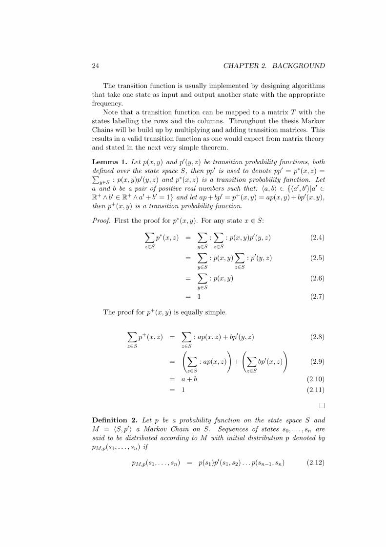
Definition 1 (Markov Chain). Let S be some finite set called the statespace, let p : (S × S) → (0, 1) be a transition probability function fulfillingthe condition:
∀s ∈ S :
(∑s′∈S
p(s, s′)
)= 1.0 (2.3)
then the pair 〈S, p〉 is called a Markov Chain.
24 CHAPTER 2. BACKGROUND
The transition function is usually implemented by designing algorithmsthat take one state as input and output another state with the appropriatefrequency.
Note that a transition function can be mapped to a matrix T with thestates labelling the rows and the columns. Throughout the thesis MarkovChains will be build up by multiplying and adding transition matrices. Thisresults in a valid transition function as one would expect from matrix theoryand stated in the next very simple theorem.
Lemma 1. Let p(x, y) and p′(y, z) be transition probability functions, bothdefined over the state space S, then pp′ is used to denote pp′ = p∗(x, z) =∑
y∈S : p(x, y)p′(y, z) and p∗(x, z) is a transition probability function. Leta and b be a pair of positive real numbers such that: 〈a, b〉 ∈ {〈a′, b′〉|a′ ∈R+ ∧ b′ ∈ R+ ∧ a′+ b′ = 1} and let ap+ bp′ = p+(x, y) = ap(x, y) + bp′(x, y),then p+(x, y) is a transition probability function.
Proof. First the proof for p∗(x, y). For any state x ∈ S:∑z∈S
p∗(x, z) =∑y∈S
:∑z∈S
: p(x, y)p′(y, z) (2.4)
=∑y∈S
: p(x, y)∑z∈S
: p′(y, z) (2.5)
=∑y∈S
: p(x, y) (2.6)
= 1 (2.7)
The proof for p+(x, y) is equally simple.
∑z∈S
p+(x, z) =∑z∈S
: ap(x, z) + bp′(y, z) (2.8)
=
(∑z∈S
: ap(x, z)
)+
(∑z∈S
bp′(x, z)
)(2.9)
= a+ b (2.10)
= 1 (2.11)
Definition 2. Let p be a probability function on the state space S andM = 〈S, p′〉 a Markov Chain on S. Sequences of states s0, . . . , sn aresaid to be distributed according to M with initial distribution p denoted bypM,p(s1, . . . , sn) if
pM,p(s1, . . . , sn) = p(s1)p′(s1, s2) . . . p(sn−1, sn) (2.12)
2.1. SAMPLING 25
The distribution according to an initial function and a Markov chain isthe main concept exploited in this thesis. Usually the initial distributionis given by an algorithm that initializes whatever structures form the stateand then, as stated before, some algorithm is repeatedly applied in order togenerate the necessary sequence. If the algorithm that generates the nextstate is chosen to match up with the transition function, then it is possible togenerate sequences that are distributed according to pM,p(s1, . . . , sn). Thesesequences are the desired samples as long as some properties hold for thetransition function. It is necessary to extend the basic transition probabilityfunction in order to define these properties.
Definition 3 (N-Step Transition Probability Function). Let 〈S, p〉 be aMarkov Chain. Let n ∈ N, 0 < n, then the n-step transtion probabilityfunction is denoted by pn : S × S → (0, 1) and is defined by:
p1(x, y) = p(x, y) (2.13)
pn(x, y) =∑z∈S
: pn−1(x, z)p(z, y) (2.14)
Note that pn is again a valid transition function i.e.:
∀s ∈ S :
(∑s′∈S
pn(s, s′)
)= 1.0 (2.15)
The first requirement for generating proper sample sequences is for themovements of the chain to eventually explore the complete space of possiblestates. The next definition formalizes this.
Definition 4 (Irreducible Markov Chain). Let M = 〈S, p〉 be a MarkovChain. M is called irreducible when there is some n ∈ N, n > 0 such thatpn(x, y) > 0 for any pair 〈x, y〉 in S × S.
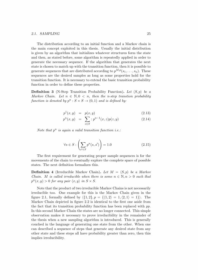
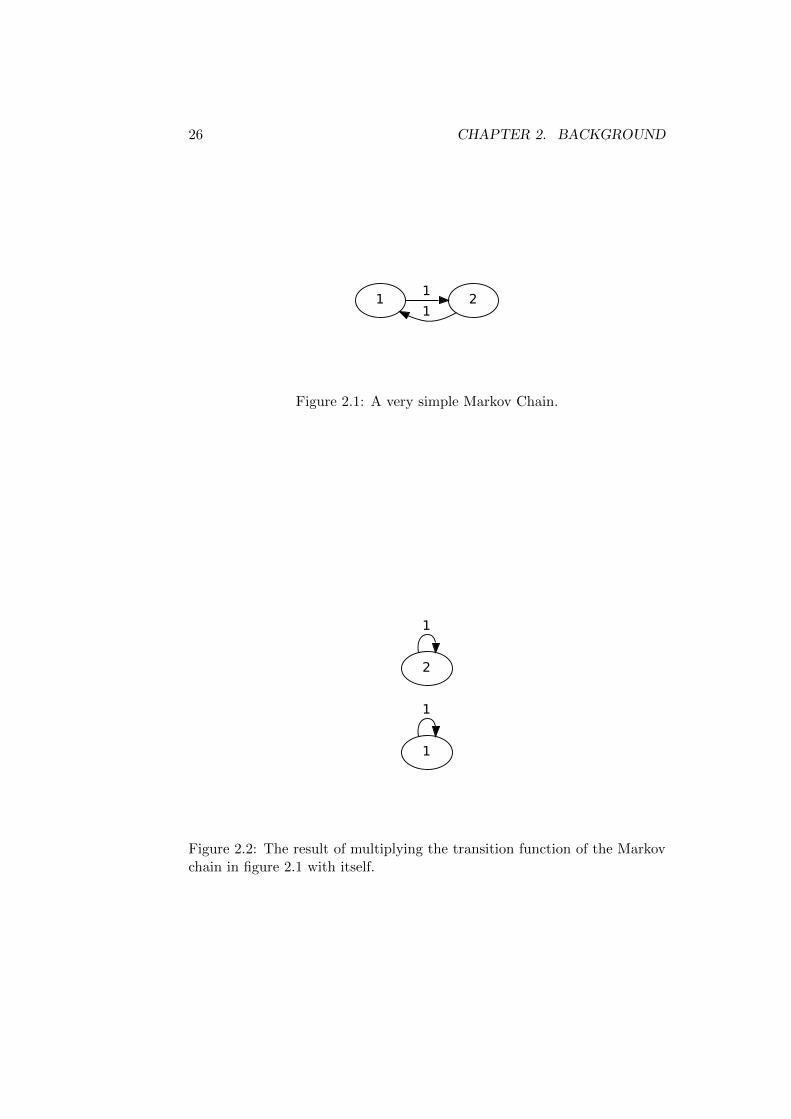
Note that the product of two irreducible Markov Chains is not necessarilyirreducible too. One example for this is the Markov Chain given in thefigure 2.1, formally defined by 〈{1, 2}, p = {〈1, 2〉 = 1, 〈2, 1〉 = 1}〉. TheMarkov Chain depicted in figure 2.2 is identical to the first one aside fromthe fact that its transition probability function has been replaced with pp.In this second Markov Chain the states are no longer connected. This simpleobservation makes it necessary to prove irreducibility in the remainder ofthe thesis when a new sampling algorithm is introduced. This is generallycouched in the language of generating one state from the other. When onecan described a sequence of steps that generate any desired state from anyother state and these steps all have probability greater than zero, then thisimplies irreducibility.
26 CHAPTER 2. BACKGROUND
1 21
1
Figure 2.1: A very simple Markov Chain.
1
1
2
1
Figure 2.2: The result of multiplying the transition function of the Markovchain in figure 2.1 with itself.
2.1. SAMPLING 27
Now would normally be the time to introduce the concept of positiverecurrence. This concept expresses that the expected time taken to returnto any previously visited state is less than infinity. But this is true for everyfinite, irreducible Markov Chain so the concept is ignored here. One finalrequirement that a chain may fulfil in order to allow for correct sampling,but which is not generally necessary, is that of aperiodicity.
Definition 5 (Aperiodicity). A Markov Chain 〈S, p〉 is said to be aperiodicif, for every state s ∈ S, there is some natural number n such that it is truethat pm(s, s) > 0 for every number m ∈ N, n ≤ m.
Note that in the definition the states take scope over the number n.In this thesis aperiodicity is proven by showing that chains can move
in place. This means that the algorithm used to implement the transitionfunction can return the exact state it has been given as input. Given ir-reducibility the aperiodicity follows since there must be some probabilitygreater zero of moving to another state and back and also some probabilityto do arbitrarily many in place steps beforehand. In the special case of asingle state, the property is trivially true.
The next necessary concept is that of a stationary distribution. If thealgorithms implementing the transition function were to be called infinitelywith input states chosen proportionally to a stationary distribution, thenthe return values would have frequencies according to the same distribution.It may not be intuitively clear why this concept is relevant, but there areimportant theorems stating that the behaviour of certain Markov Chains isguided by an invariant distribution.
Definition 6 (Stationary Distribution). Let 〈S, p〉 be a Markov Chain andand let r : S → (0, 1) be a function with the restriction that
∑s∈S : r(s) = 1.
Define rp = {〈y〉 = v|y ∈ S ∧ v =∑
x∈S : r(x)p(x, y)}. If rp = r, then r iscalled a stationary distribution for 〈S, p〉.
It is a useful fact that creating a new chain by taking the product oftwo chains with the same stationary distribution preserves the stationarydistribution.
Lemma 2. If r is a stationary distribution for the Markov Chains 〈S, p〉and 〈S, p′〉, then r is also a stationary distribution for 〈S, pp′〉.Proof.
rpp′(x) =∑s∈S
∑s′∈S
r(s)p(s, s′)p′(s′, x) (2.16)
=∑s′∈S
p(s′, x)∑s∈S
r(s)p(s, s′) (2.17)
=∑s′∈S
r(s′)p(s′, x) (2.18)
= r(x) (2.19)
28 CHAPTER 2. BACKGROUND
This can of course be applied arbitrarily often, always creating newMarkov Chains that preserve stationary distributions. For all chains pre-sented in this thesis it is true that they have only a single stationary distri-bution.
Theorem 1. Let M = 〈S, p〉 be a Markov Chain that is irreducible and forwhich S is finite. Then there is at most one invariant distribution for M .
Proof. This statement follows from theorem 1.7.6 in Norris [85].
The simplest Markov Chain Monte Carlo method is based on repeatedlygenerating a sequence from a Markov Chain and using the last state in thesequence as part of the sample. While this technique is not used here, allalgorithms presented could also be used in this way. The correctness followsfrom the next theorem.
Theorem 2. Let M = 〈S, p〉 be a Markov Chain that is irreducible and forwhich S is finite. If M has invariant distribution r, then ∀i, j ∈ S × S :pn(i, j)→ r(j) as n→∞.
Proof. Follows from theorem 1.8.3 in Norris [85].
The technique that is used is based on the fact that a sequence generatedfrom a Markov Chain will contain elements proportional to the invariantdistribution if the sequence is sufficiently long. This leads to the followingsampling algorithm: start at any state and generate a new state until somepredetermined stopping time. The sequence is then the desired sample. Theprevious theorem was presented as justification to do a number of “burnin” steps used to pick the initial state. It is also possible to ignore someintermediate steps thanks to the preservation of the invariant distributionunder multiplication of the transition function with itself.
The final theorem is:
Theorem 3. Let M = 〈S, p〉 be a Markov Chain that is irreducible and forwhich S is finite. Assume this chain has invariant distribution r and lets1, s2, . . . , sn be a sequence of states with arbitrary initial state S1 generatedfrom M . Then, almost surely, the average number of times any state ispresent in the sequence converges towards its probability according to r asthe length of the sequence approaches infinity.
Proof. Follows from theorems 1.7.7 and 1.10.2 in Norris [85].
This theorem only gives a weak guarantee that the sampling processbehaves correctly. In order to give any information about the number ofsteps necessary to achieve a certain quality of approximation, it would be
2.1. SAMPLING 29
necessary to compute intractable features of the chain. This means that itis important to design the transition function well to hopefully speed upconvergence. Finding out how well certain chains converge is one of themain topics of this thesis.
One main problem of Markov Chain Monte Carlo research is finding waysof constructing a chain to ensure a certain invariant distribution. Generaltechniques used for this purpose are presented in the next section.
2.1.2 Markov Chain Monte Carlo
The last section already outlined how samples can be generated by running aMarkov Chain for some time and then either using the last state as one sam-ple point or the complete sequence as a sample. The main problem is thento design chains having an invariant distribution equal to the probability:
P ′(x) =P (x)
Z(2.20)
where P is the function of interest.
It is generally required to do this without having to compute the nor-malization constant Z. Finding Z is generally intractable. If it is necessaryto compute this value, then the whole point of sampling approaches wouldbe defeated.
It is also very important that the current state can be used very wellin generating the next one. If it is possible to sample efficiently by alwaysmaking independent proposals, then there would be little reason to use theMCMC approach. Instead one could use some technique like importancesampling [63]. The Markov Chain structure makes it possible to use theprevious state in order to create the next one and once a state of high weightaccording to P ′ has been reached, its vicinity can be explored in order togenerate a good sample. Note that a state with high weight according toP ′ should be present frequently in any sample and therefore this movementclose to good previous states is desirable.
Moving between different optima of the function P is another necessityin order to create a sample that actually represents the desired function well.This may be hindered by too local moves of the Markov Chain. All thesethings need to be considered in the creation of chains later in this thesis.This section is primarily concerned with general principles which can beused to design Markov Chains with the correct invariant distributions.
The first technique is based on the concept of detailed balance.
Definition 7 (Detailed Balance). Let M = 〈S, p〉 be a Markov Chain andlet P : S → R+ be a function with:
30 CHAPTER 2. BACKGROUND
∑s∈S
P (s) = 1 (2.21)
then M is said to be in detailed balance with respect to P if it is true forany pair of states i, j from S that:
P (i)p(i, j) = P (j)p(j, i) (2.22)
When a chain is in detailed balance with respect to a distribution P thenthis implies that P is an invariant distribution:
Pp(s′) =∑s∈S
P (s)p(s, s′) (2.23)
=∑s∈S
P (s′)p(s′, s) (2.24)
= P (s′)∑s∈S
p(s′, s) (2.25)
= P (s′) (2.26)
Because detailed balance can be used to ensure any desired invariantdistribution, it is often used in the design of MCMC schemes. By makinguse of the Metropolis-Hastings rule [40, 64, 63] detailed balance is easilyensured. The rule is based on using a proposal function that generates apossible next state. This function can take into consideration the currentstate and therefore qs will denote the proposal function for the state s. Oncea new state s′ has been proposed an accept/reject ratio is computed thatensures detailed balance. Then a random number is generated uniformly inthe interval (0, 1). If the number is greater than the ratio, then the old stateis simply returned as the next step in the sequence, a role otherwise takenby the proposal. This accept/reject ratio is defined by:
min
(1,qs′(s)P
′(s′)
qs(s′)P ′(s)
)(2.27)
Proving that this does indeed ensure detailed balance is left to the reader,who may also find more information on the algorithm by consulting any ofthe typical references such as the book by Gamerman and Lopez [40]. Notethat the ratio increases as the new state becomes more likely. It is thereforedesirable to propose the next state in the sequence by making some slightmodification to the old state so that the value of P ′ does not change tomuch. When sampling is done on vectors, then this can usually be done
2.2. DEPENDENCY 31
by adding a small random vector to the current one. In this thesis theproblem of small changes becomes more complex since the objects sampledare dependency trees and not simple vectors. This explains the need todesign more complicated algorithms later in this thesis.
Note that any normalization factor for the function P ′ could be droppedfrom the computation of the Metropolis-Hastings ratio since the function isused twice in the formula. It is often possible to drop a large number of termsin this ratio. This makes MCMC based on the accept/reject step especiallyuseful for Bayesian Inference [63]. It is used in section 5 to sample a weightfunction defined for a complete corpus by only keeping a small amount ofcounts from the rest of the corpus and inspecting a single sentence.
When a structure is sampled that involves a large number of variables,such as all the dependency annotations for a complete corpus, then it ispossible to sample the variables by dividing them into blocks and then re-assigning each block in turn. This is correct if the sampling step for eachblock preserves the correct invariant distribution since the sampling of thevariables can be seen as a combined sampling step that corresponds to multi-plying all the involved transition functions. As stated before, this preservesthe correct invariance. Later algorithms are designed to sample corpora andsingle dependency structures one head assignment at a time.
An approach to MCMC sampling that combines insights from the Metropolis-Hastings approach and the fact that variables can be sampled block byblock is the so called Gibbs sampler [46, 40]. Given a probability functionP ′(b1, b2 . . . , bn) defined over blocks of variables, the Gibbs technique con-sists of iterating over all the blocks in turn and resetting block bm accordingto P ′(bm|b1, b2 . . . , bm−1, bm+1, . . . , bn). This can be very complicated butfor this thesis the following approach is sufficient. If the variables can be di-vided into blocks small enough to list all possible settings then a new settingcan be chosen according to their relative weight. It is once again possible todrop a large number of factors when only relative weights are necessary.
In the remainder of this thesis Gibbs like sampling approaches dividetheir steps between the different word positions in a sentence. When acomplete corpus is sampled in section 5 a similar approach is taken. Ev-ery sentence is sampled one by one using the dependency tree algorithmspresented in the thesis.
2.2 Dependency
In this section the basic concepts of dependency trees will be presented.These are often couched in the context of graph theory. Since introducinggraph theoretic notions would further extend the size of this thesis, this sec-tion simply works with the few concepts it needs and introduces them stepby step. While the notation might be slightly different from the standard,
32 CHAPTER 2. BACKGROUND
it should mostly be consistent with the introduction to dependency parsinggiven by Kubler et. al.[59] The first definition will concern the basis of pro-cessing sequential information, which is a task in most of Natural LanguageProcessing where it is usually necessary to assign some underlying structureto linear sequences of words. A word will by any sequence of symbols with awell defined beginning and end. Since we do not care about things like mor-phology [54, 5] in this thesis there, is no importance placed on the internalstructure of words and in examples numbers or single letters will sometimesbe used.
Definition 8 (Sentences, Word Positions and the Artificial Root). Anysequence of words s = w1, . . . , wn, r will be called a sentence from here on.It is assumed that at the end of every sentence there is a special word r thatis not actually part of the sequence, but is instead used in order to unifycertain notational issues. This word will be called the artificial root node orartificial root for short. Each word is assigned a word position. The positionof word w1 is 1, for w2 it is 2 and so on. The position of the artificial rootnode is n+ 1. The artificial root node for the sentence s is denoted by rs
The artificial root node will later be used to fix some other concepts.Note that its placement at the right of the sentence is fairly arbitrary andwill not play any role in the investigation. The next step in the definitionis the concept of dependency structures. Note that sometimes words andnodes are used interchangeably since the words are nodes in the directedgraph structures described next.
Definition 9 (Dependency Structures). Let s = w1, . . . , wn, r be some sen-tence and pos = {i|1 ≤ i ≤ n+ 1} be the set of word positions. The pair〈s, h〉, with h : pos→ pos a function that maps word positions other to wordpositions, is called a dependency structure. In order to simplify presentationlater on, it will be assumed that h(n+ 1) = n+ 1 i.e. the the position of theartificial root is mapped to itself. If h(i) = j then it is said that the wordin position j is the head of the word in position i and the word in positioni is the child of the word in position j. Every word in a position i suchthat h(i) = n + 1, which is not the artificial root node, is called a root ofthe dependency structure. Note that the head assignment function basicallydefines a directed graph. If it is true that either h(i) = j or h(j) = i, thenit is said that there is an edge between both words.
Two remarks need to be made with respect to these definitions. Careshould be taken not to confuse a root node and the artificial root node.Both concepts are given similar names in order to be closer to establishednomenclature but they are distinguished from here on. The concept of a headis an important one in the theory of dependency grammar. Basically it isassumed that a head gives a word a “licence” that makes it grammatical
2.2. DEPENDENCY 33
in the sentence. It is assumed that heads provide some kind of semanticframe which their children specify further so that a complete meaning canbe expressed. More information on this and a number of references can befound in the books by Bender [5], Kubler et. al. [59] and Fromkin et. al.[39]. This idea also accounts for the importance of dependency structuresin Natural Language Processing. The second remark is that these simple,unrestricted structures would be very easy to sample from and have indeedbeen used as the basis for sampling algorithms [78, 12]. They do not includeany real constraints and if they are represented by a simple vector of thehead positions, then they are easily sampled with a Gibbs sampler.
It is generally assumed that the dependency structures have some in-ternal hierarchy. This means that the complete sentence has some generalstructure assigned by one or a few words, one of them usually a verb, andthat the structure is then extended in some fashion that may include a ver-sion of recursion. If such internal structure is required, then this can makesampling much harder. The necessary definitions are given next.
Definition 10 (Closure of Head Assignment Function and DependencyTrees). Let 〈s, h〉 be a dependency structure. The closure of the head as-signment function h is a relation instead of a function and denoted by hc.It complies with:
h(i) = j → 〈i, j〉 ∈ hc (2.28)
h(i) = j ∧ 〈j, k〉 ∈ hc → 〈i, k〉 ∈ hc (2.29)
〈s, h〉 is called a dependency tree if there is no word position i such that〈i, i〉 ∈ hc. The set of all head assignment functions h′ for the sentence sthat would result in a valid dependency tree is denoted Hs. If 〈i, j〉 ∈ hc thenit is said that i is a descendant of j and j is an ancestor if i.
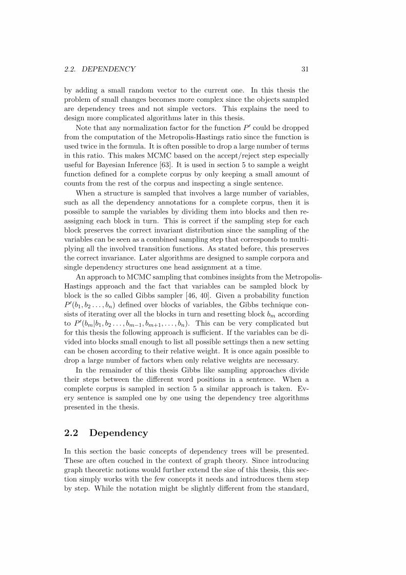
Dependency trees are actual trees in the graph theoretic sense. Theyare of great interest because they express the already mentioned preferencefor an internal hierarchy and they greatly restrict the number of possiblesettings. They also express the very natural idea that a word should notsemantically modify itself or be the reason for its own grammaticality. Oneexample for a dependency tree is given in figure 2.3. In general edges aredrawn pointing from a head to its children.
Another interesting restriction is that to single roots. The constraintonce again reduces the number of possible dependency structures and alsoexpresses a general linguistic idea. The idea is that there is a single wordthat introduces the theme of the sentence. The restriction is also used as atool to guide the learning of dependency trees in chapter 5.
Definition 11 (Single Rooted Dependency Tree). A dependency tree iscalled Single Rooted if there is only a single word that has the artificial root
34 CHAPTER 2. BACKGROUND
The janitor cleaned the dirty bathroom ROOT
Figure 2.3: An example of a dependency tree.
node as its head. The set of all head assignment functions for a sentence sresulting in a single rooted tree is denoted by Hsingle
s .
There is a general tendency of words to be connected to form consecutivesequences in the sentence. This is expressed through the concept of projec-tive trees. Dependency trees in a corpus, annotated by linguistic expertsusually are either projective or are very close to being projective [59, 84].This can once again be exploited to guide dependency learning and reducethe number of possible structures.
Definition 12 (Crossing Edges and Projective Trees). Assume that thereis an edge e between the words in position i and j and another called e′
between the positions k and l. e and e′ are said to be crossing edges if it istrue that one edge points between the other, in other words if the positionscan be ordered such that e1 < e′1 < e2 < e′2 ∨ e′1 < e1 < e′2 < e2 were e1
and e2 are either i or j and e′1 and e′2 are either k or l. If a dependencytree 〈s, h〉 has no crossing edges, then it is called projective. A crossingedge is also called a non-projective edge. The set of all head assignmentsleading to projective trees for a sentence s is denoted by Hprojective
s . The setof all assignments that lead to single rooted, projective trees is denoted byHprojective+single
s . Note that edges between the artificial root and other wordsare also candidates for crossing edges.
Note that this results in very strong and complex relationships betweenthe edges within a tree. If two words are connected by an edge then thewords in between them only have a very restricted choice of heads. In figure2.4 this is illustrated. The only way that the given dependency tree canbe completed to create a projective structure would be to assign “janitor”either the head “The” to its left, or the head “cleaned” to its right. Thisalso explains why it may be helpful for learning to demand that there areno crossing edges. The possible choices that can be made once a few headsare decided on are often strongly limited.
It should also be clear why it is hard to sample only projective trees, atleast as long as the dependency structures are supposed to be changed bymany subsequent small changes. The following chapters will show that thisis actually possible without any clever re-parametrization of the problem[67].

2.2. DEPENDENCY 35
The janitor cleaned the dirty bathroom ROOT
Figure 2.4: An example of how the restriction to projective dependencytrees can limit the possible heads for a word.
This very short introduction to the concepts of dependency is actuallyall that will be needed in this thesis. The interested reader is encouraged toconsult the references mentioned in the text.

36 CHAPTER 2. BACKGROUND
Chapter 3
Sampling Dependency Treeswith Markov Chain MonteCarlo
3.1 Introduction
This chapter presents MCMC methods for the principled sampling of de-pendency trees. In section 3.3 some simple algorithms are developed thathandle the sampling of dependency trees with very little implementationeffort. This raises the question why it would be necessary to focus a lot ofattention on the sampling of dependency trees. The answer is twofold. Thefirst point is the idea that a single sampler will not perform well for all pos-sible distributions over dependency trees. For each distribution there will besamplers likely to get “stuck” in local modes. Other samplers will be able tomove from mode to mode more easily. Different samplers will also have dif-ferent requirements in the amount of computational resources they require1.The second and more interesting reason for developing more sophisticatedapproaches to sampling is an interest to introduce structural restrictions intoa sampling process. One example for this is restricting sampled trees to beprojective. These restrictions can be helpful in the induction of dependencytrees since they allow for the incorporation of linguistic knowledge that mayguide a learning process [69, 106, 101]. Later it is also shown that restrict-ing the explored set can aide an MCMC process substantially. But whenonly trees with a certain restriction are allowed, then this could underminethe convergence of samplers. In chapter 2 it was seen that irreducibility isnecessary to ensure convergence. If the trees to be sampled are severely re-stricted, then irreducibility becomes harder to establish. Constraints couldalso make the problem of “getting stuck” more pronounced. This means that
1The algorithms developed here generally differ in the amount of time that is required,while the amount of memory will be similar up to constant factors
37
38 CHAPTER 3. SAMPLING DEPENDENCY TREES WITH MCMC
it is interesting to explore algorithms that deal with all manner of structuralrestrictions. Even though only two constraints are considered in this thesis,solving them provides insight that can inspire techniques for dealing withother types of constraints. Specifically these restrictions are to projectiveand single rooted trees. For every problem some alternatives are discussed.They differ in the way they explore the search space and in the resourcesthey require. The following sections give an discussion of the state of the isand the different algorithms. Before this is done a short discussion of thetwo structural restrictions is given.
There is an important divide in the research on algorithms for depen-dency structures [59]. One line of investigation focuses on unrestricted de-pendency trees. Algorithms in this setting are usually only feasible understrong independence assumptions [74, 92]. Another group of contributionsis focused on working with projective dependency trees. Recall that such atree has no crossing edges. This second line of research is interesting becausethe added constraint tends to make estimation and optimization problemseasier to solve by dynamic programming [32]. Previous research has shownthe “amount” of non-protectiveness in a corpus of annotated sentences tousually be fairly moderate[84]. This means that at most a few of the edgesfor every parse tree will cross. It would be natural to take this as basisfor the hypothesis that restricting machine learning algorithms to projectivetrees could be helpful. In fact a great deal of the literature on the unsuper-vised learning of dependency trees has made use of precisely this restriction[57, 22, 102, 110, 45]. At the same time there are algorithmic problemsthat can be more efficiently solved when the set of admissible solutions isextended to include non-projective dependency structures. Finding an op-timal unrestricted dependency tree can be achieved in quadratic time if theweight of each tree can be calculated by multiplying weights assigned tosingle edges [73, 74]. In this scenario it is said that the weight is edge fac-tored. Solving the optimization problem for trees that are not edge factoredis usually much NP-hard [74]. Algorithms that only consider projective treescan handle more complex weight definitions. It can be concluded that thereis no option that is universally more efficient. The best choice depends onthe intended application. A similar statement concerning projective andnon-projective dependency trees could be made with regard to the qualityof the dependency parsing results that are achieved in the literature. Twoof the most well known dependency parsers are the MST parser and theMalt parser [75]. They have performed very well in shared tasks. The MSTparser is a non-projective dependency parsers that requires weights to factoralong the edges. The Malt parser is based on projective dependency parsingand constructs the parse tree step by step in a type of greedy search. Sinceboth approaches seem to have a number of benefits it seems reasonable toinvestigate them both in this work.
This thesis also introduces global sampling steps. One of the two pre-
3.1. INTRODUCTION 39
sented methods is geared towards a specific setting: For the case in whichtrees are not restricted to projective structures a MCMC algorithm is givenwhich is able to change most of the edges in a tree at the same time. Thisrequires the ability to derive an edge factored distribution which approx-imates the distribution of interest sufficiently well. “Sufficiently well” isof course defined by the performance desired. There are some very simplealgorithms that can be employed to propose a tree from from such an ap-proximation. The drawback of the algorithm is its inability to deal withstructural restrictions to the dependency trees.
This thesis will also develop a general algorithm which can quite grace-fully deal with all types of structural restrictions. This is done by extendingthe idea of greedy processing in a way that allows for correct MCMC sam-pling. The algorithm also makes use of an approximation to the weightfunction. Which approximation is simpler to construct will depend on thethe model used. The algorithm can also be adapted arbitrarily to any func-tion since there is no requirement for edge factoring.
All algorithms developed here do not require more resources than a sim-ple Gibbs sampler, up to a constant factor. This can be seen by comparisonto the Gibbs techniques developed for both the projective and non-projectiveapplication scenarios. One hopes for the global algorithms to have a simpleadvantage over the local version: being able to make “greater” steps in thespace of possible parse trees and escape local optima. Finally some verysimple algorithms, based on uniformly changing edges in a dependency tree,are presented for projective and non-projective dependency parsing. Thesealgorithms have the benefit of using a small amount of computational re-sources in every sampling step. At the same time they may take a largernumber of steps in order to correctly estimate values of interest.
Aside from the projective/non-projective divide, the second structuralrestriction considered in this section is sampling with only a single child forthe artificial root node. This problem is interesting for the prediction ofdependency trees since it makes the definition of models simpler, especiallyin an unsupervised setting. Without this restriction the degenerate case ofall words attaching to the artificial root could easily occur for many models.This happens because the artificial root is present in every sentence andmodels will often rely on frequent co-occurrence between a potential headand child in order to score a possible dependency tree. In research by Brody[12] exactly this problem occurred and had to be handled by parameter tun-ing. Research by Marecek and Zabokrtsky [69] on unsupervised dependencyparsing suggested the single root constraint as a way to deal with this prob-lem. It is also true that a single root per sentence is a good heuristic in shortsentences. Consider the corpora from the 2012 PASCAL challenge on unsu-pervised dependency parsing, which are discussed in chapter 5. Figure 3.1shows that once a corpus has been reduced by removing punctuation and
40 CHAPTER 3. SAMPLING DEPENDENCY TREES WITH MCMC
only using sentences of length 10 or less2, the majority of sentences onlyhave a single root. Only for Dutch and Slovene have comparable numbersfor multiply and single rooted sentences. Using such a reduced version of acorpus is a very frequent setting for the evaluation of unsupervised learningfor dependency parsing. Not allowing for more than one node to attach tothe artificial root also implies the salient guideline that most words in a sen-tences should have a head with actual syntactic and semantic content. Asidefrom these reasons there is also the fact that this is one instance of a moregeneral problem. The way it is solved is basically through an “exchange” ofedges. This mean that any constraint of the form “there must be x edges oftype y” could be handled this way. While no additional restrictions are con-sidered here, the research is essentially a basis to incorporate many otherrestrictions without sacrificing irreducibility. Thanks to the very generalformulation of the Metropolis-Hastings approach it is possible to deal withnearly all distributions that one may come up with as long as it is possible to“efficiently” compute the value of the weight function for single trees up toa normalization constant. This means that establishing irreducibility andgenerating good proposals are the two main topics that need to be dealtwith. Making it easy to solve the former for dependency trees is one of themain topics of this work.
The remainder of this chapter is structured as follows. A review ofthe state of the art is given in section 3.2. There has been some initialresearch in the field, but some very interesting problems are still left tobe solved. Section 3.2 also discusses some of the alternative algorithms forcomputing expectations and other features of distributions over dependencytrees. Section 3.3 starts with the introduction of simple Gibbs style anduniform samplers that can be used as an out of the box solution for MCMCon dependency trees. These are extended with larger steps in section 3.4.In the subsection 3.4.1 an algorithm is introduced that makes use of anapproximate distribution to potentially change most of the dependenciesin a sentence at the same time. This algorithm results from work on thesampling of spanning trees done by Wilson [117]. A technique for greedilyconstructing new proposals is given in subsection 3.4.2. The two constraintsthat this work is concerned with are discussed in subsections 3.3.3 and 3.3.4.
3.2 State of the Art
The main goal of this section is to introduce some of the existing research onthe sampling of dependency annotation. Since subsequent chapters intro-duce alternative approaches to this problem it is only natural to discuss someof the advantages and shortcomings of the older algorithms. This includesthe types of distributions for which the different samplers are intended as
2A setting explained in more detail in chapter 5.
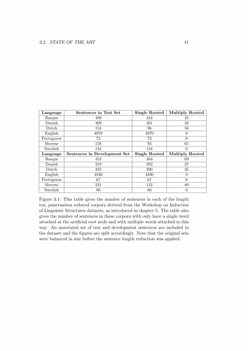
3.2. STATE OF THE ART 41
Language Sentences in Test Set Single Rooted Multiply RootedBasque 489 444 45Danish 409 361 48Dutch 154 96 58
English 4970 4970 0Portuguese 73 73 0
Slovene 158 93 65Swedish 134 134 0
Language Sentences in Development Set Single Rooted Multiply RootedBasque 453 384 69Danish 319 292 27Dutch 325 290 35
English 4830 4830 0Portuguese 67 67 0
Slovene 221 132 89Swedish 80 80 0
Figure 3.1: This table gives the number of sentences in each of the lengthten, punctuation reduced corpora derived from the Workshop on Inductionof Linguistic Structures datasets, as introduced in chapter 5. The table alsogives the number of sentences in these corpora with only have a single wordattached at the artificial root node and with multiple words attached in thisway. An annotated set of test and development sentences are included inthe dataset and the figures are split accordingly. Note that the original setswere balanced in size before the sentence length reduction was applied.

42 CHAPTER 3. SAMPLING DEPENDENCY TREES WITH MCMC
well as their demands in terms of computational resources.The oldest reference using MCMC to approximate probability distribu-
tions over dependency trees, to the knowledge of the author, is the work byNakagawa [78]. In it Gibbs sampling is used with very little remarks madeabout the actual sampling algorithm. Some information can be gleaned fromthe features used. The weighting scheme makes use of binary features indi-cating whether a dependency structure is acyclic and features that indicatewhether the tree is projective or not. This suggest that the sampler operatesonly on the head assignments for words and that these can always be setto any other position in the sentence, regardless of whether this forms a de-pendency tree or not. This could mean that sampling operates on the moregeneral concept of a dependency structure. Therefore solving the problemwith a Gibbs sampler becomes trivial. The sampling can proceed by iterat-ing over the words in a sentence or in a complete corpus. The head variableof a word is then re-sampled by calculating the un-normalized weight forevery possible head in the sentence and constructing a multinomial. Fromthis multinomial a new head can be drawn. While this approach would bevery easy to implement, it has the obvious drawback of not making much useof any linguistically motivated structure for dependencies. Ignoring struc-tures that do not constitute trees has the potential to increase the speedwith which the space of possible assignments can be explored. A potentialthat is not exploited by this simple sampler. In the subsequent sections itwill be seen that this is a simple problem to fix. It will also be argued thatit is easy to decide during each sampling step which assignments do forma tree and which do not. This work elaborates on the simple approach byestablishing correctness even for restricted structures, showing how checkingfor treeness can be completely avoided and, in later chapters, attempting aninvestigation into the effectiveness of the approach.
A more detailed discussion of the sampling problem is given by Marecekand Zabokrtsky [69]. For their investigation they also make use of the “sim-ple” Gibbs sampler discussed before. The underlying structure they use aredependency structures. For each word a new head is sampled in turn withoutregard for whether this does result in a valid dependency tree. They extendthe approach of Nakagawa [78] by ensuring that the structures that are sam-pled have a single word attached at the artificial root and form trees. Thisis done by checking whether a dependency assignments conforms with theseconstraints after each unrestricted Gibbs sampling step. If the head choicesform a dependency tree and have only a single node attached at the artificialroot, then sampling proceeds normally, otherwise Marecek and Zabokrtsky[69] tackle this problem by using an additional step. Whenever a cycle iscreated, one of the nodes in the cycle is chosen and immediately re-sampled,this time with the constraint that the resulting structure must be acyclic.The same is done in case the single root constraint is violated. One of theviolating nodes is selected and re-sampled under the restriction that the
3.2. STATE OF THE ART 43
resulting structure may only have a single root. Marecek and Zabokrtsky[69] do not provide a proof of the correctness of the sampler. The algorithmlooks like a standard Gibbs sampler at a first glance but there are basicallytwo different weight functions used during sampling. One assigns weight toill formed structures, while the other gives zero weight to them. This mixingof distributions would make a proof desirable. The algorithm also requiresthat it is checked after each step whether the resulting structure forms atree. As stated already, it is just as easy to ensure that only correct struc-tures are considered without checking, at least as long as a head by headapproach is taken. The algorithm by Marecek and Zabokrtsky [69] also hasthe problem that weight has to be assigned to the multiply rooted structuresto ensure irreducibility. This might not be in the interest of the designer ofa model. If a weight function is based on using a single, identifiable root,then it would be necessary to come up with some form of smoothing. Thissmoothing would be non-trivial since it would have to be strong enough tooccasionally allow for words to be attached at the artificial root and makean exchange possible, while also not leading to the overly frequent creationof those attachments. The idea of sampling single rooted structures is takenup here and special “root sampling steps” are developed that do not requireany illegal intermediate structures and are argued to be just as powerful asthe immediate restricted re-sampling step.
In reviewing the sampling of non-projective dependency trees there seemsto be a lack of any approach that only explores valid dependency trees andis provably convergent. This is a field that could still use some attentionand it is one contribution of this work to provide multiple provably correctsamplers for non-projective dependency trees.
There is a larger body of work that deals with the sampling of projectivestructures in contrast to the unrestricted problem discussed so far. Manyof the approaches are based on sampling from a chart that has been con-structed using an approximate distribution. The technique is based on ascheme introduced for constituency structures by Chappelier and Rajman[17]. They proposed this technique to deal with optimization in a Data Ori-ented Parsing setting [9]. The algorithm was employed in an unsupervisedlearning setting by Johnson et. al. [56]. The approach can be extended todependency parsing by using the chart construction algorithm introducedby Eisner [32, 115, 68] or by using a projection from constituency trees todependency trees [8]. Since the algorithm relies on dynamic programmingover sub-spans of the sentence, it has only been applied to projective prob-lems. It is implemented as follows. An item chart for increasingly largerspans in the sentence is constructed for an approximate distribution withindependence features well suited for dynamic programming. This is usuallydone in the style of the Eisner algorithm or the CYK algorithm [119]. Thereis a difference in runtime and capabilities between the the Eisner algorithm[32] and algorithms based on using constituency trees and a projection. The

44 CHAPTER 3. SAMPLING DEPENDENCY TREES WITH MCMC
Eisner algorithm is faster, but assumes that edges on either side of a headare independent. The complete chart can be used to derive expectationsfor every possible head assignment a word may have, similar to the wayconstituent expectations are computed in the Inside-Outside algorithm [61]or transition expectations in the Forward-Backward algorithm [4]. The sim-plest way to use this3 is to draw a head for the first word according to thisexpectation, then use the expectations given the first choice4 for the assign-ment of the second word and so on until a complete dependency structureis drawn. Since the chart contains the probabilities of trees according tothe approximate distribution, trees are proposed accordingly. This meansthat a good approximate distribution proposes trees with probability closeto proportional to their actual weight. It is also be easy to compute theprobability prop(t) with which a tree t is proposed by simply checking thechart. Therefore it is very straightforward to use the Metropolis-Hastingsrule with the acceptance probability given by:
pa(t′|t) =prop(t)p(t′)
prop(t′)p(t)(3.1)
The approach has two main drawbacks. The first is the fact that even themost efficient of the dynamic programming based approaches for projectivedependency trees, Eisners algorithm, has a running time in O(n3) weren is the number of words in the sentence. The second is the fact thatit is necessary to design an approximate distribution conforming with theindependence assumptions the dynamic programming algorithms make. It isof course always possible to reduce the independence assumptions by usinga more complex dynamic programming algorithm. The clear advantage ofthe technique is the fact that it can sample from almost exactly the desireddistribution, if a good approximation can be found. Sampling from a chartalso has the advantage of being the most feasible solution to the problemof global sampling steps. A good approximate distribution means that thewhole tree can be reset in a single step and there is still a good chanceof accepting the new proposal. For this reason ideas are explored whenglobal steps are proposed in this thesis. The first is an extension of theparadigm to non-projective trees. The foundation of the second is alreadylaid in the way the chart sampling was presented here. It considers usingsome auxiliary distribution to construct a complete dependency parse stepby step, resulting in a generalization that allows for the use of charts or anyother distribution for this task. The step by step version makes it possibleto consider ever more information when the tree is constructed.
In another paper by Marecek and Zabokrtsky [70] and also in the thesisof Mareccek [67] an additional approach was introduced. Like some of the
3Actual implementations may vary in the order in which edges are created4Usually also easily derived from the chart.
3.2. STATE OF THE ART 45
techniques based on constructing a chart of possible solutions, this approachrelies on the fact that a projective dependency parse can be mapped to aconstituency tree. The mapping they use is illustrated in figure 3.2. For eachword there is one constituent that directly subsumes this it. For some wordw call this constituent cw. cw directly subsumes the constituent cw′ for allwords w′ which are children of w in the dependency tree. Sampling is thenimplemented by removing single constituents and doing a Gibbs samplingstep over all the possible ways a new constituent could be added. In otherwords this means that one of the children of a word can become its headand/or both exchange children. While this method does not require anyauxiliary distribution, it is quite possible that this algorithm can becomestuck in a local optimum just like any other local approach. This is par-ticularly problematic since the number of function evaluations that is donefor re-sampling a single word is in O(n2) were n is the number of words ina sentence. To see that this is the case consider a completely flat depen-dency tree in which all words are children of a single root node. When aword other than that root is sampled then any span of words in the sen-tence would correspond to a possible new solution. The number of spansis in O(n2) meaning that re-sampling the complete tree by re-assigning thespan for each word may need a number of evaluations in O(n3). Therebyeasily leading to a runtime that is much worse than the time used by thechart based approach because the O(n3) evaluations used by the chart basedapproach are usually made from a much simpler function. Because of thishigh price, this sampler is not consider further.
As far a the sampling of projective trees is concerned the following state-ment could be made: if there is a good approximate distribution that canbe easily used in a dynamic programming based approach, then this canlead to a sampler that converges very fast and is not very prone to beingstuck in local modes. The latter being the case since a completely new treeis constructed each time a sampling step is taken. If there is no way toconstruct a good approximation, then the algorithm based on charts mayperform just as bad as proposing trees uniformly at random. The approachby Mareccek [67] is not dependent on any approximation, but it may re-quire more runtime and could become stuck in a local optimum since it onlychanges a few of the heads at a time. Note that the fact that it is possibleto map dependency structures to constituency structures would also makeit possible to employ alternative approaches to the sampling of constituencytrees to dependencies. One example for such an approach would be the al-gorithm introduced by Chung et. al. [20] that samples constituency treesbased on a hyper-graph representation. Another is the algorithm by Zhaiet. al [120] that relies on “flipping” constituents in a binary tree. At thesame time it is required to not distort the original distribution by allowingmore representations for one dependency tree than for another. If this isnot considered then it could easily be problematic because of the fact that
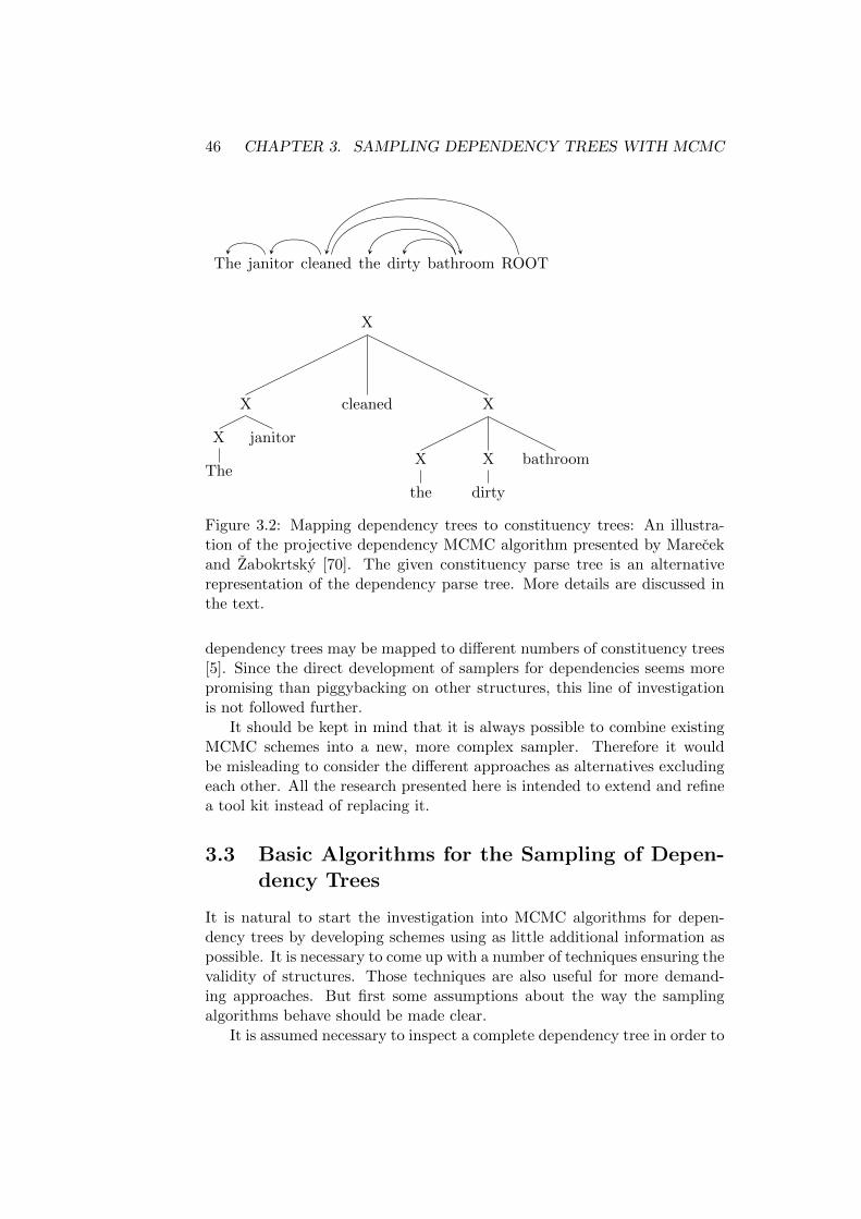
46 CHAPTER 3. SAMPLING DEPENDENCY TREES WITH MCMC
The janitor cleaned the dirty bathroom ROOT
X
X
X
The
janitor
cleaned X
X
the
X
dirty
bathroom
Figure 3.2: Mapping dependency trees to constituency trees: An illustra-tion of the projective dependency MCMC algorithm presented by Marecekand Zabokrtsky [70]. The given constituency parse tree is an alternativerepresentation of the dependency parse tree. More details are discussed inthe text.
dependency trees may be mapped to different numbers of constituency trees[5]. Since the direct development of samplers for dependencies seems morepromising than piggybacking on other structures, this line of investigationis not followed further.
It should be kept in mind that it is always possible to combine existingMCMC schemes into a new, more complex sampler. Therefore it wouldbe misleading to consider the different approaches as alternatives excludingeach other. All the research presented here is intended to extend and refinea tool kit instead of replacing it.
3.3 Basic Algorithms for the Sampling of Depen-dency Trees
It is natural to start the investigation into MCMC algorithms for depen-dency trees by developing schemes using as little additional information aspossible. It is necessary to come up with a number of techniques ensuring thevalidity of structures. Those techniques are also useful for more demand-ing approaches. But first some assumptions about the way the samplingalgorithms behave should be made clear.
It is assumed necessary to inspect a complete dependency tree in order to
3.3. BASIC ALGORITHMS 47
derive the weight it has. Since weights are generally only needed up to someshared factor, some models may make it possible to compute the necessaryvalues by simply inspecting a portion of the dependency tree. This could beespecially true if only a single edge is changed. These specific optimizationsare not considered here, since the main goal is to develop algorithms whichcan be used for a large range of models. This consideration also goes theother way. While all the samplers are presented here in the context of singletrees, they can obviously be used for inference with whole corpora by apply-ing them to different sentences in turn. This follows from the preservation ofan invariant distribution under multiplication. The weight function for eachtree would then be the weight for the complete corpus with the assumptionthat it is possible to derive the necessary relative weights from an inspectionof the tree in question and some statistics summarizing the current state ofhidden variables in the remainder of the corpus. If deriving the necessaryrelative weight requires iterating through the complete corpus, then it wouldmost likely be necessary to update a larger number of structures at the sametime or use completely different approximation techniques, because iterat-ing over the complete corpus to sample a single edge seems excessive. Whilethe assumption is made that it is only necessary to inspect at most a smallnumber of sentences and some general statistics, this does not imply that theevaluation of the weight is necessarily fast and generally evaluations of theobjective function will dominate the computation. The number of functionevaluations that need to be made before a sampler converges is thereforea good indicator of the runtime properties the algorithm will have. Theweight function or some auxiliary version of it are also usually called in theinnermost loop of any algorithm. This means that the number of calls tothis function indicates the general runtime of a MCMC scheme. Because ofthis the efficiency of the algorithms is generally measured by the number offunction evaluations they require. With this initial explanation out of theway, the first step is developing tools that ensure that a sampled dependencyassignment is always a tree. This can then be extended in order to ensureother constraints. Since a head by head approach is taken initially, thisreduces to making sure that the proposed heads are viable. The techniquecan then be used in global steps to ensure the same during the constructionof a tree.
3.3.1 Ensuring Treeness and Other Constraints
This section presents a number of algorithms used repeatedly to ensure thatthe dependency structures conform to certain constraints. There are twoways that such restrictions could be enforced. The first would be to “sim-ply” consider any structure and reject those that do not follow the desiredconstraint. One way of doing this would be to simply set the weight forthose non-conforming assignments to 0 and let the accept/reject step of the
48 CHAPTER 3. SAMPLING DEPENDENCY TREES WITH MCMC
Metropolis-Hastings approach do the rest. This implies testing each pro-posed assignment individually for whether it is admissible. Consider this inthe setting of a Gibbs sampler that attempts to re-assign the head for everyword in the corpus. This sampler would calculate the weight for every possi-ble position to be the head for the word that is currently being re-assigned.If every calculation needs to check the complete graph in order to ensure aconstraint like the restriction to trees, then this implies a cubic number ofsteps devoted to checking for every sweep over the complete sentence. Asstated before, it will be assumed that the evaluation of the weight functiondominates the runtime of all samplers, but it could still be helpful to de-velop a more efficient approach to ensuring constraints. Not considering anystructures that violate relevant constraints is another approach for ensuringrestrictions. This technique is the one used here. It means that the con-straints become part of the sampling algorithm themselves instead of beingexpressed in the form of the weight function. This does carry with it thepossibility for better performance. Especially since the number of settingsinspected is potentially reduced. In order to design algorithms that onlypropose valid structures, it is necessary to compute the viable heads for aword given a set of other head assignments. Since some of the algorithmsintroduced later make use of incomplete head assignments, i.e. assignmentsin which no head is designated for some words, the algorithms presentedhere need to be able to deal with this type of assignments. This subsectionconcerns itself with algorithms that compute viable candidate heads. Latersubsections use these candidates to derive complete samplers and show thatthese samplers are correct.
The most basic requirements for a sampler of dependency trees is that itactually samples dependency trees, i.e. that the head assignments proposedactually correspond to tree graphs. It is generally assumed that the start-ing point for sampling is either a valid dependency tree or an incompleteassignment that can be extended in order to generate a dependency tree.In the incomplete case this implies that there are no loops in the structuregenerated so far. With this simple assumption it is possible to compute allthe viable head candidates for a word in linear time. This can be achievedquite easily by using algorithm 1. The algorithm simply finds all the wordsthat are descendants of the position for which a new head is chosen. Sinceattaching the word to any of these would create a loop, they are excludedas candidates. The algorithm given here uses an iterative, breadth-firstapproach. It could just as easily be implemented by applying a recursiveand/or depth first approach. Note that finding the children of a position inline 7 usually requires keeping track of the inverse of the head assignmentfunction. Keeping this inverse function and creating a list of possible headsrequires linear memory. Since the storing of any actual head function alsorequires linear memory, this does not seem like a substantial extension ofthe needed memory. Note that the positions in the List L are counted from

3.3. BASIC ALGORITHMS 49
0 and that the sentence length is assumed to not include the artificial rootnode.
Algorithm 1 FindPossibleHeads(WordPosition p, IncompleteHeadAssign-ment h, SentenceLength l, ArtificalRootPosition r)
1: heads← {n|0 < n ≤ l} ∪ {r}2: L← makeEmptyList3: append p to L4: i = 05: while i < length(L) do6: p′ ← ith entry of L7: for all p∗ ∈ {q|h(q) = p′} do8: append p∗ to L9: heads← heads− {p∗}
10: end for11: i← i+ 112: end while13: return heads
Since dependency trees are the basic structure considered here, algorithm1 can now be extended in order to allow for additional structural limitations.The single root restriction is the first addition. Incorporating this constraintinto algorithm 1 is relatively straightforward. There are three possible cases.If the word for which new heads are sampled is currently attached to theartificial root node, then the only possible assignment for its head has to bethe artificial root node. Otherwise the head assignments would no longerconstitute a dependency tree, since all other heads must be children of theroot. If the node that is currently being sampled is not attached at theartificial root, but some other node is, then the node being sampled cannotattach at the artificial root without violating the the single root constraint.If the node being sampled is not attached at the root but there is no othernode attached at the root5 then it should be possible to attach the nodeat the root. This leads to algorithm 2. Note that, while this algorithmwill form the basis of sampling single rooted trees later in this chapter, it isnot sufficient to just compute the legal head assignments according to thisalgorithm for each word and then choose one among them. The reason forthis is the fact that a sampler on this basis would never change the rootnode that has been chosen. Additional steps ensuring that all possible treesare sampled are introduced in subsections 3.3.3 and 3.3.4.
Ensuring that a tree is projective is somewhat more complex than ensur-ing that a tree only has a single root. For a given word position p and headposition p′ the easiest way of checking that using p as a head for p′ does
5This will only occur in the more complex algorithms that construct a complete tree.
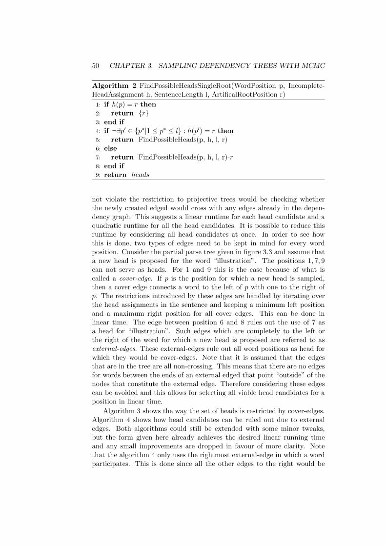
50 CHAPTER 3. SAMPLING DEPENDENCY TREES WITH MCMC
Algorithm 2 FindPossibleHeadsSingleRoot(WordPosition p, Incomplete-HeadAssignment h, SentenceLength l, ArtificalRootPosition r)
1: if h(p) = r then2: return {r}3: end if4: if ¬∃p′ ∈ {p∗|1 ≤ p∗ ≤ l} : h(p′) = r then5: return FindPossibleHeads(p, h, l, r)6: else7: return FindPossibleHeads(p, h, l, r)-r8: end if9: return heads
not violate the restriction to projective trees would be checking whetherthe newly created edged would cross with any edges already in the depen-dency graph. This suggests a linear runtime for each head candidate and aquadratic runtime for all the head candidates. It is possible to reduce thisruntime by considering all head candidates at once. In order to see howthis is done, two types of edges need to be kept in mind for every wordposition. Consider the partial parse tree given in figure 3.3 and assume thata new head is proposed for the word “illustration”. The positions 1, 7, 9can not serve as heads. For 1 and 9 this is the case because of what iscalled a cover-edge. If p is the position for which a new head is sampled,then a cover edge connects a word to the left of p with one to the right ofp. The restrictions introduced by these edges are handled by iterating overthe head assignments in the sentence and keeping a minimum left positionand a maximum right position for all cover edges. This can be done inlinear time. The edge between position 6 and 8 rules out the use of 7 asa head for “illustration”. Such edges which are completely to the left orthe right of the word for which a new head is proposed are referred to asexternal-edges. These external-edges rule out all word positions as head forwhich they would be cover-edges. Note that it is assumed that the edgesthat are in the tree are all non-crossing. This means that there are no edgesfor words between the ends of an external edged that point “outside” of thenodes that constitute the external edge. Therefore considering these edgescan be avoided and this allows for selecting all viable head candidates for aposition in linear time.
Algorithm 3 shows the way the set of heads is restricted by cover-edges.Algorithm 4 shows how head candidates can be ruled out due to externaledges. Both algorithms could still be extended with some minor tweaks,but the form given here already achieves the desired linear running timeand any small improvements are dropped in favour of more clarity. Notethat the algorithm 4 only uses the rightmost external-edge in which a wordparticipates. This is done since all the other edges to the right would be
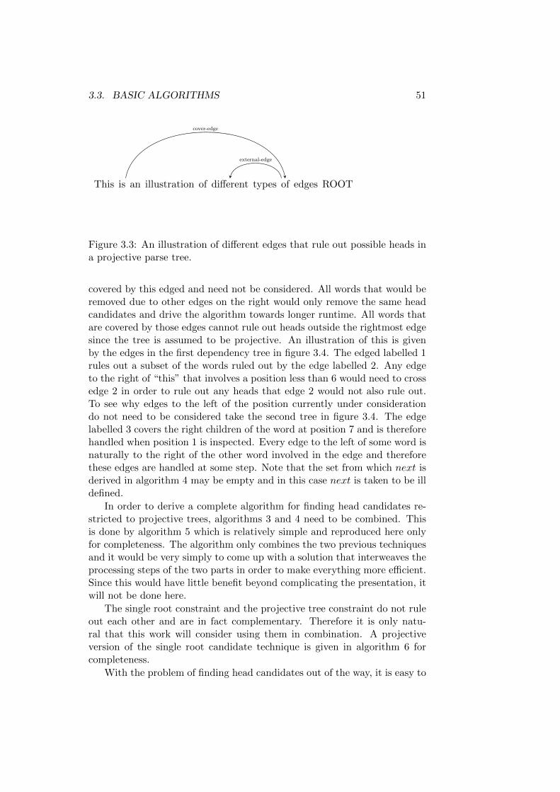
3.3. BASIC ALGORITHMS 51
This is an illustration of different types of edges ROOT
cover-edge
external-edge
Figure 3.3: An illustration of different edges that rule out possible heads ina projective parse tree.
covered by this edged and need not be considered. All words that would beremoved due to other edges on the right would only remove the same headcandidates and drive the algorithm towards longer runtime. All words thatare covered by those edges cannot rule out heads outside the rightmost edgesince the tree is assumed to be projective. An illustration of this is givenby the edges in the first dependency tree in figure 3.4. The edged labelled 1rules out a subset of the words ruled out by the edge labelled 2. Any edgeto the right of “this” that involves a position less than 6 would need to crossedge 2 in order to rule out any heads that edge 2 would not also rule out.To see why edges to the left of the position currently under considerationdo not need to be considered take the second tree in figure 3.4. The edgelabelled 3 covers the right children of the word at position 7 and is thereforehandled when position 1 is inspected. Every edge to the left of some word isnaturally to the right of the other word involved in the edge and thereforethese edges are handled at some step. Note that the set from which next isderived in algorithm 4 may be empty and in this case next is taken to be illdefined.
In order to derive a complete algorithm for finding head candidates re-stricted to projective trees, algorithms 3 and 4 need to be combined. Thisis done by algorithm 5 which is relatively simple and reproduced here onlyfor completeness. The algorithm only combines the two previous techniquesand it would be very simply to come up with a solution that interweaves theprocessing steps of the two parts in order to make everything more efficient.Since this would have little benefit beyond complicating the presentation, itwill not be done here.
The single root constraint and the projective tree constraint do not ruleout each other and are in fact complementary. Therefore it is only natu-ral that this work will consider using them in combination. A projectiveversion of the single root candidate technique is given in algorithm 6 forcompleteness.
With the problem of finding head candidates out of the way, it is easy to

52 CHAPTER 3. SAMPLING DEPENDENCY TREES WITH MCMC
This is an illustration of different types of edges ROOT
1
2
This is an illustration of different types of edges ROOT
3
1
2
Figure 3.4: An illustration of different edges used to explain algorithm 4.
Algorithm 3 FindCoverEdgeReduction(WordPosition p, Incomplete-HeadAssignment h, SentenceLength l, ArtificalRootPosition r)
1: min← 12: max← l + 13: i← 14: h(p)← undefined5: while i ≤ l do6: if h(i) is not defined then7: i← i+ 18: else9: head = h(i)
10: if i < p ∧ p < head then11: min← max(min, i)12: max← min(head,max)13: else14: if i > p ∧ p > head then15: min← max(min, head)16: max← min(i,max)17: end if18: end if19: i← i+ 120: end if21: end while22: heads← {i|min ≤ i ≤ max}23: return heads

3.3. BASIC ALGORITHMS 53
Algorithm 4 FindExternalEdgeReduction(WordPosition p, Incomplete-HeadAssignment h, SentenceLength l, ArtificalRootPosition r)
1: heads← {i|1 ≤ i ≤ l}2: i← 13: h(p)← undefined4: while i < l do5: if h(i) is not defined then6: i← i+ 17: else8: if i < p then9: next← max {j|(h(j) = i ∨ h(i) = j) ∧ j < p ∧ j > i}
10: else11: next← max {j|(h(j) = i ∨ h(i) = j) ∧ j > i}12: end if13: if next is well defined then14: heads← heads− {j|i < j < next}15: i← next16: end if17: end if18: end while19: heads← heads ∪ {r}20: return heads
Algorithm 5 FindProjectiveHeadCandidates(WordPosition p, Incomplete-HeadAssignment h, SentenceLength l, ArtificalRootPosition r)
1: heads← FindCoverEdgeReduction(p, h, l, r)2: heads← heads∩ FindExternalEdgeReduction(p, h, l, r)3: return heads
Algorithm 6 FindPossibleHeadsSingleRootProjective(WordPosition p, In-completeHeadAssignment h, SentenceLength l, ArtificalRootPosition r)
1: if h(p) = r then2: return {r}3: end if4: if ¬∃p′ ∈ {p∗|0 < p∗ ≤ l} : h(p′) = r then5: return FindProjectiveHeadCandidates(p, h, l, r)6: else7: return FindProjectiveHeadCandidates(p, h, l, r)-r8: end if9: return heads
54 CHAPTER 3. SAMPLING DEPENDENCY TREES WITH MCMC
derive some very simple MCMC algorithms for the sampling of dependencytrees. These are given and shown to be correct in the next subsections. Thisincludes a discussion on ways of dealing with single headed structures. Thena section on more complex samplers follows
3.3.2 Gibbs and Metropolis-Hastings Samplers for Depen-dency Trees
This subsection will derive some samplers for dependency structures thatrely on some well known MCMC techniques. The first is a Metropolis-Hastings [40] approach to word by word sampling. This means that thealgorithm sweeps over the words in a sentence and samples the head for eachword in turn much in the way that a Gibbs sampler would. In contrast to aGibbs sampler that would consider all possible settings for each word, thisalgorithm simply chooses one possible head uniformly at random. This mayseem much less efficient than considering all heads and then choosing oneproportional to the weight of the corresponding setting, but a large numberof evaluations can often be saved if most steps would produce no changeat all. In this scenario computing the weight of all possible settings is awaste, if most settings are extremely unlikely to be chosen anyway. Anothersetting in which the algorithm will perform well is a weight distribution thatis close to uniform. In such a setting the way the algorithm proposes newheads is close to what a full Gibbs sampler would do. Before any furtherdiscussion it will be helpful to actually present the sampler in question. Asstated before the algorithms presented here are intended for the sampling ofa single sentence. They can be combined into more complex samplers for acomplete corpus with techniques presented in section 2.1.2. The techniquesare presented as algorithms that change a given head assignment. MCMCwould then proceed by generating the samples s1, s2, . . . , sn by taking thesample sn+1 to be the result of running the algorithm on sn. Algorithm 7is the simplest approach presented in this work. Throughout it is assumedthat the target is a potentially un-normalized weight function P defined overdependency trees.
The algorithm has the restriction that P has to put weight greater than0 on all trees in order ensure convergence. This is the case since only oneedge is changed at every sampling in order to “reach” every other tree.Note that it still has the advantage that no weight needs to be put on non-tree structures6. Later algorithms do not carry this restriction or allow forcertain weaker requirements. In fact it is later shown that it is possible forthe algorithm to work with a function that sets the weight for some trees to0.
For each sampler that is presented in this work a proof is given that a
6They are in fact never visited
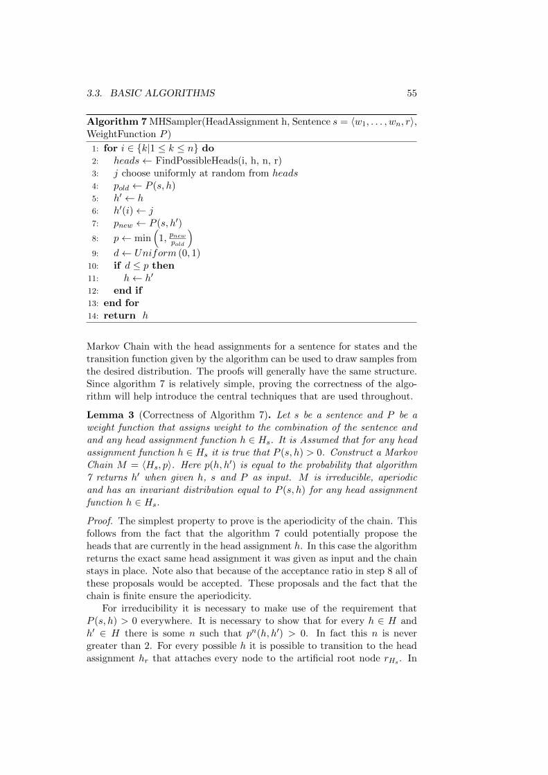
3.3. BASIC ALGORITHMS 55
Algorithm 7 MHSampler(HeadAssignment h, Sentence s = 〈w1, . . . , wn, r〉,WeightFunction P )
1: for i ∈ {k|1 ≤ k ≤ n} do2: heads← FindPossibleHeads(i, h, n, r)3: j choose uniformly at random from heads4: pold ← P (s, h)5: h′ ← h6: h′(i)← j7: pnew ← P (s, h′)
8: p← min(
1, pnew
pold
)9: d← Uniform (0, 1)
10: if d ≤ p then11: h← h′
12: end if13: end for14: return h
Markov Chain with the head assignments for a sentence for states and thetransition function given by the algorithm can be used to draw samples fromthe desired distribution. The proofs will generally have the same structure.Since algorithm 7 is relatively simple, proving the correctness of the algo-rithm will help introduce the central techniques that are used throughout.
Lemma 3 (Correctness of Algorithm 7). Let s be a sentence and P be aweight function that assigns weight to the combination of the sentence andand any head assignment function h ∈ Hs. It is Assumed that for any headassignment function h ∈ Hs it is true that P (s, h) > 0. Construct a MarkovChain M = 〈Hs, p〉. Here p(h, h′) is equal to the probability that algorithm7 returns h′ when given h, s and P as input. M is irreducible, aperiodicand has an invariant distribution equal to P (s, h) for any head assignmentfunction h ∈ Hs.
Proof. The simplest property to prove is the aperiodicity of the chain. Thisfollows from the fact that the algorithm 7 could potentially propose theheads that are currently in the head assignment h. In this case the algorithmreturns the exact same head assignment it was given as input and the chainstays in place. Note also that because of the acceptance ratio in step 8 all ofthese proposals would be accepted. These proposals and the fact that thechain is finite ensure the aperiodicity.
For irreducibility it is necessary to make use of the requirement thatP (s, h) > 0 everywhere. It is necessary to show that for every h ∈ H andh′ ∈ H there is some n such that pn(h, h′) > 0. In fact this n is nevergreater than 2. For every possible h it is possible to transition to the headassignment hr that attaches every node to the artificial root node rHs . In
56 CHAPTER 3. SAMPLING DEPENDENCY TREES WITH MCMC
other words hr(i) = rs for every word position i. This follows from the waythat potential head candidates are computed in algorithm 1. The artificialroot can always be chosen as a head for a word, since all possible trees haveweight greater than zero and there is always a greater than zero chancethat the the artificial head is accepted in step 11. After this the seconditeration step attaches each word to the head chosen for it in the assignmenth′. For each position i the desired head j is either still attached to theartificial root or is at least not a descendant of i. This is the case since jcan not be a descendant of i in h′ if h′ is actually a valid tree. This meansthat j will be among the candidates proposed for i by algorithm 1. Theprobability of accepting this proposal will always be greater than 0 becauseof the requirements on the weight function.
The final statement that needs to be proven is that the chain has thecorrect invariant distribution. This is shown by proving that each single stepin the iteration in line 1 preserves the invariant distribution. The desiredresult then follows from the fact that the multiplication of all the transitionsfunctions preserves the invariant distribution. The invariant distributioncan be shown from the Metropolis-Hastings rule. The rule states that anew state h′ is proposed according to the distribution q(h′|h) and is thenaccepted with probability:
p(h′|h) = min
(1,q(h|h′)P (s, h′)
q(h′|h)P (s, h)
)(3.2)
The proposal distribution is uniform on all the heads that are returnedby algorithm 1. Since the heads returned are the same for h and h′ thismeans that the terms q(h′|h) and q(h|h′) cancel out and the acceptanceprobability reduces to:
p(h′|h) = min
(1,P (s, h′)
P (s, h)
)(3.3)
This is exactly the acceptance probability used in algorithm 7. Theinvariance property follows.
Note that the aperiodicity is usually assured by some state being muchmore probable than all other states and the sampler then stays in this statefor a number of steps. Note that the algorithm could be very inefficientif there are a number of assignments that have high weight and that cannot be reached easily from each other by changing only a single dependencyassignment. It may also take a number of iterations to pick the “correct”head for a word. However the number of evaluations in each iteration issmall and it is possible to exactly predict it if the number of words in the
3.3. BASIC ALGORITHMS 57
corpus is known. Which could be an advantage if there is only a limitedtime budget that can be used for sampling. The amount of memory used islinear for the head candidates that need to be stored and also for the twohead head assignment functions needed.
The extension of this simple sampler to a Gibbs like technique that takesinto consideration the weight of the different possible assignments beforemaking a proposal is a natural next step. This is done in algorithm 8.The sampler does not choose the new head at random. Instead a functionis constructed in the loop in line 4 which is used to give information onthe proportional rate at which heads should be chosen. This means thatthe sampler is basically a Gibbs sampler that is additionally restricted tousing only heads that preserve trees through the use of the algorithm 1.The Sampler requires a larger number of function evaluations per iteration.The sampler 7 would take exactly 2n function evaluations per iteration andsentence. Here n is the length of the sentence for which dependencies arepicked. The number of function evaluations for the sampler 8 may requirea different number of evaluations depending on the structure of the headassignment sampled. This is illustrated by the trees in 3.5. The uppertree in that figure would require 1 evaluation to choose a new head for theword in position 1. This is the case since the only possible head for theposition is the artificial root node. Two evaluations would be required forthe position 2. Since the possible heads are 1 and the artificial root. Therewould be three evaluation for position 3 and so on. This example can beextended to sentences of arbitrary length. Contrast this with the numberof evaluations that are required for the second tree in figure 3.5. For eachposition other than 3 it is necessary to evaluate the objective function for 4possible heads. These heads are the artificial root and the other positionsin the sentence. It can generally be said that the number of evaluationsfor each run of the algorithm 8 are in O(n2). The memory needed is againlinear. Some additional memory is needed to store the function values.
If there is a great disparity between the weight of different head assign-ments then the Gibbs like sampler explores these faster in terms of iterationsthan algorithm 7. The technique still has the problem of easily getting stuckin local optima. This is reflected in that fact that the proof of correctnessfor the sampler again requires that the weight function is greater than 0 ev-erywhere. The intermediate trees required to get from one mode to anothercould have very low probability. A MCMC approach that exchanges largerportions of the tree at once would have a better chance to move quicklythrough the sampling space but may also require more computations. Sam-pling two heads at once would already drive the number of function evalu-ations up to be in the order of O(n4), if every possible pair of assignmentsis considered for every possible pair of positions that could have their headssampled.
The final step in the presentation of algorithm 8 is the proof of its cor-

58 CHAPTER 3. SAMPLING DEPENDENCY TREES WITH MCMC
Algorithm 8 GibbsSampler(HeadAssignment h, Sentence s =〈w1, . . . , wn, r〉, WeightFunction P)
1: for i ∈ {k|1 ≤ k ≤ n} do2: heads← FindPossibleHeads(i, h, n, r)3: h′ ← h4: for head ∈ heads do5: h′(i)← head6: q(head) = P (s, h′)7: end for8: j choose at random proportional to q9: h(i)← j
10: end for11: return h
This is an illustration ROOT
This is an illustration ROOT
Figure 3.5: An illustration of different trees that lead to different requirednumbers of function evaluations by algorithm 8.
3.3. BASIC ALGORITHMS 59
rectness. It is virtually identical to the one given for algorithm 7. The onlymajor difference is the fact that there is no longer an accept/reject stepsin algorithm 8 and it is necessary to show why this still leads to a correctsampler. The idea is the same as the one used in the derivation of the Gibbssampler from the Metropolis-Hastings rule by Norris [85].
Lemma 4 (Correctness of Algorithm 8). Let s be a sentence and P be aweight function that assigns weight to the combination of the sentence andand any head assignment function h ∈ Hs. It is assumed that for any headassignment h ∈ Hs it is true that P (s, h) > 0. Construct a Markov ChainM = 〈Hs, p〉. Here p(h, h′) is equal to the probability that algorithm 8 returnsh′ when given h, s and P as input. M is irreducible, aperiodic and has aninvariant distribution equal to P (s, h) for any head assignment h ∈ Hs.
Proof. The first step is again proving the aperiodicity. It follows from thefact that the function q is greater than zero for every possible head and thecurrent head is always included in the set of possible heads. This wouldallow the sampler to keep moving in place. These movements together withthe finiteness ensure the aperiodicity.
For irreducibility it is necessary to show that for every h ∈ H and h′ ∈ Hthere is some n such that pn(h, h′) > 0. n is again never greater than 2. Forevery possible h it is possible to transition to the head assignment hr thatattaches every node to the artificial root node rs. This follows from the waythat potential head candidates are computed in algorithm 1 and the factthat q will always be greater than zero for the artificial root node because ofthe requirements on the function P . After all words have been attached tothe artificial root, the second iteration step attaches each word to the headchosen for it in the assignment h′. For each position i the desired head j iseither still attached to the artificial root or is at least not a descendant of ijust as before. The probability of the head according to q will again alwaysbe greater than 0.
The final statement that needs to be proven is that the chain has thecorrect invariant distribution. This will be again be proven by showing thateach single step in the iteration in line 1 preserves the invariant distribution.The invariant distribution results from the Metropolis-Hastings rule. Therule demands that a new state h′ is proposed according to the distributionq(h′|h) and is then accepted with probability:
p(h′|h) = min
(1,q(h|h′)P (s, h′)
q(h′|h)P (s, h)
)(3.4)
Here q(h′|h) = P (s,h′)Z with some normalizer Z which can be computed
by adding over the possible settings for the single head currently sampled.This means that the Metropolis-Hastings rule can be written as:
60 CHAPTER 3. SAMPLING DEPENDENCY TREES WITH MCMC
p(h′|h) = min
(1,
P (s,h)Z P (s, h′)
P (s,h′)Z P (s, h)
)(3.5)
= min
(1,P (s, h)P (s, h′)
P (s, h′)P (s, h)
)(3.6)
= min (1, 1) (3.7)
= 1 (3.8)
This means that every proposal would have an acceptance probabilityof one and would always be accepted. This is exactly what is done by thesampler. From this the invariant distribution follows as desired.
The techniques proposed so far have the advantage of being relativelyeasy to implement and can form a good baseline for comparison with otheralgorithms. Their main drawback is the fact that they cannot deal withhard constraints in a principled way and that they can get stuck in localoptima. The former drawback will be addressed by extending the algorithmsto handle the single root constraint and showing that they can in fact handlethe complex constraint that is included in the notion of projective trees.The latter drawback will be addressed by introducing some techniques thatallow for changing the complete tree in a single sampling iteration. Thesetechniques will not increase the amount of function evaluations in such away that more than O(n2) of them will be needed. The first extension givenare the techniques needed to deal with the single head constraint.
3.3.3 Sampling with the Single Root Constraint
Both of the samplers presented so far would fail if the set of trees thathave weight greater than 0 is restricted to only a single root node. Thiscan be seen relatively easily by considering the word in position i that isattached at the artificial root. Whenever a new head is sampled for i ithas to be the artificial root since all other words are descendants of the i.This means that attaching i anywhere else would lead to a cycle. At thesame time any word in a position other than i cannot attach to the artificialroot position meaning that i is stuck at its current position and all otherwords are always its descendants. The problem could be trivially solved bysampling the heads for two positions at the same time. As stated before thissolution would greatly increase the number of function evaluations necessaryfor each iteration of the sampling algorithms. Instead, this section developstechniques that extend the previously given approaches by an additionalroot sampling step. These steps keep each algorithm in the same O classas the one it is based on while making it possible to handle the single rootconstraint.
3.3. BASIC ALGORITHMS 61
The first algorithm for sampling is again based on proposing at random.A new candidate for the root node called j is picked uniformly at random andthen a head for the word in the root position, i, is sampled randomly fromall positions that are admissible as heads for the old root while followingthe single root constraint. This is basically an exchange operation. Thepossible heads of i are descendants of j. This is the case since all words aredescendants of i and this descendant relation is only broken by moving jinto the root position. Note that this is the operation of sampling two headsat the same time applied with the restriction that one of the words thatgets a new head will be the word attached at the artificial root node. Sincethis implies that the other node is moved into the root position and therebysome options are fixed, it requires that a lot less applications of this step ineach iteration. The sampling step is repeated n times. Here n is the numberof words in the sentence. This can be done without increasing the O classof algorithm 7. The repetition of the root sampling step is done becausethere are two words that change their head in this step and appropriatetime should be given to properly explore the space of options.
The sampling of the root is implemented in the algorithm 9. Note thatthe algorithm requires a more complex formulation of the acceptance ratioin line 18. This is necessary since the number of possible options for a headfor the word that used to be the root may be different from the optionsthat the new root node would have in the reverse step. This means that theproposal function q that is generally referenced in the Metropolis-Hastingsis slightly more complex. The set of words that could be proposed to be theroot is the same for every time the loop in line 1 is executed. This means thispart of the proposal does not need to be accounted for and can be dropped.Algorithm 10 combines the simple sampling for the normal positions andthe head sampling in order to generate a complete sampler.
All that remains is to show that the resulting sampler is in fact a correctchain on the reduced set of trees that have only a single root.
Lemma 5 (Correctness of Algorithm 10). Let s be a sentence and P bea weight function that assigns weight to the combination of the sentenceand and any head assignment function h ∈ Hsingle
s . It is Assumed thatfor any head function h ∈ Hsingle
s it is true that P (s, h) > 0. Construct a
Markov Chain M = 〈Hsingles , p〉. Here p(h, h′) is equal to the probability that
algorithm 10 returns h′ when given h, s and P as input. M is irreducible,aperiodic and has an invariant distribution equal to P (s, h) for any head
assignment h ∈ Hsingles .
Proof. First to prove the aperiodicity. The sampler can step in place sincethe proposal of a new root in algorithm 9 can step in place by proposing theposition that is already attached to the artificial root. For the steps thatsample elements other than the head steps in place are also possible. Thisshows aperiodicity.
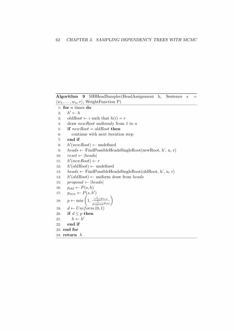
62 CHAPTER 3. SAMPLING DEPENDENCY TREES WITH MCMC
Algorithm 9 MHHeadSampler(HeadAssignment h, Sentence s =〈w1, . . . , wn, r〉, WeightFunction P)
1: for n times do2: h′ ← h3: oldRoot← i such that h(i) = r4: draw newRoot uniformly from 1 to n5: if newRoot = oldRoot then6: continue with next iteration step7: end if8: h′(newRoot)← undefined9: heads← FindPossibleHeadsSingleRoot(newRoot, h’, n, r)
10: reset← |heads|11: h′(newRoot)← r12: h′(oldRoot)← undefined13: heads← FindPossibleHeadsSingleRoot(oldRoot, h’, n, r)14: h′(oldRoot)← uniform draw from heads15: proposal← |heads|16: pold ← P (s, h)17: pnew ← P (s, h′)
18: p← min
(1,
1reset
pnew1
proposalpold
)19: d← Uniform (0, 1)20: if d ≤ p then21: h← h′
22: end if23: end for24: return h
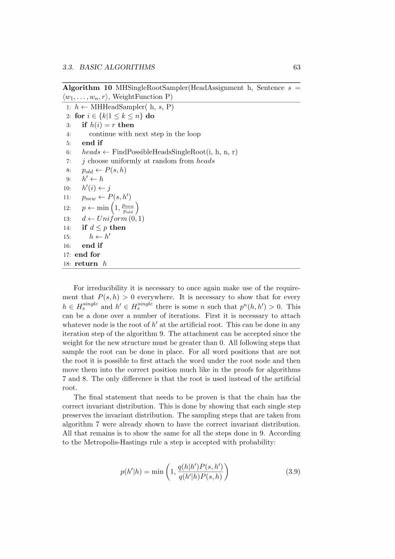
3.3. BASIC ALGORITHMS 63
Algorithm 10 MHSingleRootSampler(HeadAssignment h, Sentence s =〈w1, . . . , wn, r〉, WeightFunction P)
1: h← MHHeadSampler( h, s, P)2: for i ∈ {k|1 ≤ k ≤ n} do3: if h(i) = r then4: continue with next step in the loop5: end if6: heads← FindPossibleHeadsSingleRoot(i, h, n, r)7: j choose uniformly at random from heads8: pold ← P (s, h)9: h′ ← h
10: h′(i)← j11: pnew ← P (s, h′)
12: p← min(
1, pnew
pold
)13: d← Uniform (0, 1)14: if d ≤ p then15: h← h′
16: end if17: end for18: return h
For irreducibility it is necessary to once again make use of the require-ment that P (s, h) > 0 everywhere. It is necessary to show that for every
h ∈ Hsingles and h′ ∈ Hsingle
s there is some n such that pn(h, h′) > 0. Thiscan be a done over a number of iterations. First it is necessary to attachwhatever node is the root of h′ at the artificial root. This can be done in anyiteration step of the algorithm 9. The attachment can be accepted since theweight for the new structure must be greater than 0. All following steps thatsample the root can be done in place. For all word positions that are notthe root it is possible to first attach the word under the root node and thenmove them into the correct position much like in the proofs for algorithms7 and 8. The only difference is that the root is used instead of the artificialroot.
The final statement that needs to be proven is that the chain has thecorrect invariant distribution. This is done by showing that each single steppreserves the invariant distribution. The sampling steps that are taken fromalgorithm 7 were already shown to have the correct invariant distribution.All that remains is to show the same for all the steps done in 9. Accordingto the Metropolis-Hastings rule a step is accepted with probability:
p(h′|h) = min
(1,q(h|h′)P (s, h′)
q(h′|h)P (s, h)
)(3.9)

64 CHAPTER 3. SAMPLING DEPENDENCY TREES WITH MCMC
The proposal q(h|h′) is made in two steps. First a new head candidateis picked. The probability of being picked is 1
n for every root candidate withn the length of the sentence. Then A new position for the old root node ischosen from the children of the new root node. Represent the set of thesechildren as ch
′then this adds another term 1
|ch′ | due to the uniform choice.
This means that the Metropolis-Hastings rule becomes:
p(h′|h) = min
1,
1n|ch|P (h′)
1n|ch′ |P (h)
(3.10)
= min
1,
1|ch|P (h′)
1|ch′ |P (h)
(3.11)
This is exactly the acceptance probability used in algorithm 10. Theinvariance distribution follows.
The procedure that algorithm 10 uses to sample heads has the sameissues that algorithm 7 has. The movement of the algorithm through thespace of possible assignments can take a very long time even if it is not stuckin a local optimum. It would be desirable to have a sampler that exploresthe space of possible assignments more thoroughly in each iteration. Thisis done by attempting to move every possible word into the root positionand calculating the weight of each possible move for the old root. ThisAlgorithm has a simple problem. Assume that there is an iteration over thenodes 1, 2, . . . and node x is proposed as a new root. In other words thiswould mean that the probability of proposing x as root in this step is 1 andproposing a different root in the step is impossible. This would mean thatthe ratio:
q(h|h′)P (s, h′)
q(h′|h)P (s, h)(3.12)
would always be 0 if h, the old assignment, does not have x as a root.This means that the iteration over possible root candidates needs to beextended in such a way that it is possible to have a “reverse” step. This canbe done by adding the stipulation that a random word is proposed as rootif the current root node is equal to the node that would normally proposedas root. Algorithm 11 describes the sampling of the root with a Gibbslike approach. The iteration in line 1 would only ever propose the currentiteration number as root if it were not for the random step in line 6.
The main idea of algorithm 11 is comparatively simple. The algorithmiterates over all words and proposes them as the root of the sentence. As

3.3. BASIC ALGORITHMS 65
Algorithm 11 GibbsHeadSampler(HeadAssignment h, Sentence s =〈w1, . . . , wn, r〉, WeightFunction P, InPlaceProbability ip)
1: for 1 ≤ i ≤ n do2: if uniform draw from (0, 1) < ip then3: continue with next iteration step4: end if5: if h(i) = r then6: newRoot← uniform draw from 1, . . . , n7: p← 1
1n
8: else9: newRoot← i
10: p← 1n
11: end if12: if h(newRoot) = r then13: continue with next iteration step14: end if15: heads← FindPossibleHeadsSingleRoot(newRoot, h, n, r)16: h′ ← h17: reverseSum← 018: for head ∈ heads do19: h′(newRoot)← head20: reverseSum← reverseSum+ P (s, h′)21: end for22: h′(newRoot)← r23: h′(oldRoot)← undefined24: heads← FindPossibleHeadsSingleRoot(oldRoot, h, n, r)25: proposalSum← 026: for head ∈ heads do27: h′(oldRoot)← head28: proposalSum← proposalSum+ P (s, h′)29: q ← P (s, h′)30: end for31: h′(oldRoot)← drawn proportional to q
32: p← p1
reverseSum1
proposalSum
33: d← uniform draw from (0, 1)34: if d ≤ p then35: h← h′
36: end if37: end for38: return h
66 CHAPTER 3. SAMPLING DEPENDENCY TREES WITH MCMC
stated before, the possibility of a reverse step is given since different can-didate is proposed when the word is already in the root position. Once anew root candidate has been chosen, it is then necessary to sample a posi-tion into which the old root can be moved. This is again done in a moresystematic fashion than in the sampler given by algorithm 9. The weight ofeach possible move for the old root is calculated and then a draw propor-tional to these weights is made. This extended MCMC scheme allows formore informed moves in each iteration but it requires some more resourcesthan the uniform approach. The head sampling step described by algorithm11 takes function evaluations in the order of O(n2). Here n is again thelength of the sentence in question. This is the case since there are n headcandidates and it is possible that the calculation of the proposal function isrepeated a number of steps bounded by n. The sampler also has to computethe movement options for the new root candidate. This is the case sincethe Metropolis-Hastings rule requires correct computations of the likelihoodof a reverse step and this reverse step would entail moving around the newroot candidate. It is necessary to make a remark on the skipping step inline 2. This was added in order to enable an easy proof of the correctness ofthe sampler. In practice it is possible to choose the in place step probabilitythat is used here rather small. The value used throughout this thesis is 1
1000 .This means that any skipping is done rarely. The function of the skipping isto allow for in place steps. These will be necessary to allow for the proof ofirreducibility and aperiodicity. In practical applications there will be someroot assignment that will be better than all other choices. This leads toin place steps without any use of the in place probability. This is anotherreason why it is not necessary to make this skipping very likely.
Algorithm 12 puts the Gibbs sampler for general positions together withthe Gibbs style sampling of root nodes. The umber of weight functionevaluations of the algorithm is still in O(n2). This is the same class as theoriginal algorithm 8. The algorithm still only uses linear memory. Thissection will conclude with the proof that the given algorithm can indeed beused to construct a correct sampler.
Lemma 6 (Correctness of Algorithm 12). Let s be a sentence and P bea weight function that assigns weight to the combination of the sentenceand and any head assignment function h ∈ Hsingle
s . It is Assumed thatfor any head function h ∈ Hsingle
s it is true that P (s, h) > 0. Construct a
Markov Chain M = 〈Hsingles , p〉. Here p(h, h′) is equal to the probability that
algorithm 12 returns h′ when given h, s, P and some small value of ip asinput. M is irreducible, aperiodic and has an invariant distribution equal toP (s, h) for any head assignment h ∈ Hsingle
s .
Proof. The first step is again the proof of the aperiodicity. The main part ofthe sampler is the same as that of the Gibbs sampler described by algorithm8 and the reasoning why in place steps are possible here is the same as in the
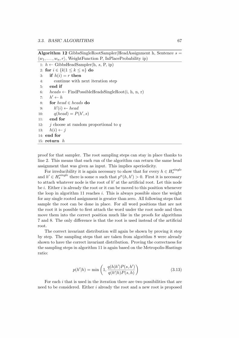
3.3. BASIC ALGORITHMS 67
Algorithm 12 GibbsSingleRootSampler(HeadAssignment h, Sentence s =〈w1, . . . , wn, r〉, WeightFunction P, InPlaceProbability ip)
1: h← GibbsHeadSampler(h, s, P, ip)2: for i ∈ {k|1 ≤ k ≤ n} do3: if h(i) = r then4: continue with next iteration step5: end if6: heads← FindPossibleHeadsSingleRoot(i, h, n, r)7: h′ ← h8: for head ∈ heads do9: h′(i)← head
10: q(head) = P (h′, s)11: end for12: j choose at random proportional to q13: h(i)← j14: end for15: return h
proof for that sampler. The root sampling steps can stay in place thanks toline 2. This means that each run of the algorithm can return the same headassignment that was given as input. This implies aperiodicity.
For irreducibility it is again necessary to show that for every h ∈ Hsingles
and h′ ∈ Hsingles there is some n such that pn(h, h′) > 0. First it is necessary
to attach whatever node is the root of h′ at the artificial root. Let this nodebe i. Either i is already the root or it can be moved to this position wheneverthe loop in algorithm 11 reaches i. This is always possible since the weightfor any single rooted assignment is greater than zero. All following steps thatsample the root can be done in place. For all word positions that are notthe root it is possible to first attach the word under the root node and thenmove them into the correct position much like in the proofs for algorithms7 and 8. The only difference is that the root is used instead of the artificialroot.
The correct invariant distribution will again be shown by proving it stepby step. The sampling steps that are taken from algorithm 8 were alreadyshown to have the correct invariant distribution. Proving the correctness forthe sampling steps in algorithm 11 is again based on the Metropolis-Hastingsratio:
p(h′|h) = min
(1,q(h|h′)P (s, h′)
q(h′|h)P (s, h)
)(3.13)
For each i that is used in the iteration there are two possibilities that areneed to be considered. Either i already the root and a new root is proposed
68 CHAPTER 3. SAMPLING DEPENDENCY TREES WITH MCMC
or i will be proposed as the root. The case in which i is the root and is alsoproposed7 can be ignored since the ratio above is always fulfilled for a stepthat is made in place. In both discussed cases it is necessary to consider theproposal distribution q for both the case in which a random node is proposedand the case in which the fixed node is chosen. This is the case since boththe proposal likelihood and the likelihood for the reverse proposal appear inthe ratio. When a random candidate is chosen the chance of any word beingchosen is 1
n where n is the length of the sentence. This factor changes to 1if i is proposed. This portion of the ratio will be denoted by qnew. The nextstep in the construction of the proposal is choosing a head for the old root,
this head is chosen according to P (s,h′)Z and the same would be true for the
reverse step that would chose the old assignment for the new root accordingto P (s,h)
Z′ . Note that Z 6= Z ′. This leads to the Metropolis-Hastings rule:
p(h′|h) = min
(1, qnew
P (s,h)Z′ P (s, h′)
P (s,h′)Z P (s, h)
)(3.14)
= min
(1, qnew
1Z′
1Z
)(3.15)
This is the ratio used by the root sampling in each step.
The two samplers presented in this section introduce some additionalcomplication to the sampling process in order to deal with the constraint ofhaving only a single root node. In the next section it is shown that it is mucheasier to deal with the projective constraint. The algorithms presented sofar could all be applied successfully in this scenario. At the same time itis interesting to exploit the interaction of the single root and the projectiveconstraint. This will also be investigated in this thesis.
3.3.4 Sampling with the Projective Constraint
The first part of this section deals with showing that the techniques devel-oped for the sampling of general dependency trees are also applicable forprojective dependency trees. Afterwards some additional work is presentedthat shows how the constraint to projective structures can be combined withthe single root constraint. This latter section tries to exploit the fact thatthere are only a few new roots that can be chosen without violating thesingle root constraint. This brings up one of the most important differencesbetween sampling with the projective structures and unconstrained depen-dency trees. There are generally far less possible head assignments that
7Which in the given algorithm means that one step is skipped.
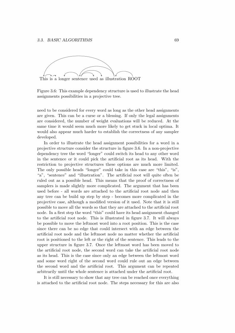
3.3. BASIC ALGORITHMS 69
This is a longer sentence used as illustration ROOT
Figure 3.6: This example dependency structure is used to illustrate the headassignments possibilities in a projective tree.
need to be considered for every word as long as the other head assignmentsare given. This can be a curse or a blessing. If only the legal assignmentsare considered, the number of weight evaluations will be reduced. At thesame time it would seem much more likely to get stuck in local optima. Itwould also appear much harder to establish the correctness of any samplerdeveloped.
In order to illustrate the head assignment possibilities for a word in aprojective structure consider the structure in figure 3.6. In a non-projectivedependency tree the word “longer” could switch its head to any other wordin the sentence or it could pick the artificial root as its head. With therestriction to projective structures these options are much more limited.The only possible heads “longer” could take in this case are “this”, “is”,“a”, “sentence” and “illustration”. The artificial root will quite often beruled out as a possible head. This means that the proof of correctness ofsamplers is made slightly more complicated. The argument that has beenused before - all words are attached to the artificial root node and thenany tree can be build up step by step - becomes more complicated in theprojective case, although a modified version of it used. Note that it is stillpossible to move all the words so that they are attached to the artificial rootnode. In a first step the word “this” could have its head assignment changedto the artificial root node. This is illustrated in figure 3.7. It will alwaysbe possible to move the leftmost word into a root position. This is the casesince there can be no edge that could intersect with an edge between theartificial root node and the leftmost node no matter whether the artificialroot is positioned to the left or the right of the sentence. This leads to theupper structure in figure 3.7. Once the leftmost word has been moved tothe artificial root node, the second word can take the artificial root nodeas its head. This is the case since only an edge between the leftmost wordand some word right of the second word could rule out an edge betweenthe second word and the artificial root. This argument can be repeatedarbitrarily until the whole sentence is attached under the artificial root.
It is still necessary to show that any tree can be reached once everythingis attached to the artificial root node. The steps necessary for this are also
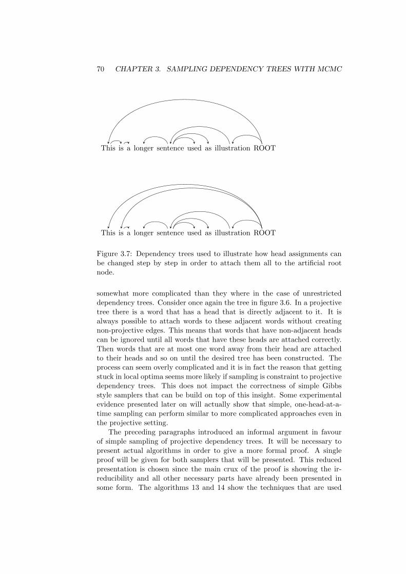
70 CHAPTER 3. SAMPLING DEPENDENCY TREES WITH MCMC
This is a longer sentence used as illustration ROOT
This is a longer sentence used as illustration ROOT
Figure 3.7: Dependency trees used to illustrate how head assignments canbe changed step by step in order to attach them all to the artificial rootnode.
somewhat more complicated than they where in the case of unrestricteddependency trees. Consider once again the tree in figure 3.6. In a projectivetree there is a word that has a head that is directly adjacent to it. It isalways possible to attach words to these adjacent words without creatingnon-projective edges. This means that words that have non-adjacent headscan be ignored until all words that have these heads are attached correctly.Then words that are at most one word away from their head are attachedto their heads and so on until the desired tree has been constructed. Theprocess can seem overly complicated and it is in fact the reason that gettingstuck in local optima seems more likely if sampling is constraint to projectivedependency trees. This does not impact the correctness of simple Gibbsstyle samplers that can be build on top of this insight. Some experimentalevidence presented later on will actually show that simple, one-head-at-a-time sampling can perform similar to more complicated approaches even inthe projective setting.
The preceding paragraphs introduced an informal argument in favourof simple sampling of projective dependency trees. It will be necessary topresent actual algorithms in order to give a more formal proof. A singleproof will be given for both samplers that will be presented. This reducedpresentation is chosen since the main crux of the proof is showing the ir-reducibility and all other necessary parts have already been presented insome form. The algorithms 13 and 14 show the techniques that are used

3.3. BASIC ALGORITHMS 71
to sample projective dependency trees. The reader will immediately noticethat the presented algorithms are virtually identical to the algorithms 7 and8. The only difference for algorithm 13 is found in line 2. Algorithm 14differs in line 2. The difference for both algorithms is the fact that onlyedges that do not violate the projective tree constraint are considered. Thenext lemma shows that both these algorithms are correct samplers as longas all projective trees are assigned weight greater than 0.
Algorithm 13 MHProjectiveSampler(HeadAssignment h, Sentence s =〈w1, . . . , wn, r〉, WeightFunction P)
1: for i ∈ {k|1 ≤ k ≤ n} do2: heads← FindProjectiveHeadCandidates(i, h, n, r)3: j choose uniformly at random from heads4: pold ← P (s, h)5: h′ ← h6: h′(i)← j7: pnew ← P (s, h′)
8: p← min(
1, pnew
pold
)9: d← Uniform (0, 1)
10: if d ≤ p then11: h← h′
12: end if13: end for14: return h
Algorithm 14 GibbsProjectiveSampler(HeadAssignment h, Sentence s =〈w1, . . . , wn, r〉, WeightFunction P)
1: for i ∈ {k|1 ≤ k ≤ n} do2: heads← FindProjectiveHeadCandidates(i, h, n, r)3: h′ ← h4: for head ∈ heads do5: h′(i)← head6: q(head) = P (s, h′)7: end for8: j choose at random proportional to q9: h(i)← j
10: end for11: return h
Lemma 7 (Correctness of Algorithm 13 and 2). Let s be a sentence and Pbe a weight function that assigns weight to the combination of the sentenceand and any head assignment function h ∈ Hprojective
s . It is assumed that
72 CHAPTER 3. SAMPLING DEPENDENCY TREES WITH MCMC
for any head assignment function h ∈ Hprojectives it is true that P (s, h) > 0.
Construct a Markov Chain M = 〈Hprojectives , p〉. Here p(h, h′) is equal to the
probability that algorithm 13 returns h′ when given h, s and P as input. Mis irreducible, aperiodic and has an invariant distribution equal to P (s, h)for any head assignment function h ∈ Hprojective
s . The same is true if pis replaced by p′ and p′(h, h′) is equal to the probability that algorithm 14returns h′ when given h, s and P as input.
Proof. The proofs for lemmas 3 and 4 can be consulted in order to see thatthe samplers can stay in place for every word they sample. This ensuresaperiodicity. The same proofs also contain the necessary considerations toshow that both algorithms lead to the correct invariant distribution. Itremains to be shown that the sampler does indeed allow moves from everypossible head assignment to every other possible head assignment.
As mentioned before, if the word positions 0, . . . ,m are already attachedto the artificial root, then it is possible to attach the word number m + 1without creating a non-projective tree. If the artificial root node is placedto the left of the sentence, then the an edge that would cross with the edgebetween the artificial root node and m + 1 would have to be between oneof the positions 0, . . . ,m and some word right of word number m+ 1. Thisedge can not exist because of the pre-supposition. If the artificial node isplaced to the right of the sentence, then a crossing is still impossible forthe same reason. In order to move to any tree it is therefore possible tomove every word to be attached to the artificial root. Basically there are noexternal-edges for the artificial root so removing cover-edges makes sure thatattachment as a root is allowed. Once every word is attached at the artificialroot, it is possible to generate every head assignment h′ by first attachingevery word that is attached to one of its direct neighbours in h′. Everyword without such an attachment is sampled without making any change.There can be no crossing edges with these attachments. This process is thenrepeated for all distances greater than adjacent. Once words in distance kfrom their heads in h′ have been attached correctly, it is then possible toattach words in distance k + 1 correctly. This is the case since if there isan edge between the words w and w′ in h′, then all words between themare attached to a word between w and w′ or w and w′ themselves. Becauseall positions in between are closer to the to their selected heads then w andw′ are to each other, they have already been attached. This means thatthere are no crossing edges preventing the attachment of the two words.This shows that is is possible to generate the desired head assignments inno more steps that one plus the length of the longest desired edge. All thedescribed steps are possible since the the weight function is greater thanzero everywhere.
3.3. BASIC ALGORITHMS 73
Sampling Projective, Single Rooted Dependency Trees
In this section the existing approaches are extended to combine the restric-tions. It would be possible to use the different samplers developed for thesingle rooted setting in a projective context. This could simply be doneby setting the weight for all trees that do not conform to the additionalrestriction to 0. This would once again lead to a large number of wastedcomputations. Instead an alternative approach will be considered.
In the first tree in figure 3.8 it would be possible to move the leftmostdirect child of “cleaned” into the root position and make “cleaned” its right-most child. This would generate the second tree in figure 3.8. Note that thismove always keeps dependency structures projective. The edge between theold root node o and the new root node n is reversed. The new edge betweenthe artificial root node and n does not cross with any other edge since therehas been no crossing edge for the connection o and the artificial root nodeand there is also none for the connection between o and n. Any edge thatwould cross with the new edge would have to connect a word outside of thiscombined span with a word inside of it. This would already have lead to acrossing edge.
A very similar move could be made with the rightmost child of “cleaned”.Making “bathroom” the root of the sentence and attaching “cleaned” as itsleftmost child. This would create the third tree in figure 3.8. The argumentthat shows that this operation does not create any non-projective edges isessentially the same as the one presented for the other direction. Any of thetwo operations can be reversed by applying the other one immediately af-terwards. This means that they can be very easily used to prove correctnessby using the Metropolis-Hastings rule.
Algorithm 15 HeadCandidateGenerator(HeadAssignment h, Sentence s =〈w1, . . . , wn, r〉)
1: oldRoot← i such that h(i) = r2: candidates← {}3: if ∃i ∈ 1, . . . , n : h(i) = oldRoot ∧ i < oldRoot then4: candidates← candidates ∪ {mini∈1,...,n ({i|h(i) = oldRoot})}5: end if6: if ∃i ∈ 1, . . . , n : h(i) = oldRoot ∧ i > oldRoot then7: candidates← candidates ∪ {maxi∈1,...,n ({i|h(i) = oldRoot})}8: end if9: return candidates
From the described operations it is possible to construct a sampler for theroot node. Algorithm 16 describes this sampler. It takes some considerationin order to see that this operation is actually sufficient in order to reachany possible tree. Recall the proof for lemma 7. It is possible to create any

74 CHAPTER 3. SAMPLING DEPENDENCY TREES WITH MCMC
The janitor cleaned the dirty bathroom ROOT
The janitor cleaned the dirty bathroom ROOT
The janitor cleaned the dirty bathroom ROOT
Figure 3.8: A simple example sentence used to illustrate the single rootsampling operation for projective dependency trees.
Algorithm 16 ProjectiveRootSampler(HeadAssignment h, Sentence s =〈w1, . . . , wn, r〉, WeightFunction P)
1: k ← 02: while k < 2 do3: oldRoot← i such that h(i) = r4: candidates← HeadCandidateGenerator(h, s)5: newRoot← uniform draw from candidates6: h′ ← h7: h′(newRoot)← r8: h′(oldRoot)← newRoot9: candidates′ ← HeadCandidateGenerator(h’, s)
10: p← min
(1,
1candidates′ P (s,h′)
1candidates
P (s,h)
)11: d← Uniform (0, 1)12: if d ≤ p then13: h← h′
14: end if15: k ← k + 116: end while17: return h
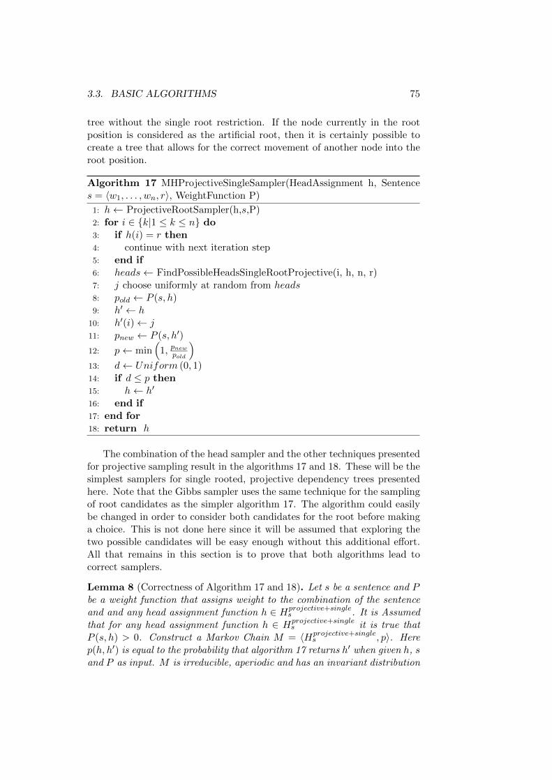
3.3. BASIC ALGORITHMS 75
tree without the single root restriction. If the node currently in the rootposition is considered as the artificial root, then it is certainly possible tocreate a tree that allows for the correct movement of another node into theroot position.
Algorithm 17 MHProjectiveSingleSampler(HeadAssignment h, Sentences = 〈w1, . . . , wn, r〉, WeightFunction P)
1: h← ProjectiveRootSampler(h,s,P)2: for i ∈ {k|1 ≤ k ≤ n} do3: if h(i) = r then4: continue with next iteration step5: end if6: heads← FindPossibleHeadsSingleRootProjective(i, h, n, r)7: j choose uniformly at random from heads8: pold ← P (s, h)9: h′ ← h
10: h′(i)← j11: pnew ← P (s, h′)
12: p← min(
1, pnew
pold
)13: d← Uniform (0, 1)14: if d ≤ p then15: h← h′
16: end if17: end for18: return h
The combination of the head sampler and the other techniques presentedfor projective sampling result in the algorithms 17 and 18. These will be thesimplest samplers for single rooted, projective dependency trees presentedhere. Note that the Gibbs sampler uses the same technique for the samplingof root candidates as the simpler algorithm 17. The algorithm could easilybe changed in order to consider both candidates for the root before makinga choice. This is not done here since it will be assumed that exploring thetwo possible candidates will be easy enough without this additional effort.All that remains in this section is to prove that both algorithms lead tocorrect samplers.
Lemma 8 (Correctness of Algorithm 17 and 18). Let s be a sentence and Pbe a weight function that assigns weight to the combination of the sentenceand and any head assignment function h ∈ Hprojective+single
s . It is Assumedthat for any head assignment function h ∈ Hprojective+single
s it is true thatP (s, h) > 0. Construct a Markov Chain M = 〈Hprojective+single
s , p〉. Herep(h, h′) is equal to the probability that algorithm 17 returns h′ when given h, sand P as input. M is irreducible, aperiodic and has an invariant distribution
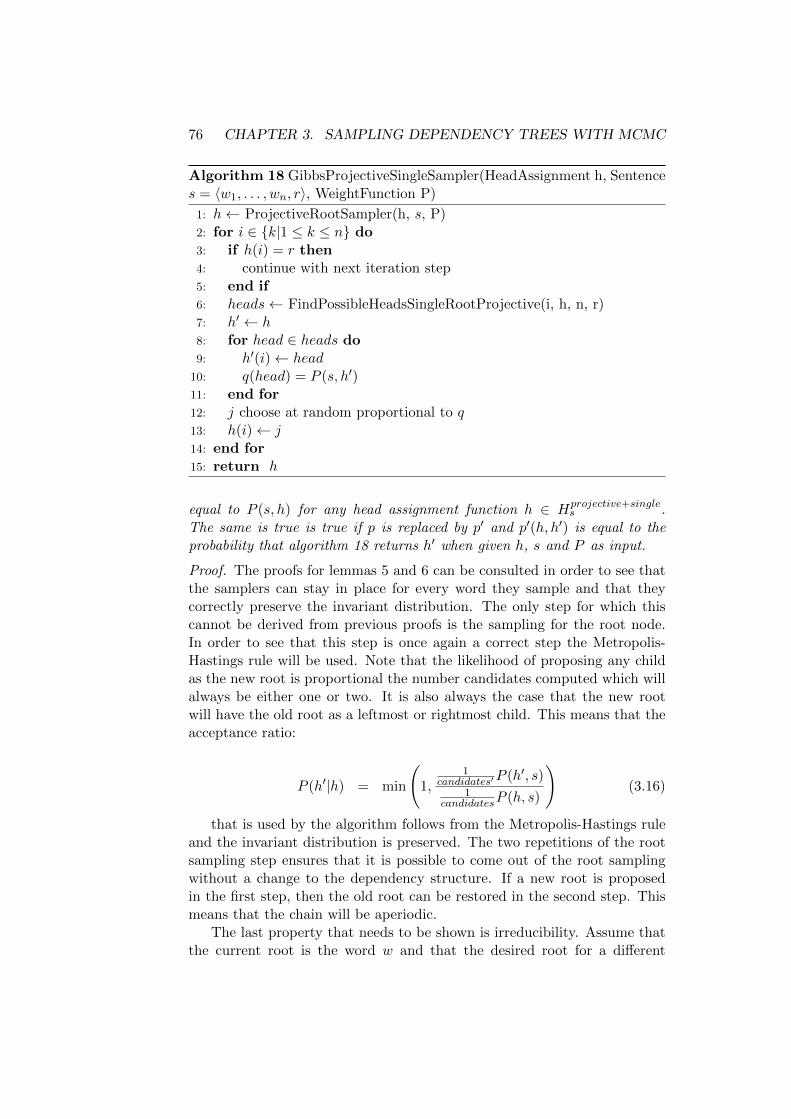
76 CHAPTER 3. SAMPLING DEPENDENCY TREES WITH MCMC
Algorithm 18 GibbsProjectiveSingleSampler(HeadAssignment h, Sentences = 〈w1, . . . , wn, r〉, WeightFunction P)
1: h← ProjectiveRootSampler(h, s, P)2: for i ∈ {k|1 ≤ k ≤ n} do3: if h(i) = r then4: continue with next iteration step5: end if6: heads← FindPossibleHeadsSingleRootProjective(i, h, n, r)7: h′ ← h8: for head ∈ heads do9: h′(i)← head
10: q(head) = P (s, h′)11: end for12: j choose at random proportional to q13: h(i)← j14: end for15: return h
equal to P (s, h) for any head assignment function h ∈ Hprojective+singles .
The same is true is true if p is replaced by p′ and p′(h, h′) is equal to theprobability that algorithm 18 returns h′ when given h, s and P as input.
Proof. The proofs for lemmas 5 and 6 can be consulted in order to see thatthe samplers can stay in place for every word they sample and that theycorrectly preserve the invariant distribution. The only step for which thiscannot be derived from previous proofs is the sampling for the root node.In order to see that this step is once again a correct step the Metropolis-Hastings rule will be used. Note that the likelihood of proposing any childas the new root is proportional the number candidates computed which willalways be either one or two. It is also always the case that the new rootwill have the old root as a leftmost or rightmost child. This means that theacceptance ratio:
P (h′|h) = min
(1,
1candidates′P (h′, s)
1candidatesP (h, s)
)(3.16)
that is used by the algorithm follows from the Metropolis-Hastings ruleand the invariant distribution is preserved. The two repetitions of the rootsampling step ensures that it is possible to come out of the root samplingwithout a change to the dependency structure. If a new root is proposedin the first step, then the old root can be restored in the second step. Thismeans that the chain will be aperiodic.
The last property that needs to be shown is irreducibility. Assume thatthe current root is the word w and that the desired root for a different
3.4. SAMPLING WITH GLOBAL CHANGES 77
head assignment that is to be reached is w′ 6= w. Use the argument forirreducibility that has been used in the proof of lemma 7 to show that anytree with root w can be reached by the steps not sampling the root, thenthere is certainly such tree that has w′ as the leftmost or rightmost child ofw. This means that w′ can be moved into the root position. Once that isdone, the techniques from lemma 7 can also be used to show that any treewith root w′ can be reached by using w′ instead of the artificial root. Asargued before, the necessary in place steps that keep the root w′ are possibledue to the repetition of the root sampling. Each configuration that is neededin this process has weight greater 0 as a result of the pre-suppositions of thelemma.
The last lemma concludes the considerations be given to the problem ofsampling dependency structures with simple, one word at a time approaches.All the algorithms presented are provably correct for their respective prob-lems. At the same time it would be desirable to be able to make more globalsampling moves in order to be able to move out of local optima. Approachesto the reconstruction of the complete dependency tree are given in the nextsection.
3.4 Sampling with Global Changes
This section presents two algorithms that extend the previous samplers byadding a step that changes most of the tree in a single step. Essentially acompletely new tree is proposed and then either accepted or rejected accord-ing to the Metropolis-Hastings rule. In order to implement this efficientlytwo things will be necessary. One requirement is the ability to compute theprobability with which a tree will be proposed. Computing this value maybe somewhat more difficult than doing the same for the “single word at atime” samplers that have been presented so far. The second requirement isthat the proposal distribution is “well suited” to sampling from the desireddistribution. The simplest way to define well suited would be to have it de-note a distribution that is equal to the distribution that is sampled. Anotherway to define the same concept would be to take some measure of distancebetween probability distributions such as the Kullback–Leibler divergence[6] and looking for distribution that has a small distance according to thatmeasure. Since the only reason an MCMC approach is used in the first placeis that fact that the desired distribution is very hard to sample from directly,it would seem that working with any “well suited” distribution according tothe two criteria just mentioned is completely infeasible. The actual distri-butions used will mostly be left up to any user of the algorithms, with therestriction that the first algorithm needs the weights to factor along edges.
The first algorithm that presented is based on the fact that it is generallycomputationally feasible to sample random trees when the likelihood of each
78 CHAPTER 3. SAMPLING DEPENDENCY TREES WITH MCMC
trees factors along the edges. This could be done with projective trees8
[32, 115, 68] but here an investigation will be made into solving this problemfor general dependency trees. In this context it is possible to make use ofexisting research into the sampling of directed spanning trees for graphs[11, 117, 23].
The second algorithm given here is based on constructing the proposedtree step by step and using the information available so far in order tocreate a better proposal. This way of sampling the structures could easilybe applied to other structures. It is also a generalization of existing otherapproaches to sampling such as the ones based on constructing charts inorder to produce a proposal [56]. One of the very useful properties of thissampler is the fact that is no longer requires the weight function to be definedeverywhere. This would theoretically allow for the handling of arbitrary hardconstraints. The sampling process could actually benefit from additionalhard constraints because they reduce the number of trees that would haveto be considered.
Both approaches can and will be combined with other sampling ap-proaches. Proving the correctness of these approaches is generally muchsimpler than it has been for the other samplers. This is mainly the casesince the global sampling steps makes showing irreducibility trivial and ape-riodicity will generally follow from the chance that the sampler reproducesthe same tree. This can actually happen with some frequency if a configura-tion with high weight has been reached and the proposal distribution tendsto match the weight function well.
The next section will explain how existing research into the samplingof random spanning trees can be applied to arbitrary distributions overdependency trees through the use of MCMC. After this the greedy approachis elaborated on.
3.4.1 Sampling from a Factored Distribution
Assume that there is a finite set N . In the applications relevant to thisthesis this set will be the positions for words in a sentence. Assume thatthere is a function w : N ×N → R+ from pairs of elements in N to positivereal numbers. The pair 〈N,w〉 is then a directed graph [51]. If w(a, b) = 0then this is taken to mean that the edge 〈a, b〉 is not in the graph. Sincedependency trees can be interpreted as graphs there is a direct connectionbetween problems concerning graphs and problems concerning dependencytrees. One graph theoretical problem is the generation of random, spanningarborescences from a graph according to its weights. A spanning graph for〈N,w〉 is another graph 〈N,w′〉 such that for any two elements 〈vi, vi+1〉of N it is true that: w′(vi, vi+1) = 0 ∨ w′(vi, vi+1) = w(vi, vi+1). For any
8Even though the constraint to projective trees removes the factorization along edges,because prohibiting crossing edges means edges are dependent on each other.
3.4. SAMPLING WITH GLOBAL CHANGES 79
pair is must also be true that the two elements can be connected through asequence of other v′ ∈ N . For this sequence it must hold that any successivepair 〈vi, vi+1〉 of elements in it has w′(vi, vi+1) > 0 ∨ w′(vi+1, vi) > 0. Anarborescence is an extension of this concept. There is a single element thatcan be reached by some sequence from any other element in N . The require-ment on the weights is extended so that any adjacent elements 〈vi, vi+1〉 inthe sequences must conform to w′(vi, vi+1) > 0. It must also be true thatthere is no such sequence that connects any node with itself. The readerwill quickly notice that this structure corresponds to a dependency tree ifthe elements in N are the word positions in a sentence. If an arborescencea is generate from a graph then this means that the probability of beingproduced is proportional to the multiplication of the weights in a. In otherwords the probability Pa of generating any arborescence is given by:
Pa(a = 〈N,w′〉) =
∏〈vi,vi+1〉∈N×N w′(vi, vi+1)
Z(3.17)
In the given formula the value Z is a normalizer that ensures that thedifferent values sum to one.
Since there is a correspondence between these arborescence and depen-dency trees the task of generating the former randomly can be used forsampling dependency trees. If the weight function used in sampling fac-tors according to the edges, then any techniques for sampling arborescencescan be used directly. In any other setting it will be possible to use thesetechniques to propose a new tree and then accept or reject the proposalaccording to the Metropolis-Hastings rule:
p(h′|h) =Pa(s, h)P (s, h′)
Pa(s, h′)P (s, h)(3.18)
In order to apply these techniques it is necessary to approximate theweight of any dependency tree by some auxiliary distribution that factorsalong edges.
There are two general types of approaches used to solve the problemof random generation of arborescences. The first type is based on exactlycalculating the sum of the weight of all possible arborescences. This can bedone by using the Matrix Tree Theorem [23]. The simplest way to generate anew proposal in this way would be to iterated over the different words. Theweight of the arborescences that still remain after choosing a certain head iscomputed and a proportional draw is made. This approach can be made torequire significantly less computation by re-using intermediate results [23].The second type of technique is based on random walks on the graph. Suchalgorithms generally have no guaranteed upper bounds on their worst caseruntime and depending on the structure of the underlying graph even the
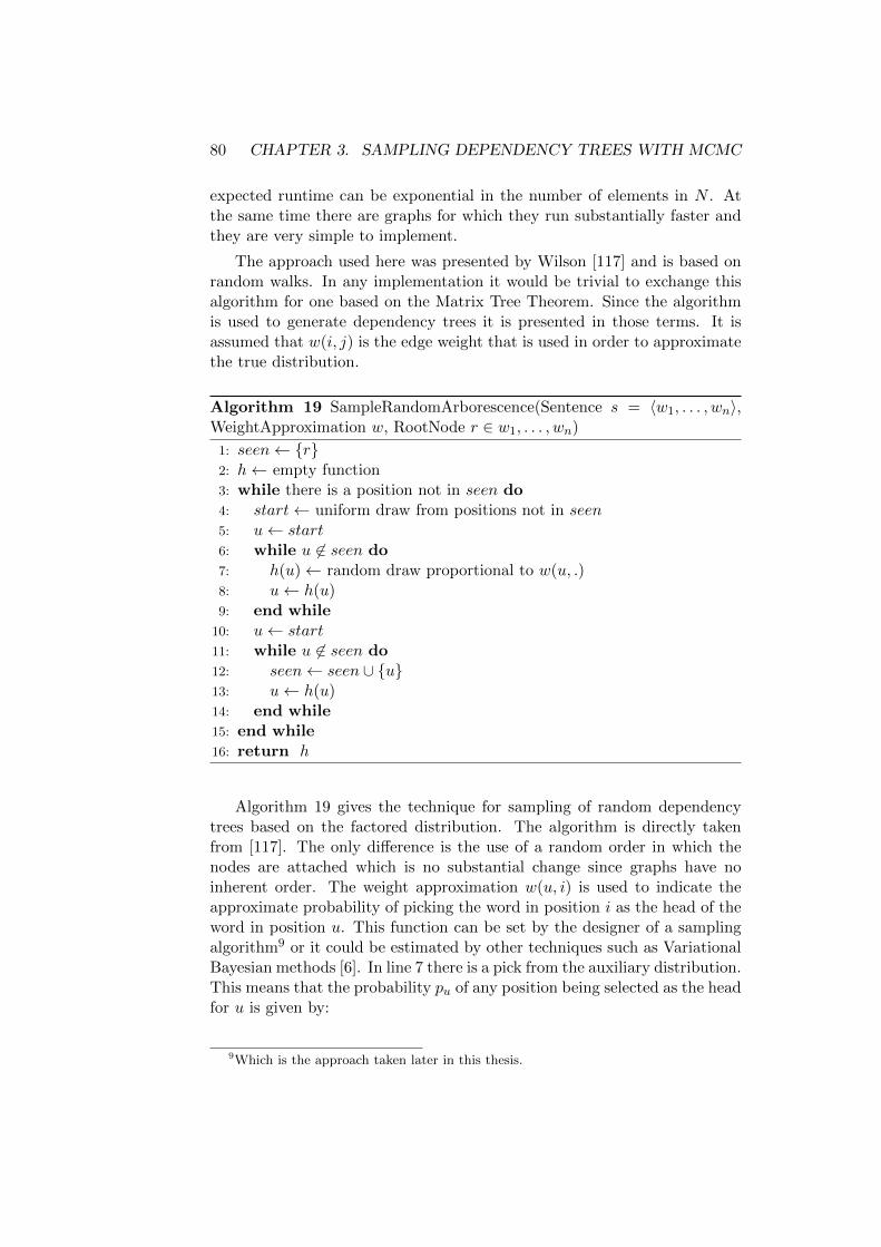
80 CHAPTER 3. SAMPLING DEPENDENCY TREES WITH MCMC
expected runtime can be exponential in the number of elements in N . Atthe same time there are graphs for which they run substantially faster andthey are very simple to implement.
The approach used here was presented by Wilson [117] and is based onrandom walks. In any implementation it would be trivial to exchange thisalgorithm for one based on the Matrix Tree Theorem. Since the algorithmis used to generate dependency trees it is presented in those terms. It isassumed that w(i, j) is the edge weight that is used in order to approximatethe true distribution.
Algorithm 19 SampleRandomArborescence(Sentence s = 〈w1, . . . , wn〉,WeightApproximation w, RootNode r ∈ w1, . . . , wn)
1: seen← {r}2: h← empty function3: while there is a position not in seen do4: start← uniform draw from positions not in seen5: u← start6: while u 6∈ seen do7: h(u)← random draw proportional to w(u, .)8: u← h(u)9: end while
10: u← start11: while u 6∈ seen do12: seen← seen ∪ {u}13: u← h(u)14: end while15: end while16: return h
Algorithm 19 gives the technique for sampling of random dependencytrees based on the factored distribution. The algorithm is directly takenfrom [117]. The only difference is the use of a random order in which thenodes are attached which is no substantial change since graphs have noinherent order. The weight approximation w(u, i) is used to indicate theapproximate probability of picking the word in position i as the head of theword in position u. This function can be set by the designer of a samplingalgorithm9 or it could be estimated by other techniques such as VariationalBayesian methods [6]. In line 7 there is a pick from the auxiliary distribution.This means that the probability pu of any position being selected as the headfor u is given by:
9Which is the approach taken later in this thesis.
3.4. SAMPLING WITH GLOBAL CHANGES 81
p(i) =w(u, i)∑
j∈1,...,nw(u, j)(3.19)
This once again shows that the probability of any tree being generate isonly dependent on single edge weights. The algorithm also requires that aroot is specified. It is generally assumed that a root node is given to initializethe algorithm. The root node is assumed to be part of the sentence. Itcould be the artificial root node attached at the end or the beginning of thesentence. The root could also be one of the regular words in the sentence.This will be useful when the single root restriction is used. In this case theartificial root node is ignored. The expected number of times it is necessaryto pick a new head is proportional to the expected commute time betweennodes. This and the fact that the probability of any tree being picked isproportional to:
∏〈vi,vi+1〉∈N×N w′(vi, vi+1)
Z(3.20)
is proven in the paper by Wilson [117]. While the algorithm will almostsurely10 stop at some point, it may run for a long time and the algorithmsbased on the Matrix Tree Theorem could be substituted for a predictablerunning time. As stated before the Wilson algorithm is chosen mainly forits very simple implementation.
It may not be immediately clear that the algorithm does indeed producea tree. An illustration of the way that the algorithm works is given in figure3.9. Note that the algorithm moves in the opposite direction of the arrows.In the first step a head is chosen for the word “ The”. Note that edges thatare not yet guaranteed to be part of the finished tree are marked by “new”while edges that are guaranteed to be in the tree are marked as “seen”.In the second step a loop is created. Note that in the next step the loopis broken since a new head is chosen for “The”. Each loop will eventuallybe broken11 since otherwise the algorithm would never move out of theloop. Since the word “cleaned” is no longer reachable from “The”, its headassignment will not be added. After the two first words have been added anew head is sampled for “cleaned”. The algorithm would then proceed inthe same manner for all remaining word positions.
Now that a technique for sampling edge factored trees has been pre-sented, the next natural step is extending this technique to a general MCMCsampler. The MCMC sampler presented as algorithm 20 accomplishes thisextension. Each run of the algorithm requires only two evaluations of the
10In the strict probability theoretic sense.11Under the condition that the algorithm terminates.

82 CHAPTER 3. SAMPLING DEPENDENCY TREES WITH MCMC
The janitor cleaned the dirty bathroom ROOT
new
The janitor cleaned the dirty bathroom ROOT
new
The janitor cleaned the dirty bathroom ROOT
new
new
The janitor cleaned the dirty bathroom ROOT
new
new
new
The janitor cleaned the dirty bathroom ROOT
seen new
seen
Figure 3.9: A sequence of dependency trees that illustrates how algorithm19 operates.
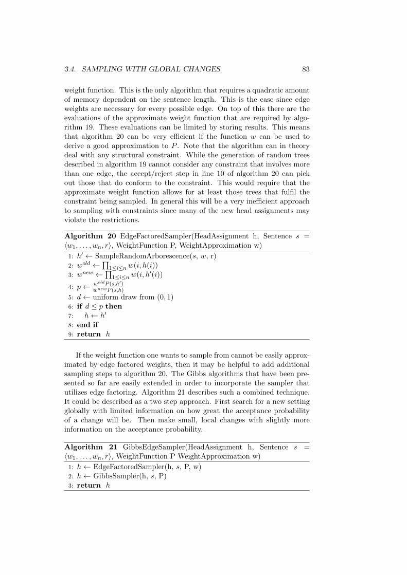
3.4. SAMPLING WITH GLOBAL CHANGES 83
weight function. This is the only algorithm that requires a quadratic amountof memory dependent on the sentence length. This is the case since edgeweights are necessary for every possible edge. On top of this there are theevaluations of the approximate weight function that are required by algo-rithm 19. These evaluations can be limited by storing results. This meansthat algorithm 20 can be very efficient if the function w can be used toderive a good approximation to P . Note that the algorithm can in theorydeal with any structural constraint. While the generation of random treesdescribed in algorithm 19 cannot consider any constraint that involves morethan one edge, the accept/reject step in line 10 of algorithm 20 can pickout those that do conform to the constraint. This would require that theapproximate weight function allows for at least those trees that fulfil theconstraint being sampled. In general this will be a very inefficient approachto sampling with constraints since many of the new head assignments mayviolate the restrictions.
Algorithm 20 EdgeFactoredSampler(HeadAssignment h, Sentence s =〈w1, . . . , wn, r〉, WeightFunction P, WeightApproximation w)
1: h′ ← SampleRandomArborescence(s, w, r)2: wold ←
∏1≤i≤nw(i, h(i))
3: wnew ←∏
1≤i≤nw(i, h′(i))
4: p← woldP (s,h′)wnewP (s,h)
5: d← uniform draw from (0, 1)6: if d ≤ p then7: h← h′
8: end if9: return h
If the weight function one wants to sample from cannot be easily approx-imated by edge factored weights, then it may be helpful to add additionalsampling steps to algorithm 20. The Gibbs algorithms that have been pre-sented so far are easily extended in order to incorporate the sampler thatutilizes edge factoring. Algorithm 21 describes such a combined technique.It could be described as a two step approach. First search for a new settingglobally with limited information on how great the acceptance probabilityof a change will be. Then make small, local changes with slightly moreinformation on the acceptance probability.
Algorithm 21 GibbsEdgeSampler(HeadAssignment h, Sentence s =〈w1, . . . , wn, r〉, WeightFunction P WeightApproximation w)
1: h← EdgeFactoredSampler(h, s, P, w)2: h← GibbsSampler(h, s, P)3: return h
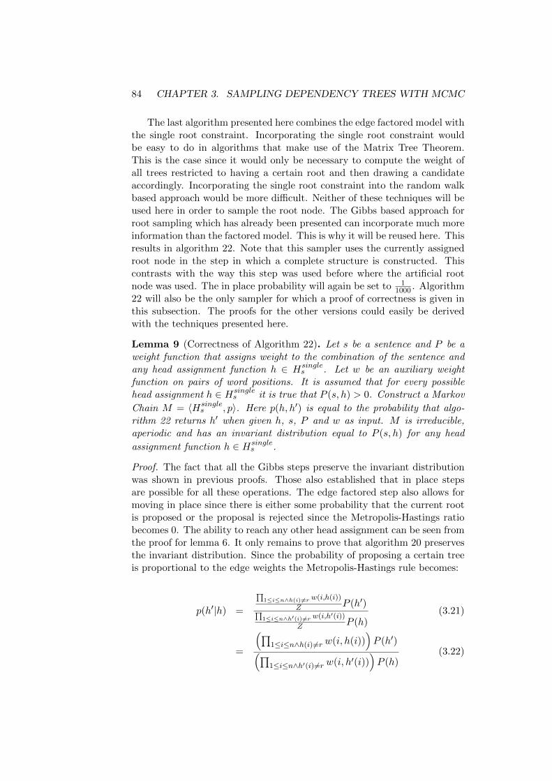
84 CHAPTER 3. SAMPLING DEPENDENCY TREES WITH MCMC
The last algorithm presented here combines the edge factored model withthe single root constraint. Incorporating the single root constraint wouldbe easy to do in algorithms that make use of the Matrix Tree Theorem.This is the case since it would only be necessary to compute the weight ofall trees restricted to having a certain root and then drawing a candidateaccordingly. Incorporating the single root constraint into the random walkbased approach would be more difficult. Neither of these techniques will beused here in order to sample the root node. The Gibbs based approach forroot sampling which has already been presented can incorporate much moreinformation than the factored model. This is why it will be reused here. Thisresults in algorithm 22. Note that this sampler uses the currently assignedroot node in the step in which a complete structure is constructed. Thiscontrasts with the way this step was used before where the artificial rootnode was used. The in place probability will again be set to 1
1000 . Algorithm22 will also be the only sampler for which a proof of correctness is given inthis subsection. The proofs for the other versions could easily be derivedwith the techniques presented here.
Lemma 9 (Correctness of Algorithm 22). Let s be a sentence and P be aweight function that assigns weight to the combination of the sentence andany head assignment function h ∈ Hsingle
s . Let w be an auxiliary weightfunction on pairs of word positions. It is assumed that for every possiblehead assignment h ∈ Hsingle
s it is true that P (s, h) > 0. Construct a Markov
Chain M = 〈Hsingles , p〉. Here p(h, h′) is equal to the probability that algo-
rithm 22 returns h′ when given h, s, P and w as input. M is irreducible,aperiodic and has an invariant distribution equal to P (s, h) for any head
assignment function h ∈ Hsingles .
Proof. The fact that all the Gibbs steps preserve the invariant distributionwas shown in previous proofs. Those also established that in place stepsare possible for all these operations. The edge factored step also allows formoving in place since there is either some probability that the current rootis proposed or the proposal is rejected since the Metropolis-Hastings ratiobecomes 0. The ability to reach any other head assignment can be seen fromthe proof for lemma 6. It only remains to prove that algorithm 20 preservesthe invariant distribution. Since the probability of proposing a certain treeis proportional to the edge weights the Metropolis-Hastings rule becomes:
p(h′|h) =
∏1≤i≤n∧h(i)6=r w(i,h(i))
Z P (h′)∏1≤i≤n∧h′(i)6=r w(i,h′(i))
Z P (h)(3.21)
=
(∏1≤i≤n∧h(i) 6=r w(i, h(i))
)P (h′)(∏
1≤i≤n∧h′(i) 6=r w(i, h′(i)))P (h)
(3.22)

3.4. SAMPLING WITH GLOBAL CHANGES 85
Algorithm 22 GibbsEdgeSingleRootSampler(HeadAssignment h, Sentences = 〈w1, . . . , wn, r〉, WeightFunction P, InPlaceProbability ip, WeightAp-proximation w)
1: h← GibbsHeadSampler(h, s, P, n, ip)2: for i ∈ {k|1 ≤ k ≤ n} do3: if h(i) = r then4: h′ ← SampleRandomArborescence(〈w1, . . . , wn〉, w, i)5: h′(i)← r6: wold ←
∏1≤j≤n∧j 6=iw(j, h(j))
7: wnew ←∏
1≤j≤n∧j 6=iw(j, h′(j))
8: p← woldP (s,h′)wnewP (s,h)
9: d← uniform draw from (0, 1)10: if d ≤ p then11: h← h′
12: end if13: end if14: heads← FindPossibleHeadsSingleRoot(i, h, n, r)15: h′ ← h16: for head ∈ heads do17: h′(i)← head18: q(head) = P (s, h′)19: end for20: j choose at random proportional to q21: h(i)← j22: end for23: return h
86 CHAPTER 3. SAMPLING DEPENDENCY TREES WITH MCMC
which is the ratio used in the algorithm.
A final remark needs to be made with respect to the choice of the approx-imate weight function for algorithm 22 and the other techniques presentedhere. The algorithm assumes that the function is fixed for all sampling steps.In the sampling of all dependency structures in a corpus, this does not meanthat the function has to be the same throughout. Instead the function maydepend on all other entries in the corpus that are currently left unchangedby the sampler. It would even be possible to allow the weight function todepend on past samples if techniques from adaptive MCMC are used [64].
It would be difficult to incorporate the constraint to projective structureswith the samplers given in this section. As stated before this could be moreeasily done by exploiting Eisners algorithm [32]. Since this algorithm isalready a well known tool it will not be investigated further here. The nextsection will introduce a global sampler that can more easily deal with suchhard restrictions on the admissible trees.
3.4.2 Sampling by Greedy Construction
The last section used an exact solution to an approximate problem in orderto generate a new proposal for a dependency tree. This section uses anapproximate solution to an approximate problem. This could seem like astep back, but the approximate problem used can be substantially strongerwhich may be a great advantage. The approximate solution used in thissection is based on the idea of greedy optimization. In order to apply thisin a sampling context a random element is necessary. This means that thesimple greedy approach is extended so that moves are more likely towardsbetter solutions but they are not guaranteed to always chose the best option.
The clearest inspiration for the technique, at least as far as the process-ing of dependency structures is concerned, is the so called transition basedparsing of sentences which has received a lot of attention in the literature[82]. In this paradigm a tree for a sentence is built up left to right using allthe decisions made up to this point as additional information for the parsingalgorithm. This approach can lead to choices being made that would turnout to be sub-optimal in light of information given later in the sentence [75].This is a weakness that the algorithm presented here unfortunately shares.Another connection is the step-by-step generation of the samples in that isalso used in in Sequential Monte Carlo Methods (SMC) [77, 14]. SMC hasbeen used before in order to generate samples in unsupervised POS tagging[31]. There are two important differences to the technique presented here.The first is the fact that SMC makes use of a number of candidates that aremaintained while a sample is generated. Using a number of candidates is anextension that could be made to the greedy algorithms. At the same time
3.4. SAMPLING WITH GLOBAL CHANGES 87
this is a complication that would make the presentation more difficult andis therefore left for further research. The second difference is the fact thatSMC places some requirements on the structure of the distribution that issampled. One example of these requirements is a restriction to sequences ofobservations and weight functions that have a Markov Chain structure. Thisrequirement is no longer necessary for the Greedy sampler since it ensuresits correctness through a “surrounding” Metropolis-Hastings step.
The general idea of the sampler is as follows. Some approximation g ofthe actual weight function P is given. This approximation assigns weight toincomplete versions of the head assignment function. This is necessary sincea dependency tree is to be built step by step. In some models, especiallythose that compute the probability of a dependency tree edge by edge, itwill be possible to use the actual weight function and just ignore the wordsthat have not yet been assigned any heads. The algorithm then sweepsover the words in the sentence in some order and constructs a new headassignments function h′. The assignment for the next word in the sweep issampled proportionally to the weight of the head assignments if a certainsetting is added.
The order of the sweep is randomized. The reasoning for this is the factthat previous choices restrict the choices that can still be made. Considerfor example choosing the root node in cases where the single root constraintis used. Once a word has been attached to the artificial root node no otherwords can be attached there. For this reason it would be interesting to letevery word “have a chance” at selecting its head first. There has been someinvestigation into the effects of schedules in with which a greedy sweep isimplemented [27] but this is not be investigated further here.
The reason that such a sampler has not been proposed so far seemstwofold. The first is a strong focus on Gibbs like methods. The use of themore general Metropolis-Hastings techniques has received less attention, butthey are the key to making the greedy construction work. The other reasonis the fact that so far global approaches have been focused on charts in orderto correctly compute the proposal probabilities. In this work the problemcan be circumvented because once the order in which heads are assigned isfixed, it is possible to compute the probability for any dependency tree tobe proposed.
Two further concerns need to be addressed in developing the greedysampler. They both concern the invariant distribution that is used. Thefirst is the fact that multiple ways of sweeping over the word positions implymore complicated proposal distributions which has the potential to make theapplication of the Metropolis-Hastings rule much more difficult. In orderto address this problem a version of the Metropolis-Hastings rule will beintroduced that allows for a way around this problem.
Definition 13 (Piece-by-Piece Metropolis-Hastings Rule). Assume there
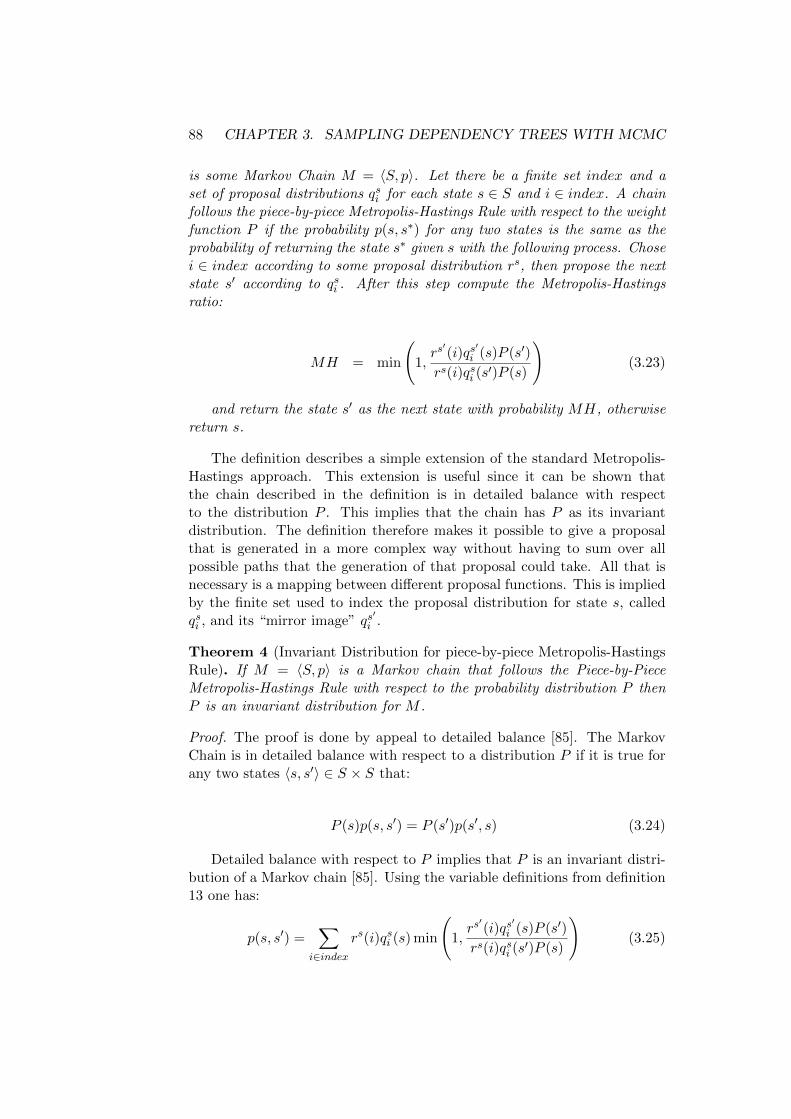
88 CHAPTER 3. SAMPLING DEPENDENCY TREES WITH MCMC
is some Markov Chain M = 〈S, p〉. Let there be a finite set index and aset of proposal distributions qsi for each state s ∈ S and i ∈ index. A chainfollows the piece-by-piece Metropolis-Hastings Rule with respect to the weightfunction P if the probability p(s, s∗) for any two states is the same as theprobability of returning the state s∗ given s with the following process. Chosei ∈ index according to some proposal distribution rs, then propose the nextstate s′ according to qsi . After this step compute the Metropolis-Hastingsratio:
MH = min
(1,rs′(i)qs
′i (s)P (s′)
rs(i)qsi (s′)P (s)
)(3.23)
and return the state s′ as the next state with probability MH, otherwisereturn s.
The definition describes a simple extension of the standard Metropolis-Hastings approach. This extension is useful since it can be shown thatthe chain described in the definition is in detailed balance with respectto the distribution P . This implies that the chain has P as its invariantdistribution. The definition therefore makes it possible to give a proposalthat is generated in a more complex way without having to sum over allpossible paths that the generation of that proposal could take. All that isnecessary is a mapping between different proposal functions. This is impliedby the finite set used to index the proposal distribution for state s, calledqsi , and its “mirror image” qs
′i .
Theorem 4 (Invariant Distribution for piece-by-piece Metropolis-HastingsRule). If M = 〈S, p〉 is a Markov chain that follows the Piece-by-PieceMetropolis-Hastings Rule with respect to the probability distribution P thenP is an invariant distribution for M .
Proof. The proof is done by appeal to detailed balance [85]. The MarkovChain is in detailed balance with respect to a distribution P if it is true forany two states 〈s, s′〉 ∈ S × S that:
P (s)p(s, s′) = P (s′)p(s′, s) (3.24)
Detailed balance with respect to P implies that P is an invariant distri-bution of a Markov chain [85]. Using the variable definitions from definition13 one has:
p(s, s′) =∑
i∈indexrs(i)qsi (s) min
(1,rs′(i)qs
′i (s)P (s′)
rs(i)qsi (s′)P (s)
)(3.25)
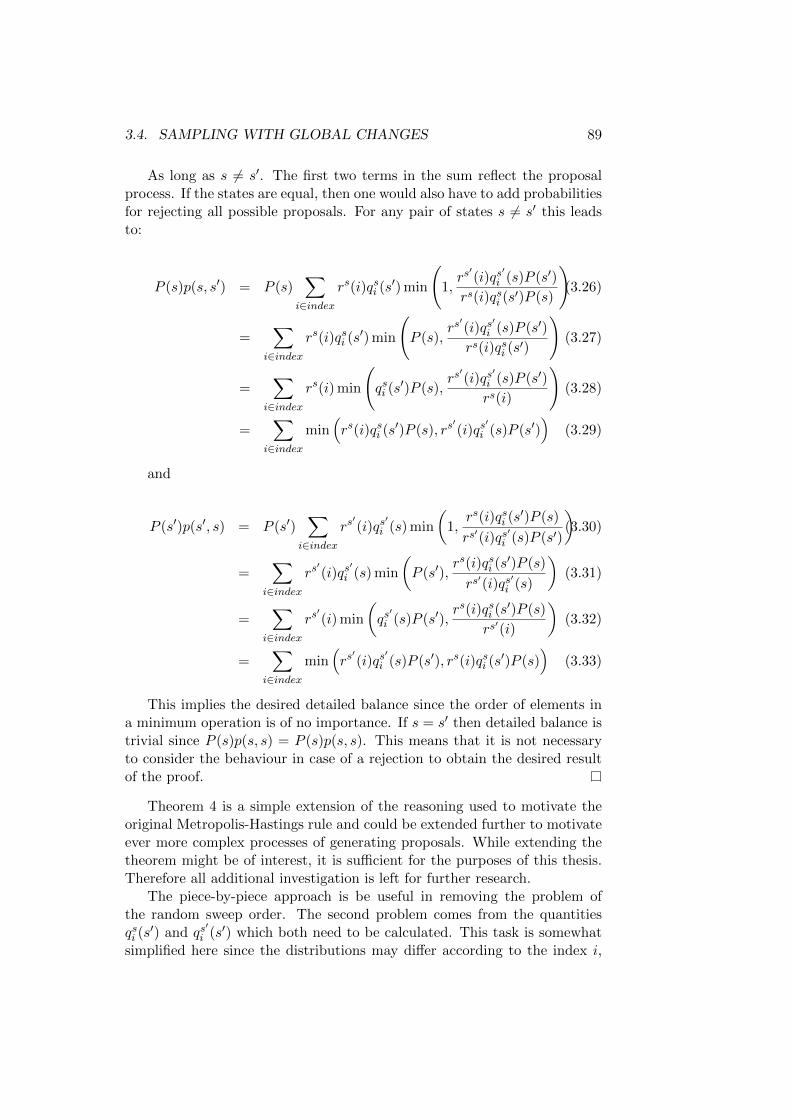
3.4. SAMPLING WITH GLOBAL CHANGES 89
As long as s 6= s′. The first two terms in the sum reflect the proposalprocess. If the states are equal, then one would also have to add probabilitiesfor rejecting all possible proposals. For any pair of states s 6= s′ this leadsto:
P (s)p(s, s′) = P (s)∑
i∈indexrs(i)qsi (s′) min
(1,rs′(i)qs
′i (s)P (s′)
rs(i)qsi (s′)P (s)
)(3.26)
=∑
i∈indexrs(i)qsi (s′) min
(P (s),
rs′(i)qs
′i (s)P (s′)
rs(i)qsi (s′)
)(3.27)
=∑
i∈indexrs(i) min
(qsi (s′)P (s),
rs′(i)qs
′i (s)P (s′)
rs(i)
)(3.28)
=∑
i∈indexmin
(rs(i)qsi (s′)P (s), rs
′(i)qs
′i (s)P (s′)
)(3.29)
and
P (s′)p(s′, s) = P (s′)∑
i∈indexrs′(i)qs
′i (s) min
(1,rs(i)qsi (s′)P (s)
rs′(i)qs′
i (s)P (s′)
)(3.30)
=∑
i∈indexrs′(i)qs
′i (s) min
(P (s′),
rs(i)qsi (s′)P (s)
rs′(i)qs′
i (s)
)(3.31)
=∑
i∈indexrs′(i) min
(qs′
i (s)P (s′),rs(i)qsi (s′)P (s)
rs′(i)
)(3.32)
=∑
i∈indexmin
(rs′(i)qs
′i (s)P (s′), rs(i)qsi (s′)P (s)
)(3.33)
This implies the desired detailed balance since the order of elements ina minimum operation is of no importance. If s = s′ then detailed balance istrivial since P (s)p(s, s) = P (s)p(s, s). This means that it is not necessaryto consider the behaviour in case of a rejection to obtain the desired resultof the proof.
Theorem 4 is a simple extension of the reasoning used to motivate theoriginal Metropolis-Hastings rule and could be extended further to motivateever more complex processes of generating proposals. While extending thetheorem might be of interest, it is sufficient for the purposes of this thesis.Therefore all additional investigation is left for further research.
The piece-by-piece approach is be useful in removing the problem ofthe random sweep order. The second problem comes from the quantitiesqsi (s′) and qs
′i (s′) which both need to be calculated. This task is somewhat
simplified here since the distributions may differ according to the index i,
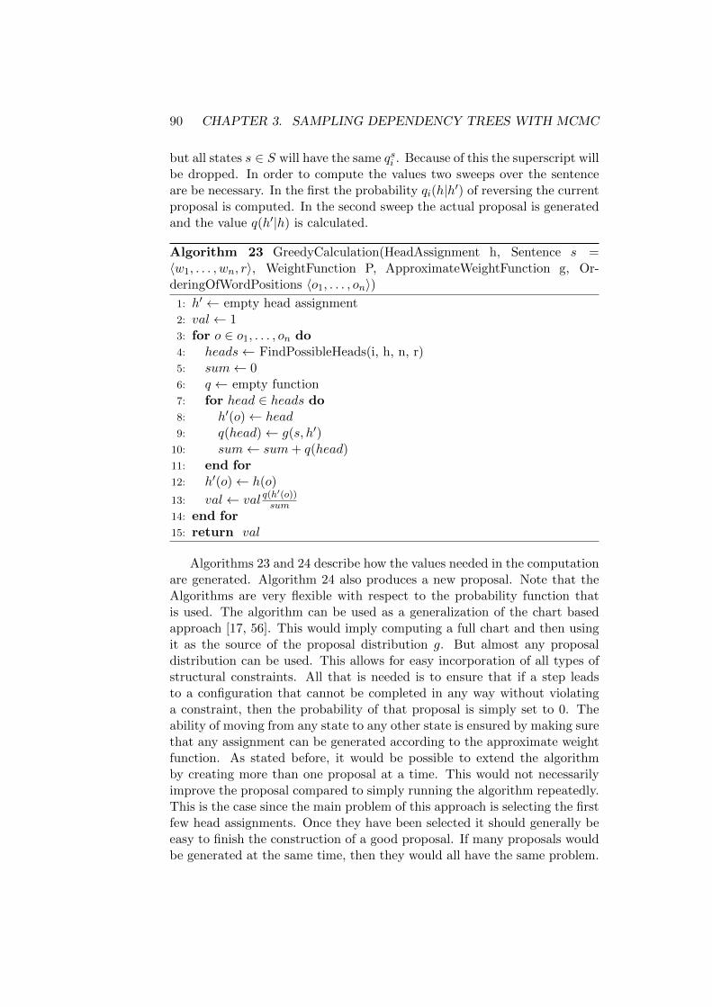
90 CHAPTER 3. SAMPLING DEPENDENCY TREES WITH MCMC
but all states s ∈ S will have the same qsi . Because of this the superscript willbe dropped. In order to compute the values two sweeps over the sentenceare be necessary. In the first the probability qi(h|h′) of reversing the currentproposal is computed. In the second sweep the actual proposal is generatedand the value q(h′|h) is calculated.
Algorithm 23 GreedyCalculation(HeadAssignment h, Sentence s =〈w1, . . . , wn, r〉, WeightFunction P, ApproximateWeightFunction g, Or-deringOfWordPositions 〈o1, . . . , on〉)
1: h′ ← empty head assignment2: val← 13: for o ∈ o1, . . . , on do4: heads← FindPossibleHeads(i, h, n, r)5: sum← 06: q ← empty function7: for head ∈ heads do8: h′(o)← head9: q(head)← g(s, h′)
10: sum← sum+ q(head)11: end for12: h′(o)← h(o)
13: val← val q(h′(o))sum
14: end for15: return val
Algorithms 23 and 24 describe how the values needed in the computationare generated. Algorithm 24 also produces a new proposal. Note that theAlgorithms are very flexible with respect to the probability function thatis used. The algorithm can be used as a generalization of the chart basedapproach [17, 56]. This would imply computing a full chart and then usingit as the source of the proposal distribution g. But almost any proposaldistribution can be used. This allows for easy incorporation of all types ofstructural constraints. All that is needed is to ensure that if a step leadsto a configuration that cannot be completed in any way without violatinga constraint, then the probability of that proposal is simply set to 0. Theability of moving from any state to any other state is ensured by making surethat any assignment can be generated according to the approximate weightfunction. As stated before, it would be possible to extend the algorithmby creating more than one proposal at a time. This would not necessarilyimprove the proposal compared to simply running the algorithm repeatedly.This is the case since the main problem of this approach is selecting the firstfew head assignments. Once they have been selected it should generally beeasy to finish the construction of a good proposal. If many proposals wouldbe generated at the same time, then they would all have the same problem.
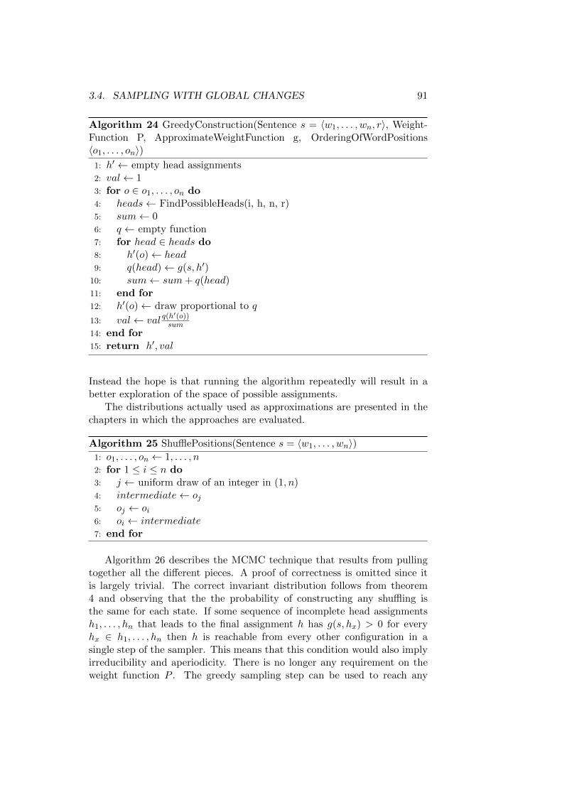
3.4. SAMPLING WITH GLOBAL CHANGES 91
Algorithm 24 GreedyConstruction(Sentence s = 〈w1, . . . , wn, r〉, Weight-Function P, ApproximateWeightFunction g, OrderingOfWordPositions〈o1, . . . , on〉)
1: h′ ← empty head assignments2: val← 13: for o ∈ o1, . . . , on do4: heads← FindPossibleHeads(i, h, n, r)5: sum← 06: q ← empty function7: for head ∈ heads do8: h′(o)← head9: q(head)← g(s, h′)
10: sum← sum+ q(head)11: end for12: h′(o)← draw proportional to q
13: val← val q(h′(o))sum
14: end for15: return h′, val
Instead the hope is that running the algorithm repeatedly will result in abetter exploration of the space of possible assignments.
The distributions actually used as approximations are presented in thechapters in which the approaches are evaluated.
Algorithm 25 ShufflePositions(Sentence s = 〈w1, . . . , wn〉)1: o1, . . . , on ← 1, . . . , n2: for 1 ≤ i ≤ n do3: j ← uniform draw of an integer in (1, n)4: intermediate← oj5: oj ← oi6: oi ← intermediate7: end for
Algorithm 26 describes the MCMC technique that results from pullingtogether all the different pieces. A proof of correctness is omitted since itis largely trivial. The correct invariant distribution follows from theorem4 and observing that the the probability of constructing any shuffling isthe same for each state. If some sequence of incomplete head assignmentsh1, . . . , hn that leads to the final assignment h has g(s, hx) > 0 for everyhx ∈ h1, . . . , hn then h is reachable from every other configuration in asingle step of the sampler. This means that this condition would also implyirreducibility and aperiodicity. There is no longer any requirement on theweight function P . The greedy sampling step can be used to reach any
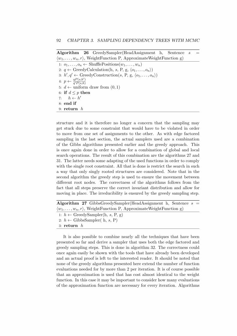
92 CHAPTER 3. SAMPLING DEPENDENCY TREES WITH MCMC
Algorithm 26 GreedySampler(HeadAssignment h, Sentence s =〈w1, . . . , wn, r〉, WeightFunction P, ApproximateWeightFunction g)
1: o1, . . . , on ← ShufflePositions(w1, . . . , wn)2: q ← GreedyCalculation(h, s, P, g, 〈o1, . . . , on〉)3: h′, q′ ← GreedyConstruction(s, P, g, 〈o1, . . . , on〉)4: p← qP (s,h′)
q′P (s,h)
5: d← uniform draw from (0, 1)6: if d ≤ p then7: h← h′
8: end if9: return h
structure and it is therefore no longer a concern that the sampling mayget stuck due to some constraint that would have to be violated in orderto move from one set of assignments to the other. As with edge factoredsampling in the last section, the actual samplers used are a combinationof the Gibbs algorithms presented earlier and the greedy approach. Thisis once again done in order to allow for a combination of global and localsearch operations. The result of this combination are the algorithms 27 and31. The latter needs some adapting of the used functions in order to complywith the single root constraint. All that is done is restrict the search in sucha way that only singly rooted structures are considered. Note that in thesecond algorithm the greedy step is used to ensure the movement betweendifferent root nodes. The correctness of the algorithms follows from thefact that all steps preserve the correct invariant distribution and allow formoving in place. The irreducibility is ensured by the greedy sampling step.
Algorithm 27 GibbsGreedySampler(HeadAssignment h, Sentence s =〈w1, . . . , wn, r〉, WeightFunction P, ApproximateWeightFunction g)
1: h← GreedySampler(h, s, P, g)2: h← GibbsSampler( h, s, P)3: return h
It is also possible to combine nearly all the techniques that have beenpresented so far and derive a sampler that uses both the edge factored andgreedy sampling steps. This is done in algorithm 32. The correctness couldonce again easily be shown with the tools that have already been developedand an actual proof is left to the interested reader. It should be noted thatnone of the greedy algorithms presented here extend the number of functionevaluations needed for by more than 2 per iteration. It is of course possiblethat an approximation is used that has cost almost identical to the weightfunction. In this case it may be important to consider how many evaluationsof the approximation function are necessary for every iteration. Algorithms

3.4. SAMPLING WITH GLOBAL CHANGES 93
Algorithm 28 GreedySingleRootCalculation(HeadAssignment h, Sentences = 〈w1, . . . , wn, r〉, WeightFunction P, ApproximateWeightFunction g, Or-deringOfWordPositions 〈o1, . . . , on〉)
1: h′ ← empty head assignments2: val← 13: for o ∈ o1, . . . , on do4: heads← FindPossibleHeadsSingleRoot(i, h, n, r)5: sum← 06: q ← empty function7: for head ∈ heads do8: h′(o)← head9: q(head)← g(s, h′)
10: sum← sum+ q(head)11: end for12: h′(o)← h(o)
13: val← val q(h′(o))sum
14: end for15: return val
Algorithm 29 GreedySingleRootConstruction(Sentence s =〈w1, . . . , wn, r〉, WeightFunction P ApproximateWeightFunction g, Or-deringOfWordPositions 〈o1, . . . , on〉)
1: h′ ← empty head assignments2: val← 13: for o ∈ o1, . . . , on do4: heads← FindPossibleHeadsSingleRoot(i, h, n, r)5: sum← 06: q ← empty function7: for head ∈ heads do8: h′(o)← head9: q(head)← g(s, h′)
10: sum← sum+ q(head)11: end for12: h′(o)← draw proportional to q
13: val← val q(h′(o))sum
14: end for15: return h′, val

94 CHAPTER 3. SAMPLING DEPENDENCY TREES WITH MCMC
Algorithm 30 GreedySingleRootSampler(HeadAssignment h, Sentence s =〈w1, . . . , wn, r〉, WeightFunction P, ApproximateWeightFunction g)
1: o1, . . . , on ← ShufflePositions(w1, . . . , wn)2: q ← GreedySingleRootCalculation(h, s, P, g, 〈o1, . . . , on〉)3: h′, q′ ← GreedySingleRootConstruction(s, P, g, 〈o1, . . . , on〉)4: p← qP (s,h′)
q′P (s,h)
5: d← uniform draw from (0, 1)6: if d ≤ p then7: h← h′
8: end if9: return h
Algorithm 31 GibbsGreedySingleRootSampler(HeadAssignment h, Sen-tence s = 〈w1, . . . , wn, r〉, WeightFunction P, ApproximateWeightFunctiong)
1: h← GreedySingleRootSampler(h, s, P, g)2: for i ∈ {k|1 ≤ k ≤ n} do3: if h(i) = r then4: continue with next iteration step5: end if6: heads← FindPossibleHeadsSingleRoot(i, h, n, r)7: h′ ← h8: for head ∈ heads do9: h′(i)← head
10: q(head) = P (s, h′)11: end for12: j choose at random proportional to q13: h(i)← j14: end for15: return h
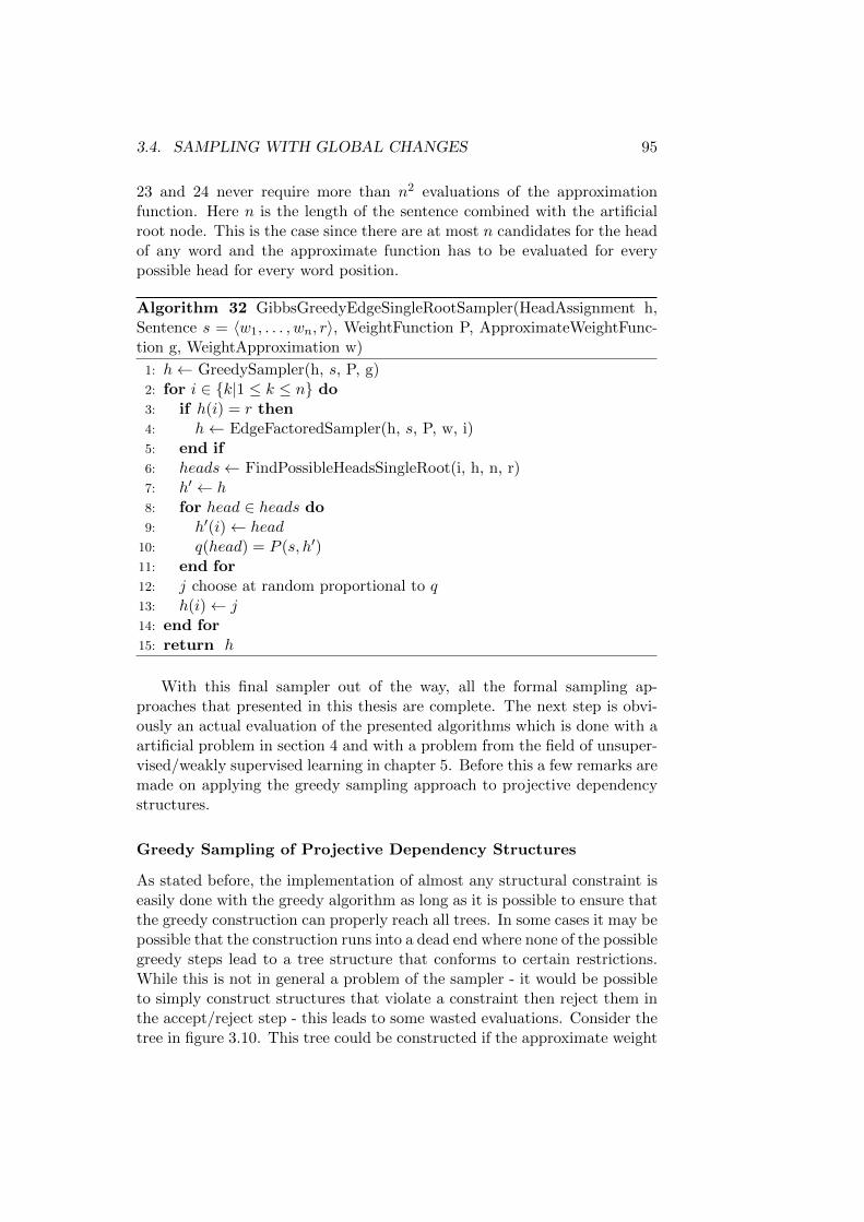
3.4. SAMPLING WITH GLOBAL CHANGES 95
23 and 24 never require more than n2 evaluations of the approximationfunction. Here n is the length of the sentence combined with the artificialroot node. This is the case since there are at most n candidates for the headof any word and the approximate function has to be evaluated for everypossible head for every word position.
Algorithm 32 GibbsGreedyEdgeSingleRootSampler(HeadAssignment h,Sentence s = 〈w1, . . . , wn, r〉, WeightFunction P, ApproximateWeightFunc-tion g, WeightApproximation w)
1: h← GreedySampler(h, s, P, g)2: for i ∈ {k|1 ≤ k ≤ n} do3: if h(i) = r then4: h← EdgeFactoredSampler(h, s, P, w, i)5: end if6: heads← FindPossibleHeadsSingleRoot(i, h, n, r)7: h′ ← h8: for head ∈ heads do9: h′(i)← head
10: q(head) = P (s, h′)11: end for12: j choose at random proportional to q13: h(i)← j14: end for15: return h
With this final sampler out of the way, all the formal sampling ap-proaches that presented in this thesis are complete. The next step is obvi-ously an actual evaluation of the presented algorithms which is done with aartificial problem in section 4 and with a problem from the field of unsuper-vised/weakly supervised learning in chapter 5. Before this a few remarks aremade on applying the greedy sampling approach to projective dependencystructures.
Greedy Sampling of Projective Dependency Structures
As stated before, the implementation of almost any structural constraint iseasily done with the greedy algorithm as long as it is possible to ensure thatthe greedy construction can properly reach all trees. In some cases it may bepossible that the construction runs into a dead end where none of the possiblegreedy steps lead to a tree structure that conforms to certain restrictions.While this is not in general a problem of the sampler - it would be possibleto simply construct structures that violate a constraint then reject them inthe accept/reject step - this leads to some wasted evaluations. Consider thetree in figure 3.10. This tree could be constructed if the approximate weight
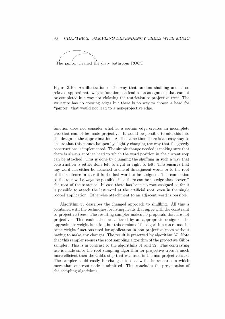
96 CHAPTER 3. SAMPLING DEPENDENCY TREES WITH MCMC
The janitor cleaned the dirty bathroom ROOT
Figure 3.10: An illustration of the way that random shuffling and a toorelaxed approximate weight function can lead to an assignment that cannotbe completed in a way not violating the restriction to projective trees. Thestructure has no crossing edges but there is no way to choose a head for“janitor” that would not lead to a non-projective edge.
function does not consider whether a certain edge creates an incompletetree that cannot be made projective. It would be possible to add this intothe design of the approximation. At the same time there is an easy way toensure that this cannot happen by slightly changing the way that the greedyconstructions is implemented. The simple change needed is making sure thatthere is always another head to which the word position in the current stepcan be attached. This is done by changing the shuffling in such a way thatconstruction is either done left to right or right to left. This ensures thatany word can either be attached to one of its adjacent words or to the rootof the sentence in case it is the last word to be assigned. The connectionto the root will always be possible since there can be no edge that “covers”the root of the sentence. In case there has been no root assigned so far itis possible to attach the last word at the artificial root, even in the singlerooted application. Otherwise attachment to an adjacent word is possible.
Algorithm 33 describes the changed approach to shuffling. All this iscombined with the techniques for listing heads that agree with the constraintto projective trees. The resulting sampler makes no proposals that are notprojective. This could also be achieved by an appropriate design of theapproximate weight function, but this version of the algorithm can re-use thesame weight functions used for application in non-projective cases withouthaving to make any changes. The result is presented by algorithm 37. Notethat this sampler re-uses the root sampling algorithm of the projective Gibbssampler. This is in contrast to the algorithms 31 and 32. This contrastinguse is made since the root sampling algorithm for projective trees is muchmore efficient then the Gibbs step that was used in the non-projective case.The sampler could easily be changed to deal with the scenario in whichmore than one root node is admitted. This concludes the presentation ofthe sampling algorithms.

3.4. SAMPLING WITH GLOBAL CHANGES 97
Algorithm 33 ShufflePositionsProjective(Sentence s = 〈w1, . . . , wn〉)1: if uniform draw from (0, 1) is less than 0.5 then2: return 1, . . . , n3: else4: return n, . . . , 15: end if
Algorithm 34 GreedyProjectiveSingleRootCalculation(HeadAssignmenth, Sentence s = 〈w1, . . . , wn, r〉, WeightFunction P, ApproximateWeight-Function g, OrderingOfWordPositions 〈o1, . . . , on〉)
1: h′ ← empty head assignments2: val← 13: for o ∈ o1, . . . , on do4: heads← FindPossibleHeadsSingleRootProjective(i, h, n, r)5: sum← 06: q ← empty function7: for head ∈ heads do8: h′(o)← head9: q(head)← g(s, h′)
10: sum← sum+ q(head)11: end for12: h′(o)← h(o)
13: val← val q(h′(o))sum
14: end for15: return val
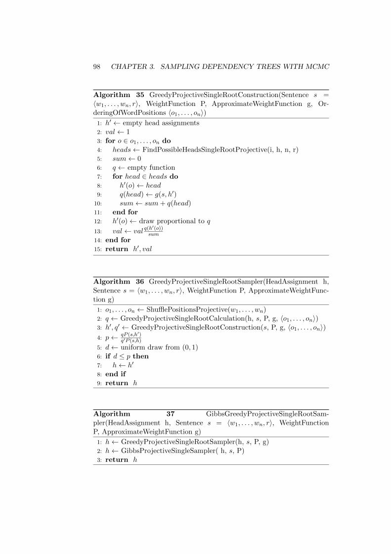
98 CHAPTER 3. SAMPLING DEPENDENCY TREES WITH MCMC
Algorithm 35 GreedyProjectiveSingleRootConstruction(Sentence s =〈w1, . . . , wn, r〉, WeightFunction P, ApproximateWeightFunction g, Or-deringOfWordPositions 〈o1, . . . , on〉)
1: h′ ← empty head assignments2: val← 13: for o ∈ o1, . . . , on do4: heads← FindPossibleHeadsSingleRootProjective(i, h, n, r)5: sum← 06: q ← empty function7: for head ∈ heads do8: h′(o)← head9: q(head)← g(s, h′)
10: sum← sum+ q(head)11: end for12: h′(o)← draw proportional to q
13: val← val q(h′(o))sum
14: end for15: return h′, val
Algorithm 36 GreedyProjectiveSingleRootSampler(HeadAssignment h,Sentence s = 〈w1, . . . , wn, r〉, WeightFunction P, ApproximateWeightFunc-tion g)
1: o1, . . . , on ← ShufflePositionsProjective(w1, . . . , wn)2: q ← GreedyProjectiveSingleRootCalculation(h, s, P, g, 〈o1, . . . , on〉)3: h′, q′ ← GreedyProjectiveSingleRootConstruction(s, P, g, 〈o1, . . . , on〉)4: p← qP (s,h′)
q′P (s,h)
5: d← uniform draw from (0, 1)6: if d ≤ p then7: h← h′
8: end if9: return h
Algorithm 37 GibbsGreedyProjectiveSingleRootSam-pler(HeadAssignment h, Sentence s = 〈w1, . . . , wn, r〉, WeightFunctionP, ApproximateWeightFunction g)
1: h← GreedyProjectiveSingleRootSampler(h, s, P, g)2: h← GibbsProjectiveSingleSampler( h, s, P)3: return h
3.5. CONCLUSION 99
3.5 Conclusion
This chapter achieved two primary goals: it took a number of simple, headby head sampling techniques based on approaches introduced previously inthe literature and showed that they are applicable to a number of differentMCMC settings that include some hard restrictions on the way dependencytrees can be constructed. It was also shown that these algorithms defineprovably correct MCMC schemes.
Besides the basic approaches the chapter also gave some global ap-proaches that extend previous research in this direction. The greedy samplercan be used with complex proposal distributions and is a generalization ofmost techniques proposed before. The edge factored MCMC scheme is basedon a very strong restriction of the proposal distribution but allows for an ex-act proposal from this distribution. Both approaches are intended to lessenthe impact of local optima.
The following chapters are intended to evaluate the presented algorithmsand show their strengths and weaknesses. The algorithms came in a numberof versions and due to limitations of space it is necessary to focus on a few ofthem. Since a major theme of this thesis is the use of structural constraints,only single rooted versions of the different algorithms are evaluated. At thesame time both the projective and non-projective versions are used. This isthe case since some techniques only apply to one of these possible settings.The fact that it is easy to combine samplers is a strength of MCMC andthe extended versions of the global samplers are used throughout. This waythe local approaches can find the optima that the global steps will make itpossible to escape.

100 CHAPTER 3. SAMPLING DEPENDENCY TREES WITH MCMC
Chapter 4
Convergence Evaluation onan Artificial Problem
4.1 Introduction
In this chapter the sampling techniques presented in chapter 3.3 are eval-uated on a sampling problem with an artificial distribution. The task isartificial in so far as it does not immediately come from any Natural Lan-guage Processing task and it allows for the analytic computation of somestatistic of interest. Assume that a sample is drawn from such an test dis-tribution by using Markov Chain Monte Carlo methods, it is then possibleto compute the statistic from the draw. The difference between the valuecalculated from the MCMC run and the correct value for the evaluationdistribution can then be compared. This possibility contrasts sharply withmost actual use cases for MCMC. There the actual value would often haveto be computed by brute force or by some approximation algorithm thatcan be used as an alternative to MCMC. One such example will be theunsupervised learning of dependency structures that is used for evaluationin chapter 5. In that chapter the main statistic investigated is the highestprobability assignment that has been found after a certain number of steps.While this statistic is interesting for determining how quickly the processmoves towards maxima of the probability function and how strong the foundmaxima are, the results are not completely instructive for investigating thebehaviour of a sampling algorithm. If the task is purely the maximization ofsome function value, then there are techniques for global optimization thatcould very well have a much better performance [97, 116]. Expectationsover all possible assignments, the main goal of MCMC approaches, are com-pletely impossible to compute in any reasonable time. This means that theevaluation results generated with an artificial distribution are a necessarypart of any complete evaluation of MCMC sampling algorithms.
Another alternative to artificial problems would be running different
101
102 CHAPTER 4. ARTIFICIAL EVALUATION
algorithms and comparing their results. This technique is often used toestablish the number of iterations that are needed until the results from aMCMC scheme become reliable [40]. In this case multiple Markov Chainsimulations are run at the same time and some statistic is calculated thatexpresses how close their results are. The assumption is usually made thatonce the sample statistics of all chains tend towards the same result theyhave converged. This approach has limited usefulness for the evaluation ofdifferent algorithms. When the chains converge towards different values,then it becomes unclear which is the correct one. It could also be the casethat all the algorithms tend towards the same, incorrect value.
With some motivation for the evaluation technique out of the way itbecomes necessary to explain what would constitute “good” behaviour ofa MCMC sampler in the experimental evaluation. Instead of running theprocess until some predefined statistic is reached to some level of accuracy,the experiments presented here were run for a fixed number of steps and thebehaviour was tracked throughout the complete run. This is more likely toresemble a “real” application situation. Users of an MCMC algorithm willoften only have a limited computational budget. Within this budget thesampling algorithms will usually be run. Whatever result has been reachedhas to be used. If the sampling algorithm reaches convergence within the al-lotted time, then it is also possible to make a statement about the number ofiterations necessary to reach this convergence. As will be seen in the evalua-tion results, the algorithms do not always converge to within any reasonableaccuracy. The value of some summary statistic of a single chain or a numberof chains being used to simulated the target distribution is presented. Fora good MCMC algorithm the summary statistic will quickly move towardsthe value derived by analysis. It is also tracked how many computationalresources have been used up to a certain iteration step. The computationalresources are measured in terms of the evaluations that have been made ofthe probability function and the evaluations that have been made of theauxiliary functions needed for the greedy sampling algorithms and the edgefactored techniques. This evaluation of the resource requirements is choseninstead of measuring things like working memory usage or the number ofprocessor steps taken. The reason that things like the memory or processingsteps are ignored is that fact that these statistics are dependent on the exactimplementation of the algorithms. As stated during the presentation of thealgorithms, it is assumed that the runtime of any sampler will be dominatedby the time spend evaluating the mentioned functions. The result of thisdiscussion are the following criteria for a good sampler:
• It correctly predicts the statistic of interest within the allotted numberof samples drawn up to some tolerance.
• It makes use of a small number of function evaluations.
4.1. INTRODUCTION 103
It should be noted that the MCMC algorithms evaluated are the tech-niques used for single rooted sampling both projective and non-projective.This means that algorithms involving all the tools developed are consid-ered. The focus on single rooted algorithms is chosen here since dealingwith structural restrictions is one of the main topics of this thesis and thisis an instance of such a restriction that can be combined with all the othertechniques.
This chapter proceeds as follows. First it is established what kind ofprobability function is used for the evaluation. Following this it is necessaryto define the auxiliary functions used in sampling. Afterwards the types ofstatistics kept will be explained. The choice of target function is obviouslyrelated to the values tracked, since the function determines what kind ofstatistics can be predicted analytically. Finally the chapter can concludewith the discussion of the evaluation results for different settings of theartificial task.
4.1.1 A Note on the Development of the Algorithms
In the presentation of the evaluation results it turns out that some samplershave severe problems with the evaluation task presented here. The problemsthey exhibited is generally not with finding at least one optimum of thetarget function but instead with dealing correctly with multiple optima.From the results one could get the impression that the sampling algorithmsmay have been implemented incorrectly. It is of course never possible toexclude a programming error. But all implementations have been testedwith the target function and they do in fact converge reliably given a fewthousand iteration steps and averaging of five parallel chains. These resultsare not presented here since the same statement could be made for all thealgorithms. It is also true that running any sampler for that many steps onmore than a few short sentence would be completely infeasible in almost allsettings. Therefore the decision was made to present the results includingthe failures of some of the algorithms on some runs. These results areassumed to be more helpful to the reader in picking tools for a particularproblem that he or she wants to solve. The implementation of the MCMCalgorithms and the benchmarking tools will also be made publicly availableopen source code. This will allow the interested reader to reproduce thebenchmarking results and check the algorithms.
The function used for evaluation in this section is not the only one againstwhich the samplers where checked for correctness. In fact there is an impor-tant lesson learned from the development process: Sampling from the uni-form distribution, i.e. the probability function that assigns equals weightto every dependency tree, is extremely useful in testing and developing acorrect dependency sampler. While the problem of correctly predicting thatevery tree should occur equally often does not reveal much about the per-
104 CHAPTER 4. ARTIFICIAL EVALUATION
formance of the algorithm, since most moves will be readily accepted, itdoes point out even small errors in the calculation of transition probabili-ties. When these probabilities are calculated it is often the case that only asmall fraction of their weight is determined by the elements necessary for thecorrectness of the sampling algorithm such as the Metropolis-Hastings rule.The majority of the weight will be determined by the function that is eval-uated and an algorithm might seem to perform correctly even when it hassome small programming error. For this reason the uniform distribution is avery good guide in the programming and testing of actual implementationsof dependency sampling algorithms. The weights of the different trees areall equal and will generally contribute a net zero effect to the sampling pro-cess. A small error in the algorithm will then lead to a completely incorrectresult in the MCMC approximation to the uniform distribution and this willreveal any possible errors. Since the uniform distribution for dependencystructures can only be correctly sampled by visiting every possible head as-signment at the same rate, the uniform probability function will also revealif a chain is not actually irreducible since possible assignment functions thatshould be visited fairly early in the sampling process will never be reached.
All algorithms presented here produced correct samples from the uni-form distribution. As stated before, the results that are derived from theuniform sampling scenario are not very interesting for a performance evalua-tion. It is a useful takeaway from the development process that the uniformdistribution can be instrumental in uncovering programming errors.
4.2 The Probability Function
In this section the probability function for the artificial evaluation is intro-duced. The function is based on two ideas. Models for dependency parsingare often used to select a single correct head assignment which is then usedin further processing tasks [42, 16, 83, 75] and there is a general tendency independency structures to prefer a small subset of the possible dependencyassignments compared to the full set of possibilities [110, 111]. For thisreason it can generally be assumed that a “good” model for dependencyparsing will assign a great amount of weight to a few dependency struc-tures. This is modelled by the evaluation problem giving most of its weightto a few dependency trees. The second inspiration is the problem of dealingwith multiple unconnected areas in which the probability function takes ahigh value, i.e. dealing with local optima. This is an important problem inthe design of MCMC algorithms [64]. Most algorithms have little problemwith moving towards an optimum and then moving closely around it. It ismuch harder to have the algorithms traverse correctly through valleys in theweight function. Because of this the probability function is designed in sucha way that there are two obvious and distinct optima.
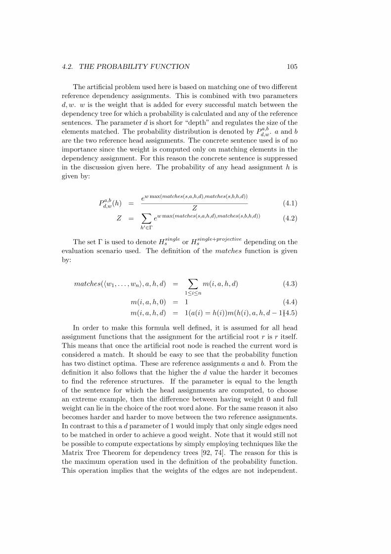
4.2. THE PROBABILITY FUNCTION 105
The artificial problem used here is based on matching one of two differentreference dependency assignments. This is combined with two parametersd,w. w is the weight that is added for every successful match between thedependency tree for which a probability is calculated and any of the referencesentences. The parameter d is short for “depth” and regulates the size of theelements matched. The probability distribution is denoted by P a,b
d,w. a and bare the two reference head assignments. The concrete sentence used is of noimportance since the weight is computed only on matching elements in thedependency assignment. For this reason the concrete sentence is suppressedin the discussion given here. The probability of any head assignment h isgiven by:
P a,bd,w(h) =
ew max(matches(s,a,h,d),matches(s,b,h,d))
Z(4.1)
Z =∑h′∈Γ
ew max(matches(s,a,h,d),matches(s,b,h,d)) (4.2)
The set Γ is used to denote Hsingles or Hsingle+projective
s depending on theevaluation scenario used. The definition of the matches function is givenby:
matches(〈w1, . . . , wn〉, a, h, d) =∑
1≤i≤nm(i, a, h, d) (4.3)
m(i, a, h, 0) = 1 (4.4)
m(i, a, h, d) = 1(a(i) = h(i))m(h(i), a, h, d− 1)(4.5)
In order to make this formula well defined, it is assumed for all headassignment functions that the assignment for the artificial root r is r itself.This means that once the artificial root node is reached the current word isconsidered a match. It should be easy to see that the probability functionhas two distinct optima. These are reference assignments a and b. From thedefinition it also follows that the higher the d value the harder it becomesto find the reference structures. If the parameter is equal to the lengthof the sentence for which the head assignments are computed, to choosean extreme example, then the difference between having weight 0 and fullweight can lie in the choice of the root word alone. For the same reason it alsobecomes harder and harder to move between the two reference assignments.In contrast to this a d parameter of 1 would imply that only single edges needto be matched in order to achieve a good weight. Note that it would still notbe possible to compute expectations by simply employing techniques like theMatrix Tree Theorem for dependency trees [92, 74]. The reason for this isthe maximum operation used in the definition of the probability function.This operation implies that the weights of the edges are not independent.
106 CHAPTER 4. ARTIFICIAL EVALUATION
Assume that d = 1 and ten edges in a dependency assignment match a andfive match b. Then the weight of whole structure will not be 15 times wbut instead 10 times w. This lack of independence can be combined witha higher value of d and used to make the problem extremely hard. Withan extremely high value of d it could once again become feasible to simplylist all possible structures that are still assigned any significant amount ofweight and compute expectations this way. For most settings of d it iscomputationally infeasible to compute the normalization parameter Z andtherefore most expectation values.
Sampling also becomes harder as the value of w is increased. This iscaused by local optima becoming more and more pronounced as the valueincreases. This is especially problematic for sampling algorithms that changea single head at a time. Consider the difference between an head assignmenth that has n “correct” entries and another h′ that has n − 1 “correct”assignments with d = 1 and w = 10. In this case P (h′)
P (h) = e−10. In aMetropolis-Hastings step this can mean that the transition is made with aprobability of less than one in twenty thousand.
It was stated before that an artificial distribution is used in order to makeit possible to predict certain statistics analytically. A simple feature of theevaluation distribution is that the probability of a and b will be identical.This is the case since the weight is the sum of matches per word and thisimplies the same weight for both structures. a and b are also the dependencystructures that have the highest probability since every other possible headassignment misses at least a single match. This means that one would expecta “good” sample from the distribution to have a ratio of observations of aand b that is approximately equal. As long as a high value of w is used itis also fair to expect that either a or b is encountered early in the samplingprocess. Therefore the ratio between the number of times a and b have beenencountered is used as the main evaluation criterion for the different MCMCalgorithms. Note that the values that are often considered in the evaluationof MCMC sampling are things like the mean of some real valued variable.This is not used here since, while one could sum over integer valued variableslike positions, the relative frequencies of structures are of greater interest.
It is also possible to analyse the number of times either of the structureswas encountered during sampling. While no attempt will be made to com-pute the “correct” fraction of times that these structures should be visitedcompared to all other possible dependency trees, it is still interesting to seehow consisted the algorithms are in their estimate.
It should be noted that the given probability function strongly favoursalgorithms that can make large steps in the space of possible assignments,i.e. samplers that change most of the head assignments in a single step.This should be kept in mind when the actual evaluation is made.
4.3. THE EVALUATION PARAMETERS 107
4.3 The Evaluation Parameters
This section will introduce the different parameters that can be varied dur-ing the evaluation as well as certain choices that have to be made for animplementation that are left unchanged. The former are intended to helpcharacterize the different MCMC algorithms in their strengths and weak-nesses. The latter concern the way the sampler is initialized and the waycertain functions are computed. These details are not varied since they arenot a feature of the evaluation problem.
All statistics presented are averages or median like values. Variances arenot reported since they would further extend an already sizeable number ofresults. They were also comparatively small, indicating a very predictablebehaviour of the algorithms. As stated before, the code for the benchmark-ing will be made publicly available and it would be possible for any readerto obtain the results of the benchmarking for themselves. The author canalso be contacted for the full evaluation results.
In order to compute averages and medians it is necessary to repeat anexperiment for a number of times. The complete sampling procedure forevery experiment was repeated 100 times for each algorithm and all theparameters. The necessary statistics were then derived from these 100 rep-etitions.
It can be beneficial to run multiple Markov Chains in parallel and averageout their results. This is also used in the evaluation presented here. Insteadof running only a single chain and deriving the statistics of interest fromthis single chain most of the experiments were made with multiple chainsin parallel. The statistics that were computed for each repetition of theexperiment were computed over the samples from all the parallel chains.Using multiple sequences of Markov chains is an easy way to average outthe influence of initialization and is something that can be implementedtrivially with parallel processing.
The next important parameter is the number iterations made for eachgroup of chains. In each of the 100 repetitions of the experiment 300 sampleswere produced from each MCMC sampler in the group. This means that if5 chains were run, then there were 1500 samples available at the end of thesampling process. When multiple chains are run in parallel there is a ques-tion of how pseudo-random numbers, which are necessary for in the MCMCalgorithms, are generated. The source of random numbers is the MersenneTwister implementation from the COLT package for scientific computationacs.lbl.gov/software/colt/. In order to speed up the parallel chainsone random number generator is run for every chain. While this makes thesampling process faster, since it cuts down on any checking for thread safetyin the random number generator, it could produce a problem with corre-lation. Because the generators are initialized with the time at which theyare created and they are all generated at the start of the experiment, the
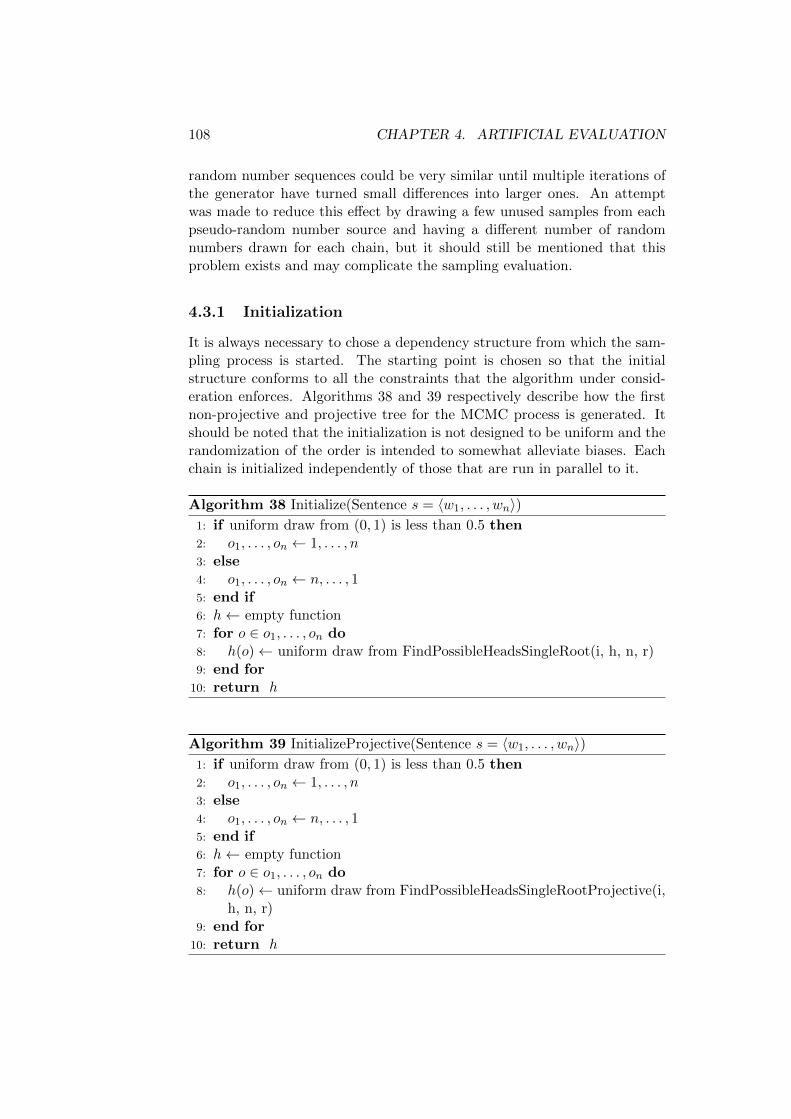
108 CHAPTER 4. ARTIFICIAL EVALUATION
random number sequences could be very similar until multiple iterations ofthe generator have turned small differences into larger ones. An attemptwas made to reduce this effect by drawing a few unused samples from eachpseudo-random number source and having a different number of randomnumbers drawn for each chain, but it should still be mentioned that thisproblem exists and may complicate the sampling evaluation.
4.3.1 Initialization
It is always necessary to chose a dependency structure from which the sam-pling process is started. The starting point is chosen so that the initialstructure conforms to all the constraints that the algorithm under consid-eration enforces. Algorithms 38 and 39 respectively describe how the firstnon-projective and projective tree for the MCMC process is generated. Itshould be noted that the initialization is not designed to be uniform and therandomization of the order is intended to somewhat alleviate biases. Eachchain is initialized independently of those that are run in parallel to it.
Algorithm 38 Initialize(Sentence s = 〈w1, . . . , wn〉)1: if uniform draw from (0, 1) is less than 0.5 then2: o1, . . . , on ← 1, . . . , n3: else4: o1, . . . , on ← n, . . . , 15: end if6: h← empty function7: for o ∈ o1, . . . , on do8: h(o)← uniform draw from FindPossibleHeadsSingleRoot(i, h, n, r)9: end for
10: return h
Algorithm 39 InitializeProjective(Sentence s = 〈w1, . . . , wn〉)1: if uniform draw from (0, 1) is less than 0.5 then2: o1, . . . , on ← 1, . . . , n3: else4: o1, . . . , on ← n, . . . , 15: end if6: h← empty function7: for o ∈ o1, . . . , on do8: h(o)← uniform draw from FindPossibleHeadsSingleRootProjective(i,
h, n, r)9: end for
10: return h
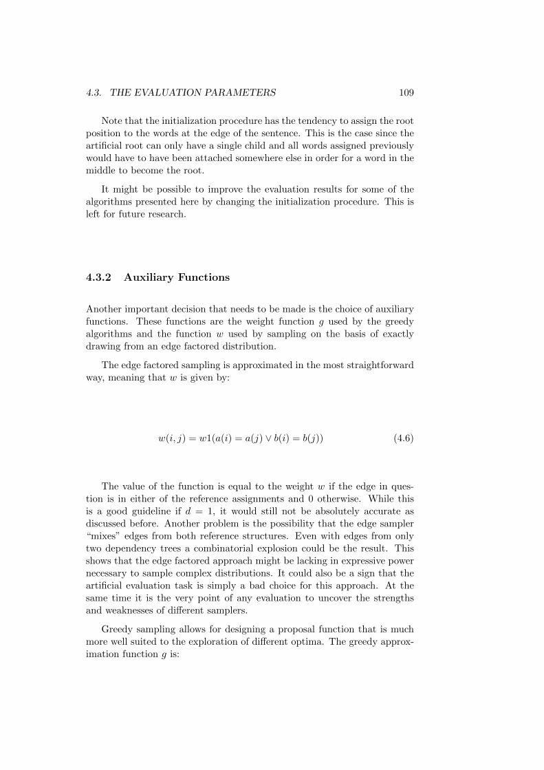
4.3. THE EVALUATION PARAMETERS 109
Note that the initialization procedure has the tendency to assign the rootposition to the words at the edge of the sentence. This is the case since theartificial root can only have a single child and all words assigned previouslywould have to have been attached somewhere else in order for a word in themiddle to become the root.
It might be possible to improve the evaluation results for some of thealgorithms presented here by changing the initialization procedure. This isleft for future research.
4.3.2 Auxiliary Functions
Another important decision that needs to be made is the choice of auxiliaryfunctions. These functions are the weight function g used by the greedyalgorithms and the function w used by sampling on the basis of exactlydrawing from an edge factored distribution.
The edge factored sampling is approximated in the most straightforwardway, meaning that w is given by:
w(i, j) = w1(a(i) = a(j) ∨ b(i) = b(j)) (4.6)
The value of the function is equal to the weight w if the edge in ques-tion is in either of the reference assignments and 0 otherwise. While thisis a good guideline if d = 1, it would still not be absolutely accurate asdiscussed before. Another problem is the possibility that the edge sampler“mixes” edges from both reference structures. Even with edges from onlytwo dependency trees a combinatorial explosion could be the result. Thisshows that the edge factored approach might be lacking in expressive powernecessary to sample complex distributions. It could also be a sign that theartificial evaluation task is simply a bad choice for this approach. At thesame time it is the very point of any evaluation to uncover the strengthsand weaknesses of different samplers.
Greedy sampling allows for designing a proposal function that is muchmore well suited to the exploration of different optima. The greedy approx-imation function g is:
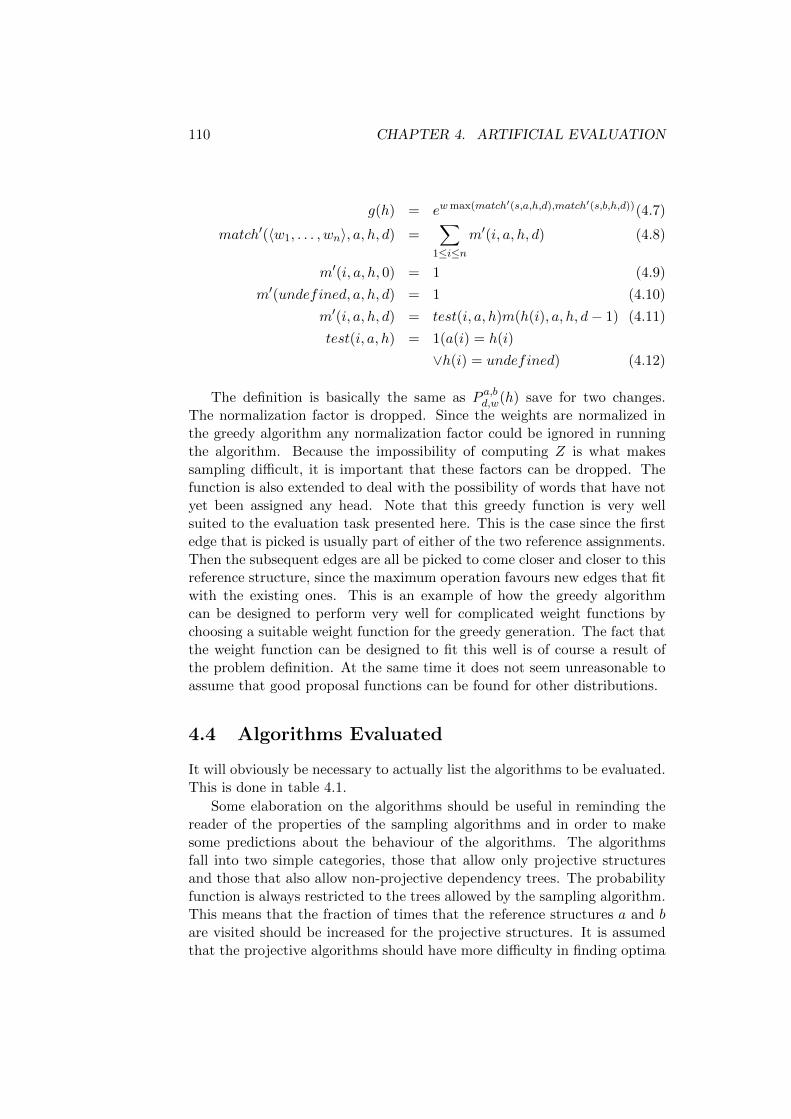
110 CHAPTER 4. ARTIFICIAL EVALUATION
g(h) = ew max(match′(s,a,h,d),match′(s,b,h,d))(4.7)
match′(〈w1, . . . , wn〉, a, h, d) =∑
1≤i≤nm′(i, a, h, d) (4.8)
m′(i, a, h, 0) = 1 (4.9)
m′(undefined, a, h, d) = 1 (4.10)
m′(i, a, h, d) = test(i, a, h)m(h(i), a, h, d− 1) (4.11)
test(i, a, h) = 1(a(i) = h(i)
∨h(i) = undefined) (4.12)
The definition is basically the same as P a,bd,w(h) save for two changes.
The normalization factor is dropped. Since the weights are normalized inthe greedy algorithm any normalization factor could be ignored in runningthe algorithm. Because the impossibility of computing Z is what makessampling difficult, it is important that these factors can be dropped. Thefunction is also extended to deal with the possibility of words that have notyet been assigned any head. Note that this greedy function is very wellsuited to the evaluation task presented here. This is the case since the firstedge that is picked is usually part of either of the two reference assignments.Then the subsequent edges are all be picked to come closer and closer to thisreference structure, since the maximum operation favours new edges that fitwith the existing ones. This is an example of how the greedy algorithmcan be designed to perform very well for complicated weight functions bychoosing a suitable weight function for the greedy generation. The fact thatthe weight function can be designed to fit this well is of course a result ofthe problem definition. At the same time it does not seem unreasonable toassume that good proposal functions can be found for other distributions.
4.4 Algorithms Evaluated
It will obviously be necessary to actually list the algorithms to be evaluated.This is done in table 4.1.
Some elaboration on the algorithms should be useful in reminding thereader of the properties of the sampling algorithms and in order to makesome predictions about the behaviour of the algorithms. The algorithmsfall into two simple categories, those that allow only projective structuresand those that also allow non-projective dependency trees. The probabilityfunction is always restricted to the trees allowed by the sampling algorithm.This means that the fraction of times that the reference structures a and bare visited should be increased for the projective structures. It is assumedthat the projective algorithms should have more difficulty in finding optima

4.4. ALGORITHMS EVALUATED 111
Abbreviation Number Short Description
MHProj 17 Sampling by proposing head assign-ments uniformly from a list of op-tions that do not violate the projec-tivity constraint. Root can be ex-changed for its left and right child.
GibbsProj 18 Sampling head assignments in aGibbs step from a list of options thatdo not violate the projectivity con-straint. Root can be exchanged forits left and right child.
GreedyProj 37 Combination of algorithm 18 andGreedy construction of a proposal.
MH 10 Sampling by proposing head assign-ments uniformly from a list of op-tions that do not violate the restric-tion to trees. Attempts are madeto randomly exchange the root forother words.
Gibbs 12 Sampling head assignments in aGibbs step from a list of optionsthat do not violate the constraintto trees. Each word is proposed asroot in turn and position to moveold root to is determined in a Gibbslike step.
Greedy 31 Uses algorithm 12 but replaces rootsampling with a greedy step.
Edge 22 Combines algorithm 12 with thesampling of the complete structurethrough the edge factored approach.
GreedyEdge 32 Uses algorithm 12 but replaces rootsampling with a greedy step. Alsoadds an edge factored samplingstep.
Figure 4.1: This table lists the different algorithms evaluated along withthe abbreviations used to refer to them in the text. For each algorithm thenumber it has in the text is given. There is also a short description as areminder of the way the algorithm works.
112 CHAPTER 4. ARTIFICIAL EVALUATION
and moving between them. This is the case since the possible moves in non-global algorithms are more restricted when no crossing edges are allowed.
The projective restriction is enforced by algorithms 17, 18 and 37. Thefirst algorithm is the least resource intensive and it is based on local search.The behaviour one would expect is that sooner or later the uniform proposalsfor the heads of single words lead to one of the two reference assignments.This is the case since moves towards structures with greater probabilityare always accept by the sampler. This is true with the exception of theroot sampling step which has a small correction factor. Unless w is chosento be very small, the weight will most likely be offset by the probabilityfunction. Once a good assignment has been found, the movement of thechain constructed from algorithm 17 should then most likely get stuck inthe vicinity of assignment because of the strictly local moves. This meansthat it can be expected that the sampling algorithm performs poorly unlessboth reference structures are very similar, a large number of parallel chainsis used or the weight is very small. The same would be true for algorithm18. The main difference is the fact that all proposals are computed bytaking the weights of the assignments that would result. This means thatthe behaviour is similar to algorithm 17 except that the discovery of one ofthe reference structures will be quicker. Finally algorithm 37 extends theGibbs based approach by a greedy global approach. The expectation is thatthis algorithm converges fast and moves between the different optima.
t can also be expected for algorithms 18 and 37 that they use much moreevaluations of the probability function. These are made during the Gibbssteps. The greedy step adds only two evaluations of the target function. Itdoes however add a large number of evaluations of the auxiliary function g.This function will be almost as costly as the actual probability. It shouldtherefore be kept in mind that there is a substantial cost increase for thegreedy sampling step. The combination of Gibbs sampling and greedy sam-pling is chosen to explore the settings close to the proposals made by thegreedy sampler.
The other algorithms all allow for non-projective dependency structures.The expectation would be that, since they can move more freely, they shouldbe able to find optima more easily. At the same time there is a larger spacethat needs to be explored which could be problematic for algorithm 10. Thisis the cheapest of the non-projective samplers. Algorithm 12 costs more sincethe proposals are once again made based on the probability function. Fromthis one could also once again assume that the time to reach one of thereference structures is reduced. Algorithm 22 adds an additional step thatis cheap in in terms of probability function evaluations but requires a num-ber of evaluations of the auxiliary function. The addition of a global stepin this case may help with convergence, but since the global step is basedon a very weak approximation of the actual function it may not contributemuch in case of a higher d value. The greedy algorithm 31 is even costlier
4.5. STATISTICS USED 113
in terms of auxiliary evaluations, since it has a more complex approxima-tion function but it is reasonable to expect the algorithm to perform wellprecisely because it makes use of this additional source of information. Thelast technique evaluated is also the most costly. Both of the global tech-niques are combined in algorithm 32 and one hopes that the high demand incomputational resources pays of in terms of good performance in estimatingquantities of interest.
4.5 Statistics Used
The final topic that needs to be discussed before the actual evaluation resultscan be presented are the exact definitions of the statistics kept. While mostof these have been mentioned before, this section attempts to reduce allpossible ambiguities to a minimum. Note that when the results are graphedlater in this chapter each data point is taken as a sum over all chains insteadof attempting to find a single “representative” chain’s performance to plot.
4.5.1 Ratio of Reference Assignments
The main statistic is the ratio of the samples that are equal to trees a andb respectively. Statistics similar to this one may be useful for different tasksin NLP. An obvious application of such ratios would be to decide whichassignment to return as the “better” one among a number of choices. Thiscould be the one more likely according to the sample and if the ratios arecomputed correctly, then they would represent a difference in the weight as-signed by the model. It would also be possible to make use of the minimumrisk approach to parsing and use the ratios to select single edges [6, 48].Another possible application that needs the relative frequency with whichcertain features of the input are expected would be the training of Condi-tional Random Fields with stochastic gradient descent [60, 114, 35, 112].The ratio also has the advantage of being a feature of a distribution thatcan be predicted analytically with greater ease than measures that take intoconsideration others aspects of the sample. Another reason that a ratio isinteresting is the fact that it focuses the evaluation on values that have highprobability in the target distribution and are therefore likely to be exploredearly in the MCMC process.
The actual value used is the median among all 100 times the experimentis repeated of max( seenit(a)
seenit(b), seenit(b)seenit(a)). The values seenit(x) denote how many
times x was among the observations generated up to iteration it. The medianamong the different repetitions means that the values for 100 repetitions arecomputed from the different chains seen in each repetition of the experiment.The values from different runs are then ordered from smallest to largest andthe middle value in this list is chosen. Due to rounding down, this wouldbe the entry number 50 counting from 1. Note that, because the Java [37]
114 CHAPTER 4. ARTIFICIAL EVALUATION
ordering of double precision floating point numbers was used, NotANumberis moved to the end of this list. The median is chosen since the value willbe infinity for at least some repetitions of the experiment in which onlyone of the reference trees is found and this would change the value of anymean to infinity. If the median is less then infinity, then this would meanthat at least half of the times the sampler “found” both modes in at leastsome of the parallel chains. If the value is close to 1.0, then this wouldmean that the MCMC algorithm more or less correctly models the relativelikelihood of the two assignments with the samples generated up to thatstep. The maximum of two fractions is used in order to make deviationsmore readily interpretable. It implies that values are always in the rangefrom 1.0 upwards. If it was just a fraction of the form seenit(a)
seenit(b), then the
values would simply vary between 0 and 1 if there was a tendency to producemore observations of b than of a and vary between 1.0 and infinity in theopposite case. The restriction to values from 1.0 upwards also means that itis possible to express situations in which neither of the structures have beenfound -resulting in a value of NaN- by the value 0.
4.5.2 The Third Quartile
The third quartile for the values of max( seenit(a)seenit(b)
, seenit(b)seenit(a)) is also reported.
The concept is basically the one introduced in the previous subsection exceptthat the last of the first three quarters of values is used instead of the last ofthe first half. This extension is used to expand information on the robustnessof the MCMC scheme. This statistic has a better chance to reach a muchlarger value of the fraction and will therefore be a more pessimistic estimatethan the median value. This also means that it is more likely that algorithmbehave at least as well as suggest by this value.
4.5.3 Count of Reference Assignments
Both the averages over the values seenit(a) and seenit(b) are tracked for allexperiments. If there are n chains run in parallel, then this value reportshow often the algorithm for sampling has returned a or b in each of the nparallel chains up to iteration it. The value either increases or stays thesame for every iteration taken. Unless the algorithm is biased in favour ofeither a or b it would be expected that the average over all repetitions of theexperiment is about the same for a and b. The reverse of this implies thatan imbalance in this estimate indicates some bias in the algorithm and theyway it is initialized. Note that these biases are possible in MCMC schemes,they simply average out after sufficient runtime.
4.6. EVALUATION RESULTS 115
4.5.4 Function Evaluations
The averages over all repetitions of the probability function evaluations aretracked. The number is summed up when multiple sampling algorithms arerun in parallel, the value is summed up for all chains, therefore the increasedcost of using multiple chains is reflected. It is desirable to compare the costof this function to the cost of evaluating auxiliary functions. The cheapestauxiliary function is the edge factored function w that is only evaluated on asingle edge. In order to make the values comparable the counts of the timesthe probability function has been evaluated will be multiplied by the lengthof the dependency structure on which a sampler is used. It would be easyto recover the original value by dividing accordingly. As a result the valuereflects the number of edges that have been considered in the computationof the probability function, ignoring the fact that some iteration over thedependencies proportional to the factor d will be necessary. As stated before,the function is the main indicator of the computational resources that haveto be dedicated in order to use a certain algorithm.
4.5.5 Auxiliary Function Evaluations
In addition to the number of times the probability function was evaluatedthe same number is presented for the auxiliary functions for greedy andand edge factored sampling. Once again an average is used over all therepetitions of the sampling process and the uses of the function are summedfor multiple chains. The auxiliary function only inspects single edges andis therefore not scaled in any way. The greedy function on the other handinspects every edge in a structure1. Therefore is it also scaled by the lengthof the dependency structure. If both functions are used, then the number ofauxiliary evaluations is the sum of the evaluations made for both functionswith the greedy one scaled and the auxiliary one unscaled.
4.6 Evaluation Results
In this section presents the actual evaluation results, first with some ex-periments in which the single root sampling aspect will have less influence,because the two reference structures will have the same word attached to theartificial root. This means that once the root has been found one can expectany sampler, as long as w is set high enough, to have little problem to stickwith this root and the sampling problem is focused on going through the dif-ferent structures that have this root node. After a good number of insightshave been gleaned from evaluation on this reduced problem, the evaluationis extended to structures with differing root positions. The first evaluationis extensive in order to give an impression of the different strengths and
1Or notes that there is no edge for certain words.
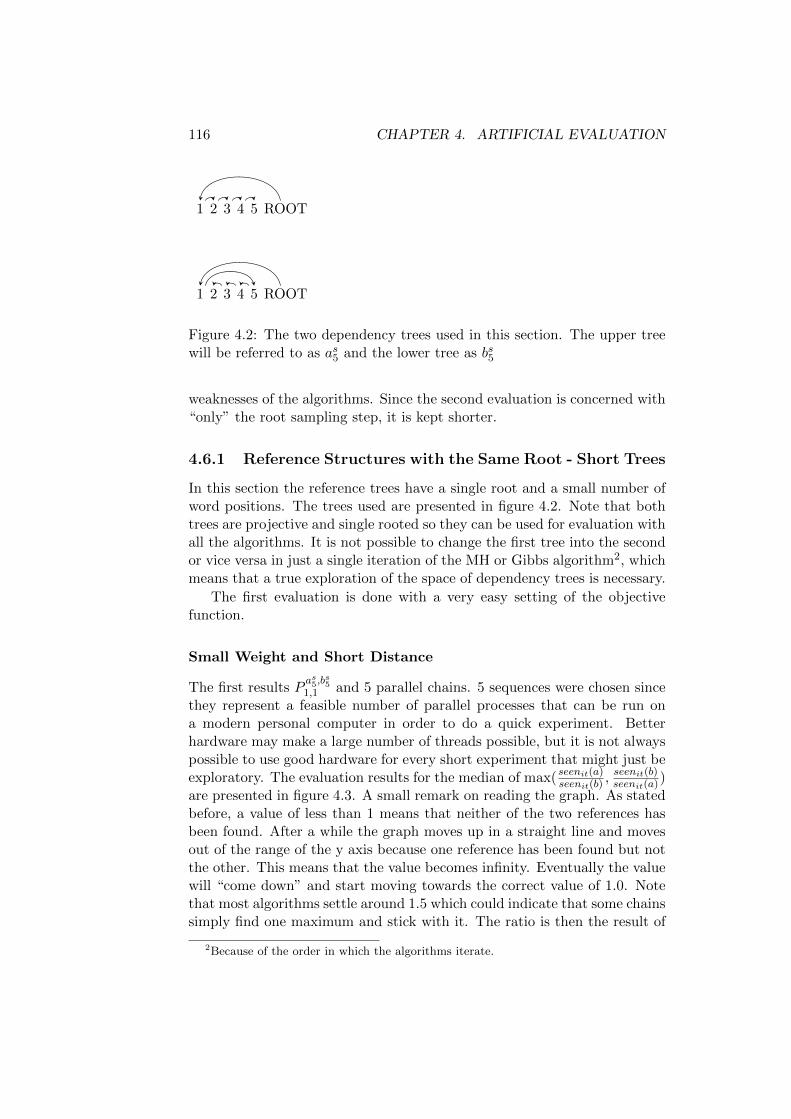
116 CHAPTER 4. ARTIFICIAL EVALUATION
1 2 3 4 5 ROOT
1 2 3 4 5 ROOT
Figure 4.2: The two dependency trees used in this section. The upper treewill be referred to as as5 and the lower tree as bs5
weaknesses of the algorithms. Since the second evaluation is concerned with“only” the root sampling step, it is kept shorter.
4.6.1 Reference Structures with the Same Root - Short Trees
In this section the reference trees have a single root and a small number ofword positions. The trees used are presented in figure 4.2. Note that bothtrees are projective and single rooted so they can be used for evaluation withall the algorithms. It is not possible to change the first tree into the secondor vice versa in just a single iteration of the MH or Gibbs algorithm2, whichmeans that a true exploration of the space of dependency trees is necessary.
The first evaluation is done with a very easy setting of the objectivefunction.
Small Weight and Short Distance
The first results Pas5,b
s5
1,1 and 5 parallel chains. 5 sequences were chosen sincethey represent a feasible number of parallel processes that can be run ona modern personal computer in order to do a quick experiment. Betterhardware may make a large number of threads possible, but it is not alwayspossible to use good hardware for every short experiment that might just beexploratory. The evaluation results for the median of max( seenit(a)
seenit(b), seenit(b)seenit(a))
are presented in figure 4.3. A small remark on reading the graph. As statedbefore, a value of less than 1 means that neither of the two references hasbeen found. After a while the graph moves up in a straight line and movesout of the range of the y axis because one reference has been found but notthe other. This means that the value becomes infinity. Eventually the valuewill “come down” and start moving towards the correct value of 1.0. Notethat most algorithms settle around 1.5 which could indicate that some chainssimply find one maximum and stick with it. The ratio is then the result of
2Because of the order in which the algorithms iterate.
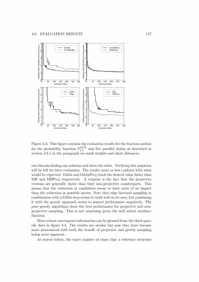
4.6. EVALUATION RESULTS 117
GreedyGreedyEdge
Med
ian
Rati
o O
f Ref
eren
ce S
truc
ture
s
0
1
2
3
4
5
Iteration Steps0 50 100 150 200 250 300
GreedyProjGibbsProj
Med
ian
Rati
o O
f Ref
eren
ce S
truc
ture
s0
1
2
3
4
5
Iteration Steps0 50 100 150 200 250 300
GibbsEdge
Med
ian
Rati
o O
f Ref
eren
ce S
truc
ture
s
0
1
2
3
4
5
Iteration Steps0 50 100 150 200 250 300
MHMHProj
Med
ian
Rati
o O
f Ref
eren
ce S
truc
ture
s
0
1
2
3
4
5
Iteration Steps0 50 100 150 200 250 300
Figure 4.3: This figure contains the evaluation results for the fraction median
for the probability function Pas5,b
s5
1,1 and five parallel chains as described insection 4.6.1 in the paragraph on small weights and short distances.
two threads finding one solution and three the other. Verifying this suspicionwill be left for later evaluation. The results more or less conform with whatwould be expected. Gibbs and GibbsProj reach the desired value faster thanMH and MHProj respectively. A surprise is the fact that the projectiveversions are generally faster than their non-projective counterparts. Thismeans that the reduction in candidates seems to have more of an impactthan the reduction in possible moves. Note that edge factored sampling incombination with a Gibbs step seems to work well on its own, but combiningit with the greedy approach seems to impact performance negatively. Thepure greedy algorithms show the best performance for projective and non-projective sampling. This is not surprising given the well suited auxiliaryfunction.
More robust convergence information can be gleaned from the third quar-tile data in figure 4.4. The results are similar but now they have becomemore pronounced with both the benefit of projective and greedy samplingbeing more apparent.
As stated before, the exact number of times that a reference structure

118 CHAPTER 4. ARTIFICIAL EVALUATION
GreedyGreedyEdge
Thir
d Q
uart
ile R
atio
Of R
efer
ence
Str
uctu
res
0
1
2
3
4
5
Iteration Steps0 50 100 150 200 250 300
GreedyProjGibbsProj
Thir
d Q
uart
ile R
atio
Of R
efer
ence
Str
uctu
res
0
1
2
3
4
5
Iteration Steps0 50 100 150 200 250 300
GibbsEdge
Thir
d Q
uart
ile R
atio
Of R
efer
ence
Str
uctu
res
0
1
2
3
4
5
Iteration Steps0 50 100 150 200 250 300
MHMHProj
Thir
d Q
uart
ile R
atio
Of R
efer
ence
Str
uctu
res
0
1
2
3
4
5
Iteration Steps0 50 100 150 200 250 300
Figure 4.4: This figure contains the evaluation results for the fraction third
quartile for the probability function Pas5,b
s5
1,1 and five parallel chains as de-scribed in section 4.6.1 in the paragraph on small weights and short dis-tances.
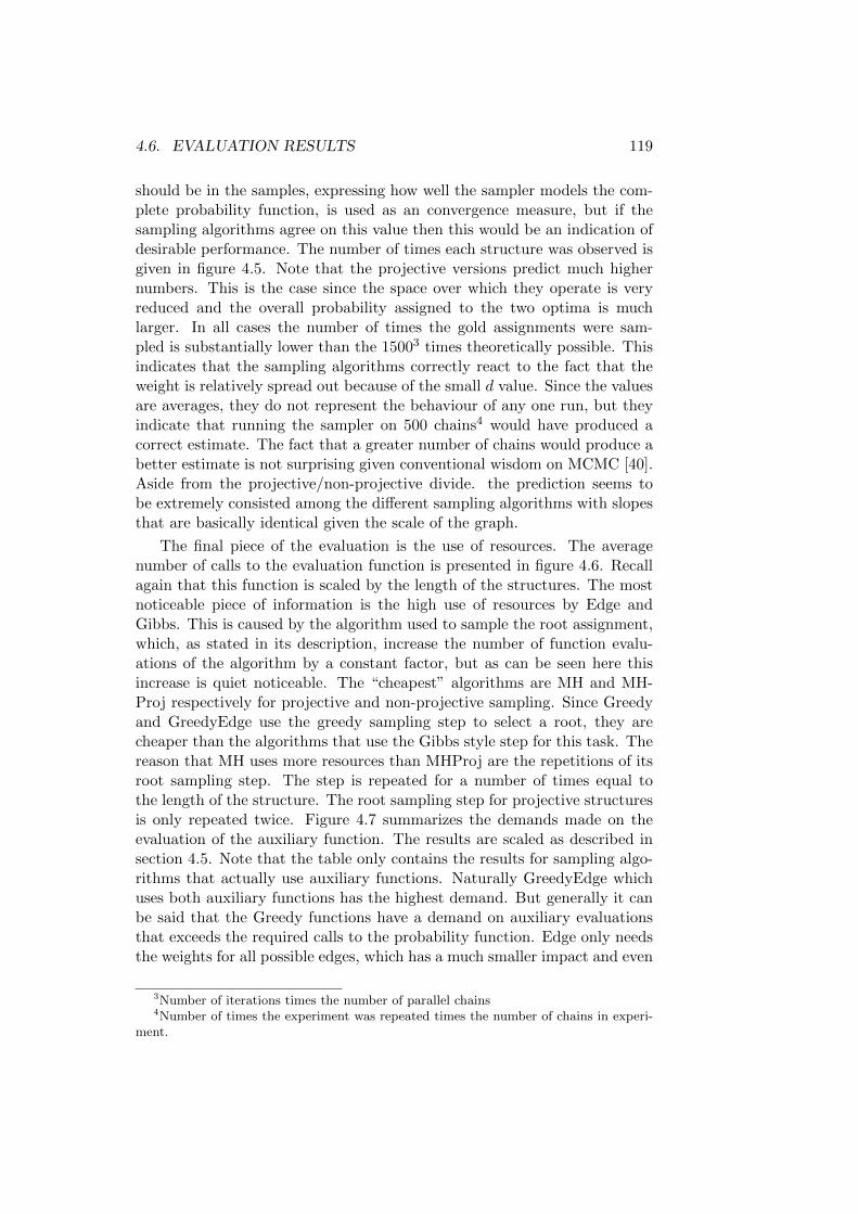
4.6. EVALUATION RESULTS 119
should be in the samples, expressing how well the sampler models the com-plete probability function, is used as an convergence measure, but if thesampling algorithms agree on this value then this would be an indication ofdesirable performance. The number of times each structure was observed isgiven in figure 4.5. Note that the projective versions predict much highernumbers. This is the case since the space over which they operate is veryreduced and the overall probability assigned to the two optima is muchlarger. In all cases the number of times the gold assignments were sam-pled is substantially lower than the 15003 times theoretically possible. Thisindicates that the sampling algorithms correctly react to the fact that theweight is relatively spread out because of the small d value. Since the valuesare averages, they do not represent the behaviour of any one run, but theyindicate that running the sampler on 500 chains4 would have produced acorrect estimate. The fact that a greater number of chains would produce abetter estimate is not surprising given conventional wisdom on MCMC [40].Aside from the projective/non-projective divide. the prediction seems tobe extremely consisted among the different sampling algorithms with slopesthat are basically identical given the scale of the graph.
The final piece of the evaluation is the use of resources. The averagenumber of calls to the evaluation function is presented in figure 4.6. Recallagain that this function is scaled by the length of the structures. The mostnoticeable piece of information is the high use of resources by Edge andGibbs. This is caused by the algorithm used to sample the root assignment,which, as stated in its description, increase the number of function evalu-ations of the algorithm by a constant factor, but as can be seen here thisincrease is quiet noticeable. The “cheapest” algorithms are MH and MH-Proj respectively for projective and non-projective sampling. Since Greedyand GreedyEdge use the greedy sampling step to select a root, they arecheaper than the algorithms that use the Gibbs style step for this task. Thereason that MH uses more resources than MHProj are the repetitions of itsroot sampling step. The step is repeated for a number of times equal tothe length of the structure. The root sampling step for projective structuresis only repeated twice. Figure 4.7 summarizes the demands made on theevaluation of the auxiliary function. The results are scaled as described insection 4.5. Note that the table only contains the results for sampling algo-rithms that actually use auxiliary functions. Naturally GreedyEdge whichuses both auxiliary functions has the highest demand. But generally it canbe said that the Greedy functions have a demand on auxiliary evaluationsthat exceeds the required calls to the probability function. Edge only needsthe weights for all possible edges, which has a much smaller impact and even
3Number of iterations times the number of parallel chains4Number of times the experiment was repeated times the number of chains in experi-
ment.

120 CHAPTER 4. ARTIFICIAL EVALUATION
GreedyGreedyEdge
Seen
(a)
0
20
40
60
80
100
Iteration Steps0 50 100 150 200 250 300
GreedyProjGibbsProj
Seen
(a)
0
20
40
60
80
100
Iteration Steps0 50 100 150 200 250 300
GibbsEdge
Seen
(a)
0
20
40
60
80
100
Iteration Steps0 50 100 150 200 250 300
MHMHProj
Seen
(a)
0
20
40
60
80
100
Iteration Steps0 50 100 150 200 250 300
GreedyGreedyEdge
Seen
(b)
0
20
40
60
80
100
Iteration Steps0 50 100 150 200 250 300
GreedyProjGibbsProj
Seen
(b)
0
20
40
60
80
100
Iteration Steps0 50 100 150 200 250 300
GibbsEdge
Seen
(b)
0
20
40
60
80
100
Iteration Steps0 50 100 150 200 250 300
MHMHProj
Seen
(b)
0
20
40
60
80
100
Iteration Steps0 50 100 150 200 250 300
Figure 4.5: This figure contains the number of times that each reference tree
was seen during sampling for the probability function Pas5,b
s5
1,1 and five parallelchains as described in section 4.6.1 in the paragraph on small weights andshort distances. The upper figure shows the value for structure as5 and thelower for bs5.
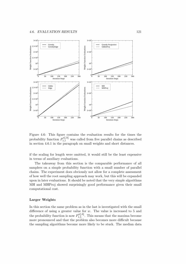
4.6. EVALUATION RESULTS 121
GreedyGreedyEdge
Wei
ght F
unct
ion
Eval
uati
ons
0
5×10⁴
105
1.5×10⁵
2×10⁵
2.5×10⁵
3×10⁵
Iteration Steps0 50 100 150 200 250 300
Greedy ProjectiveGibbsProj
Wei
ght F
unct
ion
Eval
uati
ons
0
5×10⁴
105
2×10⁵
3×10⁵
Iteration Steps0 50 100 150 200 250 300
GibbsEdge
Wei
ght F
unct
ion
Eval
uati
ons
0
5×10⁴
105
1.5×10⁵
2×10⁵
2.5×10⁵
3×10⁵
Iteration Steps0 50 100 150 200 250 300
MHMHProj
Wei
ght F
unct
ion
Eval
uati
ons
0
5×10⁴
105
2×10⁵
3×10⁵
Iteration Steps0 50 100 150 200 250 300
Figure 4.6: This figure contains the evaluation results for the times the
probability function Pas5,b
s5
1,1 was called from five parallel chains as describedin section 4.6.1 in the paragraph on small weights and short distances.
if the scaling for length were omitted, it would still be the least expensivein terms of auxiliary evaluations.
The takeaway from this section is the comparable performance of allsamplers on a simple probability function with a small number of parallelchains. The experiment does obviously not allow for a complete assessmentof how well the root sampling approach may work, but this will be expandedupon in later evaluations. It should be noted that the very simple algorithmsMH and MHProj showed surprisingly good performance given their smallcomputational cost.
Larger Weights
In this section the same problem as in the last is investigated with the smalldifference of using a greater value for w. The value is increased to 5 and
the probability function is now Pas5,b
s5
1,5 . This means that the maxima becomemore pronounced and that the problem also becomes more difficult becausethe sampling algorithms become more likely to be stuck. The median data
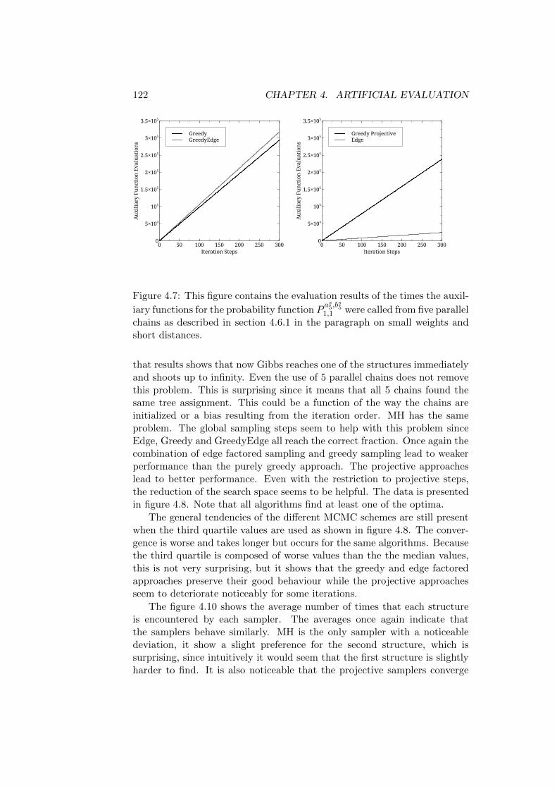
122 CHAPTER 4. ARTIFICIAL EVALUATION
GreedyGreedyEdge
Aux
iliar
y Fu
ncti
on E
valu
atio
ns
0
5×10⁴
105
1.5×10⁵
2×10⁵
2.5×10⁵
3×10⁵
3.5×10⁵
Iteration Steps0 50 100 150 200 250 300
Greedy ProjectiveEdge
Aux
iliar
y Fu
ncti
on E
valu
atio
ns
0
5×10⁴
105
1.5×10⁵
2×10⁵
2.5×10⁵
3×10⁵
3.5×10⁵
Iteration Steps0 50 100 150 200 250 300
Figure 4.7: This figure contains the evaluation results of the times the auxil-
iary functions for the probability function Pas5,b
s5
1,1 were called from five parallelchains as described in section 4.6.1 in the paragraph on small weights andshort distances.
that results shows that now Gibbs reaches one of the structures immediatelyand shoots up to infinity. Even the use of 5 parallel chains does not removethis problem. This is surprising since it means that all 5 chains found thesame tree assignment. This could be a function of the way the chains areinitialized or a bias resulting from the iteration order. MH has the sameproblem. The global sampling steps seem to help with this problem sinceEdge, Greedy and GreedyEdge all reach the correct fraction. Once again thecombination of edge factored sampling and greedy sampling lead to weakerperformance than the purely greedy approach. The projective approacheslead to better performance. Even with the restriction to projective steps,the reduction of the search space seems to be helpful. The data is presentedin figure 4.8. Note that all algorithms find at least one of the optima.
The general tendencies of the different MCMC schemes are still presentwhen the third quartile values are used as shown in figure 4.8. The conver-gence is worse and takes longer but occurs for the same algorithms. Becausethe third quartile is composed of worse values than the the median values,this is not very surprising, but it shows that the greedy and edge factoredapproaches preserve their good behaviour while the projective approachesseem to deteriorate noticeably for some iterations.
The figure 4.10 shows the average number of times that each structureis encountered by each sampler. The averages once again indicate thatthe samplers behave similarly. MH is the only sampler with a noticeabledeviation, it show a slight preference for the second structure, which issurprising, since intuitively it would seem that the first structure is slightlyharder to find. It is also noticeable that the projective samplers converge

4.6. EVALUATION RESULTS 123
GreedyGreedyEdge
Med
ian
Rati
o O
f Ref
eren
ce S
truc
ture
s
0
1
2
3
4
5
Iteration Steps0 50 100 150 200 250 300
GreedyProjGibbsProj
Med
ian
Rati
o O
f Ref
eren
ce S
truc
ture
s
0
1
2
3
4
5
Iteration Steps0 50 100 150 200 250 300
GibbsEdge
Med
ian
Rati
o O
f Ref
eren
ce S
truc
ture
s
0
1
2
3
4
5
Iteration Steps0 50 100 150 200 250 300
MHMHProj
Med
ian
Rati
o O
f Ref
eren
ce S
truc
ture
s
0
1
2
3
4
5
Iteration Steps0 50 100 150 200 250 300
Figure 4.8: This figure contains the evaluation results for the fraction median
for the probability function Pas5,b
s5
1,5 and five parallel chains as described insection 4.6.1 in the paragraph on increased weights.
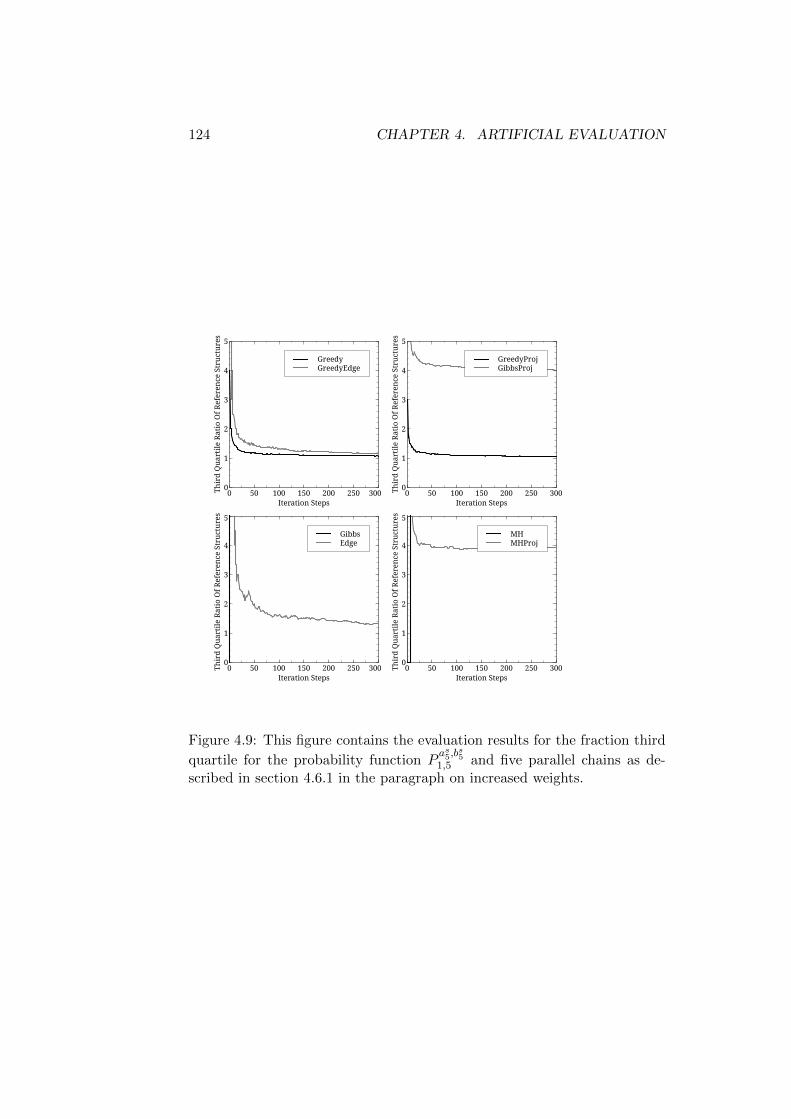
124 CHAPTER 4. ARTIFICIAL EVALUATION
GreedyGreedyEdge
Thir
d Q
uart
ile R
atio
Of R
efer
ence
Str
uctu
res
0
1
2
3
4
5
Iteration Steps0 50 100 150 200 250 300
GreedyProjGibbsProj
Thir
d Q
uart
ile R
atio
Of R
efer
ence
Str
uctu
res
0
1
2
3
4
5
Iteration Steps0 50 100 150 200 250 300
GibbsEdge
Thir
d Q
uart
ile R
atio
Of R
efer
ence
Str
uctu
res
0
1
2
3
4
5
Iteration Steps0 50 100 150 200 250 300
MHMHProj
Thir
d Q
uart
ile R
atio
Of R
efer
ence
Str
uctu
res
0
1
2
3
4
5
Iteration Steps0 50 100 150 200 250 300
Figure 4.9: This figure contains the evaluation results for the fraction third
quartile for the probability function Pas5,b
s5
1,5 and five parallel chains as de-scribed in section 4.6.1 in the paragraph on increased weights.
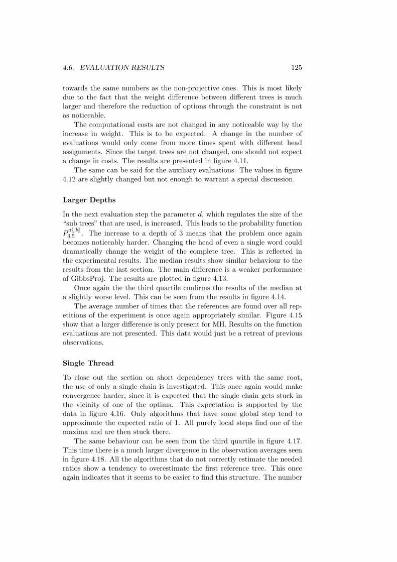
4.6. EVALUATION RESULTS 125
towards the same numbers as the non-projective ones. This is most likelydue to the fact that the weight difference between different trees is muchlarger and therefore the reduction of options through the constraint is notas noticeable.
The computational costs are not changed in any noticeable way by theincrease in weight. This is to be expected. A change in the number ofevaluations would only come from more times spent with different headassignments. Since the target trees are not changed, one should not expecta change in costs. The results are presented in figure 4.11.
The same can be said for the auxiliary evaluations. The values in figure4.12 are slightly changed but not enough to warrant a special discussion.
Larger Depths
In the next evaluation step the parameter d, which regulates the size of the“sub trees” that are used, is increased. This leads to the probability function
Pas5,b
s5
3,5 . The increase to a depth of 3 means that the problem once againbecomes noticeably harder. Changing the head of even a single word coulddramatically change the weight of the complete tree. This is reflected inthe experimental results. The median results show similar behaviour to theresults from the last section. The main difference is a weaker performanceof GibbsProj. The results are plotted in figure 4.13.
Once again the the third quartile confirms the results of the median ata slightly worse level. This can be seen from the results in figure 4.14.
The average number of times that the references are found over all rep-etitions of the experiment is once again appropriately similar. Figure 4.15show that a larger difference is only present for MH. Results on the functionevaluations are not presented. This data would just be a retreat of previousobservations.
Single Thread
To close out the section on short dependency trees with the same root,the use of only a single chain is investigated. This once again would makeconvergence harder, since it is expected that the single chain gets stuck inthe vicinity of one of the optima. This expectation is supported by thedata in figure 4.16. Only algorithms that have some global step tend toapproximate the expected ratio of 1. All purely local steps find one of themaxima and are then stuck there.
The same behaviour can be seen from the third quartile in figure 4.17.This time there is a much larger divergence in the observation averages seenin figure 4.18. All the algorithms that do not correctly estimate the neededratios show a tendency to overestimate the first reference tree. This onceagain indicates that it seems to be easier to find this structure. The number
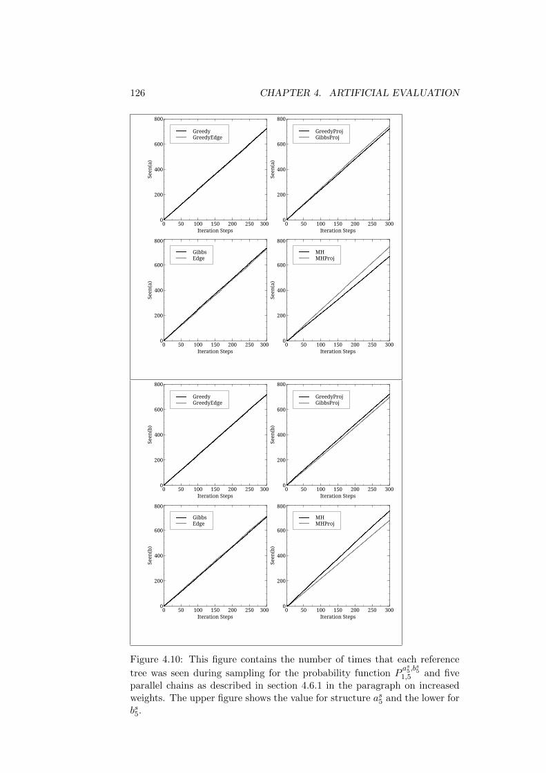
126 CHAPTER 4. ARTIFICIAL EVALUATION
GreedyGreedyEdge
Seen
(a)
0
200
400
600
800
Iteration Steps0 50 100 150 200 250 300
GreedyProjGibbsProj
Seen
(a)
0
200
400
600
800
Iteration Steps0 50 100 150 200 250 300
GibbsEdge
Seen
(a)
0
200
400
600
800
Iteration Steps0 50 100 150 200 250 300
MHMHProj
Seen
(a)
0
200
400
600
800
Iteration Steps0 50 100 150 200 250 300
GreedyGreedyEdge
Seen
(b)
0
200
400
600
800
Iteration Steps0 50 100 150 200 250 300
GreedyProjGibbsProj
Seen
(b)
0
200
400
600
800
Iteration Steps0 50 100 150 200 250 300
GibbsEdge
Seen
(b)
0
200
400
600
800
Iteration Steps0 50 100 150 200 250 300
MHMHProj
Seen
(b)
0
200
400
600
800
Iteration Steps0 50 100 150 200 250 300
Figure 4.10: This figure contains the number of times that each reference
tree was seen during sampling for the probability function Pas5,b
s5
1,5 and fiveparallel chains as described in section 4.6.1 in the paragraph on increasedweights. The upper figure shows the value for structure as5 and the lower forbs5.
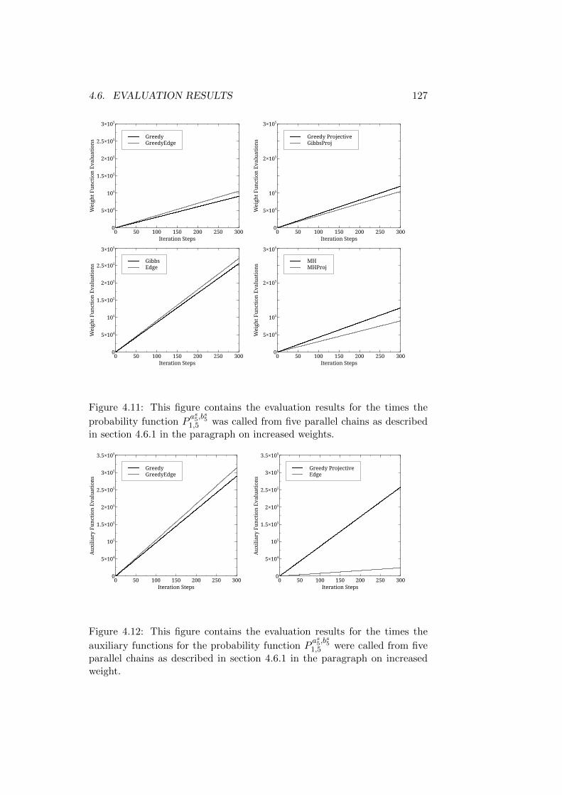
4.6. EVALUATION RESULTS 127
GreedyGreedyEdge
Wei
ght F
unct
ion
Eval
uati
ons
0
5×10⁴
105
1.5×10⁵
2×10⁵
2.5×10⁵
3×10⁵
Iteration Steps0 50 100 150 200 250 300
Greedy ProjectiveGibbsProj
Wei
ght F
unct
ion
Eval
uati
ons
0
5×10⁴
105
2×10⁵
3×10⁵
Iteration Steps0 50 100 150 200 250 300
GibbsEdge
Wei
ght F
unct
ion
Eval
uati
ons
0
5×10⁴
105
1.5×10⁵
2×10⁵
2.5×10⁵
3×10⁵
Iteration Steps0 50 100 150 200 250 300
MHMHProj
Wei
ght F
unct
ion
Eval
uati
ons
0
5×10⁴
105
2×10⁵
3×10⁵
Iteration Steps0 50 100 150 200 250 300
Figure 4.11: This figure contains the evaluation results for the times the
probability function Pas5,b
s5
1,5 was called from five parallel chains as describedin section 4.6.1 in the paragraph on increased weights.
GreedyGreedyEdge
Aux
iliar
y Fu
ncti
on E
valu
atio
ns
0
5×10⁴
105
1.5×10⁵
2×10⁵
2.5×10⁵
3×10⁵
3.5×10⁵
Iteration Steps0 50 100 150 200 250 300
Greedy ProjectiveEdge
Aux
iliar
y Fu
ncti
on E
valu
atio
ns
0
5×10⁴
105
1.5×10⁵
2×10⁵
2.5×10⁵
3×10⁵
3.5×10⁵
Iteration Steps0 50 100 150 200 250 300
Figure 4.12: This figure contains the evaluation results for the times the
auxiliary functions for the probability function Pas5,b
s5
1,5 were called from fiveparallel chains as described in section 4.6.1 in the paragraph on increasedweight.

128 CHAPTER 4. ARTIFICIAL EVALUATION
GreedyGreedyEdge
Med
ian
Rati
o O
f Ref
eren
ce S
truc
ture
s
0
1
2
3
4
5
Iteration Steps0 50 100 150 200 250 300
GreedyProjGibbsProj
Med
ian
Rati
o O
f Ref
eren
ce S
truc
ture
s
0
1
2
3
4
5
Iteration Steps0 50 100 150 200 250 300
GibbsEdge
Med
ian
Rati
o O
f Ref
eren
ce S
truc
ture
s
0
1
2
3
4
5
Iteration Steps0 50 100 150 200 250 300
MHMHProj
Med
ian
Rati
o O
f Ref
eren
ce S
truc
ture
s
0
1
2
3
4
5
Iteration Steps0 50 100 150 200 250 300
Figure 4.13: This figure contains the evaluation results for the fraction me-
dian for the probability function Pas5,b
s5
3,5 and five parallel chains as describedin section 4.6.1 in the paragraph on increased weights and depth.
4.6. EVALUATION RESULTS 129
GreedyGreedyEdge
Thir
d Q
uart
ile R
atio
Of R
efer
ence
Str
uctu
res
0
1
2
3
4
5
Iteration Steps0 50 100 150 200 250 300
GreedyProjGibbsProj
Thir
d Q
uart
ile R
atio
Of R
efer
ence
Str
uctu
res
0
1
2
3
4
5
Iteration Steps0 50 100 150 200 250 300
GibbsEdge
Thir
d Q
uart
ile R
atio
Of R
efer
ence
Str
uctu
res
0
1
2
3
4
5
Iteration Steps0 50 100 150 200 250 300
MHMHProj
Thir
d Q
uart
ile R
atio
Of R
efer
ence
Str
uctu
res
0
1
2
3
4
5
Iteration Steps0 50 100 150 200 250 300
Figure 4.14: This figure contains the evaluation results for the fraction third
quartile for the probability function Pas5,b
s5
3,5 and five parallel chains as de-scribed in section 4.6.1 in the paragraph on increased weights and depth.
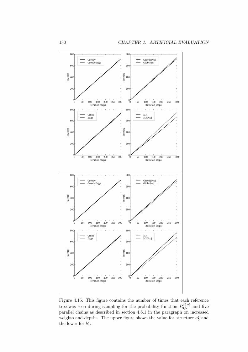
130 CHAPTER 4. ARTIFICIAL EVALUATION
GreedyGreedyEdge
Seen
(a)
0
200
400
600
800
Iteration Steps0 50 100 150 200 250 300
GreedyProjGibbsProj
Seen
(a)
0
200
400
600
800
Iteration Steps0 50 100 150 200 250 300
GibbsEdge
Seen
(a)
0
200
400
600
800
Iteration Steps0 50 100 150 200 250 300
MHMHProj
Seen
(a)
0
200
400
600
800
Iteration Steps0 50 100 150 200 250 300
GreedyGreedyEdge
Seen
(b)
0
200
400
600
800
Iteration Steps0 50 100 150 200 250 300
GreedyProjGibbsProj
Seen
(b)
0
200
400
600
800
Iteration Steps0 50 100 150 200 250 300
GibbsEdge
Seen
(b)
0
200
400
600
800
Iteration Steps0 50 100 150 200 250 300
MHMHProj
Seen
(b)
0
200
400
600
800
Iteration Steps0 50 100 150 200 250 300
Figure 4.15: This figure contains the number of times that each reference
tree was seen during sampling for the probability function Pas5,b
s5
3,5 and fiveparallel chains as described in section 4.6.1 in the paragraph on increasedweights and depths. The upper figure shows the value for structure as5 andthe lower for bs5.
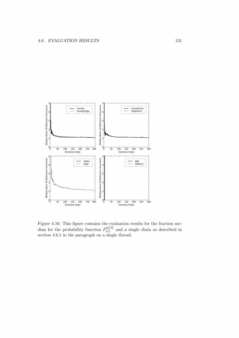
4.6. EVALUATION RESULTS 131
GreedyGreedyEdge
Med
ian
Rati
o O
f Ref
eren
ce S
truc
ture
s
0
1
2
3
4
5
Iteration Steps0 50 100 150 200 250 300
GreedyProjGibbsProj
Med
ian
Rati
o O
f Ref
eren
ce S
truc
ture
s
0
1
2
3
4
5
Iteration Steps0 50 100 150 200 250 300
GibbsEdge
Med
ian
Rati
o O
f Ref
eren
ce S
truc
ture
s
0
1
2
3
4
5
Iteration Steps0 50 100 150 200 250 300
MHMHProj
Med
ian
Rati
o O
f Ref
eren
ce S
truc
ture
s
0
1
2
3
4
5
Iteration Steps0 50 100 150 200 250 300
Figure 4.16: This figure contains the evaluation results for the fraction me-
dian for the probability function Pas5,b
s5
3,5 and a single chain as described insection 4.6.1 in the paragraph on a single thread.
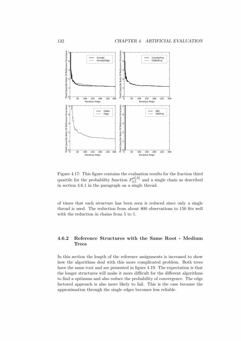
132 CHAPTER 4. ARTIFICIAL EVALUATION
GreedyGreedyEdge
Thir
d Q
uart
ile R
atio
Of R
efer
ence
Str
uctu
res
0
1
2
3
4
5
Iteration Steps0 50 100 150 200 250 300
GreedyProjGibbsProj
Thir
d Q
uart
ile R
atio
Of R
efer
ence
Str
uctu
res
0
1
2
3
4
5
Iteration Steps0 50 100 150 200 250 300
GibbsEdge
Thir
d Q
uart
ile R
atio
Of R
efer
ence
Str
uctu
res
0
1
2
3
4
5
Iteration Steps0 50 100 150 200 250 300
MHMHProj
Thir
d Q
uart
ile R
atio
Of R
efer
ence
Str
uctu
res
0
1
2
3
4
5
Iteration Steps0 50 100 150 200 250 300
Figure 4.17: This figure contains the evaluation results for the fraction third
quartile for the probability function Pas5,b
s5
3,5 and a single chain as describedin section 4.6.1 in the paragraph on a single thread.
of times that each structure has been seen is reduced since only a singlethread is used. The reduction from about 800 observations to 150 fits wellwith the reduction in chains from 5 to 1.
4.6.2 Reference Structures with the Same Root - MediumTrees
In this section the length of the reference assignments is increased to showhow the algorithms deal with this more complicated problem. Both treeshave the same root and are presented in figure 4.19. The expectation is thatthe longer structures will make it more difficult for the different algorithmsto find a optimum and also reduce the probability of convergence. The edgefactored approach is also more likely to fail. This is the case because theapproximation through the single edges becomes less reliable.
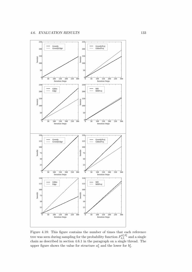
4.6. EVALUATION RESULTS 133
GreedyGreedyEdge
Seen
(a)
0
50
100
150
200
250
Iteration Steps0 50 100 150 200 250 300
GreedyProjGibbsProj
Seen
(a)
0
50
100
150
200
250
Iteration Steps0 50 100 150 200 250 300
GibbsEdge
Seen
(a)
0
50
100
150
200
250
Iteration Steps0 50 100 150 200 250 300
MHMHProj
Seen
(a)
0
50
100
150
200
250
Iteration Steps0 50 100 150 200 250 300
GreedyGreedyEdge
Seen
(b)
0
25
50
75
100
125
150
Iteration Steps0 50 100 150 200 250 300
GreedyProjGibbsProj
Seen
(b)
0
25
50
75
100
125
150
Iteration Steps0 50 100 150 200 250 300
GibbsEdge
Seen
(b)
0
25
50
75
100
125
150
Iteration Steps0 50 100 150 200 250 300
MHMHProj
Seen
(b)
0
25
50
75
100
125
150
Iteration Steps0 50 100 150 200 250 300
Figure 4.18: This figure contains the number of times that each reference
tree was seen during sampling for the probability function Pas5,b
s5
3,5 and a singlechain as described in section 4.6.1 in the paragraph on a single thread. Theupper figure shows the value for structure as5 and the lower for bs5.
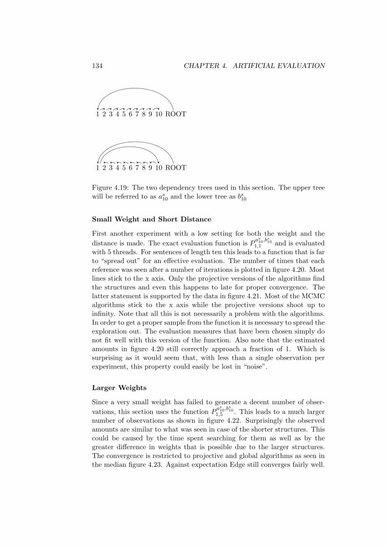
134 CHAPTER 4. ARTIFICIAL EVALUATION
1 2 3 4 5 6 7 8 9 10 ROOT
1 2 3 4 5 6 7 8 9 10 ROOT
Figure 4.19: The two dependency trees used in this section. The upper treewill be referred to as as10 and the lower tree as bs10
Small Weight and Short Distance
First another experiment with a low setting for both the weight and the
distance is made. The exact evaluation function is Pas10,b
s10
1,1 and is evaluatedwith 5 threads. For sentences of length ten this leads to a function that is farto “spread out” for an effective evaluation. The number of times that eachreference was seen after a number of iterations is plotted in figure 4.20. Mostlines stick to the x axis. Only the projective versions of the algorithms findthe structures and even this happens to late for proper convergence. Thelatter statement is supported by the data in figure 4.21. Most of the MCMCalgorithms stick to the x axis while the projective versions shoot up toinfinity. Note that all this is not necessarily a problem with the algorithms.In order to get a proper sample from the function it is necessary to spread theexploration out. The evaluation measures that have been chosen simply donot fit well with this version of the function. Also note that the estimatedamounts in figure 4.20 still correctly approach a fraction of 1. Which issurprising as it would seem that, with less than a single observation perexperiment, this property could easily be lost in “noise”.
Larger Weights
Since a very small weight has failed to generate a decent number of obser-
vations, this section uses the function Pas10,b
s10
1,5 . This leads to a much largernumber of observations as shown in figure 4.22. Surprisingly the observedamounts are similar to what was seen in case of the shorter structures. Thiscould be caused by the time spent searching for them as well as by thegreater difference in weights that is possible due to the larger structures.The convergence is restricted to projective and global algorithms as seen inthe median figure 4.23. Against expectation Edge still converges fairly well.
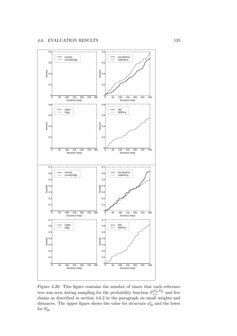
4.6. EVALUATION RESULTS 135
GreedyGreedyEdge
Seen
(a)
0
0.2
0.4
0.6
0.8
Iteration Steps0 50 100 150 200 250 300
GreedyProjGibbsProj
Seen
(a)
0
0.2
0.4
0.6
0.8
Iteration Steps0 50 100 150 200 250 300
GibbsEdge
Seen
(a)
0
0.2
0.4
0.6
0.8
Iteration Steps0 50 100 150 200 250 300
MHMHProj
Seen
(a)
0
0.2
0.4
0.6
0.8
Iteration Steps0 50 100 150 200 250 300
GreedyGreedyEdge
Seen
(b)
0
0.1
0.2
0.3
0.4
0.5
0.6
0.7
Iteration Steps0 50 100 150 200 250 300
GreedyProjGibbsProj
Seen
(b)
0
0.1
0.2
0.3
0.4
0.5
0.6
0.7
Iteration Steps0 50 100 150 200 250 300
GibbsEdge
Seen
(b)
0
0.1
0.2
0.3
0.4
0.5
0.6
0.7
Iteration Steps0 50 100 150 200 250 300
MHMHProj
Seen
(b)
0
0.1
0.2
0.3
0.4
0.5
0.6
0.7
Iteration Steps0 50 100 150 200 250 300
Figure 4.20: This figure contains the number of times that each reference
tree was seen during sampling for the probability function Pas10,b
s10
1,1 and fivechains as described in section 4.6.2 in the paragraph on small weights anddistances. The upper figure shows the value for structure as10 and the lowerfor bs10.
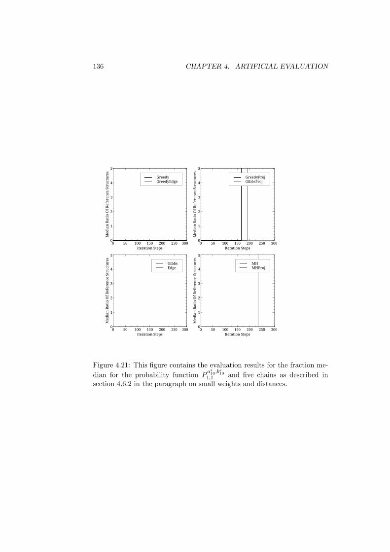
136 CHAPTER 4. ARTIFICIAL EVALUATION
GreedyGreedyEdge
Med
ian
Rati
o O
f Ref
eren
ce S
truc
ture
s
0
1
2
3
4
5
Iteration Steps0 50 100 150 200 250 300
GreedyProjGibbsProj
Med
ian
Rati
o O
f Ref
eren
ce S
truc
ture
s
0
1
2
3
4
5
Iteration Steps0 50 100 150 200 250 300
GibbsEdge
Med
ian
Rati
o O
f Ref
eren
ce S
truc
ture
s
0
1
2
3
4
5
Iteration Steps0 50 100 150 200 250 300
MHMHProj
Med
ian
Rati
o O
f Ref
eren
ce S
truc
ture
s
0
1
2
3
4
5
Iteration Steps0 50 100 150 200 250 300
Figure 4.21: This figure contains the evaluation results for the fraction me-
dian for the probability function Pas10,b
s10
1,1 and five chains as described insection 4.6.2 in the paragraph on small weights and distances.
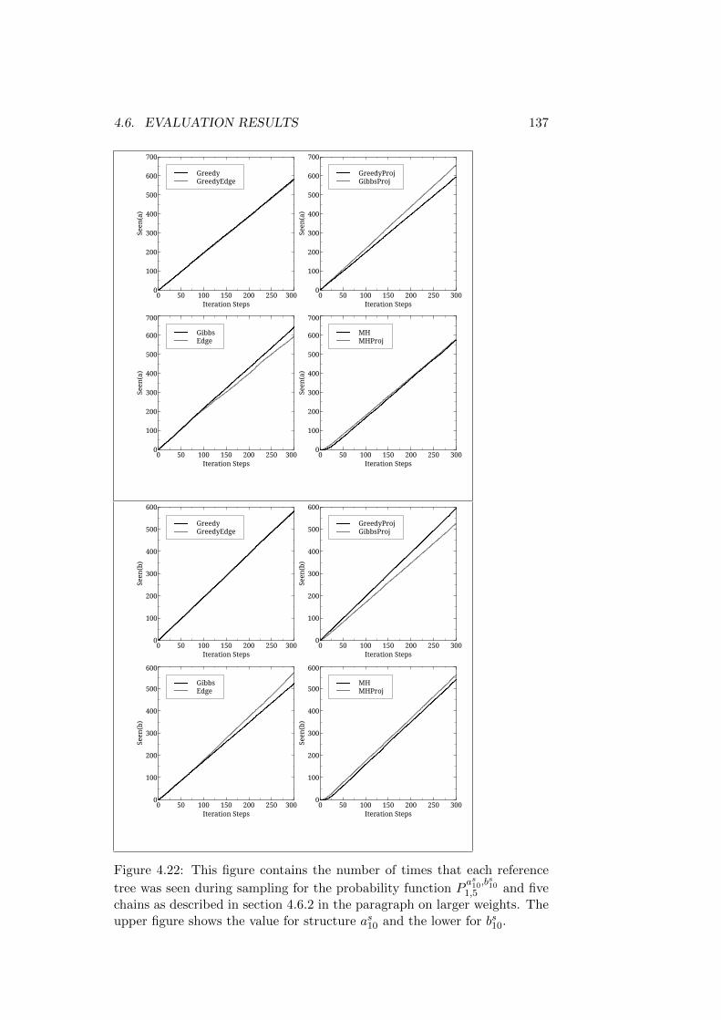
4.6. EVALUATION RESULTS 137
GreedyGreedyEdge
Seen
(a)
0
100
200
300
400
500
600
700
Iteration Steps0 50 100 150 200 250 300
GreedyProjGibbsProj
Seen
(a)
0
100
200
300
400
500
600
700
Iteration Steps0 50 100 150 200 250 300
GibbsEdge
Seen
(a)
0
100
200
300
400
500
600
700
Iteration Steps0 50 100 150 200 250 300
MHMHProj
Seen
(a)
0
100
200
300
400
500
600
700
Iteration Steps0 50 100 150 200 250 300
GreedyGreedyEdge
Seen
(b)
0
100
200
300
400
500
600
Iteration Steps0 50 100 150 200 250 300
GreedyProjGibbsProj
Seen
(b)
0
100
200
300
400
500
600
Iteration Steps0 50 100 150 200 250 300
GibbsEdge
Seen
(b)
0
100
200
300
400
500
600
Iteration Steps0 50 100 150 200 250 300
MHMHProj
Seen
(b)
0
100
200
300
400
500
600
Iteration Steps0 50 100 150 200 250 300
Figure 4.22: This figure contains the number of times that each reference
tree was seen during sampling for the probability function Pas10,b
s10
1,5 and fivechains as described in section 4.6.2 in the paragraph on larger weights. Theupper figure shows the value for structure as10 and the lower for bs10.

138 CHAPTER 4. ARTIFICIAL EVALUATION
GreedyGreedyEdge
Med
ian
Rati
o O
f Ref
eren
ce S
truc
ture
s
0
1
2
3
4
5
Iteration Steps0 50 100 150 200 250 300
GreedyProjGibbsProj
Med
ian
Rati
o O
f Ref
eren
ce S
truc
ture
s
0
1
2
3
4
5
Iteration Steps0 50 100 150 200 250 300
GibbsEdge
Med
ian
Rati
o O
f Ref
eren
ce S
truc
ture
s
0
1
2
3
4
5
Iteration Steps0 50 100 150 200 250 300
MHMHProj
Med
ian
Rati
o O
f Ref
eren
ce S
truc
ture
s
0
1
2
3
4
5
Iteration Steps0 50 100 150 200 250 300
Figure 4.23: This figure contains the evaluation results for the fraction me-
dian for the probability function Pas10,b
s10
1,5 and five chains as described insection 4.6.2 in the paragraph on larger weights.
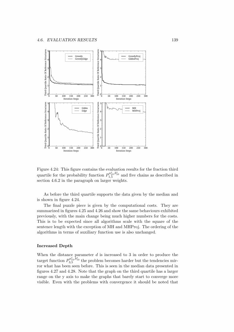
4.6. EVALUATION RESULTS 139
GreedyGreedyEdge
Thir
d Q
uart
ile R
atio
Of R
efer
ence
Str
uctu
res
0
1
2
3
4
5
Iteration Steps0 50 100 150 200 250 300
GreedyProjGibbsProj
Thir
d Q
uart
ile R
atio
Of R
efer
ence
Str
uctu
res
0
1
2
3
4
5
Iteration Steps0 50 100 150 200 250 300
GibbsEdge
Thir
d Q
uart
ile R
atio
Of R
efer
ence
Str
uctu
res
0
1
2
3
4
5
Iteration Steps0 50 100 150 200 250 300
MHMHProj
Thir
d Q
uart
ile R
atio
Of R
efer
ence
Str
uctu
res
0
1
2
3
4
5
Iteration Steps0 50 100 150 200 250 300
Figure 4.24: This figure contains the evaluation results for the fraction third
quartile for the probability function Pas10,b
s10
1,5 and five chains as described insection 4.6.2 in the paragraph on larger weights.
As before the third quartile supports the data given by the median andis shown in figure 4.24.
The final puzzle piece is given by the computational costs. They aresummarized in figures 4.25 and 4.26 and show the same behaviours exhibitedpreviously, with the main change being much higher numbers for the costs.This is to be expected since all algorithms scale with the square of thesentence length with the exception of MH and MHProj. The ordering of thealgorithms in terms of auxiliary function use is also unchanged.
Increased Depth
When the distance parameter d is increased to 3 in order to produce the
target function Pas10,b
s10
3,5 the problem becomes harder but the tendencies mir-ror what has been seen before. This is seen in the median data presented infigures 4.27 and 4.28. Note that the graph on the third quartile has a largerrange on the y axis to make the graphs that barely start to converge morevisible. Even with the problems with convergence it should be noted that
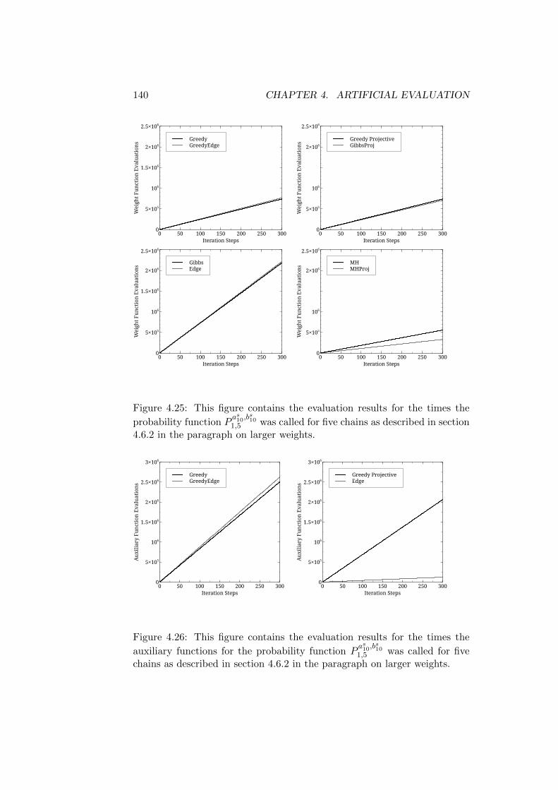
140 CHAPTER 4. ARTIFICIAL EVALUATION
GreedyGreedyEdge
Wei
ght F
unct
ion
Eval
uati
ons
0
5×10⁵
106
1.5×10⁶
2×10⁶
2.5×10⁶
Iteration Steps0 50 100 150 200 250 300
Greedy ProjectiveGibbsProj
Wei
ght F
unct
ion
Eval
uati
ons
0
5×10⁵
106
2×10⁶
2.5×10⁶
Iteration Steps0 50 100 150 200 250 300
GibbsEdge
Wei
ght F
unct
ion
Eval
uati
ons
0
5×10⁵
106
1.5×10⁶
2×10⁶
2.5×10⁶
Iteration Steps0 50 100 150 200 250 300
MHMHProj
Wei
ght F
unct
ion
Eval
uati
ons
0
5×10⁵
106
2×10⁶
2.5×10⁶
Iteration Steps0 50 100 150 200 250 300
Figure 4.25: This figure contains the evaluation results for the times the
probability function Pas10,b
s10
1,5 was called for five chains as described in section4.6.2 in the paragraph on larger weights.
GreedyGreedyEdge
Aux
iliar
y Fu
ncti
on E
valu
atio
ns
0
5×10⁵
106
1.5×10⁶
2×10⁶
2.5×10⁶
3×10⁶
Iteration Steps0 50 100 150 200 250 300
Greedy ProjectiveEdge
Aux
iliar
y Fu
ncti
on E
valu
atio
ns
0
5×10⁵
106
1.5×10⁶
2×10⁶
2.5×10⁶
3×10⁶
Iteration Steps0 50 100 150 200 250 300
Figure 4.26: This figure contains the evaluation results for the times the
auxiliary functions for the probability function Pas10,b
s10
1,5 was called for fivechains as described in section 4.6.2 in the paragraph on larger weights.
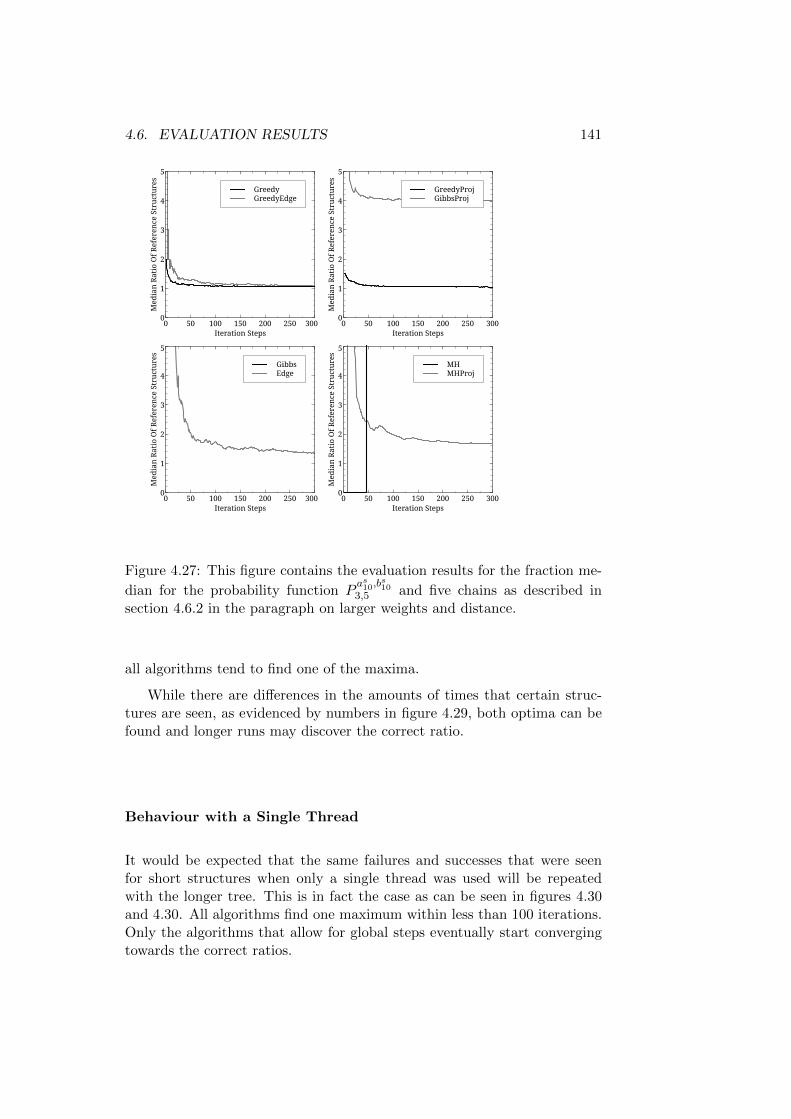
4.6. EVALUATION RESULTS 141
GreedyGreedyEdge
Med
ian
Rati
o O
f Ref
eren
ce S
truc
ture
s
0
1
2
3
4
5
Iteration Steps0 50 100 150 200 250 300
GreedyProjGibbsProj
Med
ian
Rati
o O
f Ref
eren
ce S
truc
ture
s0
1
2
3
4
5
Iteration Steps0 50 100 150 200 250 300
GibbsEdge
Med
ian
Rati
o O
f Ref
eren
ce S
truc
ture
s
0
1
2
3
4
5
Iteration Steps0 50 100 150 200 250 300
MHMHProj
Med
ian
Rati
o O
f Ref
eren
ce S
truc
ture
s
0
1
2
3
4
5
Iteration Steps0 50 100 150 200 250 300
Figure 4.27: This figure contains the evaluation results for the fraction me-
dian for the probability function Pas10,b
s10
3,5 and five chains as described insection 4.6.2 in the paragraph on larger weights and distance.
all algorithms tend to find one of the maxima.
While there are differences in the amounts of times that certain struc-tures are seen, as evidenced by numbers in figure 4.29, both optima can befound and longer runs may discover the correct ratio.
Behaviour with a Single Thread
It would be expected that the same failures and successes that were seenfor short structures when only a single thread was used will be repeatedwith the longer tree. This is in fact the case as can be seen in figures 4.30and 4.30. All algorithms find one maximum within less than 100 iterations.Only the algorithms that allow for global steps eventually start convergingtowards the correct ratios.
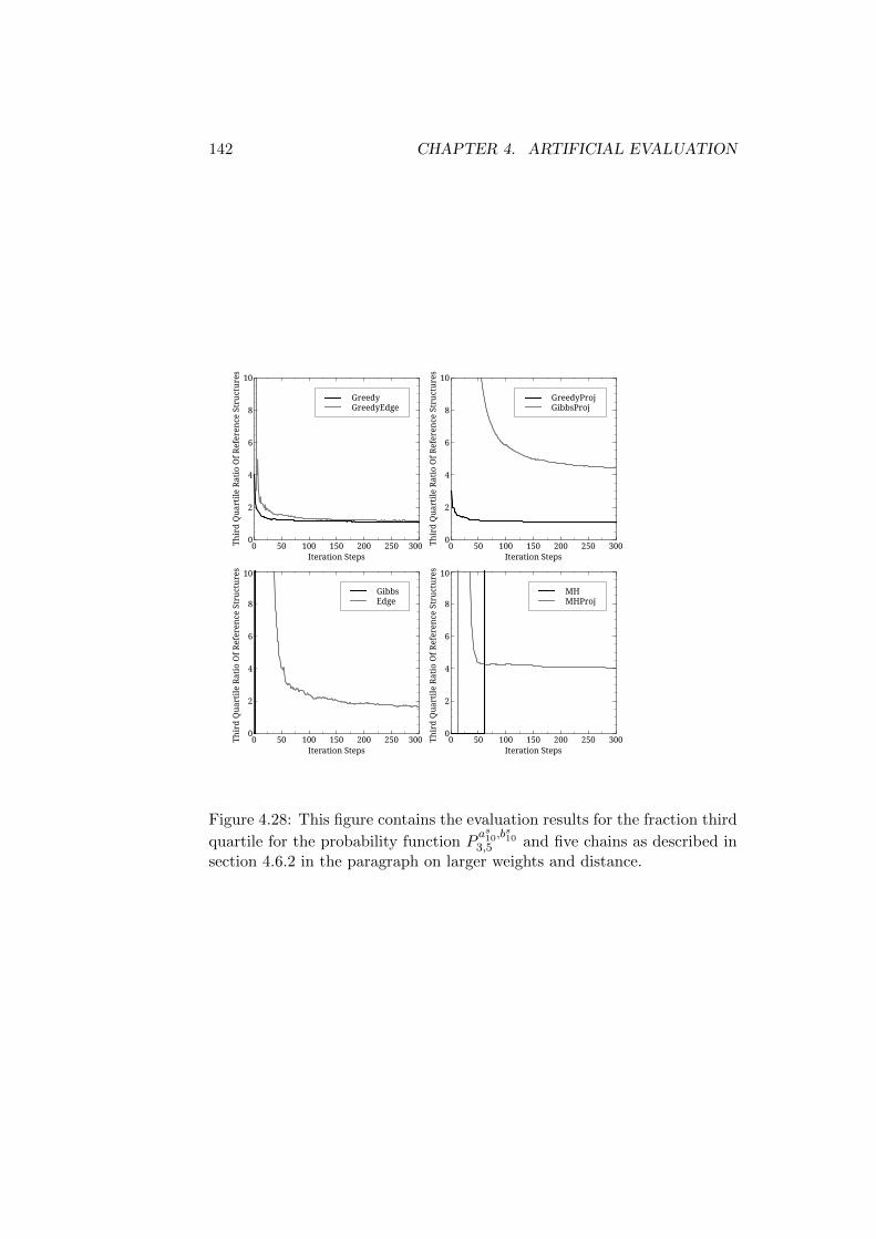
142 CHAPTER 4. ARTIFICIAL EVALUATION
GreedyGreedyEdge
Thir
d Q
uart
ile R
atio
Of R
efer
ence
Str
uctu
res
0
2
4
6
8
10
Iteration Steps0 50 100 150 200 250 300
GreedyProjGibbsProj
Thir
d Q
uart
ile R
atio
Of R
efer
ence
Str
uctu
res
0
2
4
6
8
10
Iteration Steps0 50 100 150 200 250 300
GibbsEdge
Thir
d Q
uart
ile R
atio
Of R
efer
ence
Str
uctu
res
0
2
4
6
8
10
Iteration Steps0 50 100 150 200 250 300
MHMHProj
Thir
d Q
uart
ile R
atio
Of R
efer
ence
Str
uctu
res
0
2
4
6
8
10
Iteration Steps0 50 100 150 200 250 300
Figure 4.28: This figure contains the evaluation results for the fraction third
quartile for the probability function Pas10,b
s10
3,5 and five chains as described insection 4.6.2 in the paragraph on larger weights and distance.
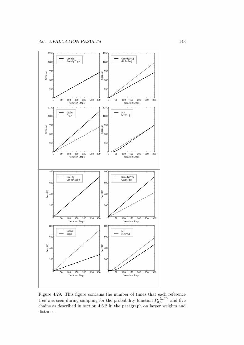
4.6. EVALUATION RESULTS 143
GreedyGreedyEdge
Seen
(a)
0
250
500
750
1000
1250
Iteration Steps0 50 100 150 200 250 300
GreedyProjGibbsProj
Seen
(a)
0
250
500
750
1000
1250
Iteration Steps0 50 100 150 200 250 300
GibbsEdge
Seen
(a)
0
250
500
750
1000
1250
Iteration Steps0 50 100 150 200 250 300
MHMHProj
Seen
(a)
0
250
500
750
1000
1250
Iteration Steps0 50 100 150 200 250 300
GreedyGreedyEdge
Seen
(b)
0
200
400
600
800
Iteration Steps0 50 100 150 200 250 300
GreedyProjGibbsProj
Seen
(b)
0
200
400
600
800
Iteration Steps0 50 100 150 200 250 300
GibbsEdge
Seen
(b)
0
200
400
600
800
Iteration Steps0 50 100 150 200 250 300
MHMHProj
Seen
(b)
0
200
400
600
800
Iteration Steps0 50 100 150 200 250 300
Figure 4.29: This figure contains the number of times that each reference
tree was seen during sampling for the probability function Pas10,b
s10
3,5 and fivechains as described in section 4.6.2 in the paragraph on larger weights anddistance.
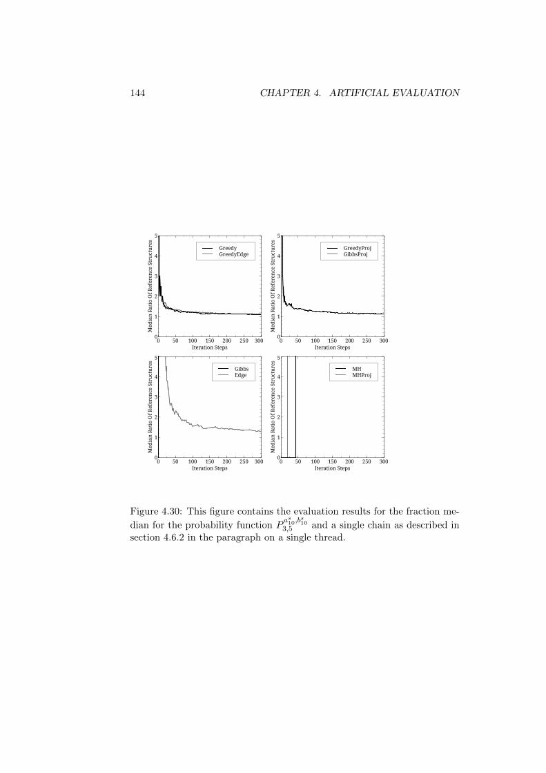
144 CHAPTER 4. ARTIFICIAL EVALUATION
GreedyGreedyEdge
Med
ian
Rati
o O
f Ref
eren
ce S
truc
ture
s
0
1
2
3
4
5
Iteration Steps0 50 100 150 200 250 300
GreedyProjGibbsProj
Med
ian
Rati
o O
f Ref
eren
ce S
truc
ture
s
0
1
2
3
4
5
Iteration Steps0 50 100 150 200 250 300
GibbsEdge
Med
ian
Rati
o O
f Ref
eren
ce S
truc
ture
s
0
1
2
3
4
5
Iteration Steps0 50 100 150 200 250 300
MHMHProj
Med
ian
Rati
o O
f Ref
eren
ce S
truc
ture
s
0
1
2
3
4
5
Iteration Steps0 50 100 150 200 250 300
Figure 4.30: This figure contains the evaluation results for the fraction me-
dian for the probability function Pas10,b
s10
3,5 and a single chain as described insection 4.6.2 in the paragraph on a single thread.
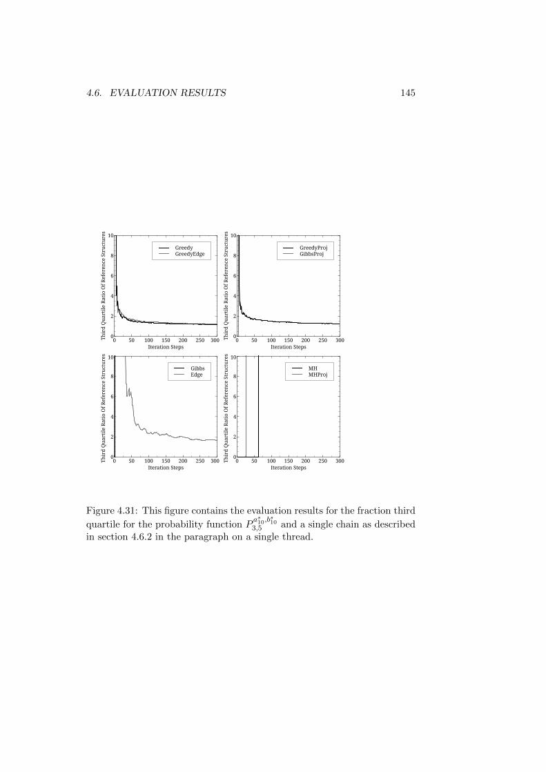
4.6. EVALUATION RESULTS 145
GreedyGreedyEdge
Thir
d Q
uart
ile R
atio
Of R
efer
ence
Str
uctu
res
0
2
4
6
8
10
Iteration Steps0 50 100 150 200 250 300
GreedyProjGibbsProj
Thir
d Q
uart
ile R
atio
Of R
efer
ence
Str
uctu
res
0
2
4
6
8
10
Iteration Steps0 50 100 150 200 250 300
GibbsEdge
Thir
d Q
uart
ile R
atio
Of R
efer
ence
Str
uctu
res
0
2
4
6
8
10
Iteration Steps0 50 100 150 200 250 300
MHMHProj
Thir
d Q
uart
ile R
atio
Of R
efer
ence
Str
uctu
res
0
2
4
6
8
10
Iteration Steps0 50 100 150 200 250 300
Figure 4.31: This figure contains the evaluation results for the fraction third
quartile for the probability function Pas10,b
s10
3,5 and a single chain as describedin section 4.6.2 in the paragraph on a single thread.
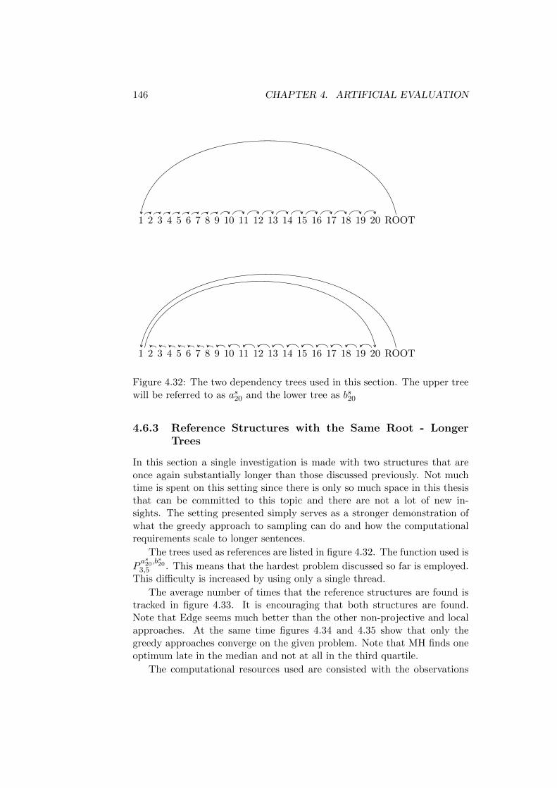
146 CHAPTER 4. ARTIFICIAL EVALUATION
1 2 3 4 5 6 7 8 9 10 11 12 13 14 15 16 17 18 19 20 ROOT
1 2 3 4 5 6 7 8 9 10 11 12 13 14 15 16 17 18 19 20 ROOT
Figure 4.32: The two dependency trees used in this section. The upper treewill be referred to as as20 and the lower tree as bs20
4.6.3 Reference Structures with the Same Root - LongerTrees
In this section a single investigation is made with two structures that areonce again substantially longer than those discussed previously. Not muchtime is spent on this setting since there is only so much space in this thesisthat can be committed to this topic and there are not a lot of new in-sights. The setting presented simply serves as a stronger demonstration ofwhat the greedy approach to sampling can do and how the computationalrequirements scale to longer sentences.
The trees used as references are listed in figure 4.32. The function used is
Pas20,b
s20
3,5 . This means that the hardest problem discussed so far is employed.This difficulty is increased by using only a single thread.
The average number of times that the reference structures are found istracked in figure 4.33. It is encouraging that both structures are found.Note that Edge seems much better than the other non-projective and localapproaches. At the same time figures 4.34 and 4.35 show that only thegreedy approaches converge on the given problem. Note that MH finds oneoptimum late in the median and not at all in the third quartile.
The computational resources used are consisted with the observations
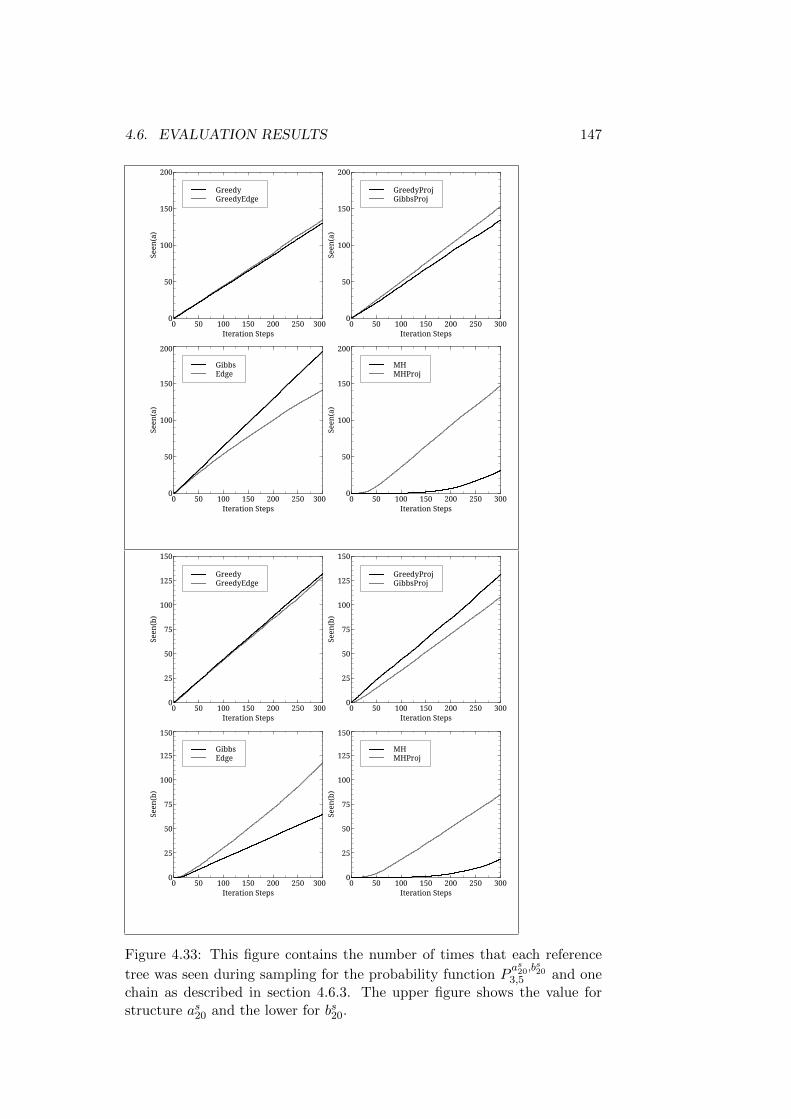
4.6. EVALUATION RESULTS 147
GreedyGreedyEdge
Seen
(a)
0
50
100
150
200
Iteration Steps0 50 100 150 200 250 300
GreedyProjGibbsProj
Seen
(a)
0
50
100
150
200
Iteration Steps0 50 100 150 200 250 300
GibbsEdge
Seen
(a)
0
50
100
150
200
Iteration Steps0 50 100 150 200 250 300
MHMHProj
Seen
(a)
0
50
100
150
200
Iteration Steps0 50 100 150 200 250 300
GreedyGreedyEdge
Seen
(b)
0
25
50
75
100
125
150
Iteration Steps0 50 100 150 200 250 300
GreedyProjGibbsProj
Seen
(b)
0
25
50
75
100
125
150
Iteration Steps0 50 100 150 200 250 300
GibbsEdge
Seen
(b)
0
25
50
75
100
125
150
Iteration Steps0 50 100 150 200 250 300
MHMHProj
Seen
(b)
0
25
50
75
100
125
150
Iteration Steps0 50 100 150 200 250 300
Figure 4.33: This figure contains the number of times that each reference
tree was seen during sampling for the probability function Pas20,b
s20
3,5 and onechain as described in section 4.6.3. The upper figure shows the value forstructure as20 and the lower for bs20.

148 CHAPTER 4. ARTIFICIAL EVALUATION
GreedyGreedyEdge
Med
ian
Rati
o O
f Ref
eren
ce S
truc
ture
s
0
1
2
3
4
5
Iteration Steps0 50 100 150 200 250 300
GreedyProjGibbsProj
Med
ian
Rati
o O
f Ref
eren
ce S
truc
ture
s
0
1
2
3
4
5
Iteration Steps0 50 100 150 200 250 300
GibbsEdge
Med
ian
Rati
o O
f Ref
eren
ce S
truc
ture
s
0
1
2
3
4
5
Iteration Steps0 50 100 150 200 250 300
MHMHProj
Med
ian
Rati
o O
f Ref
eren
ce S
truc
ture
s
0
1
2
3
4
5
Iteration Steps0 50 100 150 200 250 300
Figure 4.34: This figure contains the evaluation results for the fraction me-
dian for the probability function Pas20,b
s20
3,5 and one chain as described in sec-tion 4.6.3.

4.6. EVALUATION RESULTS 149
GreedyGreedyEdge
Thir
d Q
uart
ile R
atio
Of R
efer
ence
Str
uctu
res
0
2
4
6
8
10
Iteration Steps0 50 100 150 200 250 300
GreedyProjGibbsProj
Thir
d Q
uart
ile R
atio
Of R
efer
ence
Str
uctu
res
0
2
4
6
8
10
Iteration Steps0 50 100 150 200 250 300
GibbsEdge
Thir
d Q
uart
ile R
atio
Of R
efer
ence
Str
uctu
res
0
2
4
6
8
10
Iteration Steps0 50 100 150 200 250 300
MHMHProj
Thir
d Q
uart
ile R
atio
Of R
efer
ence
Str
uctu
res
0
2
4
6
8
10
Iteration Steps0 50 100 150 200 250 300
Figure 4.35: This figure contains the evaluation results for the fraction third
quartile for the probability function Pas20,b
s20
3,5 and one chain as described insection 4.6.3.
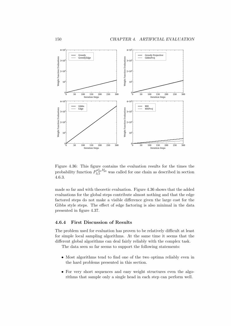
150 CHAPTER 4. ARTIFICIAL EVALUATION
GreedyGreedyEdge
Wei
ght F
unct
ion
Eval
uati
ons
0
106
2×10⁶
3×10⁶
4×10⁶
Iteration Steps0 50 100 150 200 250 300
Greedy ProjectiveGibbsProj
Wei
ght F
unct
ion
Eval
uati
ons
0
106
2×10⁶
3×10⁶
4×10⁶
Iteration Steps0 50 100 150 200 250 300
GibbsEdge
Wei
ght F
unct
ion
Eval
uati
ons
0
106
2×10⁶
3×10⁶
4×10⁶
Iteration Steps0 50 100 150 200 250 300
MHMHProj
Wei
ght F
unct
ion
Eval
uati
ons
0
106
2×10⁶
3×10⁶
4×10⁶
Iteration Steps0 50 100 150 200 250 300
Figure 4.36: This figure contains the evaluation results for the times the
probability function Pas20,b
s20
3,5 was called for one chain as described in section4.6.3.
made so far and with theoretic evaluation. Figure 4.36 shows that the addedevaluations for the global steps contribute almost nothing and that the edgefactored steps do not make a visible difference given the large cost for theGibbs style steps. The effect of edge factoring is also minimal in the datapresented in figure 4.37.
4.6.4 First Discussion of Results
The problem used for evaluation has proven to be relatively difficult at leastfor simple local sampling algorithms. At the same time it seems that thedifferent global algorithms can deal fairly reliably with the complex task.
The data seen so far seems to support the following statements:
• Most algorithms tend to find one of the two optima reliably even inthe hard problems presented in this section.
• For very short sequences and easy weight structures even the algo-rithms that sample only a single head in each step can perform well.
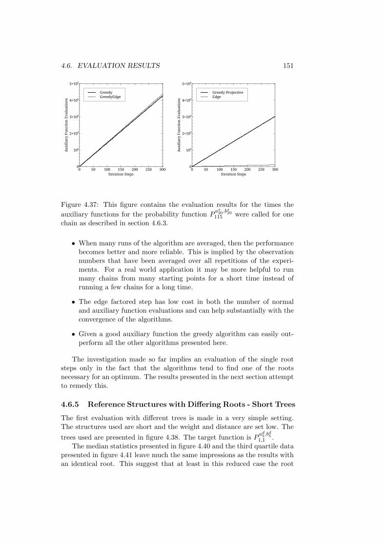
4.6. EVALUATION RESULTS 151
GreedyGreedyEdge
Aux
iliar
y Fu
ncti
on E
valu
atio
ns
0
106
2×10⁶
3×10⁶
4×10⁶
5×10⁶
Iteration Steps0 50 100 150 200 250 300
Greedy ProjectiveEdge
Aux
iliar
y Fu
ncti
on E
valu
atio
ns
0
106
2×10⁶
3×10⁶
4×10⁶
5×10⁶
Iteration Steps0 50 100 150 200 250 300
Figure 4.37: This figure contains the evaluation results for the times the
auxiliary functions for the probability function Pas20,b
s20
115 were called for onechain as described in section 4.6.3.
• When many runs of the algorithm are averaged, then the performancebecomes better and more reliable. This is implied by the observationnumbers that have been averaged over all repetitions of the experi-ments. For a real world application it may be more helpful to runmany chains from many starting points for a short time instead ofrunning a few chains for a long time.
• The edge factored step has low cost in both the number of normaland auxiliary function evaluations and can help substantially with theconvergence of the algorithms.
• Given a good auxiliary function the greedy algorithm can easily out-perform all the other algorithms presented here.
The investigation made so far implies an evaluation of the single rootsteps only in the fact that the algorithms tend to find one of the rootsnecessary for an optimum. The results presented in the next section attemptto remedy this.
4.6.5 Reference Structures with Differing Roots - Short Trees
The first evaluation with different trees is made in a very simple setting.The structures used are short and the weight and distance are set low. The
trees used are presented in figure 4.38. The target function is Pad5,b
d5
1,1 .The median statistics presented in figure 4.40 and the third quartile data
presented in figure 4.41 leave much the same impressions as the results withan identical root. This suggest that at least in this reduced case the root
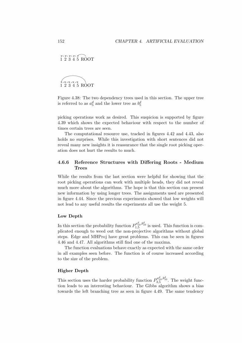
152 CHAPTER 4. ARTIFICIAL EVALUATION
1 2 3 4 5 ROOT
1 2 3 4 5 ROOT
Figure 4.38: The two dependency trees used in this section. The upper treeis referred to as ad5 and the lower tree as bd5
picking operations work as desired. This suspicion is supported by figure4.39 which shows the expected behaviour with respect to the number oftimes certain trees are seen.
The computational resource use, tracked in figures 4.42 and 4.43, alsoholds no surprises. While this investigation with short sentences did notreveal many new insights it is reassurance that the single root picking oper-ation does not hurt the results to much.
4.6.6 Reference Structures with Differing Roots - MediumTrees
While the results from the last section were helpful for showing that theroot picking operations can work with multiple heads, they did not revealmuch more about the algorithms. The hope is that this section can presentnew information by using longer trees. The assignments used are presentedin figure 4.44. Since the previous experiments showed that low weights willnot lead to any useful results the experiments all use the weight 5.
Low Depth
In this section the probability function Pad10,b
d10
1,5 is used. This function is com-plicated enough to weed out the non-projective algorithms without globalsteps. Edge and MHProj have great problems. This can be seen in figures4.46 and 4.47. All algorithms still find one of the maxima.
The function evaluations behave exactly as expected with the same orderin all examples seen before. The function is of course increased accordingto the size of the problem.
Higher Depth
This section uses the harder probability function Pad10,b
d10
3,5 . The weight func-tion leads to an interesting behaviour. The Gibbs algorithm shows a biastowards the left branching tree as seen in figure 4.49. The same tendency
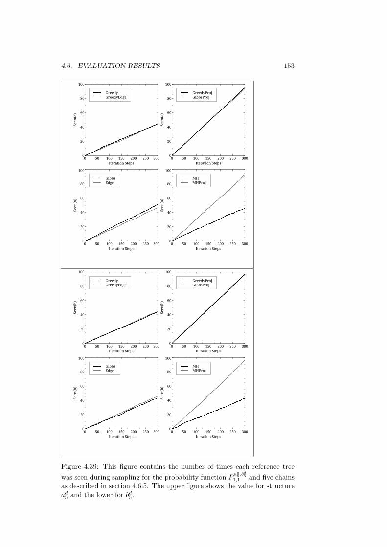
4.6. EVALUATION RESULTS 153
GreedyGreedyEdge
Seen
(a)
0
20
40
60
80
100
Iteration Steps0 50 100 150 200 250 300
GreedyProjGibbsProj
Seen
(a)
0
20
40
60
80
100
Iteration Steps0 50 100 150 200 250 300
GibbsEdge
Seen
(a)
0
20
40
60
80
100
Iteration Steps0 50 100 150 200 250 300
MHMHProj
Seen
(a)
0
20
40
60
80
100
Iteration Steps0 50 100 150 200 250 300
GreedyGreedyEdge
Seen
(b)
0
20
40
60
80
100
Iteration Steps0 50 100 150 200 250 300
GreedyProjGibbsProj
Seen
(b)
0
20
40
60
80
100
Iteration Steps0 50 100 150 200 250 300
GibbsEdge
Seen
(b)
0
20
40
60
80
100
Iteration Steps0 50 100 150 200 250 300
MHMHProj
Seen
(b)
0
20
40
60
80
100
Iteration Steps0 50 100 150 200 250 300
Figure 4.39: This figure contains the number of times each reference tree
was seen during sampling for the probability function Pad5,b
d5
1,1 and five chainsas described in section 4.6.5. The upper figure shows the value for structuread5 and the lower for bd5.
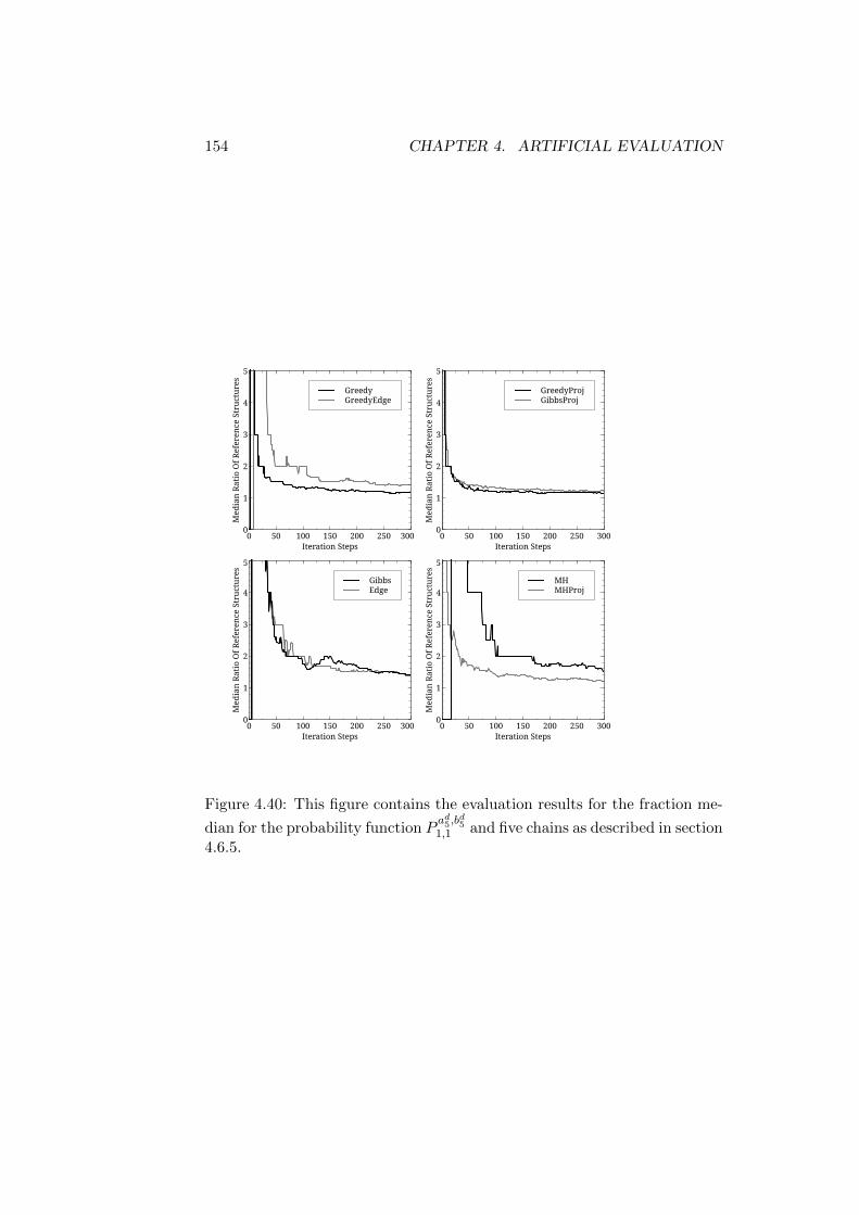
154 CHAPTER 4. ARTIFICIAL EVALUATION
GreedyGreedyEdge
Med
ian
Rati
o O
f Ref
eren
ce S
truc
ture
s
0
1
2
3
4
5
Iteration Steps0 50 100 150 200 250 300
GreedyProjGibbsProj
Med
ian
Rati
o O
f Ref
eren
ce S
truc
ture
s
0
1
2
3
4
5
Iteration Steps0 50 100 150 200 250 300
GibbsEdge
Med
ian
Rati
o O
f Ref
eren
ce S
truc
ture
s
0
1
2
3
4
5
Iteration Steps0 50 100 150 200 250 300
MHMHProj
Med
ian
Rati
o O
f Ref
eren
ce S
truc
ture
s
0
1
2
3
4
5
Iteration Steps0 50 100 150 200 250 300
Figure 4.40: This figure contains the evaluation results for the fraction me-
dian for the probability function Pad5,b
d5
1,1 and five chains as described in section4.6.5.
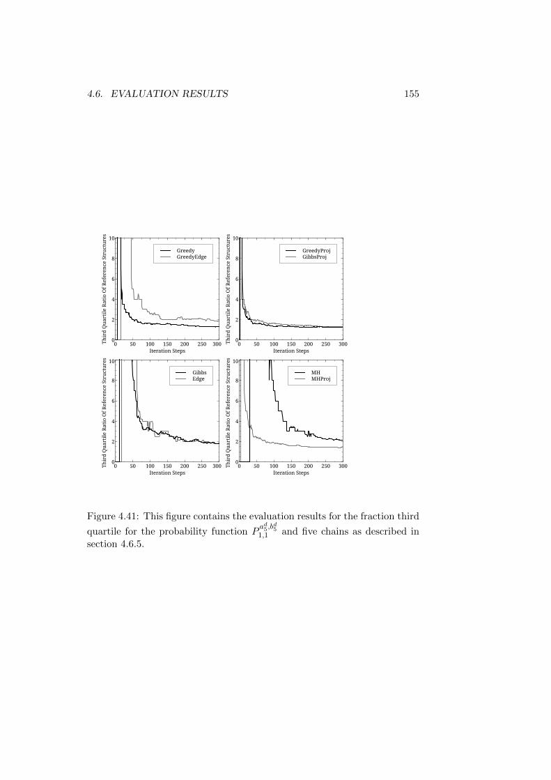
4.6. EVALUATION RESULTS 155
GreedyGreedyEdge
Thir
d Q
uart
ile R
atio
Of R
efer
ence
Str
uctu
res
0
2
4
6
8
10
Iteration Steps0 50 100 150 200 250 300
GreedyProjGibbsProj
Thir
d Q
uart
ile R
atio
Of R
efer
ence
Str
uctu
res
0
2
4
6
8
10
Iteration Steps0 50 100 150 200 250 300
GibbsEdge
Thir
d Q
uart
ile R
atio
Of R
efer
ence
Str
uctu
res
0
2
4
6
8
10
Iteration Steps0 50 100 150 200 250 300
MHMHProj
Thir
d Q
uart
ile R
atio
Of R
efer
ence
Str
uctu
res
0
2
4
6
8
10
Iteration Steps0 50 100 150 200 250 300
Figure 4.41: This figure contains the evaluation results for the fraction third
quartile for the probability function Pad5,b
d5
1,1 and five chains as described insection 4.6.5.

156 CHAPTER 4. ARTIFICIAL EVALUATION
GreedyGreedyEdge
Wei
ght F
unct
ion
Eval
uati
ons
0
5×10⁴
105
1.5×10⁵
2×10⁵
2.5×10⁵
3×10⁵
Iteration Steps0 50 100 150 200 250 300
Greedy ProjectiveGibbsProj
Wei
ght F
unct
ion
Eval
uati
ons
0
5×10⁴
105
2×10⁵
3×10⁵
Iteration Steps0 50 100 150 200 250 300
GibbsEdge
Wei
ght F
unct
ion
Eval
uati
ons
0
5×10⁴
105
1.5×10⁵
2×10⁵
2.5×10⁵
3×10⁵
Iteration Steps0 50 100 150 200 250 300
MHMHProj
Wei
ght F
unct
ion
Eval
uati
ons
0
5×10⁴
105
2×10⁵
3×10⁵
Iteration Steps0 50 100 150 200 250 300
Figure 4.42: This figure contains the evaluation results for the times the
probability function Pad5,b
d5
1,1 was called for five chains as described in section4.6.5.
GreedyGreedyEdge
Aux
iliar
y Fu
ncti
on E
valu
atio
ns
0
5×10⁴
105
1.5×10⁵
2×10⁵
2.5×10⁵
3×10⁵
3.5×10⁵
Iteration Steps0 50 100 150 200 250 300
Greedy ProjectiveEdge
Aux
iliar
y Fu
ncti
on E
valu
atio
ns
0
5×10⁴
105
1.5×10⁵
2×10⁵
2.5×10⁵
3×10⁵
3.5×10⁵
Iteration Steps0 50 100 150 200 250 300
Figure 4.43: This figure contains the evaluation results for the times the
auxiliary functions for the probability function Pad5,b
d5
1,1 was called for fivechains as described in section 4.6.5.
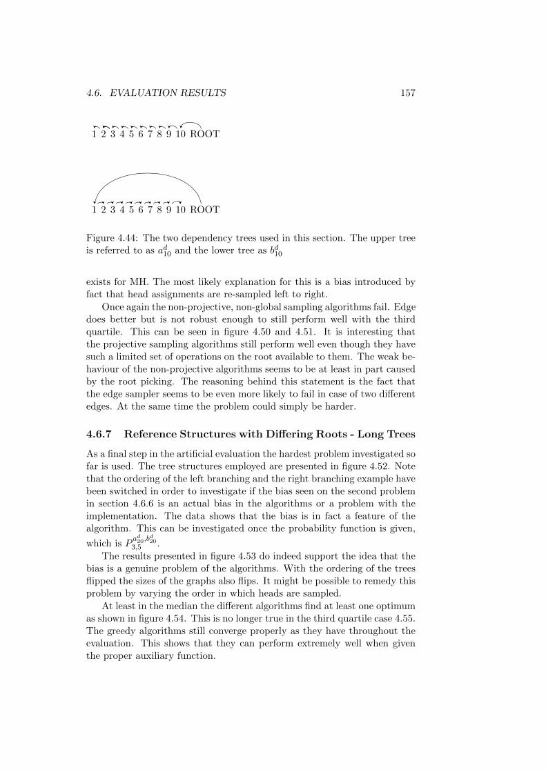
4.6. EVALUATION RESULTS 157
1 2 3 4 5 6 7 8 9 10 ROOT
1 2 3 4 5 6 7 8 9 10 ROOT
Figure 4.44: The two dependency trees used in this section. The upper treeis referred to as ad10 and the lower tree as bd10
exists for MH. The most likely explanation for this is a bias introduced byfact that head assignments are re-sampled left to right.
Once again the non-projective, non-global sampling algorithms fail. Edgedoes better but is not robust enough to still perform well with the thirdquartile. This can be seen in figure 4.50 and 4.51. It is interesting thatthe projective sampling algorithms still perform well even though they havesuch a limited set of operations on the root available to them. The weak be-haviour of the non-projective algorithms seems to be at least in part causedby the root picking. The reasoning behind this statement is the fact thatthe edge sampler seems to be even more likely to fail in case of two differentedges. At the same time the problem could simply be harder.
4.6.7 Reference Structures with Differing Roots - Long Trees
As a final step in the artificial evaluation the hardest problem investigated sofar is used. The tree structures employed are presented in figure 4.52. Notethat the ordering of the left branching and the right branching example havebeen switched in order to investigate if the bias seen on the second problemin section 4.6.6 is an actual bias in the algorithms or a problem with theimplementation. The data shows that the bias is in fact a feature of thealgorithm. This can be investigated once the probability function is given,
which is Pad20,b
d20
3,5 .
The results presented in figure 4.53 do indeed support the idea that thebias is a genuine problem of the algorithms. With the ordering of the treesflipped the sizes of the graphs also flips. It might be possible to remedy thisproblem by varying the order in which heads are sampled.
At least in the median the different algorithms find at least one optimumas shown in figure 4.54. This is no longer true in the third quartile case 4.55.The greedy algorithms still converge properly as they have throughout theevaluation. This shows that they can perform extremely well when giventhe proper auxiliary function.
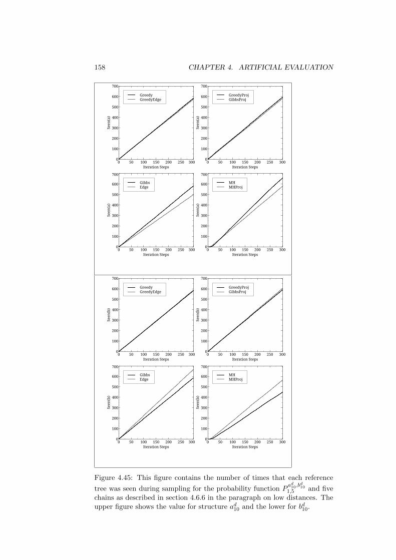
158 CHAPTER 4. ARTIFICIAL EVALUATION
GreedyGreedyEdge
Seen
(a)
0
100
200
300
400
500
600
700
Iteration Steps0 50 100 150 200 250 300
GreedyProjGibbsProj
Seen
(a)
0
100
200
300
400
500
600
700
Iteration Steps0 50 100 150 200 250 300
GibbsEdge
Seen
(a)
0
100
200
300
400
500
600
700
Iteration Steps0 50 100 150 200 250 300
MHMHProj
Seen
(a)
0
100
200
300
400
500
600
700
Iteration Steps0 50 100 150 200 250 300
GreedyGreedyEdge
Seen
(b)
0
100
200
300
400
500
600
700
Iteration Steps0 50 100 150 200 250 300
GreedyProjGibbsProj
Seen
(b)
0
100
200
300
400
500
600
700
Iteration Steps0 50 100 150 200 250 300
GibbsEdge
Seen
(b)
0
100
200
300
400
500
600
700
Iteration Steps0 50 100 150 200 250 300
MHMHProj
Seen
(b)
0
100
200
300
400
500
600
700
Iteration Steps0 50 100 150 200 250 300
Figure 4.45: This figure contains the number of times that each reference
tree was seen during sampling for the probability function Pad10,b
d10
1,5 and fivechains as described in section 4.6.6 in the paragraph on low distances. Theupper figure shows the value for structure ad10 and the lower for bd10.
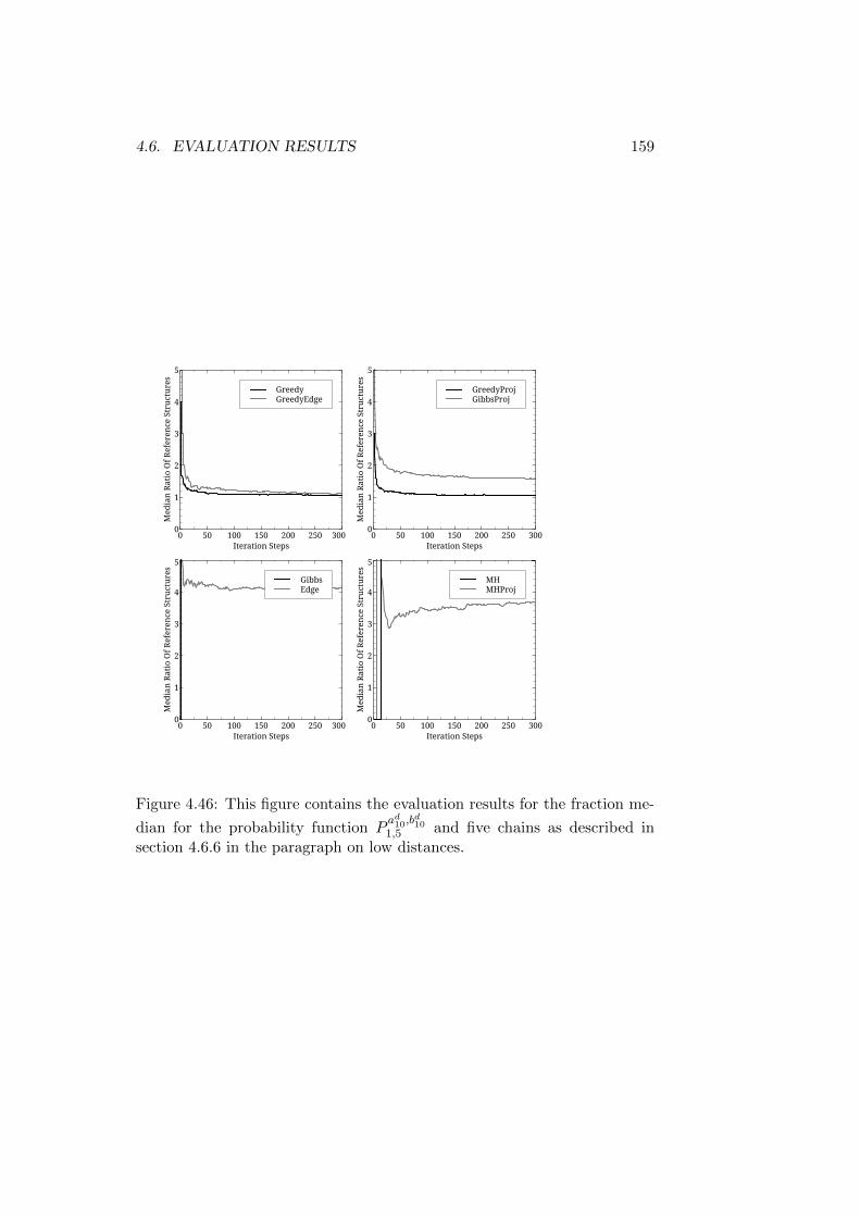
4.6. EVALUATION RESULTS 159
GreedyGreedyEdge
Med
ian
Rati
o O
f Ref
eren
ce S
truc
ture
s
0
1
2
3
4
5
Iteration Steps0 50 100 150 200 250 300
GreedyProjGibbsProj
Med
ian
Rati
o O
f Ref
eren
ce S
truc
ture
s
0
1
2
3
4
5
Iteration Steps0 50 100 150 200 250 300
GibbsEdge
Med
ian
Rati
o O
f Ref
eren
ce S
truc
ture
s
0
1
2
3
4
5
Iteration Steps0 50 100 150 200 250 300
MHMHProj
Med
ian
Rati
o O
f Ref
eren
ce S
truc
ture
s
0
1
2
3
4
5
Iteration Steps0 50 100 150 200 250 300
Figure 4.46: This figure contains the evaluation results for the fraction me-
dian for the probability function Pad10,b
d10
1,5 and five chains as described insection 4.6.6 in the paragraph on low distances.
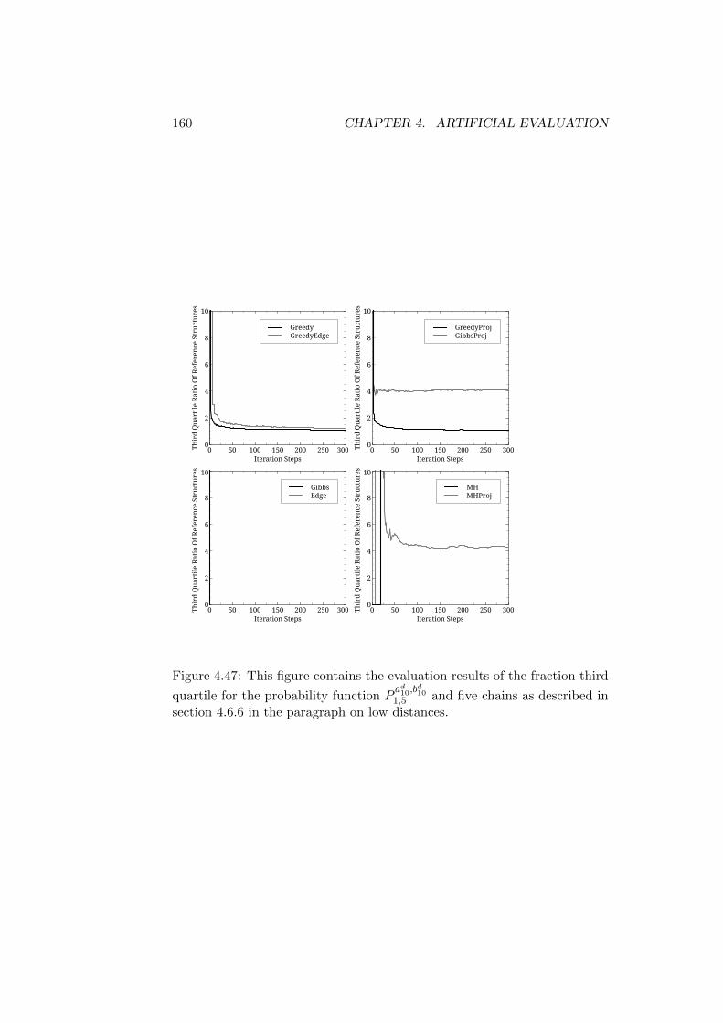
160 CHAPTER 4. ARTIFICIAL EVALUATION
GreedyGreedyEdge
Thir
d Q
uart
ile R
atio
Of R
efer
ence
Str
uctu
res
0
2
4
6
8
10
Iteration Steps0 50 100 150 200 250 300
GreedyProjGibbsProj
Thir
d Q
uart
ile R
atio
Of R
efer
ence
Str
uctu
res
0
2
4
6
8
10
Iteration Steps0 50 100 150 200 250 300
GibbsEdge
Thir
d Q
uart
ile R
atio
Of R
efer
ence
Str
uctu
res
0
2
4
6
8
10
Iteration Steps0 50 100 150 200 250 300
MHMHProj
Thir
d Q
uart
ile R
atio
Of R
efer
ence
Str
uctu
res
0
2
4
6
8
10
Iteration Steps0 50 100 150 200 250 300
Figure 4.47: This figure contains the evaluation results of the fraction third
quartile for the probability function Pad10,b
d10
1,5 and five chains as described insection 4.6.6 in the paragraph on low distances.
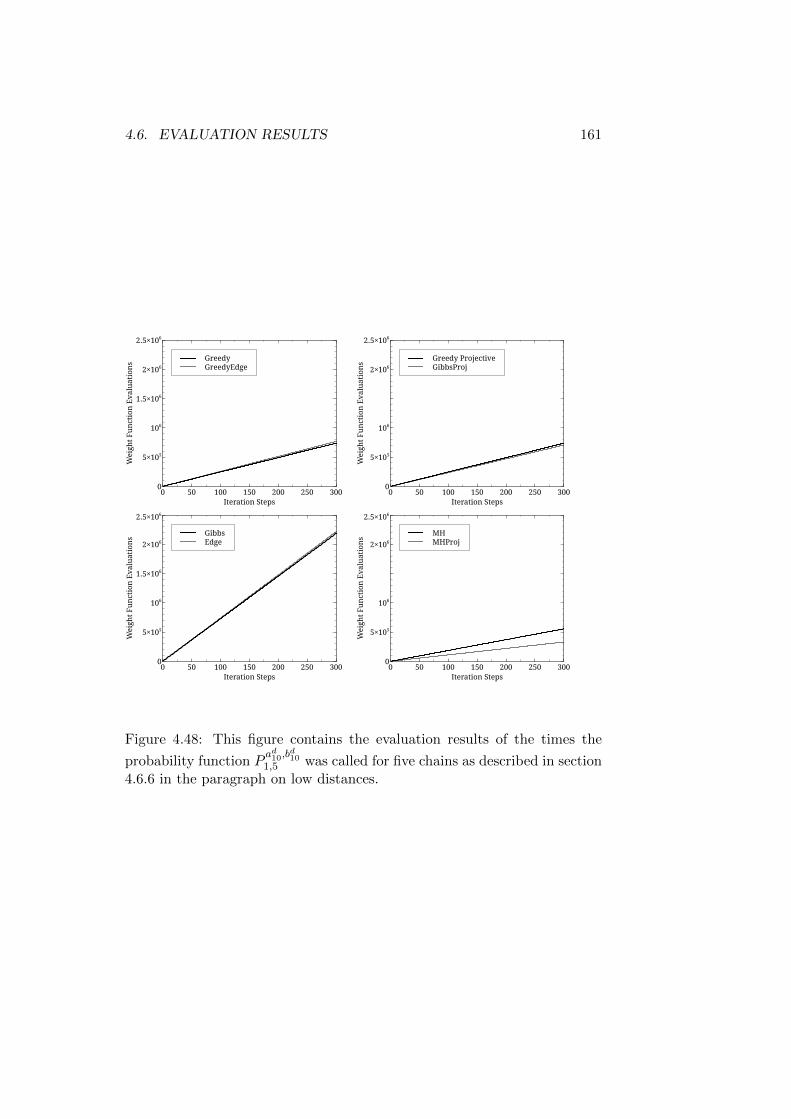
4.6. EVALUATION RESULTS 161
GreedyGreedyEdge
Wei
ght F
unct
ion
Eval
uati
ons
0
5×10⁵
106
1.5×10⁶
2×10⁶
2.5×10⁶
Iteration Steps0 50 100 150 200 250 300
Greedy ProjectiveGibbsProj
Wei
ght F
unct
ion
Eval
uati
ons
0
5×10⁵
106
2×10⁶
2.5×10⁶
Iteration Steps0 50 100 150 200 250 300
GibbsEdge
Wei
ght F
unct
ion
Eval
uati
ons
0
5×10⁵
106
1.5×10⁶
2×10⁶
2.5×10⁶
Iteration Steps0 50 100 150 200 250 300
MHMHProj
Wei
ght F
unct
ion
Eval
uati
ons
0
5×10⁵
106
2×10⁶
2.5×10⁶
Iteration Steps0 50 100 150 200 250 300
Figure 4.48: This figure contains the evaluation results of the times the
probability function Pad10,b
d10
1,5 was called for five chains as described in section4.6.6 in the paragraph on low distances.
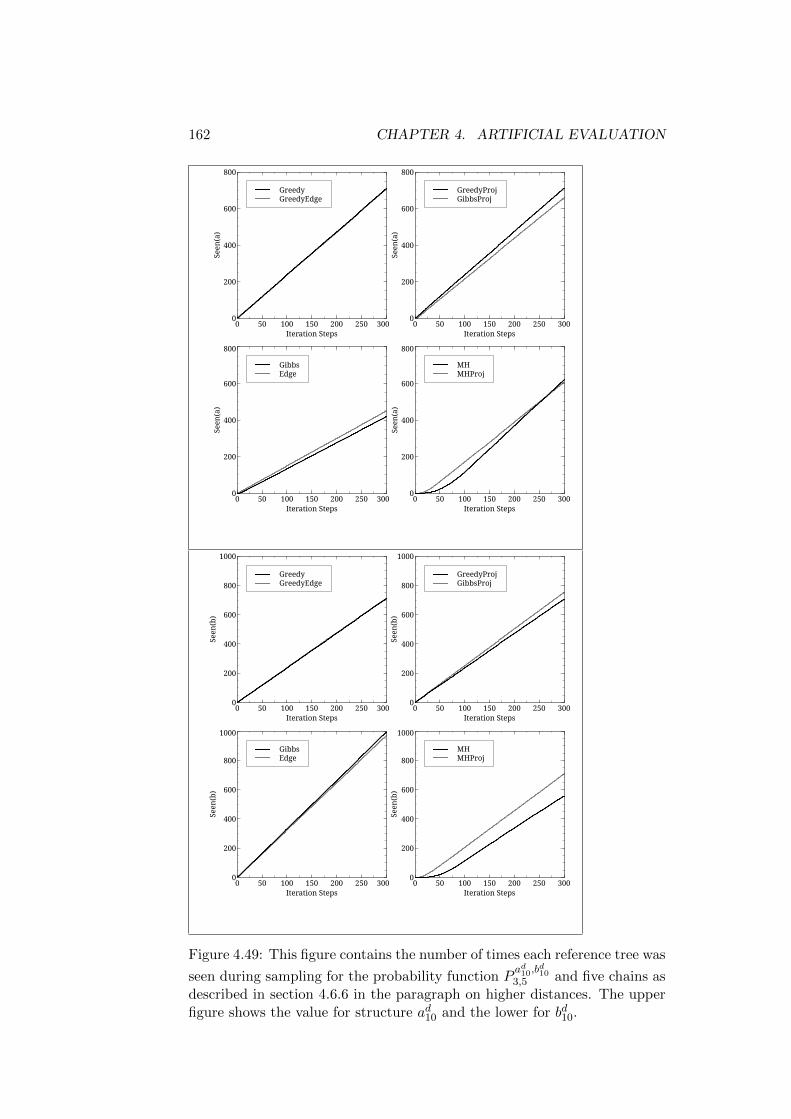
162 CHAPTER 4. ARTIFICIAL EVALUATION
GreedyGreedyEdge
Seen
(a)
0
200
400
600
800
Iteration Steps0 50 100 150 200 250 300
GreedyProjGibbsProj
Seen
(a)
0
200
400
600
800
Iteration Steps0 50 100 150 200 250 300
GibbsEdge
Seen
(a)
0
200
400
600
800
Iteration Steps0 50 100 150 200 250 300
MHMHProj
Seen
(a)
0
200
400
600
800
Iteration Steps0 50 100 150 200 250 300
GreedyGreedyEdge
Seen
(b)
0
200
400
600
800
1000
Iteration Steps0 50 100 150 200 250 300
GreedyProjGibbsProj
Seen
(b)
0
200
400
600
800
1000
Iteration Steps0 50 100 150 200 250 300
GibbsEdge
Seen
(b)
0
200
400
600
800
1000
Iteration Steps0 50 100 150 200 250 300
MHMHProj
Seen
(b)
0
200
400
600
800
1000
Iteration Steps0 50 100 150 200 250 300
Figure 4.49: This figure contains the number of times each reference tree was
seen during sampling for the probability function Pad10,b
d10
3,5 and five chains asdescribed in section 4.6.6 in the paragraph on higher distances. The upperfigure shows the value for structure ad10 and the lower for bd10.

4.6. EVALUATION RESULTS 163
GreedyGreedyEdge
Med
ian
Rati
o O
f Ref
eren
ce S
truc
ture
s
0
1
2
3
4
5
Iteration Steps0 50 100 150 200 250 300
GreedyProjGibbsProj
Med
ian
Rati
o O
f Ref
eren
ce S
truc
ture
s
0
1
2
3
4
5
Iteration Steps0 50 100 150 200 250 300
GibbsEdge
Med
ian
Rati
o O
f Ref
eren
ce S
truc
ture
s
0
1
2
3
4
5
Iteration Steps0 50 100 150 200 250 300
MHMHProj
Med
ian
Rati
o O
f Ref
eren
ce S
truc
ture
s
0
1
2
3
4
5
Iteration Steps0 50 100 150 200 250 300
Figure 4.50: This figure contains the evaluation results of the fraction me-
dian for the probability function Pad10,b
d10
3,5 and five chains as described insection 4.6.6 in the paragraph on higher distances.
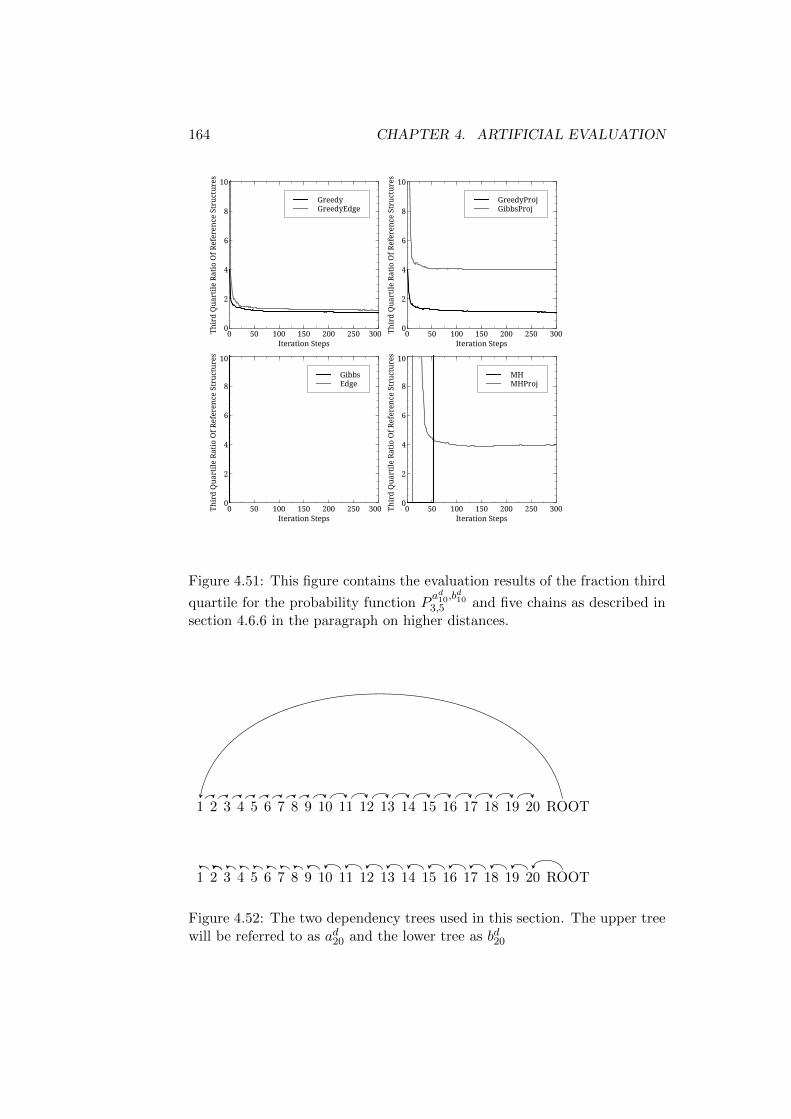
164 CHAPTER 4. ARTIFICIAL EVALUATION
GreedyGreedyEdge
Thir
d Q
uart
ile R
atio
Of R
efer
ence
Str
uctu
res
0
2
4
6
8
10
Iteration Steps0 50 100 150 200 250 300
GreedyProjGibbsProj
Thir
d Q
uart
ile R
atio
Of R
efer
ence
Str
uctu
res
0
2
4
6
8
10
Iteration Steps0 50 100 150 200 250 300
GibbsEdge
Thir
d Q
uart
ile R
atio
Of R
efer
ence
Str
uctu
res
0
2
4
6
8
10
Iteration Steps0 50 100 150 200 250 300
MHMHProj
Thir
d Q
uart
ile R
atio
Of R
efer
ence
Str
uctu
res
0
2
4
6
8
10
Iteration Steps0 50 100 150 200 250 300
Figure 4.51: This figure contains the evaluation results of the fraction third
quartile for the probability function Pad10,b
d10
3,5 and five chains as described insection 4.6.6 in the paragraph on higher distances.
1 2 3 4 5 6 7 8 9 10 11 12 13 14 15 16 17 18 19 20 ROOT
1 2 3 4 5 6 7 8 9 10 11 12 13 14 15 16 17 18 19 20 ROOT
Figure 4.52: The two dependency trees used in this section. The upper treewill be referred to as ad20 and the lower tree as bd20
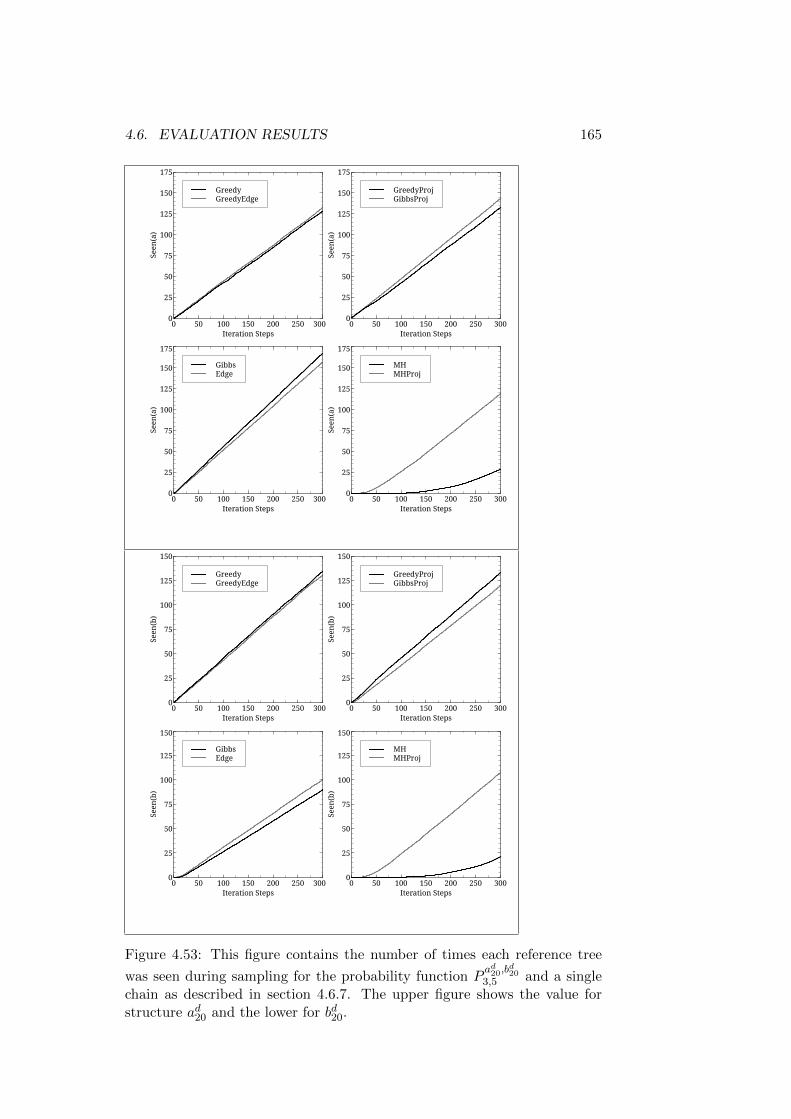
4.6. EVALUATION RESULTS 165
GreedyGreedyEdge
Seen
(a)
0
25
50
75
100
125
150
175
Iteration Steps0 50 100 150 200 250 300
GreedyProjGibbsProj
Seen
(a)
0
25
50
75
100
125
150
175
Iteration Steps0 50 100 150 200 250 300
GibbsEdge
Seen
(a)
0
25
50
75
100
125
150
175
Iteration Steps0 50 100 150 200 250 300
MHMHProj
Seen
(a)
0
25
50
75
100
125
150
175
Iteration Steps0 50 100 150 200 250 300
GreedyGreedyEdge
Seen
(b)
0
25
50
75
100
125
150
Iteration Steps0 50 100 150 200 250 300
GreedyProjGibbsProj
Seen
(b)
0
25
50
75
100
125
150
Iteration Steps0 50 100 150 200 250 300
GibbsEdge
Seen
(b)
0
25
50
75
100
125
150
Iteration Steps0 50 100 150 200 250 300
MHMHProj
Seen
(b)
0
25
50
75
100
125
150
Iteration Steps0 50 100 150 200 250 300
Figure 4.53: This figure contains the number of times each reference tree
was seen during sampling for the probability function Pad20,b
d20
3,5 and a singlechain as described in section 4.6.7. The upper figure shows the value forstructure ad20 and the lower for bd20.
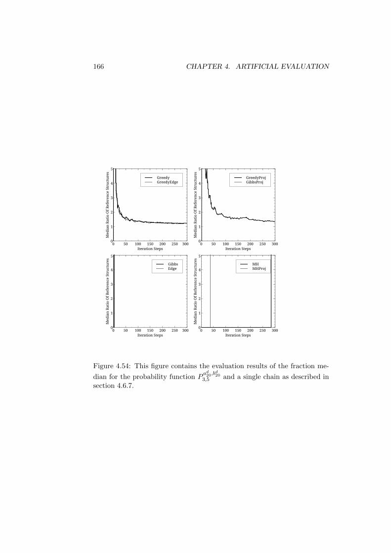
166 CHAPTER 4. ARTIFICIAL EVALUATION
GreedyGreedyEdge
Med
ian
Rati
o O
f Ref
eren
ce S
truc
ture
s
0
1
2
3
4
5
Iteration Steps0 50 100 150 200 250 300
GreedyProjGibbsProj
Med
ian
Rati
o O
f Ref
eren
ce S
truc
ture
s
0
1
2
3
4
5
Iteration Steps0 50 100 150 200 250 300
GibbsEdge
Med
ian
Rati
o O
f Ref
eren
ce S
truc
ture
s
0
1
2
3
4
5
Iteration Steps0 50 100 150 200 250 300
MHMHProj
Med
ian
Rati
o O
f Ref
eren
ce S
truc
ture
s
0
1
2
3
4
5
Iteration Steps0 50 100 150 200 250 300
Figure 4.54: This figure contains the evaluation results of the fraction me-
dian for the probability function Pad20,b
d20
3,5 and a single chain as described insection 4.6.7.
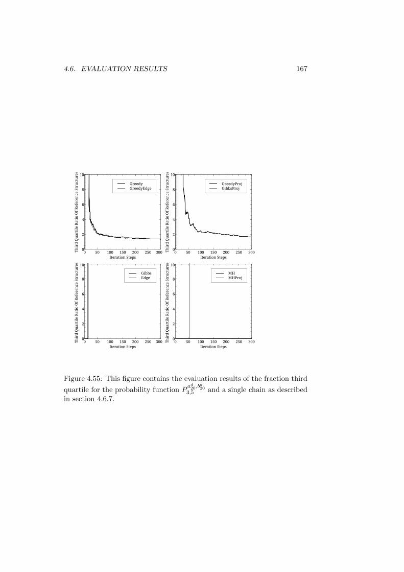
4.6. EVALUATION RESULTS 167
GreedyGreedyEdge
Thir
d Q
uart
ile R
atio
Of R
efer
ence
Str
uctu
res
0
2
4
6
8
10
Iteration Steps0 50 100 150 200 250 300
GreedyProjGibbsProj
Thir
d Q
uart
ile R
atio
Of R
efer
ence
Str
uctu
res
0
2
4
6
8
10
Iteration Steps0 50 100 150 200 250 300
GibbsEdge
Thir
d Q
uart
ile R
atio
Of R
efer
ence
Str
uctu
res
0
2
4
6
8
10
Iteration Steps0 50 100 150 200 250 300
MHMHProj
Thir
d Q
uart
ile R
atio
Of R
efer
ence
Str
uctu
res
0
2
4
6
8
10
Iteration Steps0 50 100 150 200 250 300
Figure 4.55: This figure contains the evaluation results of the fraction third
quartile for the probability function Pad20,b
d20
3,5 and a single chain as describedin section 4.6.7.
168 CHAPTER 4. ARTIFICIAL EVALUATION
4.7 Conclusions and Future Research
The evaluation results presented in this chapter can be used to support anumber of claims:
1. The algorithms based on greedy proposals can perform extremely wellwhen given a good approximation of the probability function.
2. Global MCMC steps are useful in dealing with multiple optima in theprobability function.
3. Depending on the auxiliary function greedy sampling may be muchmore expensive than edge factored sampling but this additional costcan result in much better performance.
4. The MCMC schemes have no problem finding at least one optimum.This is easily explained by the fact that, save for MH and MHProj,they all include some version of the systematic Gibbs style search. Ifthe target function has only a single optimum, then a Gibbs basedsampler might be a good choice because they found the optima withina few sampling steps.
5. It seems generally beneficent to average out an extended number ofparallel chains. This enables each chain to find one optimum similarto random restarting in optimization problems.
6. The simple scheme based on uniform proposals can be competitivewith the Gibbs based approach at a much smaller cost.
7. The restriction of movements that is implied by a restriction to projec-tive structures is more than made up for by the reduction in possiblestructures to explore and the projective samplers tend to perform bet-ter and cheaper than their non-projective counterpart.
Most of these statements are not surprising except maybe for the lastthree points. In chapter 5 another task is presented that can be used tofurther investigate the claims made. It should be noted that the results pre-sented here represent only a fraction of the data that was actually generatedfor this thesis. Reviewing all the results would expand this thesis beyondany reasonable bounds. As mentioned before the author of this thesis canbe contacted for all the remaining experimental results and the code thatwas used will be made publicly available.
An interesting observation is the apparent bias the samplers have withrespect to certain structures. As mentioned before, this could be causedby the order in which heads are sampled and it might be the case that thesampling results could be improved by changing this order. The greedy

4.7. CONCLUSIONS AND FUTURE RESEARCH 169
sampling step actually does this, but it is not clear whether this contributesto its very good performance. investigating this is left for further study. Alsoleft for further study is the use of edge factored samplers that are based onthe Matrix Tree Theorem. The current sampler uses the edge factoring tocreate a complete graph given the root but a sampler based computing actualweights could be used to assign the root node on this basis. This could helpthe edge factored sampler in the scenario where two different roots are used.Overall the performance of Edge was still better than expected.
It would be interesting the to study the probability function that wasused in this chapter with a slight difference in weight between the two struc-tures and see if this difference would be reflected in the behaviour of thechains, but this would also further expand a chapter that is already veryfull with graphs and might strain the patience of the reader. It would bevery easy to implement the idea in a follow-up study. Such a study couldalso experiment with switching the different root samplers. The Gibbs ap-proach to root sampling made the algorithms that used it rather costly. Asthe uniform approach to root sampling performs almost as well, it might bepossible to save a large number of function evaluations

170 CHAPTER 4. ARTIFICIAL EVALUATION
Chapter 5
Evaluation on anUnsupervised DependencyParsing Task
In this chapter a second evaluation task is presented. This problem is basedon the unsupervised or weakly supervised learning of dependency trees fora corpus tagged with gold standard Part-Of-Speech (POS) tags [45]. Theobjective of this task is to predict dependency trees for natural languagesentences without ever using any dependency trees as input. In supervisedlearning for dependency parsing the prediction of dependency trees is usuallybased on selecting a model that somehow “does well” on a set of trainingsentences which have been hand annotated [59]. The resulting model isthen used to generate trees for new sentences. Unsupervised dependencyparsing removes the need for any sentences which are already annotatedfor dependency. This is of great interest for Natural Language Processingsince there is a high time cost for hand annotating sentences1[90]. Thereare a number of tasks that can profit from using dependency parses asinput such as semantic processing [24, 16, 42] or language modelling [43].If unsupervised dependency parsing were able to perform in a way that iscompetitive with supervised dependency parsing, then it would be easy toextend tools based on dependency trees to under-resourced languages andnew domains. For POS tagging there are already attempts to make use ofunsupervised approaches in languages that lack resources [25]. Even withina language it will often be necessary to adapt to new domains such as theTwitter data that has become available in the last years [47, 66]. Employinga model derived from one domain in another is a non-trivial task [96] eventhough it is currently performing better than unsupervised learning.
Current evaluations of unsupervised learning for tasks such as depen-
1Usually thousands of sentences are needed for good performance of the supervisedapproaches
171
172 CHAPTER 5. UNSUPERVISED PARSING EVALUATION
dency parsing and POS tagging [45] show that it performs worse than adapt-ing models from one language to another [108] or semi-supervised learning[96, 71] and it will be seen in future research which approach will become theprevalent choice. In this thesis the unsupervised dependency parsing taskis chosen since it requires a difficult learning problem that can be solved bysampling.
The concept of weakly supervised dependency parsing is an extensionof unsupervised parsing that attempts to improve the performance of unsu-pervised algorithms with small amount of information that can usually beobtained easily. One example would be the writing of small sets of rules thatcan help in selecting parse trees [80]. Another would be the use of HTMLannotation to guide selections on edge directions [106].
Unsupervised dependency parsing has an extended history in NaturalLanguage Processing as can be seen from the short review given in [57] andreceived more attention in recent years [45]. In section 5.1 a short reviewof existing approaches will be given. Then there will be a presentation ofthe alignment model by Brody [12]. This is the model used for evaluationof the dependency samplers from this thesis. The reason why this model isused is that is is very natural to demand that there is only a single root ina sentence when this model is used. Sampling has been used for inferencewith this model and the approach has been formulated in a way that is veryamendable to sampling. It does not perform at state-of-the-art levels, butachieving great performance is not the main goal of this section. Instead it isinvestigated how well the different sampling algorithms do on the inferencetask. This evaluation is somewhat problematic since it is not possible tocompute any interesting expectations for the model without making use ofsome approximation algorithm, otherwise there would be no reason to evenuse the MCMC algorithms. Instead of tracking convergence towards someknown statistic, evaluation is based on the weight of the annotation foundaccording to the model. In order to evaluate the convergence and the qualityof the resulting parses an existing dataset will be used which is presented insection 5.5. Then evaluation results are then given in the following sections.
5.1 State of the Art in Unsupervised DependencyParsing
The dominant model for unsupervised dependency parsing in recent yearshas been the Dependency Model with Valence (DMV) that was originallyintroduced by Klein and Manning [57]. The idea for the model is based onan observation by the authors that existing dependency models tended toonly make use of the frequency with which words or tags tended to occurtogether. They suggested that it would be important to also model thefertility of a word. This means that any model should also have some concept
5.1. STATE OF THE ART 173
of how many children any word is likely to have. The model attempts todescribe the way a dependency tree is generated by breaking it up into theindividual decisions to generate each child word one by one i.e. decidingto generate another child in one direction and then deciding which childnodes to actually generate. The probabilities for each of these decisions isonly based on POS tags and makes no use of the actual words. There areextensions to the model that make use of words, but even these extensionsonly use the most frequent ones [52].
This seemingly simple model has gained a lot of attention in the lit-erature. Since unsupervised learning usually makes it necessary to guidea learning algorithm towards results of a certain type a lot of the papersthat used this model combine it with some learning paradigm that the au-thors wish to investigate. Among the approaches that have been used isBayesian learning based on Variational Inference [22]. There the authorsattempted to guide learning by connecting the values of the different pa-rameters that need to be estimated. Another technique tested was usingmore global restrictions on the structures that were induced in a frameworkcalled posterior regularization [41]. A similar approach by Tu [110] that alsomade used of the DMV was one of the best performing participators in the2012 Pascal Challenge on Grammar induction [45]. It has been shown thatViterbi Training, i.e. the use of only the best performing tree assignmentsin an iterative training approach like Expectation Maximization, can leadto good results in combination with the DMV [105, 100]. It is especiallyinteresting that the Viterbi approach seems to be relatively robust with re-spect to initialization. This is important since most algorithms based on theDMV are very dependent on the initialization they used. If a technique forinference with this model attempts to reduce the influence of initialization,then the performance can easily deteriorate [93]. This is also the main rea-son why the DMV is not used here. While the sampling process obviouslyneeds some form of initialization, preliminary experiments showed that thesampling process had a tendency to “move away” from the initializationwithout being overly influenced by it. In development experiments with theDMV it showed that, without the initialization or any other guidance, themodel did not perform any better than the model that is actually used.
Spitkovsky has, in collaboration with varying authors, improved the re-sults of the DMV by using information that is indicative of the dependencystructure of a sentence without being gold standard information [103, 104].One example for this approach would be the use of HTML-Mark-Up toguide learning [99]. This can be seen as a form of weakly supervised learn-ing. There have also been some attempts to extend the model by includingconstituency information [57] [104]. Beyond the use of better training tech-niques and extended models there some investigation has been made intothe simultaneous use of corpora in different languages [?, 21]. Learning thatuses multiple languages could be a good field for the application of depen-
174 CHAPTER 5. UNSUPERVISED PARSING EVALUATION
dency sampling, since the alignment that can be used in this case can easilylead to hard estimation problems [94]. Finally, some researchers have inves-tigated the use of universal rules in combination with the DMV [80] this isalso a natural way that weak supervision could be understood in the contextof unsupervised dependency parsing.
There is much less research into the unsupervised learning of dependencytrees that is not based on some type of hand annotated POS tags [53].Where unsupervised tags are used the performance is usually much worse.Exceptions to this are an approach based on ranking words that operatescompletely without tags [95] and an algorithm that is based on “diversifying”a given set of unsupervised POS tags [98].
After this short review of the DMV, the dominant model in unsuperviseddependency parsing, it is time to present the model that is used in thischapter. It is based on the idea of alignment and presented in its ownsection.
5.1.1 Self Alignment Model
Brody [12] introduced a model that is inspired by the task of translatingsentences between languages. He noted that the task of mapping a word toits head can be interpreted similarly to the task of aligning words betweenparallel sentences [65]. The specific inspiration were the so called “IBMmodels” for translation [13]. They were originally intended to map wordsin a sentence in one language to the words in its translation so that themapping would represent which words were a translations of which otherwords. Brody noted that this has a correspondence to dependency parsingif the task of dependency parsing is seen as mapping words to the headsthat license them. This means that, instead of mapping words between sen-tences, the IBM models are used to map words within a sentence. The onlyrestriction Brody enforced on the dependency parses was that no word couldbe mapped to itself. In other words there was no restriction to dependencytrees and it was possible for cycles to occur. The model was completedinto an actual weight function over the different dependency assignmentsfor a complete corpus by defining weights based on the Chinese RestaurantProcess [88, 38]. With this model a simple Gibbs sampler was used thatre-sampled every word in turn, disregarding any tree structure.
Marecek and Zabokrtsky [69] used a version of the model presented byBrody that did not make use of the concept of fertility. Instead they ex-tended the model by forcing the presence of a single root, the adherence toa correct tree structure and using a weight that discouraged nouns beingused as heads. A slight extension of their model is used in this chapter toinduce dependency structures. The sampling algorithms by Marecek andZabokrtsky [69] sampled without regard for tree structure or single rooted-ness. When a cycle or a second root was created, then one of the offending
5.2. THE MODEL 175
nodes was chosen and the head for that node was re-sampled under observa-tion of the single root constraint. Since the sampling algorithms developedin this thesis are capable of enforcing these restrictions during the normalsampling step, the constraints can be included without any extensions. Itwill be seen that the repression of incorrect roots that they introduced isindeed very helpful in finding better dependency trees.
While the amount of attention that this alignment based model hasreceived is not of the same order as the attention devoted to the DMV, itdoes represent an interesting addition to the range of tools that can be usedin the induction of unsupervised dependency structures. In the next sectiona formal specification of the dependency model is given.
5.2 The Model
This section presents the model against which evaluation is done. This modelis specified for every legal head assignment over a corpus. This means that itcan be used in evaluation with projective and non-projective sampling algo-rithms. The main feature of the definition is that it encourages assignmentsthat are consistent throughout the corpus. The idea is that configurationswhich can be repeated often are a sign of some underlying relation betweenwords instead of being the by-product of the way these relations are real-ized. This is then used as justification for proposing dependency relationssince these are assumed to be the main relations within a sentence. Thisis of course a great simplification of actual syntactic processes [5, 87, 59]but a more detailed model may also cause great problems. This is becausethe model would need more guidance in order to decide between differentparameter settings.
In the definition of the model it is assumed that the input is some corpusc = s1, . . . , sn of sentences. Each of the corpora used here is actually be fromthe 2012 PASCAL Challenge on Grammar Induction [45]. The evaluationsetting is the use of sentences that are shorter than ten symbols and havetheir punctuation removed. This last fact explains some decisions made inthe design of the model. Each sentence is assumed to simply be a sequenceof gold standard part of speech tags sn = tn1 , . . . , t
nm. There is of course
much more information available for each sentence but most of it is not beused in the experiments here. Most noticeably no use is made of the actualwords that occur in the sentences. This is standard practice in unsupervisedlearning for dependency parsing [57] and is done in order to reduce theamount of data sparsity.
The goal is to pick a dependency assignment hs for every sentence s ∈ c.The weight assignment for a complete corpus c = s1, . . . , sn and sequence ofhead assignments hs1 , . . . , hsn is defined by:
176 CHAPTER 5. UNSUPERVISED PARSING EVALUATION
P (〈s1, . . . , sn〉, 〈hs1 , . . . , hsn〉) =∏
si∈s1,...,snP sent(si, hsi) (5.1)
P sent(si, hsi) =
∏tj∈si=t1,...,tm
P pos(tj , si, hsi)
×fert(root, si, hsi) (5.2)
This definition is of course incomplete as long as it is not stated howthe probability for each position P pos(tj , si, hsi) is computed. root refersto the position of the artificial root node. The actual position is irrelevantand it is only used as a place holder. It should be noted that the weightfunction should have an index for the previous sentences and assignmentssince they contribute to the definition of the full weight function. This indexis suppressed here. The weight for each tag and position tj decomposes intothree terms.
P pos(tj , si, hsi) = tag(th(j), tj)dist(d(j, hsi(j), tj), tj)
×fert(f(j, si, hsi), tj) (5.3)
5.2.1 Tag to Tag Weight Function
The function head models the weight of a tag tj to have a head of a certaintype. It is defined by:
tag(ti, tj) =
(∑tk∈preceding(tj) 1(ti = th(k) ∧ tj = tk)
)+ α(∑
tk∈preceding(tj) 1(tk = tj))
+ (|T |+ 1)α(5.4)
In this definition preceding(tj) refers to all tags in positions that precedetj including positions in preceding sentences. The head assignment functionin the expression th(k) refers to the head assignment function for the sentencein which tk occurs. The expression basically reduces to counting how oftenthe type tj has taken a head of tag type ti before. This weighting is inprinciple the same as the one used by the Chinese Restaurant Process. Trefers to the set of all tags that are present in the corpus and α is a smoothingparameter. One is added to the value |T | in order to account for the factthat there is a special tag reserved for the artificial root node. The generaltendency of this function is to give greater weight when the pairings of tagsbetween a word and its head tends to be consistent across the completecorpus. The α parameter can be used to control how strong this tendencyis and a value of α→ 0.0 would imply that almost all the weight is centred
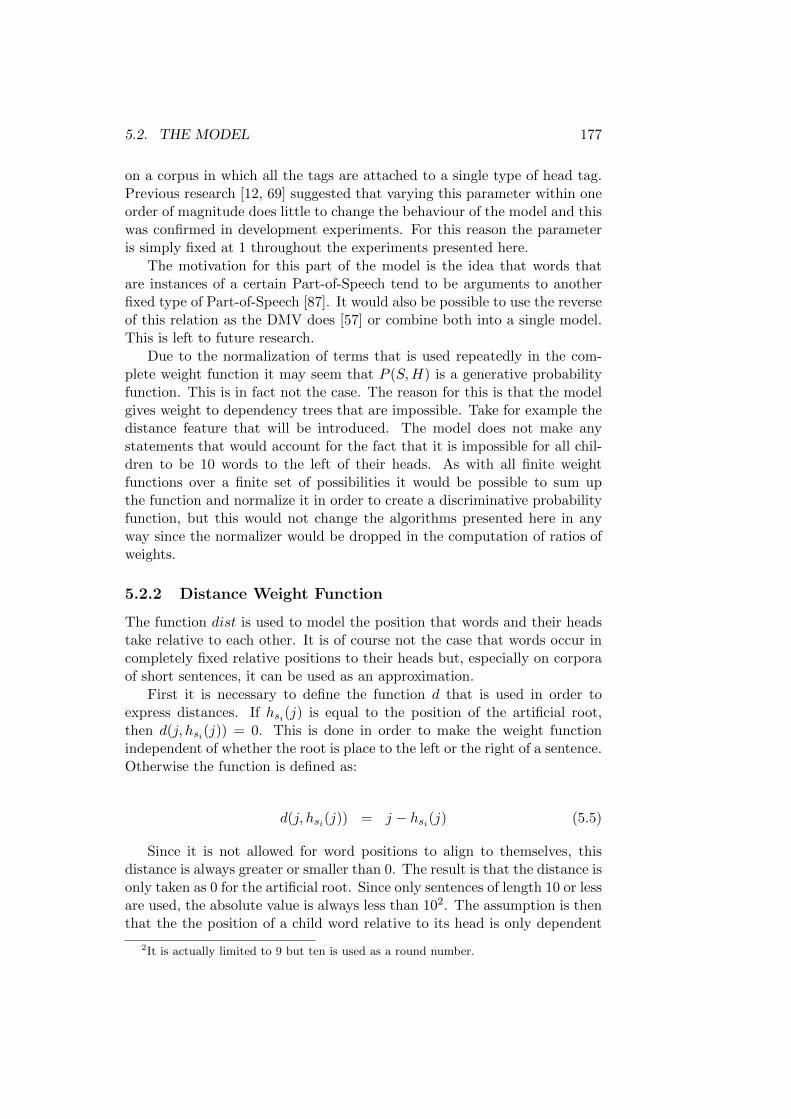
5.2. THE MODEL 177
on a corpus in which all the tags are attached to a single type of head tag.Previous research [12, 69] suggested that varying this parameter within oneorder of magnitude does little to change the behaviour of the model and thiswas confirmed in development experiments. For this reason the parameteris simply fixed at 1 throughout the experiments presented here.
The motivation for this part of the model is the idea that words thatare instances of a certain Part-of-Speech tend to be arguments to anotherfixed type of Part-of-Speech [87]. It would also be possible to use the reverseof this relation as the DMV does [57] or combine both into a single model.This is left to future research.
Due to the normalization of terms that is used repeatedly in the com-plete weight function it may seem that P (S,H) is a generative probabilityfunction. This is in fact not the case. The reason for this is that the modelgives weight to dependency trees that are impossible. Take for example thedistance feature that will be introduced. The model does not make anystatements that would account for the fact that it is impossible for all chil-dren to be 10 words to the left of their heads. As with all finite weightfunctions over a finite set of possibilities it would be possible to sum upthe function and normalize it in order to create a discriminative probabilityfunction, but this would not change the algorithms presented here in anyway since the normalizer would be dropped in the computation of ratios ofweights.
5.2.2 Distance Weight Function
The function dist is used to model the position that words and their headstake relative to each other. It is of course not the case that words occur incompletely fixed relative positions to their heads but, especially on corporaof short sentences, it can be used as an approximation.
First it is necessary to define the function d that is used in order toexpress distances. If hsi(j) is equal to the position of the artificial root,then d(j, hsi(j)) = 0. This is done in order to make the weight functionindependent of whether the root is place to the left or the right of a sentence.Otherwise the function is defined as:
d(j, hsi(j)) = j − hsi(j) (5.5)
Since it is not allowed for word positions to align to themselves, thisdistance is always greater or smaller than 0. The result is that the distance isonly taken as 0 for the artificial root. Since only sentences of length 10 or lessare used, the absolute value is always less than 102. The assumption is thenthat the the position of a child word relative to its head is only dependent
2It is actually limited to 9 but ten is used as a round number.
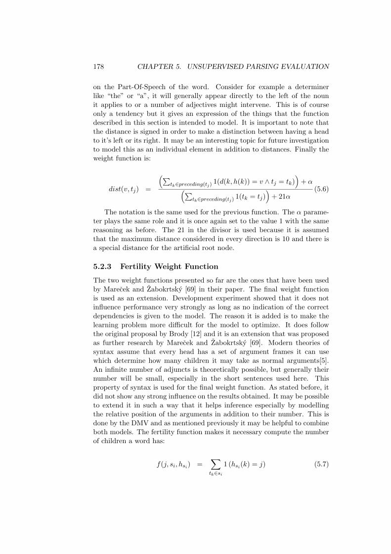
178 CHAPTER 5. UNSUPERVISED PARSING EVALUATION
on the Part-Of-Speech of the word. Consider for example a determinerlike “the” or “a”, it will generally appear directly to the left of the nounit applies to or a number of adjectives might intervene. This is of courseonly a tendency but it gives an expression of the things that the functiondescribed in this section is intended to model. It is important to note thatthe distance is signed in order to make a distinction between having a headto it’s left or its right. It may be an interesting topic for future investigationto model this as an individual element in addition to distances. Finally theweight function is:
dist(v, tj) =
(∑tk∈preceding(tj) 1(d(k, h(k)) = v ∧ tj = tk)
)+ α(∑
tk∈preceding(tj) 1(tk = tj))
+ 21α(5.6)
The notation is the same used for the previous function. The α parame-ter plays the same role and it is once again set to the value 1 with the samereasoning as before. The 21 in the divisor is used because it is assumedthat the maximum distance considered in every direction is 10 and there isa special distance for the artificial root node.
5.2.3 Fertility Weight Function
The two weight functions presented so far are the ones that have been usedby Marecek and Zabokrtsky [69] in their paper. The final weight functionis used as an extension. Development experiment showed that it does notinfluence performance very strongly as long as no indication of the correctdependencies is given to the model. The reason it is added is to make thelearning problem more difficult for the model to optimize. It does followthe original proposal by Brody [12] and it is an extension that was proposedas further research by Marecek and Zabokrtsky [69]. Modern theories ofsyntax assume that every head has a set of argument frames it can usewhich determine how many children it may take as normal arguments[5].An infinite number of adjuncts is theoretically possible, but generally theirnumber will be small, especially in the short sentences used here. Thisproperty of syntax is used for the final weight function. As stated before, itdid not show any strong influence on the results obtained. It may be possibleto extend it in such a way that it helps inference especially by modellingthe relative position of the arguments in addition to their number. This isdone by the DMV and as mentioned previously it may be helpful to combineboth models. The fertility function makes it necessary compute the numberof children a word has:
f(j, si, hsi) =∑tk∈si
1 (hsi(k) = j) (5.7)
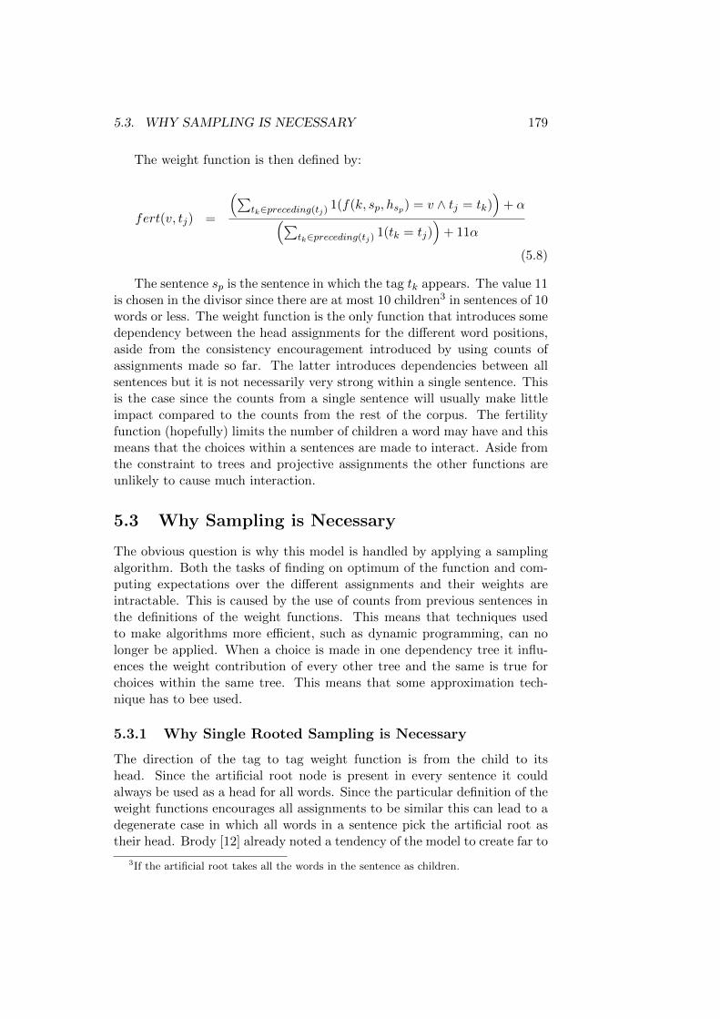
5.3. WHY SAMPLING IS NECESSARY 179
The weight function is then defined by:
fert(v, tj) =
(∑tk∈preceding(tj) 1(f(k, sp, hsp) = v ∧ tj = tk)
)+ α(∑
tk∈preceding(tj) 1(tk = tj))
+ 11α
(5.8)
The sentence sp is the sentence in which the tag tk appears. The value 11is chosen in the divisor since there are at most 10 children3 in sentences of 10words or less. The weight function is the only function that introduces somedependency between the head assignments for the different word positions,aside from the consistency encouragement introduced by using counts ofassignments made so far. The latter introduces dependencies between allsentences but it is not necessarily very strong within a single sentence. Thisis the case since the counts from a single sentence will usually make littleimpact compared to the counts from the rest of the corpus. The fertilityfunction (hopefully) limits the number of children a word may have and thismeans that the choices within a sentences are made to interact. Aside fromthe constraint to trees and projective assignments the other functions areunlikely to cause much interaction.
5.3 Why Sampling is Necessary
The obvious question is why this model is handled by applying a samplingalgorithm. Both the tasks of finding on optimum of the function and com-puting expectations over the different assignments and their weights areintractable. This is caused by the use of counts from previous sentences inthe definitions of the weight functions. This means that techniques usedto make algorithms more efficient, such as dynamic programming, can nolonger be applied. When a choice is made in one dependency tree it influ-ences the weight contribution of every other tree and the same is true forchoices within the same tree. This means that some approximation tech-nique has to bee used.
5.3.1 Why Single Rooted Sampling is Necessary
The direction of the tag to tag weight function is from the child to itshead. Since the artificial root node is present in every sentence it couldalways be used as a head for all words. Since the particular definition of theweight functions encourages all assignments to be similar this can lead to adegenerate case in which all words in a sentence pick the artificial root astheir head. Brody [12] already noted a tendency of the model to create far to
3If the artificial root takes all the words in the sentence as children.

180 CHAPTER 5. UNSUPERVISED PARSING EVALUATION
many dependency relations of this kind. The obvious way to fix this problemis to enforce a constraint on the number of root nodes a dependency treemay have. Marecek and Zabokrtsky [69] made the choice to allow only oneroot node. Since this thesis has presented a series of MCMC algorithms thatcan deal with this setting, this is the choice made here too. Therefore onlyMCMC algorithms with the single root constraint are evaluated. This hasthe side effect of evaluating all the same techniques here as were evaluatedin chapter 4.
5.4 Evaluation Setting
This section explains how the model presented in section 5.2 is used forevaluation of the sampling algorithms presented in chapter 3. The decisionsthat need to be made are the same as in chapter 4 and many of them aremade in a similar way.
5.4.1 Initialization
It has been shown that unsupervised dependency induction with the DMVis very sensitive to initialization [57, 45]. At the same time the research byMarecek and Zabokrtsky [69] and preliminary experiments suggest that theinitialization has little effect on the result of sampling the alignment modelas long as the initial structures are sufficiently randomized. This may bebecause the head choices made by the model influence each other less thenthey do in the DMV model.
Naturally the definition of random is somewhat arbitrary. The actualinitialization used is the same as in section 4.3.1 in chapter 4. All wordspick their heads randomly from among the remaining choices and the headsare picked either left to right or right to left. Non-projective samplers use anon-projective initialization and projective samplers a projective one. Theexact algorithms can be found in section 4.3.1. Note that this is similarto the initialization found to perform best by Marecek and Zabokrtsky [69]with the small caveat that their paper did not specify the notion of randomfor the random initialization.
5.4.2 Implementation of Sampling and Derivation of a Result
Sampling the complete assignments for the corpus with some algorithms awas achieved as follows:
• 3 parallel chains were used. It would have been more desirable to usemore chains but the need to store multiple head assignments for everysentence in the corpus means that the problem eventually becomesprohibitive in terms of working memory used. This is unfortunate
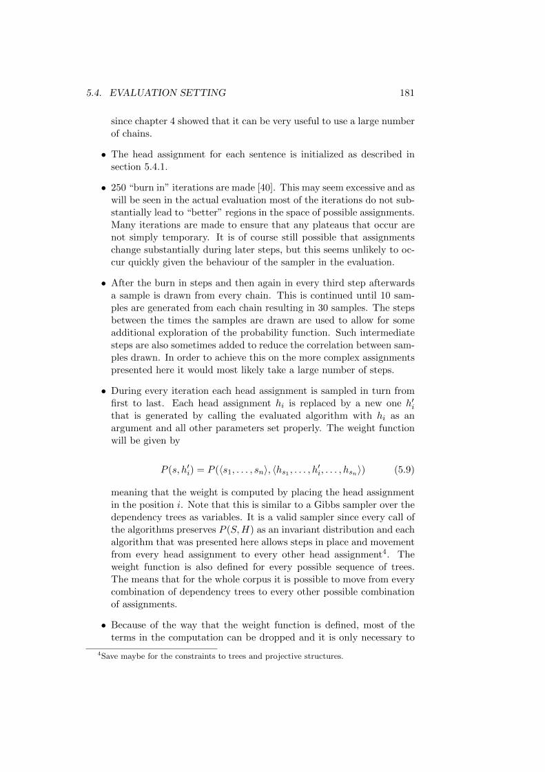
5.4. EVALUATION SETTING 181
since chapter 4 showed that it can be very useful to use a large numberof chains.
• The head assignment for each sentence is initialized as described insection 5.4.1.
• 250 “burn in” iterations are made [40]. This may seem excessive and aswill be seen in the actual evaluation most of the iterations do not sub-stantially lead to “better” regions in the space of possible assignments.Many iterations are made to ensure that any plateaus that occur arenot simply temporary. It is of course still possible that assignmentschange substantially during later steps, but this seems unlikely to oc-cur quickly given the behaviour of the sampler in the evaluation.
• After the burn in steps and then again in every third step afterwardsa sample is drawn from every chain. This is continued until 10 sam-ples are generated from each chain resulting in 30 samples. The stepsbetween the times the samples are drawn are used to allow for someadditional exploration of the probability function. Such intermediatesteps are also sometimes added to reduce the correlation between sam-ples drawn. In order to achieve this on the more complex assignmentspresented here it would most likely take a large number of steps.
• During every iteration each head assignment is sampled in turn fromfirst to last. Each head assignment hi is replaced by a new one h′ithat is generated by calling the evaluated algorithm with hi as anargument and all other parameters set properly. The weight functionwill be given by
P (s, h′i) = P (〈s1, . . . , sn〉, 〈hs1 , . . . , h′i, . . . , hsn〉) (5.9)
meaning that the weight is computed by placing the head assignmentin the position i. Note that this is similar to a Gibbs sampler over thedependency trees as variables. It is a valid sampler since every call ofthe algorithms preserves P (S,H) as an invariant distribution and eachalgorithm that was presented here allows steps in place and movementfrom every head assignment to every other head assignment4. Theweight function is also defined for every possible sequence of trees.The means that for the whole corpus it is possible to move from everycombination of dependency trees to every other possible combinationof assignments.
• Because of the way that the weight function is defined, most of theterms in the computation can be dropped and it is only necessary to
4Save maybe for the constraints to trees and projective structures.
182 CHAPTER 5. UNSUPERVISED PARSING EVALUATION
keep track of the sums that are used. In fact it would be possibleto reduce the computation of the weight ratios needed for techniquesthat sample only a single head to the inspection of two words: theone for which the head is sampled and the head assignment, sincethey are the only ones that are inspected. The latter optimization willnot be considered since it does not represent a general feature of thealgorithms, but rather is due to this specific model.
It will also be necessary to define how a final result is generated from thesampling process. Here two choices will be investigated. The first is the useof the sequence of assignments h0, . . . , hn among the ones seen during sam-pling and burn in that has the highest value of P (S,H). The second choice isan instance of minimizing the expected loss [2]. It is implemented by choos-ing as the head for each word the head it was assigned most frequently inthe 30 samples that have been drawn. This is a use of an actual expectationthat justifies the use of a sampler instead of a pure optimization algorithmbeyond the fact that samplers have been used before for this problem. Theexperimentation will show whether this leads to any improvements in theresults that are achieved. Note that the minimum of the expected loss iscomputed with respect to the loss represented by the so called unlabelledattachment score [57] and this implies that there is no consideration given towhether the resulting head assignments actually constitute trees. Marecekand Zabokrtsky [69] also tested a variant that searches for a non-projectivetree that maximizes the frequency with which its edges where seen in thesample. This will not be investigated further here.
5.4.3 Auxiliary Function
The auxiliary functions are defined relatively straightforwardly. The greedyweight function g is defined by using the weight function P as defined beforewith the single change that words that have no head assignment due to thegreedy construction are ignored both for the computation of the componentfunctions and for the determination of the counts. For the edge factoredauxiliary function the functions dist and tag are used. The counts for theother words in the sentence are ignored.
The way in which the functions are derived shows once again that thesefunctions are often easy to define. It is once again the case that the edgefactored function is much easier to compute than the the greedy auxiliaryfunction and the actual weight function. This means they will once againbe scaled by sentence length for evaluation purposes.
5.4.4 Statistics Used
The only statistics that are re-used from the evaluation in section 4.5 ofchapter 4 are the weight function evaluations and the auxiliary function
5.4. EVALUATION SETTING 183
evaluations. The functions are scaled in the same way they were previously.The amount of times that certain reference structures have been seen, aswell as the median and third quartile ratios of those reference parses arenot used. The reason for this is that it would not be clear which referenceparses to use and what ratio to expect from them. In fact there is noclear expectation that could be used to measure the quality of the samplingprocess. Instead a different statistic is used. This is the weight of thebest sequence of assignments h0, . . . , hn according to P (〈S,H〉) encounteredduring sampling. This statistic is common in the evaluation of heuristicoptimization techniques [62]. The inverse logarithm of the function is used.The logarithm is used to prevent underflow problems. The inverse to makeit possible to plot positive numbers. This implies that a small value of thisevaluation measure will be considered better.
Note that the best weight is only a weak substitute for any actual ex-pectation in terms of evaluating the performance of a sampler. It may bepossible to achieve a much better performance in terms of optimization byusing some approach specifically intended for this task such as a geneticalgorithm. A sampler is not generally intended to find the best possiblesetting of some set of parameters, although it will be encountered sooner orlater during sampling, at least if there is a finite set of possible values and asampler can be used for the task of optimization[17]. At the same time thebest weight encountered can be an indication of how well a sampler exploresthe space of possible variable settings. Since substantial weight differencesmean that certain settings are much more likely than others it would beexpected that they are encountered much earlier during sampling. If a sam-pler takes very long to reach an optimum,or reaches points that are in someway short of an optimum, then it can be expected that the sampler does notconverge very well.
Since the evaluation is done with an actual Natural Language Processingtask, part of the statistics presented should also include some performanceevaluation. This will be done by comparing the dependency parsing resultswith gold standard parses. The results of the comparison will be presentedin the form of two scores: directed accuracy and undirected accuracy. Theformer is computed by counting the times that the position of the headassigned to a word in the gold standard is equal to the position of thepredicted head. This count is then divided by the number of words in thecorpus to generate the accuracy. For the undirected accuracy the count ofcorrect heads is replace by the number of times the correct head was eitheralso the head in the predicted data or one of the children in the predicteddata. This latter measure is used since the order in a head-child relation isoften non-trivial to establish [57, 59]. Note that the undirected accuracy isalways higher that the directed version.
It would of course be interesting to extend the evaluation to some moreapplied task but there is a lack of a well establish tasks that can be used to
184 CHAPTER 5. UNSUPERVISED PARSING EVALUATION
for this[96, 59]. Therefore this addition is kept for future research.
5.5 Data Used
As a last step before any evaluation can be presented it is necessary topresent the input data and the way that there corpora are prepared. TheWorkshop on The Induction of Linguistic Structures was held in 2012 andpart of the workshop were shared tasks on the induction of dependencytrees and/or Part-of-Speech Tags. Along with the task a set of corporawas published, some of which are publicly available. The publicly availablecorpora are the ones used here. These are [45]:
• The Basque 3lb Dependency Treebank
• The Danish Copenhagen Dependency Treebank
• The Dutch Alpino treebank
• The Portuguese Floresta Sinta(c)tica Treebank
• The English CHILDES US/Brown Subcorpus
• The Swedish Talbanken Treebank
• The Slovene jos500k Treebank
all the corpora are converted to a special format for the workshop task.For more information consult the overview paper by Gelling et. al. [45]. Inthe following the different corpora will be referred to simply by the languagethey represent a sample from. Note that the CHILDES English corpus isvery dissimilar from the other corpora since it is taken from conversationsbetween parents and their children. The corpora are provided with a train-ing, development and testing split of the data. Since training is supposed tonot make any use of dependency information from the corpora it was stan-dard practice for the challenge to use all the data in the final run and thenmake an evaluation against the gold standard dependencies in the test set.The development set is intended to tune parameters and test out differentsettings, which is exactly what it was used for during the preparation of theresults presented here. The final results where then derived on the test set.
It is a common difficulty reduction technique to only consider sentencesof length 10 or shorter for unsupervised tasks in parsing [57, 69, 45] andpunctuation is dropped for both training and evaluation since the handlingof punctuation is often a rather arbitrary decision during the development oftreebanks. The performance of the model presented here is compared againstthe other results from the WILS task. This means that all choices are madein the same way as they were for the workshop. The decision whether a
5.6. PURE ALIGNMENT MODEL 185
sentence is of length 10 or less is made before punctuation is removed. Thecorpora are provided with a universal tag set that was developed by Petrovet. al. [86]. The universal tags are used to decide which words to removeas punctuation. All words that are tagged with the universal tag “.” areremoved both for the sampling process and for evaluation. If a word in thegold standard dependencies is attached at a removed word w, then its headis changed to the head of w. If this new head is also removed, then it isattached to the head of that word and so on until a word that has not beenremoved is reached or the process stops at the artificial root node.
5.6 Pure Alignment Model
Throughout the evaluations presented here coarse Part-Of-Speech tags areused. As stated before, the corpora also provide universal POS tags thatare identical for all the languages. These tags are computed automaticallywith a tool that Petrov et. al. developed [86]. The reason these tags arenot used is the fact that they are a reduction of information from the coarsePart-Of-Speech tags used to compute them. There are also some instancesin which the universal tags are somewhat suspicious. Two examples of thisis the unusually high number of words tagged “X” in the reduced corpusfor Basque. “X” is the tag used for miscellaneous and should not be asfrequent in the corpus. The universal tagging also has an influence on thetask presented here. In the Danish corpus a large number of punctuationmarks are assigned the universal tag “X” and are therefore not removed inthe reduction of the corpora which is based on the universal “.” tag.
The corpora also provide a fine grained POS tag for every word in thecorpus. This tag is only different in from the coarse POS tag for some ofthe corpora. Where it is provided it can be so fine grained that it does notremove the problem of data sparsity.
The evaluation in this section proceeds as follows. For every languagethe curves for the weight function after a certain number of iterations arepresented. They are more or less all similar across languages and thereare some general tendencies that can be derived from them. There aresome interesting deviations in behaviour for some languages. For Basqueand Danish the numbers of weight and auxiliary function evaluations areplotted. The plots for other languages would be similar up to some scalingfor the number of sentences in a corpus. The ordering of relative sizes ofthe graphs are similar to what was observed in chapter 4. Therefore thepresentation of the function evaluations is reduced somewhat in order tosave space. In the number of evaluation there was also an overflow problemfor the larger corpora.
After a discussion of the convergence behaviour of the different samplingalgorithms a presentation of the performance in terms of an comparison to
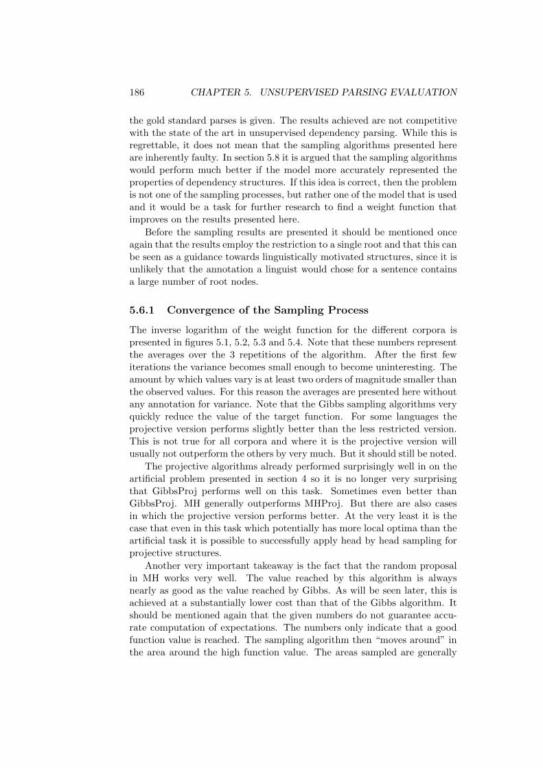
186 CHAPTER 5. UNSUPERVISED PARSING EVALUATION
the gold standard parses is given. The results achieved are not competitivewith the state of the art in unsupervised dependency parsing. While this isregrettable, it does not mean that the sampling algorithms presented hereare inherently faulty. In section 5.8 it is argued that the sampling algorithmswould perform much better if the model more accurately represented theproperties of dependency structures. If this idea is correct, then the problemis not one of the sampling processes, but rather one of the model that is usedand it would be a task for further research to find a weight function thatimproves on the results presented here.
Before the sampling results are presented it should be mentioned onceagain that the results employ the restriction to a single root and that this canbe seen as a guidance towards linguistically motivated structures, since it isunlikely that the annotation a linguist would chose for a sentence containsa large number of root nodes.
5.6.1 Convergence of the Sampling Process
The inverse logarithm of the weight function for the different corpora ispresented in figures 5.1, 5.2, 5.3 and 5.4. Note that these numbers representthe averages over the 3 repetitions of the algorithm. After the first fewiterations the variance becomes small enough to become uninteresting. Theamount by which values vary is at least two orders of magnitude smaller thanthe observed values. For this reason the averages are presented here withoutany annotation for variance. Note that the Gibbs sampling algorithms veryquickly reduce the value of the target function. For some languages theprojective version performs slightly better than the less restricted version.This is not true for all corpora and where it is the projective version willusually not outperform the others by very much. But it should still be noted.
The projective algorithms already performed surprisingly well in on theartificial problem presented in section 4 so it is no longer very surprisingthat GibbsProj performs well on this task. Sometimes even better thanGibbsProj. MH generally outperforms MHProj. But there are also casesin which the projective version performs better. At the very least it is thecase that even in this task which potentially has more local optima than theartificial task it is possible to successfully apply head by head sampling forprojective structures.
Another very important takeaway is the fact that the random proposalin MH works very well. The value reached by this algorithm is alwaysnearly as good as the value reached by Gibbs. As will be seen later, this isachieved at a substantially lower cost than that of the Gibbs algorithm. Itshould be mentioned again that the given numbers do not guarantee accu-rate computation of expectations. The numbers only indicate that a goodfunction value is reached. The sampling algorithm then “moves around” inthe area around the high function value. The areas sampled are generally
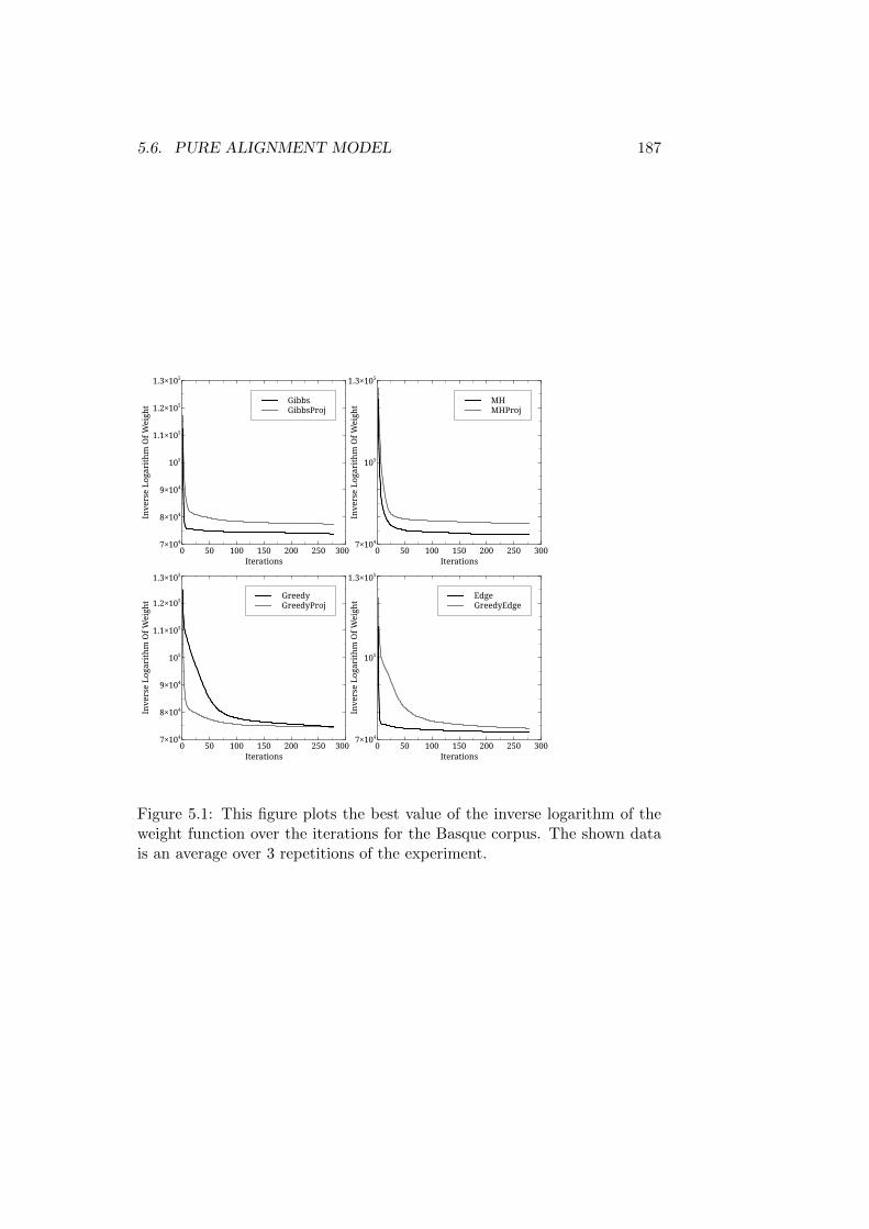
5.6. PURE ALIGNMENT MODEL 187
GibbsGibbsProj
Inve
rse
Loga
rith
m O
f Wei
ght
7×10⁴
8×10⁴
9×10⁴
105
1.1×10⁵
1.2×10⁵
1.3×10⁵
Iterations0 50 100 150 200 250 300
MHMHProj
Inve
rse
Loga
rith
m O
f Wei
ght
7×10⁴
105
1.3×10⁵
Iterations0 50 100 150 200 250 300
GreedyGreedyProj
Inve
rse
Loga
rith
m O
f Wei
ght
7×10⁴
8×10⁴
9×10⁴
105
1.1×10⁵
1.2×10⁵
1.3×10⁵
Iterations0 50 100 150 200 250 300
EdgeGreedyEdge
Inve
rse
Loga
rith
m O
f Wei
ght
7×10⁴
105
1.3×10⁵
Iterations0 50 100 150 200 250 300
Figure 5.1: This figure plots the best value of the inverse logarithm of theweight function over the iterations for the Basque corpus. The shown datais an average over 3 repetitions of the experiment.
188 CHAPTER 5. UNSUPERVISED PARSING EVALUATION
GibbsGibbsProj
Inve
rse
Loga
rith
m O
f Wei
ght
3×10⁴
3.5×10⁴
4×10⁴
4.5×10⁴
5×10⁴
5.5×10⁴
Iterations0 50 100 150 200 250 300
MHMHProj
Inve
rse
Loga
rith
m O
f Wei
ght
3×10⁴
5.5×10⁴
Iterations0 50 100 150 200 250 300
GreedyGreedyProj
Inve
rse
Loga
rith
m O
f Wei
ght
3×10⁴
3.5×10⁴
4×10⁴
4.5×10⁴
5×10⁴
5.5×10⁴
Iterations0 50 100 150 200 250 300
EdgeGreedyEdge
Inve
rse
Loga
rith
m O
f Wei
ght
3×10⁴
5.5×10⁴
Iterations0 50 100 150 200 250 300
Figure 5.2: This figure plots the best value of the inverse logarithm of theweight function over the iterations for the Danish Corpus in the upper figureand the Dutch corpus in the lower one. The shown data is an average over3 repetitions of the experiment.
5.6. PURE ALIGNMENT MODEL 189
better than the intermediate assignments by a substantial amount. Thisalso means they should be visited substantially more often during MCMCsteps in order for the better structures to be represented by an appropriateamount. The discovery of high weight areas can indicate that the samplebecomes more representative by increasing the number of times that theseareas occur in the generated structures.
The results presented are less encouraging for Greedy and GreedyEdge.They reach good values slower and the values they reach are worse. Whileit would be possible that this is because a preliminary optimum is reachedwhen the whole structures are sampled at once, it seems far more likelythat this is caused by the root sampling step. The two algorithms sampletheir roots only during the greedy global step they make. Both Edge andGreedyProj do not have a similar problem. The current conclusion that canbe drawn from these results is that with the auxiliary function defined as itis, finding a root is difficult. In future experiments it would be of interestto add root sampling steps for MH and Gibbs to the Greedy algorithm.
The question is then whether this combination could perform as well asthe GreedyProj algorithm. The algorithm reaches the best function valuesin all the languages. It outperforms GibbsProj which it extends by a greedyglobal sampling step. It is interesting that this global step seems to havesome effect on the quality of the results. The global step in Edge has nonoticeable positive effect on the performance of the algorithm compared tothe basis of Gibbs on which it improves. This is most likely the case sincethe single edge approximation used is so close to correctness in this case thatthe Gibbs sampler can also work well with its word by word updates.
All the statements made so far only describe how well the MCMC schemesdo in obtaining good function values. It is of course also of interest to knowhow much resources have to be expended in order to achieve these results.Figure 5.5 shows the number of function evaluation used. They are scaled bythe sentence lengths. As stated before, in order to compute the values it isonly necessary to keep counts from the other sentences and then inspect thehead assignments currently sampled. This means that when a head assign-ment for a sentence of length n is sampled and the weight function evaluated,then n will be added to the number of evaluations. This makes the resultscomparable to the edge factored auxiliary evaluations that only inspect asingle edge. It also means that longer sentences that make a larger contri-bution to the computation time during function evaluations are representedaccordingly in the graph.
The results on the function evaluations are in line with what was seenin chapter 4. The Gibbs root sampling steps are the most expensive partof the process. The use of the restriction to projective structures bringssomething of a reduction in the number of function evaluations that areneeded. It should be noted that the MH and MHProj algorithms use areduced number of function evaluations to achieve their performance.
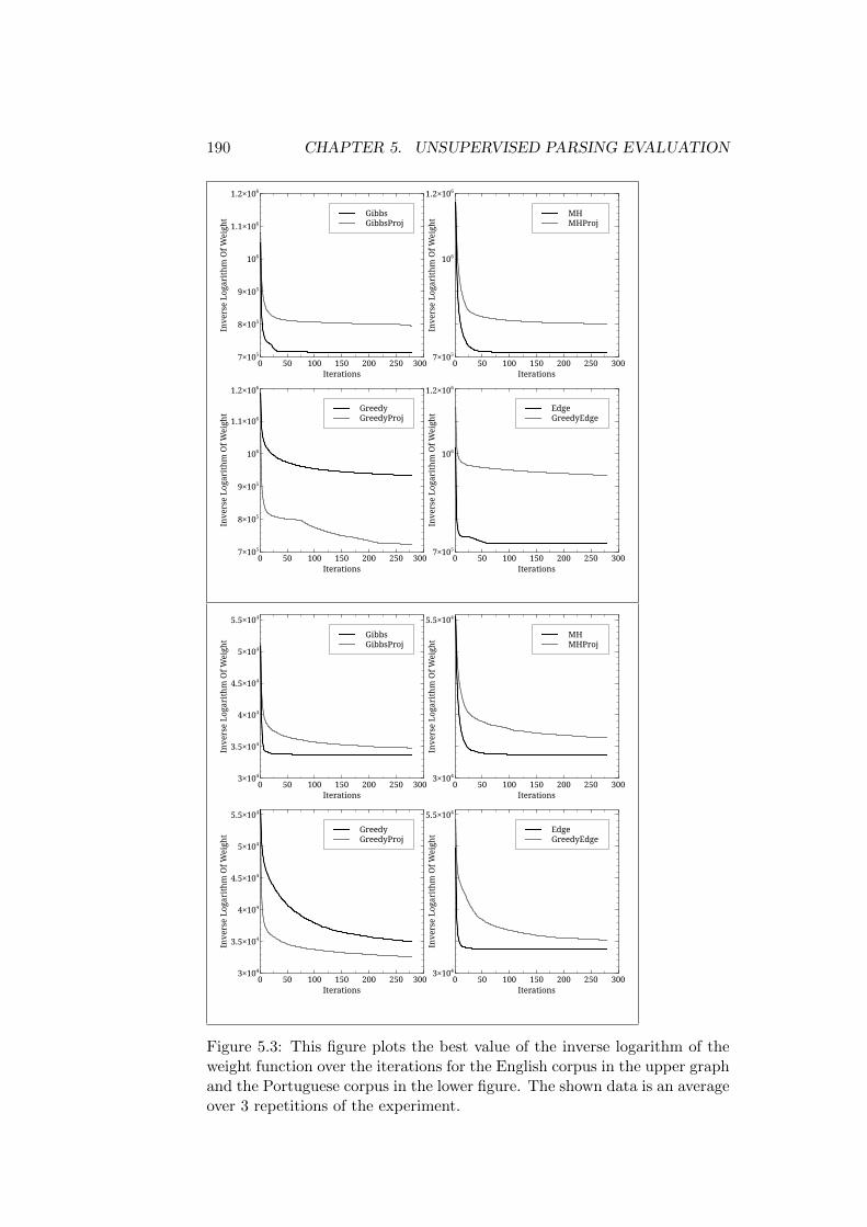
190 CHAPTER 5. UNSUPERVISED PARSING EVALUATION
GibbsGibbsProj
Inve
rse
Loga
rith
m O
f Wei
ght
7×10⁵
8×10⁵
9×10⁵
106
1.1×10⁶
1.2×10⁶
Iterations0 50 100 150 200 250 300
MHMHProj
Inve
rse
Loga
rith
m O
f Wei
ght
7×10⁵
106
1.2×10⁶
Iterations0 50 100 150 200 250 300
GreedyGreedyProj
Inve
rse
Loga
rith
m O
f Wei
ght
7×10⁵
8×10⁵
9×10⁵
106
1.1×10⁶
1.2×10⁶
Iterations0 50 100 150 200 250 300
EdgeGreedyEdge
Inve
rse
Loga
rith
m O
f Wei
ght
7×10⁵
106
1.2×10⁶
Iterations0 50 100 150 200 250 300
GibbsGibbsProj
Inve
rse
Loga
rith
m O
f Wei
ght
3×10⁴
3.5×10⁴
4×10⁴
4.5×10⁴
5×10⁴
5.5×10⁴
Iterations0 50 100 150 200 250 300
MHMHProj
Inve
rse
Loga
rith
m O
f Wei
ght
3×10⁴
5.5×10⁴
Iterations0 50 100 150 200 250 300
GreedyGreedyProj
Inve
rse
Loga
rith
m O
f Wei
ght
3×10⁴
3.5×10⁴
4×10⁴
4.5×10⁴
5×10⁴
5.5×10⁴
Iterations0 50 100 150 200 250 300
EdgeGreedyEdge
Inve
rse
Loga
rith
m O
f Wei
ght
3×10⁴
5.5×10⁴
Iterations0 50 100 150 200 250 300
Figure 5.3: This figure plots the best value of the inverse logarithm of theweight function over the iterations for the English corpus in the upper graphand the Portuguese corpus in the lower figure. The shown data is an averageover 3 repetitions of the experiment.
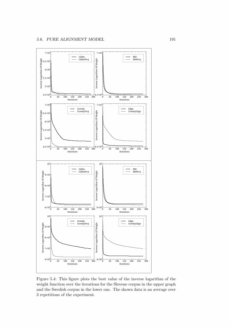
5.6. PURE ALIGNMENT MODEL 191
GibbsGibbsProj
Inve
rse
Loga
rith
m O
f Wei
ght
4.5×10⁴
5×10⁴
5.5×10⁴
6×10⁴
6.5×10⁴
7×10⁴
Iterations0 50 100 150 200 250 300
MHMHProj
Inve
rse
Loga
rith
m O
f Wei
ght
4.5×10⁴
7×10⁴
Iterations0 50 100 150 200 250 300
GreedyGreedyProj
Inve
rse
Loga
rith
m O
f Wei
ght
4.5×10⁴
5×10⁴
5.5×10⁴
6×10⁴
6.5×10⁴
7×10⁴
Iterations0 50 100 150 200 250 300
EdgeGreedyEdge
Inve
rse
Loga
rith
m O
f Wei
ght
4.5×10⁴
7×10⁴
Iterations0 50 100 150 200 250 300
GibbsGibbsProj
Inve
rse
Loga
rith
m O
f Wei
ght
6×10⁴
7×10⁴
8×10⁴
9×10⁴
105
Iterations0 50 100 150 200 250 300
MHMHProj
Inve
rse
Loga
rith
m O
f Wei
ght
6×10⁴
105
Iterations0 50 100 150 200 250 300
GreedyGreedyProj
Inve
rse
Loga
rith
m O
f Wei
ght
6×10⁴
7×10⁴
8×10⁴
9×10⁴
105
Iterations0 50 100 150 200 250 300
EdgeGreedyEdge
Inve
rse
Loga
rith
m O
f Wei
ght
6×10⁴
105
Iterations0 50 100 150 200 250 300
Figure 5.4: This figure plots the best value of the inverse logarithm of theweight function over the iterations for the Slovene corpus in the upper graphand the Swedish corpus in the lower one. The shown data is an average over3 repetitions of the experiment.
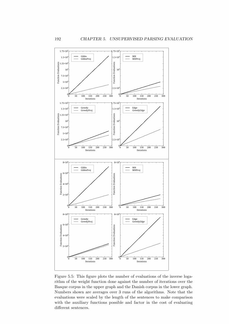
192 CHAPTER 5. UNSUPERVISED PARSING EVALUATION
GibbsGibbsProj
Func
tion
Eva
luat
ions
0
2.5×10⁸
5×10⁸
7.5×10⁸
109
1.25×10⁹
1.5×10⁹
1.75×10⁹
Iterations0 50 100 150 200 250 300
MHMHProj
Func
tion
Eva
luat
ions
0
2.5×10⁸
109
1.5×10⁹
1.75×10⁹
Iterations0 50 100 150 200 250 300
GreedyGreedyProj
Func
tion
Eva
luat
ions
0
2.5×10⁸
5×10⁸
7.5×10⁸
109
1.25×10⁹
1.5×10⁹
1.75×10⁹
Iterations0 50 100 150 200 250 300
EdgeGreedyEdge
Func
tion
Eva
luat
ions
0
2.5×10⁸
109
1.5×10⁹
1.75×10⁹
Iterations0 50 100 150 200 250 300
GibbsGibbsProj
Func
tion
Eva
luat
ions
0
2×10⁸
4×10⁸
6×10⁸
8×10⁸
Iterations0 50 100 150 200 250 300
MHMHProj
Func
tion
Eva
luat
ions
0
8×10⁸
Iterations0 50 100 150 200 250 300
GreedyGreedyProj
Func
tion
Eva
luat
ions
0
2×10⁸
4×10⁸
6×10⁸
8×10⁸
Iterations0 50 100 150 200 250 300
EdgeGreedyEdge
Func
tion
Eva
luat
ions
0
8×10⁸
Iterations0 50 100 150 200 250 300
Figure 5.5: This figure plots the number of evaluations of the inverse loga-rithm of the weight function done against the number of iterations over theBasque corpus in the upper graph and the Danish corpus in the lower graph.Numbers shown are averages over 3 runs of the algorithms. Note that theevaluations were scaled by the length of the sentences to make comparisonwith the auxiliary functions possible and factor in the cost of evaluatingdifferent sentences.

5.6. PURE ALIGNMENT MODEL 193
EdgeGreedyEdge
Aux
iliar
y Ev
alua
tion
s
0
2.5×10⁸
5×10⁸
7.5×10⁸
109
1.25×10⁹
1.5×10⁹
1.75×10⁹
Iterations0 50 100 150 200 250 300
GreedyGreedyProj
Aux
iliar
y Ev
alua
tion
s
0
2.5×10⁸
109
1.5×10⁹
1.75×10⁹
Iterations0 50 100 150 200 250 300
EdgeGreedyEdge
Aux
iliar
y Ev
alua
tion
s
0
2×10⁸
4×10⁸
6×10⁸
8×10⁸
Iterations0 50 100 150 200 250 300
GreedyGreedyProj
Aux
iliar
y Ev
alua
tion
s
0
2×10⁸
6×10⁸
8×10⁸
Iterations0 50 100 150 200 250 300
Figure 5.6: Plot that shows the amount of auxiliary function evaluationsmade up to a certain number of iterations over the Basque corpus in theupper graph and the Danish corpus in the lower graph. Shown is the averageover 3 repetitions. Note that the greedy auxiliary function evaluations arescaled by the length of the sentences. This is done to make a comparisonwith the Edge factored function possible.
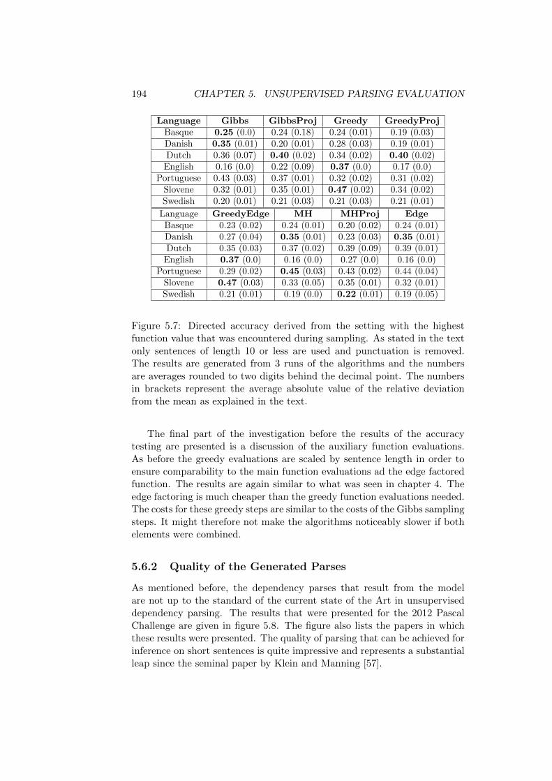
194 CHAPTER 5. UNSUPERVISED PARSING EVALUATION
Language Gibbs GibbsProj Greedy GreedyProjBasque 0.25 (0.0) 0.24 (0.18) 0.24 (0.01) 0.19 (0.03)Danish 0.35 (0.01) 0.20 (0.01) 0.28 (0.03) 0.19 (0.01)Dutch 0.36 (0.07) 0.40 (0.02) 0.34 (0.02) 0.40 (0.02)
English 0.16 (0.0) 0.22 (0.09) 0.37 (0.0) 0.17 (0.0)Portuguese 0.43 (0.03) 0.37 (0.01) 0.32 (0.02) 0.31 (0.02)
Slovene 0.32 (0.01) 0.35 (0.01) 0.47 (0.02) 0.34 (0.02)Swedish 0.20 (0.01) 0.21 (0.03) 0.21 (0.03) 0.21 (0.01)
Language GreedyEdge MH MHProj EdgeBasque 0.23 (0.02) 0.24 (0.01) 0.20 (0.02) 0.24 (0.01)Danish 0.27 (0.04) 0.35 (0.01) 0.23 (0.03) 0.35 (0.01)Dutch 0.35 (0.03) 0.37 (0.02) 0.39 (0.09) 0.39 (0.01)
English 0.37 (0.0) 0.16 (0.0) 0.27 (0.0) 0.16 (0.0)Portuguese 0.29 (0.02) 0.45 (0.03) 0.43 (0.02) 0.44 (0.04)
Slovene 0.47 (0.03) 0.33 (0.05) 0.35 (0.01) 0.32 (0.01)Swedish 0.21 (0.01) 0.19 (0.0) 0.22 (0.01) 0.19 (0.05)
Figure 5.7: Directed accuracy derived from the setting with the highestfunction value that was encountered during sampling. As stated in the textonly sentences of length 10 or less are used and punctuation is removed.The results are generated from 3 runs of the algorithms and the numbersare averages rounded to two digits behind the decimal point. The numbersin brackets represent the average absolute value of the relative deviationfrom the mean as explained in the text.
The final part of the investigation before the results of the accuracytesting are presented is a discussion of the auxiliary function evaluations.As before the greedy evaluations are scaled by sentence length in order toensure comparability to the main function evaluations ad the edge factoredfunction. The results are again similar to what was seen in chapter 4. Theedge factoring is much cheaper than the greedy function evaluations needed.The costs for these greedy steps are similar to the costs of the Gibbs samplingsteps. It might therefore not make the algorithms noticeably slower if bothelements were combined.
5.6.2 Quality of the Generated Parses
As mentioned before, the dependency parses that result from the modelare not up to the standard of the current state of the Art in unsuperviseddependency parsing. The results that were presented for the 2012 PascalChallenge are given in figure 5.8. The figure also lists the papers in whichthese results were presented. The quality of parsing that can be achieved forinference on short sentences is quite impressive and represents a substantialleap since the seminal paper by Klein and Manning [57].
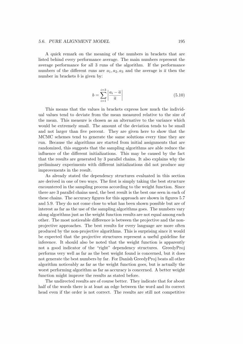
5.6. PURE ALIGNMENT MODEL 195
A quick remark on the meaning of the numbers in brackets that arelisted behind every performance average. The main numbers represent theaverage performance for all 3 runs of the algorithm. If the performancenumbers of the different runs are a1, a2, a3 and the average is a then thenumber in brackets b is given by:
b =i=3∑i=1
∣∣∣∣ai − aa
∣∣∣∣ (5.10)
This means that the values in brackets express how much the individ-ual values tend to deviate from the mean measured relative to the size ofthe mean. This measure is chosen as an alternative to the variance whichwould be extremely small. The amount of the deviation tends to be smalland not larger than five percent. They are given here to show that theMCMC schemes tend to generate the same solutions every time they arerun. Because the algorithms are started from initial assignments that arerandomized, this suggests that the sampling algorithms are able reduce theinfluence of the different initializations. This may be caused by the factthat the results are generated by 3 parallel chains. It also explains why thepreliminary experiments with different initializations did not produce anyimprovements in the result.
As already stated the dependency structures evaluated in this sectionare derived in one of two ways. The first is simply taking the best structureencountered in the sampling process according to the weight function. Sincethere are 3 parallel chains used, the best result is the best one seen in each ofthese chains. The accuracy figures for this approach are shown in figures 5.7and 5.9. They do not come close to what has been shown possible but are ofinterest as far as the use of the sampling algorithms goes. The numbers varyalong algorithms just as the weight function results are not equal among eachother. The most noticeable difference is between the projective and the non-projective approaches. The best results for every language are more oftenproduced by the non-projective algorithms. This is surprising since it wouldbe expected that the projective structures represent a useful guideline forinference. It should also be noted that the weight function is apparentlynot a good indicator of the “right” dependency structures. GreedyProjperforms very well as far as the best weight found is concerned, but it doesnot generate the best numbers by far. For Danish GreedyProj beats all otheralgorithm noticeably as far as the weight function goes, but is actually theworst performing algorithm as far as accuracy is concerned. A better weightfunction might improve the results as stated before.
The undirected results are of course better. They indicate that for abouthalf of the words there is at least an edge between the word and its correcthead even if the order is not correct. The results are still not competitive
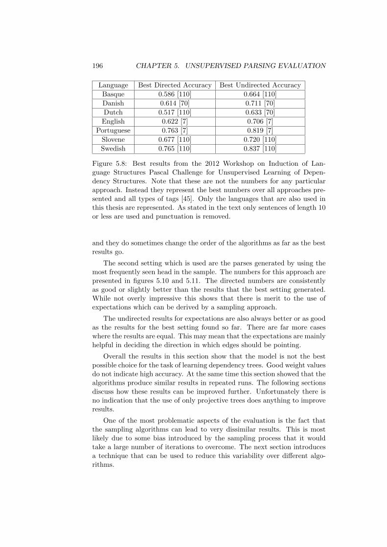
196 CHAPTER 5. UNSUPERVISED PARSING EVALUATION
Language Best Directed Accuracy Best Undirected Accuracy
Basque 0.586 [110] 0.664 [110]
Danish 0.614 [70] 0.711 [70]
Dutch 0.517 [110] 0.633 [70]
English 0.622 [7] 0.706 [7]
Portuguese 0.763 [7] 0.819 [7]
Slovene 0.677 [110] 0.720 [110]
Swedish 0.765 [110] 0.837 [110]
Figure 5.8: Best results from the 2012 Workshop on Induction of Lan-guage Structures Pascal Challenge for Unsupervised Learning of Depen-dency Structures. Note that these are not the numbers for any particularapproach. Instead they represent the best numbers over all approaches pre-sented and all types of tags [45]. Only the languages that are also used inthis thesis are represented. As stated in the text only sentences of length 10or less are used and punctuation is removed.
and they do sometimes change the order of the algorithms as far as the bestresults go.
The second setting which is used are the parses generated by using themost frequently seen head in the sample. The numbers for this approach arepresented in figures 5.10 and 5.11. The directed numbers are consistentlyas good or slightly better than the results that the best setting generated.While not overly impressive this shows that there is merit to the use ofexpectations which can be derived by a sampling approach.
The undirected results for expectations are also always better or as goodas the results for the best setting found so far. There are far more caseswhere the results are equal. This may mean that the expectations are mainlyhelpful in deciding the direction in which edges should be pointing.
Overall the results in this section show that the model is not the bestpossible choice for the task of learning dependency trees. Good weight valuesdo not indicate high accuracy. At the same time this section showed that thealgorithms produce similar results in repeated runs. The following sectionsdiscuss how these results can be improved further. Unfortunately there isno indication that the use of only projective trees does anything to improveresults.
One of the most problematic aspects of the evaluation is the fact thatthe sampling algorithms can lead to very dissimilar results. This is mostlikely due to some bias introduced by the sampling process that it wouldtake a large number of iterations to overcome. The next section introducesa technique that can be used to reduce this variability over different algo-rithms.
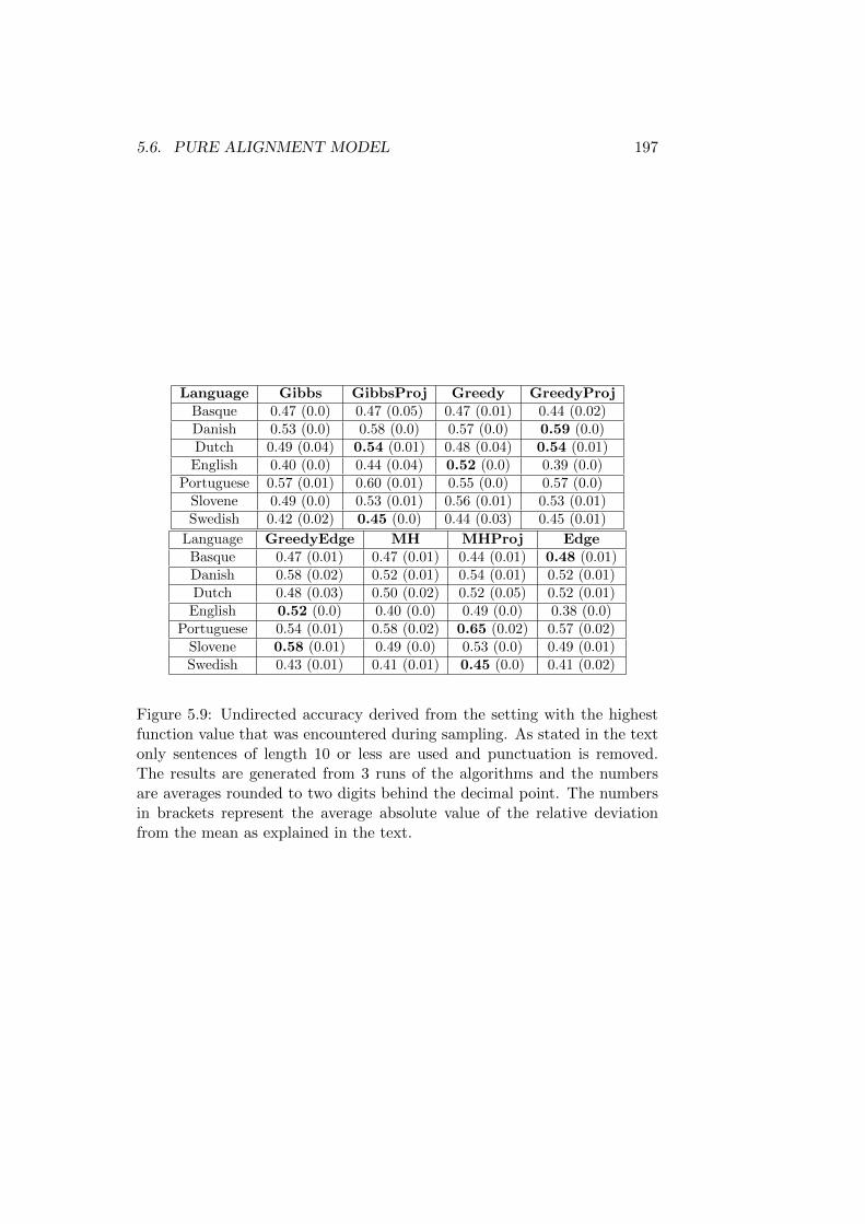
5.6. PURE ALIGNMENT MODEL 197
Language Gibbs GibbsProj Greedy GreedyProjBasque 0.47 (0.0) 0.47 (0.05) 0.47 (0.01) 0.44 (0.02)Danish 0.53 (0.0) 0.58 (0.0) 0.57 (0.0) 0.59 (0.0)Dutch 0.49 (0.04) 0.54 (0.01) 0.48 (0.04) 0.54 (0.01)
English 0.40 (0.0) 0.44 (0.04) 0.52 (0.0) 0.39 (0.0)Portuguese 0.57 (0.01) 0.60 (0.01) 0.55 (0.0) 0.57 (0.0)
Slovene 0.49 (0.0) 0.53 (0.01) 0.56 (0.01) 0.53 (0.01)Swedish 0.42 (0.02) 0.45 (0.0) 0.44 (0.03) 0.45 (0.01)
Language GreedyEdge MH MHProj EdgeBasque 0.47 (0.01) 0.47 (0.01) 0.44 (0.01) 0.48 (0.01)Danish 0.58 (0.02) 0.52 (0.01) 0.54 (0.01) 0.52 (0.01)Dutch 0.48 (0.03) 0.50 (0.02) 0.52 (0.05) 0.52 (0.01)
English 0.52 (0.0) 0.40 (0.0) 0.49 (0.0) 0.38 (0.0)Portuguese 0.54 (0.01) 0.58 (0.02) 0.65 (0.02) 0.57 (0.02)
Slovene 0.58 (0.01) 0.49 (0.0) 0.53 (0.0) 0.49 (0.01)Swedish 0.43 (0.01) 0.41 (0.01) 0.45 (0.0) 0.41 (0.02)
Figure 5.9: Undirected accuracy derived from the setting with the highestfunction value that was encountered during sampling. As stated in the textonly sentences of length 10 or less are used and punctuation is removed.The results are generated from 3 runs of the algorithms and the numbersare averages rounded to two digits behind the decimal point. The numbersin brackets represent the average absolute value of the relative deviationfrom the mean as explained in the text.
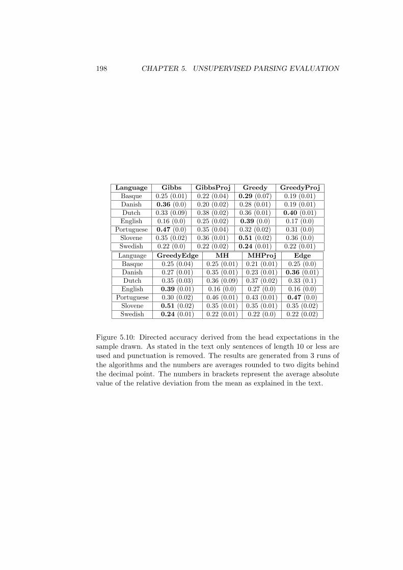
198 CHAPTER 5. UNSUPERVISED PARSING EVALUATION
Language Gibbs GibbsProj Greedy GreedyProjBasque 0.25 (0.01) 0.22 (0.04) 0.29 (0.07) 0.19 (0.01)Danish 0.36 (0.0) 0.20 (0.02) 0.28 (0.01) 0.19 (0.01)Dutch 0.33 (0.09) 0.38 (0.02) 0.36 (0.01) 0.40 (0.01)
English 0.16 (0.0) 0.25 (0.02) 0.39 (0.0) 0.17 (0.0)Portuguese 0.47 (0.0) 0.35 (0.04) 0.32 (0.02) 0.31 (0.0)
Slovene 0.35 (0.02) 0.36 (0.01) 0.51 (0.02) 0.36 (0.0)Swedish 0.22 (0.0) 0.22 (0.02) 0.24 (0.01) 0.22 (0.01)
Language GreedyEdge MH MHProj EdgeBasque 0.25 (0.04) 0.25 (0.01) 0.21 (0.01) 0.25 (0.0)Danish 0.27 (0.01) 0.35 (0.01) 0.23 (0.01) 0.36 (0.01)Dutch 0.35 (0.03) 0.36 (0.09) 0.37 (0.02) 0.33 (0.1)
English 0.39 (0.01) 0.16 (0.0) 0.27 (0.0) 0.16 (0.0)Portuguese 0.30 (0.02) 0.46 (0.01) 0.43 (0.01) 0.47 (0.0)
Slovene 0.51 (0.02) 0.35 (0.01) 0.35 (0.01) 0.35 (0.02)Swedish 0.24 (0.01) 0.22 (0.01) 0.22 (0.0) 0.22 (0.02)
Figure 5.10: Directed accuracy derived from the head expectations in thesample drawn. As stated in the text only sentences of length 10 or less areused and punctuation is removed. The results are generated from 3 runs ofthe algorithms and the numbers are averages rounded to two digits behindthe decimal point. The numbers in brackets represent the average absolutevalue of the relative deviation from the mean as explained in the text.
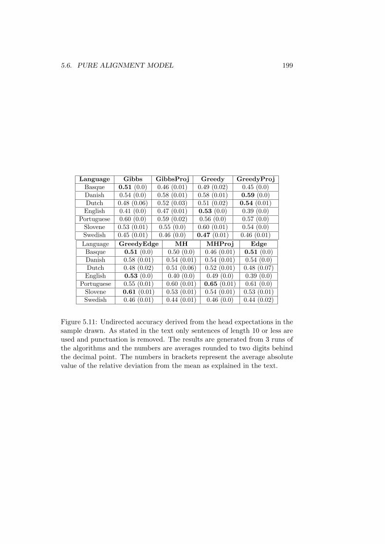
5.6. PURE ALIGNMENT MODEL 199
Language Gibbs GibbsProj Greedy GreedyProjBasque 0.51 (0.0) 0.46 (0.01) 0.49 (0.02) 0.45 (0.0)Danish 0.54 (0.0) 0.58 (0.01) 0.58 (0.01) 0.59 (0.0)Dutch 0.48 (0.06) 0.52 (0.03) 0.51 (0.02) 0.54 (0.01)
English 0.41 (0.0) 0.47 (0.01) 0.53 (0.0) 0.39 (0.0)Portuguese 0.60 (0.0) 0.59 (0.02) 0.56 (0.0) 0.57 (0.0)
Slovene 0.53 (0.01) 0.55 (0.0) 0.60 (0.01) 0.54 (0.0)Swedish 0.45 (0.01) 0.46 (0.0) 0.47 (0.01) 0.46 (0.01)
Language GreedyEdge MH MHProj EdgeBasque 0.51 (0.0) 0.50 (0.0) 0.46 (0.01) 0.51 (0.0)Danish 0.58 (0.01) 0.54 (0.01) 0.54 (0.01) 0.54 (0.0)Dutch 0.48 (0.02) 0.51 (0.06) 0.52 (0.01) 0.48 (0.07)
English 0.53 (0.0) 0.40 (0.0) 0.49 (0.0) 0.39 (0.0)Portuguese 0.55 (0.01) 0.60 (0.01) 0.65 (0.01) 0.61 (0.0)
Slovene 0.61 (0.01) 0.53 (0.01) 0.54 (0.01) 0.53 (0.01)Swedish 0.46 (0.01) 0.44 (0.01) 0.46 (0.0) 0.44 (0.02)
Figure 5.11: Undirected accuracy derived from the head expectations in thesample drawn. As stated in the text only sentences of length 10 or less areused and punctuation is removed. The results are generated from 3 runs ofthe algorithms and the numbers are averages rounded to two digits behindthe decimal point. The numbers in brackets represent the average absolutevalue of the relative deviation from the mean as explained in the text.

200 CHAPTER 5. UNSUPERVISED PARSING EVALUATION
5.7 Annealing
In this section it is investigated how the results of sampling can be improvedby using simulated annealing. The technique was used in the paper thatoriginally introduced the concept of Gibbs sampling by Geman and Geman[46]. The idea is that the weight function P can be changed to be more orless peaked by creating a new weight function P ∗:
P ∗(x) = P (x)a (5.11)
were a is some annealing value. Since a sample is drawn from the normal-ized weight function and the values of P ∗(x) decrease in absolute differenceas a is decreased, this means that a value of a can be used to “flatten out”the weight function if it is chosen at less than 1 and create a function moresimilar to a uniform distribution which is easy to sample from. If a is in-creased, then the weight function becomes more “peaked” and the samplingprocess becomes less likely to move away from any optima it has found [64].Both facts can be used in a sampling in order to escape local optima andmake the movement towards global optima more likely. The way it is used isas follows: First a the weight function that is used in sampling is generatedby setting a to a small value, then the value is increased with each subse-quent iteration until it reaches 1 or maybe even higher. The hope is that it ispossible to move to quickly explore the complete space of optima during thephases of low values and then pick the best one as the annealing increases.Another hope is that this ensures that the same optima are visited.
For the investigation presented here three sampling algorithms that per-formed well in the previous experiments are used with the addition of sim-ulated annealing. If the current iteration is i counted from 0, then theannealing factor is set to:
a =1
max(0.1, 25.0− (0.1i))(5.12)
and the Probability function will be P ∗(S,H) = P (S,H)a. Note thatthe highest value of a is 10. This means that once the final samples aredrawn the weight function that is actually used is a more peaked version ofthe original weight function.
The sampling algorithms investigated are GreedyProj, Gibbs and Gibb-sProj. In order to use GreedyProj it is necessary to define the greedy weightfunction g for the greedy sampling step. The function is redefined so that italso takes into consideration the annealing process. This is done by takingthe version of g used so far and also applying the annealing exponent of thecurrent iteration to it. The hope is that the more uniform initial moves willreduce the problem of the initial bias that the different sampling algorithmsintroduce.
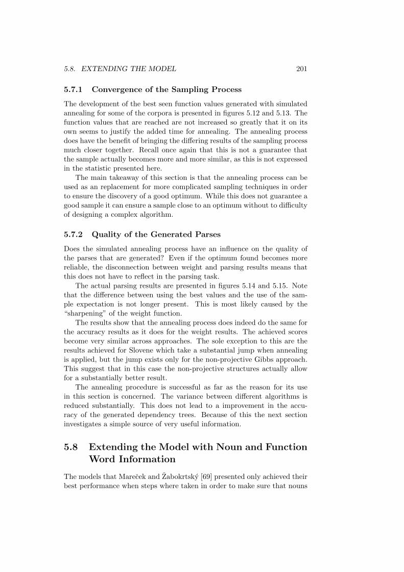
5.8. EXTENDING THE MODEL 201
5.7.1 Convergence of the Sampling Process
The development of the best seen function values generated with simulatedannealing for some of the corpora is presented in figures 5.12 and 5.13. Thefunction values that are reached are not increased so greatly that it on itsown seems to justify the added time for annealing. The annealing processdoes have the benefit of bringing the differing results of the sampling processmuch closer together. Recall once again that this is not a guarantee thatthe sample actually becomes more and more similar, as this is not expressedin the statistic presented here.
The main takeaway of this section is that the annealing process can beused as an replacement for more complicated sampling techniques in orderto ensure the discovery of a good optimum. While this does not guarantee agood sample it can ensure a sample close to an optimum without to difficultyof designing a complex algorithm.
5.7.2 Quality of the Generated Parses
Does the simulated annealing process have an influence on the quality ofthe parses that are generated? Even if the optimum found becomes morereliable, the disconnection between weight and parsing results means thatthis does not have to reflect in the parsing task.
The actual parsing results are presented in figures 5.14 and 5.15. Notethat the difference between using the best values and the use of the sam-ple expectation is not longer present. This is most likely caused by the“sharpening” of the weight function.
The results show that the annealing process does indeed do the same forthe accuracy results as it does for the weight results. The achieved scoresbecome very similar across approaches. The sole exception to this are theresults achieved for Slovene which take a substantial jump when annealingis applied, but the jump exists only for the non-projective Gibbs approach.This suggest that in this case the non-projective structures actually allowfor a substantially better result.
The annealing procedure is successful as far as the reason for its usein this section is concerned. The variance between different algorithms isreduced substantially. This does not lead to a improvement in the accu-racy of the generated dependency trees. Because of this the next sectioninvestigates a simple source of very useful information.
5.8 Extending the Model with Noun and FunctionWord Information
The models that Marecek and Zabokrtsky [69] presented only achieved theirbest performance when steps where taken in order to make sure that nouns
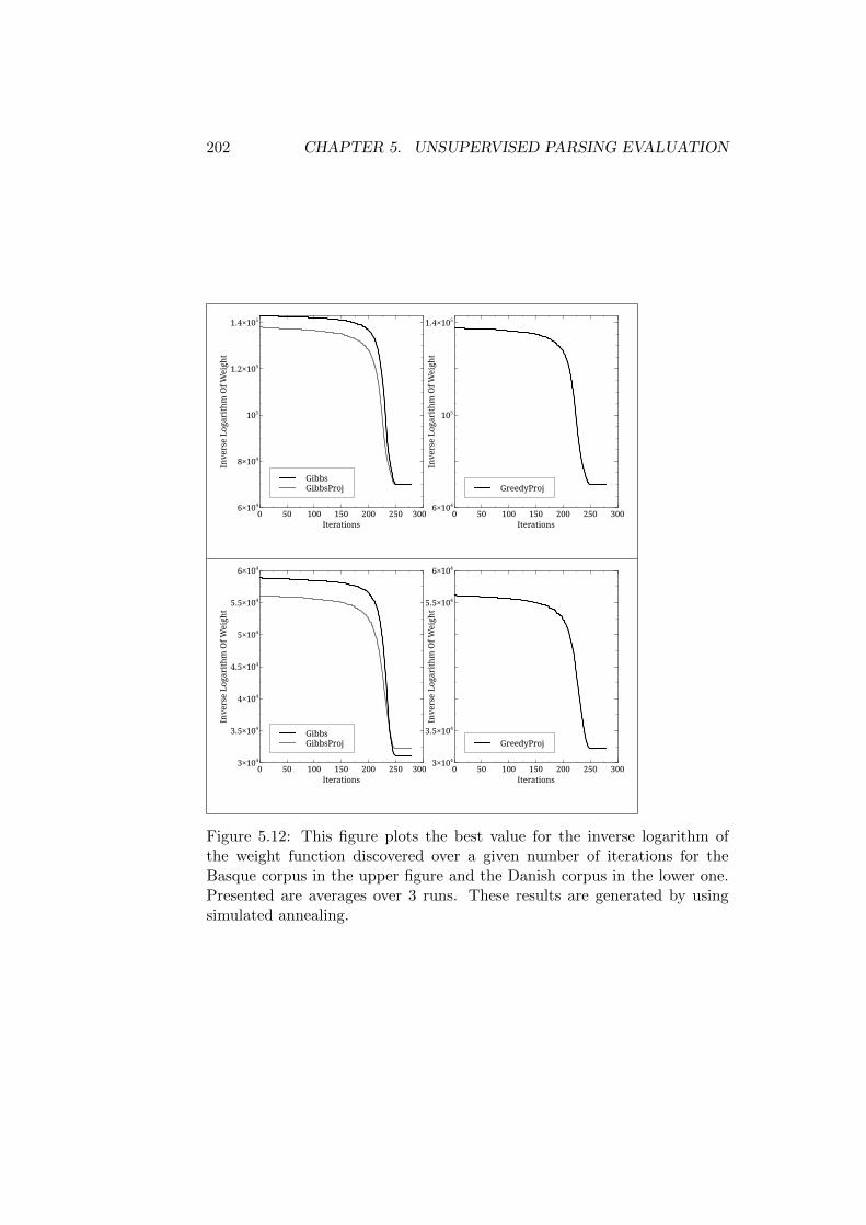
202 CHAPTER 5. UNSUPERVISED PARSING EVALUATION
GibbsGibbsProj
Inve
rse
Loga
rith
m O
f Wei
ght
6×10⁴
8×10⁴
105
1.2×10⁵
1.4×10⁵
Iterations0 50 100 150 200 250 300
GreedyProj
Inve
rse
Loga
rith
m O
f Wei
ght
6×10⁴
105
1.4×10⁵
Iterations0 50 100 150 200 250 300
GibbsGibbsProj
Inve
rse
Loga
rith
m O
f Wei
ght
3×10⁴
3.5×10⁴
4×10⁴
4.5×10⁴
5×10⁴
5.5×10⁴
6×10⁴
Iterations0 50 100 150 200 250 300
GreedyProj
Inve
rse
Loga
rith
m O
f Wei
ght
3×10⁴
3.5×10⁴
5.5×10⁴
6×10⁴
Iterations0 50 100 150 200 250 300
Figure 5.12: This figure plots the best value for the inverse logarithm ofthe weight function discovered over a given number of iterations for theBasque corpus in the upper figure and the Danish corpus in the lower one.Presented are averages over 3 runs. These results are generated by usingsimulated annealing.

5.8. EXTENDING THE MODEL 203
GibbsGibbsProj
Inve
rse
Loga
rith
m O
f Wei
ght
105
1.25×10⁵
1.5×10⁵
1.75×10⁵
2×10⁵
Iterations0 50 100 150 200 250 300
GreedyProj
Inve
rse
Loga
rith
m O
f Wei
ght
105
2×10⁵
Iterations0 50 100 150 200 250 300
GibbsGibbsProj
Inve
rse
Loga
rith
m O
f Wei
ght
6×10⁵
8×10⁵
106
1.2×10⁶
1.4×10⁶
Iterations0 50 100 150 200 250 300
GreedyProj
Inve
rse
Loga
rith
m O
f Wei
ght
6×10⁵
106
1.4×10⁶
Iterations0 50 100 150 200 250 300
Figure 5.13: This figure plots the best value for the inverse logarithm ofthe weight function discovered over a given number of iterations for theDutch corpus in the upper figure and the English corpus in the lower one.Presented are averages over 3 runs. These results are generated by usingsimulated annealing.
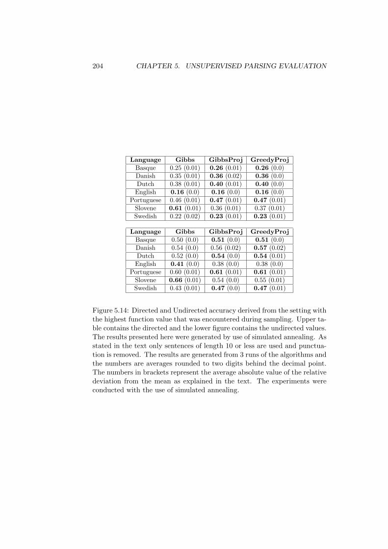
204 CHAPTER 5. UNSUPERVISED PARSING EVALUATION
Language Gibbs GibbsProj GreedyProjBasque 0.25 (0.01) 0.26 (0.01) 0.26 (0.0)Danish 0.35 (0.01) 0.36 (0.02) 0.36 (0.0)Dutch 0.38 (0.01) 0.40 (0.01) 0.40 (0.0)
English 0.16 (0.0) 0.16 (0.0) 0.16 (0.0)Portuguese 0.46 (0.01) 0.47 (0.01) 0.47 (0.01)
Slovene 0.61 (0.01) 0.36 (0.01) 0.37 (0.01)Swedish 0.22 (0.02) 0.23 (0.01) 0.23 (0.01)
Language Gibbs GibbsProj GreedyProjBasque 0.50 (0.0) 0.51 (0.0) 0.51 (0.0)Danish 0.54 (0.0) 0.56 (0.02) 0.57 (0.02)Dutch 0.52 (0.0) 0.54 (0.0) 0.54 (0.01)
English 0.41 (0.0) 0.38 (0.0) 0.38 (0.0)Portuguese 0.60 (0.01) 0.61 (0.01) 0.61 (0.01)
Slovene 0.66 (0.01) 0.54 (0.0) 0.55 (0.01)Swedish 0.43 (0.01) 0.47 (0.0) 0.47 (0.01)
Figure 5.14: Directed and Undirected accuracy derived from the setting withthe highest function value that was encountered during sampling. Upper ta-ble contains the directed and the lower figure contains the undirected values.The results presented here were generated by use of simulated annealing. Asstated in the text only sentences of length 10 or less are used and punctua-tion is removed. The results are generated from 3 runs of the algorithms andthe numbers are averages rounded to two digits behind the decimal point.The numbers in brackets represent the average absolute value of the relativedeviation from the mean as explained in the text. The experiments wereconducted with the use of simulated annealing.
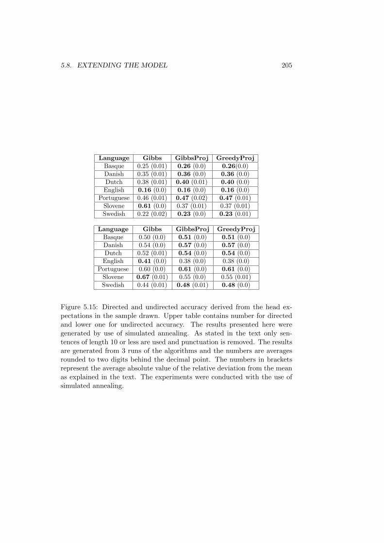
5.8. EXTENDING THE MODEL 205
Language Gibbs GibbsProj GreedyProjBasque 0.25 (0.01) 0.26 (0.0) 0.26(0.0)Danish 0.35 (0.01) 0.36 (0.0) 0.36 (0.0)Dutch 0.38 (0.01) 0.40 (0.01) 0.40 (0.0)
English 0.16 (0.0) 0.16 (0.0) 0.16 (0.0)Portuguese 0.46 (0.01) 0.47 (0.02) 0.47 (0.01)
Slovene 0.61 (0.0) 0.37 (0.01) 0.37 (0.01)Swedish 0.22 (0.02) 0.23 (0.0) 0.23 (0.01)
Language Gibbs GibbsProj GreedyProjBasque 0.50 (0.0) 0.51 (0.0) 0.51 (0.0)Danish 0.54 (0.0) 0.57 (0.0) 0.57 (0.0)Dutch 0.52 (0.01) 0.54 (0.0) 0.54 (0.0)
English 0.41 (0.0) 0.38 (0.0) 0.38 (0.0)Portuguese 0.60 (0.0) 0.61 (0.0) 0.61 (0.0)
Slovene 0.67 (0.01) 0.55 (0.0) 0.55 (0.01)Swedish 0.44 (0.01) 0.48 (0.01) 0.48 (0.0)
Figure 5.15: Directed and undirected accuracy derived from the head ex-pectations in the sample drawn. Upper table contains number for directedand lower one for undirected accuracy. The results presented here weregenerated by use of simulated annealing. As stated in the text only sen-tences of length 10 or less are used and punctuation is removed. The resultsare generated from 3 runs of the algorithms and the numbers are averagesrounded to two digits behind the decimal point. The numbers in bracketsrepresent the average absolute value of the relative deviation from the meanas explained in the text. The experiments were conducted with the use ofsimulated annealing.
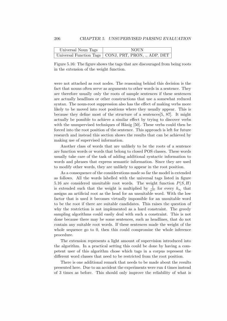
206 CHAPTER 5. UNSUPERVISED PARSING EVALUATION
Universal Noun Tags NOUN
Universal Function Tags CONJ, PRT, PRON, ., ADP, DET
Figure 5.16: The figure shows the tags that are discouraged from being rootsin the extension of the weight function.
were not attached as root nodes. The reasoning behind this decision is thefact that nouns often serve as arguments to other words in a sentence. Theyare therefore usually only the roots of sample sentences if these sentencesare actually headlines or other constructions that use a somewhat reducedsyntax. The noun-root suppression also has the effect of making verbs morelikely to be moved into root positions where they usually appear. This isbecause they define most of the structure of a sentences[5, 87]. It mightactually be possible to achieve a similar effect by trying to discover verbswith the unsupervised techniques of Hanig [50]. These verbs could then beforced into the root position of the sentence. This approach is left for futureresearch and instead this section shows the results that can be achieved bymaking use of supervised information.
Another class of words that are unlikely to be the roots of a sentenceare function words or words that belong to closed POS classes. These wordsusually take care of the task of adding additional syntactic information towords and phrases that express semantic information. Since they are usedto modify other words, they are unlikely to appear in the root position.
As a consequence of the considerations made so far the model is extendedas follows. All the words labelled with the universal tags listed in figure5.16 are considered unsuitable root words. The weight function P (S,H)is extended such that the weight is multiplied by 1
e25for every hsi that
assigns an artificial root as the head for an unsuitable word. With the lowfactor that is used it becomes virtually impossible for an unsuitable wordto be the root if there are suitable candidates. This raises the question ofwhy the restriction is not implemented as a hard constraint. The greedysampling algorithms could easily deal with such a constraint. This is notdone because there may be some sentences, such as headlines, that do notcontain any suitable root words. If these sentences made the weight of thewhole sequence go to 0, then this could compromise the whole inferenceprocedure.
The extension represents a light amount of supervision introduced intothe algorithm. In a practical setting this could be done by having a com-petent user of this algorithm chose which tags in a corpus represent thedifferent word classes that need to be restricted from the root position.
There is one additional remark that needs to be made about the resultspresented here. Due to an accident the experiments were run 4 times insteadof 3 times as before. This should only improve the reliability of what is
5.8. EXTENDING THE MODEL 207
presented. It is however necessary to explain this difference to the otherexperiments. For the experiments annealing is once again used in order tomake everything more stable.
5.8.1 Convergence of the Sampling Process
A small set of evaluations of the best result seen up to a iteration is presentedin figure 5.17. The characteristic “sharp dip” that the best seen functionvalue showed in all previous experiments still occurs much later than it didwhen no annealing was used, but it comes much earlier than it did withannealing before. This is most likely because the force towards a certainroot guides the induction process and therefore induction is less dependenton the other assignments made so far.
The weights reached are not substantially worse than those that arereached with annealing in the case of the original model. The difference isstill large enough to suggest that some sentences cannot be parsed withoutassigning an unsuitable word to the root position.
5.8.2 Quality of the Generated Parses
Figures 5.18 and 5.19 contain the accuracy numbers that are achieved withthe additional suppression of noun and function word roots. There is a largeimprovement. The numbers are still not high enough to compare to the stateof the art values. At the same time the numbers show that it is possible toachieve good performance with the sampling algorithms when the model isspecified correctly.
It could be argued that the improvement in performance is due to thegreater ease of convergence since part of the model, namely the factors addedfor suppression of certain roots, do not change with different assignments.This is in contrast to the the remainder of the model that is dependent oncounts of observations that constantly change as assignments change. Thisargumentation would not stick since the results presented earlier stronglysuggest that the sampling process does not make any large changes by thetime it ends.
It should be noted that there is once again a difference between theresults generated by sampling and those that come from the use of the bestseen value. The difference is no longer purely in favour of the sampling basedapproach and it is once again a relatively small effect. One would expectthat the weight function becomes more focused on a single point if certainroots are ruled out and that the difference between the best function and theexpected values would actually become smaller with the added constraint.It would be a topic for further investigation what causes this behaviour.
The projective algorithms perform better than the non-projective oneswith the root constraint for all languages other than Basque. It seems
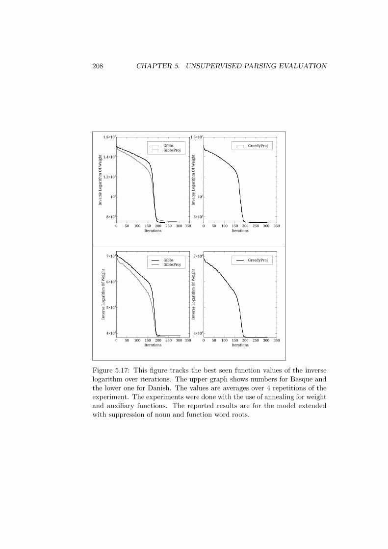
208 CHAPTER 5. UNSUPERVISED PARSING EVALUATION
GibbsGibbsProj
Inve
rse
Loga
rith
m O
f Wei
ght
8×10⁴
105
1.2×10⁵
1.4×10⁵
1.6×10⁵
Iterations0 50 100 150 200 250 300 350
GreedyProj
Inve
rse
Loga
rith
m O
f Wei
ght
8×10⁴
105
1.6×10⁵
Iterations0 50 100 150 200 250 300 350
GibbsGibbsProj
Inve
rse
Loga
rith
m O
f Wei
ght
4×10⁴
5×10⁴
6×10⁴
7×10⁴
Iterations0 50 100 150 200 250 300 350
GreedyProj
Inve
rse
Loga
rith
m O
f Wei
ght
4×10⁴
7×10⁴
Iterations0 50 100 150 200 250 300 350
Figure 5.17: This figure tracks the best seen function values of the inverselogarithm over iterations. The upper graph shows numbers for Basque andthe lower one for Danish. The values are averages over 4 repetitions of theexperiment. The experiments were done with the use of annealing for weightand auxiliary functions. The reported results are for the model extendedwith suppression of noun and function word roots.
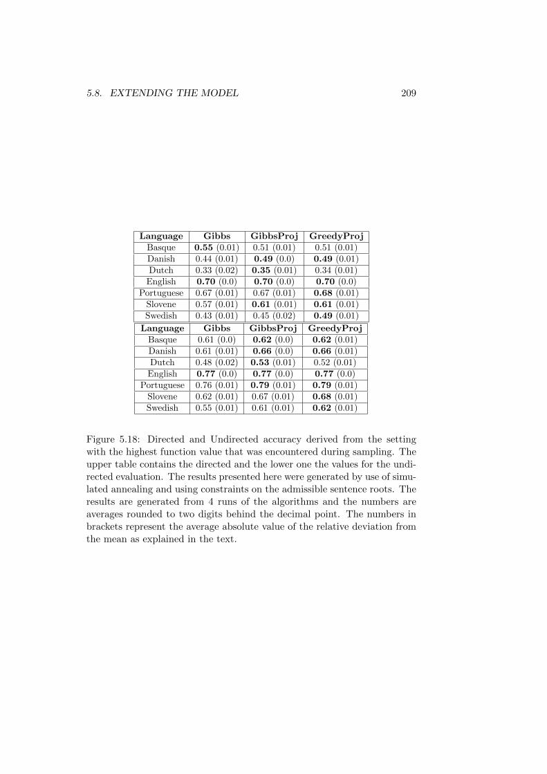
5.8. EXTENDING THE MODEL 209
Language Gibbs GibbsProj GreedyProjBasque 0.55 (0.01) 0.51 (0.01) 0.51 (0.01)Danish 0.44 (0.01) 0.49 (0.0) 0.49 (0.01)Dutch 0.33 (0.02) 0.35 (0.01) 0.34 (0.01)
English 0.70 (0.0) 0.70 (0.0) 0.70 (0.0)Portuguese 0.67 (0.01) 0.67 (0.01) 0.68 (0.01)
Slovene 0.57 (0.01) 0.61 (0.01) 0.61 (0.01)Swedish 0.43 (0.01) 0.45 (0.02) 0.49 (0.01)
Language Gibbs GibbsProj GreedyProjBasque 0.61 (0.0) 0.62 (0.0) 0.62 (0.01)Danish 0.61 (0.01) 0.66 (0.0) 0.66 (0.01)Dutch 0.48 (0.02) 0.53 (0.01) 0.52 (0.01)
English 0.77 (0.0) 0.77 (0.0) 0.77 (0.0)Portuguese 0.76 (0.01) 0.79 (0.01) 0.79 (0.01)
Slovene 0.62 (0.01) 0.67 (0.01) 0.68 (0.01)Swedish 0.55 (0.01) 0.61 (0.01) 0.62 (0.01)
Figure 5.18: Directed and Undirected accuracy derived from the settingwith the highest function value that was encountered during sampling. Theupper table contains the directed and the lower one the values for the undi-rected evaluation. The results presented here were generated by use of simu-lated annealing and using constraints on the admissible sentence roots. Theresults are generated from 4 runs of the algorithms and the numbers areaverages rounded to two digits behind the decimal point. The numbers inbrackets represent the average absolute value of the relative deviation fromthe mean as explained in the text.
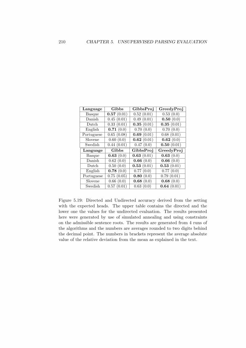
210 CHAPTER 5. UNSUPERVISED PARSING EVALUATION
Language Gibbs GibbsProj GreedyProjBasque 0.57 (0.01) 0.52 (0.01) 0.53 (0.0)Danish 0.45 (0.01) 0.49 (0.01) 0.50 (0.0)Dutch 0.33 (0.01) 0.35 (0.01) 0.35 (0.01)
English 0.71 (0.0) 0.70 (0.0) 0.70 (0.0)Portuguese 0.65 (0.08) 0.69 (0.01) 0.68 (0.01)
Slovene 0.60 (0.0) 0.62 (0.01) 0.62 (0.0)Swedish 0.44 (0.01) 0.47 (0.0) 0.50 (0.01)
Language Gibbs GibbsProj GreedyProjBasque 0.63 (0.0) 0.63 (0.01) 0.63 (0.0)Danish 0.62 (0.0) 0.66 (0.0) 0.66 (0.0)Dutch 0.50 (0.0) 0.53 (0.01) 0.53 (0.01)
English 0.78 (0.0) 0.77 (0.0) 0.77 (0.0)Portuguese 0.75 (0.05) 0.80 (0.0) 0.79 (0.01)
Slovene 0.66 (0.0) 0.68 (0.0) 0.68 (0.0)Swedish 0.57 (0.01) 0.63 (0.0) 0.64 (0.01)
Figure 5.19: Directed and Undirected accuracy derived from the settingwith the expected heads. The upper table contains the directed and thelower one the values for the undirected evaluation. The results presentedhere were generated by use of simulated annealing and using constraintson the admissible sentence roots. The results are generated from 4 runs ofthe algorithms and the numbers are averages rounded to two digits behindthe decimal point. The numbers in brackets represent the average absolutevalue of the relative deviation from the mean as explained in the text.
5.9. CONCLUSION AND FURTHER RESEARCH 211
that with a little more linguistic information it is possible for the projectiveconstraint to make at least a small positive contribution.
The main takeaway of this sections is the fact that the MCMC techniquecan be used in the weakly supervised learning of dependency trees. In con-trast to approaches like that of Naseem et. al. [80], which use very concreterules to improve parsing results, the constraint presented here is very vagueand does not contain much information about which words are supposed tobe in which relations.
5.9 Conclusion and Further Research
This chapter has combined both positive and negative results for the differ-ent sampling algorithms. The positive results are represented by the factthat the algorithms can reliably and predictably find optima of a weight func-tion that creates complicated relationships between the different dependencyassignments made for a whole corpus of sentences, the good performance ofthe GreedyProj algorithm and relatively good parses that result when themodel is modified in order to prevent noun and function word roots. Thefirst negative is the low accuracy numbers produced with the base model.While the sampling process finds trees that do well in terms of the definedmodel, it seems that a better value does not correspond to better parsing.The second negative result is the fact that, at least without annealing, therecan be large differences in the performance of the sampling algorithms. Alast negative result is the weaker performance of the algorithms that onlyhave the greedy sampling step to find a good root word. This problem isnot present in the GreedyProj algorithm. This suggest that the other algo-rithms could perform as well as this algorithm if they were combined withthe root picking step used in the Gibbs algorithms to give an example.
The main takeaways of this section are as follows:
• Annealing can be used to reliably find a good result and reduce thedifferences between algorithms.
• If only a quick and possibly suboptimal solution is needed, then theMH and MHProj algorithms can be used.
• At least for the task of local optimization Gibbs can be used. It quicklydiscovers a good setting of the assignments and does this for all thecorpora in the set.
• In the model used here the projective constraint does not contributemuch to a more accurate solution. The constraint does not preventtechniques from working towards a solution quickly. Eventual differ-ences between GibbsProj and Gibbs can be removed by annealing.

212 CHAPTER 5. UNSUPERVISED PARSING EVALUATION
• The combined algorithm GreedyProj can be used to optimize the tar-get function very well. It may also be able to generate a good samplefrom the function.
• The use of expected heads instead of the best assignment leads toslightly better results than using only the best assignment. The differ-ence is too slight to justify the use of sampling on its own. Since thissection serves mainly to investigate the performance of the algorithms,it is still a result of interest.
• The edge factored global sampling step does not add much perfor-mance over the head by head approach with which it is combined.
Overall the results presented in this chapter are not as encouraging asthose from chapter 4. Everything presented here can still be used to comeup with some guidelines on the use of the sampling algorithms. The opti-mization of the weight function is only an auxiliary measure for the qualityof the sampling process, but the Gibbs algorithms did well on this task inthis section. The algorithm reaches its final value quickly and if this is theonly goal then the algorithm can be used without any auxiliary function.
Chapter 6
Conclusion and FurtherResearch
This chapter gives a short summary of the thesis. The main objective ofthis is to pronounce the gain in knowledge achieved. From this analysis it isalso possible to derive some possible directions of future research that couldbe undertaken in order to extend and sharpen what was observed here.
The main takeaways of the investigation made here are of course the algo-rithms that have been presented. This is not restricted to simply presentingthe algorithms. Along with them came proves of their correctness and, mostimportantly, a thorough investigation of the behaviour of the algorithms ontwo inference problems. The artificial problem that was presented in chap-ter 4 helped investigate the actual convergence of the sampling algorithmstowards correct expectations. The more applied problem that was discussedin chapter 5 could not be investigated for correctness against any predictablestatistic. What could be drawn from the research made in that chapter isthe fact that the sampling process quickly moves towards some high proba-bility area in which the MCMC algorithm then moves in order to generate adraw from the desired distribution. Since MCMC algorithms generally onlyrequire the computation of ratios between weight functions, the results alsosuggest that the algorithms presented here could be used as simple defaultalgorithms to implement optimization during the development of algorithmsthat deal with dependency structures.
The following sections first review the results of the thesis in section 6.1.There is no one simple conclusion that can be drawn from the experimentsmade here. Therefore these results are split up into multiple points in orderto elaborate on the different aspects that need to be highlighted.
After a review of the thesis section 6.2 discusses what could be done withthe discoveries made here. The testing of the different sampling algorithmscould obviously be extended arbitrarily. Beside this obvious direction forfuture research a short mention is made of other techniques that could be
213
214 CHAPTER 6. CONCLUSION AND FURTHER RESEARCH
used with the MCMC algorithms developed here.
6.1 Results
The primary result of the the thesis is a toolbox of different MCMC samplingalgorithms for dependency trees. The algorithms developed here came in twoflavours. The first where algorithms that sample head assignments one at atime. This can be costly if the Gibbs approach is used and it is necessary toevaluate all possible settings for every word in a sampling step. It may bepossible to make this more efficient if it is possible to drop a number of termsin the computation of weights that are needed. This is an optimization thatis specific to every model for which the samplers are to be used. Thereforethis optimization was not discussed here.
One of the results in this thesis that is not one of the main foci of thissummary is the performance of the unsupervised learning model presentedin chapter 5. The model is a slightly extended version of the one presentedby Marecek and Zabokrtsky [69]. The only extension is the addition of afertility model. It seems that the model alone is not able to determine gooddependency trees. Taking another hint from Marecek and Zabokrtsky [69]the concept of unsuitable roots is added to the model and this can be usedto show that the poor performance is not a result of the sampling algorithmsbut rather caused by a poor modelling of dependency relations.
The MCMC schemes presented here have shown different strengths andweaknesses and it is therefore necessary to make a subdivided presentationof the different conclusions that can be drawn from the thesis. This is donein the rest of the section.
6.1.1 The Surprising Helpfulness of Restricted Options
One of the things this thesis set out to show is that it is possible to sam-ple subsets of the full set of dependency structures. The first step in thiswas giving a set of simple algorithms that can compute the possible headsfor a word given the other edges in the sentence. Then it was shown that,with the use of this simple algorithms, it is possible to sample the set ofdependency trees, both projective and non-projective correctly. Another re-striction to the set of trees that was discussed is limiting the investigationto a single root. This required some additional techniques that are inter-esting in themselves, since linguistic structures will often have one or fewroot nodes. Another reason why this constraint is interesting is the fact thatmost of these techniques could be re-purposed in order to deal with similarconstraints like demanding that a certain word may have at most one childor that words have one of a certain set of argument frames.
Investigation on the different tasks showed that there are actual benefitsto the convergence and optimization side of sampling that can result from
6.1. RESULTS 215
restricting the set of possible trees and then moving exclusively on this set.In the artificial evaluation task the projective samplers showed a greaterrobustness than the sampling algorithms that visited all possible trees. Itis possible that this improvement is partly the result of a reduction in apossible bias. There is an additional benefit in using only projective trees asfar as performance goes. The algorithm that was used to find projective headcandidates is asymptotically no more costly than those used to compute non-projective head candidates. Therefore the amount of additional time spentreducing the head candidates in order to ensure projective trees can easilybe made up for by a smaller number of function evaluations needed in theGibbs inspired and greedy algorithms.
The projective greedy sampler proved to be the best in the task of func-tion optimization on the unsupervised task and in the artificial problemshowed the ability to handle a very complex sampling problem. The pro-jective Gibbs sampler is less reliable for optimization but performed muchbetter than the non-projective version in the artificial task. The same canbe said for the sampler based on uniform selection. The strength of samplersfor restricted options is an interesting and important takeaway and it maybe possible to investigate even more restrictions in the future. It would beimportant that these added restrictions are also linguistically motivated sothat they do not rule out any choices that would be necessary for the use ofthe dependency samplers in Natural Language Processing.
6.1.2 Usefulness of Global Steps
The thesis showed that with a good approximation of the actual weightfunction it is possible to implement a change of the complete structure ina single sampling step. This can be exceptionally helpful when complexweight functions are sampled or when there are sharp local optima. At thesame time this opens the possibility of a bad design of the auxiliary function.In this thesis this problem was highlighted when the greedy step was notable to select a correct root of a sentence in the unsupervised task. Oneway it was attempted to handle this problem was by combining the globalsampling steps with the global steps.
Even the relatively simple edge factored approximation helped substan-tially with the handling of the artificial inference task. The influence is notnoticeable in the unsupervised task in which the Gibbs steps can easily doall of the heavy lifting necessary.
The general takeaway would be that it is possible to achieve a lot with theuse of global steps if it is possible to design a appropriate auxiliary functionand the function to be sampled from is actually complicated enough tojustify the use of such a complicated tool.
216 CHAPTER 6. CONCLUSION AND FURTHER RESEARCH
6.1.3 The Surprising Efficiency of Simple Samplers
The simple head by head sampling algorithms can be be thrown off by using atarget function that introduces very complex relations between the differenthead assignments. This was shown by the artificial sampling problem. Itis possible to somewhat reduces this problem by using more than one chainrun in parallel, but it will become a more pronounced problem when thenumber of relevant optima of the target function increases. The simplesampling algorithms can usually guarantee a substantial improvement inthe weight of the sampled structures even if they cannot move between theoptima.
The most well known global approach in sampling for Natural LanguageProcessing is the algorithm for sampling binary trees introduced by Chapel-lier and Rajman [17] and applied to corpus wide inference through MCMCby Johnson et. al. [56]. Like the algorithms presented here these globalapproaches will generally need the possibility to approximate the weightfunction. Designing this function is something that can easily be avoidedwhen the simple head by head algorithms are used. Then it is only necessaryto be able to evaluate the weight function somewhat efficiently. This makesthe simple algorithms an interesting out of the box solution that can be usedin the design of future models and tasks.
6.1.4 The Reliability of Gibbs Sampling
One goal that this thesis set out to achieve was to show that Gibbs sampling,which was used to a small extend in previous research on dependency trees,can be applied to a broad set of dependency sampling tasks without havingto do much additional design of algorithms and without having to wastefullyoperate on the set of all dependency trees and then restrict the sampled setafterwards.
One design that had to be contributed was a possibility for the Gibbsalgorithms to sample single attachments, specifically single roots. This tech-nique is similar in style to the general Gibbs approach and leads to a pleas-antly simple rule of rejecting new roots based on the ratio of the trees pos-sible with the old and the new root. With this tool and the computation ofthe possible head candidates it is possible to apply the simple Gibbs samplerwidely and reliably. It is not necessary to develop a clever re- parametriza-tion of the problem to allow for the use of Gibbs sampling [67]. When oneis ready to pay the price of additional weight function evaluations, then theGibbs algorithm will at the very least quickly find a solution with a weightcomparable to that found by other algorithms.
6.2. FURTHER RESEARCH 217
6.2 Further Research
In this section some future research directions that additional investigationcould be directed towards are presented. It is typical of nearly any researchthat it raises about as much questions as it answers, if not more. This isof course also the case for this thesis. Even with this admission there arestill some clear future directions of research that open up. One of the mostobvious ones are open problems from this thesis such as:
• If there are widely applicable way of designing the auxiliary functionsfor edge factored and greedy sampling that can make it less difficultto use these algorithms.
• In this thesis the evaluation was focused on single rooted trees. Thiswas done in order to be able to evaluate all aspects of the algorithmsdeveloped here. It was also done to limit the size of the thesis. It wouldeasily be possible to switch out different root sampling approaches foreach other.
• Can the seeming initial bias of the Gibbs algorithms be reduced byrandomizing the order in which head assignments are sampled and inwhich root nodes are proposed.
These and additional extension questions were already mentioned in themain text of the thesis. In the following few sections some extensions arementioned that are not direct consequences of the things discussed in thethesis. They represent combinations of the results presented here with someadditional research presented in other texts.
6.2.1 Other Unsupervised Dependency Models
As already mentioned in the text it was researched in preliminary investi-gations whether the sampler could be successfully combined with the DMVmodel by Klein and Manning [57]. These investigations, which were notpresented here, could not produce any results that are better than what wasshown. This could be due to the sampling algorithm moving away from anyclever initialization that is necessary or some other reason. In the future itcould be attempted to combine the DMV with the alignment inspired modelthat was used here.
The alignment based model does not include any information on whethera words should have children on one or the other of its sides. It also doesnot model any connection between the numbers of children, or among thedifferent distances. If a word tends to be right next to its head, then thisdoes not mean that it becomes more likely for it to appear in a distance ofone word any more than it becomes more likely to be in distance ten. Thiscould be remedied in extended models.

218 CHAPTER 6. CONCLUSION AND FURTHER RESEARCH
It was very helpful to add linguistic knowledge to the model of depen-dency trees. This was done by suppressing unsuitable dependency roots. Infuture research it would be possible to decide which words are suitable orunsuitable as roots in an unsupervised fashion such as the verb detectionapproach by Hanig [50] or the function content word separation presentedby Zhao and Marcus [121].
The bad performance of the unsupervised inference is one of the mainweak points of what was presented. There is still a great amount of headwaythat could be made in this direction.
6.2.2 Use with Different Tasks
There is only a limited amount of space that can be used for any investigationin a single thesis. This meant that the results that could be presented herewere limited to one artificial task and one more applied topic. It would beof great interest to know what results can be drawn from evaluations withadditional tasks.
One possible additional topic of investigation is the use of the computa-tion of expectations in order to train models similar to conditional randomfields[35, 60]. If it is possible to approximate feature counts, then one couldtrain models based on global properties of a dependency tree.
The samplers could also be extended to include a mapping from depen-dency structures to sentences in order to use the samplers in tasks such asmachine translation. This has already been done for the sampling of parsetrees [29, 120] and it would be interesting if dependency trees can be suc-cessful in complex translation models if sampling is used to compute theexpected translations for a sentence.
6.2.3 Population Based Techniques
In recent years there has been a move to combine techniques such as geneticalgorithms with sampling approaches in order to improve both [10, 64, 62].Since the research here has had the implication that it can be helpful touse a number of parallel chains, this would be of great interest in futureinvestigations. If parallel chains are run in order to improve convergence, itmay be helpful to add such population based techniques to further help thesampling process.
There are also other approaches such as Population Monte Carlo [15, 55]that are not instances of Markov Chain Monte Carlo techniques, but makeuse of similar transitions. It would be possible to combine the algorithmspresented here with those techniques. The question is then whether thiswould improve the performance of the sampling approach that results or ifthe required population size is to great for a successful application.

6.3. CONCLUSION 219
6.3 Conclusion
This section reviewed some of the results of this thesis. It also suggestedsome future research directions. As stated before this thesis introduced asmany new questions as it answered. It did have some relevant takeawayshowever. A set of tools for dependency sampling being the most importantone. The ideas presented here could be applied to a number of new problemsand enable a large amount of follow-up research.

220 CHAPTER 6. CONCLUSION AND FURTHER RESEARCH

Chapter 7
Bibliography
[1] Ajith Abraham, He Guo, and Hongbo Liu. Swarm intelligence: Foun-dations, perspectives and applications. In Nadia Nedjah and Luizade Macedo Mourelle, editors, Swarm Intelligent Systems, volume 26of Studies in Computational Intelligence, pages 3–25. Springer, 2006.
[2] Ethem Alpaydin. Introduction to Machine Learning (Adaptive Com-putation and Machine Learning). The MIT Press, 2004.
[3] David Barber. Bayesian Reasoning and Machine Learning. CambridgeUniversity Press, 2012.
[4] Leonard E. Baum, Ted Petrie, George Soules, and Norman Weiss. Amaximization technique occurring in the statistical analysis of proba-bilistic functions of markov chains. The Annals of Mathematical Statis-tics, 41(1):164–171, 1970.
[5] Emily M. Bender. Linguistic Fundamentals for Natural Language Pro-cessing: 100 Essentials from Morphology And Syntax. Morgan & Clay-pool Publishers, 2013.
[6] Christopher M. Bishop. Pattern Recognition and Machine Learning(Information Science and Statistics). Springer-Verlag New York, Inc.,Secaucus, NJ, USA, 2006.
[7] Yonatan Bisk and Julia Hockenmaier. Induction of linguistic structurewith combinatory categorial grammars. In Proceedings of the NAACL-HLT 2012 Workshop on Inducing Linguistic Structure Shared Task,pages 90–95, 2012.
[8] Phil Blunsom and Trevor Cohn. Unsupervised induction of tree sub-stitution grammars for dependency parsing. In Proceedings of the 2010Conference on Empirical Methods in Natural Language Processing,pages 1204–1213. Association for Computational Linguistics, 2010.
221
222 CHAPTER 7. BIBLIOGRAPHY
[9] Rens Bod, Remko Scha, and Khalil Sima’an, editors. Data OrientedParsing. Center for the Study of Language and Information, Stanford,California, 2003.
[10] Cajo J. F. Ter Braak. Genetic algorithms and markov chain montecarlo: Differential evolution markov chain makes bayesian computingeasy. Technical report, Biometris, Wageningen University and Re-search Centre, Wageningen, The Netherlands, 2004.
[11] Andrei Broder. Generating random spanning trees. In Proceedingsof the 30th Annual Symposium on Foundations of Computer Science,pages 442–447. IEEE Computer Society, 1989.
[12] Samuel Brody. It depends on the translation: unsupervised depen-dency parsing via word alignment. In Proceedings of the 2010 Con-ference on Empirical Methods in Natural Language Processing, pages1214–1222, 2010.
[13] Peter F. Brown, Vincent J. Della Pietra, Stephen A. Della Pietra,and Robert L. Mercer. The mathematics of statistical machine trans-lation: parameter estimation. Computational Linguistics, 19(2):263–311, June 1993.
[14] Olivier Cappe, Simon J. Godsill, and Eric Moulines. An overview ofexisting methods and recent advances in sequential monte carlo. InProceedings of the IEEE, 2007.
[15] Olivier Cappe, Arnaud Guillin, Jean-Michel Marin, and ChristianRobert. Population monte carlo. Journal of Computational andGraphical Statistics, 13(4):907–929, 2004.
[16] Nathanael Chambers and Dan Jurafsky. Template-based informationextraction without the templates. In Proceedings of the 49th AnnualMeeting of the Association for Computational Linguistics: HumanLanguage Technologies, pages 976–986. Association for ComputationalLinguistics, 2011.
[17] Jean-Cedric Chappelier and Martin Rajman. Monte-carlo sampling fornp-hard maximization problems in the framework of weighted parsing.In Natural Language Processing - NLP 2000, Second InternationalConference, volume 1835 of Lecture Notes in Computer Science, pages106–117. Springer, 2000.
[18] Eugene Charniak. The brain as a statistical inference engine - and youcan too. Computational Linguistics, 37(4):1 – 13, August 2011.
223
[19] David Chiang, Jonathan Graehl, Kevin Knight, Adam Pauls, and Su-jith Ravi. Bayesian inference for finite-state transducers. In HLT ’10:Human Language Technologies: The 2010 Annual Conference of theNorth American Chapter of the Association for Computational Lin-guistics, pages 447–455. Association for Computational Linguistics,2010.
[20] Tagyoung Chung, Licheng Fang, Daniel Gildea, and DanielStefankovic. Sampling tree fragments from forests. ComputationalLinguistics, 40(1), 2013.
[21] Shay B. Cohen, Dipanjan Das, and Noah A. Smith. Unsupervisedstructure prediction with non-parallel multilingual guidance. In Pro-ceedings of the 2011 Conference on Empirical Methods in Natural Lan-guage Processing, pages 50–61. The Association for ComputationalLinguistics, 2011.
[22] Shay B. Cohen and Noah A. Smith. Covariance in unsupervised learn-ing of probabilistic grammars. Journal of Machine Learning Research,11:3017–3051, December 2010.
[23] Charles J. Colbourn, Wendy J. Myrvold, and Eugene Neufeld. Two al-gorithms for unranking arborescences. Journal of Algorithms, 20:268–281, 1996.
[24] Aron Culotta and Jeffrey Sorensen. Dependency tree kernels for re-lation extraction. In Proceedings of the 42nd Annual Meeting of theAssociation for Computational Linguistics, 2004.
[25] Sajib Dasgupta and Vincent Ng. Unsupervised part-of-speech acquisi-tion for resource-scarce languages. In EMNLP-CoNLL 2007, Proceed-ings of the 2007 Joint Conference on Empirical Methods in NaturalLanguage Processing and Computational Natural Language Learning,pages 218–227, 2007.
[26] Hal Daume III. Fast search for dirichlet process mixture models. InProceedings of the Eleventh International Conference on Artificial In-telligence and Statistics (AIStats), 2007.
[27] Hal Daume III, John Langford, and Daniel Marcu. Search-based struc-tured prediction. Machine Learning, 75:297–325, 2009.
[28] Arthur P. Dempster, Nan M. Laird, and Donald B. Rubin. Maximumlikelihood from incomplete data via the em algorithm. Journal of theRoyal Statistical Society. Series B (Methodological), 39(1):1–38, 1977.
224 CHAPTER 7. BIBLIOGRAPHY
[29] John DeNero, Alexandre Bouchard-Cote, and Dan Klein. Samplingalignment structure under a bayesian translation model. In Proceed-ings of the Conference on Empirical Methods in Natural Language Pro-cessing, EMNLP ’08, pages 314–323. Association for ComputationalLinguistics, 2008.
[30] Madalina M. Drugan and Dirk Thierens. Evolutionary markov chainmonte carlo. In Artificial Evolution, 6th International Conference,Evolution Artificielle, EA 2003, pages 63–76, 2003.
[31] Gregory Dubbin and Phil Blunsom. Unsupervised part of speech infer-ence with particle filters. In Proceedings of the NAACL-HLT Workshopon the Induction of Linguistic Structure, pages 47–54. Association forComputational Linguistics, 2012.
[32] Jason M. Eisner. Three new probabilistic models for dependency pars-ing: an exploration. In Proceedings of the 16th conference on Compu-tational linguistics - Volume 1, pages 340–345. Association for Com-putational Linguistics, 1996.
[33] Manaal Faruqui and Sebastian Pado. Training and evaluating a ger-man named entity recognizer with semantic generalization. In Pro-ceedings of KONVENS 2010, 2010.
[34] Jenny Rose Finkel, Trond Grenager, and Christopher Manning. Incor-porating non-local information into information extraction systems bygibbs sampling. In Proceedings of the 43rd Annual Meeting on Asso-ciation for Computational Linguistics, pages 363–370. Association forComputational Linguistics, 2005.
[35] Jenny Rose Finkel, Alex Kleeman, and Christopher D. Manning. Ef-ficient, feature-based, conditional random field parsing. In ACL 2008,Proceedings of the 46th Annual Meeting of the Association for Com-putational Linguistics, pages 959–967, 2008.
[36] Jenny Rose Finkel and Christopher D. Manning. Nested named en-tity recognition. In Proceedings of the 2009 Conference on EmpiricalMethods in Natural Language Processing, pages 141–150. Associationfor Computational Linguistics, 2009.
[37] David Flanagan. Java In A Nutshell. O’Reilly Media, 2005.
[38] Bela A. Frigyik, Amol Kapila, and Maya R. Gupta. Introductionto the dirichlet distribution and related processes. Technical report,University of Washington, 2010.
225
[39] Victoria A. Fromkin, Susan Curtiss, Bruce P. Hayes, Nina Hyams,Patricia A. Keating, Hilda Koopman, Pamela Munro, DominiqueSportiche, Edward P. Stabler, Donca Steriade, Tim Stowell, and AnnaSzabolcsi. Linguistics - An Introduction to Linguistic Theory. Black-well Publishing Ltd., 2000.
[40] Dani Gamerman and Hedibert F. Lopes. Markov Chain Monte Carlo -Stochastic Simulation for Bayesian Inference. Chapman & Hall/CRC,2006.
[41] Kuzman Ganchev, Joao Graca, Jennifer Gillenwater, and Ben Taskar.Posterior regularization for structured latent variable models. Journalof Machine Learning Research, 11:2001–2049, 2010.
[42] Jianfeng Gao, Jian-Yun Nie, Guangyuan Wu, and Guihong Cao. De-pendence language model for information retrieval. In Proceedings ofthe 27th annual international ACM SIGIR conference on Research anddevelopment in information retrieval, pages 170–177, 2004.
[43] Jianfeng Gao and Hisami Suzuki. Unsupervised learning of depen-dency structure for language modeling. In Proceedings of the 41st An-nual Meeting of the Association for Computational Linguistics, pages521–528, 2003.
[44] Carl Geiger and Christian Kanzow. Numerische Verfahren zur Losungunrestringierter Optimierungsaufgaben. Springer, 1999.
[45] Douwe Gelling, Trevor Cohn, Phil Blunsom, and Joao Graca. Thepascal challenge on grammar induction. In Proceedings of the NAACL-HLT Workshop on the Induction of Linguistic Structure, pages 64–80.Association for Computational Linguistics, 2012.
[46] Stuart Geman and Donald Geman. Stochastic relaxation, gibbs distri-butions, and the bayesian restoration of images. In Martin A. Fischlerand Oscar Firschein, editors, Readings in computer vision: issues,problems, principles, and paradigms, pages 564–584. Morgan Kauf-mann Publishers Inc., 1987.
[47] Kevin Gimpel, Nathan Schneider, Brendan O’Connor, Dipanjan Das,Daniel Mills, Jacob Eisenstein, Michael Heilman, Dani Yogatama, Jef-frey Flanigan, and Noah A. Smith. Part-of-speech tagging for twitter:Annotation, features, and experiments. In The 49th Annual Meetingof the Association for Computational Linguistics: Human LanguageTechnologies, Short Papers, pages 42–47, 2011.
[48] Joshua Goodman. Parsing algorithms and metrics. In Proceedings ofthe 34th annual meeting on Association for Computational Linguistics,pages 177–183. Association for Computational Linguistics, 1996.
226 CHAPTER 7. BIBLIOGRAPHY
[49] T. L. Griffiths, M. Steyvers, D. Blei, and J. B. Tenenbaum. Integrat-ing topics and syntax. Advances in Neural Information ProcessingSystems, 17:537–544, 2005.
[50] Christian Hanig. Knowledge-free verb detection through tag sequencealignment. In Proceedings of the 18th Nordic Conference of Computa-tional Linguistics. Association for Computational Linguistics, 2011.
[51] Nora Hartsfield and Gerhard Ringel. Pearls in Graph Theory: A Com-prehensive Introduction. Dover Publications, 2003.
[52] William P. Headden, III, Mark Johnson, and David McClosky. Im-proving unsupervised dependency parsing with richer contexts andsmoothing. In NAACL ’09: Proceedings of Human Language Tech-nologies: The 2009 Annual Conference of the North American Chap-ter of the Association for Computational Linguistics, pages 101–109.Association for Computational Linguistics, 2009.
[53] William P. Headden, III, David McClosky, and Eugene Charniak.Evaluating unsupervised part-of-speech tagging for grammar induc-tion. In COLING ’08: Proceedings of the 22nd International Con-ference on Computational Linguistics, pages 329–336. Association forComputational Linguistics, 2008.
[54] Hans Jurgen Heringer. Morphologie. Wilhelm Fink, 2009.
[55] Ajay Jasra, David A. Stephens, and Christopher C. Holmes. Onpopulation-based simulation for static inference. Statistics and Com-puting, 17(3):263–279, 2007.
[56] Mark Johnson, Thomas L. Griffiths, and Sharon Goldwater. Bayesianinference for pcfgs via markov chain monte carlo. In Human LanguageTechnology Conference of the North American Chapter of the Associ-ation of Computational Linguistics, pages 139–146. The Associationfor Computational Linguistics, 2007.
[57] Dan Klein and Christopher D. Manning. Corpus-based induction ofsyntactic structure: Models of dependency and constituency. In Pro-ceedings of the Association for Computational Linguistics, pages 478–485, 2004.
[58] Kenichi Kurihara and Taisuke Sato. Variational bayesian grammarinduction for natural language. In International Conference on Gram-matical Inference, pages 84–96, 2006.
[59] Sandra Kubler, Ryan McDonald, and Joakim Nivre. Dependency Pars-ing. Morgan & Claypool Publishers, 2009.
227
[60] John D. Lafferty, Andrew McCallum, and Fernando C. N. Pereira.Conditional random fields: Probabilistic models for segmenting andlabeling sequence data. In Proceedings of the Eighteenth InternationalConference on Machine Learning, pages 282–289, 2001.
[61] Karim Lari and Steve J. Young. The estimation of stochastic context-free grammars using the inside-outside algorithm. Computer SpeechAnd Language, 4:35–56, 1990.
[62] Kathryn Blackmond Laskey and James W. Myers. Population markovchain monte carlo. Machine Learning, 50:175–196, 2003.
[63] Peter M. Lee. Bayesian Statistics: An Introduction. John Wiley AndSons Ltd., 4th edition, 2012.
[64] Faming Liang, Chuanhai Liu, and Raymond Carroll. Advanced MarkovChain Monte Carlo Methods. John Wiley and Sons Ltd., 2010.
[65] Christopher D. Manning and Hinrich Schutze. Foundations of Statis-tical Natural Language Processing. MIT Press, 1999.
[66] Micol Marchetti-Bowick and Nathanael Chambers. Learning for mi-croblogs with distant supervision: Political forecasting with twitter.In Proceedings of the 13th Conference of the European Chapter of theAssociation for Computational Linguistics, pages 603–612. Associationfor Computational Linguistics, 2012.
[67] David Marecek. Unsupervised Dependency Parsing. PhD thesis,Charles University in Prague, Faculty of Mathematics and Physics,Institute of Formal and Applied Linguistics, 2012.
[68] David Marecek and Milan Straka. Stop-probability estimates com-puted on a large corpus improve unsupervised dependency parsing. InProceedings of the 51st Annual Meeting of the Association for Com-putational Linguistics, pages 281–290, 2013.
[69] David Marecek and Zdenek Zabokrtsky. Gibbs sampling with tree-ness constraint in unsupervised dependency parsing. In Proceedingsof Workshop on Robust Unsupervised and Semisupervised Methods inNatural Language Processing, pages 1–8, 2011.
[70] David Marecek and Zdenek Zabokrtsky. Exploiting reducibility inunsupervised dependency parsing. In Proceedings of the 2012 JointConference on Empirical Methods in Natural Language Processing andComputational Natural Language Learning, pages 297–307. Associa-tion for Computational Linguistics, 2012.
228 CHAPTER 7. BIBLIOGRAPHY
[71] David McClosky, Eugene Charniak, and Mark Johnson. When is self-training effective for parsing? In COLING ’08: Proceedings of the22nd International Conference on Computational Linguistics, pages561–568. Association for Computational Linguistics, 2008.
[72] Ryan McDonald and Fernando Pereira. Online learning of approxi-mate dependency parsing algorithms. In 11th Conference of the Euro-pean Chapter of the Association for Computational Linguistics: EACL2006, pages 81–88, 2006.
[73] Ryan McDonald, Fernando Pereira, Kiril Ribarov, and Jan Hajic.Non-projective dependency parsing using spanning tree algorithms.In Proceedings of the conference on Human Language Technology andEmpirical Methods in Natural Language Processing, HLT ’05, pages523–530. Association for Computational Linguistics, 2005.
[74] Ryan McDonald and Giorgio Satta. On the complexity of non-projective data-driven dependency parsing. In Proceedings of the10th International Conference on Parsing Technologies, pages 121–132, 2007.
[75] Ryan T. McDonald and Joakim Nivre. Analyzing and integratingdependency parsers. Computational Linguistics, 37(1):197–230, 2011.
[76] Pierre Del Moral and Arnaud Doucet. Particle methods: An intro-duction with applications. Technical report, Institut National DeRecherche En Informatique Et En Automatique, 2009.
[77] Pierre Del Moral, Arnaud Doucet, and Ajay Jasra. Sequential montecarlo samplers. Journal of the Royal Statistical Society: Series B (Sta-tistical Methodology), 68:333–570, 2006.
[78] Tetsuji Nakagawa. Multilingual dependency parsing using global fea-tures. In EMNLP-CoNLL 2007, Proceedings of the 2007 Joint Confer-ence on Empirical Methods in Natural Language Processing and Com-putational Natural Language Learning, pages 952–956, 2007.
[79] Tetsuji Nakagawa and Yuji Matsumoto. Guessing parts-of-speech ofunknown words using global information. In ACL 2006, 21st Inter-national Conference on Computational Linguistics and 44th AnnualMeeting of the Association for Computational Linguistics, Proceedingsof the Conference, 2006.
[80] Tahira Naseem, Harr Chen, Regina Barzilay, and Mark Johnson. Us-ing universal linguistic knowledge to guide grammar induction. InProceedings of the 2010 Conference on Empirical Methods in NaturalLanguage Processing, pages 1234–1244. The Association for Compu-tational Linguistics, 2010.

229
[81] Radford M. Neal and Geoffrey E. Hinton. A view of the em algorithmthat justifies incremental, sparse, and other variants. In Michael I. Jor-dan, editor, Learning in graphical models, pages 355–368. MIT Press,Cambridge, MA, USA, 1999.
[82] Joakim Nivre. Algorithms for deterministic incremental dependencyparsing. Computational Linguistics, 34(4):513–553, 2008.
[83] Joakim Nivre. Non-projective dependency parsing in expected lineartime. In Proceedings of the Joint Conference of the 47th Annual Meet-ing of the ACL and the 4th International Joint Conference on NaturalLanguage, pages 351–359. Association for Computational Linguistics,2009.
[84] Joakim Nivre and Jens Nilsson. Pseudo-projective dependency pars-ing. In Proceedings of the 43rd Annual Meeting on Association forComputational Linguistics, pages 99–106. Association for Computa-tional Linguistics, 2005.
[85] James R. Norris. Markov chains. Cambridge series in statistical andprobabilistic mathematics. Cambridge University Press, 1998.
[86] Slav Petrov, Dipanjan Das, and Ryan McDonald. A universal part-of-speech tagset. CoRR, abs/1104.2086, 2011.
[87] Jule Philippi and Michael Tewes. Basiswissen Generative Grammatik.Vandenhoeck & Ruprecht, 2010.
[88] Jim Pitman. Exchangeable and partially exchangeable random parti-tions. Probability Theory and Related Fields, 102:145–158, 1995.
[89] Yanchuan Sim, Noah A. Smith, and David A. Smith. Discovering fac-tions in the computational linguistics community. In Proceedings ofthe ACL-2012 Special Workshop on Rediscovering 50 Years of Discov-eries, pages 22–32. Association for Computational Linguistics, 2012.
[90] Wojciech Skut, Brigitte Krenn, Thorsten Brants, and Hans Uszkoreit.An annotation scheme for free word order languages. In Proceedingsof the fifth conference on Applied natural language processing, pages88–95. The Association for Computational Linguistics, 1997.
[91] David Smith and Jason Eisner. Dependency parsing by belief propa-gation. In Proceedings of the 2008 Conference on Empirical Methodsin Natural Language Processing, pages 145–156. Association for Com-putational Linguistics, 2008.
[92] David A. Smith and Noah A. Smith. Probabilistic models of nonpro-jective dependency trees. In Proceedings of the 2007 Joint Conference
230 CHAPTER 7. BIBLIOGRAPHY
on Empirical Methods in Natural Language Processing and Computa-tional Natural Language Learning, page 132–140, 2007.
[93] Noah A. Smith and Jason Eisner. Annealing techniques for unsuper-vised statistical language learning. In ACL ’04: Proceedings of the42nd Annual Meeting on Association for Computational Linguistics,pages 486–493. The Association for Computational Linguistics, 2004.
[94] Benjamin Snyder, Tahira Naseem, and Regina Barzilay. Unsupervisedmultilingual grammar induction. In Proceedings of the Association forComputational Linguistics and the 4th International Joint Conferenceon Natural Language Processing of the AFNLP, pages 73–81, 2009.
[95] Anders Soegaard. From ranked words to dependency trees: two-stageunsupervised non-projective dependency parsing. In Proceedings ofTextGraphs-6: Graph-based Methods for Natural Language Processing,pages 60–68. Association for Computational Linguistics, 2011.
[96] Anders Soegaard. Semi-Supervised Learning and Domain Adaptationin Natural Language Processing. Morgan and Claypool, 2013.
[97] James C. Spall. Introduction to Stochastic Search and Optimization -Estimation, Simulation and Control. John Wiley & Sons, Inc., 2003.
[98] Valentin I. Spitkovsky, Hiyan Alshawi, Angel X. Chang, and Daniel Ju-rafsky. Unsupervised dependency parsing without gold part-of-speechtags. In Proceedings of the 2011 Conference on Empirical Methods inNatural Language Processing. Association for Computational Linguis-tics, 2011.
[99] Valentin I. Spitkovsky, Hiyan Alshawi, and Daniel Jurafsky. FromBaby Steps to Leapfrog: How “Less is More” in unsupervised depen-dency parsing. In Proc. of NAACL-HLT, 2010.
[100] Valentin I. Spitkovsky, Hiyan Alshawi, and Daniel Jurafsky. Lateenem: Unsupervised training with multiple objectives, applied to depen-dency grammar induction. In Proceedings of the 2011 Conference onEmpirical Methods in Natural Language Processing (EMNLP 2011),2011.
[101] Valentin I. Spitkovsky, Hiyan Alshawi, and Daniel Jurafsky. Punctu-ation: Making a point in unsupervised dependency parsing. In Pro-ceedings of the Fifteenth Conference on Computational Natural Lan-guage Learning, pages 19–28. Association for Computational Linguis-tics, 2011.
231
[102] Valentin I. Spitkovsky, Hiyan Alshawi, and Daniel Jurafsky. Boot-strapping dependency grammar inducers from incomplete sentencefragments via austere models. Journal of Machine Learning Research- Proceedings Track, 21:189–194, 2012.
[103] Valentin I. Spitkovsky, Hiyan Alshawi, and Daniel Jurafsky. Capital-ization cues improve dependency grammar induction. In Proceedingsof the NAACL-HLT Workshop on the Induction of Linguistic Struc-ture, pages 16–22, 2012.
[104] Valentin I. Spitkovsky, Hiyan Alshawi, and Daniel Jurafsky. Threedependency-and-boundary models for grammar induction. In Proceed-ings of the 2012 Joint Conference on Empirical Methods in NaturalLanguage Processing and Computational Natural Language Learning,pages 688–698. Association for Computational Linguistics, 2012.
[105] Valentin I. Spitkovsky, Hiyan Alshawi, Daniel Jurafsky, and Christo-pher D. Manning. Viterbi training improves unsupervised dependencyparsing. In Proceedings of the Fourteenth Conference on Computa-tional Natural Language Learning, pages 9–17. Association for Com-putational Linguistics, 2010.
[106] Valentin I. Spitkovsky, Daniel Jurafsky, and Hiyan Alshawi. Profitingfrom mark-up: hyper-text annotations for guided parsing. In Proceed-ings of the 48th Annual Meeting of the Association for ComputationalLinguistics, pages 1278–1287. Association for Computational Linguis-tics, 2010.
[107] Veselin Stoyanov and Jason Eisner. Minimum-risk training of approx-imate crf-based nlp systems. In Proceedings of the 2012 Conferenceof the North American Chapter of the Association for ComputationalLinguistics: Human Language Technologies, pages 120–130, 2012.
[108] Oscar Tackstrom, Dipanjan Das, Slav Petrov, Ryan McDonald, andJoakim Nivre. Token and type constraints for cross-lingual part-of-speech tagging. Transactions of the Association for ComputationalLinguistics, 1:1–12, 2013.
[109] Yoshimasa Tsuruoka, Jun’ichi Tsujii, and Sophia Ananiadou. Fastfull parsing by linear-chain conditional random fields. In Proceedingsof the 12th Conference of the European Chapter of the ACL, pages790–798, 2009.
[110] Kewei Tu. Combining the sparsity and unambiguity biases for gram-mar induction. In Proceedings of the NAACL-HLT 2012 Workshop onInducing Linguistic Structure Shared Task, pages 105–110. Associationfor Computational Linguistics, 2012.
232 CHAPTER 7. BIBLIOGRAPHY
[111] Kewei Tu and Vasant Honavar. Unambiguity regularization for unsu-pervised learning of probabilistic grammars. In Proceedings of the 2012Joint Conference on Empirical Methods in Natural Language Process-ing and Computational Natural Language Learning, pages 1324–1334.Association for Computational Linguistics, 2012.
[112] S. V. N. Vishwanathan, Nicol N. Schraudolph, Mark W. Schmidt, andKevin P. Murphy. Accelerated training of conditional random fieldswith stochastic gradient methods. In Proceedings of the 23rd interna-tional conference on Machine learning, pages 969–976. Association forComputing Machinery, 2006.
[113] Andreas Vlachos. Evaluating unsupervised learning for natural lan-guage processing tasks. In Proceedings of the First workshop on Unsu-pervised Learning in NLP, pages 35–42. Association for ComputationalLinguistics, 2011.
[114] Hanna Wallach. Conditional random fields: An introduction. Techni-cal report, University of Pennsylvania, 2004.
[115] Hanna Wallach, Charles Sutton, and Andrew McCallum. Bayesianmodeling of dependency trees using hierarchical pitman-yor priors.In Proceedings of the Workshop on Prior Knowledge for Text andlanguage (held in conjunction with ICML/UAI/COLT), pages 15–20,2008.
[116] Thomas Weise. Global Optimization Algorithms - Theory and Appli-cation. Self-Published, second edition, June 26, 2009. Online availableat http://www.it-weise.de/.
[117] David Bruce Wilson. Generating random spanning trees more quicklythan the cover time. In Proceedings of the twenty-eighth annual ACMsymposium on Theory of computing, pages 296–303. Association forComputing Machinery, 1996.
[118] C. F. Jeff Wu. On the convergence properties of the em algorithm.The Annals of Statistics, 11(1):95–103, 1983.
[119] Daniel H. Younger. Recognition and parsing of context-free languagesin time n3. Information and Control, 10:189–208, 1967.
[120] Feifei Zhai, Jiajun Zhang, Yu Zhou, and Chengqing Zong. Unsuper-vised tree induction for tree-based translation. Transactions of theAssociation for Computational Linguistics, 1:243−254, 2013.
[121] Qiuye Zhao and Mitch Marcus. Functional elements and pos cate-gories. In Fifth International Joint Conference on Natural LanguageProcessing, IJCNLP 2011, pages 1198–1206, 2011.

List of Figures
1.1 A simple sentence analysed as a parse tree and a dependencytree. . . . . . . . . . . . . . . . . . . . . . . . . . . . . . . . . 13
1.2 A simple dependency tree with crossing edges. . . . . . . . . 14
1.3 Two example dependency trees that are not easily connectedthrough small changes. . . . . . . . . . . . . . . . . . . . . . . 16
2.1 A very simple Markov Chain. . . . . . . . . . . . . . . . . . . 26
2.2 Multiplication of the simple Markov Chain. . . . . . . . . . . 26
2.3 An example of a dependency tree. . . . . . . . . . . . . . . . 34
2.4 An example of projective restrictions. . . . . . . . . . . . . . 35
3.1 Frequencies of single roots in short sentences. . . . . . . . . . 41
3.2 Mapping dependency trees to constituency trees. . . . . . . . 46
3.3 An illustration of different edges that rule out possible headsin a projective parse tree. . . . . . . . . . . . . . . . . . . . . 51
3.4 An illustration of different edges used to explain algorithm 4. 52
3.5 An illustration of different trees that lead to different requirednumbers of function evaluations by algorithm 8. . . . . . . . . 58
3.6 Illustration of projective head assignment possibilities. . . . . 69
3.7 Illustration of step by step projective changes. . . . . . . . . . 70
3.8 Illustration of projective single root sampling . . . . . . . . . 74
3.9 A sequence of dependency trees that illustrates how algorithm19 operates. . . . . . . . . . . . . . . . . . . . . . . . . . . . . 82
3.10 Illustration of a problem for greedy projective sampling. . . . 96
4.1 This table lists the different algorithms evaluated along withthe abbreviations used to refer to them in the text. For eachalgorithm the number it has in the text is given. There is alsoa short description as a reminder of the way the algorithmworks. . . . . . . . . . . . . . . . . . . . . . . . . . . . . . . . 111
4.2 Short evaluation trees with same root. . . . . . . . . . . . . . 116
4.3 Median - short sentence, same root, d = 1,w = 1. . . . . . . . 117
4.4 Third Quartile - short sentence, same root, d = 1,w = 1. . . . 118
233
234 LIST OF FIGURES
4.5 Number of Observations - short sentence, same root, d =1,w = 1. . . . . . . . . . . . . . . . . . . . . . . . . . . . . . . 120
4.6 Weight Function Evaluations - short sentence, same root, d =1,w = 1. . . . . . . . . . . . . . . . . . . . . . . . . . . . . . . 121
4.7 Number of Auxiliary Evaluations - short sentence, same root,d = 1,w = 1. . . . . . . . . . . . . . . . . . . . . . . . . . . . . 122
4.8 Median - short sentence, same root, d = 1,w = 5. . . . . . . . 123
4.9 Third Quartile - short sentence, same root, d = 1,w = 5. . . . 124
4.10 Number of Observations - short sentence, same root, d =1,w = 5. . . . . . . . . . . . . . . . . . . . . . . . . . . . . . . 126
4.11 Number of Evaluations - short sentence, same root, d = 1,w = 5.127
4.12 Number of Auxiliary Evaluations - short sentence, same root,d = 1,w = 5. . . . . . . . . . . . . . . . . . . . . . . . . . . . . 127
4.13 Median - short sentence, same root, d = 3,w = 5. . . . . . . . 128
4.14 Third Quartile - short sentence, same root, d = 3,w = 5. . . . 129
4.15 Number of Observations - short sentence, same root, d =3,w = 5. . . . . . . . . . . . . . . . . . . . . . . . . . . . . . . 130
4.16 Median - short sentence, same root, d = 3,w = 5, single thread.131
4.17 Third Quartile - short sentence, same root, d = 3,w = 5,single thread. . . . . . . . . . . . . . . . . . . . . . . . . . . . 132
4.18 Number of Observations - short sentence, same root, d =3,w = 5, single thread. . . . . . . . . . . . . . . . . . . . . . . 133
4.19 Two medium length evaluation trees with the same root. . . . 134
4.20 Number of Observations - medium sentence, same root, d =1,w = 1. . . . . . . . . . . . . . . . . . . . . . . . . . . . . . . 135
4.21 Median - medium sentence, same root, d = 1,w = 1. . . . . . 136
4.22 Number of Observations - medium sentence, same root, d =1,w = 5. . . . . . . . . . . . . . . . . . . . . . . . . . . . . . . 137
4.23 Median - medium sentence, same root, d = 1,w = 5. . . . . . 138
4.24 Third Quartile - medium sentence, same root, d = 1,w = 5. . 139
4.25 Number of Evaluations - medium sentence, same root, d =1,w = 5. . . . . . . . . . . . . . . . . . . . . . . . . . . . . . . 140
4.26 Number of Auxiliary Evaluations - medium sentence, sameroot, d = 1,w = 5. . . . . . . . . . . . . . . . . . . . . . . . . 140
4.27 Median - medium sentence, same root, d = 3,w = 5. . . . . . 141
4.28 Third Quartile - medium sentence, same root, d = 3,w = 5. . 142
4.29 Number of observations - medium sentence, same root, d =3,w = 5. . . . . . . . . . . . . . . . . . . . . . . . . . . . . . . 143
4.30 Median - medium sentence, same root, d = 3,w = 5, singlethread. . . . . . . . . . . . . . . . . . . . . . . . . . . . . . . . 144
4.31 Third Quartile - medium sentence, same root, d = 3,w = 5,single thread. . . . . . . . . . . . . . . . . . . . . . . . . . . . 145
4.32 Two long evaluation trees with the same root. . . . . . . . . . 146
LIST OF FIGURES 235
4.33 Number of Observations - long sentence, same root, d =3,w = 5, single thread. . . . . . . . . . . . . . . . . . . . . . . 147
4.34 Median - long sentence, same root, d = 3,w = 5, single thread. 148
4.35 Third Quartile - long sentence, same root, d = 3,w = 5, singlethread. . . . . . . . . . . . . . . . . . . . . . . . . . . . . . . . 149
4.36 Number of Evaluations - long sentence, same root, d = 3,w =5, single thread. . . . . . . . . . . . . . . . . . . . . . . . . . . 150
4.37 Number of Auxiliary Evaluations - long sentence, same root,d = 3,w = 5, single thread. . . . . . . . . . . . . . . . . . . . . 151
4.38 Short evaluation trees with different roots. . . . . . . . . . . . 152
4.39 Number of Observations - short sentence, different roots, d =1,w = 1. . . . . . . . . . . . . . . . . . . . . . . . . . . . . . . 153
4.40 Median - short sentence, different roots, d = 1,w = 1. . . . . . 154
4.41 Third Quartile - short sentence, different roots, d = 1,w = 1. . 155
4.42 Number of Evaluations - short sentence, different roots, d =1,w = 1. . . . . . . . . . . . . . . . . . . . . . . . . . . . . . . 156
4.43 Number of Auxiliary Evaluations - short sentence, differentroots, d = 1,w = 1. . . . . . . . . . . . . . . . . . . . . . . . . 156
4.44 Medium length evaluation trees with different roots . . . . . . 157
4.45 Number of Observations - medium sentence, different roots,d = 1,w = 5. . . . . . . . . . . . . . . . . . . . . . . . . . . . . 158
4.46 Median - medium sentence, different roots, d = 1,w = 5. . . . 159
4.47 Third Quartile - medium sentence, different roots, d = 1,w = 5.160
4.48 Number of Evaluations - medium sentence, different roots,d = 1,w = 5. . . . . . . . . . . . . . . . . . . . . . . . . . . . . 161
4.49 Number of Observations - medium sentence, different roots,d = 3,w = 5. . . . . . . . . . . . . . . . . . . . . . . . . . . . . 162
4.50 Median - medium sentence, different roots, d = 3,w = 5. . . . 163
4.51 Third Quartile - medium sentence, different roots, d = 3,w = 5.164
4.52 Long evaluation tree with differing roots. . . . . . . . . . . . 164
4.53 Number of Observations - long sentence, different roots, d =3,w = 5. . . . . . . . . . . . . . . . . . . . . . . . . . . . . . . 165
4.54 Median - long sentence, different roots, d = 3,w = 5. . . . . . 166
4.55 Third Quartile - long sentence, different roots, d = 3,w = 5. . 167
5.1 Simple unsupervised model weight plot for Basque . . . . . . 187
5.2 Simple unsupervised model weight plot for Danish and Dutch 188
5.3 Simple unsupervised model weight plot for English and Por-tuguese . . . . . . . . . . . . . . . . . . . . . . . . . . . . . . 190
5.4 Simple unsupervised model weight plot for Slovene and Swedish191
5.5 Simple unsupervised model function evaluations plot for Basqueand Danish . . . . . . . . . . . . . . . . . . . . . . . . . . . . 192
5.6 Simple unsupervised model auxiliary function evaluations plotfor Basque and Danish . . . . . . . . . . . . . . . . . . . . . . 193
236 LIST OF FIGURES
5.7 Simple model unsupervised directed evaluation results - bestassignment. . . . . . . . . . . . . . . . . . . . . . . . . . . . . 194
5.8 State-Of-The-Art in unsupervised dependency parsing . . . . 1965.9 Simple model unsupervised undirected evaluation results -
best assignment. . . . . . . . . . . . . . . . . . . . . . . . . . 1975.10 Simple model unsupervised directed evaluation results - ex-
pectation assignment. . . . . . . . . . . . . . . . . . . . . . . 1985.11 Simple model unsupervised undirected evaluation results -
expectation assignment. . . . . . . . . . . . . . . . . . . . . . 1995.12 Annealed unsupervised model weight plot for Basque and
Danish . . . . . . . . . . . . . . . . . . . . . . . . . . . . . . . 2025.13 Annealed unsupervised model weight plot for Dutch and English2035.14 Annealed model unsupervised directed and undirected evalu-
ation results - best assignment. . . . . . . . . . . . . . . . . . 2045.15 Annealed model unsupervised directed and undirected evalu-
ation results - expected assignment. . . . . . . . . . . . . . . 2055.16 The figure shows the tags that are discouraged from being
roots in the extension of the weight function. . . . . . . . . . 2065.17 Annealed weakly supervised model weight plot for Basque
and Danish . . . . . . . . . . . . . . . . . . . . . . . . . . . . 2085.18 Annealed weakly supervised model directed and undirected
evaluation results - best assignment. . . . . . . . . . . . . . . 2095.19 Annealed weakly supervised model directed and undirected
evaluation results - expected assignment. . . . . . . . . . . . . 210

List of Algorithms
1 FindPossibleHeads . . . . . . . . . . . . . . . . . . . . . . . . 492 FindPossibleHeadsSingleRoot . . . . . . . . . . . . . . . . . . 503 FindCoverEdgeReduction . . . . . . . . . . . . . . . . . . . . 524 FindExternalEdgeReduction . . . . . . . . . . . . . . . . . . . 535 FindProjectiveHeadCandidates . . . . . . . . . . . . . . . . . 536 FindPossibleHeadsSingleRootProjective . . . . . . . . . . . . 537 MHSampler . . . . . . . . . . . . . . . . . . . . . . . . . . . . 558 GibbsSampler . . . . . . . . . . . . . . . . . . . . . . . . . . . 589 MHHeadSampler . . . . . . . . . . . . . . . . . . . . . . . . . 6210 MHSingleRootSampler . . . . . . . . . . . . . . . . . . . . . . 6311 GibbsHeadSampler . . . . . . . . . . . . . . . . . . . . . . . . 6512 GibbsSingleRootSampler . . . . . . . . . . . . . . . . . . . . . 6713 MHProjectiveSampler . . . . . . . . . . . . . . . . . . . . . . 7114 GibbsProjectiveSampler . . . . . . . . . . . . . . . . . . . . . 7115 HeadCandidateGenerator . . . . . . . . . . . . . . . . . . . . 7316 ProjectiveRootSampler . . . . . . . . . . . . . . . . . . . . . . 7417 MHProjectiveSingleSampler . . . . . . . . . . . . . . . . . . . 7518 GibbsProjectiveSingleSampler . . . . . . . . . . . . . . . . . . 7619 SampleRandomArborescence . . . . . . . . . . . . . . . . . . 8020 EdgeFactoredSampler . . . . . . . . . . . . . . . . . . . . . . 8321 GibbsEdgeSampler . . . . . . . . . . . . . . . . . . . . . . . . 8322 GibbsEdgeSingleRootSampler . . . . . . . . . . . . . . . . . . 8523 GreedyCalculation . . . . . . . . . . . . . . . . . . . . . . . . 9024 GreedyConstruction . . . . . . . . . . . . . . . . . . . . . . . 9125 ShufflePositions . . . . . . . . . . . . . . . . . . . . . . . . . . 9126 GreedySampler . . . . . . . . . . . . . . . . . . . . . . . . . . 9227 GibbsGreedySampler . . . . . . . . . . . . . . . . . . . . . . . 9228 GreedySingleRootCalculation . . . . . . . . . . . . . . . . . . 9329 GreedySingleRootConstruction . . . . . . . . . . . . . . . . . 9330 GreedySingleRootSampler . . . . . . . . . . . . . . . . . . . . 9431 GibbsGreedySingleRootSampler . . . . . . . . . . . . . . . . . 9432 GibbsGreedyEdgeSingleRootSampler . . . . . . . . . . . . . . 9533 ShufflePositionsProjective . . . . . . . . . . . . . . . . . . . . 9734 GreedyProjectiveSingleRootCalculation . . . . . . . . . . . . 97
237

35 GreedyProjectiveSingleRootConstruction . . . . . . . . . . . 9836 GreedyProjectiveSingleRootSampler . . . . . . . . . . . . . . 9837 GibbsGreedyProjectiveSingleRootSampler . . . . . . . . . . . 9838 Initialize . . . . . . . . . . . . . . . . . . . . . . . . . . . . . . 10839 InitializeProjective . . . . . . . . . . . . . . . . . . . . . . . . 108
WissenschaftlicherWerdegang
• Oktober 2009 - September 2012 Doktorrand in der ‘International MaxPlanck Research School: Neuroscience of Communication’ am Max-Planck-Institut fur Kognitions- und Neurowissenschaften
• seit Oktober 2009: Arbeit an einer Promotion an der Abteilung Au-tomatische Sprachverarbeitung betreut durch Prof. Gerhard Heyer
Titel der Dissertation: Markov Chain Monte Carlo Sampling for De-pendency Trees.
• April 2006 - Juni 2009: Magister in Computerlinguistik und Philoso-phie an der Universitat Potsdam, Note: 1.1
Title der Magisterarbeit: Unification grammars and the Weir Heirar-chy
• April 2005 - Marz 2006: Studium der Philosophie und Allgemeinenund Theoretischen Linguistik an der Universitat Potsdam
• Juni 2004: Abitur am Arnoldi-Gymnasium Gotha


Bibliographische Daten
Autor: Christoph TeichmannTitel: Markov Chain Monte Carlo Sampling for Dependency Trees39 Algorithmen91 Abbildungen and Tabellen
In dieser Arbeit werden Markov Chain Monte Carlo (MCMC) Metho-den fur das Sampling von Dependenzbaumen entwickelt. Dependenzbaumesind ein Formalismus fur die syntaktische Annotation von naturlichsprach-lichen Satzen. Dieser Formalismus hat in den letzten Jahren immer mehr anBedeutung gewonnen und zur gleichen Zeit sind die Modelle, die zur Gener-ierung und Verarbeitung von Dependenzbaumen verwendet werden, immerkomplexer geworden.
Diese neuen Modelle machen es notwendig, Approximationsalgorithmenzu verwenden, um Erwartungswerte und Optima zu berechnen. Beides wirdhaufig fur Machine Learning Ansatze benotigt. Eine Klasse solcher Algo-rithmen sind die sogenannten Markov Chain Monte Carlo Techniken. DaDependenzbaume eine starke innnere Struktur haben, besonders wenn lin-guistisch motivierte Teilmengen betrachtet werden, konnen sie nicht ohneweiteres durch MCMC Methoden bearbeitet werden. Die vorliegende Ar-beit entwickelt Techniken, die die Anwendung von MCMC fur Modelle vonDependenzbaumen unter sehr generellen Umstanden ermoglicht. Es wer-den sowohl lokale Methoden entwickelt, die einen kleinen Teil eines Depen-denzbaumes in einem Schritt verandern, als auch globale Ansatze, die einekomplette Neustrukturierung erlauben.
Nach der Vorstellung der verschiedenen Algorithmen werden diese an-hand von zwei Problemen evaluiert. Das erste ist ein kunstliches Problem,welches eine tiefere Einsicht in die verschiedenen Methoden erlaubt. Daszweite ist ein unuberwachtes Lernproblem, welches untersucht wie sich dieTehniken bei großeren, untereinander verbundenen Daten verhalten.


Selbstandigkeitserklarung
Hiermit erklare ich, die vorliegende Dissertation selbstandig und ohne un-zulassige fremde Hilfe angefertigt zu haben. Ich habe keine anderen alsdie angefuhrten Quellen und Hilfsmittel benutzt und samtliche Textstellen,die wortlich oder sinngemaß aus veroffentlichten oder unveroffentlichtenSchriften entnommen wurden, und alle Angaben, die auf mundlichen Auskunftenberuhen, als solche kenntlich gemacht. Ebenfalls sind alle von anderen Perso-nen bereitgestellten Materialen oder erbrachten Dienstleistungen als solchegekennzeichnet.
Leipzig, den 13.05.2014
. . . . . . . . . . . . . . . . . . . . . . . . . . . . . . . . . . . . . . . . . . . . . . . . . . . . . .