Experimental & Behavioral Economics

Lecture 7: Prospect Theory, Reference

Dependence, and the Endowment Effect

Prof. Dorothea Kübler Summer term 2019

1

Experimental and Behavioural Economics - (IV) https://befragung.tu-berlin.de/evasys/online.php?p=A7PM9 Student Research Project in Experimental and Behavioural Economics - (PJ) https://befragung.tu-berlin.de/evasys/online.php?p=774DE

Please fill in the evaluation form now!

Let us start with an experiment: Everyone draws a number. For all numbers which are multiples of 3: You own a chocolate bar. You have a chance to sell it. For all other numbers, you have a chance to buy the chocolate bar. Please write the price in cents on the back side, together with your name. Two random sellers and two random buyers trade with me based on a random price: • If prices of sellers will be lower than the price, I get the chocolate

and seller gets the money. • If the price of buyers will be higher than the price, the buyer will

buy the chocolate from me for the price. [Random price between 0 and 3 euros in multiples of 10 cents.]

Introduction: Certainty effect • In expected utility theory (EUT), the utilities of outcomes are

weighted by their probabilities. – $4000, 80% or $3000, 100% – $4000, 20% or $3000, 25%

• Why are the commonly observed choices a violation of EUT?

– U(0)=0, first choice: second choice: 0.8*u(4000)<u(3000) 0.2*u(4000)>0.25*u(3000) u(3000)/u(4000)>4/5 u(3000)/u(4000)<4/5

• Certainty effect (Kahneman and Tversky, 1979) Possible explanation is uncertainty aversion

Introduction: reflection effect

Loss of $4000, 80% or loss of $3000, 100% Loss of $4000, 20% or loss of $3000, 25%

• Remeber previous slide?

• Reflection effect (Kahneman and Tversky, 1979)

• Implications:

– Violation of EUT – Turn risk-aversion into risk-seeking – Aversion to uncertainty cannot explain certainty effect

Introduction: Isolation effect • In the first stage there is a probability of 75% to end

the game, and win nothing, and a 25% probability to move to the second stage.

• In the second stage you have a choice: $4000, 80% or $3000, 100%

• The choice must be made before the game starts. • Which choice would you make?

• Note that the game is equivalent to

$4000, 20% or $3000, 25%

• You are given $1000. Choose between two alternatives:

$1000, 50% or $500, 100%

• You are given $2000. Choose between two

alternatives: Loss of $1000, 50% or loss of $500, 100%

• Aggregated choice problem is identical: $2000, 50%, $1000, 50% or $1500, 100%

Introduction: Isolation effect 2

• Can one descriptive model theory fit these observations?

• Prospect Theory (Kahneman and Tversky, 1979) • Subjects evaluate a lottery (y, p; z, 1-p) as follows:

– where 𝜋 𝑝 is a decision weight – 𝑣(𝑥) – value function – r is a reference point, thus values are defined over

departures from reference point, r

• Note: 𝜋 0 = 0, 𝜋 1 = 1, 𝑣 0 = 0

Prospect Theory

)()1()()( rzvpryvp −−+− ππ

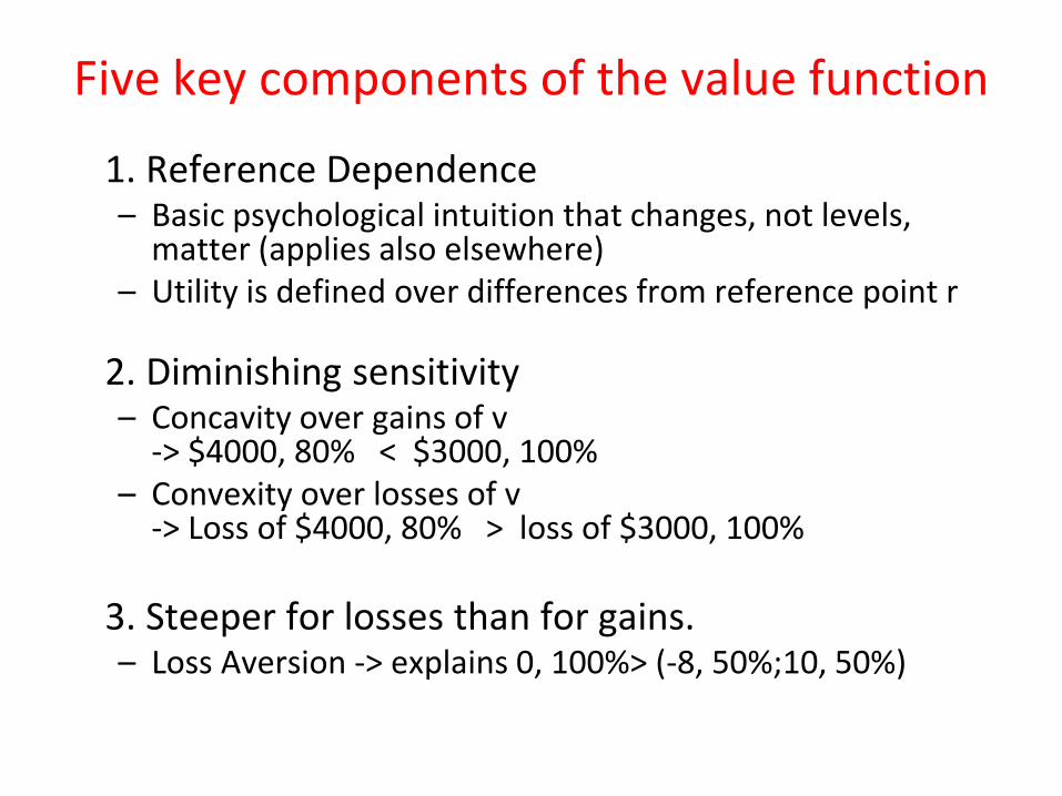
Five key components of the value function

1. Reference Dependence – Basic psychological intuition that changes, not levels,

matter (applies also elsewhere) – Utility is defined over differences from reference point r

2. Diminishing sensitivity

– Concavity over gains of v -> $4000, 80% < $3000, 100%

– Convexity over losses of v -> Loss of $4000, 80% > loss of $3000, 100%

3. Steeper for losses than for gains. – Loss Aversion -> explains 0, 100%> (-8, 50%;10, 50%)

Shape of the value function

4. Probability weighting function π is non-linear

-> explains (5000,.001) > (5,1) and (-5,1) > (-5000,.001) – Overweight small probabilities + Premium for certainty

5. Narrow framing – Consider only risk in isolation

– Neglect other relevant decisions

Five key components

Reference point

• What is the reference point r? • Open question — depends on context

– KT(1979) Status quo or one’s current assets for most of the problems

• Common specification of loss aversion

<−≥−

=; if )(; if

)(rxrxrxrx

xvλ

Experiment: Trade Asymmetry (Knetsch, 1989)

• 3 treatments – Group 1: Granted the mug, offered to exchange

for the candy – Group 2: Granted the candy, offered to exchange

for the mug – Group 3: Granted the choice between the mug

and the candy

• Time to experience the object (questionnaire)

Trade Asymmetry (Knetsch, 1989)

• Result: 90% prefer to keep the original object

Endowment effect (Kahnemann, Knetsch, Thaler 1990)

Random treatment allocation: 50% are sellers and 50% are buyers of a good: 1. induced value tokens (different between subjects) 2. coffee mugs ($6.00, no price tag) 3. pens ($3.98, price tag) Subjects played for 4 rounds and were asked for WTA = willingness to accept (sellers) or WTP = willingness to pay (buyers)

Endowment effect, mugs (Kahnemann, Knetsch, Thaler 1990)

Endowment effect for mugs (Kahnemann, Knetsch, Thaler 1990)

Endowment effect - Relevance - Leads to contradiction of essential economic results

• Indifference curves can intersect (Knetsch, 1990) • Allocation of property rights may affect efficiency

(violates Coase Theorem, 1960)

- Impedes mutually beneficial exchange of various goods (reduces gains from trade)

• Example: lower number of transactions when the housing prices fall

Results from classroom experiment

• An incentive-compatible random-price mechanism was used to elicit the WTA of owners of a chocolate bar and the WTP of non-owners for a chocolate bar

• Findings: Average WTA of sellers: xy euros Average WTP of buyers: xy euros

Possible explanations?

1. Transaction costs 2. Asymmetric information about quality 3. Strategic bidding (but: results for tokens!) 4. Leading explanation

Endowment Effect = Reference-Dependent Preferences +

Loss Aversion

Loss aversion and endowment effect Endowment effect is predicted by reference-dependent utility with loss aversion λ>1

– Assume only gain-loss utility, and assume piece-wise linear formulation (1)+(3)

– Two components of utility: utility of owning the object u(m) and (linear) utility of money p

– Assumption: No loss-aversion over money (experimental evidence)

– WTA: Given mug -> r = {mug}, so selling mug is a loss – WTP: Not given mug -> r = {Ø}, so getting mug is a

gain – Assume u{Ø} = 0

Loss aversion and endowment effect This implies:

– Sellers’ WTA: not selling = selling mug (where r=mug) u{mug} - u{mug} = λ[u{Ø} - u{mug}] + pWTA

pWTA = λu{mug}

– Buyers’ WTP: not buying = buying mug (where r=Ø)

u{Ø} - u{Ø} = u{mug} - u{Ø} - pWTP

pWTP = u{mug}

– It follows that pWTA = λu{mug} = λpWTP

– If loss aversion over money pWTA = λu{mug} = λ²pWTP

<−≥−

=; if )(; if

)(rxrxrxrx

xvλ

Endowment effect: mugs and chocolate?

• Can we generalize the findings to all goods? • Evidence:

– The closer the goods are to money or standard „daily use“ marketable goods, the lower is endowment effect.

– Highest for public goods or non-market goods – Lowest for lotteries and tokens