Lecture 6: Recursive Preferences

Simon GilchristBoston Univerity and NBER

EC 745Fall, 2013

Basics

Epstein and Zin (1989 JPE, 1991 Ecta) following work by Krepsand Porteus introduced a class of preferences which allow tobreak the link between risk aversion and intertemporalsubstitution.

These preferences have proved very useful in applied work inasset pricing, portfolio choice, and are becoming more prevalentin macroeconomics.

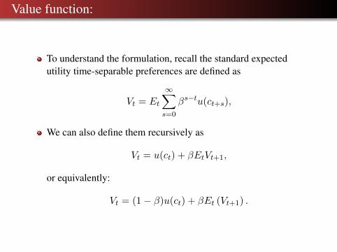
Value function:

To understand the formulation, recall the standard expectedutility time-separable preferences are defined as

Vt = Et

∞∑s=0

βs−tu(ct+s),

We can also define them recursively as

Vt = u(ct) + βEtVt+1,

or equivalently:

Vt = (1− β)u(ct) + βEt (Vt+1) .

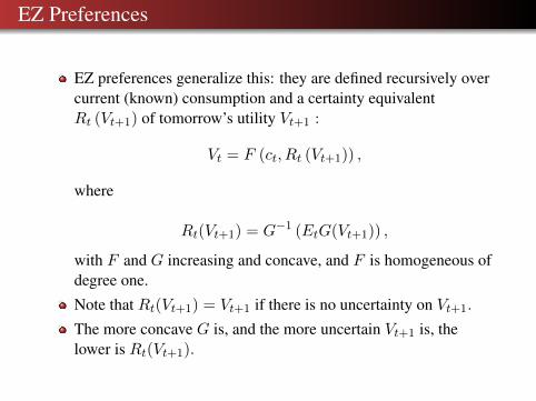
EZ Preferences

EZ preferences generalize this: they are defined recursively overcurrent (known) consumption and a certainty equivalentRt (Vt+1) of tomorrow’s utility Vt+1 :

Vt = F (ct, Rt (Vt+1)) ,

where

Rt(Vt+1) = G−1 (EtG(Vt+1)) ,

with F and G increasing and concave, and F is homogeneous ofdegree one.

Note that Rt(Vt+1) = Vt+1 if there is no uncertainty on Vt+1.

The more concave G is, and the more uncertain Vt+1 is, thelower is Rt(Vt+1).

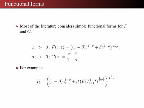
Functional forms

Most of the literature considers simple functional forms for Fand G:

ρ > 0 : F (c, z) =((1− β)c1−ρ + βz1−ρ) 1

1−ρ ,

α > 0 : G(x) =x1−α

1− α.

For example:

Vt =

((1− β)c1−ρ

t + β(EtV

1−αt+1

) 1−ρ1−α

) 11−ρ

.

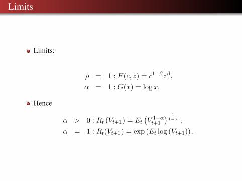
Limits

Limits:

ρ = 1 : F (c, z) = c1−βzβ.

α = 1 : G(x) = log x.

Hence

α > 0 : Rt (Vt+1) = Et(V 1−αt+1

) 11−α ,

α = 1 : Rt(Vt+1) = exp (Et log (Vt+1)) .

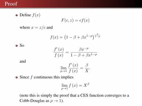
Proof

Define f(x)F (c, z) = cf(x)

where x = z/c and

f(x) =(1− β + βx1−ρ) 1

1−ρ

Sof ′ (x)

f (x)=

βx−ρ

1− β + βx1−ρ

and

limρ→1

f ′ (x)

f (x)=

β

X.

Since f continuous this implies

limρ→1

f (x) = Xβ

(note this is simply the proof that a CES function converges to aCobb-Douglas as ρ→ 1).

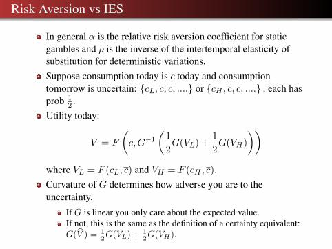
Risk Aversion vs IES

In general α is the relative risk aversion coefficient for staticgambles and ρ is the inverse of the intertemporal elasticity ofsubstitution for deterministic variations.Suppose consumption today is c today and consumptiontomorrow is uncertain: {cL, c, c, ....} or {cH , c, c, ....} , each hasprob 1

2 .

Utility today:

V = F

(c,G−1

(1

2G(VL) +

1

2G(VH)

))where VL = F (cL, c) and VH = F (cH , c).

Curvature of G determines how adverse you are to theuncertainty.

If G is linear you only care about the expected value.If not, this is the same as the definition of a certainty equivalent:G(V̂ ) = 1

2G(VL) + 12G(VH).

Special Case: Deterministic consumption

If consumption is deterministic: we have the usual standardtime-separable expected discounted utility with discount factor βand IES = 1

ρ , risk aversion α = ρ.

Proof: If no uncertainty, then Rt (Vt+1) = Vt+1 andVt = F (ct, Vt+1) . With a CES functional form for F, werecover CRRA preferences:

Vt =(

(1− β)c1−ρt + βV 1−ρ

t+1

) 11−ρ

Wt = (1− β)c1−ρt + βWt+1 = (1− β)

∞∑j=0

βjc1−ρt+j ,

where Wt = V 1−ρt .

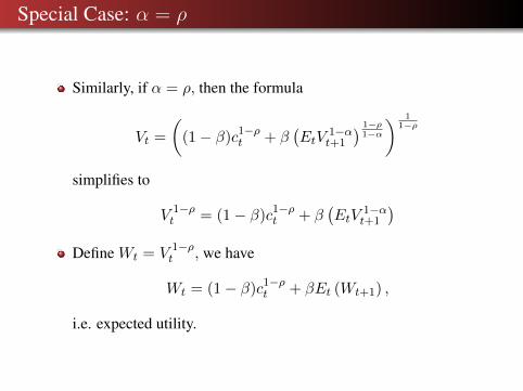
Special Case: α = ρ

Similarly, if α = ρ, then the formula

Vt =

((1− β)c1−ρ

t + β(EtV

1−αt+1

) 1−ρ1−α

) 11−ρ

simplifies to

V 1−ρt = (1− β)c1−ρ

t + β(EtV

1−αt+1

)Define Wt = V 1−ρ

t , we have

Wt = (1− β)c1−ρt + βEt (Wt+1) ,

i.e. expected utility.

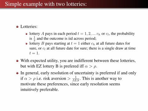
Simple example with two lotteries:

Lotteries:

lottery A pays in each period t = 1, 2, ... ch or cl, the probabilityis 1

2 and the outcome is iid across period;lottery B pays starting at t = 1 either ch at all future dates forsure, or cl at all future date for sure; there is a single draw at timet = 1.

With expected utility, you are indifferent between these lotteries,but with EZ lottery B is prefered iff α > ρ.

In general, early resolution of uncertainty is preferred if and onlyif α > ρ i.e. risk aversion > 1

IES . This is another way tomotivate these preferences, since early resolution seemsintuitively preferable.

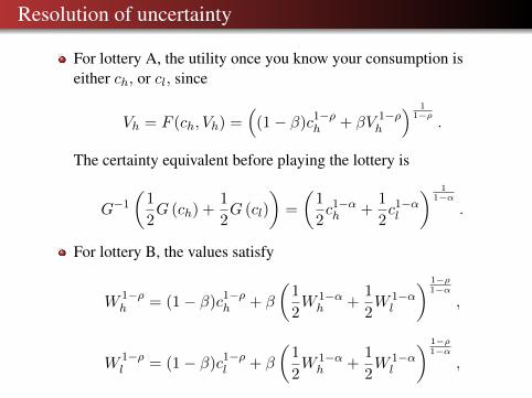
Resolution of uncertainty

For lottery A, the utility once you know your consumption iseither ch, or cl, since

Vh = F (ch, Vh) =(

(1− β)c1−ρh + βV 1−ρ

h

) 11−ρ

.

The certainty equivalent before playing the lottery is

G−1

(1

2G (ch) +

1

2G (cl)

)=

(1

2c1−αh +

1

2c1−αl

) 11−α

.

For lottery B, the values satisfy

W 1−ρh = (1− β)c1−ρ

h + β

(1

2W 1−αh +

1

2W 1−αl

) 1−ρ1−α

,

W 1−ρl = (1− β)c1−ρ

l + β

(1

2W 1−αh +

1

2W 1−αl

) 1−ρ1−α

,

Resolution of uncertainty

We want to compare G−1(

12G (Wh) + 1

2G (Wl))

toG−1

(12G (ch) + 1

2G (cl)).

Note that the function x→ x1−ρ1−α is concave if 1− ρ < 1− α,

i.e. ρ > α, and convex otherwise. As a result, if ρ > α,(1

2W 1−αh +

1

2W 1−αl

) 1−ρ1−α

≥ 1

2

(W 1−αh

) 1−ρ1−α +

1

2

(W 1−αl

) 1−ρ1−α

=1

2W 1−ρh +

1

2W 1−ρl

Also

W 1−ρh ≥ (1− β)c1−ρ

h + β

(1

2W 1−ρh +

1

2W 1−ρl

)W 1−ρl ≥ (1− β)c1−ρ

l + β

(1

2W 1−ρh +

1

2W 1−ρl

)

Continued

These results imply that if ρ > α then

W 1−ρh +W 1−ρ

l

2≥c1−ρh + c1−ρ

l

2.

in which case the certainty equivalent of lottery A is higher thanthe certainty equivalent of lottery B and agents prefer late toearly resolution of uncertainty.

Technically, EZ is an extension of EU which relaxes theindependence axiom. Recall the independence axion is: if x � y,then for any z,α : αx+ (1− α)z � αy + (1− α)z. With EZ,“Intertemporal composition of risk matters”: we cannot reducecompound lotteries.

Euler’s Thereom:

We have

Vt =(

(1− β)C1−ρt + βRt (Vt+1)1−ρ

) 11−ρ

whereRt (Vt+1) =

(Et(V 1−αt+1

)) 11−α

Since Vt is homogenous of degree one, Euler’s thereom implies

Vt = MCtCt + EtMVt+1Vt+1

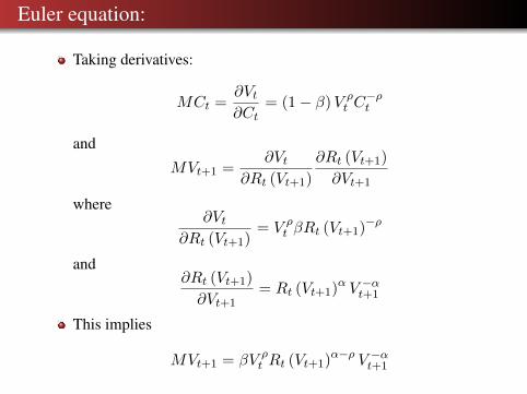
Euler equation:

Taking derivatives:

MCt =∂Vt∂Ct

= (1− β)V ρt C−ρt

and

MVt+1 =∂Vt

∂Rt (Vt+1)

∂Rt (Vt+1)

∂Vt+1

where∂Vt

∂Rt (Vt+1)= V ρ

t βRt (Vt+1)−ρ

and∂Rt (Vt+1)

∂Vt+1= Rt (Vt+1)α V −αt+1

This implies

MVt+1 = βV ρt Rt (Vt+1)α−ρ V −αt+1

IES

Define the intertemporal marginal rate of substitution as

St,t+1 =MVt+1MCt+1

MCt

= β

(Ct+1

Ct

)−ρ( Vt+1

Rt (Vt+1)

)ρ−αThe first term is familiar. The second term is next period’s valuerelative to its certainty equivalent.

If ρ = α or there is no uncertainty so that Vt+1 = Rt (Vt+1) thisterm equals unity.

Household wealth:

Start with the value function:

Vt = MCtCt + EtMVt+1Vt+1

Divide by MCt :

VtMCt

= Ct + Et

(MVt+1MCt+1

MCt

)Vt+1

MCt+1

DefineWt =

VtMCt

thenWt = Ct + EtSt,t+1Wt+1

is the present-discounted value of wealth.

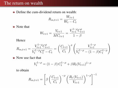
The return on wealth

Define the cum-dividend return on wealth:

Rm,t+1 =Wt+1

Wt − CtNote that

Wt+1 =Vt+1

MCt+1=V 1−ρt+1 C

ρt+1

1− βHence

Rm,t+1 =V 1−ρt+1 C

ρt+1

V 1−ρt Cρt − Ct

=

(Ct+1

Ct

)ρ( V 1−ρt+1

V 1−ρt − (1− β)C1−ρ

t

)Now use fact that

V 1−ρt = (1− β)C1−ρ

t + βRt(Vt+1)1−ρ

to obtain

Rm,t+1 =

[β

(Ct+1

Ct

)−ρ(Rt (Vt+1)

Vt+1

)1−ρ]−1

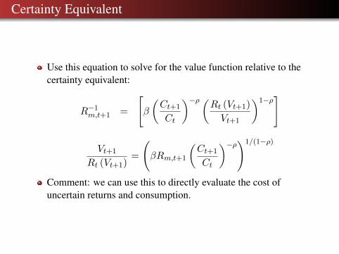
Certainty Equivalent

Use this equation to solve for the value function relative to thecertainty equivalent:

R−1m,t+1 =

[β

(Ct+1

Ct

)−ρ(Rt (Vt+1)

Vt+1

)1−ρ]

Vt+1

Rt (Vt+1)=

(βRm,t+1

(Ct+1

Ct

)−ρ)1/(1−ρ)

Comment: we can use this to directly evaluate the cost ofuncertain returns and consumption.

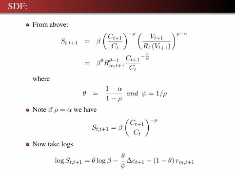
SDF:

From above:

St,t+1 = β

(Ct+1

Ct

)−ρ( Vt+1

Rt (Vt+1)

)ρ−α= βθRθ−1

m,t+1

Ct+1

Ct

− θψ

where

θ =1− α1− ρ

and ψ = 1/ρ

Note if ρ = α we have

St,t+1 = β

(Ct+1

Ct

)−ρNow take logs

logSt,t+1 = θ log β − θ

ψ∆ct+1 − (1− θ) rm,t+1

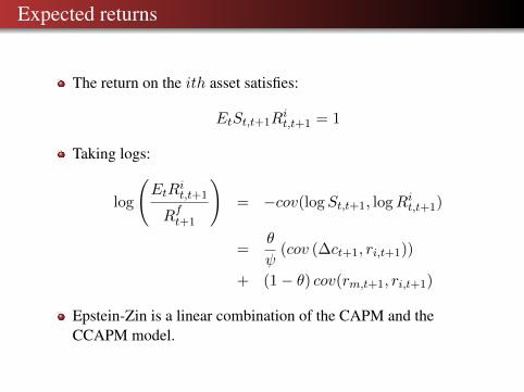
Expected returns

The return on the ith asset satisfies:

EtSt,t+1Rit,t+1 = 1

Taking logs:

log

(EtR

it,t+1

Rft+1

)= −cov(logSt,t+1, logRit,t+1)

=θ

ψ(cov (∆ct+1, ri,t+1))

+ (1− θ) cov(rm,t+1, ri,t+1)

Epstein-Zin is a linear combination of the CAPM and theCCAPM model.

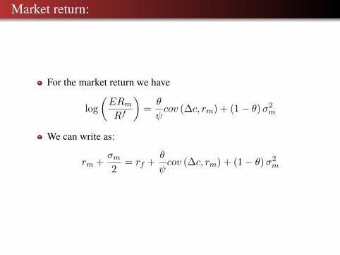
Market return:

For the market return we have

log

(ERmRf

)=θ

ψcov (∆c, rm) + (1− θ)σ2

m

We can write as:

rm +σm2

= rf +θ

ψcov (∆c, rm) + (1− θ)σ2

m

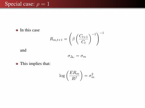
Special case: ρ = 1

In this case

Rm,t+1 =

(β

(Ct+1

Ct

)−1)−1

andσ∆c = σm

This implies that:

log

(ERmRf

)= σ2

m

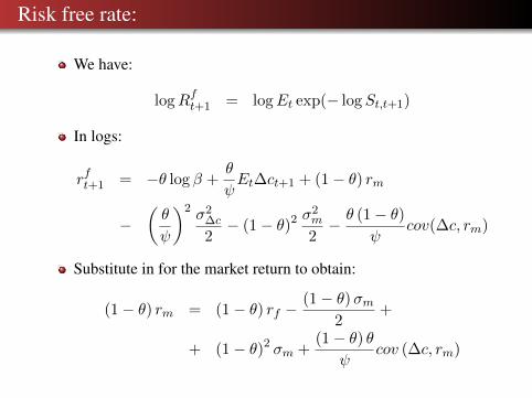
Risk free rate:

We have:

logRft+1 = logEt exp(− logSt,t+1)

In logs:

rft+1 = −θ log β +θ

ψEt∆ct+1 + (1− θ) rm

−(θ

ψ

)2 σ2∆c

2− (1− θ)2 σ

2m

2− θ (1− θ)

ψcov(∆c, rm)

Substitute in for the market return to obtain:

(1− θ) rm = (1− θ) rf −(1− θ)σm

2+

+ (1− θ)2 σm +(1− θ) θ

ψcov (∆c, rm)

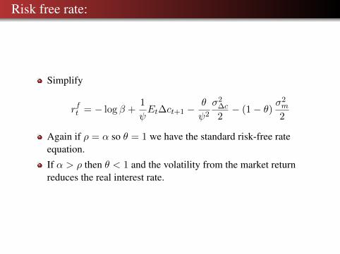
Risk free rate:

Simplify

rft = − log β +1

ψEt∆ct+1 −

θ

ψ2

σ2∆c

2− (1− θ) σ

2m

2

Again if ρ = α so θ = 1 we have the standard risk-free rateequation.

If α > ρ then θ < 1 and the volatility from the market returnreduces the real interest rate.

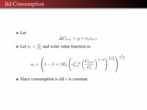
Iid Consumption

Let∆Ct+1 = g + σcεt+1

Let vt = VtCt

and write value function as

vt =

1− β + βEt

(v1−αt+1

(Ct+1

Ct

)1−α) 1−ρ

1−α

11−ρ

Since consumption is iid v is constant.

SDF with iid consumption

With vt = v

St,t+1 = β

(Ct+1

Ct

)−ρ( Vt+1

Rt (Vt+1)

)ρ−α

= β

(Ct+1

Ct

)−α 1

Et

((Ct+1

Ct

)1−α)−(1−θ)

Take logs:

logSt,t+1 = log β − α∆ct+1 + (1− θ) logEt exp((1− α)∆ct+1)

= log β − α∆ct+1 + (α− ρ) g + (1− θ) (1− α)2 σc2

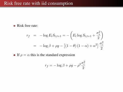
Risk free rate with iid consumption

Risk free rate:

rf = − logEtSt,t+1 = −(Et logSt,t+1 +

σ2s

2

)= − log β + ρg −

[(1− θ) (1− α) + α2

] σ2c

2

If ρ = α this is the standard expression

rf = − log β + ρg − ρ2σ2c

2

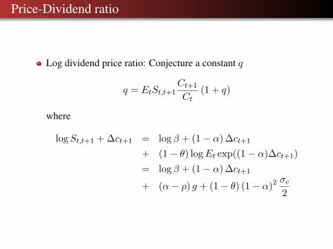
Price-Dividend ratio

Log dividend price ratio: Conjecture a constant q

q = EtSt,t+1Ct+1

Ct(1 + q)

where

logSt,t+1 + ∆ct+1 = log β + (1− α) ∆ct+1

+ (1− θ) logEt exp((1− α)∆ct+1)

= log β + (1− α) ∆ct+1

+ (α− ρ) g + (1− θ) (1− α)2 σc2

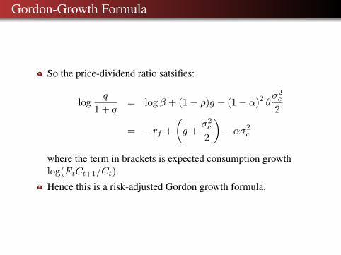
Gordon-Growth Formula

So the price-dividend ratio satsifies:

logq

1 + q= log β + (1− ρ)g − (1− α)2 θ

σ2c

2

= −rf +

(g +

σ2c

2

)− ασ2

c

where the term in brackets is expected consumption growthlog(EtCt+1/Ct).

Hence this is a risk-adjusted Gordon growth formula.

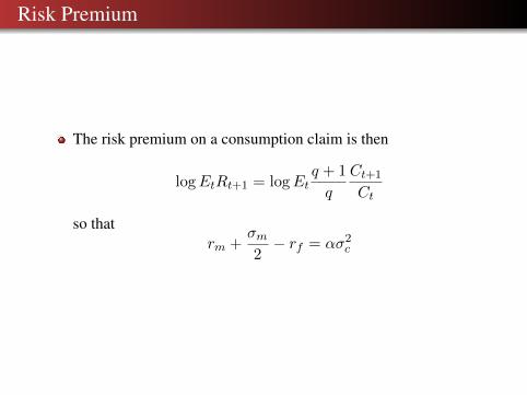
Risk Premium

The risk premium on a consumption claim is then

logEtRt+1 = logEtq + 1

q

Ct+1

Ct

so thatrm +

σm2− rf = ασ2

c

Consumption-Wealth Ratio:

Start with the identity:

Wt+1 = Rm,t+1 (Wt − Ct)

to obtain the log-linear equation:

∆wt+1 = rm,t+1 + k +

(1− 1

ρ

)(ct − wt)

where ρ = 1− exp(c− w).

Rearrange to obtain

(1− ρ) (ct − wt) = ρrm,t+1 − ρ∆wt+1 + ρk

= ρrm,t+1 + ρ [∆ (ct+1 − wt+1)−∆ct+1] + ρk

Present value relationship:

ct − wt = ρ (rm,t+1 −∆ct+1) + ρ (ct+1 − wt+1) + ρk

=

∞∑s=1

ρs [rm,t+s −∆ct+s] +ρ

1− ρk

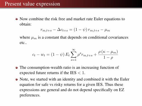
Present value expression

Now combine the risk free and market rate Euler equations toobtain:

rm,t+s −∆ct+s = (1− ψ) rm,t+s − µmwhere µm is a constant that depends on conditional covariancesetc..

ct − wt = (1− ψ)Et

∞∑s=1

ρsrm,t+s +ρ (κ− µm)

1− ρ

The consumption-wealth ratio is an increasing function ofexpected future returns if the IES < 1.

Note, we started with an identity and combined it with the Eulerequation for safe vs risky returns for a given IES. Thus theseexpressions are general and do not depend specifically on EZpreferences.

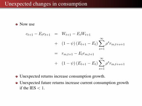
Unexpected changes in consumption

Now use

ct+1 − Etct+1 = Wt+1 − EtWt+1

+ (1− ψ) (Et+1 − Et)∞∑s=1

ρsrm,t+s+1

= rm,t+1 − Etrm,t+1

+ (1− ψ) (Et+1 − Et)∞∑s=1

ρsrm,t+s+1

Unexpected returns increase consumption growth.

Unexpected future returns increase current consumption growthif the IES < 1.

Some comments

If returns are not forecastable, the consumption-wealth ratio is aconstant.

In this case, consumption volatility equals the volatility ofwealth, or equivalently the market return.

In the data this is obviously not true – hence returns must bepredictable.

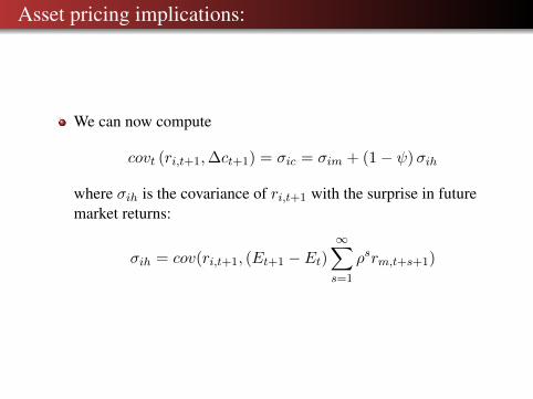
Asset pricing implications:

We can now compute

covt (ri,t+1,∆ct+1) = σic = σim + (1− ψ)σih

where σih is the covariance of ri,t+1 with the surprise in futuremarket returns:

σih = cov(ri,t+1, (Et+1 − Et)∞∑s=1

ρsrm,t+s+1)

Epstein-Zin preferences and Risk Premiums:

Using EZ preferences, the risk premium is:

Etri,t+1 − rf,t+1 +σ2i

2= θ

σicψ

+ (1− θ)σim

The risk premium for asset i depends on its covariance betweencurrent returns and its covariance with news about future marketreturns:

Etri,t+1 − rf,t+1 +σ2i

2= ασim + (α− 1)σih

where α is the coefficient of relative risk aversion.

Note we don’t need to know the IES or consumption growth toprice risk in this framework.

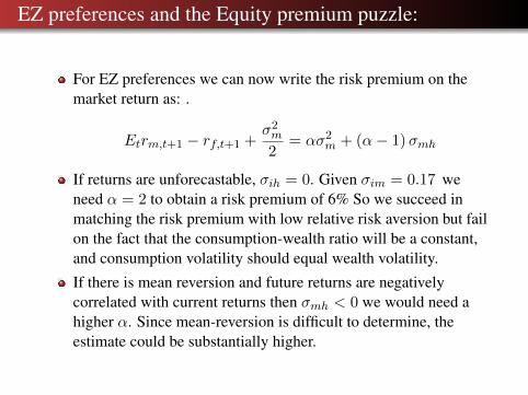
EZ preferences and the Equity premium puzzle:

For EZ preferences we can now write the risk premium on themarket return as: .

Etrm,t+1 − rf,t+1 +σ2m

2= ασ2

m + (α− 1)σmh

If returns are unforecastable, σih = 0. Given σim = 0.17 weneed α = 2 to obtain a risk premium of 6% So we succeed inmatching the risk premium with low relative risk aversion but failon the fact that the consumption-wealth ratio will be a constant,and consumption volatility should equal wealth volatility.

If there is mean reversion and future returns are negativelycorrelated with current returns then σmh < 0 we would need ahigher α. Since mean-reversion is difficult to determine, theestimate could be substantially higher.

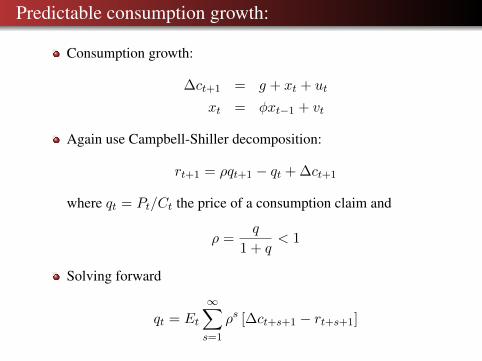
Predictable consumption growth:

Consumption growth:

∆ct+1 = g + xt + ut

xt = φxt−1 + vt

Again use Campbell-Shiller decomposition:

rt+1 = ρqt+1 − qt + ∆ct+1

where qt = Pt/Ct the price of a consumption claim and

ρ =q

1 + q< 1

Solving forward

qt = Et

∞∑s=1

ρs [∆ct+s+1 − rt+s+1]

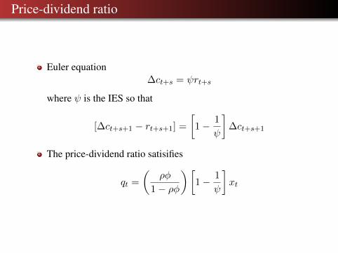
Price-dividend ratio

Euler equation∆ct+s = ψrt+s

where ψ is the IES so that

[∆ct+s+1 − rt+s+1] =

[1− 1

ψ

]∆ct+s+1

The price-dividend ratio satisifies

qt =

(ρφ

1− ρφ

)[1− 1

ψ

]xt

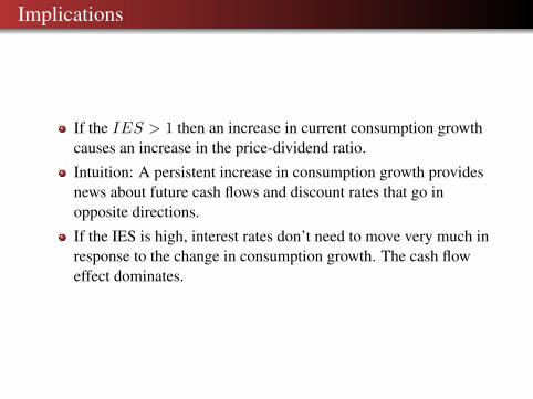
Implications

If the IES > 1 then an increase in current consumption growthcauses an increase in the price-dividend ratio.

Intuition: A persistent increase in consumption growth providesnews about future cash flows and discount rates that go inopposite directions.

If the IES is high, interest rates don’t need to move very much inresponse to the change in consumption growth. The cash floweffect dominates.

Comments

We need a high φ to get large volatility in the price-dividendratio.

But this comes from predictable dividend growth not fromtime-varying returns (the risk free rate is moving but the riskpremium is not).

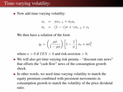
Time-varying volatility:

Now add time-varying volatility:

xt = φxt−1 + σtut

σt = (1− γ)σ + γσt−1 + vt

We then have a solution of the form

qt =

(ρφ

1− ρφ

)[1− 1

ψ

]xt + aσ2

t

where a > 0 if IES > 0 and risk-aversion > 0.We will also get time-varying risk premia – “discount rate news”that offsets the “cash flow” news of the consumption growthshock.In other words, we need time-varying volatility to match theequity premium combined with persistent movements inconsumption growth to match the volatility of the price dividendratio.

Calibration and empirical implementation

Calibration:IES = 1.5, α = 10Very high persistence and volatility for shocks to volatility andperistent consumption-growth process.

Issues to think about:IES > 1 is controversial.Difficult to estimate long-run risk.