PHYS 461 & 561, Fall 2011-2012 110/11/2011

Lecture 6: Entropy Rules! (contd.)

Lecturer:Brigita Urbanc Office: 12-909(E-mail: brigita@drexel.edu)

Course website: www.physics.drexel.edu/~brigita/COURSES/BIOPHYS_2011-2012/

PHYS 461 & 561, Fall 2011-2012 210/11/2011

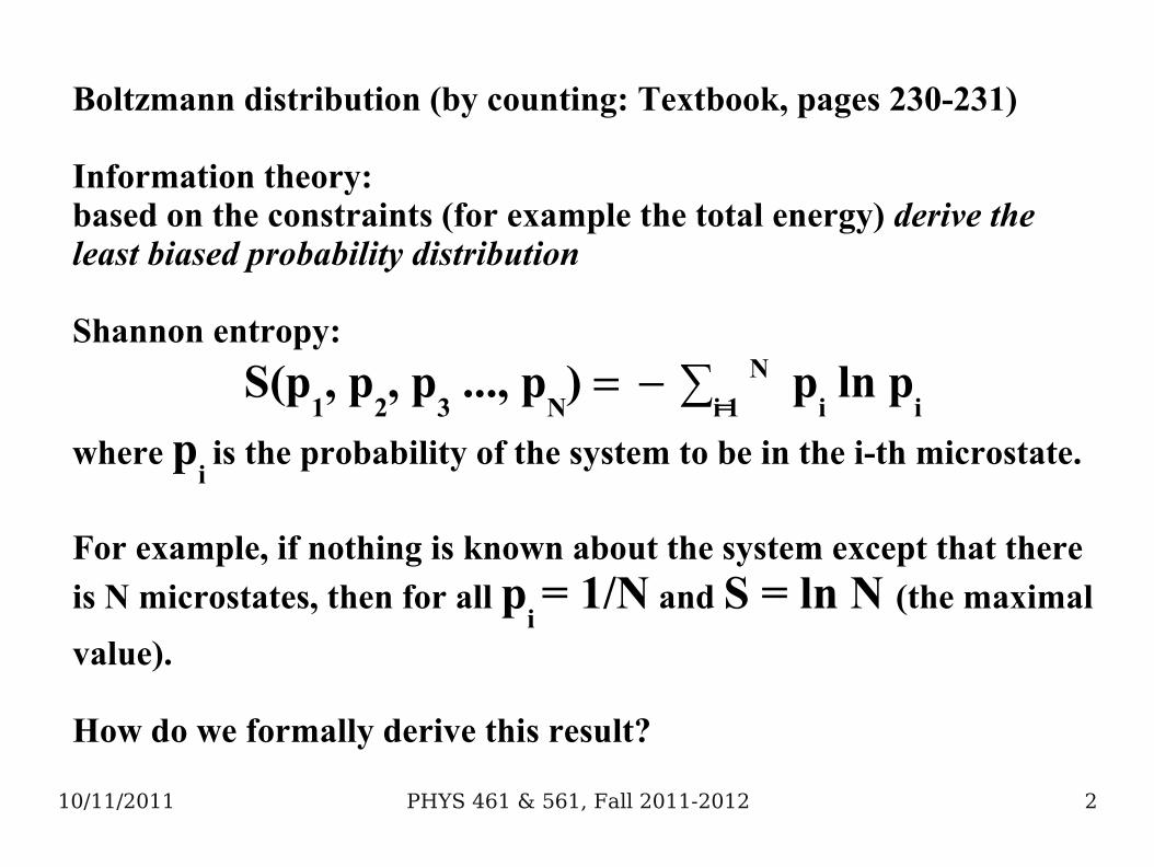
Boltzmann distribution (by counting: Textbook, pages 230-231)

Information theory:based on the constraints (for example the total energy) derive theleast biased probability distribution

Shannon entropy:

S(p1, p

2, p

3 ..., p

N) ∑

i=1

N pi ln p

i

where pi is the probability of the system to be in the i-th microstate.

For example, if nothing is known about the system except that there

is N microstates, then for all pi = 1/N and S = ln N (the maximal

value).

How do we formally derive this result?

PHYS 461 & 561, Fall 2011-2012 310/11/2011

Maximize Shannon entropy S' using Lagrange multiplier method for each constraint:

S' ∑i=1

N pi ln p

i [ ∑

i=1

N pi 1]

Maximization equations:

∂S'/∂ → ∑i=1

N pi 1

∂S'/∂pi → lnp

i 1

pi exp(1

Note that the probabilities pi do not depend on i!

∑i=1

N pi 1 → ∑

i=1

N exp(1 1 → exp(1

pi

PHYS 461 & 561, Fall 2011-2012 410/11/2011

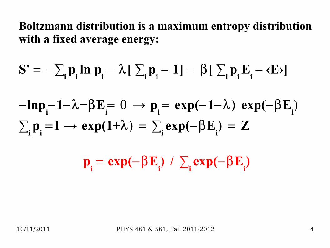
Boltzmann distribution is a maximum entropy distribution with a fixed average energy:

S' ∑i

pi ln p

i [ ∑

i p

i –1] [ ∑

i p

i E

i – ‹E›]

lnpi1 – E

i→p

i exp(1exp(E

i

∑i p

i 1 →exp(1+∑

i exp(E

iZ

pi exp(E

i ∑

i exp(E

i

PHYS 461 & 561, Fall 2011-2012 510/11/2011

Ideal gas approximation: the interaction range is small incomparison to the mean spacing between molecules

For a system with N independent variables (x1, x

2, … x

N)

the probability distribution can be factorized:

P(x1, x

2, … x

N) = P(x

1) P(x

2) … P(x

N)

– uniform spatial distribution of ideal gas molecules.

Microscopic state of the system is

described by (x, px) so the key

information that we need to derive

is P(px) knowing the kinetic

energy of E = px

2/(2m).

PHYS 461 & 561, Fall 2011-2012 610/11/2011

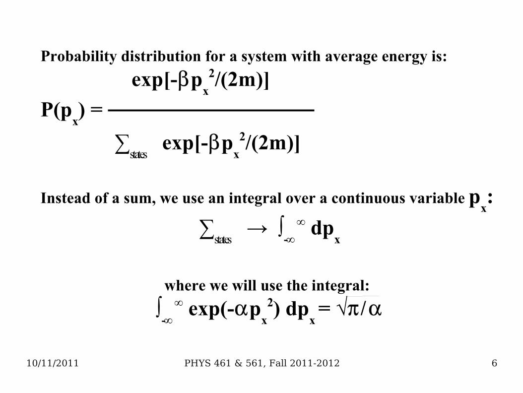
Probability distribution for a system with average energy is:

exp[-px

2/(2m)]

P(px) =

∑states

exp[-px

2/(2m)]

Instead of a sum, we use an integral over a continuous variable px:

∑states

→ ∫-∞

∞ dpx

where we will use the integral:

∫-∞

∞ exp(-px

2) dpx = √

PHYS 461 & 561, Fall 2011-2012 710/11/2011

According to the equipartition theorem, each degree of freedomis associated with :

‹E› = ½ kBT

Calculate ‹E› using the Boltzmann distribution:

Z = ∫-∞

∞ exp[-px

2/(2m)] dpx = √2m

‹› ∫-∞

∞ px

2/(2m) exp[-px

2/(2m)] dpx

We use the following trick:

‹› ∂Z∂½

so we showed that the Lagrange multiplier (kBT) .

PHYS 461 & 561, Fall 2011-2012 810/11/2011

Free energy and chemical potential of a dilute solution:Application of a lattice model (and ideal gas approx.)

PHYS 461 & 561, Fall 2011-2012 910/11/2011

Configurational entropy of N objects placed into W available spots:

!W(N,) = S = k

B lnW

N! (– N)!How to calculate the chemical potential of a dilute solutions?

SOLUTE

= (∂GTOT

/∂NS)

T,p

GTOT

= NW

0

W + N

S

S – T S

MIXwater G + solute energy + mixing entropy contribution

Mixing entropy contribution:-independent solute molecules (ideal gas)

-lattice model: NW

+ NS is a total number of lattice sites

W(NW

,NS) = (N

W + N

S)! / (N

W! N

S!)

PHYS 461 & 561, Fall 2011-2012 1010/11/2011

S = kB lnW = ln[(N

W + N

S)! / (N

W! N

S!)] ≈

kB {N

W ln[N

W/(N

W + N

S)] + N

S ln[N

S/(N

W + N

S)]} =

kB [N

W ln(1 - N

S/N

W) + N

S ln(N

S/N

W)]

Taking into account the Taylor expansion of ln(1+x) ≈ x, we get:

SMIX

= kB [N

S ln(N

S/N

W) – N

S]

GTOT

(T,p,NW

,NS) = N

W

W0 + N

S

S(T,p) +

kBT(N

S ln(N

S/N

W) – N

S)

S(T,p) =

S(T,p) + k

BT ln(c/c

0)

or in a general form expressed in concentration c=N/V:

i =

i0 + k

BT ln(c

i/c

i0)

PHYS 461 & 561, Fall 2011-2012 1110/11/2011

Osmotic pressure Is an Entropic Effect

➔ consider a cell in an aqueous environment exchanging material with a solution (intake of food, excretion of waste)

➔ chemical potential difference proportional to G:

G = (1

2) dN ≤ 0 (spontaneous)

➔ cell with a crowded environment of biomolecules: tendency of almost all components to move out causes a mechanical pressure called osmotic pressure

➔ lipid membranes with ion channels to regulate ion concentration

➔ calculate osmotic pressure due to a dilute solution of NS molecules

PHYS 461 & 561, Fall 2011-2012 1210/11/2011

Osmotic pressure on a semipermeable membrane, which onlyallows water molecules through

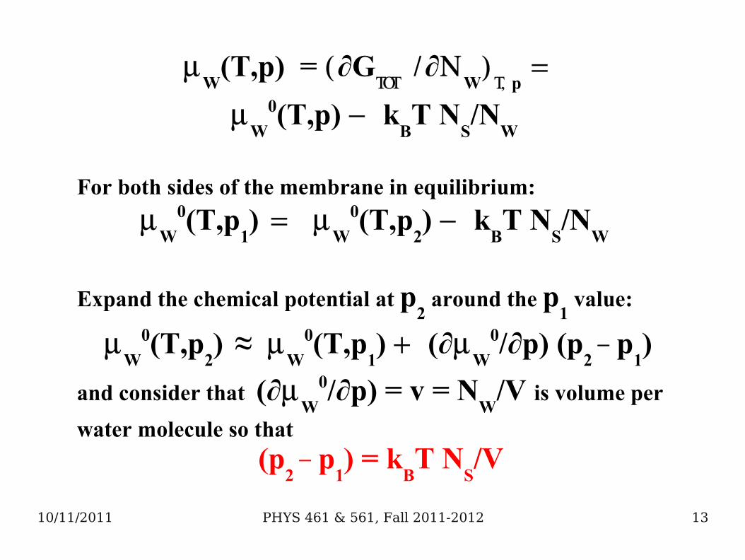
PHYS 461 & 561, Fall 2011-2012 1310/11/2011

W

(T,p) = ∂G

∂W

p

W

0(T,p) kBT N

S/N

W

For both sides of the membrane in equilibrium:

W

0(T,p1)

W

0(T,p2) k

BT N

S/N

W

Expand the chemical potential at p2 around the p

1 value:

W

0(T,p2)

≈

W

0(T,p1) (∂

W

0/∂p) (p2 – p

1)

and consider that (∂W

0/∂p) = v = NW

/V is volume per

water molecule so that

(p2 – p

1) = k

BT N

S/V

PHYS 461 & 561, Fall 2011-2012 1410/11/2011

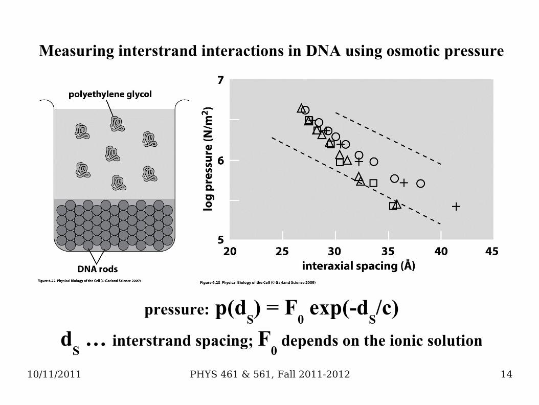
Measuring interstrand interactions in DNA using osmotic pressure

pressure: p(dS) = F

0 exp(-d

S/c)

dS … interstrand spacing; F

0 depends on the ionic solution

PHYS 461 & 561, Fall 2011-2012 1510/11/2011

Law of Mass Action and Equilibrium Constants(Chemical Reactions)

➔ chemical equilibrium between A, B and their complex AB:

A + B AB➔ final equilibrium independent of whether we start with only A and B, or with a high concentration of AB and no A or B

➔ NA, N

B, N

AB … number of A, B, and AB molecules

➔ In equilibrium: dG = 00 = (∂G/∂N

A) dN

A + (∂G/∂N

B) dN

B + (∂G/∂N

AB) dN

AB

➔ A more convenient and general expression:

∑i=1

N i dN

i 0

PHYS 461 & 561, Fall 2011-2012 1610/11/2011

Stoichiometric coefficients for each of the reactants are defined as:

i ±1

depending on whether the number of particles of the i-th type increases or decreases during the reaction:

∑i=1

N i

i 0

∑i=1

N i0

i k

BT ∑

i=1

N ln(ci/c

i0)i

or

∑i=1

N i0

i ln[∏

i=1

N (ci/c

i0)i]

or

∏i=1

N cii = (∏

i=1

N ci0

i) exp(∑i=1

N i0

i)

where we define the equilibrium constant Keq

:

Keq

= (∏i=1

N ci0

i) exp(∑i=1

N i0

i)

PHYS 461 & 561, Fall 2011-2012 1710/11/2011

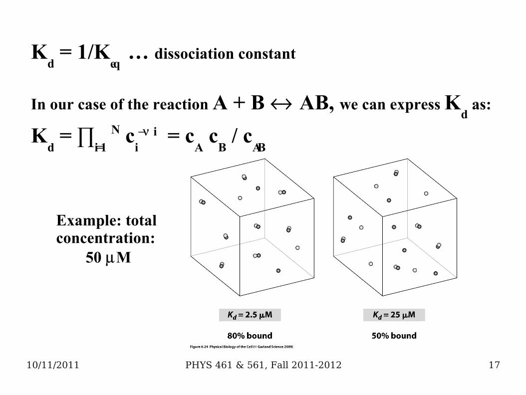
Kd = 1/K

eq … dissociation constant

In our case of the reaction A + B AB, we can express Kd as:

Kd = ∏

i=1

N ci i = c

A c

B / c

AB

Example: total concentration:

50 M

PHYS 461 & 561, Fall 2011-2012 1810/11/2011

Application to Ligand-Receptor Binding:

L + R LRK

d = [L][R]/[LR] or [LR] = [L] [R]/K

d

Binding probability:

[LR] [L]/Kd

pbound

= --------------- = --------------

[LR] + [R] 1 + [L]/Kd

A natural interpretation of Kd: K

d is the concentration at which

the receptor has a probability of ½ of being occupied by a ligand.Based on out prior result, we can express it in terms of lattice

model parameters as: Kd = exp()

PHYS 461 & 561, Fall 2011-2012 1910/11/2011

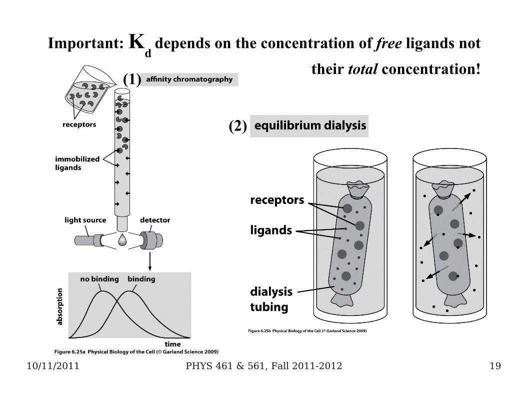
Important: Kd

depends on the concentration of free ligands not

their total concentration!(1)

(2)

PHYS 461 & 561, Fall 2011-2012 2010/11/2011

(C)

(D)

PHYS 461 & 561, Fall 2011-2012 2110/11/2011

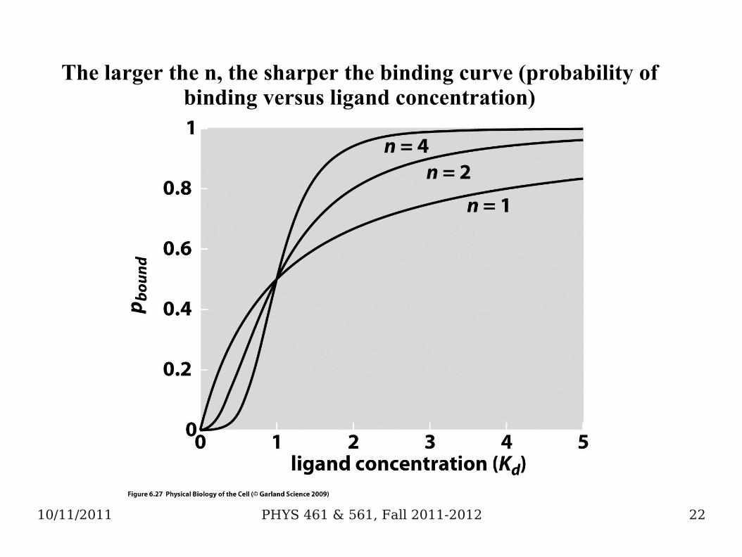
Cooperative Ligand-Receptor Binding: The Hill Function

Biological function: an on-off switch behavior triggered byBinding of a ligand to a receptor involves a cooperative (all-or-none) mechanism:

L + L + R L2R

Kd

2 = [L]2[R]/[L2R]

([L]/Kd)2 ([L]/K

d)n

pbound

= ---------------- = --------------------

1 + ([L]/Kd)2 1 + ([L]/K

d)n

PHYS 461 & 561, Fall 2011-2012 2210/11/2011

The larger the n, the sharper the binding curve (probability ofbinding versus ligand concentration)