lecture 5: tensor-network renormalization group (tnrg)

Lecture 5: Tensor-Network Renormalization Group(TNRG)

Naoki KAWASHIMA

ISSP, U. Tokyo

May 13, 2019

Naoki KAWASHIMA (ISSP) Statistical Machanics I May 13, 2019 1 / 22

In this lecture, we see ...

The MKRG was manageable, but is rather crude an approximation.Even worse, we do not know when we can expect this approximationto be good or how we can improve systematically.

Real-space renormalization group method based on tensor-networkrepresentation (TNRG) provides us with a method for computing thepartition function. While TNRG is also an approximation, it comeswith a method for systematic improvements, and may produce theexact critical exponents in the limit.


[5-1] Tensor-network renormalization group (TNRG)

Most of statistical-mechanical models on lattices are tensor networks.

Quantum many-body states on lattices are also described by tensornetworks.

As we have seen, after renormalization transformation, we needinfinitely many parameters to describe the resulting system.

By working with the TN representation, and introducing “datacompression” at all length scales, we can overcome both the faults inthe real-space RG.


What is a tensor network?

When an object is expressed as the result of (full or partial)contraction of tensor-product of multiple tensors, we call such anexpression a “tensor-network”. An expression such as

Cont

(∏k

T k

)≡∑

(Si )i∈Ω

∏k

T kSik1,S

ik2,··· ,S

iknk

(1)

is a tensor-network, where Ω is a subset of all indices, ikα, appearingmultiple times (typically twice) in the summand.

Example:

TS1,S2,S3,S4 =∑S6,S7,S8,S9

T 1S1,S8,S5

T 2S2,S5,S6

T 3S3,S6,S7

T 4S4,S7,S8


Statistical-mechanical models are tensor networks

The partition function of the Ising model on thesquare lattice can be expressed as

Z =∑S

∏p : shaded square

W (Sip , Sjp , Skp , Slp)

W (S1,S2,S3, S4) ≡ eK(S1S2+S2S3+S3S4+S4S1)

We can regard W (S1,S2, S3,S4) as a degree-4 tensor.

Then, the above equation is a tensor network representation of thepartition function.


Graphical notation

In TN-related discussions, we use more diagrams than equationsbecause it is often much easier to grasp the idea.

For tensors, we often use bulkier symbols than just dots such ascircles, triangles, squares, etc, while we use simple lines for indices.(This is more natural from the information-scientific point of viewbecause tensors are the carriers of most of the information.)


Wave function can be represented as TN (1)

Consider a quantum many-body system defined on a lattice.

A local quantum degree of freedom, say Si , is defined on each site.

Accordingly, we have a local Hilbert space Hi ≡ |Si 〉i associatedwith each site, e.g., Hi is 2-dimensional for S = 1/2 spin models.

The whole Hilbert space is the product of them H ≡⊗

i Hi .

Any global wave function |Ψ〉 can be expanded as

|Ψ〉 ≡∑Si

CS1,S2,··· ,SN |S1, S2, · · · ,SN〉 ≡∑S

CS|S〉

where |S1, S2, · · · ,SN〉 ≡ |S1〉1 ⊗ |S2〉2 ⊗ · · · ⊗ |SN〉N .

Now, CS1,S2,··· ,SN can be viewed as a degree-N tensor. It may beapproximated by some tensor network, i.e,

CS ≈ Cont

(∏k

T k

)


Wave function can be represented as TN (2)

CS ≈ Cont

(∏k

T k

)

=

Note that CS has dN parameters (d = 2 for S = 1/2 spin systems),whereas the tensor network can be specified by only O(N) number ofparameters. By the tensor network representation, we may be able toreduce the computation for large N down to a manageable level.


Trivial Tensor-network RG

Let us condider classical systems, and ask howwe can use the tensor network for RG.

How can we replace the original tensor latticeinto something similar but with the unit cellbigger than the original?

Let us solve this problem starting from the trivialTNRG:

TS1,S2,S3,S4≡

∑S9,S10,S11,S12

T 1S1,S9,S12,S8

× T 2S2,S3,S10,S9

T 3S10,S4,S5,S11

T 4S12,S11,S6,S7

where S1 ≡ (S1,S2), S2 ≡ (S3, S4), · · ·

⇓


What’s wrong with trivial TNRG?

Using T , we can exactly express the originalpartition function with lattice constant twicelarger than the original, which is good.

However, the dimension of each index of the newtensor is χ2 where χ is the index dimension ofthe original tensor.

To be more specific, to handle an L× L systemwe end up with a big tensor with χL-dimensionalindices. (We cannot go to so large L.)

To make the whole procedure practically usefulfor larger systems, we need to make the indexdimension back to χ in each iteration.

Data compression is necessary!


Rank-reducer

What we need is a ‘rank-reducer’.

A rank-reducer is a tensor whose rank (whenviwed as a matrix) is χ in stead of χ2, andwhose insertion keep things unchanged.

If such a thing exists, we can define triangleoperators as illustrated in the figure by SVD.

Then, by cutting the network at the reducedindices, we can define the renormalized tensorwith index dimension χ, as we disired.

Now, we must ask whether such a magicalrank-reducer exists or not, and if it does, how wecan compute it.


Low-rank approximation (LRA)

How can we optimize the rank-reducer X for the given rank χ?

For the cost function, we take the amplitude of the local disturbancecaused by the insertion of X , i.e.,

Let us regard A and B as χ4 × χ2 matrices and the rank-reducer X asa χ2 × χ2 matrix whose rank is χ (or less).

Low-rank approximation problem

Suppose 3 integers, l ,m, n, that satisfy l < m < n. For two given n ×mmatrices A and B, find a rank-l , m ×m matrix X that minimizes

C (X ) ≡ |ABT − AXBT|2. (2)


Solution to LRA problem (1)

We want the rank-l matrix Xthat minimizes

C ≡ |ABT − AXBT|2.

Consider the QR-decomposition,

A = QARA, B = QBRB .

Then, C ≡ |RARTB − RAXR

TB |2

Consider SVD: RARTB = UΛV T.

If X satisfies

RAXRTB = UΛV T, (3)

it is optimal. (∗) (Here, U, Λ,and V are truncated matrices atthe l-th row and/or column.)


Solution to LRA problem (2)

Now, let us define “trianguleoperators,” PA and PB , by

PA ≡ RTB V Λ−

12 ,

PB ≡ RTA UΛ−

12

Then, because RARTB = UΛV T,

RAPA = UΛ12 ,

RBPB = V Λ12 .

Therefore, X ≡ PAPTB , satisfies

Eq.(3), RAXRTB = UΛV T, and

therefore is the optimalrank-reducer.


Supplement: Theorem for Low-Rank Approximation (LRA)

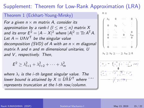
Theorem 1 (Eckhart-Young-Mirsky)

For a given n ×m matrix A, consider itsapproimation by a rank-l (l ≤ m ≤ n) matrix Xand its error E 2 = |A− X |2 where |A|2 ≡ TrATA.Let A = UΛV T be the singular valuedecomposition (SVD) of A with an n×m diagonalmatrix Λ and n and m dimensional unitaries, Uand V , respectively. Then,

E 2 ≥ λ2l+1 + λ2

l+2 + · · ·+ λ2m

where λi is the i-th largest singular value. Thelower bound is attained by X ≡ UΛV T where ’ ’represents truncation at the l-th row/column.

Λ ≡

λ1 0 · · · 0

0 λ2

. . ....

.

.

.. . .

. . . 00 · · · 0 λm0 · · · · · · 0

.

.

.

.

.

.0 · · · · · · 0

.

λ1 ≥ λ2 ≥ · · · ≥ λm ≥ 0


Supplement: LRA used in the derivation

Theorem 2 (LRA)

Consider an m ×m matrix Y expressed as Y = RARTB with RA and RB ,

and consider its SVD, Y = UΛV T . Then, Y ’s optimal LRA of the formRAXR

TB with rank l (l < m) matrix X is obtained when RAXR

TB = UΛV T

.

Proof: When the condition of the theorem is satisfied,

|Y − RAXRTB |2 = |UΛV T − UΛV T|2

= |UΛV T − UΛV T|2 = |Λ− Λ|2 =m∑

k=l+1

λ2k ,

where Λ is Λ with singular values λk (k > l) replaced by 0. Therefore,RAXR

TB saturates the inequality of the EYM theorem.


Summary of the TNRG procedure

1 QR-decomposition of A and B matrices.

A = QARA, B = QBRB

2 SVD. RARTB = UΛV T

3 Compute the “triangle operators”.

PA ≡ RTB V Λ−

12 ,

PB ≡ RTA UΛ−

12

4 Do the same for other directions.

5 Using the triangular operators, contract fouroriginal tensors to obtain the new elementtensor T .

6 Repeat these till the desired system size hasbeen reached.


TNRG provides accurate estimates

The free energy can be obtainedto the accuracy of nearly 8digits. (“TRG” in the figure.)(“TRG” is essentially the same, but technically different

way of realizing TNRG from the one discussed in this

lecture. See Levin and Nave, Phys. Rev. Lett. 99,

120601 (2007) for details.)

An improvement (“TNR”)pushes it even up to 10 digits.

[Evenbly and Vidal, Physical Review Letters

115, 180405 (2015)]


How we can compute other quantities

From the method described so far, we can obtain F ,E ,S and C . Whatabout the magnetization, M, χ, and the Binder ratio?

Define “impurity tensors”,

T (0) ≡ T , T (n) ≡ 0 (n > 1)

T(1)S1S2S3S4

≡ TS1S2S3S4 ×m(S1,S2,S3, S4)

where m = (S1 + S2 + S3 + S4)/2 .

Define “renormalized impurity tensors”:

T (n) ≡∑

n1n2n3n4(∑

k nk=n)

Cont(T (n1)T (n2)T (n3)

×T (n4) × (triangle tensors))

At the end of all iterations,〈Mn〉 =

∑S1S2

T(n)S1S2S1S2

/∑S1S2

T(0)S1S2S1S2


Application of TNRG to q-state Potts model (1)

q-state Potts model in 2D.[S. Morita and N.K., ComputationalPhysics Communications, 236 65-71(2019).]

n-th moments of magnetization arecomputed (e.g., magnetization(n = 1), susceptibility (n = 2),Binder ratio (n = 4), etc)

The result of 20 RG iterations (i.e.,L = 220 ≈ 106) was obtaind forq = 2, 3, · · · , 7 for the truncationdimension (‘bond-dimension’)χ = 48.


Application of TNRG to q-state Potts model (2)

According to the finite-size scaling(FSS), which we will discuss later, theBinder ratio is defined as U4 ≡〈M4〉/〈M2〉2 depends on T and L as(

dU4

dT

)T=Tc

=1

νlog L+a+bL−ω+· · ·

For first-order transitions, 1/ν = d isexpected.

The 1st order nature of the transition of5-state Potts model has beenconfirmed. (CF: ξ ≈ 2500 at Tc).

[S. Morita and N.K., Comp. Phys.

Comm. 236, 65-71 (2019).]


Summary

Tensor-network RG (TNRG) is a scheme that realizes “datacompression” at every length scale.

With TNRG, we can systematically improve the real-space RG byadjusting the compression level, i.e., by increasing the cut-offdimension χ (often called “bond-dimension”).

TNRG provides us with rather accurate estimates of various quantitiesand critical indices.

While we have seen just one way of implementing the idea, there aremany proposals for realizing TNRG. (MERA, TRG, TNR, loop-TNR,etc)


lecture 5: tensor-network renormalization group (tnrg)

Documents