phys 4390: general relativity lecture 6: tensor calculus · phys 4390: general relativity lecture...

PHYS 4390: GENERAL RELATIVITY

LECTURE 6: TENSOR CALCULUS

To start on tensor calculus, we need to define differentiation on a manifold.Agood question to ask is if the partial derivative of a tensor a tensor on a manifold?

∂̃X̃a =∂

∂x̃c

(∂x̃a

∂xbXb

)=

∂xd

∂x̃c∂

∂xd

(∂x̃a

∂xbXb

)=

∂xd

∂x̃c∂2x̃a

∂xd∂xbXb +

∂xd

∂x̃c∂x̃a

∂xb∂Xb

∂xd

=∂xa

∂x̃b∂x̃d

∂xc∂aX

b +∂2x̃a

∂xd∂xb∂xd

∂x̃cXb

This will not be a tensor as the second term involves second derivatives of the newcoordinate system; unless this term is removed or somehow cancelled out, this willnot transform in a tensorial manner.

From calculus we know that the derivative is a limiting process of two functionevaluations at different points

f ′(x) = limh→0

f(x+ h)− f(x)

h.

We are going to consider a similar expression for tensors in analogy to this

limδn→0

[Xa]P − [Xa]Qδn

where δu indicates the separation between P andQ. There is a problem, however, asthe coordinate transformations at these different points will in general be different,since these objects are evaluated at points:

X̃aP =

[∂x̃a

∂xb

]PXbP , and, X̃

aQ =

[∂x̃a

∂xb

]QXbQ.

In order to define a tensorial derivative, we must devise a clever way to ”drag” atensor at one place to another.

1. The Lie Derivative

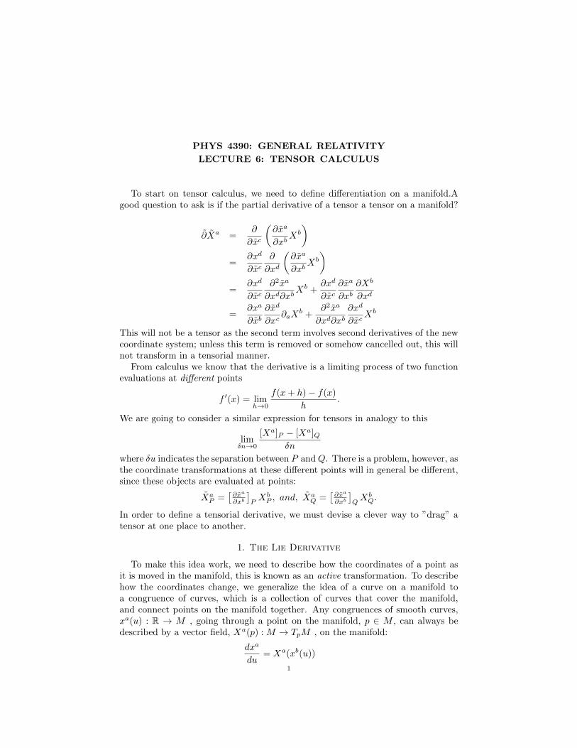
To make this idea work, we need to describe how the coordinates of a point asit is moved in the manifold, this is known as an active transformation. To describehow the coordinates change, we generalize the idea of a curve on a manifold toa congruence of curves, which is a collection of curves that cover the manifold,and connect points on the manifold together. Any congruences of smooth curves,xa(u) : R → M , going through a point on the manifold, p ∈ M , can always bedescribed by a vector field, Xa(p) : M → TpM , on the manifold:

dxa

du= Xa(xb(u))

1

2 PHYS 4390: GENERAL RELATIVITY LECTURE 6: TENSOR CALCULUS

Figure 1. A congruence of curves on a manifold M

With these curves, we will be able to move a tensor at one position P to anotherat Q. Given a particular vector-field Xa associated with a congruence of curves,consider

xa → x̃a = xa + δuXa(x)

we will treat this as a shift from position P to Q, thus the vector X may be seen

as ~PQ for infinitesimally close points P and Q. Computing the first derivatives,

∂x̃a

∂xb= δab + δu∂bX

a

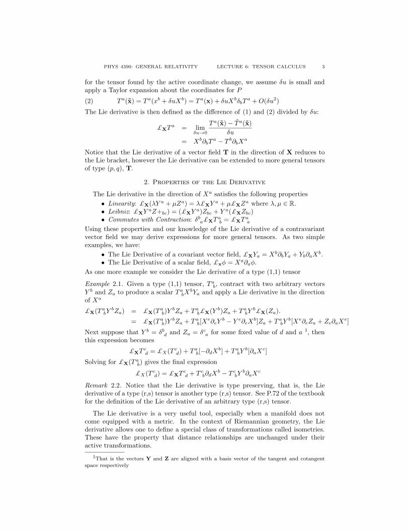
Let us consider the effect of a contravariant rank 1 tensor (or vector field) underthe process of ”dragging”

T a(x)→ T̃ a(x̃)

Figure 2. A vector T a being dragged along a curve generated byXa from P to Q on a manifold

We will also have a second tensor at Q given by the tensor found from the ac-tive coordinate change, T a(x̃) - where we note that T̃ a(x̃) and T a(x̃) are distinctcontravariant vectors.

Since T̃ a(x̃) is a tensor,

T̃ a(x̃) =∂x̃a

∂xbT b(x)

= (δab + δu∂bXa)T b(x)

= T a(x) + [∂bXaT b(x)]δu;(1)

PHYS 4390: GENERAL RELATIVITY LECTURE 6: TENSOR CALCULUS 3

for the tensor found by the active coordinate change, we assume δu is small andapply a Taylor expansion about the coordinates for P

T a(x̃) = T a(xb + δuXb) = T a(x) + δuXbδbTa +O(δu2)(2)

The Lie derivative is then defined as the difference of (1) and (2) divided by δu:

£XTa = lim

δu→0

T a(x̃)− T̃ a(x̃)

δu

= Xb∂bTa − T b∂bXa

Notice that the Lie derivative of a vector field T in the direction of X reduces tothe Lie bracket, however the Lie derivative can be extended to more general tensorsof type (p, q), T.

2. Properties of the Lie Derivative

The Lie derivative in the direction of Xa satisfies the following properties

• Linearity: £X(λY a + µZa) = λ£XYa + µ£XZ

a where λ, µ ∈ R.• Leibniz: £XY

aZ+bc) = (£XYa)Zbc + Y a(£XZbc)

• Commutes with Contraction: δba£XTab = £XT

aa

Using these properties and our knowledge of the Lie derivative of a contravariantvector field we may derive expressions for more general tensors. As two simpleexamples, we have:

• The Lie Derivative of a covariant vector field, £XYa = Xb∂bYa + Yb∂aXb.

• The Lie Derivative of a scalar field, £xφ = Xa∂aφ.

As one more example we consider the Lie derivative of a type (1,1) tensor

Example 2.1. Given a type (1,1) tensor, T ab, contract with two arbitrary vectorsY b and Za to produce a scalar T abX

bYa and apply a Lie derivative in the directionof Xa

£X(T abYbZa) = £X(T ab)Y

bZa + T ab£X(Y b)Za + T abYb£X(Za).

= £X(T ab)YbZa + T ab[X

e∂eYb − Y e∂eXb]Za + T abY

b[Xe∂eZa + Ze∂aXe]

Next suppose that Y b = δbd and Za = δca for some fixed value of d and a 1, thenthis expression becomes

£XTcd = £X(T cd) + T ab[−∂dXb] + T abY

b[∂aXc]

Solving for £X(T ab) gives the final expression

£X(T cd) = £XTcd + T cb∂dX

b − T cbY b∂aXc

Remark 2.2. Notice that the Lie derivative is type preserving, that is, the Liederivative of a type (r,s) tensor is another type (r,s) tensor. See P.72 of the textbookfor the definition of the Lie derivative of an arbitrary type (r,s) tensor.

The Lie derivative is a very useful tool, especially when a manifold does notcome equipped with a metric. In the context of Riemannian geometry, the Liederivative allows one to define a special class of transformations called isometries.These have the property that distance relationships are unchanged under theiractive transformations.

1That is the vectors Y and Z are aligned with a basis vector of the tangent and cotangentspace respectively


While the Lie derivative allows us to define the derivative of a tensor, it is notquite what we want. This definition requires the choice of a vector field X in orderto evaluate the definition of the Lie deriative of a tensor field T. Furthermore thetype preserving nature means this is not quite analogous to applying ∂a - althoughwe may choose coordinates os that it appears this way.

We will see that the covariant derivative will have the properties we want. How-ever in order to discuss this derivative, we must define a new structure on ourmanifold, called a connection which will allow us to ”parallel transport” vectors.

3. Parallel Transport

As a thought experiment, consider an arrow being moved along a closed pathstarting and ending at the same point p, with the arrow pointing in some initialfixed direction for the plane and sphere respectively.

Figure 3. Moving a fixed arrow along a rectangle in the plane R2

On the plane, we may simply consider a rectangle of length m and n. Moving thearrow along this closed path, there will be no change in the direction of the arrow.

For the sphere we will choose a triangle as the closed path for the arrow2.

Figure 4. Moving a fixed arrow along a triangle on the sphere S2

2What happens if the arrow travels along a triangle in the plane, and is there any differenceto a rectangle?


Choosing the initial point p to be the North pole, the arrow travels to the equator,then to a second point along the equator, and then back to the North pole. Despitetravelling in the same manner as the arrow in the plane, the starting and endingvector on the sphere no longer line-up! This change is caused by the basis vectorson the sphere changing from point to point.

While we used congruences of curves to transport tensors to define the Lie de-rivative, this is not the only way to move tensors. Suppose we are given two pointsP = P (x) and Q = Q(x + δx), we would like to define a one-to-one map betweenthe tangent spaces Tp(M) and TQ(M), with the following properties:

• When P = Q the map must reduce to the identity.• The transformation rule is linear 3

We will call the corresponding vectors in TQ(M) parallel.Denoting a vector at P by Xa(x) we define the transported vector at Q as

Xa(x) + δ̄Xa(x).

Linearity ensures that we can write the secon term as

δ̄Xa = W abX

b

where W ab depends on the choice of P and Q. Both requirements can be satisfied

by setting4

W ab = −Γabcδx

c

since limδx→0Wab = 0 for ∀ a, b ∈ [1, n] ensuring the identity map when P = Q.

For the transported vector at Q,

Xa(x) + δ̄Xa(x) = (δab − Γabcδxc)Xb

the Γabc must depend only on P, while the separation to Q is expressed throughδxc. For an n-dimensional manifold Γabc corresponds to n3 functions. The Γabc arecalled connection coefficients and taken together these define a connection. For agiven manifold there are many choices of connection.

4. The Covariant Derivative

To define a derivative we will also need to consider a vector field evaluated atQ = x + δx, using a Taylor expansion

Xa(x + δx) = Xa(x) + δxb∂bXa +O(δx2)

Given Xa(x + δx) and the transported vector Xa(x) + δ̄Xa(x) we now define thecovariant derivative:

∇cXa = limδx→0

1

δxc[Xa(x + δx)− (Xa(x) + δ̄Xa(x))

].

As this is a sum of vectors evaluated at Q, this is an acceptable tensorial definition.Taking the limit δx = 0 this becomes

∇cXa = ∂cXa + ΓabcX

b.

Remark 4.1. The covariant derivative of a vector Xa is also written as Xa;c or xa||c.

3This is the simplest transformation we can pick, and it will ensure our map is one-to-one4The negative sign is included to follow notational convention


The requirement that ∇cXa must be a tensor will constrain how the Γabc trans-form. To see this consider the covariant derivative of X in a new coordinate system

∇̃cX̃a =∂x̃a

∂xb∂xd

∂x̃c(∂dX

b + ΓbedXe) = ∂̃cX̃

a + Γ̃abcX̃b

Expanding out ∂̃cX̃a we may derive an equation for the Γ̃abc:

Γ̃abc =∂x̃a

∂xd∂xe

∂x̃b∂xf

∂x̃cΓdef −

∂xd

∂x̃b∂xe

∂x̃c∂2x̃a

∂xd∂xe

Equivalently, since ∂d(∂xa

∂x̃c∂x̃c

∂xb ) = ∂d(δab) = 0

Γ̃abc =∂x̃a

∂xd∂xe

∂x̃b∂xf

∂x̃cΓdef +

∂x̃a

∂xd∂2x̃d

∂x̃b∂x̃c

Anyt set of functions that transform according to this transformation law is calledan affine connection.

Remark 4.2. The second term compensates for the additional components associ-ated with the partial derivatives under coordinate changes.

5. Properties of the Covariant Derivative

The covariant derivative has some useful properties, just like the Lie derivative

• ∇a is linear.• ∇a satisfies the Liebniz property.• ∇a commutes with contraction.

Using these properties we may show that

• For any scalar field φ, ∇aφ = ∂aφ• The covariant derivative of a covariant vector field is

∇aXb = ∂AXb − ΓcbaXc

• A general type (r,s) tensor has the covariant derivative

∇cT a1,...,arb1,...,bs= ∂cT

a1,...,arb1,...,bs

+ Γa1dcTd,...,arb1,...,bs

+ ...+ ΓardcTa1,...,db1,...,bs

−ΓdbcTa1,...,ard,...,bs

− ...− ΓdbcTa1,...,arb1,...,d

While Γabc is not a tensor, and neither is a sum of two connections, the differenceof two connections is a tensor of type (1,2) .

If the manifold is equipped with a metric gab so that one may form a line element,then there is a unique connection satisfying two properties ∇cgab = 0 and that thisconnection is torsion-free, that is the torsion tensor vanishes. For the moment wewill focus on the second condition, and state without proof that the torsion-freecondition is equivalent to

T abc = Γabc − Γacb = 0

For vanishing torsion, this implies that the connection coefficients must be sym-metric in the lower indices

Γabc = Γacb

With the covariant derivative defined we may extend the definition of the totalderivative, d

du , to consider the absolute derivative. For any congruence of curves


xa(u) defined by the tangent vector Xa(x(u)) through the first order differentialequation

dxa(u)

du= Xa(x(u))

the absolute derivative of a tensor T a1,...,arb1,...,bsis

D

Du(T a1,...,arb1,...,bs

) = ∇XTa1,...,arb1,...,bs

= Xc∇cT a1,...,arb1,...,bs

The definition of parallel propagation may be expressed simply as the vanishing ofthe absolute derivative

D

Du(T a1,...,arb1,...,bs

) = 0

Further, for a vector field λa(u) along the curves xa(u)

D

Du(λa) =

dxb

du∇bλa

=dxb

du(∂bλ

a + Γacbλc)

=dxb

du

∂λa

∂xb+ Γacbλ

c dxb

du

=dλa

du+ Γacbλ

c dxb

du.

This shows the relationship between the total and absolute derivative.

6. Geodesics

In words, we can describe a geodesic as ”the shortest distance between two pointsin a straight line” While we have not really examined distance on a manfiold, wecan still consider the idea of a ”straight line” in a manifold. For a straight line, thetangent vector along the curve must be transported to be a copy of itself multipliedby a function β(u)

D

Du

(dxa

du

)= β(u)

dxa

du

expanding this out we find

d2xa

du2+ Γabc

dxb

du

dxc

du= β(u)

dxa

duthis defines an affine geodesic.

If we can find a parametrization, s, to make β(u) vanish then this becomes

D

Ds

(dxa

ds

)= 0,

or equivalently

d2xa

du2+ Γabc

dxb

du

dxc

du= 0.

Such a parameter s is called an affine parameter. Any transformation s → s′ =as + b will maintain this differential equation with s → s′; we call such a map, anaffine transformation Geodesics will play a fundamental role in General Relativity.They define the paths that freely falling objects take, as well as photons.

phys 4390: general relativity lecture 6: tensor calculus · phys 4390: general relativity lecture...

Documents