lecture 5: revenue managementtransp-or.epfl.ch/courses/decisionaid2012/slides/lecture5.pdf ·...
TRANSCRIPT

Decision aid methodologies in transportation
Lecture 5: Revenue Management
Prem Kumar
Transport and Mobility Laboratory
* Presentation materials in this course uses some slides of Dr Nilotpal Chakravarti and Prof Diptesh Ghosh

Summary
● We learnt about the different scheduling models
● We learnt to formulate these sub-problems into mathematicalmodels
● We learnt to solve problems with different techniques such asheuristics, branch and bound, tree search and column generation
● The models that we learnt so far assumed a fixed system capacityand a known demand pattern
● Eventually capacity is assigned to the demand in such a way that therevenue (or profits) are optimized
● So the moral of the story so far – demand is a “holy cow” while it isonly the supply that can be “flogged around”!

What is Revenue Management?
● Let us dissect our “holy cow” with a new dimension
● Revenue Management in most literature is defined as the art orscience of selling the right supply (seats, tickets, etc.) to the rightdemand (customers) at the right time
● So far, we only talked about supply assignment to demand, but nowwhat is this “right” qualifier?
● What is the right timing?

● Consider the following simple example:
Downward slopingdemand curveD = 100 - P
What price willmaximize revenue ?
Revenue Management: Example
20 40 60 80 100 120
Price
20
40
60
80
100
120
Demand
0

● Consider the following simple example:
Downward slopingdemand curveD = 100 - P
Revenue is maximized when price = 500
Demand = 500
Revenue = 50 x 50 = 2,500
Revenue Management: Example
20 40 60 80 100 120
Price
20
40
60
80
100
120
Demand
0

PRICE DEMAND
1 99
2 98
… …
98 2
99 1
Revenue Management: Example

• Suppose we could sell the product to each customer at the price he is “willing” to pay!
• Then total revenue would be 99 + 98 + … + 1
= 4,950
Revenue Management: Example

PRICE DEMAND
80 20
60 20
40 20
20 20
TOTAL REVENUE 4000
Revenue Management: Example
● Even partial segmentation helps:
● National Car Rental reportedannual incremental revenueof $ 56 million on a base of $750 million – a revenue gainof over 7%
● RM allowed National CarRental to avoid liquidationand return to profitability inless than one year
Revenue Management: Success Stories

● Delta Airline reported annualincremental revenue of $ 300 millionfrom an investment of $ 2 million – a ROIof 150%
● American Airlines reported revenue gainof $ 1.4 billion over a 3 year period.
● Austrian Airlines reported revenue gainsof 150 million Austrian Schillings in 1991-92, in spite of a decrease in Load Factor
● People’s Express did not use RM – andceased to exist
Revenue Management: Success Stories

● National BroadcastingCorporation implemented aRM system for about $ 1 mio.
● It generated incrementalrevenue of $ 200 mio on abase of $ 9 bio in 4 years. Thisis a revenue gain of over 2%and ROI of 200%
Revenue Management: Success Stories

Hotels, Cruise, Casinos, Cargo, Railways…

Revenue Management: When it works
● Perishable product or service
● Fixed capacity
● Low marginal cost
● Demand fluctuations
● Advanced sales
● Market Segmentation

● Your first chance for hands on RM!
● How many seats should be allocated to Y and B fare classes respectively? You decide!
Fare AllocationY 300 ?
B 120 ?140
Revenue Management: Exercise

● Before you can determine the allocations to buckets you need to forecast the demand for each
● Do we need to forecast the demand for both Y and B classes?
● If Y demand came first RM would be unnecessary
● Just sell seats on a First Come First Served basis!
● Since B demand comes first we need to forecast Y demand and allocate inventory accordingly
● Forecasts should be accurate
● High forecasts spoilage
● Low forecasts spillage
Revenue Management: Demand Forecasting

● Objective: Obtain quick and robust forecasts.
● Number of forecasts: Typically around
● 10,000 fare class demand forecasts, or
● 2,000,000 OD demand forecasts
● every night for medium-sized airlines
Revenue Management: Demand Forecasting

● Booking curve, Cancellation curve
● No-shows, Spill, and Recapture
● Revenue values of volatile products
● Up-selling and cross-selling probabilities
● Parameters in the demand function
● Price elasticity of demand
What do we forecast?
Revenue Management: Demand Forecasting

● Time Series Methods
● Moving Averages
● Exponential Smoothing
● Regression
● Pick-Up Forecasting
● Neural Networks
● Bayesian Update Methods
Revenue Management: Demand Forecasting

Forecasting Methods
0
2
4
6
8
10
12
14
16
18
0 5 10 15 20 25
Original Time Series

Forecasting Methods
Time Series (Seasonality Removed)
0
2
4
6
8
10
12
14
16
0 5 10 15 20 25

Time Series (Trend Removed)
0
2
4
6
8
10
12
0 5 10 15 20 25
Forecasting Methods

Moving Averagek period moving average: Take the average of the lastk observations to predict the next observation
0
2
4
6
8
10
12
0 5 10 15 20 25
3-period moving average
Forecasting Methods

Exponential Smoothing
Tomorrow’s forecast = Today’s forecast +
α Error in today’s forecast.
Forecasting Methods

Exponential Smoothing ( =0.3)
0
2
4
6
8
10
12
0 5 10 15 20 25
Forecasting Methods

Exponential Smoothing ( =0.7)
0
2
4
6
8
10
12
0 5 10 15 20 25
Forecasting Methods

145
150
155
160
165
170
175
180
185
14 15 16 17 18 19 20 21
Bookings 90 days prior
Fin
al B
oo
kin
gs
Regression
Forecasting Methods

145
150
155
160
165
170
175
180
185
14 15 16 17 18 19 20 21
Bookings 90 days prior
Fin
al B
oo
kin
gs
Regression
Forecasting Methods

Pick-Up Forecasting
-8 -7 -6 -5 -4 -3 -2 -1 0
6 3 11 4 9 8 13 3 13 9-Apr
8 6 6 3 16 11 5 4 2 10-Apr
1 2 0 0 3 6 2 6 8 11-Apr
6 0 4 1 2 6 3 2 ? 12-Apr
3 8 8 7 5 1 2 ? 13-Apr
1 0 2 6 6 4 ? 14-Apr
0 1 1 6 5 ? 15-Apr
1 11 12 6 ? 16-Apr
Days Prior to Usage Usage
Date
Forecasting Methods

Neural Networks
Input Layer
Hidden Layer
Output Layer
Past Data
Forecasts
Forecasting Methods

The Problem
True Demand
22
15
24
33
16
26
22
23
22
17
Booking Limits
24
20
17
35
16
22
22
15
22
17
Observed Demand
22
15
17
33
16
22
22
15
22
17
Unconstraining
Forecasting Methods: Unconstraining

The Method (The EM Algorithm)
Observed Demand
22
15
17
33
16
22
22
15
22
17
Find the mean and the Standard deviation of thenon-truncated demand:
Mean (m) = (22+15+33+…+17)/7= 21
Std. Dev. (s) = 6.11
Forecasting Methods: Unconstraining

The Method (The EM Algorithm)
Observed Demand
22
15
17
33
16
22
22
15
22
17
Unconstraining 17:
17
Forecasting Methods: Unconstraining

The Method (The EM Algorithm)
Observed Demand
22
15
17
33
16
22
22
15
22
17
Unconstraining 17:
17
Forecasting Methods: Unconstraining

The Method (The EM Algorithm)
Observed Demand
22
15
23.64
33
16
22
22
15
22
17
In a similar manner, handle the unconstraining of 22 and 15.
Forecasting Methods: Unconstraining

The Method (The EM Algorithm)
Observed Demand
22
15
23.64
33
16
26.53
22
22.79
22
17
True Demand
22
15
24
33
16
26
22
23
22
17
Forecasting Methods: Unconstraining

The Method (The EM Algorithm)
Constraineddemand Unconstrained
demand
demand
pro
bab
ility
Forecasting Methods: Unconstraining

Revenue Management: Inventory Allocation
● Airlines have fixed capacity in the short run
● Airline seats are perishable inventory
● The problem - How should seats on a flight be allocated todifferent fare classes
● Booking for flights open long before the departure date -typically an year in advance
● Typically low yield passengers book early

● Leisure passengers are price sensitive and book early
● Business passengers value time and flexibility and usuallybook late
● The Dilemma - How many seats should be reserved for highyield demand expected to arrive late?
● Too much spoilage - the aircraft departs which empty seatswhich could have been filled
● Too little spillage - turning away of high yield passengersresulting in loss of revenue opportunity
Revenue Management: Inventory Allocation

LOAD FACTOR EMPHASIS
YIELD EMPHASIS
REVENUE EMPHASIS
Seats sold For $ 1000
80 248 192
Seats sold For $ 750
280 40 132
TOTAL 360 288 324
LOAD FACTOR 90% 72% 81% REVENUE 290,000 278,000 291,000
YIELD 805 965 898
Need a Revenue Management System to balance load factor and yield
400 Seat Aircraft - Two Fare Classes(Example from Daudel and Vialle)
Load Factor versus Yield Emphasis
120 seats
Three fare classes, CHF 250, CHF 150, & CHF 100
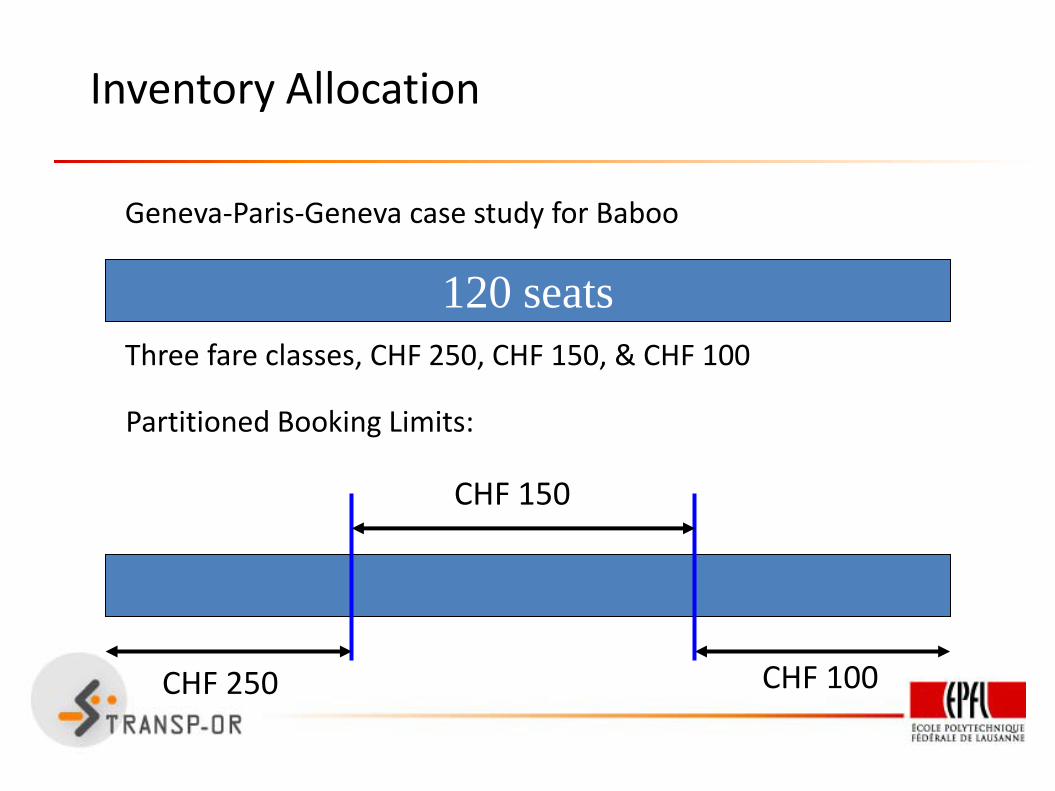
Partitioned Booking Limits:
CHF 250
CHF 150
CHF 100
Inventory Allocation
Geneva-Paris-Geneva case study for Baboo

120 seats
Three fare classes, CHF 250, CHF 150, & CHF 100
Nested Booking Limits:
CHF 250CHF 150
CHF 100
Inventory Allocation: Nesting

CHF 250
CHF 150
CHF 100
Protected for250 fare
class
Protected for250 & 150 fare
class
Inventory Allocation: Protection levels

● Total number of seats: 120
● Seats divided into two classes based on fare: CHF 250 and CHF 150.
● Demands are distinct.
● Low fare class demand occurs earlier than the high fare class demand.
Inventory Allocation: Two-class model

Demand
Pro
bab
ility
Higher Fare Class= 40, = 15
Fare = CHF 250
Lower Fare Class= 80, = 30
Fare = CHF 150
Inventory Allocation: Two-class model

45 seats have already been booked in the lower fare class. Should we allow the 46th booking in the same class?
Inventory Allocation: Two-class model

Revenue from the lower fare class:RL = CHF150
Revenue from the higher fare class:RH = CHF 0 if the higher fare demand < 74,
CHF 250 otherwise.
Expected Revenue from the higher fare class:E(RH) = CHF 0 P(higher fare demand < 74)
+ CHF250 P(higher fare demand 74)
Inventory Allocation: Two-class model

Revenue from the lower fare class:RL = CHF150
Revenue from the higher fare class:RH = CHF 0 if the higher fare demand < 74,
CHF 250 otherwise.
Expected Revenue from the higher fare class:E(RH) = CHF 0 0.9883 (Normal tables)
+ CHF250 0.0117 (Normal tables)CHF 3
Inventory Allocation: Two-class model

0.00
50.00
100.00
150.00
200.00
250.00
0 20 40 60 80 100 120
Expected Revenue from the Higher Class
Protect
for the
Higher fare
class
36
Inventory Allocation: Two-class model

Decision Rule
● Accept up to 86 reservations from the lower fare
class and then reject further reservations from this
class.
Littlewood’s rule
Inventory Allocation: Two-class model

● Our forecast improves?
● If the fare for the lower fare class drops?
What happens if
Inventory Allocation: Exercise

● Total number of seats: 120
● Seats divided into three classes:
CHF 250, CHF 150, and CHF 100.
● Demands are distinct.
● Low fare class demand occurs earlier than the high fare class
demand.
Inventory Allocation: Three-class model

Demand
Pro
bab
ility
CHF 100 class= 90, = 40
Higher Fare Class= 40, = 15
Fare = CHF 250 Lower Fare Class= 80, = 30
Fare = CHF 150
Inventory Allocation: Three-class model

● Step 1: Aggregate the demand and fares for the higher classes.
● Step 2: Apply Littlewood’s formula for two class model to obtain protection levels.
The EMSR-b Method
Inventory Allocation: Three-class model

Computing Protection Levels for the High & Medium Fare Classes: Aggregating Demand(mH = 40, sH = 15; mM = 80, sM = 30; mL = 90, sL = 40)
High fare
Medium fare
Sum
Distribution of demand sum:Normal withMean = 40+80 = 120Std. Dev. = (225+900)
= 33.54
Inventory Allocation: Three-class model

Computing Protection Levels for the High & Medium Fare Classes: Aggregating Fares( H = 40, FH = 250; M = 80, FM = 150; L = 90, FL = 100)
FAgg = (40 250 + 80 150)/(40+80)= 183.33
Inventory Allocation: Three-class model

Computing Protection Levels for the High & Medium Fare Classes: Applying Littlewood’sFormulamAgg = 120, sAgg = 33.54, FH = 183.33; mL = 90, sL = 40, FL = 100
Littlewood’s Formula:Find x such that 183.33 Prob(DemandAgg ≥ x) = 100
Inventory Allocation: Three-class model
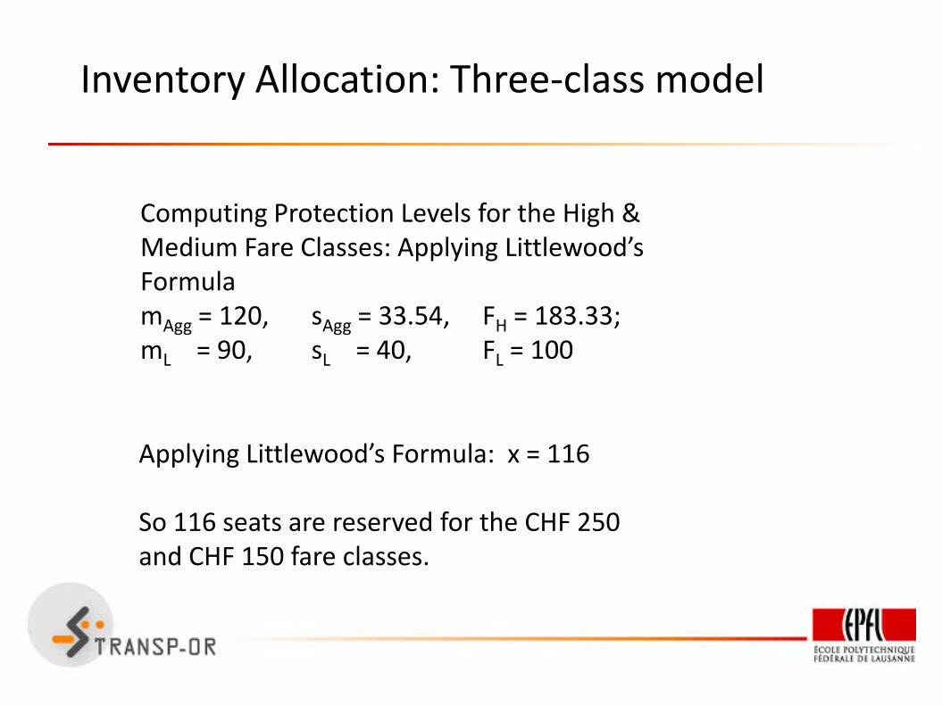
Applying Littlewood’s Formula: x = 116
So 116 seats are reserved for the CHF 250 and CHF 150 fare classes.
Computing Protection Levels for the High & Medium Fare Classes: Applying Littlewood’sFormulamAgg = 120, sAgg = 33.54, FH = 183.33; mL = 90, sL = 40, FL = 100
Inventory Allocation: Three-class model

Computing Protection Levels for the High Fare Class: Applying Littlewood’s FormulamH = 40, sH = 15, FH = 250; mM = 90, sM = 30, FL = 150.
Littlewood’s Formula:Find x such that 250 Prob(DemandH ≥ x) = 150
Inventory Allocation: Three-class model

Applying Littlewood’s Formula: x = 36
So 36 seats are reserved for the CHF 250 fare classes.
Inventory Allocation: Three-class model
Computing Protection Levels for the High Fare Class: Applying Littlewood’s FormulamH = 40, sH = 15, FH = 250; mM = 90, sM = 30, FL = 150.

120 seats
36 seatsprotected forCHF 250 class
116 seats protected for CHF 250 & CHF 150 classes
Inventory Allocation: Three-class model

Capacity: 200 Seats
Room Type
Demand
FaresMean Std. Dev.
Executive 30 10 7000
Deluxe 50 20 6000
Special 80 25 4000
Normal 150 100 2500
Inventory Allocation: Four-class model

● Consider a booking request that comes for the CHF 100 fare class
● Suppose that 25% of the people demanding bookings in the CHF 100 fare class are willing to jump to the CHF 150 fare class if necessary (up-sell probability)
● Also suppose 2 seats are already booked for the CHF 100 fare class
Inventory Allocation: Willingness to pay

If we turn her away, then
● She may pay for higher class
● She may refuse and higher class demand < 118
● She may refuse and higher class demand 118
Inventory Allocation: Willingness to pay
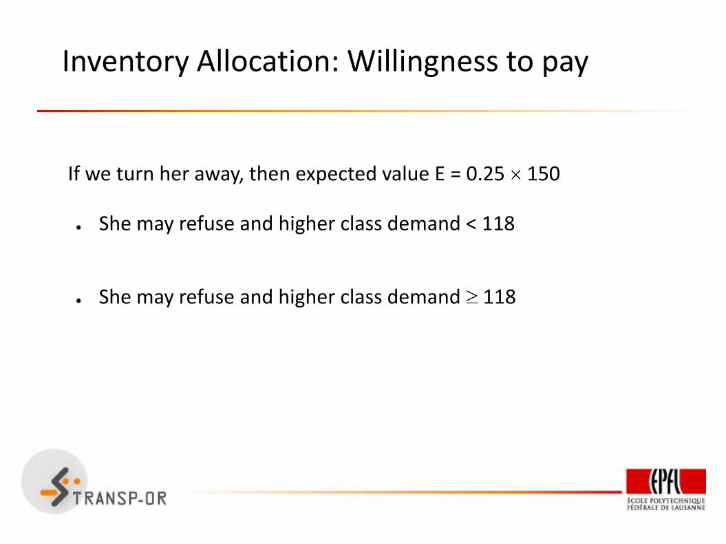
If we turn her away, then expected value E = 0.25 150
● She may refuse and higher class demand < 118
● She may refuse and higher class demand 118
Inventory Allocation: Willingness to pay

If we turn her away, then expected value E = 0.25 150+0
● She may refuse and higher class demand 118
Inventory Allocation: Willingness to pay

If we turn her away, then expected valueE = 0.25 150+0+(1-0.25) 1833.33 Prob(DemandAgg 118)
Inventory Allocation: Willingness to pay
If E > 100, then we refuse the seat at CHF 100 but remainopen for booking it at 150;
Else we book the seat at CHF 100.
Inventory Allocation: Willingness to pay

● All service industries, airlines in particular, need to manage limited capacity optimally
● Transferring capacity between compartments
● Upgrades
● Moving Curtains
● Changing aircraft capacity
● Upgrade/downgrade aircraft configuration
● Swapping aircraft
Capacity Management

69
Flight Overbooking
● Airlines overbook to compensate for pre-departure cancellationand day of departure no-shows
● Spoilage cost - incurred due to insufficient OB
● Lost revenue from empty seat which could have been filled
● Denied Boarding Cost (DBC) - incurred due to too much OB
● Cash compensation
● Travel vouchers
● Meal and accommodation costs
● Seats on other airlines
● Cost of lost goodwill

70
Capacity
ExpectedCost of Spoilage(Opportunity Lost)
ExpectedCost of Denied
Boardings
Expected Cost of Overbooking
ExpectedTotal Cost
Flight Overbooking

● Consider a fare class (with 120 seats) in a airline where booking starts 10 days in advance.
● Each day a certain (random) number of reservation requests come in.
● Each day a certain number of bookings get cancelled (cancellation fraction = 0.1).
Overbooking: Illustration

Day Bookings
1 14 14
2 -1 23 36
3 -1 -2 46 79
4 -1 -2 -5 17 88
5 -1 -2 -4 -2 50 129
6 -1 -2 -4 -2 -5 27 142
7 -1 -2 -3 -1 -5 -3 27 154
8 -1 -1 -3 -1 -4 -2 -3 33 172
9 -1 -1 -3 -1 -4 -2 -2 -3 14 169
10 -1 -1 -2 -1 -3 -2 -2 -3 -1 153
No Limits
Overbooking: Illustration

Day Bookings
1 14 14
2 -1 23 36
3 -1 -2 46 79
4 -1 -2 -5 17 88
5 -1 -2 -4 -2 41 120
6 -1 -2 -4 -2 -4 13 120
7 -1 -2 -3 -1 -4 -1 12 120
8 -1 -1 -3 -1 -3 -1 -1 11 120
9 -1 -1 -3 -1 -3 -1 -1 -1 12 120
10 -1 -1 -2 -1 -3 -1 -1 -1 -1 108
No Overbooking
Overbooking: Illustration

Day Bookings
1 14 14
2 -1 23 36
3 -1 -2 46 79
4 -1 -2 -5 17 88
5 -1 -2 -4 -2 50 129
6 -1 -2 -4 -2 -5 15 130
7 -1 -2 -3 -1 -5 -2 14 130
8 -1 -1 -3 -1 -4 -1 -1 12 130
9 -1 -1 -3 -1 -4 -1 -1 -1 13 130
10 -1 -1 -2 -1 -3 -1 -1 -1 -1 118
Overbooking 10 seats
Overbooking: Illustration

0
20
40
60
80
100
120
140
160
180
200
1 2 3 4 5 6 7 8 9 10
Bookings No Overbooking Overbooking 10 seats
Overbooking: Illustration

Cancellations
● Customers cancel independently of each other.
● Each customer has the same probability of cancelling.
● The cancellation probability depends only on the time remaining.
Overbooking: Concept

LetY : number of reservations at hand, and q : probability of showing up for each reservation.
Then the number of reservations that show up
Binomial with mean qY, and variance q(1-q)Y.
We can approximate this withNormal with mean qY, and variance q(1-q)Y.
Overbooking: Concept

Criterion – Type I service level: The probability that the demand that shows up exceeds the capacity.
qY
The demand thatshows up on theday of service.
demand
pro
bab
ility
capacity
Type I servicelevel
Overbooking: Concept

Criterion – Type I service level:
Capacity: 200 seats
Showing up probability: 0.9
Reqd. Type I service level: 0.5%
Overbooking limit?
Overbooking: Concept

Let the limit be Y.
0.9Ydemand
pro
bab
ility
200
Variance = 0.9 0.1 Y
Y turns out to be 219.
Overbooking: Concept

● Criterion – Type II service level: The fraction of customersdenied service in the long run i.e. (Expected number ofcustomers denied service / Expected number of customers )
● Criterion – Minimize Spillage and Spoilage costs
Overbooking: Concept

Capacity
OverbookingLimit
Time
Cancellation Probabilities remain constant overtime
Overbooking: Cancellation probabilities

Cancellation Probabilities decreasing withtime
Capacity
OverbookingLimit
Time
Overbooking: Cancellation Probabilities