(0 LECTESEC 211988R

U, fIo cOF

DEPARTMENT OF THE AIR FORCE

AIR UNIVERSITY

AIR FORCE INSTITUTE OF TECHNOLOG Y

Wright-Patterson Air Force Base, OhioDISTRIBUTIONI_ STATEMENT A

Dwrbuton nliite 12 20 012

AFIT/GCA/LSQ/88S-6

ESTIMATING AIRCRAFT AIRFRAME TOOLING COST:

AN ALTERNATIVE TO DAPCA III

THESIS

Patricia L. Meyer DTICCaptain, USAF

AFIT/GCA/LSCV88S-6 U E lT .ArXT/C C VSS-6DEC 2 11 988 "

H

CAs

Approved for public release; distribution unlimited

ra

The contents of the document are technically accurate, and nosensitive items, detrimental ideas, or deleterious information iscontained therein. Furthermore, the views expressed in thedocument are those of the author and do not necessarily reflectthe views of the School of Systems and Logistics, the AirUniversity, the United States Air Force, or the Department ofDefense.

AFIT/GCA/LSQ/88S-6

ESTIMATING AIRCRAFT AIRFRAME TOOLING COST:

AN ALTERNATIVE TO DAPCA III

THESIS

Presented to the Faculty of the School of Systems and Logistics

of the Air Force Institute of Technology

Air University

In Partial Fulfillment of the

Master of Science In Cost Analysis

Patricia L. Meyer, B.A.

Captain, USAF

September 1988

Approved for public release; distribution unlimited

Acknowl edgments

During the course of this research, I received substantial

assistance from several sources. I am Indebted to my thesis advisor,

Jeff Daneman, who provided continual guidance and support. My

gratitude also goes to the many people at the Aeronautical Systems

Division who provided assistance. In particular, Jim Westrich from the

Directorate of Cost, whose coments and recomnendations laid the

groundwork for the study. A special word of thanks Is due my daughter,

Farrah, for her encouragement and understanding.

Patricia L. Meyer

Acoession For

NTIS GBA&IDTIC TAB f-Unann mc e,!

,A v ,.!i r 1, .'

Dist

i i

Table of Contents

Page

Acknowledgments .......... ............. 11

Abstract ............. .......................... v

I. Introduction ...... .......................... I

Specific Problem ..... ................... 3Investigative Questions ....... ............ 3

II. Literature Review ......... ................... 4

Development of DAPCA............. . . . 4DAPCA Critique . .. .. .. .. .. .. .. .. ... 10Other Related Studies. .......... . 11Summary ...... ..................... ..... 18

III. Methodology ..... ................... ... 19

Accuracy of DAPCA III. .-. .. ......... .... 19DAPCA III Independent Variables . ........ ... 19DAPCA III Data Base . .............. .. 20Alternative Models . . . . . . . . . . . . . . .. 20Alternative to Manufacturing Factor ....... . 26

IV. Analysis . . . ........................ 27

Accuracy of DAPCA III .. ... .. .... ... 27DAPCA III Independent Variables . ........ 27DAPCA III Data Base ....... ............... 36Alternative Models .... ................ .... 36Alternative to Manufacturing Factor ... ....... 45Application Examples ........... . . .. 47

V. Conclusions/Recommendations ............... 50

Conclusions . . . . . . .............. 50Recoumendations for Further Research . . . . . . . 52

Appendix A: Comparison of DAPCA Data ............ .. 53

Appendix B: Input Data for DAPCA III ...... ............ 54

Appendix C: DAPCA III Representative Difference(without prototypes) ... .............. .... 55

Appendix D: DAPCA III Representative Difference(with prototypes) .... ................ 56

111

Page

Appendl E: CES Lot Data Information forModel Analysis .... ................. ..... 57

Appendix F: Alternative Model IndependentVariables ......... ................... 61

Appendix G: CES Lot Data Information forLearning Curves ........ ................ 6

Appendix H: Learning Curve Data ... .............. .... 65

Appendix I: Linear-Linear Model SAS Output(without prototypes) ... .............. .... 66

Appendix J: Linear-Linear Model SAS Output(with prototypes) ... ............... .... 67

Appendix K: Outlier Diagnostic Data(without prototypes) ... .............. .... 68

Appendix L: Outlier Diagnostic Data(with prototypes) ....... ............... 69

Appendix M: Alternative Model SAS Output(without prototypes) ... .............. .... 70

Appendix N: Alternative Model SAS Output(with prototypes) . .............. 71

Appendix 0: TOOL/ENGR/MFG Model SAS Output(without prototypes) ... .............. .... 72

Appenlix P: TOOL/ENGR/NFG Model SAS Output(with prototypes) ....... ............... 73

Appendix 0: CES Lot Data Information forHistorical Simulation .. ............. .... 74

Bibliography ....... ....................... . . 75

Vita .......... ............................ ..... 79

Iv

AFIT/GCA/LSW/88S-6

Abstract

The purpose of this study was to evaluate the tooling cost

estimating equation of the DAPCA III model and determine If more

accurate models can be developed. The five objectives of the research

were: (1) Determine the accuracy of the DAPCA III model. (2)

Determine If the Independent variables In DAPCA III are logically

valid. (3) Determine If the data base which was used to develop DAPCA

III Is appropriate for estimating today's aircraft systems. (4)

Determine If the accuracy of the DAPCA III model can be Improved. (5)

Determine If using a factor of manufacturing Is sufficient to estimate

tooling costs.

The study found that the accuracy of the DAPCA IiI model can be

improved by including additional variables and updating the data base.

More accurate models were developed for the data base both Including

and excluding the prototype aircraft systems.

When tooling was regressed against manufacturing and engineering,

the data without the prototypes indicated that engineering was more

significant than manufacturing. Both manufacturing and engineering

were significant for the data with the prototypes.

V

ESTIMATING AIRCRAFT AIRFRAME TOOLING COST:AN ALTERNATIVE TO DAPCA III

I. Introduction

As the United States budget deficit continues to expand, the

Government has been pressured to reduce spending. Discussions both

within and outside Congress have focused on reducing national defense

expenditures. This attention on the defense budget has stemned from the

fact that national defense expenditures have 'constituted more than

three-fifths of federal consumption expenditures and a quarter of total

government consumption expenditures (35:28).' When veteran's benefits

and space research are also considered part of the national defense

budget, 'defense and related expenditures amounted to more than

three-quarters of the federal consumption expenditures, or a third of

total government consumption expenditures (35:28)'.

With the Reagan Administration emphasis on acquiring and maintaining

a strong national defense, the defense budget has doubled in six years

(13:16). In the forecasted budget,

the Pentagon's five year plan calls for accelerated spendingon 15 new big-ticket weapons systems and putting at least 20more into production. A close look at the plan shows that newsystems and those scheduled for production during the nexthalf-decade would, if they all went forward, roughly doubledefense procurement spending over the period (13:16].

There is also growing concern that the current level of spending on

research and development will produce systems that will require large

operating and support budgets in the future. As Alexis Cain, a Defense

Budget Project Analyst, stated:

Research and development represents the acorn from whichfuture defense budgets and force postures grow. A failure toset priorities now will lead to even more difficult choices Inthe future, as the expanding defense program runs up againstthe reality of limited resources 113:35].

If Congress does not Increase defense spending or cancel new or

existing weapons procurement, the Department of Defense (DoD) will be

forced to take budget cuts from many programs (13:34-35). The Air Force

uses program cost estimates when It makes management decisions that

affect future planning and budgeting. The quality of a program cost

estimate Is determined by the quality of the estimates of the separate

program elements. Since the cost of tooling is a significant portion of

total aircraft airframe costs, It Is essential that the tooling estimates

be as reliable as possible. For example, the airframe tooling costs for

277 B-52 bombers and 316 F-15 fighters were $1309.9 million and $328.0

million, respectively (calendar year 1981 dollars) (12:B-81, B-176).

The tooling cost Is the cost to develop, acquire, and maintain the tools

necessary to produce an aircraft airframe.

Aeronautical Systems Division (ASD) cost analysts are currently

using parametric equations to estimate Air Force aircraft airframe

tooling costs for programs In the exploratory and development stages of

the acquisition cycle. Parametric models are used since program

definition Is normally vague during these stages. One parametric model

often used within ASD Is the Development and Procurement Costs of

Aircraft (DAPCA) III model, which was developed by the Rand Corporation

2

in the 1960s and 1970s (7:15). Another technique, which Is used at ASD,

Is to determine tooling costs based on a factor of manufacturing costs

(37).

The challenge to cost analysts concerned with military hardwareIs to project from the known to the unknown, to use experienceon existing equipment to predict the cost of next-generationmissiles, aircraft, and space vehicles [2:1].

Specific Problem

Determine some more accurate parametric models to estimate the cost

of aircraft airframe tooling on new Air Force aircraft systems.

Investiaative Questions

1. Is the Rand parametric model, DAPCA III, an accurate model for

estimating aircraft airframe tooling costs for new aircraft systems?

2. Are the independent variables in DAPCA III logically valid?

3. Is the data base which was used to develop DAPCA III appropriate

for today's aircraft systems?

4. Can the accuracy of the DAPCA III model be improved?

5. Is the alternative technique using manufacturing costs as the

basis to estimate tooling costs sufficiently accurate?

3

II. Literature Review

Development of DAPCA

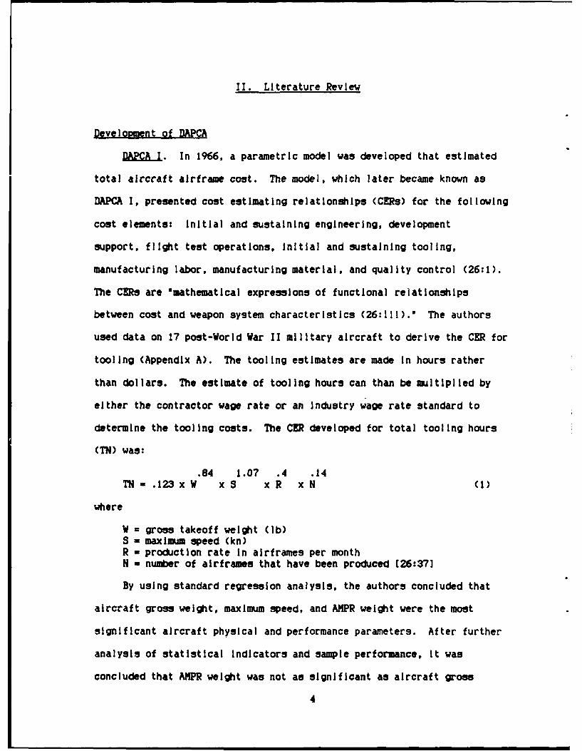
DMPKA I. In 1966, a parametric model was developed that estimated

total aircraft airframe cost. The model, which later became known as

DAPCA I, presented cost estimating relationships (CERs) for the following

cost elements Initial and sustaining engineering, development

support, flight test operations, Initial and sustaining tooling,

manufacturing labor, manufacturing material, and quality control (26:1).

The CEMs are *mathematical expressions of functional relationships

between cost and weapon system characteristics (26:111)., The authors

used data on 17 post-World War II military aircraft to derive the CER for

tooling (Appendix A). The tooling estimates are made In hours rather

than dollars. The estimate of tooling hours can than be multiplied by

either the contractor wage rate or an Industry wage rate standard to

determine the tooling costs. The CER developed for total tooling hours

(TN) was:

.84 1.07 .4 .14TN = .123 x W x S x R x N (1)

where

W = gross takeoff weight (ib)S - maximum speed (kn)R - production rate In airframes per monthN - number of airframes that have been produced (26:37]

By using standard regression analysis, the authors concluded that

aircraft gross weight, maximum speed, and ANPR weight were the most

significant aircraft physical and performance parameters. After further

analysis of statistical Indicators and sample performance, It was

concluded that AMPR weight was not as significant as aircraft gross

4

weight; therefore, AMPR weight was not Included in the final model

(26:35). The aircraft gross weight was Included to capture the variation

in tooling hours due to the size of the airframe.

The Aeronautical Manufacturers' Plannina Report's definition of

AMPR weight is

the empty weight of the airplane less (1) wheels, brakes,tires, and tubes, (2) engines, (3) starter, (4) cooling fluid,(5) rubber or nylon fuel cells, (6) Instruments, (7) batteriesand electrical power supply and conversion equipment, (8)electronic equipment, (9) turret mechanism and power operatedgun mounts, (10) remote fire mechanism and sighting andscanning equipment, (11) air conditioning units and fluid, (12)auxiliary power plant unit and (13) trapped fuel oil 126:5].

Speed Is used as an Index of the structural design features of the

aircraft. For example, airframes flow at higher speeds require *the use

of higher cost and more difficult to work with materials, e.g., titanium,

stainless steel and honeycomb sandwich structures (8:32).' This type of

material Is needed for an airframe *to withstand the heat generated by

atmosphere at a speed of about Mach 3. . . (2:88).0

The exponent for the variable N used in equations I and 3 represents

the hours versus quantity relationship (learning curve slope) (26:26).

This learning effect Is the decrease In recurring tooling costs as more

units are produced. The slope of .14 was determined by finding the mean

of the cumulative tooling hour slopes of 11 of the aircraft In the

sample. To determine the cumulative tooling hour slope for each

aircraft, the authors plotted the cumulative tooling hours versus the

cumulative number of airframes produced on log-log grids. The slope was

measured by visually fitting a straight line through the points. The

authors reduced possible distortions in the data by using a production

Interval for each aircraft during which the production rate did not

change and no major modifications occurred (26:26).

5

An adjustment factor for the rate of production (R) was Included

since the authors felt there was a 'direct relationship between the rate

at which airframes are manufactured and the physical volume of production

tools that is required (26:25).' In determining the adjustment factor

of R with an exponent of .4, the authors were limited to using

observations on five fighter aircraft due to limited production rate

data. For each aircraft system, two points, which had differing

production rates, were picked on the cumulative tooling hour plot. A

line was drawn using the slope of .14 to determine the respective

Intercept (tooling hour) values for each point. Using the Intercept

values and production rates of the two lines, the ratio of production

rates and ratio of tooling hours were calculated and plotted for each

system. An analysis of the 'apparent best fit' led the authors to

conclude that a factor of R with an exponent of .4 should be used to

adjust the tooling hour estimates for changes in production rates

(26:29).

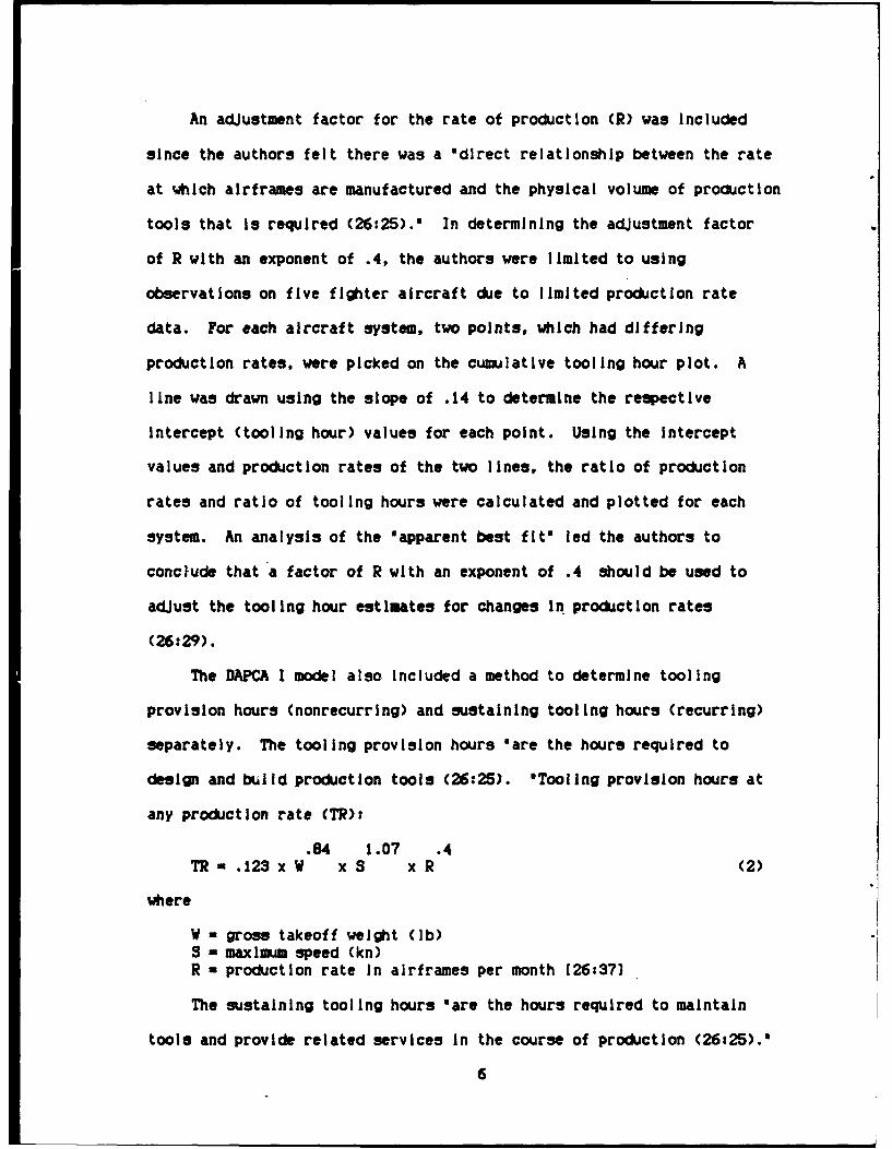
The DAPCA I model also Included a method to determine tooling

provision hours (nonrecurring) and sustaining tooling hours (recurring)

separately. The tooling provision hours $are the hours required to

design and build production tools (26:25). 'Tooling provision hours at

any production rate (TR):

.84 1.07 .4TR .123 x W x S x R (2)

where

W = gross takeoff weight (ib)S - maximum speed (kn)R - production rate in airframes per month (26:37]

The sustaining tooling hours 'are the hours required to maintain

tools and provide related services in the course of production (26:25).'

6

Sustaining tooling hours (TS):

.14TS = TN - TR = TR(N - 1) (3)

where

TN - total tooling hoursTR = tooling provision hours at any production rate

N - number of airframes that have been produced [26:37]

DAPCA II. The Rand Corporation updated the DAPCA I model In 1972.

The new model, DAPCA 1I, was based on a revision of the DAPCA I data

base. The new tooling CER was developed using data on 29 aircraft

systems (Appendix A). Using regression analysis, the authors found ANPR

weight, maximum speed, quantity, and production rate were the most

significant explanatory variables to estimate tooling hours (27:15).

The CER developed to estimate total tooling hours (T) was:

.764 .899 .178 .066T = 4.0127 x A x S x a x R (4)

where

A - AMPR weight (Ib)S - maxilmm speed (kn) at best altitude0 - cumulative quantity including flight test

airframesR - production rate, deliveries per month [27:15]

The major differences between DAPCA I and II are due to the updated

data base, the change from gross takeoff weight to AMPR weight, and no

differentiation between recurring and nonrecurring tooling hours.

Dropping the gross weight eliminated the problem of defining gross weight

consistently. Gross weight varies based on mission requirements. "Gross

take-off weight is a function of the amount of avionics installed, type

and amount of armament, and fuel load (4:27).' AMPR weight was used to

indicate the relationship between the size of the aircraft and tooling

hours (27:15).

7

DAPCA II does not provide separate estimates for nonrecurring and

recurring tooling, since *definitional inconsistencies among contractors

made the distinction meaningless (23:11).

Another major change was the way the learning curve effect was

incorporated Into the model. Quantity was included as one of the

independent variables when regression analysis was used to develop the

CER. The exponent for the quantity variable indicates a measure of the

learning curve slope. Production rate was also used as an independent

variable. The methodology used In DAPCA I to calculate a production rate

adjustment factor was not used in DAPCA II because of data limitations

(27:15-16).

A later study by the Rand Corporation addressed the 'degree of

confidence that can be placed In cost predictions for airframes obtained

from' DAPCA II (36:1). The authors determined prediction Intervals for

five design points with weight and speed values that generally bound the

aircraft In the sample. 'Prediction Intervals are limits within which,

with a specified probability, the value of a single future observation

lies (36:2).'

The study revealed wide prediction Intervals for total aircraft

airframe costs using DAPCA II. At a 95 percent confidence level, 'the

actual cost will lie some where between a 43 percent underrun and a 75

percent overrun (36:30).' The authors emphasized that when a parametric

model is used to establish cost figures for a system acquisition, the

width of the prediction Interval Is extremely important. Since the

analysis of the prediction intervals in the study were for total aircraft

airframe costs, the prediction intervals for total tooling hours Is

8

unknown. However, the study implies that DAPCA II tooling estimates may

have wide prediction intervals.

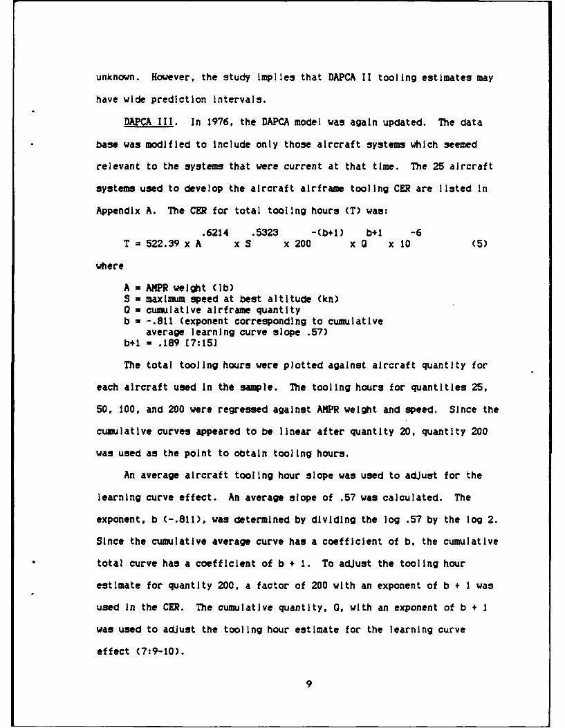
DAPCA III. In 1976, the DAPCA model was again updated. The data

base was modified to include only those aircraft systems which seemed

relevant to the systems that were current at that time. The 25 aircraft

systems used to develop the aircraft airframe tooling CER are listed in

Appendix A. The CER for total tooling hours (T) was:

.6214 .5323 -(b+l) b+l -6T = 522.39 x A x S x 200 x Q x 10 (5)

where

A = AMPR weight (ib)S - maximum speed at best altitude (kn)0 - cumulative airframe quantityb = -.811 (exponent corresponding to cumulative

average learning curve slope .57)b+1 = .189 (7:15]

The total tooling hours were plotted against aircraft quantity for

each aircraft used in the sample. The tooling hours for quantities 25,

50, 100, and 200 were regressed against AMPR weight and speed. Since the

cumulative curves appeared to be linear after quantity 20, quantity 200

was used as the point to obtain tooling hours.

An average aircraft tooling hour slope was used to adjust for the

learning curve effect. An average slope of .57 was calculated. The

exponent, b (-.811), was determined by dividing the log .57 by the log 2.

Since the cumulative average curve has a coefficient of b, the cumulative

total curve has a coefficient of b + 1. To adjust the tooling hour

estimate for quantity 200, a factor of 200 with an exponent of b + I was

used In the CER. The cumulative quantity, 0, with an exponent of b + 1

was used to adjust the tooling hour estimate for the learning curve

effect (7:9-10).

9

Boren found that Including a production rate variable did not reduce

the residuals and was not significantly statistically (23:12).

Therefore, the DAPCA III model did not Include a production rate

variable.

Since there were significant average deviations from the regression

line for small quantities, the total tooling estimate was adjusted for

quantities less than 20:

.699

T (adjusted) - T x .1232 x 0 [7:153 (6)

The adjustment factors were calculated by assuming that a quantity of 20

units will have tooling cost five times that of a quantity of two units.

The derivatives of a and b proceeds as follows:

b1.00 a x 20 (7)

b.20 a x 2

b

5 - 10

Solving for the unknowns, Boren determined that b - .6990 and a , .1232.

Boren emphasized that this approach for adjusting for smaller quantities

provides a rough approximation. He recomnends that DAPCA III not be used

on programs that have a very small production quantity.

DAPCA Critioue

A 1977 Rand study evaluated several parametric models available to

estimate aircraft airframe costs. The authors concluded that 'parametric

cost models requiring only a few aircraft characteristics as Inputs can

provide useful estimates of airframe cost (23:47)." However, the

authors were concerned that the models In some Instances *also produce

estimates that may be off-target by over 100 percent (23:47).6 To

10

Improve future models, the following recommendations were made:

a. Provide a way to distinguish between Air Force and Navy aircraft

program costs.

b. Determine an objective procedure to measure technological

change.

c. Use dummy variables to distinguish between types of aircraft:

cargo, bomber, and fighter.

d. Investigate contractor variables (23:48).

An evolution of parametric cost models was presented In a 1981 Rand

study. The study pointed out that:

Physical and performance factors such as weight and speed arenot sufficient In themselves to deal with next generationaircraft, but some Judgmental factors are too unreliable toinclude in a parametric cost model (22:20].

The tooling costs estimated by DAPCA III are based on weight and

speed. Therefore, there Is reason to doubt that DAPCA III is the most

valid parametric model for estimating the cost of aircraft airframe

tooling on new Air Force aircraft systems.

Other Related Studies

The following review of several studies on aircraft airframe cost

estimating will provide Insight Into potential cost relationships and

modeling techniques.

In April 1967, The Planning Research Corporation (PRC) published an

airframe model which consisted of separate estimating equations for

several cost elements at production units 10, 30, 100, and 300.

Cost-quantity curves were derived from these estimates (3:10). Since

high performance aircraft have a high proportion of nonrecurring cost and

therefore extremely steep slopes, PRC felt the cost curves for

11

engineering and tooling might not be linear. It was determined that the

CERs for engineering and tooling would be more feasible If recurring

and nonrecurring costs were separated (33:1-3, 11-7). When PRC tried to

separate these costs, variability was introduced which was not explained

by the CER. PRC found that by combining the engineering and tooling

costs and developing CE s for nonrecurring and recurring costs, the

variability could be significantly reduced (33:1-4).

The nonrecurring tooling and engineering CER had two Independent

variables:

a. the ratio: (empty weight minus airframe unit weight) divided by

airframe unit weigt.

b. maximum speed at altitude in Mach number.

The independent variables in the recurring tooling and

engineering CER were:

a. the ratio: (empty weight minus airframe unit weight) divided by

airframe unit weight.

b. maximum speed at altitude in Mach number.

c. percent change In airframe weight from unit one at the nth

production unit.

d. calendar year of first delivery minus 1940 (33:111-17, 20, 21).

The time variable was 'used to express the effect of time-related

factors, such as changes In the technological state-of-the-art

(33:11-2)."

The PRC model requires inputs that are 'not available until a

production schedule has been laid out and a contractor chosen (23:19).,

Therefore, it cannot be used to estimate programs early in the

12

acquisition cycle. Also, since the estimates for tooling and engineering

are combined, estimates for tooling costs are not available.

J. Watson Noah Associates, Inc. developed CERs In 1973 for recurring

and nonrecurring total aircraft airframe costs. The authors estimated

cumulative cost-per-pound of ANPR weight at quantity 100, and then

applied a learning curve with an 80 percent slope (29:56).

The Independent variable used In the nonrecurring total

airframe CER were:

a. maximum speed at best altitude.

b. gross take-off weight divided by ANPR weight.

c. complexity Indicator variable.

d. technological index.

The recurring total airframe CER had the following

Independent variables:

a. maximum speed at best altitude.

b. AMPR weight.

c. complexity Indicator variable.

d. technological index (29:50).

The complexity indicator variable, which is based purely on a

Judgment call, was used to capture differences in complexity. The

authors found four aircraft whose costs were seriously underestimated.

'Each had a major mission or performance parameter which required

significantly new and complex technology (29:48).'

The authors felt that an appropriate measure of technology should be

$constructed on the basis of the model changes that have occurred over an

appropriate period of time (29:29).' Therefore, the technology progress

13

Index was based on the 'number of model changes that have occurred since

aviation progress began to accelerate during World War I (23:29).'

In 1977, J. Watson Noah Associates, Inc. revised their 1973 model.

The 1977 model consisted of two CERs. One estimated the total aircraft

airframe costs for design. The other estimated the total aircraft

airframe costs for production. Both recurring and nonrecurring tooling

costs are Included In the production CER (23:34). The authors also used

a log-linear form In the 1977 model, while the 1973 model used an

arithmetic functional form (4:17) Again, the tooling cost estimates are

not available since the CERs estimated total aircraft airframe costs.

The Rand Corporation performed a study In 1976 to determine If there

were characteristics In addition to weight and speed (the Independent

variables in DAPCA III) 'that would make an estimating model more

flexible and hence better able to deal with characteristics peculiar to

Individual aircraft (24rv). The authors developed a total aircraft

airframe model. The CER estimated the total cost for 100 units as a

function of airframe unit weight and maximum speed (24:42). All attempts

to Increase the reliability of the estimates by using additional

Independent variables were not productive (24:53).

In 1977, the Rand Corporation developed a fighter aircraft

estimating model. The data, which was from the DAPCA III data base,

included attack and fighter aircraft, plus B-58, T-38, F-84, F-86A, F-89,

F-3D, and F-101. The authors developed a model specifically to estimate

fighter aircraft airframe costs, since they felt that such a model would

provide a better estimate of fighter aircraft cost than from a model

14

derived from a sample Including the KC-135 tanker and the C-5 cargo

aircraft (21:1). The independent variables In the model were:

a. airframe unit weight.

b. maximum speed.

c. gross take-off weight divided by airframe unit weight.

d. specific power, which equals:

(static thrust) x (max speed)combat weight x (.003069) (8)

(21:2, 6]

This model also calculated total airframe costs, so an estimate of

only tooling cost Is not be available. The estimates from the

all-fighter sample model were compared to estimates from a broader-based

model. The authors found 'that when estimating total cost it makes

little difference which of the models Is used (21:14).' Although

the authors were not able to show a fighter model was better than a

broader-based model, this does not mean it could not be true.

The Modular Life Cycle Cost Model (MLCCM) was developed by the

Grumman Aerospace Corporation In 1976 and later updated In 1980. The

model estimates airframe, engine, and avionics costs In the Research,

Development, Test, and Evaluation (RDT&E), Production and Operation and

Support (0&S, phases. MLCCH Is comprised of CERs which 'were developed

to conform to a work breakdown structure format to provide visibility to

the subsystems In each design (19:30).' The independent variables for

the total tooling labor manhours were:

a. the number of prototype aircraft In first buy.

b. ultimate load factor, which Is the amount of 'g' forces the

aircraft can sustain.

c. maximum Mach number.

15

d. total wetted area, which Is a measure of aircraft volume (3:20).

The NLCCM model uses an index to adjust the cost of all-aluminum

airframe estimates for differences in the amount of composite materials.

The cost factors are developed for each of the main sections of an

aircraft, wing, fuselage/nacelle, and tall (19:32).

Clemson University performed a series of studies In the late 1970's

and early 1960's to determine an econometric model to estimate the cost

of military aircraft airframes. 'An econometric model Is a system of

Interdependent equations that describe some real phenomenon . . . These

equations are solved simultaneously to find the values for unknown

variables . . . (9:273).' The Clemson model determines the cost to

produce an individual aircraft based on its start date and Its planned

delivery date. Another feature of the model are four production cost

drivers: " learning by doing, learning over time, the speed of the

production line, and production line length (40:iv).0 The equations In

the model Incorporate the technical features of the airframe production

program and the contractor's behavior (40:iv).

The model has the advantage of providing decision makers with the

effects of alternative schedules (40:226). The authors note that

the model 'requires considerable knowledge of both the planning and

production stages in any airframe program (40:2).' This Information Is

not available In the early stages of planning. Also, the model does not

provide a breakout of costs by cost element, so the cost of tooling is

not attainable.

In 1982, the Air Force Institute of Technology sponsored a thesis to

determine If there was Justification to support the development of

separate cost equations for the airframes of fighters, attack, and cargo

16

aircraft. A statistical procedure, factor analysis, was performed on

performance characteristics of the aircraft airframes. The authors

concluded that the factor analysis Justified separating the airframe cost

data by fighter, attack, and cargo aircraft and developing a separate CER

for each group (3:86).

A thesis on estimating the cost of composite material airframes was

completed at the Air Force Institute of Technology In 1983. The author

developed an Index of adjustment factors that reflect the differences

between aluminum and composite material airframe costs for nonrecurring

tooling manhours, recurring manufacturing manhours, and material dollar

costs. The tooling costs were estimated by comparing tooling hours

generated by the ICAM Manufacturing Cost/Design Guide to set up hours

used In the Fabrication Cost Estimating Technique (FACET)(19:41,42).

There Is a potential problem, since the tooling costs captured by the two

models are not Identical. The author warns that *uncertainties In the

exact relationship between the tooling cost captured in FACET and the

tooling costs captured In the ICAM manual must be resolved before the

Index can be used (19:93).

An aircraft airframe cost model, which has adjustment factors to

account for changes In technology and variations In the material

composition of the airframe, was developed by the Aeronautical Systems

Division In 1984. The DAPCA III CERs are used In the model. An

equivalent metals weight factor Is determined based on the percentages of

each type of material In the airframe. The weight Independent variable

to be used In the DAPCA III model Is adjusted using this weight factor

(6:8-11). An estimate of the tooling costs Is calculated using DAPCA

17

III. This estimate is then adJusted using a technology factor, which Is

determined by the Judgment of experts.

Summary

There have been several models developed to estimate the cost of

aircraft airframe tooling. The DAPCA III model is often used at the

Aeronautical Systems Division. The purpose of this study will be to

evaluate the accuracy of the tooling cost estimating equation in DAPCA

III and determine If models can be developed that are more accurate than

the DAPCA III.

18

III. Methodoloay

Accuracy of DAPCA III

To determine whether the DAPCA III model is an accurate estimator of

aircraft airframe tooling cost estimates, DAPCA III will be tested using

actual aircraft specifications from the Air Force Cost Center's Cost

Estimating System (CES)(IO:4-1 thru 4-923). These specifications will

be used in Eq (5) to determine a DAPCA III estimate. The aircraft

systems used for this test will be the systems used by Rand to develop

DAPCA III. The estimates derived from running the model will be compared

to actual tooling costs in the CES. To determin 'he representative

difference between the actual costs and the estimated costs the following

formula will be used:

[5 2representative difference - (actual-ftimate)" (9)

V number of observations

The representative difference will be calculated for the data base

without prototypes and with prototypes. The representative difference is

used to determine the accuracy of DAPCA III, since it can be compared to

the coefficient of variation or root mean square of the models which will

be developed during this research.

DAPCA III Independent Variables

An analysis of previous studies will provide Insight Into whether

the Independent variables used in DAPCA III are logical. Each

Independent variable will be discussed and a conclusion made whether it

it Is still a logical variable for estimating costs of future aircraft

systems.

19

DAP A III Data Base

The aircraft systems In the CES will be reviewed to determine which

aircraft systems provide the best representative sample of future

aircraft systems. The data base used to develop DAPCA III will be

compared to the aircraft systems Identified In the CES.

Alternative Models

Considering the results of the analysis of Independent variables and

the data base, a model which estimates aircraft airframe tooling cost on

new Air Force aircraft systems will be developed. To Identify the

Independent variables for the model, the systems attributes that are

felt to have an effect on the cost of tooling will be determined.

Then the aircraft physical and performance characteristics that reflect

those system attributes will be identified. These characteristics will

then be considered as potential Indepindent variables.' Possible

Indicator variables and Interaction effects will also be considered. The

Indicator variables, which are also known as dummy variables, will be

used as a way of Oquantitatively Identifying the classes of a qualitative

variable (28:329).' Interaction effects on the dependent variable Y

occur when, given independent variables XI and X2, "both the effect of XI

for a given level of X2 and the effect of X2 for a given level of XI

depends on the level of the other independent variable (28:232).'

After the potential Independent variables are Identified, the Impact

each variable has on tooling costs will be specified. For example, If

weight Is chosen as an independent variable, It would be specified

whether an Increase In weight would be expected to increase or decrease

the cost of tooling.

20

All analyses to determine an alternative model to DAPCA III will be

performed on two separate data bases. One data base will Include data on

the prototype aircraft systems. The other data base will eliminate the

data on the prototype aircraft systems. This procedure will provide

Information on the Impact of the developmental aircraft systems on the

total cost of tooling. The criteria to identify the prototype aircraft

In the data base will be:

a. Identify any aircraft which have a prototype model designator.

For example, the A4D-1 prototype was designated XA4D-I.

b. If the number of prototypes Is known and the first lot of an

aircraft is that number, assume the first lot contains the prototype

data.

c. If first lot Is large, assume prototype data is Included as part

of the first lot.

Since the cost of direct labor varies between contractors, the

dependent variable In the models will be in direct labor hours Instead of

dollars.

The method to capture the learning curve effect will be similar to

the method used in DAPCA III. The major difference will be the dependent

variable which will be the cumulative average tooling hours through unit

100, while DAPCA III used the cumulative average tooling hours through

unit 200. By using only the first 100 aircraft, possible distortions due

to major modifications are minimized. The cumulative average tooling

hours through unit 100 for each system will be calculated by using the

following formula:

21

CA = A x 100 (10)

100

where

CA = cumulative average tooling hours for units I through 100100A - first unit cost (hours)b - rate of learning (20:18)

To determine the rate of learning and the first unit cost (hours)

the lot data in the CES report will be used in the cumulative average

learning curve software program developed by Hutchison In 1985

(18:26-69). The median of the learning curve slopes for each data set

will be used as the average learning curve slope for that data set. The

learning curve slope in DAPCA III was determined using the arithmetic

mean. The median is a better measure of the average learning curve slope

than the arithmetic mean, since it does not distort the average when the

data Is skewed to the left or right. Also, an abnormal learning curve

(e.g. a positive slope) would not raise the median slope as much as it

would raise the arithmetic mean slope.

The cumulative average tooling hours through unit 100 will be

regressed against the independent variables using the statistical package

on the SAS program (34:113-137, 655-709). The data will be regressed in

both linear and log-linear forms to determine which formulation has a

lower predicting error. The data will also be regressed with and without

inclusion of the prototypes In the data set, to determine If there is a

difference In predicting tooling hourss dependent on the stage of

development.

Initially, the data will be regressed using a multiplicative

relationship, where Y Is A times X to the B power. This relationship

limplIe, a deceleration or an acceleration in cost depending on the

22

values of the coefficients of the logarithmic terms (15:4).' The

logarithm-linear (multiplicative) form has been *used by Rand because of

the Implied diminishing marginal returns when coefficients are less than

1.0.(4:14).' DAPCA III is in logarithm-linear form. Rand found this

form to fit the data best.

The multiplicative form must be changed to a linear form so that

regressions calculations can be performed. The transformation will be

done by taking the natural logarithms of both sides of the equation

(inY - InA + BInX + Ine).

The data will also be regressed using a standard-linear relationship

(Y - A + BX + e). This linear form Implies a constant relationship

between the dependent and Independent variables (15:4). The results of

the linear model will be compared to the results of the logarithm-linear

model to determine which form fits the data best.

To determine whether the model Is linear or log-linear, the models

for the data both with and without the prototypes will be evaluated using

the following criteria:

a. Calculated F-ratio greater the critical F-value at a 90 percent

confidence level. If the F test statistic Is significant, then there is

a relationship between the dependent variable and the set of Independent

variables (28:289).

b. Calculated t-statistic greater than the critical t-statistic at

an 85 percent confidence level for each Independent variable in the

model. If the t statistic Is significant, then the amount of variation

In the dependent variable that Is explained by the Independent variable

Is significant (28:289).

c. For linear models, a low coefficient of variation (11:54).

23

d. For log-linear models, a low root mean square error(11:7).

e. For the logarithm-linear form, If the parameter estimate

(coefficient) Is greater than 1.0, then as X Increases, Y Increases more

than proportionally (exponentially), which means the Independent variable

Is questionable In this relationship.

The models that appear to have the best fit will be analyzed for

potential outlying observations In the data set. To determine if any

observations are extreme with respect to X, the leverage values will be

reviewed. The leverage value Is the measure of the distance between the

X values for a specific observation and the means of the X values for

all observations In the data set (28:402). A leverage value greater

than 2p/n, where p = number of parameters and n = number of observations,

will Indicate outlying observations with respect to X (28:403).

The studentlzed deleted residuals will be reviewed to determine If

any of the observations in the data set are outlying with respect to Y

(28:404). If the studentized residual Is greater than the t-value at

a confidence level of 90 percent, they will be considered outlying

observations with respect to Y.

The Cook's distance measure will be used to determine the Impact of

each observation on the estimated regression coefficients (28:407).

If the Cook's d for an observation Is greater than an F-value at 50

percent, that observation will be considered an influential observation.

The learning curve effect will be integrated Into the models that

are selected. Since the models will estimate the cumulative average

tooling hours of the first 100 aircraft, an adjustment for varying

quantities of aircraft and the learning effect must be made. If the

models are logarithm-linear, the following adjustments will be made:

24

If selected model is Y = AX(exp bl), then adjusted model will be:

bl (b2 + 1) -(b2 + 1)Y = A x X x 0 x 100 (11)

whereY a cumulative average tooling hoursA - InterceptX - Independent variablebl - coefficient of Independent variable0 - quantityb2 - average learning curve

This methodology Is analogous to that used for DAPCA III, Eq (5). If the

models are standard-linear, the following adjustments must be made by the

the user of the model:

If selected model Is Y - A + bIX, then using the average learning

curve slope and the cumulative average hours of the first 100 airframes

determine the cost of airframe one. Use the estimate of the first unit

hours (A) in the following formula:

bY -AX (12)x

where

Y - cumulative average tooling hours of first X airframesxA - first unit cost (hours)X - cumulative number of airframesb - rate of learning

The cumulative average number of hours Is the multip lied by the number of

airframes to determine the total cumulative hours.

The coefficient of variation/root mean square for each of the models

selected will be compared to the value of the representative difference

for the DAPCA III model. This comparison will identify which model Is

more accurate based on the results of the analysis.

25

Alternative to Manufacturina Factor

The total cumulative tooling hours of the aircraft systems used to

develop the cumulative average tooling hours In the previous section

will be regressed against.the engineering and manufacturing total

cumulative hours to determine If there is a relationship between tooling

and engineering or manufacturing hours. A model will be developed for

the data base with prototypes and without prototypes. To determine If

this relationship also existed In the past, a historical simulation will

be performed. With historical simulation the data for most recent

aircraft systems are removed from the data base and then regression

analysis Is performed on the reduced sample. The estimates from the

reduced-sample model are compared to the actual data (5:55). If the data

base has a small number of observations, an equivalent number of older

aircraft systems will be added to the data base when the most current

systems are removed.

26

IV. Analysis

Accuracy of DAPCA III

The Inputs for the DAPCA III model were obtained from the Air

Force Cost Center's CES (Appendix B). Two data points were not

available In the CBS. The first, the B-52 ANPR weight, was taken from

the Rand report on DAPCA I (26:7). The second, the C-130 ANPR weigt,

was obtained from Information In the Lockheed Aircraft Corporation

Report ER 2342 (31:7-12).

The tooling estimates from DAPCA III were compared to the actual

tooling hours reported In the CES. The representative difference for

the data without prototypes was the square root of (679,165,399.3

hours/25) or 5212.16 hours (Appendix C). The average tooling hours

were 210,176 hours/25 or 8407.04 hours. Therefore, the representative

difference percentage was 5212.16/8407.04 or 62.00 percent. The

representative difference for the data Including the prototypes was the

square root of (669,863,341.6/25) or 5176.34 (Appendix D). The

average tooling hours were 236,909 hours/25 or 9476.36. Therefore, the

representative difference percentage was 5176.34/9476.36 or 54.62

percent.

DAPCA III Independent Variables

Size. DAPCA III uses airframe unit weight to explain the

variability due to the size of the airframe. Weight Is Oa logical

variable because It Is an Index of size, and all other things being

equal a large aircraft should cost more than a small one

(24:12).' The airframe unit weight was also found to be a significant

variable In the Noah, 1976 Rand, and 1977 Rand Fighter models.

27

Gross takeoff weight and the ratio of gross takeoff weight to

airframe unit weight have been considered as possible independent

variables In some models. Large warned there Is a problem with

•achieving a consistent definition of gross takeoff weight (24:24).'

As Bennett explained,

gross take-off weight is a function of the amount of avionicsinstalled, type and amount of armament, and fuel load. Thisresults in different values of gross weight depending uponthe mission requirements for which it Is defined [4:27].

With this In mind, gross takeoff weight should not be used to capture

the Impact of size on cost.

The PRC model used the ratio (R) of empty weight minus airframe

unit weight to airframe unit weight. Large cautioned that 'R is only a

proxy for weight and not a good one. Two aircraft with much the same

empty weight . . . can have very different Re. . . (23:21-22).'

Carrier emphasized that when using a weight-cost

relationship

for estimating purposes it is Important to make sure theconstruction and materials of the airframe to be estimatedare similar to those of the airframes on which the costestimating relationship Is based [8:31.

There has been a growing concern that the increased use of composites

in aircraft airframes will make estimating with the existing data base

questionable. The data consists of primarily aluminum aircraft

airframes. 'There are less than 10 aircraft In the inventory with

significant quantities of composite materials (19:5).' In most of

these aircraft the composite material is less than 15 percent of the

airframe weight. 'Using regression analysis of a data set with Just

these aircraft in It to make cost predictions about composite airframes

28

would not provide results that could be used with any degree of

confidence (19:5).'

This same concern impacts the estimates of airframes which

are partly composed of steel and/or titanium. 'Titanium is much

more expensive than aluminum and is more difficult to fabricate

(24:3).'

Today's airframe cost estimates must adress the issue of

variations in structural materials to ensure reliable estimates. Since

regression analysis Is not an appropriate technique, the application of

an adjustment factor, such as the one developed by ASD, seems the best

approach.

Although e..r-'.je area was not used In the DAPCA III model, It

seems to be d logical independent variable. A variable such as

airfram', surface area or wing area should capture the variations

in size.

While weight has explained the variations In cost due to size, it

does not capture the cost variability caused by performance

differences. As Carrier explained,

The weight and general purpose of two items, for example,might be exactly the same, yet the performance of one, gainedthrough advancement in design, materials, and fabricationtechniques, might be considerably better than that of theother. The possibility exists, therefore, that the improvedItem might cost considerably more, and If Its cost Isestimated on the basis of weight alone It might beunderestimated by a large amount 18:3,5).

frmance One performance characteristic that tends to vary

with tooling costs is speed. The DAPCA III, PRC, Noah, 1976 Rand, 1977

Rand Fighter, and MLCCM models all used speed as an independent

variable. Large cautions that 'other organizations have found It to be

of no significance (24:12).'

29

DAPCA III does not Include any independent variables that would

capture the variations in maneuverability of the aircraft systems.

Variations in maneuverability would change the degree of stress on the

airframe and could vary the structural and tooling requirements. Two

characteristics which logically represent the aircraft's

maneuverability are the thrust-to-welght ratio and the rate of climb.

Since climb rate is based on gross takeoff weight it should not

be used for the reasons mentioned earlier.

Production Rate. DAPCA III does not consider changes in the

production rate. The authors of DAPCA I believed that there 'is

an obvious direct relationship between the rate at which airframes

are manufactured and the physical volume of production tools that

is required (26:25).' Carrier also felt production rate impacts

tooling costs. He stated that 'the expected number of components

to be produced helps determine the production rate which In turn

has an effect on tooling costs and on production costs through the

amount and type of tooling . . . (8:3).' He further explained,

An extremely low production rate Is held to be inefficientbecause of under-utilization of facilities. Up to a certainpoint output can be Increased without a proportional Increasein the cost of management, tooling and facilities. Beyondthat point these costs increase more rapidly than output,offsetting the economies of scale secured in other aspects ofproduction (8:563.

Dreyfuss also agrees that some tooling Is time-

dependent:

an initial set of tools is fabricated to supportmanufacturing at some specified maximum rate of production(e.g., four aircraft per month). Recurring or sustainingtooling has a fixed component that is time-dependent and avariable component that is a function of quality. The formerwill Increase as program length Increases; the latter Islargely unaffected by production rate (14:83.

30

However, he also explains that it Is difficult Is not Impossible to

Isolate the portion that is time-dependent. He concludes that 'within

the limits of the rates examined production rate has little effect on

tooling hours (14:39).'

In 1974, the Rand Corporation published a relatively toorough

study, which analyzed 'the effect of production rate on the cost of

selected types of military hardware (25:v).6 The authors concluded

that their analyses 'suggest but do not confirm that cumulative tooling

cost Is not highly sensitive to the rate of output (25:20).' They

explained:

In general it appears that an increase In production rateshould result in a decrease In such costs, but In anyspecific case the effect depends on how rate changes areachieved, the availability of suppliers, the local laborsupply, management policy, the timing of rate changes, plantcapacity, plant backlog, and a number of other factors(25:v].

In 1980, Womer noted that the Rand reports on aircraft cost, which

'have been cross-sectional studies characterized by a few observations

on many aircraft programs,' credit 'production rate with little, If any

explanatory ability (39:2).' He also noted that some time series

studies on single airframe programs *indicate that production rate Is

correlated with costs on a program (39:2).0 There does not seem to

be any consistent relationship between production rate and tooling

costs. Womer reported there are 'documented cases where increases in

production rate have been associated with increases, decreases, and no

change In the unit cost of production (39:1)'.

Since production rate is hard to predict In advance, may be

subject to change, and Its affects are dependent on how the rate is

31

achieved, production rate should not be considered as a possible

independent variable.

Learning Curve. DAPCA III Includes an adjustment to the estimate

for the effect of learning. Since production efficiency improves with

greater production, It seems logical that the Influence of learning

should be incorporated Into the model.

Technoloy. DAPCA III does not include an independent variable

for changes In technology. However, some studies have reported that

increases In manufacturing technology impact the cost of tooling.

Clearly, technological progress has had a significant effecton cost reduction, and by itself has reduced the costs oftactical aircraft on average about 3.3 percent per year(16:27].

There has been little agreement on how to incorporate the affects of

technological advances into airframe CERs. As the authors of the Noah

model point out, ' there Is no directly'measurable physidal quality

that would tell us the level of manufacturing technology embodied In a

given aircraft model (29:29).'

The PRC model used the year of first production delivery as a

proxy technological variable (T). 'The time variable, T, becomes less

important each year because the input is In logarithmic form (23:23).'

This approach has been criticized, because 'early estimates can be off

by several years (24:10).' Hildebrandt explained that using 'time to

represent technological progress ignores the differences In production

know-how among firms and assumes that they share a technology (16:9)'.

The technological index In the Noah model Is based on the number

of model changes that have occurred since World War I. The authors

felt their approach Is more appealing since It 'results In a relatively

slower rate of increase In the technology index during wartime and a

32

more rapid Increase during the post-war period as the number of new

models and prototypes Increase (29:32).' Large warns that *certain

Incongruities result from this method; e.g., the B-47 and C-124 have

the same index number, although the former is a much more advanced

airplane (23:29).4 He also cautions that since the 'number of new

models of fighter aircraft is unlikely to change much from year to

year, it functions essentially as a constant (23:31).'

Another alternative to measure the technological advances Is to

develop a subjective factor. This approach has been used at ASD In

their aircraft airframe cost model. Large cautioned that subjective

factors are 'questionable because a priori Judgments are often

different from ex post facto Judgments (24:10).'

For early planning studies, the required technology may not be

defined. The manufacturing technology for a system is determined

during product design, which Is often performed after early planning

studies. Since detailed Information will probably not be available It

Is difficult to identify an independent variable to capture

technological changes.

Coplexity. DAPCA III does not have an Independent variable for

complexity. The Noah model used a subjective factor to explain the

variability resulting from complexity differences. The Noah model

estimates

are contingent upon the ability to choose the propercomplexity factor ahead of time rather than after the fact,and several Informal tests at Rand have shown that engineerscan disagree about an aircraft program's difficulty (23:46].

Large reported that even when the aircraft program's difficulty was

agreed to, 'incorporating a subjective index of difficulty Improves

some estimates but degrades others (24:53).'

33

Recurrine/Nonrecurrlng. The DAPCA 1II model estimates total

tooling costs. Some models have separate CERs for nonrecurring and

recurring costs. Unfortunately, there Is not an established

Industry-wide definition of nonrecurring costs. The authors of the PRC

model used experience and Judgment to separate recurring and

nonrecurring costs (33:11-15). For the Noah model an empirical

method was used to separate costs; however, the authors noted that

their method for separating costs may place costs In the nonrecurring

category for effort that was not defined as nonrecurring (29:24).

Aaareaate versus Cost Element. DAPCA III provides cost estimates

at the cost element level. There has been some discussion as to

whether a more accurate estimate can be attained by estimating total

program cost (aggregate) rather than individual estimates for the cost

elements. Those analysts that feel estimates should be at the

aggregate level believe that the contractor cost data Is not consistent

at the cost element level.

What one company calls engineering another company callstooling, or a given company will change definitions toconform to cost-accounting standards, and It has never benpossible to adJust the data to eliminate all discrepancies(22:18].

A Rand study found that neither estimating at the cost account or

aggregate level has significantly greater accuracy (17:2). Large

reported that estimating at the aggregate level was 'less useful

because of the lack of detail . . . (24:53).' Therefore, developing a

separate model for tooling costs should not impact the accuracy of the

estimate.

Indicator Variables. In a February 1976 Rand study several

Indicator variables were analyzed. 'In the course of the study

34

aircraft were stratified by type (fighter, bomber, cargo), age, speed,

weight, weight and speed, and structure design load factor (24:12).'

The only category which seemed appropriate for an Indicator variable

was cargo aircraft. The cargo aircraft were analyzed by using an

indicator variable and by treating the aircraft as a separate sample.

The authors concluded that 'there Is no persuasive reason to consider

cargo aircraft as a distinct group in so far as tooling Is concerned

(24:122,124).' Another point emphasized by the authors was that the

sample size of each aircraft type was too small 'and probably always

will be, because at some point It becomes clear that experience with

old aircraft Is no longer relevant (24:12).'

The PRC model used an Indicator variable In the nonrecurring

engineering and tooling equation for prototype and concurr-nt

development programs. An indicator variable was also used for Navy and

Air Force development programs. Bennett also felt that an Indicator

variable was necessary for Navy and Air Force programs to show the

'effect on cost of different service Imposed requirements for the same

aircraft (4:27).4 Indicator variables for Navy and Air Force programs

seems appropriate.

Using Indicator variables for aircraft type can have some

limitations.

For example, the B-lB is as fast as a fighter but weighs asmuch as a bomber. Neither a data base of fighters or one ofbombers could produce a reasonable estimate, but together,the speed of the fighters and the weight of the bombers andcargo aircraft combine to produce a better estimate (19:25J.

To avoid this type of limitation, it seems appropriate to evaluate

the Independent variables in the model to determine if there are any

observations which do not fit the assumptions of any of the Indicators.

35

DAPCA III Data Base

The DAPCA III data base, which Is listed In Appendix A. has

several aircraft systems which were developed and produced in the 1950s

and the early 1960s. Since 1976, when DAPCA III was published, there

have been aircraft entered Into the inventory. By excluding the

earlier models and Including the more recent models, a data base which

better represents the future aircraft systems was obtained (Appendix

3).

Alternative Models

IndeDendent Variables. Based on the analysis of the Independent

variables used in DAPCA III, the system attributes which are known to

have an effect on the cost of tooling are size, performance, and

maneuverability of the aircraft. The aircraft physical and performance

chararteristics which will be considered as potential Independent

variables to reflect the system attributes were:

a. Size.

1. Airframe Unit Weight (AUW): 'average airframe unit

weight (ibs) for the first 100 production aircraft (10:4-2).'

2. Wing Area (WA): 'maximum wing area in feet (10:4-4).'

b. Performance.

1. Maximum Speed at Altitude (S): 'maximum mission speed at

altitude In knots (10:4-3).8

c. Maneuverability.

1. Thrust to Weight Ration (TWR): military (intermediate)

static thrust of the engine at sea level In pounds divided by aircraft

unit weight (10:4-3).

36

Based on the author's Judgement, it was concluded that there is no

Interaction affect between these potential independent variables.

Since past studies have determined that using an Indicator

variable to differentiate between Navy. and Air Force programs have

Improved the estimating value of the models, an indicator variable for

this qualitative variable was tested in the models. Navy programs were

designated as the baseline and given the value of zero. Air Force

programs were given the value of one. The Indicator variable was

combined with the other Independent variables to determine if there was

any significant interaction effect. The results are reported with the

model analysis below.

An indicator variable was also used to quantify a qualititive

variable which places cargo and bomber aircraft in a different category

than fighter, attack, and trainer aircraft. Cargo and bomber aircraft

were given the value of one, and fighter, attack, and trainer aircraft

were given the value of zero. This indicator variable was also

combined with the other independent variables to determine If there was

any significant Interaction effect. The results are reported with the

model analysis below.

Specification of Independent Variables. The Independent variables

are expected to influence the amount of tooling for the aircraft

airframes In the following ways:

a. An increase In In the size of the aircraft (aircraft unit

weight or wing area) will result in an Increase in the amount of

tooling needed.

c. An Increase In the performance of the aircraft (maximum speed

at altitude) will result in an increase in the amount of tooling

37

needed. This Is due to the increased demands that will be placed on

the structure of the airframe.

d. An Increase In the maneuverability (thrust to weight ratio)

will result in an increase Ln the amount of tooling needed. This also

places Increased demands on the airframe structure.

CES Data Base. The CBS data for the independent variables is

listed In Appendix F. The aircraft unit weigt, and thrust for the B-I

were not In the CES and were obtained from separate Rockwell

International reports (0 and 3). The data for each aircraft system was

reviewed to determine which lots would be used for the analysis. The

tooling hours are in thousands. Since the data is proprietary it Is

not listed in this document. For those readers that have access to the

CES a listing of the lots that were used Is in Appendix E. When

available, the first model of each aircraft system was used. For some

models the cost data was not in the CES, so a later model was selected.

A description of the lot data for the prototypes for each aircraft

wywtem in the sample Is provided In Appendix E. For the data base

without prototypes, the lot which contained the prototypes was

excluded. For some aircraft systems the prototypes were not easily

recognisable in the lot data. When the prototypes appeared to be In

the first lot, the first lot was excluded. For the data base with

prototypes, the lots which had been excluded were added to the data

base.

Learnina Curve Effect. The data base In Appendix E was reviewed

to determine which lots included the first 100 production aircraft

airframes for each system. The results, which are listed In Appendix

G, were used in the Hutchison learning curve software program to

38

determine the rate of learning, slope, the first unit cost of each

system, and the tooling cost (in hours)-of the first 100 airframes.

For some of the systems, the Hutchison model would not provide the

necessary Information. Therefore, the learning curve formula was used

to calculate the information for the following systems (32:23):

a. Data without prototypes: A-10, AV-8, C-141, F-15, and F-16.

b. Data with prototypes: A-6, C-141, F-18, S-3.

The slopes for each system for the data both with and without

the prototypes are listed in Appendix H. The median slope for the data

without prototypes was 69.13. The coefficient (b) for the quantity

variable was In .6913/In 2 or -0.5326. The median slope for the data

with prototypes was 62.07. The quantity coefficient for this data base

was In .6207/In 2 or -0.6880. This Information will be used later when

the learning curve effect is Incorporated Into the model.

The cumulative average tooling hours (in thousands) for the first

100 airframes for each aircraft system were used as the dependent

variable in the following regression analysis. Since the tooling hours

are based on proprietary data they are not listed in this document.

Loaarithm-linear Rearesslon. Cumulative average tooling hours

were regressed against various combinations of the Independent

variables aircraft unit weight, wing area, speed, and thrust-to-weight

ratio. Using the criteria described in Chapter III, the single

independent variable model which best fit the data without the

prototypes was:

cumulative average tooling hours f(aircraft unit weight)

.7111Y - .0268 x AUW (13)

F-value: 18.123 F-table value: 3.05

39

t-value: AUW 4.257 t-table value: 1.071

Root MSE: .7679

Bringing the independent variable speed Into the model resulted in

an Insignificant coefficient for speed (t-value - .936).

The model of tooling as a function of wing area and speed had

t-values that were significant, but the Root MSE was .8025, which Is

higher than the Root HSE for the model selected above.

The best model for the data base Including prototypes was:

cumulative average tooling - f(aircraft unit weight, speed)

.5883 .6390Y - .0021 x AUW x S (14)

F-value: 8.816 F-table value: 2.07

t-value: AUN 3.759 t-table value: 1.074

S 1.883

Root MSE: .7199

The model of tooling as a function of aircraft unit weight, speed,

and thrust-to-weght ratio has a similar Root KSE (.7167), but the

F-value decreases to 6.296.

Linear-linear Rearesslon. The best model for the data base

without prototypes was (Appendix I):

cumulative average tooling - f(aIrcraft unit weight, speed,thrust-to-weight ratio)

Y - -23.3537 + .0011AJ + .0263S + 21.3992TVR (15)

F-value: 29.967 F-table value: 2.53

t-value: AUW 8.942

S 1.388

TWR 1.391

CV: 53.7595

40

Both tooling - f(AUV,S) and tooling = f(AUW, TWR) have a higher

F-value (41.405 and 44.431, respectively); however, the CVs are higher

(55.4082 and 55.3933, respectively).

The best model for the data base with prototypes Is (Appendix

J):*

cumulative average tooling - f(aircraft unit weight, speed)

Y - -4.8288 + .00103AUW +.0445S (16)

F-value: 66.235 F-table value: 2.07

t-value: AUW 11.187 t-table value: 1.074

S 2.806

CV : 35.2404

When the variable thrust-to-weight ratio was regressed In the

model it was insignificant (t = 0.917).

Loaarithm-linear versus Linear-linear. The linear-linear

relationship fits the data best; therefore the linear-linear models

were selected for further diagnosis.

Potential Outlier. For the model without prototypes, the

following systems are outlying observations with respect to X In the

data set (leverage value > .44): AV-8 and C-5. The data set also has

observations which are outlying with respect to Y (t-table value =

1.345): AV-8, C-5, C-141, F-16, and F-111. According to the Cookd

test, the only system that is having a significant Influence on the

estimated regression coefficients is the C-5 (F-table value - .829).

The results of the diagnosis are listed In Appendix K. A sensitivity

check was performed by eliminating this observation from the data set

to determine if the data fits the regression line better without the

C-5. The best model without the C-5 was:

41

cumulative average tooling - fRaIrcraft unit weight, speed,

thrust-to-weigt ratio)

Y - -17.2223 + .00075AUW + .0378S + 12.1371TWR (17)

F-value: 7.015 F-table value: 2.57

t-values: AUW 3.198 t-table value: 1.079

S 1.992

TWR 0.789

CV: 68.4480

No Improvements were Identified by eliminating the C-5 data point. The

data did not fit the line as well. The CV Increased and the F-value

decreased. Also, the thrust-to-weight ratio become Insignificant.

For the data set which includes the prototypes, the systems which

are outliers with respect to X (leverage value > .33) are: B-i, and

C-5. The systems which were outliers with respect to Y Ct-table value

= 1.341) The C-5 observation was also an outlier for the data set with

the prototype data CF-table value a .726). The results are listed In

Appendix L. The sensitivity check produced the following results:

cumulative average tooling - f(aIrcraft unit weight, speed)

Y - -5.4541 + .00083AUW + .0517S (18)

F-value: 21.991 F-table value: 2.88

t-value: AUW 4.728 t-table value: 1.076

S 3.162

CV: 42.5754

Eliminating the C-5 observation did not Improve the model.

Air Force/Navy Indicator Variable: Using the Air Force/Navy

Indicator variable in Interaction terms with the other potential

Independent variables did not Improve the models for either data sets

(with or without the prototypes). No model could be Identified that

42

satisfied the criteria. All the models had variables that were

Insignificant (t-value < t-table value).

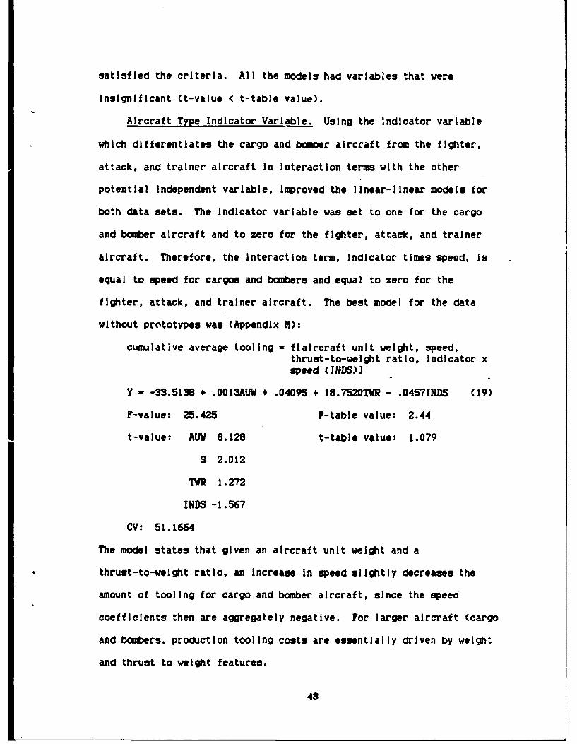
Aircraft Type Indicator Variable. Using the indicator variable

which differentiates the cargo and bomber aircraft from the fighter,

attack, and trainer aircraft In Interaction terms with the other

potential Independent variable, improved the linear-linear models for

both data sets. The Indicator variable was set to one for the cargo

and bomber aircraft and to zero for the fighter, attack, and trainer

aircraft. Therefore, the interaction term, indicator times speed, Is

equal to speed for cargos and bombers and equal to zero for the

fighter, attack, and trainer aircraft. The best model for the data

without prototypes was (Appendix M):

cumulative average tooling - f[alrcraft unit weight, speed,thrust-to-welght ratio, Indicator xspeed (INDS)]

Y - -33.5138 + .O013AUW + .04095 + 18.7520TWR - .04571NDS (19)

F-value: 25.425 F-table value: 2.44

t-value: AUW 8.128 t-table value: 1.079

S 2.012

TWR 1.272

INDS -1.567

CV: 51.1664

The model states that given an aircraft unit weight and a

thrust-to-weight ratio, an increase In speed slightly decreases the

amount of tooling for cargo and bomber aircraft, since the speed

coefficients then are aggregately negative. For larger aircraft (cargo

and bombers, production tooling costs are essentially driven by weight

and thrust to weight features.

43

The best model for the data with the prototype data was (Appendix

N):

cumulative average tooling - f(aircraft unit weight, speed,indicator x speed)

Y - -13.0647 + .0011AUW + .0543S - .0309INDS (20)

F-value: 46.199 F-table value: 2.53

t-value: AUW 8.863 t-table value: 1.076

S 3.103

IIIDS -1.234

CV: 34.6433

This model Implies that given an aircraft unit weight, an increase In

speed will increase the amount of required tooling much less for cargo

and bomber aircraft than for fighter, attack, and trainer aircraft.

Summary, Since the models with the interaction terms with the

Indicator for aircraft system types meet ill the criteria and have

lower CV values than the linear-linear models selected above, they

fit the data to the line best. Since the CYs are lower than the

representative differences (RDs) for the DAPCA III model, these models

are better able to estimate the amount of tooling for future aircraft

airframes.

DAPCA III (RD) Linear-linear (CV)

Without Prototypes 62.00% 51.17%

With Prototypes 54.62% 34.64%

Learnina Curve AdJustment. The linear-linear models selected will

provide the cumulative average cost of the first 100 airframes. The

amount of tooling required for other quantities can be obtained by

calculating the first unit cost using the following formula:

44

YA b (21)

100

where

A - first unit cost (hours)Y - cumulative average cost of first 100 airframes from Eqs (19)

or (20) (adJusted to hours)b - -0.5362 for the data without prototypes [Eq (19)] and

-0.6880 for the data Including prototypes (Eq (20)]b

100 - .0846 for the data without prototypes [Eq (19)] and.0421 for the data Including prototypes (Eq (20)]

Use this first unit cost (A) and Eq (12) to determine the cumulative

average hours for the number of airframes being estimated.

Alternative to Manufacturing Factor

When tooling was regressed against engineering (ENGR) and

manufacturing (MFG) for the data set without prototypes, engineering

was significant but manufacturing was not significant (Appendix 0):

cumulative total tooling = f(engineerlng, manufacturing)

Y = 110.4863 + 1.2842ENGR + .0162MFG (22)

F-value: 79.573 F-table valu(: 2.07

t-value: ENGR 7.057 t-table value: 1.074

MFG 0.421

CV: 26.2050

Manufacturing was significant when tooling was regressed against

engineering and manufacturing for the data set with prototypes

(Appendix P):

cumulative total tooling a f(engineering, manufacturing)

Y - 471.8331 + .6255ENGR + .1056 MFG (23)

F-value: 79.752 F-table value: 2.07

45

t-value: ENGR 5.981 t-table value: 1.074

MFG 2.804

CV: 25.1669

Historical Simulation. Since the number of observatfcnQ was

smal, when the most recent six observations were removed, six

observations from earlier models was added to the data set. The six

observations, which were removed, were: A-6, B-1, F-15, F-16, F-18,

and P-3. The six observations that were added are listed In Appendix

0, along with the CES lot data Information. There was a significant

change to the model for the data without the prototypes. Manufacturing

was significant In this model with older aircraft. In fact,_

manufacturing hours are more significant than engineering hours here.

cumulative total tooling - f(engineering, manufacturing)

Y = -427.307 + .7087ENGR + .1519MFG (24)

F-value: 65.710 F-table value: 2.07

t-value: ENGR 4.151 t-table value: 1.074

MFG 4.327

CV: 30.9549

When the simulation was run for the data with the prototypes there was

not a significant change, except that note again that manufacturing Is

more significant than engineering historically.

cumulative total tooling - f(englneering, manufacturing)

Y - 749.0991 + .4511SIHR + .1742HFG (25)

F-value: 87.537 F-table value: 2.07

t-value: ENGR 3.616 t-table value: 1.074

MFG 4.798

CV: 24.313

46

Summary. This analysis Indicates that for estimates of airframe

costs that do not include the effort for prototypes, there has been a

change in the relationship between tooling hours and engineering and

manufacturing hours. In the past, both engineering and manufacturing

were significant explanatory variables for tooling. However, more

recently only engineering is significant in predicting tooling needs.

The analysis also suggests that engineering and manufacturing are

both significant over time in explaining tooling needs when predicting

the requirements for airframe costs that include the effort for

prototypes.

Application Examples

To demonstrate and review the recommended cost estimating

equations, some tooling hour estimates are derived based on the

characteristics of a fictional aircraft. The fictional aircraft is a

cargo plane with airframe unit weight (AHPR weight In the DAPCA model)

of 110,000 pounds. Its speed (maximum mission speed at altltude In

knots) Is 500 miles per hour. Its thrust to weight ratio (military

static thrust of the engine at sea level In pounds, divided by airframe

unit weight) Is .42.

Example one. Estimate of the development tooling hours for 5

prototype aircraft airframes.

Method one. From Eq (16), ignoring the cargo characteristic,

the cumulative average tooling hours through unit 100 would be In

thousands of hours:

-4.829 + .00103(110,000) + .0445(500) = 130.721 or 130,720 hours

A more accurate estimate can be derived from Eq (20). It's

presumably a more accurate estimate since Its CV Is slightly lower.

47

The cumulative average tooling hours through unit 100 would be in

thousands of hours:

-13.0647 + .0011(110,000) + .0543(500) - .0309(500)= 119.64 or 119,640 hours

To derive the estimate for the cumulative average tooling hours of

the 5 prototypes use Eq (12) with X equal to 5 and A, b, and 100 raised

to the power of b are given by Eq (21):

A = 119.640 = 2,843,650 hours.0421

-.688cumulative average tooling hours = 2,843,650 x 5 = 939,690

So the tooling hour estimate for the 5 prototypes would be:

939,690 x 5 = 4,698,450 hours

Method two. Using estimates for the total engineering hours

and total manufacturing hours for the 5 prototypes, a total tooling

hour estimate for the 5 prototypes can be derived from Eq (23). Assume

the manufacturing estimate Is 10,800,000 hours and the engineering

estimate Is 5,400,000 hours. From Eq (23) the total cumulative tooling

estimate Is:

471,833 + .6255(5,400,000) + .1056(10,800,000) = 4,990,000 hours.

Whether the estimate of method one or two Is more reliable, depends on

the reliability of the manufacturing and engineering hour estimates.

Exmle to.. Assuming the same scenario as example one, to

estimate the tooling hours for the first 80 Prd2ion aircraft

airframes, use one of the following methods.

Metghdoe_. From Eq (15), ignoring the cargo characteristic,

cumulative average tooling hours through unit 100 would be in thousands

of hours:

48

-23.3537 + .0011(110,000) + .0263(500) + 21.3992(.42) = 117.784

or 117,784 hours

A more accurate estimate is derived from Eq (19). Cumulative

average tooling hours through unit 100 Is:

-33.5138 + .0013(110,000) + .0409(500) + 18.7520(.42) - .0457(500)- 114.962 or 114,962 hours

To determine the cumulative average tooling hours, use Eq (12)

with X equal to 80 and A, b, and 100 raised to the power of b given by

Eq (21):

A = 114,962 - 1,358,889.0846

-. 5362cumulative average tooling hours = 1,358,889 x 80 = 129,642

The tooling hour estimate for the first 80 airframes would be:

129,642 x 80 = 10,371,360 hours

Method two. Using estimates for the total engineering hours

ad the total manufacturing hours, an estimate of the total tooling

hours for the 80 production airframes can be derived using Eq (22).

Assume the total engineering hours estimate was 12,000,000 and the

total manufacturing hours estimate was 24,000,000 for the 80 airframes.

Using Eq (22) the total tooling hours would be:

471.8331 + .6255(12,000,000) + .1056(24,000,000)- 10,040,871 hours

Method thre.. If an accurate (error smaller than 10 percent)

total prototype cost estimate is also available, use the technique of

example one to derive total cost of development plus production of the

first 80 aircraft. Then subtract the prototype cost. In this

scenario, this method would be preferred, since the estimating error of

the equations with prototypes Is smaller than the estimating error of

the equations without prototypes.

49

V. Conclusions/Recommendations

Budget constraints have placed an increased emphasis on the

accuracy of DoD weapon system cost estimates. The DAPCA III model is

often used by Air Force personnel to estimate the tooling costs of

aircraft airframes. This study evaluates the accuracy, independent

variables, and data base of the DAPCA III model, and then provides

alternative models for estimating tooling for airframes.

Accuracy of DAPCA III, To determine the accuracy of the DAPCA III

model in estimating aircraft airframe tooling costs, the representative

difference was calculated for the data set both with and without

prototypes. The representative differences for the data with and

without prototypes, were 62.00 and 54.62 percent, respectively.

DAPCA III Independent Variables. The independent variables were

reviewed to determine If they are still logical variables for

estimating tooling costs of future aircraft airframes. Airframe unit

weight appears to be a good variable to explain the size of the

airframe. The variable speed captures the variations due to

performance. The performance characteristic thrust-to-weight ratio was

not used in DAPCA III but should capture variations due to

maneuverability of the aircraft systems.

DAPCA III does not have a variable for changes In production rate,

technology, or complexity. Careful consideration of each of these

factors indicated that they are difficult to quantify . Therefore,

it Is logical that they were not included In DAPCA III.

50

There are not any Indicator variables in DAPCA III. Other studies

have shown that Indicator variables for aircraft type or DoD service

component (Air Force versus Navy) have been significant.

The method used to account for the learning effect for various

quantities of airframes was considered appropriate.

Overall, the variables used In DAPCA III seem logical; however,

there was a possibility that other variables might also be significant.

These variables include: wing area, thrust-to-weight ratio, and

Indicator variables.

DAPCA III Data Base. The data base used in DAPCA III was updated

to Include more current aircraft systems.

Alternative Models. Although Rand found that the logarithm-linear

form fit the data best, the best models found In this study had a

linear-linear form. Models were developed using the data both with and

without the prototypes Included (Eqs (18) and (19)].

For both models, an indicator variable for aircraft type was

significant when used In an Interaction term with speed. This

indicates that changes In speed Impact tooling differently for cargo

and bombers than for fighter, attack, and trainer aircraft. An

analysis with Indicator variables for Air Force versus Navy did not

Improve the models.

This study Indicates that Eqs (18) and (19) are more accurate than

DAPCA III (51.17 and 34.64 percent, respectively).

Alternative to Manufacturino Factor. When tooling Is regressed

against engineering and manufacturing the relationship between the

variables becomes apparent. For the data without the prototypes only

engineering is significant. Both engineering and manufacturing are

51

significant for the data including the prototypes. In the past

manufacturing was more significant for both data sets. This suggests

that engineering drives the amount of tooling more than manufacturing.

Recommendations for Further Research

1. In light of the findings in this study, the other equations in

DAPCA III should be updated.

2. Several assumptions were needed to identify which lot data

In the CES contained prototype data. Since this study Indicates that

results differ depending on whether prototype data Is Included,

the data should be updated to clearly indicate prototypes.

3. The method used to adjust for the learning curve effort Is

adequate but cumbersome. It also leads to estimating error compounding

(the estimating error of the cost estimating model combined with the

estimating error of the learning curve). Alternate techniques to

handle the learning effect should be studied.

52

Appendix A: Comparison of DAPCA Data

DAPCA I DAPCA 11 DAPCA III

A-3J A-3 A-3B-52 A-4 A-4B-58 A-5 A-5B-66 A-7A A-67-3H A-7B A-7F-84 B-47 B-52F-84F B-52 B-58F-86 B-58 RB-66F-86D B-66 F-3F-89 F-3 F-4F-100 F-4 F-6F-101 F-84 F-14F-102 F-84F F-100F-104 F-86 F-102F-105 F-86D F-104F-106 F-89 F-105T-38 F-100 F-106

F-101 F-111F-102 T-38F-104 T-39P-105 C-5F-106 C-130F-111 C-133C-124 C-141C-130 KC-135C-133C-141

IC-135OV-10

53

Appendix B: Input Data for DAPCA III

MODEL AMPR WT SPEED OUANTITY

A-3 23104 544 50A-4 4987 545 165A-5 22900 1147 25A-6 17176 530 473A-7 11522 595 199B-52 133056 551 195B-58 32400 1147 116B-66 28551 548 59F-3 10400 460 265F-4 18100 1283 540F-6 8845 581 419F-14 26500 1170 577F-100 14087 775 1274F-102 12000 680 847F-104 8170 1150 230F-105 17954 1192 610F-106 14630 1153 277F-111 32926 1262 235T-38 5350 699 492T-39 7027 468 149C-5 279145 480 76C-130 43431 315 231C-133 97610 302 15C-141 104300 491 279

KC-135 70378 527 426

54

Appendix C: DAPCA III Representative Difference (without Prototypes)

2MODEL DIFFERENCE (DIFFERENCE)

A-3 693.1 480,387.6A-4 -1,861.3 3,464,437.7A-5 3,619.7 13,102,228.1A-6 2,705.3 7,318,648.1A-7 3,137.5 9,843,906.3B-52 13,257.6 175,763,957.8B-58 -7,390.6 54,620,968.4B-66 4,106.2 16,860,878.4F-3 1,874.1 3,512,250.8F-4 8,964.1 80,355,088.8F-6 -6,619.6 43,819,104.2F-14 -551.9 304,593.6F-100 806.4 650,281.0F-102 1,211.6 1,467,974.6F-104 2,955.1 8,732,616.0F-105 6,318.7 39,925,969.7F-106 1,455.6 2,118,771.4F-111 -5,414.0 29,311,396.0T-38 -153.4 23,531.6T-39 1,070.2 1,145,328.0C-5 2,774.3 7,696,740.5C-130 -1,144.2 1,309,193.6C-133 6,257.0 39,150,049.0C-141 11,603.2 134,634,250.2

KC-135 -1,884.9 3,552,848.0

55

Appendix D: DAPCA III Representative Difference (with Prototypes)

2MODEL DIFFERE4CE (DIFFERENCE)

A-3 231.1 53,407.2A-4 -2,021.0 4,084,441.0A-5 3,619.7 13,102,228.1A-6 923.8 853,406.4A-7 3,137.5 9,843,906.3B-52 13,257.6 175,763,957.8B-58 -7,390.6 54,620,968.4B-66 4,106.2 16,860,878.4F-3 1,658.7 2,751,285.7F-4 8,964.1 80,355,088.8F-6 -6,880.1 47,335,776.0F-14 -6,428.9 41,330,755.2F-100 806.4 650,281.0F-102 -6,403.8 41,008,654.4F-104 2,955.1 8,732,616.0F-105 6,318.7 39,925,969.7F-106 1,455.6 2,118,771.4F-111 -5,414.0 29,311,396.0T-38 -799.2 638,401.0T-39 1,070.2 1,145,328.0C-5 -396.4 f57,133.0C-130 -3,190.8 10,181,204.6C-133 6,189.8 38,313,624.0C-141 6,691.8 44,780,187.2

IC-135 -2,437.9 5,943,356.4

56

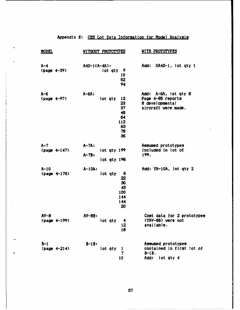
Appendix E: CES Lot Data Information for Model Analysis

MODEL WITHOUT PROTOTYPES WITH PROTOTYPES

A-4 A4D-I(A-4A): Add: XA4D-I, lot qty I(page 4-39) lot qty 9

105294

A-6 A-6A: Add: A-6A, lot qty 8(page 4-97) lot qty 12 Page 4-85 reports

23 8 developmental37 aircraft were made.4864

112637836

A-7 A-7A: Assumed prototypes(page 4-147) lot qty 199 Included In lot of

A-7B- 199.lot qty 196

A-10 A-IOA: Add: YA-IOA, lot qty 2(page 4-176) lot qty 6

223043

1014414420

AV-8 AV-8B: Cost data for 2 prototypes(page 4-199) lot qty 4 (YAV-8B) were not

12 available.18

B-1 B-IB: Assumed prototypes(page 4-214) lot qty I contained In first lot of

7 B-lB.10 Add: lot qty 4

57

WITHOUT PROTOTYPES WITH PROTOTYP

C-5 C-5A: Assumed prototypes(page 4-297) lot qty 8 contained In first lot of

18 C-SA.27 Add: lot qty 523

C-141 C-141A: Assumed prototypes(page 4-345) lot qty 145 contained In first lot of

134 C-141A.Addt lot qty 5

E-2 1-2C: Assumed first lot of E-2C(page 4-362) lot qty 11 contained prototypes.

8 Add: lot qty 29661166610

F-5 -5E: Assumed first lot of F-59(page 4-482) lot qty 21 contained prototypes.

16 Add: lot qty 5214

5?40554812

F-14 F-14A: Assumed first 2 lots of(page 4-513) lot qty 26 F-14A were prototypes.

48 Add: lot qty 648 650

3050503645443630303024

58

WITHOUT PROTOTYPES WITH PROTOTYPES

F-15 F-15A/B: Assumed prototypes(page 4-544) lot qty 20 Included in lot of 20.

306272

13221

108

F-16 F-16A/B: Assumed first lot of F-16A/B(page 4-575) lot qty 55 contained prototypes.

105 Add: lot qty 814575

348175180160

F-18 F/A-18A: Assumed first lot of F-18A(page 4-599) lot qty 9 contained prototypes.

25 Add: lot qty 11606318

178484

F-111 F-i11A: Assumed prototypes(page 4-798) lot qty 18 Included In lot of 18.

14176

59

WITHOUT PROTOTYPES WITH PROTOTYPES

P-3 P-3C: Assumed prototypes(page 4-845) lot qty 24 Included in lot of 24.

232412241212121115101412123124124635

S-3 S-3A: Assumed first lot of S-3A(page 4-881) lot qty 13 contains prototypes.

35 Add: lot qty 8454541

T-38 T-38A: Add: YT-38, lot qty 2(page 4-898) lot qty 4

1350144144137

60

Appendix F: Alternative Model Independent Variables

AIRFRAME THRUST-TO-MODEL UNIT WEIGHT WING AREA SPEED WEIGHT RATIO

A-4 4,987 260.0 545 1.4036

A-6 17,176 528.8 530 0.4949

A-7 11,522 375.0 595 0.9851

A-1O 14,842 506.0 423 0.5383

AV-8 7,662 230.0 486 2.1480

B-1 146,717 1950.0 1518 0.0891

C-5 279,145 6200.0 480 0.1462

C-141 104,300 3228.1 491 0.1822

E-2 22,800 700.0 302 0.1916

F-5 7,180 186.0 940 0.4875

F-14 26,500 565.1 1170 0.4660

F-15 17,642 608.0 1434 0.8148

F-16 10,104 300.0 1265 1.4519

F-18 16,070 400.0 990 0.6601

F-111 32,926 525.0 1262 0.3265

P-3 44,532 1300.0 382 0.1051

S-3 19,248 598.0 393 0.3600

T-38 5,350 170.0 699 0.5009

61

Appendix G: CES Lot Data Information for Learnina Curves

MODEL WITHOUT PROTOTYPES WITH PROTOTYPES

A-4 A4D-1: Add: XA4D-1, lot qty 1(page 4-39) lot qty 9

105294

A-6 A-6A: Add: A-6A, lot qty 8(page 4-97) lot qty 12

233?48

A-7 A-7A: No change.(page 4-147) lot qty 199

A-7B:lot qty 196

A-1O A-IOA: Add: YA-IOA, lot qty 2(page 4-176) lot qty 6

223043

AV-8 AV-8B: No change.(page 4-199) lot qty 4

1218

B-i B-IB: Add: B-1B, lot qty 4(page 4-214) lot qty 1

710

C-5 C-BA: Add: C-5A, lot qty 5(page 4-297) lot qty 8

18

2723

C-141 C-141A: Add: C-141A, lot qty 5(page 4-345) lot qty 145

134

62

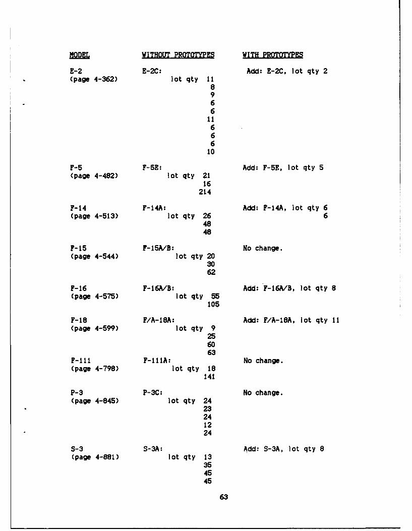
WITHOUT PROTOTYPES WITH PROTOTYPES

E-2 E-2C: Add: E-2C, lot qty 2(page 4-362) lot qty 11

89661166610

F-5 F-5E: Add: F-5E, lot qty 5(page 4-482) lot qty 21

16214

F-14 F-14A: Add: F-14A, lot qty 6(page 4-513) lot qty 26 6

4848

F-15 F-i5A/B: No change.(page 4-544) lot qty 20

3062

F-16 F-16A/B: Add: F-16A/B, lot qty 8(page 4-575) lot qty 55

105

F-18 F/A-18A: Add: F/A-18A, lot qty 11(page 4-599) lot qty 9

256063

F-111 F-lilA: No change.(page 4-798) lot qty 18

141

P-3 P-3C: No change.(page 4-845) lot qty 24

23241224

S-3 S-3A: Add: S-3A, lot qty 8(page 4-881) lot qty 13

354545

63

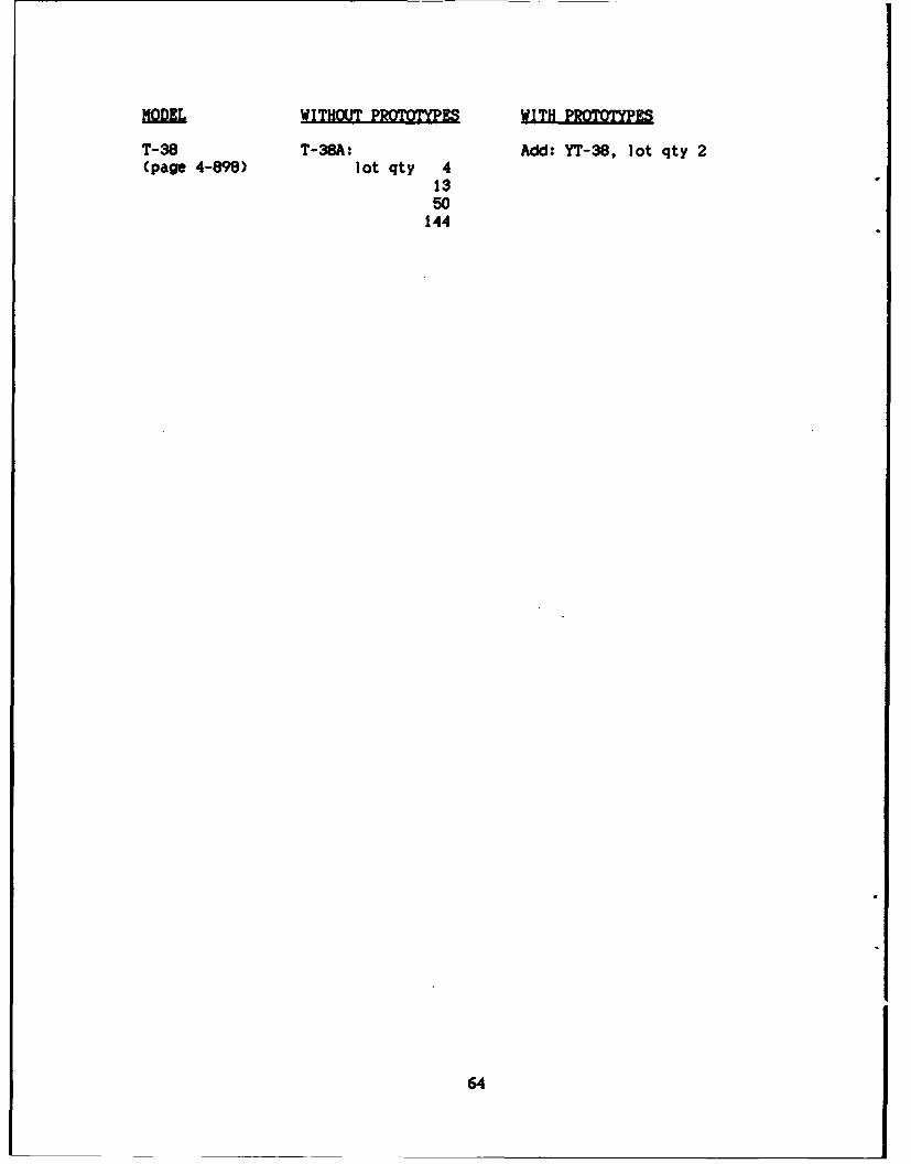
mmWITHOUT PROTY~PES WITH PROTOTYPES

T-38 T-38A: Add: YT-38, lot qty 2(page 4-898) lot qty 4

1350144

64

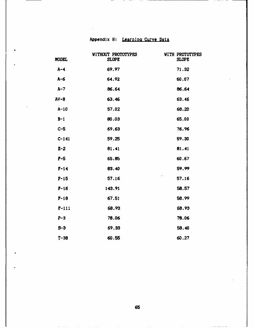
Appendix H: Learning Curve Data

WITHOUT PROTOTYPES WITH PROTOTYPESMODEL SLOPE SLOPE

A-4 69.97 71.32

A-6 64.92 60.07

A-7 86.64 86.64

AV-8 63.46 63.46

A-1O 57.02 68.20

B-1 80.03 65.00

C-5 69.63 76.96

C-141 59.25 59.30

E-2 81.41 81.41

F-5 65.85 60.67

F-14 83.40 59.99

F-15 57.16 57.16

F-16 143.91 58.57

F-18 67.51 58.99

F-111 68.93 68.93

P-3 78.06 78.06

S-3 69.33 58.40

T-38 60.55 60.27

65

Appendix I: Linear-Linear Model SAS Output (without Prototypes)

Tooling = f(AUW, S, TVR)

ANALYSIS OF VARIANCES

SUN Or MEANSOURCE DF SQUARES SQUARE F VALUE PROB>F

MODEL 3 88837.08095 29612.36032 29.967 0.0001ERROR 14 13834.36495 988.16893C TOTAL 17 102671.44590

ROOT MSE 31.43515 R-SQUARE 0.8653DEP MEAN 58.47369 ADJ R-SO 0.8364C.V. 53.75949

PARAMETER ESTIMATES

PARAMETER STANDARD T FOR HO:VARIABLE DF ESTIMATE ERROR PARAMETER=0 PROB > ITI

INTRCEP 1 -23.3537 20.83122 -1.121 0.2811AUW 1 0.0011 0.00012 8.942 0.0001S 1 0.0263 0.01898 1.388 0.1869TWR 1 21.3992 15.38684 1.391 0.1860

VARIABLE N MEAN STD DEV SUN MINIMUM MAXIMUM

TOOL 18 58.47 77.71 1052.5 F.582 321.3AUW 18 43816.83 69413.94 788703.0 4987.000 279145.0S 18 772.50 401.71 13905.0 302.000 518.0TWR 18 0.63 0.55 11.4 0.089 2.1

66

Appendix J: Linear-Llnear Model SAS Output (with Prototves)

Tooling - f(AUW, S)

ANALYSIS OF VARIANCE

SUM OF MEANSOURCE DF SQUARES SQUARE F VALUE PROB>

MODEL 2 91523.29255 45761.64628 66.235 0.0001ERROR 15 10363.53837 690.90256C TOTAL 17 101886.83092

ROOT MSE 26.28503 R-SOUARE 0.8983DEP MEAN 74.58769 ADJ R-SO 0.8847C.V. 35.24043

PARAMETER ESTIMATES

PARAMETER STANDARD T FOR HO:VARIABLI DF ESTIMATE ERROR PARAMETER=0 PROB > ITI

INTERCE P 1 -4.82863 14.34419 -0.337 0.7411AUW 1 0.00103 0.00009 11.187 0.00015 1 0.04453 0.01587 2.806 0.0133

VARIABLE N MEAN STD DEV SUM MINIMUM MAXIMUM

TOOL 18 74.59 77.42 1342.6 5.582 320.2AUW 18 43816.83 69413.94 788703.0 4987.000 279145.0S 18 772.50 401.71 13905.0 302.000 1518.0

67

Appendix K: Outlier Diagnostic Data (without PrototyDes)

STUDENTI ZEDDELETED

MODEL LEVERAGE RESI DUAL COOK' S D

A-4 0.1917 -0.3353 0.0071

A-6 0.0979 -0.0429 0.0001

A-7 0.0943 -0.6695 0.0122

A-1O 0.1191 0.3007 0.0032

AV-8 0.5690 1.4577 0.6491

B-1 0.3995 -1.0178 0.1718

C-5 0.7897 1.7209 2.4382

C-141 0.1411 -1.5953 0.0941

E-2 0.2026 1.0066 0.0642

P-5 0.1002 -0.3132 0.0029

F-14 0.1297 -0.2317 0.0022

F-15 0.2242 0.8195 0.0497

F-16 0.2719 -1.5710 0.2036

F-18 0.0833 -1.3493 0.0030

F-111 0.1740 3.4378 0.3512

P-3 0.1746 -0.8483 0.0388

S-3 0.1449 0.2637 0.0032

T-38 0.0923 -0.0553 0.0001

68

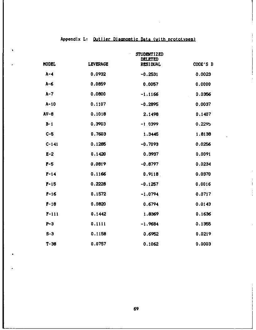
Appendix L: Outlier Dlaanostic Data (with prototypes)

STUDENTIZEDDELETED

MODEL LEVERAGE RESIDUAL COOK"S D

A-4 0.0932 -0.2531 0.0023

A-6 0.0859 0.0057 0.0000

A-7 0.0800 -1.1166 0.0356

A-10 0.1107 -0.2895 0.0037

AV-8 0.1018 2.1498 0.1407

B-1 0.3903 -1 0399 0.229b

C-5 0.7603 1.3445 1.8138

C-141 0.1285 -0.7093 0.0256

E-2 0.1420 0.3937 0.0091

F-5 0.0819 -0.8797 0.0234

F-14 0.1166 0.9118 0.0370

F-15 0.2228 -0.1257 0.0016

F-16 0.1572 -1.0794 0.0717

F-18 0.0820 0.6794 0.0143

F-111 0.1442 1.8369 0.1636

P-3 0.1111 -1.9684 0.1355

S-3 0.1158 0.6952 0.0219

T-38 0.0757 0.1062 0.0003

69

Appendix M: Alternative Model SAS Output (without Protatypes)

Tooling - f(AUW, S, TWR, INDS)

ANALYSIS OF VARIANCE

SUN OF MEANSOURCE DF SQUARES SUARE F VALUE PROB>F

MODEL 4 91034.63501 22758.65875 25.425 0.0001ERROR 13 11W36.81089 895.13930C TOTAL 17 102671.44590

ROOT MSE 29.91888 R-SOUARE 0.8867DEP MEAN 58.47369 ADJ R-SO 0.8518C.V. 51.1664

PARAMETER ESTIMATES

VARIABLE DF ESTIMATE ERROR PARAMETER=O PROB > ITI

INTERCEP 1 -33.5138 20.85989 -1.607 0.1321AUW 1 0.0013 0.00015 8.128 0.0001S 1 0.0409 0.02031 2.012 0.0654TWR 1 18.7520 14.74179 1.272 0.2256INDS 1 -0.0457 0.02916 -1.567 0.1412

70

Appendix N: Alternative Model SAS Output (with Prototypes)

Tooling = f(AUW, S, INDS)

ANALYSIS OF VARIANCE

SUM OF MEANSOURCE DF SQUARES SQUARE F VALUE PROB>F

MODEL 3 92539.21210 30846.40403 46.199 0.0001ERROR 14 9347.61883 667.68706C TOTAL 17 101886.83092

ROOT MSE 25.83964 R-SQUARE 0.9083DEP MEAN 74.58769 ADJ R-SO 0.8886C.V. 34.64330

PARAMETER ESTIMATES

VARIABLE DF ESTIMATE ERROR PARAMETER=0 PROB > ITI

INTERCEP 1 -13.0647 15.60196 -0.837 0.4164AUW 1 0.0011 0.00013 8.863 0.0001S 1 0.0543 0.01750 3.103 0.0078INDS 1 -0.0309 0.02502 -1.234 0.2377

71

Appendix 0: TOOL/ENGR/MFG Model SAS Output (without Prototves)

Tooling = f(ENGR, MFG)

ANALYSIS OF VARIANCE

SUN OF MEANSOURCE DF SQUARES SQUARE F VALUE PROB>F

MODEL 2 689411923.72 344705961.86 79.573 0.0001ERROR 15 64979000.78 4331933.39C TOTAL 17 754390924.50

ROOT MSE 2081.33 R-SQUARE 0.9139DEP MEAN 7942.50 ADJ R-SO 0.9024C.V. 26.20497

PARAMETER ESTIMATES

PARAMETER STANDARD T FOR HO:VARIABLE DF ESTIMATE ERROR PARAMETER.0 PROB > ITI

INTERCEP 1 110.4863 875.6260 0.126 0.9013ENGR 1 1.2842 0.1820 7.057 0.0001MFG 1 0.0162 0.0384 0.421 0.6795

VARIABLE N MEAN STD DEV SUm MINIMUM MAXIMUM

TOOL 18 7942.50 6661.53 142965.0 2090.00 25399.00ENGR 18 5693.89 4727.68 102490.0 782.00 19226.00MFG 18 32190.00 22432.06 579420.0 4407.00 74562.00

72

Appendix P: TOOL/ENGI/MFG Model SAS Output (with Prototypes)

Tooling - f(ENGR, MFG)

ANALYSIS OF VARIANCE

SUM OF MEANSOURCE DF SQUARES SQUARE F VALUE PROB>F

MODEL 2 1026713347 513356673.41 79.752 0.0001ERROR 15 96553227 6436911.13C TOTAL 17 1123267014

ROOT MSE 2537.107 R-SOUARE 0.9140DEP MEAN 10081.110 ADJ R-SQ 0.9026C.V. 25.16694

PARAMETER ESTIMATES

PARAMETER STANDARD T FOR HO:VARIABLE DF ESTIMATE ERROR PARAHETER-O PROB > ITI

INTERCEP 1 471.8331 1057.9623 0.446 0.6620ENGR 1 0.6255 0.1046 5.981 0.0001MFG 1 0.1056 0.0377 2.804 0.0134

VARIABLE N MEAN STD DEV SUM MINIMUM MAXIMUM

TOOL 18 10081.11 8128.62 181460.0 2090.0 28911.0ENGR 18 9412.06 8952.00 169417.0 782.0 33599.0MFG 18 35257.39 24863.01 634633.0 4407.0 88767.0

73

Appendix 0: CES Lot Data Information forHistorical Simulation

WITHOUT PROTOTYPES WITH PROTOTYPES

A-5 A-5A: Assumed prototypes(page 4-73) lot qty 11 Included In lot of 11.

14

B-58 B-58A: Add: B-58A, lot qty 13(page 4-265) lot qty 17

362030

F-4 F-4A: Add: F-4A, lot qty 7(page 4-411) lot qty 16

24

F-104 F-104A: Add: XF-104A, lot qty 2(page 4-734) lot qty 17

F-i 04B:lot qty 6

F-I 04A/C:lot qty 209

F-I 04C:lot qty 21

F-105 F-1053: Add: YF-105A/B, lot qty 15(page 4-752) lot qty 65

11C-135 KC-135A: Add: KC-135, lot qty 1(page 4-824) lot qty 29

6811813081

74

1. Actual Detail Weight and Balance Report For Model B-1B AirVehicle. Report NA 87-1600. Rockwell International,March 4, 1988.

2. Batchelder, C. A. and others. An Introduction To EquiDment CostEstimates. Report No. RM-6103-SA. Santa Monica CA: The RandCorporation, December 1969.

3. Beck, Charles L. and Dennis L. Pfeil. Airframe RDT&E CostEstimating: A Justification For And Development of Unique CostEstimating Relationships According to Aircraft Type. School ofSystems and Logistics, Air Force Institute of Technology (AU),Wright-Patterson AFB OH, September 1982.

4. Bennett, Bruce Robert. The Use of Parametric Cost EstimatingRelationships as They Pertain to Aircraft Airframes; A NewPerspective. Naval Postgraduate School, March 1980.

5. Birkler, J. L. and others. Development And Production CostEstlmatlna Relationships For Aircraft Turbine Enalnes. Report No.N-1882-AF. Santa Monica CA: The Rand Corporation, October 1982.AD-A123753.

6. Blucker, Rick and others. Advanced Tactical Fighter ProgramEstimate. Wright Patterson Air Force Base OH: AeronauticalSystems Division, November 1984.

7. Boren, H. E., Jr. A Computer Model for Estimating Developmentand Procurement Costs of Aircraft. Report No. R-1854-PR. SantaMonica CA: The Rand Corporation, March 1976. AD-A025276.

8. Carrier, J. M. and R. W. Smith. Aircraft Airframe Cost EstimatinaTechniques. Report No. RM-3375-PR. Santa Monica CA: The RandCorporation, November 1962. AD-293863.

9. Cook, Thomas M. and Robert A. Russell. Contemporary OperationsManacement (2nd edition). Englewood Cliffs NJ: Prentice-Hall,Inc., 1984.

10. Cost Estimatina System. Volume 2 Aircraft Cost Handbook. Book 1:Aircraft. Arlington VA: DELTA Research Corporation, November1987.

11. Daneman, Jeffrey. mHow Good Is Our LSBF Equation at Predicting.'Journal of Parametrics, Vol V1, No 3 (September 1986).

12. Day, C. F. and D. P. 2indley. Aircraft Cost Handbook. ReportNo. FR-1834-USAF. Arlington VA: J. Watson Noah, Inc., December1982.

75

13. Donlan, Thomas G. 'Collision Course, Expensive New WeaponsPrograms vs the Budget.' Barron's: 16, 34-35 (August 17, 1987).

14. Dreyfuss, David J. and Joseph P. Large. Estimated Costs ofExtended Low-Rate Airframe Production. Report No. R-2243-AF.Santa Monica CA: The Rand Corporation, March 1978.

15. Garfinkle, Jeffrey B. and John L. Blrkler. Regression DiaanosticsIn Practice--Experlences From Modellina Jet Enaine Costs. ReportNo. P-6896. Santa Monica CAt The Rand Corporation, June 1983.AD-A154199.

16. Hildebrandt, Gregory G. and Man-bing Sze. Accounting For TheCost of Tactical Aircraft. Report No. N-2420-PA&E. Santa MonicaCA: The Rand Corporation, December 1974.

17. Hinch, James H., Capt, USAF. Aircraft Airframe Cost EstimationUsina a Random Coefficients Model. School of Systems andLogistics, Air Force Institute of Technology (AU), Wright-Patterson AFB OH, December 1979.

18. Hutchison, Larry D. A Microcomputer Program For the Solution ofLearnina Curve Computations. School of Systems and Logistics, AirForce Institute of Technology (AU), Wright-Patterson AFB OH,September 1985.

19. Kage, Gordon D. II, MaJor, USAF. Estimatina The Cost ofCoamosite Material Airframes Using The Rand CorporationDevelopment And Procurement Cost of Aircraft Parametric Model(DAPCA III). School of Systems and Logistics, Air Force Instituteof Technology (AU), Wright-Patterson AFB OH, September 1983.

20. Kankey, Roland D. *Learning Curves: An Overview.' NationalEstimator, Vol 4, No. 2. Spring 1983.

21. Large, Joseph P. A Com©arlson of Cost Models for FighterAircraft. Report No. P-6011. Santa Monica CA: The RandCorporation, September 1977.

22. -------. Development of Parametric Cost Models for Weapon Systems.Report No. P-6604. Santa Monica CA: The Rand Corporation, April1981. AD-A105179.

23. Large, J. P. and Capt K. M. S. Gillespie. A Critique of AircraftAirframe Cost Models. Report No. R-2194-AF. Santa Monica CA:The Rand Corporation, September 1977. AD-A047181.

24. Large, Joseph P. and others. Parametric Eauations for EstimatinoAircraft Airframe Costs. Report No. R-1693-1-PA&E. SantaMonica CA: The Rand Corporation, February 1976. AD-A022086.

25. -------. Production Rate and Production Cost. Report No.R-1609-PA&E. Santa Monica CA: The Rand Corporation, December1974.

76

26. Levenson, G. S. and S. M. Barro. Cost-Estlmatlng Relationshipsfor Aircraft Airframes. Report No. RM-4845-PR. Santa Monica CA:The Rand Corporation, February 1966.

27. Levenson, G. S. and others. Cost-Estlmatina Relationships forAircraft Airframes. Report No. R-761-PR (Abridged). SantaMonica CA: The Rand Corporation, February 1972. AD-A012091.

28. Neter, John and others. Applied Linear Statistical Models (2ndedition). Homewood, IL: Richard D. Irwin, Inc., 1985.

29. Noah, J. W., and others. Estimatina Aircraft Acqulsition CostsBy Parametric Methoas. J. Watson Noah Associates, Inc.,FR-103-USN, September 1973.

30. Predicted Performance of B-1B Production Aircraft. ReportNA-84-1143. Rockwell International, February 22, 1984.

31. Potler, K. H. Actual Weiaht Report. Intermediate Aircraft. ForModel C-130A (TAC) Medium Rance Carao and Troop Carrier AircraftReport No. ER 2342. Lockheed Aircraft Corporation,January 25, 1957.

32. Robbins, Jane L. Learnina Curve Theory and Analysis. Visual AidsHandout. ONT 180. School of Systems and Logistics, Air ForceInstitute of Technology (AU), Wright-Patterson AFB OH, August1983.

33. Sanchez, Luls R. and Jarnes A. Del Rossl. Methods of EstimatingFlxed-Wlno Airframe Costs: Volume I (Revised). Report No.PRC R-547A. Los Angelos CA: Planning Research Corporation, April1967.

34. SAS Institute Inc. SAS User's Guide: Statistics. Version 5EditLon. Cary NC: SAS Institute Inc. 1985.

35. Stlglltz, Joseph E. Economics of the Public Sector (Ist edition).W. W. Norton and Co., 1986.

36. Timson, F. S. and D. P. Tlhansky. Confidence In EstimatedAirframe Costs: Uncertainty Assessment In Aaareaate Predictions.Repn. No. R-903-PR. Santa Monica CA: The Rand Corporation,October 1972. AD-757503.

37. Westrlch, James. Cost Analyst. Telephone Interview. Researchand Cost, Directorate of Cost, Aeronautical Systems Division.December 7, 1987.

38. Womer, Norman Keith. 'An Automated Airframe Production CostModel.' Proceedinas fo the 1983 Federal Acaulsition ResearchSyosium, December 1983. AD-A137700.

77

39. -------. 'A Cost Function For Military Airframes.' Invitedaddress. Ninth Annual DoD/FAI Acquisition Research Symposium,9-11 June 1980, Anapolls MD. AD-A097538.

40. Womer, N. Keith and Thomas R. Gulledge. Cost Functions forAirframe Production Proarams. Air Force Business ManagementOffice Contract F33615-81-K-5116. July 1982. AD-A119788.

78

VITA

Captain Patricla L. Meyer received a Bachelor of Arts in

Management from St. Martin's College, Lacey, Washington In May 1982.

At that time, she received her commission in the Air Force through the

ROTC program. Fran September 1982 until June 1985 she was assigned to

Hanscom AFB, Massachusetts. While at Hanscom she worked as a program

analyst on the Space Defense Operations Center Program and as a cost

estimating project officer for the Strategic Command and Control

Systems Directorate. From July 1985 until May 1987 she was the Chief

of the Cost Branch at Grissom AFB, Indiana. In June 1987 she entered

the School of Systems and Logistics, Air Force Institute of Technology.

79

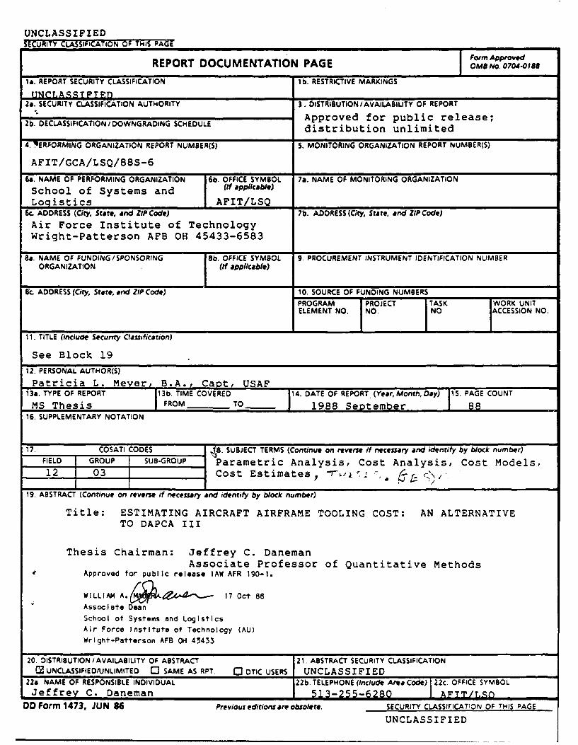
UNCLASSIFIEDSECURITY CLASSIFICATION OF THIS PAGE

Form ApprovedREPORT DOCUMENTATION PAGE OMB No. 07040188

la. REPORT SECURITY CLASSIFICATION lb. RESTRICTIVE MARKINGS

PNCA S PT r__2a. SECURITY CLASSIFICATION AUTHORITY 3. DISTRIBUTION /AVAILABILITY OF REPORT2b. DECLASSIFICATION/DOWNGRADING SCHEDULE Approved for public release;

distribution unlimited4. 1ERFORMING ORGANIZATION REPORT NUMBER(S) S. MONITORING ORGANIZATION REPORT NUMBER(S)

AFIT/GCA/LSQ/88S-6

6a. NAME OF PERFORMING ORGANIZATION 6b. OFFICE SYMBOL 7a. NAME OF MONITORING ORGANIZATION

School of Systems and (If ppllcable)

Logistics I AFIT/LSQ6c. ADDRESS (City, State, and ZIP Code) 7b. ADDRESS (City, State, and ZIP Code)

Air Force Institute of TechnologyWright-Patterson AFB OH 45433-6583

Ba. NAME OF FUNDING/SPONSORING 8b. OFFICE SYMBOL 9. PROCUREMENT INSTRUMENT IDENTIFICATION NUMBERORGANIZATION (If applicable)

8c. ADDRESS (City, State, and ZIP Code) 10. SOURCE OF FUNDING NUMBERSPROGRAM PROJECT TASK WORK UNITELEMENT NO. NO. NO ACCESSION NO.

11. TITLE (Include Security Classification)

See Block 19

12. PERSONAL AUTHOR(S)

Patricia L. Meyer B.A., Capt, USAF13a. TYPE OF REPORT 13b. TIME COVERED 14. DATE OF REPORT. (Year, Month,Day) IS. PAGE COUNT

MS Thesis FROM TO 1988 September 816. SUPPLEMENTARY NOTATION

17. COSATI CODES ,1. SUBJECT TERMS (Continue on reverse if necessary and identify by block number)FIELD GROUP SUB-GROUP Parametric Analysis, Cost Analysis, Cost Models,12 03 Cost Estimates - _ , - .

19. ABSTRACT (Continue on reverse if necessary and identify by block number)

Title: ESTIMATING AIRCRAFT AIRFRAME TOOLING COST: AN ALTERNATIVETO DAPCA III

Thesis Chairman: Jeffrey C. DanemanAssociate Professor of Quantitative Methods

Approved for public release IAW AFR 190-1.

WILLIAM A. ( ?XA - 17 Oct 88Associate Dean

School of Systems and Logistics

Air Force Institute of Technology (AU)

Wright-Patterson AFB OH 45433

20. DISTRIBUTION/AVAILABILITY OF ABSTRACT 21. ABSTRACT SECURITY CLASSIFICATIONC" UNCLASSIFIED/UNLIMITED 0 SAME AS RPT. C: DTIC USERS UNCLASSIFIED

22a. NAME OF RESPONSIBLE INDIVIDUAL 22b. TELEPHONE (Include Area Code) 22c, OFFICE SYMBOLJeffrey C. Daneman 513-255-6280 AFTT/T.

DO Form 1473, JUN 86 Previous editions are obsolete. SECURITY CLASSIFICATION OF THIS PAGE

UNCLASSIFIED

UNCLASSIFIED

The purpose of this study was to evaluate the tooling costestimating equation of the DAPCA III model and determine If moreaccurate models can be developed. The five objectives of the researchwere: (I) Determine the accuracy of the DAPCA III model. (2)Determine If the Independent variables In DAPCA III are logicallyvalid. (3) Determine If the data base which was used to develop DAPCAIII is appropriate for estimating today's aircraft systems. (4)Determine If the accuracy of the DAPCA III model can be Improved. (5)Determine If using a factor of manufacturing is sufficient to estimatetooling costs.-,

The study found that the accuracy of the DAPCA III model can beImproved by Including additional variables and updating the data base.More accurate models were developed for the data base both Includingand excluding the prototype aircraft systems.

When tooling was regressed against manufacturing and engineering,the data without the prototypes Indicated that engineering was moresignificant than manufacturing. Both manufacturing and engineeringwere significant for the data with the prototypes. , 1

UNCLASSIFIED