learning to run a power network challenge for training

HAL Id: hal-03159692https://hal.inria.fr/hal-03159692

Submitted on 4 Mar 2021

HAL is a multi-disciplinary open accessarchive for the deposit and dissemination of sci-entific research documents, whether they are pub-lished or not. The documents may come fromteaching and research institutions in France orabroad, or from public or private research centers.

L’archive ouverte pluridisciplinaire HAL, estdestinée au dépôt et à la diffusion de documentsscientifiques de niveau recherche, publiés ou non,émanant des établissements d’enseignement et derecherche français ou étrangers, des laboratoirespublics ou privés.

Learning to run a power network challenge for trainingtopology controllers

Antoine Marot, Benjamin Donnot, Camilo Romero, Luca Veyrin-Forrer,Marvin Lerousseau, Balthazar Donon, Isabelle Guyon

To cite this version:Antoine Marot, Benjamin Donnot, Camilo Romero, Luca Veyrin-Forrer, Marvin Lerousseau, et al..Learning to run a power network challenge for training topology controllers. Electric Power SystemsResearch, Elsevier, 2020, 189, pp.106635. �10.1016/j.epsr.2020.106635�. �hal-03159692�

https://hal.inria.fr/hal-03159692

https://hal.archives-ouvertes.fr

Learning to run a power network challengefor training topology controllers

Antoine Marot, Benjamin DonnotCamilo Romero, Balthazar Donon

Reseau de Transport d’ElectriciteParis, France

Marvin LerousseauINSERM and CVN

CentraleSuplec and INRIAParis, France

Luca Veyrin-Forrer, Isabelle GuyonTAU group of Lab. de Res. en Informatique

UPSud/INRIA Universie Paris-SaclayParis, France

Abstract—For power grid operations, a large body of researchfocuses on using generation redispatching, load shedding ordemand side management flexibilities. However, a less costly andpotentially more flexible option would be grid topology recon-figuration, as already partially exploited by Coreso (EuropeanRSC) and RTE (French TSO) operations. Beyond previous workon branch switching, bus reconfigurations are a broader classof action and could provide some substantial benefits to routeelectricity and optimize the grid capacity to keep it within safetymargins. Because of its non-linear and combinatorial nature, noexisting optimal power flow solver can yet tackle this problem.We here propose a new framework to learn topology controllersthrough imitation and reinforcement learning. We present thedesign and the results of the first “Learning to Run a PowerNetwork” challenge released with this framework. We finallydevelop a method providing performance upper-bounds (oracle),which highlights remaining unsolved challenges and suggestsfuture directions of improvement.

Index Terms—Artificial Intelligence, Control, Power Flow,Reinforcement Learning, Competition

I. INTRODUCTION

Grid operators are in charge of ensuring that a reliablesupply of electricity is provided everywhere, at all times.However, their task is becoming increasingly difficult underthe current steep energy transition. On one hand, we observethe advent of intermittent renewable energies on the produc-tion side and of prosumers on the demand side, coupled tothe globalization of energy markets over a more and moreinterconnected European grid. This brings a whole new set ofactors to the power system, adding lots of uncertainties to it.On the other hand, recent improvements in terms of energyefficiency have put an end to the total consumption growth,and de facto to the growth in revenues, thus limiting new costlyinvestments. Public acceptance with regards to the installationof new infrastructure is also a growing issue. This shiftsthe way we traditionally develop the grid, from expandingits capacity by building new power lines, to optimizing theexisting one as it is, closer to its limits, with rather digitalmeans and every flexibilities at our disposal.

Currently, operators must analyze massive amounts of datato take complex coordinated decisions over time with higherreactivity, to operate under an ever more constrained envi-ronment with greater control. An under-exploited flexibility,which could alleviate in part the problem, is the grid topology,

as already pointed out by early work [1]. This avenue isexplored in the present paper. As of today, it is still beyondthe state-of-the-art to control optimally such grid topology “atscale”, beyond the level of “branch switching” [5] (e.g. consid-ering more complex actions such as “bus splitting”), becauseof the non-linear and combinatorial nature of the problem.Lately, we demonstrated an augmented expert system ability[9] to discover steady-state tactical solutions to unsecure gridstates by relying on bus splitting. Its acceptable computationaltime opens new perspectives for a revival of such class of ac-tions. In addition, novel and more flexible actions should alsobe considered today, intervening not only instantaneously as atactic rather independently of other decisions, but over a timehorizon as a strategy to manage more numerous overlappingand interfering decisions. To exploit such a complex arrayof actions, optimal control methods [5] have been exploredbut are hard to deploy in control rooms because of limitedcomputing budget constraints.

With the latest breakthroughs in Artificial Intelligence (AI)from AlphaGo at Go [15] and Libratus at Poker [2], DeepReinforcement Learning (RL) seems a promising avenue todevelop a control algorithm, a.k.a. an artificial agent, ableto operate a complex power system at scale near real-timeand over time, assisted by existing advanced physical gridsimulators. Recent work [3] has already shown the value ofDeep Learning for accelerating power flow computation andrisk assessment applications for power systems, demonstratingits ability to model such system behavior, adding more creditto the Deep RL potential. RL formulations have already beenapplied to specific power system related problems (see [7]for a review), but not for continuous power system real-time operations, a problem for which no test cases existedtoday, probably limiting any subsequent development. Relatedapplications concern the unit commitment problem with aninteresting multi-stage formulation [6], but on an infra-daytimeframe with rather simplistic assessment of intra-day realtime operation. These authors also promote leveraging thecapabilities of Deep RL as a catalyst for successful futureworks. They finally insist on the real-world challenge of Safe-RL to manage for instance a power system for which con-tingencies, and related overloads, rarely occur but need to beclosely managed, to avoid cascading failures and subsequentblackouts. More broadly, Safe-RL is a hot research topic in

21st Power Systems Computation Conference

PSCC 2020

Porto, Portugal — June 29 – July 3, 2020

arX

iv:1

912.

0421

1v1

[ee

ss.S

P] 5

Dec

201

9

the whole RL community to eventually address real-worldchallenges for critical systems [4].

In line with those recent development and in order tofoster further advances both within the power system and RLcommunities, we open-sourced a new platform to build andrun power system synthetic environments to further developand benchmark new controllers for continuous near-real timeoperations. We indeed built and released a first IEEE14environment test case upon which we organized a competitionLearning to run a Power Network (L2RPN) with an emphasison the challenging use of topological flexibilities and the safetyrobustness requirement. The L2RPN competition which wewill present and analyze here, takes some inspiration fromthe Learning to run [14] competition, whose goal was tolearn a controller of a human body to walk and run. This wasan opportunity for bio mechanical researchers to successfullyaddress their problem together with the RL community.

The following paper is organized as follows: first we presentan overview of the objective and results of this first L2RPNcompetition. We further review the design and modelling ofthe related test environment. We then propose a conceptualMarkov Decision Process framework to analyze the nature ofthe problem for a given test environment. Finally we describethe results through a comparative analysis of the best submittedagents and other baselines, and give conclusions.

II. THE L2RPN COMPETITION

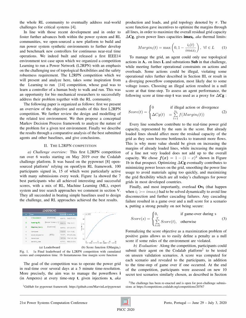
a) Challenge overview: This first L2RPN competitionran over 6 weeks starting on May 2019 over the Codalabchallenge platform. It was based on the pypownet [8] open-sourced platform1 relying on openGym RL framework. 100participants signed in, 15 of which were particularly activewith many submissions every week. Figure 1a showed the 7best participants who all achieved interesting and successfulscores, with a mix of RL, Machine Learning (ML), expertsystem and tree search approaches we comment in section V.They all succeeded in beating simple baselines used to designthe challenge, and RL approaches achieved the best results.

(a) Leaderboard (b) Score function f(Marginl)Fig. 1. 1a Final leaderboard of the L2RPN competition with cumulatedscores and computation time. 1b Instantaneous line margin score function

The goal of the competition was to operate the power gridin real-time over several days at a 5 minute time-resolution.More precisely, the aim was to manage the powerflows i(in Amperes) at every time-step t, given injections x, aka

1GitHub for pypownet framework: https://github.com/MarvinLer/pypownet

production and loads, and grid topology denoted by τ . Thescore function gave incentives to optimize the margins throughall lines, in order to maximize the overall residual grid capacity∆Cg, given power lines capacities imaxl, aka thermal limits:

Marginl(t) = max

(0, 1− il(t)

imaxl

), ∀l ∈ L (1)

To manage the grid, an agent could only use topologicalactions in Aτ on lines L and substations Sub in that challenge,while meeting further operational constraints on actions andoverloads. Some actions could be illegal, violating someoperational rules further described in Section III, or result ina diverging powerflow computation, most likely due to somevoltage issues. Choosing an illegal action resulted in a nullscore at that time-step. To assess an agent performance, thefollowing score at time-step t was used as a proxy for ∆Cg :

Score(t) =

0 if illegal action or divergence

∆Cg(t) =nl∑l=1

f(Marginl(t))(2)

Every line somehow contribute to the real-time power gridcapacity, represented by the sum in the score. But alreadyloaded lines should affect more the residual capacity of thegrid as they soon become bottlenecks to transmit more flows.This is why more value should be given on increasing themargins of already loaded lines, while increasing the marginof a line not very loaded does not add up to the overallcapacity. We chose f(x) = 1 − (1 − x)2 shown in Figure1b in that prospect. Optimizing ∆Cg eventually contributes tominimizing power losses on the grid, smoothing the power lineusage to avoid materials aging too quickly, and maximizingthe grid flexibility which are all today’s challenges for powergrids in most developed countries.

Finally, and most importantly, overload Ovl (that happenwhen il >= imaxl) had to be solved dynamically to avoid linedisconnection and further cascading failures. Any cascadingfailure resulted in a game over and a null score for a scenarios, putting a strong penalty on not being secure:

Score(s) =

0, if game-over during sT∑t=0

Score(t), otherwise(3)

Formalizing the score objective as a maximization problem ofpositive gains allows us to easily define a penalty as a nullscore if some rules of the environment are violated.

b) Evaluation: Along the competition, participants couldsubmit their agent on the Codalab platform2 to be testedon unseen validation scenarios. A score was computed foreach scenario and revealed to the participants, in additionto the time-step of game over if one occurred. At the endof the competition, participants were assessed on new 10secret test scenarios similarly chosen, as described in Section

2The challenge has been re-enacted and is open for post-challenge submis-sions at https://competitions.codalab.org/competitions/20767


PSCC 2020


https://github.com/MarvinLer/pypownet

https://competitions.codalab.org/competitions/20767

V, with no other information than their cumulative score.Finally, to reflect one main characteristic of real-time op-erations for which time is limited, resulting in a trade-offbetween exploration and exploitation, participants would onlyget a score if they managed to finish their scenario within anallocated 20-minute time budget as shown on Figure 1a. Itwas calibrated as being 10 times the running time of the mostsimple baseline: a do-nothing (DN) agent. Expert Systemsand tree-search approaches appeared to be slow, since theyrelied more extensively on simulations, and had to limit theirexploration to meet the time constraint.

c) Benefits of a Challenge: While reproducibility is a hotissue for scientific research and further model deployment,a challenge format looks appealing to avoid some pitfalls.Indeed, a challenge acts as a benchmark whose goal is todecouple the problem modeling from a solver implementation.Compared to the fine tuning of ones own method, a challengeaims at giving equal chance to every field expert to tuneits solution in a given time slot and compare against oneanother. Its success also depends on the clarity of the submittedproblem, on the ergonomy and robustness of its platform,on the transparency of its results, with an intrinsic need ofreproducibility to faithfully deliver ones score and reliablyannounce the winners. Finally, winners had to open-sourcetheir code to obtain the price, further enforcing reproducibility.

III. CHALLENGE DESIGN

The difficulty of setting up this kind of challenge lies in thefact that one has to design a whole synthetic and interactiveenvironment to test controllers (like a video game), and not justa fixed dataset. We designed it following 3 guiding principles:

1) Realism : the environment should represent real-worldpower system operational constraints and distributions.

2) Feasibility : solutions should exist to finish scenariosunder the available actions given game over conditions.

3) Interest : harder scenarios should be challenging to finishand most scenarios should be complex to optimize.

There is a natural trade-off in making a game interestingand feasible: a most interesting game will more likely be moredifficult with potential feasibility issues arising.

Now a Grid World, aka an environment for a power grid,is the combination of the following components:

• A power grid (with substations and powerlines of differ-ent characteristics) and a grid topology τ

• Real-time injections x(t), next time-step forecasts x(t+1)• Lines Capacities imaxl and additional operational rules• Events such as maintenance and contingencies

The power flows il(t) are computed by a power-flowsimulator.The platform then allows some interactions for anagent with that environment through actions aτ (t). Participantshad the option to simulate the effect of their action beforechoosing one, but using some computation time budget. Toassess how feasible and interesting an environment is foragents, we defined the following simple baseline agents :

• a “do nothing” (DN) agent that remains in the referencetopology τref and which is already robust most ofthe time, much better actually than taking random, andmostly stupid, actions.

• a single topology agent (DNτ ), which is a DN agentrunning in a constant topology τ distinct from τref .

• a greedy (GR) agent that simulate do-nothing and allunitary actions at a given time-step, and take the mostimmediately beneficial one.

These agents can finish all together most scenarios, whilehighlighting hard to complete ones. Let’s now describe in moredetails the different steps of the challenge design.

a) Choosing a Power Grid and define topology τ :To be realistic, we first chose a grid among common IEEEpower grids. For that first challenge, we chose a minimalistgrid to better ensure feasibility and help analysis, but yet agrid for which topological actions could still be useful tomanage it. Such a grid needed to be meshed with severalelectrical paths. We hence chose the IEEE14 grid as it is ameshed grid with 2 West and East corridors between a meshedSouth Transmission Grid and a meshed North DistributionGrid. Even with only 14 substations, the number of potentialoverall configurations, hence the combination of actions, istremendous. For such a size, we however did not consider theoccurrence of contingencies and maintenance since it will mostoften lead to infeasibilities. Overloads were only the result ofpeak productions or peak loads in certain areas of the grid.

The reference topology τref is the base case topology,fully meshed, with every lines in service and single electricalnode per substations. However, up to two electrical nodes arepossible per substation, modeled as a 2-bus bar.

The topology can be changed by actions aτ (t) ∈ Aτ , thatcan be of two kinds :

• Binary Line switching al (220 possible actions)• Bus bar switching of elements at a substation abusi

(220∗2+16) for 20 lines and 16 injectionsThere are as many actions as there are topology configura-

tions. Eventually, the number of reachable configurations at agiven time is limited by considering some operational rules.

Fig. 2. a) IEEE14 Grid and production localization. b) Two existing electricalcorridors between Transmission and Distribution Grids.

b) Generating Injections x(t) and Forecasts x(t+1):While the IEEE 14 grid only had initially thermal production,we introduce renewable wind and solar plants as depicted


PSCC 2020


on Figure 2 to better represents today’s energy mix anddynamics to consider managing resulting issues. The total loadconsumption profile follows the French consumption one andindividual loads are computed given a constant key factorfrom the original IEEE case on Figure 3. Solar and windpower also follow French related distribution with correlationsbetween wind and solar. The nuclear power plant is a baseload,slowly varying and the thermal power plant compensates forthe remaining production required for balancing (see Figure 3).For this challenge, we restricted the distribution of injectionsto be representative of winter months over which we observepeak loads. Next time frame forecast where also provided forinjections x with 5% gaussian noise uncertainty.

Fig. 3. a) Production, thermal and renewable, profiles over a typical monthof January. b) Load profiles, all similar modulo a proportional factor.

c) Line capacities imax and operational rules: :

Fig. 4. Number of overloads per day and hours over 50 monthly representativescenarios. Overloads mainly appear on weekdays at peak load hours or underpeak solar production around noon on the distribution grid.

The second part of the game design was about setting upthe right thermal limits (no thermal limits are given for theIEEE14 case) so that some overloads appear, not all beingeasily solvable, but many of them that can be solved by atleast a baseline to remain feasible. From the grid structureperspective, only 2 electrical corridors exists as illustrated onFigure 2. We cannot allow both of them being overloadedat the same time, since there will not exist any more pathto reroute electricity with topology to relieve all overloads.We hence chose to preferably constrain line capacities on theWest Corridor (buses 2→ 5→ 6→ 13), while keeping spatialconsistency for thermal limits overall from a grid developmentperspective. Overloads eventually appear 3% of the time overthose lines in the scenarios running DN agent. Other lines hadtheir capacities rated above the max power flow observe in thereference topology.

To make the game more interesting, we also want to have aspread distribution on the time of occurrence of overloads asshown on Figure 4. Running an ensemble of expertly selected

DNτ baselines (see Table I) solves 85% of the overloads.This demonstrates that our game is both feasible, and hassome difficult interesting situations (following our guidingprinciples). Also, the GR baseline does not perform wellon all scenarios : this agent tends to get stuck in bad localconfigurations.

Finally, real-world problems get complex because of oper-ational constraints.We choose to model the following ones:

• reaction time – time to react to an overload before theline get disconnected by protections, 2 time-steps here.

• activation time – there is a maximum number of actionsthat a human or a technology can performed in a giventime period, one action per substation here.

• recovery time (cooldown) – due to physical properties ofthe assets, there is some time after activation before aflexibility can be reactivated, set to 3 time-steps here.

You can look at flexibilities as a kind of budget. When youuse one, you consume part of your budget before recovering itsome time after. This induces some credit assignment problem.Let’s now formalize the whole problem under those settingswith the generic framework of Markov Decision Processes.

IV. PROBLEM FORMALIZATION

Markov Decision Processes (MDPs) [?] are useful and gen-eral abstractions to solve a number of problems in optimizationand control. We decide to further formalize our problem hereusing this framework, which will help determine the natureof the problem under different settings. An MDP is generallyrepresented by a tuple 〈S,A, P, r, γ〉 with:

• S the state space of observations from the environment.• A the action space, the potential agent interactions with

the environment.• P the stochastic transition function p(s(t+ 1)|s(t), a(t))

which computes the system dynamics. It defines a Marko-vian assumption.

• r(t) = r(s(t), a(t)) the immediate reward function.The policy determines the next action a(t+1) as a function

of s(t) and r(t). The policy can adapt itself (by reinforcementlearning) to maximize the expectation (over all possible tra-jectories) of this function:

G(t) =

T∑k=t+1

γk−t−1r(k) (4)

where γ ∈ [0, 1] is the discount rate.Our L2RPN problem is actually a two-factor MDP (Figure

5), a special case of MDP in which the state S is a quadruplet:• ε: unobserved influences on inputs x.• x: observed inputs of the system, not influenced by the

actions of the agent.• τ : other observed inputs of the system, influenced by the

actions of the agent.• y: observed outputs of the system, y = F (x, τ ).Function F specifies the system of interest and y is essen-

tially here powerflows il and overloads Ovl. F is a function of


PSCC 2020


two factors x and τ (injections and topology in our case). The‘observed inputs’ x may or may not be organized in a timeseries. In our case they are. Injections are continuous time-series. For τ , it is only changing under limited agent actionsand some rare events such as contingencies and maintenance.

The agent’s actions only influence τ . Although there aremany ways in which τ (t);x(t); y(t) could influence (t+1)variables, we only considered the following:

• x→ x: injections are timeseries.• τ → τ : agent’s ”position” τ (t + 1) is constrained by

past positions τ (t) given the limited action rule, de factolimiting the freedom of the agent to influence y.

• y → τ : overloaded flows can lead to line disconnections,or cascading failure, hence influencing the topology .

• τ → a: recovery time constrains future actions.

Without operational constraints and robustness considera-tion of cascading failures, the problem is mostly an instanceof the contextual bandit more specific case on Figure 5 (onlyx(t)→ x(t+1)) under which more specific algorithm than RLcan be preferred and perform quite well. Adding τ → τ bylimiting instantaneous actions makes it a regular RL problem.Our platform could actually run this latter setting as an easymode to make an agent’s training easier at first. Howeverthe problem we proposed in this first challenge, our hardmode, already involved some more complexity as depicted onFigure 5. Successful approaches in the easy mode would notnecessarily work in the hard mode, especially since it involvesrobustness issues in the latter case.

Fig. 5. a) Contextual Bandit framework. b) L2RPN MDP formalization.

These causal diagrams are hence useful for understandingthe problem proposed. It helps the designer anticipate if mod-eling a new constraint will change the nature and complexity ofthe problem and it helps the participant select the appropriateclass of methods to solve it. In particular, ML and RL methodsindeed appeared suited for this first challenge as expected.

V. RESULT ANALYSIS

We now review the challenge results, by first describingthe properties of the scenarios on which participants weretested, and giving a description of the best agents. Then weanalyze the agents behavior on these and eventually present apost-analysis of their performance. Finally we will propose an

oracle approach to derive a near upper-bound for the scores,to better assess the optimization gap of the agents.

a) Validation and test scenarios: In order to select in-teresting scenarios, we tried to combine multiple criteria thatwere identically set for both validation and test scenarios:

• Difficulty levels: difficulty ranges from easy (no overloadat all for the DN agent) to hard (no known solution hasbeen found using our ensemble of DNτ agent baseline).It reduces the likeliness of having tie contestants.

• Diverse tasks: some scenarios focus on handling over-loads in the morning, while others test evening peakconsumption management. In a scenario, no overloadappears, to test agents does not react randomly. In others,overloads vanish naturally, to test agents do not overreact.

• Diverse context: we include variability by changing theday of the week of the scenarios, to make sure thepowergrid can be handled for all days of the week, andnot only at some very restrictive times.

• Diverse horizons: we finally have scenarios of differentlength, varying from 1 day (288 time-steps) to 3 days (864time-steps), to test agents in different kind of settings:longer scenarios favor stable agents with longer horizon,shorter scenarios favor greedy agents.

Those scenarios were mainly selected to test the robustnessof agents, that is their ability to finish a given scenario. How-ever, beside being robust, participants still had to continuouslyoptimize the grid margins. Let’s now describe the best agentsand examine their behavior on the test scenarios.

b) Agent Description: From Figure 1a, we can see thatonly the groups called “Lebron James” (LB), “LearningRL”(LR) and “Stephan Curry” (2nd team from Geirina, so we onlyconsider LB) managed to finish all test scenarios, with ML +RL approaches. Both codes are open-source and referenced onthe challenge website 3. “Kamikaze” (KM, ML approach) and“Smart Dispatcher” (SD, Expert system + greedy validation)each failed on one, whereas they previously managed allvalidation scenarios. “Menardpr” (MD, greedy tree searchapproach) failed on one, on both test and validation scenarios.Winners were less computationally intensive at test time,thanks to Machine Learning, while also being more effcicient,making them relevant in a setting of real-time decision making.

Comparing LB and LR from a code analysis, LR appearedto be the only participant to never query the simulate functionto validate or explore additional actions at test time: this isquite an achievement to only rely on what the agent learnt, andtrust it. Its model was based on the actor critic (A3C) algorithm[11]. This is an architecture with two main components, apolicy network (actor) and a value network (critic). A3Caim at learning a policy function directly, through the actormodule. The critic module then criticize the actor given thenew state value after taking an action, to adjust and improve itsbehavior. Actor and critic modules are learnt asynchronouslyby pooling multiple workers that learn independently andimprove a global agent.

3Benchmark competition & github of winners at l2rpn.chalearn.org


PSCC 2020


l2rpn.chalearn.org

LB agent on the other hand combined an RL model basedon a dueling DQN algorithm [17], coupled to a set of actionsselected through extended prior analysis and imitation learn-ing. Dueling DQN is most similar to DQN [10] except that theneural network architecture explicitly try to encode separatelyat its core a state value function and an action advantagefunction, later combined to better estimate the Q-value.

In addition, LB uses few expert rules, especially ”don’tdo anything if all your margins are good enough, below athreshold of 80%”, and make extensive use of the simulatefunction when deciding on taking an action, to stronglyvalidate a set of suggested action. This is representative onhow operators have been doing until today. Their approach iscloser to an assistant: an RL model suggests some actions andan expert model make a cautious choice among them and theones he knows, validating with a simulator.

Fig. 6. Number of actions used at different substations (red) or lines (blue),ordered by indices, for different agents and our oracle over test scenarios.

c) Agents action space: All participants tried with dif-ferent strategies to reduce the action space to explore atfirst. SD relied on its operator’s expertise to identify relevantsubstations and lines to test on, still using a diverse set of assetswith selected topologies. MD only focused on line switchingto meet the time constraint with a tree search approach.However, most participants let aside line switching, sometimesan interesting option when no overloads exist to reroute someflows, but often detrimental when the grid is overloaded.

LR also used some domain knowledge over the symme-tries in a substation to reduce the number of true actions.More interestingly, they started their exploration from scratchand learnt robust actions automatically through a curriculumlearning. They indeed started to learn in an easy mode (nogame over), upsampling the scenarios to quickly see morediverse situations. They somehow already learnt useless ac-tions and potentially useful actions to route the flows. Theythen switched to the hard mode with the appropriate timeresolution to learn managing overloads and being robust tothem. They used their own reward function when learning topenalize strongly on overloads when occurring, different fromour score in (2). Our score is not a good reward functionto learn from in that prospect, as its gradient, and hence thelearning signal, is null in the overload regime. They eventuallyconverged to only act on two substations, a bit restrictive. Thismight be changed by relaxing their reward function.

Fig. 7. Agent behavior over validation scenario 3 showing the depth of agentactions at a given time-step, 0 meaning the agent is in the reference topology

LB team on the other hand did an extensive analysis oninfluential topologies on a batch of sampled grid states toinitialize their learning. At the end, they used quite a diverseset of assets. Figure 6 summarizes the number and diversityof actions agents used on test scenarios.

d) Behavior analysis : Looking at agent actions in real-time from Figure 7 on a test scenario, we can detect differentkinds of behavior. SD is indeed doing lots of actions, tryingto optimize the score continuously, but somehow going backand forth erratically when the grid is loaded: overloads mightbe appearing due to its actions. LB is a pretty stable agent,anticipating soon enough potential overloads through its expertrule. However its topology seems to always be drifting fromthe reference topology which might be detrimental on longscenarios. Finally, LR is also quite stable due to its small actionspace but has the ability to go back and forth. Extended AIagent behavior analysis will be conducted in future works, asit is an emerging field [13] with new tools being released [12].

We eventually ran an additional post analysis experiment onlarger batch of monthly scenarios given for training. It showedthat all agents are still failing on several scenarios (LB: 5 fails,LR: 11 fails, SD: 9 fails), highlighting some instabilities on thelong term. Scenario 37 appeared especially difficult with noagent succeeding. We should hence aposteriori adjust or aug-ment our selection criteria to develop a more comprehensivebenchmark of this task. Also, beyond robustness, the challengewas also about continuously optimizing the flows on the grid.

e) Revised scores with oracle baseline: In the shortduration of the competition, participants mainly focused ontheir agent robustness, as a single gameover prevented themfrom winning. From the behavior analysis, agents do notappear to take many actions over a scenario, except from SDagent, which might indicate that agents did not try to optimizethe flows beside avoiding overloads. To assess how good theydid on this second task, we need to define an upper-boundbaseline to get a better idea of what a good score should be.

While imperfect information is given to the participantsalong the game as they don’t know yet the future, as organizerswe can make use of the full scenario information to computean oracle baseline, our upper-bound. For our method, we relyon the connection there exists between topology configuration


PSCC 2020


r(0, 0)

r(1, 0)

r(2, 0)

r(3, 0)

r(0, 1)

r(1, 1)

r(2, 1)

r(3, 1)

r(0, 2)

r(1, 2)

r(2, 2)

r(3, 2)

r(0, 3)

r(1, 3)

r(2, 3)

r(3, 3)

r(0, 4)

r(1, 4)

r(2, 4)

r(3, 4)

r(0, 5)

r(1, 5)

r(2, 5)

r(3, 5)

t0 t1 t2 t3 t4 t5 t6time

τ0

τ1

τ2

τ3

r(1, 0) r(1, 1) r(1, 2)

r(2, 3)

r(3, 4) r(3, 5)

r(2, 3)

r(3, 3)

Fig. 8. reward graph G for several topology configurations τ and allowedtransitions in dashed green. The oracle optimal path (in red) misses a maximmediate reward at t3 as no direct transition is allowed between τ1 and τ3.

and topological action: given one action we can deduce thetopology configuration we reach, knowing which configurationto reach to get some reward we can deduce the necessaryaction. We decided to run test scenarios under thousands oftopology configurations in parallel (not all, which is too hardcomputationally) to later identify what would have been verygood topologies at a given time and infer the preferred courseof actions. Ultimately, it is framed as a longest path problemas on Figure 8. Our method can be decomposed in 5 steps:

1) Define a dictionary of interesting unitary actions Da

from n unitary selected assets as on Table I2) Identify all combinations of Da actions to create the

oracle action space Aoracle and related topology con-figuration space S(τ)oracle when applied to τref . Atopology can be n action away from the reference one.

3) Apply all τ ∈ S(τ)oracle independently and run themin parallel on scenarios to compute the reward of eachconfiguration τ at each time-step t. This results indirected chains Gτ with edges eGτ (t) = reward(τ, t)

4) From all {Gτ}, build the overall connex graph G of pos-sible topology trajectories, given allowed topology tran-sitions from operational rule. Add edges between reach-able configurations (τa,τb): e(τa,τb)(t) = reward(τb, t).

5) Compute the best score through the longest path onthe directed acyclic graph G and determine the relatedcourse of actions {a(t)}t=0..T ∈ Aoracle.

Our score is always greater than all agents while respectingthe operational rules, effectively defining on upper-bound. Todetermine how good other agents did, we define a revised scoretaking DN as a zero-reference score (computed in easy modeconsidering the optimization task only), oracle as a max:

ScoreNormalized =Scoreagent − ScoreDNScoreoracle − ScoreDN

(5)

The revised scores in Table I suggest that there still exists a gapbetween our oracle upper-bound and the best submitted agents.Figure 6 highlights that our oracle continuously took someactions, every 2 to 3 timesteps on average, as opposed to otheragents. This confirms that agents did not do quite well on thisoptimizing task. Thus we reopened the challenge test case as a

Felxibility id Target config.

Sub 6 1 [0, 0, 0, 0, 1, 1]2 [0, 1, 0, 0, 1, 1]

Sub 5 1 [0, 1, 0, 0, 1]2 [0, 0, 1, 0, 1]

Sub 4

1 [0, 0, 1, 0, 1, 0]2 [0, 0, 0, 1, 1, 0]3 [1, 0, 1, 0, 1, 1]4 [1, 0, 1, 0, 1, 0]

Sub 91 [1, 0, 1, 0, 1]2 [0, 0, 1, 0, 1]3 [1, 1, 0, 1, 1]

Sub 2 1 [1, 1, 0, 1, 0, 1]2 [1, 1, 0, 1, 0, 0]

Lines 2-4, 5-610-11, 13-14

0 [0]1 [1]

(a) Selected unitary actions at subs andlines for oracle. In bold, the ones usedprevisously for thermal limit design

Scenario SD LB1 72,5 61,52 -10,5 90,23 53 82,54 49,5 81,55 47,5 70,06 48 477 19,5 638 39,5 77,59 52,5 9310 56,5 56,5

(b) Normalized scores for SD and LBagents, compared to an oracle with100 points. There still exists an op-timization gap to improve on.

TABLE I

benchmark3. This highlights that controlling the topology stillremains a hard problem given a huge action space requiringlots of exploration. It also challenges us as organizers to offermore representative scores that will give more incentives tothe participants to perform better on a related task.

VI. CONCLUSIONS

The challenge was successful in addressing safety consider-ations and was necessary to open a new research avenue for abroad community, extended to Machine Learning researchers.It demonstrated that developing topological controllers forreal-time decision making is indeed possible, especially whenusing reinforcement learning. Framing the problem as a two-factor MDP allowed us to also expose the difficulties facedby reinforcement learning solutions to such control problems.The diversity of submissions and behaviors helped us ap-preciate the pros and cons of each approach. Evaluating theparticipants’ performance pushed us to define new interestingbaselines and scoring metrics for future research and challengedesigns. Our post-challenge analyses revealed both the feasi-bility of such approaches and the important gap to optimality,particularly for continuous power flow optimization, giving usan incentive to take the design of a new benchmark to the nextlevel, including scaling up the dimensions of the grid.

Acknowledgements

Many people have contributed to the design and implementation of theL2RPN challenge. We would like to acknowledge the contributions of MarcMozgawa, Kimang Khun, Joao Arajo, Marc Schoenauer, Patrick Panciatici,Olivier Pietquin, and Gabriel Dulac-Arnold. The challenge is running on theCodalab platform, administered by Universit Paris-Saclay and maintained byCKCollab LLC, with primary developers Eric Carmichael and Tyler Thomas

REFERENCES

[1] R. Bacher and H. Glavitsch. Network topology optimization withsecurity constraints. IEEE Trans. Power Syst., vol. 1, no. 4, 1986.

[2] N. Brown and T. Sandholm. Safe and nested subgame solving forimperfect-information games. NIPS, 2017.

[3] B. Donnot, I. Guyon, and al. Anticipating contingencies in power gridsusing fast neural net screening. IEEE WCCI, 2018.


PSCC 2020


[4] G. Dulac and al. Challenges for real-world reinforcement learning. 2019.[5] F. M. Fisher E., O’Neill R. Optimal branch switching. IEEE Transac-

tions on Power Systems, 2008.[6] S. M. G Dalal, E Gilboa. Hierarchical decision making in electricity

grid management. ICML, 2016.[7] M. Glavic, R. Fonteneau, and D. Ernst. Reinforcement learning for

electric power system decision and control: Past considerations andperspective. WCIFAC, 2017.

[8] M. Lerousseau. pypownet: A modular python library for reinforcementlearning on power systems management. in review for jmlr-oss.

[9] A. Marot and al. Expert system for topological remedial action discoveryin smart grids. Medpower, 2018.

[10] V. Mnih and al. Human-level control through deep reinforcementlearning. Nature, 518(7540):529–533, 2015.

[11] V. Mnih, A. P. Badia, and al. Asynchronous methods for deepreinforcement learning. CoRR, abs/1602.01783, 2016.

[12] I. Osband and al. Behaviour suite for reinforcement learning. 2019.[13] I. Rahwan and al. Machine behaviour. Nature, 2019.[14] K. S. and al. Learning to run challenge: Synthesizing physiologically

accurate motion using deep reinforcement learning. 2018.[15] D. Silver and al. Mastering the game of go with deep neural networks

and tree search. Nature 529, 2016.[16] R. S. Sutton and A. G. Barto. Reinforcement learning: An introduction.

MIT press, 2018.[17] Z. Wang, N. de Freitas, and M. Lanctot. Dueling network architectures

for deep reinforcement learning. CoRR, abs/1511.06581, 2015.


PSCC 2020


learning to run a power network challenge for training

Documents