learning to grasp unknown objects using weighted random
TRANSCRIPT

University of Central Florida University of Central Florida
STARS STARS
Electronic Theses and Dissertations, 2004-2019
2014
Learning to Grasp Unknown Objects using Weighted Random Learning to Grasp Unknown Objects using Weighted Random
Forest Algorithm from Selective Image and Point Cloud Feature Forest Algorithm from Selective Image and Point Cloud Feature
Md Shahriar Iqbal University of Central Florida
Part of the Electrical and Electronics Commons
Find similar works at: https://stars.library.ucf.edu/etd
University of Central Florida Libraries http://library.ucf.edu
This Masters Thesis (Open Access) is brought to you for free and open access by STARS. It has been accepted for
inclusion in Electronic Theses and Dissertations, 2004-2019 by an authorized administrator of STARS. For more
information, please contact [email protected].
STARS Citation STARS Citation Iqbal, Md Shahriar, "Learning to Grasp Unknown Objects using Weighted Random Forest Algorithm from Selective Image and Point Cloud Feature" (2014). Electronic Theses and Dissertations, 2004-2019. 4790. https://stars.library.ucf.edu/etd/4790
LEARNING TO GRASP UNKNOWN OBJECTS USING
WEIGHTED RANDOM FOREST ALGORITHM FROM
SELECTIVE IMAGE AND POINT CLOUD FEATURE
by
MD. SHAHRIAR IQBAL
B.Sc. University of Dhaka, 2011
A thesis submitted for the partial fulfillment of the requirements
for the degree of Master of Science
in the Department of Electrical Engineering and Computer Science
in the College of Engineering and Computer Science
at the University of Central Florida
Orlando, Florida
Fall Term
2014
Major Professor: Aman Behal

ii
© 2014 Md. Shahriar Iqbal

iii
ABSTRACT
This method demonstrates an approach to determine the best grasping location on an unknown
object using Weighted Random Forest Algorithm. It used RGB-D value of an object as input to
find a suitable rectangular grasping region as the output. To accomplish this task, it uses a
subspace of most important features from a very high dimensional extensive feature space that
contains both image and point cloud features. Usage of most important features in the grasping
algorithm has enabled the system to be computationally very fast while preserving maximum
information gain. In this approach, the Random Forest operates using optimum parameters e.g.
Number of Trees, Number of Features at each node, Information Gain Criteria etc. ensures
optimization in learning, with highest possible accuracy in minimum time in an advanced
practical setting. The Weighted Random Forest chosen over Support Vector Machine (SVM),
Decision Tree and Adaboost for implementation of the grasping system outperforms the stated
machine learning algorithms both in training and testing accuracy and other performance
estimates. The Grasping System utilizing learning from a score function detects the rectangular
grasping region after selecting the top rectangle that has the largest score. The system is
implemented and tested in a Baxter Research Robot with Parallel Plate Gripper in action.

iv
ACKNOWLEDGMENTS
I would like to express my deepest and sincere gratitude to my advisor, Dr. Aman Behal.
Without his patience, guidance, and support this research would not have been possible, nor
would I have been capable of completing it. The learnings I have received from him are
immense. I will always have a proud story to tell everyone that I happened to work under his
knowledgeable supervision. In addition, Dr. Michael G. Haralambous, has also been an
invaluable resource and a source of guidance and inspiration throughout this work. I would also
like to thank Dr. Lotzi Boloni, who was instrumental in helping assist in the machine learning
aspects of this project. A special thank you to my research colleagues who have helped me
achieve all that I have thus far with their help and support: Nicholas Paperno, Amirhossain
Jabalemi, Kun Zhang and Shahriar Talebi. I would like to thank Mahmudur Rahman
Chowdhury, Fahad Abdullah, Md. Mokarram Hossain, Md. Towhidul Islam, Tahrim Alam, Md.
Rakibul Islam, Md. Zihad Tarafdar, A. K. M. Bodiuzzaman, Md. Ariful Hossain, Sakif Ahsan, M
Shamim Rahman, Md. Nasir Uddin, Raihan Abir, Golam Mohiuddin, Towfiq Rahman and
Kamrul Islam who helped and supported me along the way. Finally, thanks to my parents, my
sister, my nieces and Iffath Mizan for all of the sacrifices they have done and the encouragement
they have provided over the years in furthering my education and providing a mountain of
support that has allowed me to accomplish this goal.

v
TABLE OF CONTENTS
LIST OF FIGURES ....................................................................................................................... ix
LIST OF TABLES ....................................................................................................................... xiii
CHAPTER 1 : INTRODUCTION .................................................................................................. 1
1.1 Robotic Grasping.............................................................................................................. 1
1.2 Application and Impact .................................................................................................... 2
1.3 Problem Statement ........................................................................................................... 3
1.3.1 Rectangle as a Grasping Region ............................................................................... 3
1.3.2 Goal ........................................................................................................................... 4
1.4 Contribution of the Thesis ................................................................................................ 5
1.5 Organization of the Thesis ............................................................................................... 5
1.6 References ........................................................................................................................ 8
CHAPTER 2 : BACKGROUND AND RELATED WORK .......................................................... 9
2.1 Introduction ...................................................................................................................... 9
2.2 Chapter Objectives ........................................................................................................... 9
2.3 Analytical Approaches ..................................................................................................... 9
2.3.1 Force Closure Grasps .............................................................................................. 10
2.3.2 Task Compatibility.................................................................................................. 11
2.4 Empirical Approaches .................................................................................................... 12
2.4.1 Systems based on human observation..................................................................... 12
2.4.2 Systems based on object observation ...................................................................... 13
2.5 Discussion ...................................................................................................................... 14
2.6 References ...................................................................................................................... 14
CHAPTER 3 : FEATURES USED AND EXTRACTION TECHNIQUE .................................. 20
3.1 Introduction .................................................................................................................... 20
3.1.1 Feature Extraction ................................................................................................... 20
3.2 Chapter Objectives ......................................................................................................... 21
3.2.1 Image Feature Extraction Technique ...................................................................... 22
3.2.2 Non-linear Image Feature Extraction Technique .................................................... 27
vi
3.2.3 Point Cloud Feature Extraction Technique ............................................................. 29
3.2.4 Non-linear Point Cloud Feature Extraction Technique .......................................... 32
3.2.5 Fast Point Feature Histogram Descriptors Extraction Technique........................... 34
3.2.6 Geometric Feature Extraction Technique ............................................................... 36
3.3 Discussion ...................................................................................................................... 36
3.4 References: ..................................................................................................................... 36
CHAPTER 4 : WHY RANDOM FOREST? ................................................................................ 38
4.1 Introduction .................................................................................................................... 38
4.1.1 Cross Validation Score ........................................................................................... 39
4.1.2 Precision .................................................................................................................. 40
4.1.3 Recall ...................................................................................................................... 40
4.1.4 Accuracy ................................................................................................................. 40
4.1.5 F1 Score .................................................................................................................. 41
4.1.6 ROC Score .............................................................................................................. 41
4.2 Chapter Objectives ......................................................................................................... 42
4.3 Definition of Performance Metric .................................................................................. 42
4.4 Support Vector Machine ................................................................................................ 43
4.4.1 SVM with Linear kernel ......................................................................................... 44
4.4.2 Parameters used in SVM with linear kernel and Results ........................................ 45
4.4.3 SVM with Polynomial kernel ................................................................................. 46
4.4.4 Parameters used in SVM with Polynomial kernel and Results............................... 46
4.4.5 SVM with Radial Basis Function kernel ................................................................ 47
4.4.6 Parameters used in SVM with Radial Basis Function kernel and Results .............. 47
4.4.7 Comparison of Error Estimates from Linear, Polynomial and RBF SVM and
Discussion .............................................................................................................................. 48
4.4.8 Evaluation Metric Results from Linear, Polynomial and RBF SVM ..................... 48
4.5 Information Gain Parameter Definition for Tree based Learning Algorithms............... 49
4.5.1 Gini Impurity .......................................................................................................... 49
4.5.2 Entropy .................................................................................................................... 50
4.6 Decision Tree Algorithm ................................................................................................ 50
4.6.1 Parameters used in Decision Tree Algorithm ......................................................... 50

vii
4.6.2 Comparison of Error Estimates using Decision Tree Algorithm with different
Parameters ............................................................................................................................. 54
4.6.3 Performance Metric Results from Decision Tree Algorithms ................................ 55
4.7 Adaboost Algorithm ....................................................................................................... 56
4.7.1 Parameters used in Adaboost Algorithm ................................................................ 56
4.7.2 Error Estimates from Adaboost Algorithm ............................................................. 60
4.7.3 Performance Metric Results on Adaboost Algorithm ............................................. 61
4.8 Random Forest Algorithm .............................................................................................. 62
4.9 Evaluation of Dataset to select range of Number of Trees ............................................ 62
4.9.1 Weighted random Forest Algorithm used in this Method ...................................... 63
4.9.2 Parameters used in Random Forest Algorithm ....................................................... 64
4.9.3 Error Estimate Results from Random Forest Algorithm using Gini....................... 64
4.9.4 Error Estimate Results from Random Forest Algorithm using Entropy Criteria.... 71
4.9.5 Performance Metric Results from Random Forest Algorithm with Different
Number of Trees .................................................................................................................... 79
4.10 Selection of the Best Algorithm with Optimal Parameters ............................................ 84
4.11 Selection of Most Significant Features .......................................................................... 85
4.12 References ...................................................................................................................... 87
CHAPTER 5 : GRASPING ALGORITHM ................................................................................. 89
5.1 Introduction .................................................................................................................... 89
5.2 Chapter Objectives ......................................................................................................... 91
5.3 Learning a Score Function ............................................................................................. 91
5.3.1 Definition of a Score Function ................................................................................ 91
5.3.2 Computing of a Score Function .............................................................................. 92
5.3.3 Assumption ............................................................................................................. 93
5.3.4 Incremental Search Procedure ................................................................................ 94
5.4 Background Subtraction using Mixture of Gaussian Model .......................................... 95
5.5 Algorithm ....................................................................................................................... 98
5.6 Hardware Setup .............................................................................................................. 99
5.7 Evaluation Metric ........................................................................................................... 99
5.7.1 Point Metric .......................................................................................................... 100

viii
5.7.2 Rectangle Metric ................................................................................................... 100
5.8 Experimental Results.................................................................................................... 101
5.9 Training Dataset ........................................................................................................... 101
5.10 Testing Results ............................................................................................................. 102
5.11 Discussion .................................................................................................................... 105
5.12 References .................................................................................................................... 107
CHAPTER 6 : CONCLUSION AND FUTURE SCOPE OF RESEARCH ............................... 109
6.1 Introduction .................................................................................................................. 109
6.2 Chapter Objectives ....................................................................................................... 109
6.3 Summary of the Grasping System ................................................................................ 109
6.4 Innovations in this Method ........................................................................................... 111
6.5 Scope of Further Research ........................................................................................... 111
6.6 References .................................................................................................................... 112
APPENDIX A: FORCE CLOSURE GRASP ............................................................................. 113
APPENDIX B: FAST POINT FEATURE HISTOGRAM DESCRIPTORS ............................. 115
Appendix B: References.......................................................................................................... 116

ix
LIST OF FIGURES
Figure 1-1 Rectangle as a Grasping Region ................................................................................... 3
Figure 1-2 Goal of the method is to find a rectangle on object from 2-D image and Point Cloud
Data .......................................................................................................................................... 4
Figure 1-3 Organization of the Thesis ............................................................................................ 7
Figure 3-1: Features are extracted from subdividing the rectangle into Top, Middle and Bottom
Horizontal strips. ................................................................................................................... 20
Figure 3-2 Total Number of Features in this Method ................................................................... 21
Figure 3-3: Image Feature Extraction Technique ......................................................................... 23
Figure 3-4 Color Features Extracted from (left) Positive Rectangles (right) Negative Rectangles
............................................................................................................................................... 24
Figure 3-5 Filter used for Texture Feature Extraction .................................................................. 24
Figure 3-6 Texture Feature Extraction Technique ........................................................................ 25
Figure 3-7 Texture Features Extracted from (left) Positive Rectangles (right) Negative
Rectangles .............................................................................................................................. 25
Figure 3-8 Filters used to extract Edge Features .......................................................................... 26
Figure 3-9 Edge Feature Extraction Technique ............................................................................ 26
Figure 3-10 Texture Feature Extracted from (left) Positive and (right) Negative Examples ....... 27
Figure 3-11Nonlinear Color Features Extracted from (left) Positive Rectangles (right) Negative
Rectangles .............................................................................................................................. 28
Figure 3-12 Nonlinear Texture Features Extracted from (left) Positive Rectangles (right)
Negative Rectangles .............................................................................................................. 28
Figure 3-13 Nonlinear Edge Features Extracted from (left) Positive Rectangles (right) Negative
Rectangles .............................................................................................................................. 29
Figure 3-14 Depth Feature Extraction from (left) Positive Rectangles (right) Negative Rectangles
............................................................................................................................................... 30
Figure 3-15 Surface Normal Features Extracted from (left) Positive Rectangles (right) Negative
Rectangles .............................................................................................................................. 31
Figure 3-16 Surface Curvature Features Extracted from (left) Positive Rectangles (right)
Negative Rectangles .............................................................................................................. 31
Figure 3-17 Non-linear Depth Features Extracted from (left) Positive Rectangles (right) Negative
Rectangles .............................................................................................................................. 32
Figure 3-18 Non-linear Surface Normal Features Extracted from (left) Positive Rectangles (right)
Negative Rectangles .............................................................................................................. 33
Figure 3-19 Non-linear Surface Normal Features Extracted from (left) Positive Rectangles (right)
Negative Rectangles .............................................................................................................. 34
Figure 3-20 Viewpoint Feature Histogram Descriptors from (left) Positive Examples (right)
Negative Examples ................................................................................................................ 35
Figure 4-1Confusion Matrix and ROC Curve of Linear SVM ..................................................... 45
x
Figure 4-2 Confusion Matrix and ROC Curve of Polynomial SVM ............................................ 46
Figure 4-3 Confusion Matrix and ROC Curve of RBF SVM ....................................................... 47
Figure 4-4 Evaluation Metric Results for Linear, Polynomial and RBF SVM ............................ 49
Figure 4-5 Confusion Matrix and ROC Curve for Decision Tree Gini using 2110 features at each
node ....................................................................................................................................... 51
Figure 4-6 Confusion Matrix and ROC Curve for Decision Tree Gini using 46 features at each
node ....................................................................................................................................... 51
Figure 4-7 Confusion Matrix and ROC Curve for Decision Tree Gini using 11 features at each
node ....................................................................................................................................... 52
Figure 4-8 Confusion Matrix and ROC Curve of Decision Tree Entropy using 2110 features at
each node ............................................................................................................................... 52
Figure 4-9 Confusion Matrix and ROC Curve of Decision Tree Entropy using 46 features at each
node ....................................................................................................................................... 53
Figure 4-10 Confusion Matrix and ROC curve of Decision Tree Entropy using 11 features at
each node ............................................................................................................................... 53
Figure 4-11 Performance Metric Results for Decision Tree Algorithm using Different Criteria 55
Figure 4-12 Confusion Matrix and ROC Curve using Adaboost with 32 base estimators ........... 57
Figure 4-13 Confusion Matrix and ROC curve using Adaboost with 64 base estimators ............ 57
Figure 4-14 Confusion Matrix and ROC Curve using Adaboost with 128 base estimators ......... 58
Figure 4-15 Confusion Matrix and ROC Curve using Adaboost with 256 base estimators ......... 58
Figure 4-16 Confusion Matrix and ROC Curve using Adaboost with 512 base estimators ......... 59
Figure 4-17 Confusion Matrix and ROC Curve using Adaboost with 1024 base estimators ....... 59
Figure 4-18 Performance Metric Result for Adaboost Algorithm using different Base Estimators
............................................................................................................................................... 61
Figure 4-19 Confusion Matrix and ROC Curve of Random Forest Gini using 32 Trees and 46
features at each node .............................................................................................................. 64
Figure 4-20 Confusion Matrix and ROC Curve using Random Forest Gini using 32 Trees and 11
features at each node .............................................................................................................. 65
Figure 4-21 Confusion Matrix and ROC Curve using Random Forest Gini using 64 Trees and 46
features at each node .............................................................................................................. 65
Figure 4-22Confusion Matrix and ROC Curve using Random Forest Gini using 64 Trees and 11
features at each node .............................................................................................................. 66
Figure 4-23 Confusion Matrix and ROC Curve using Random Forest Gini using 128 Trees and
46 features at each node ......................................................................................................... 66
Figure 4-24 Confusion Matrix and ROC Curve using Random Forest Gini using 128 Trees and
11 features at each node ......................................................................................................... 67
Figure 4-25 Confusion Matrix and ROC Curve using Random Forest Gini using 256 Trees and
46 features at each node ......................................................................................................... 67
Figure 4-26 Confusion Matrix and ROC Curve using Random Forest Gini using 256 Trees and
11 features at each node ......................................................................................................... 68

xi
Figure 4-27 Confusion Matrix and ROC Curve using Random Forest Gini using 512 Trees and
46 features at each node ......................................................................................................... 68
Figure 4-28 Confusion Matrix and ROC Curve using Random Forest Gini using 512 Trees and
11 features at each node ......................................................................................................... 69
Figure 4-29 Confusion Matrix and ROC Curve using Random Forest Gini using 1024 Trees and
46 features at each node ......................................................................................................... 69
Figure 4-30 Confusion Matrix and ROC Curve using Random Forest Gini using 1024 Trees and
11 features at each node ......................................................................................................... 70
Figure 4-31 Confusion Matrix and ROC Curve of Random Forest Entropy with 32 trees using 46
features at each node .............................................................................................................. 72
Figure 4-32 Confusion Matrix and ROC Curve of Random Forest Entropy with 32 trees using 11
features at each node .............................................................................................................. 72
Figure 4-33 Confusion Matrix and ROC Curve of Random Forest Entropy with 64 trees using 46
features at each node .............................................................................................................. 73
Figure 4-34 Confusion Matrix and ROC Curve of Random Forest Entropy with 64 trees using 11
features at each node .............................................................................................................. 73
Figure 4-35 Confusion Matrix and ROC Curve of Random Forest Entropy with 128 trees using
46 features at each node ......................................................................................................... 74
Figure 4-36 Confusion Matrix and ROC Curve of Random Forest Entropy with 128 trees using
11 features at each node ......................................................................................................... 74
Figure 4-37 Confusion Matrix and ROC Curve of Random Forest Entropy with 256 trees using
46 features at each node ......................................................................................................... 75
Figure 4-38 Confusion Matrix and ROC Curve of Random Forest Entropy with 256 trees using
11 features at each node ......................................................................................................... 75
Figure 4-39 Confusion Matrix and ROC Curve of Random Forest Entropy with 512 trees using
46 features at each node ......................................................................................................... 76
Figure 4-40 Confusion Matrix and ROC Curve of Random Forest Entropy with 512 trees using
11 features at each node ......................................................................................................... 76
Figure 4-41 Confusion Matrix and ROC Curve of Random Forest Entropy with 1024 trees using
46 features at each node ......................................................................................................... 77
Figure 4-42 Confusion Matrix and ROC Curve of Random Forest Entropy with 1024 trees using
11 features at each node ......................................................................................................... 77
Figure 4-43Comparison of Performance Metric Results of Random Forest Algorithm using 32
Trees ...................................................................................................................................... 79
Figure 4-44 Comparison of Performance Metric Results of Random Forest Algorithm using 64
Tree ........................................................................................................................................ 80
Figure 4-45 Comparison of Performance Metric Results of Random Forest Algorithm using 128
Trees ...................................................................................................................................... 81
Figure 4-46 Comparison of Performance Metric Results of Random Forest Algorithm using 256
Trees ...................................................................................................................................... 82
xii
Figure 4-47 Comparison of Performance Metric Results of Random Forest Algorithm using 512
Trees ...................................................................................................................................... 83
Figure 4-48 Comparison of Performance Metric Results of Random Forest Algorithm using 1024
Trees ...................................................................................................................................... 84
Figure 4-49 Important Variable Selection Algorithm ................................................................... 86
Figure 5-1 Incremental Fast Search Algorithm Used in this System............................................ 95
Figure 5-2 Background Subtraction result using Mixture of Gaussian subtraction Algorithm. The
top left image is background, the one on the right is the image of the object and the bottom
image illustrates the foreground mask after subtracting the background from the foreground
............................................................................................................................................... 97
Figure 5-3 Algorithm used for Finding Best Grasping Rectangle ................................................ 98
Figure 5-4 Screenshot of Some Objects of Cornell University Personal Robotics Dataset from
Personal Robotics Website used for Training ..................................................................... 101
Figure 5-5 Grasping Rectangles on Computational Control Systems Laboratory University of
Central Florida Dataset (From top left clockwise: Can, Holder, Tea, Window Cleaner, Soap
(orientation 1), Soap (orientation 2), Toothpaste and Remote) ........................................... 102
Figure 5-6 Unsuccessful grasping result on multimeter ............................................................. 106
Figure 5-7 Unsuccessful grasping result on a Penholder ............................................................ 106

xiii
LIST OF TABLES
Table 4-1Comparison of Error Estimates from Linear, Polynomial and RBF SVM.................... 48
Table 4-2 Error Estimates of Decision Tree Algorithm using different Parameters .................... 54
Table 4-3 Error Estimates from Adaboost Algorithm using different Base Estimators ............... 60
Table 4-4 Error Estimates obtained for different parameters of Random Forest Algorithm using
Gini Criteria ........................................................................................................................... 71
Table 4-5 Error Parameters obtained for different parameters of Random Forest Algorithm using
Entropy Criteria ..................................................................................................................... 78
Table 4-6 Selection of Best Algorithm with Optimal Parameters ................................................ 85
Table 5-1 Result on Cornell University Dataset ......................................................................... 103
Table 5-2 Result on Computational Control System Laboratory University of Central Florida
Dataset ................................................................................................................................. 104

1
CHAPTER 1: INTRODUCTION
1.1 Robotic Grasping
Robotic Grasping is one of the most fundamental qualities for object manipulation. For assistive
robotics to succeed in regular environment setting, this is a must have capability for Robotic
devices. Robotics application in healthcare, household and industrial manufacturing is quite
incomplete without grasping. The area of Robotic Grasping has received significant attention in
recent years among researchers. Because, of the large variability among objects and uncertain
environment condition, it is quite difficult to develop an ideal grasping algorithm without having
any prior idea of the object shape and pose. The noisy and incomplete sensor data makes the
problem even worse.
There are manifold challenges which are needed to be overcome in order to develop a successful
grasping algorithm. Before being put into implementation the grasping algorithm needs to
successfully locate the object in a cluttered or uncluttered environment, segment it from the
background, estimate the pose of the object, find a suitable grasping region on the object, reach
in the selected region and finally perform the grasping without slipping or causing any
deformation on the object known as force closure grasp. Force Closure Grasp is discussed in
detail in Appendix A.
This thesis presents a novel algorithm that detects the grasping region on any unknown object
using Weighted Random Forest Algorithm. This approach requires the 2-D image of the object
and raw Depth data as input. This method does not attempt to recognize or create a model for

2
specific type of object for grasping rather it tries to learn from a set of manually labeled data to
detect the grasping region autonomously regardless of shape, pose or some other attributes. This
method is mostly similar to Jiang et al [Jiang, 2011]. The grasping algorithm developed in this
method also shows a very high success rate roughly around 90.8% on novel objects.
1.2 Application and Impact
The grasping algorithm developed here is capable of selecting rectangular grasping region on
any unknown object autonomously with a particularly low execution time. Algorithm
implemented with Weighted Random Forest ensures only the most significant features which
have higher information content than others are used. By narrowing down the feature space, a
computationally fast algorithm is developed. Design of weights of the Random Forest is
performed in a way so that it incorporates the significant feature’s contribution in determination
of grasp region.
The algorithm developed in this method can be directly implemented on any Robotic devices that
use Parallel Plate Grippers. It can be also extended to be used for other grippers with little
modification. This method is capable to extract a grasping rectangle on any object if the 2-D
image or Point cloud or both are provided as input in an uncluttered environment. This method
achieves a high positive performance rate in determining a good grasp in a very computationally
fast and efficient manner.

3
1.3 Problem Statement
1.3.1 Rectangle as a Grasping Region
Selection of grasping region is one of the primary steps while designing a grasping algorithm.
The region selected should accommodate the 7-D gripper configuration in order for the grasping
to be succeeded. There have been a lot of researches where researchers have adopted different
regions to locate a grasp on an object. Saxena et al. [Saxena, 2006], Fischinger et al. [Fischinger,
2013] used a 2-D point as a grasping region whereas Jiang et al. [Jiang, 2011] and Lenz et al.
[Lenz, 2013] used a rectangle based approach. In this method a rectangle based approach is
considered to detect a grasping region on an object as proposed by Jiang et al. [Jiang, 2011].
Figure 1-1 Rectangle as a Grasping Region
An oriented rectangle with respect to the image plane is considered for the representation of
grasping region. This approach also intends to use parallel plate gripper to grasp objects. The
edges shown by red line in Figure 1-1 indicates where the parallel plate gripper should be placed.

4
The blue lines indicate the opening width of the gripper. A 2-D rectangle is defined using 5
parameters e.g. 𝑟𝐺 , 𝑐𝐺 , 𝑚𝐺 , 𝑛𝐺 , 𝜃𝐺 . 𝜃𝐺 describe the angle between the first edge of the rectangle
and the image plane. 𝜃𝐺 provides one orientation of the gripper. For the other two angles,
configuration of the 3D points in the rectangle can be used. [Jiang, 2011]. To obtain the 3D
position from the point cloud, center of the rectangle is used. So, this way 7-D configuration of
the gripper is achieved.
1.3.2 Goal
Figure 1-2 Goal of the method is to find a rectangle on object from 2-D image and Point Cloud Data
5
The goal of this approach is to find a suitable grasping region that will be regarded as the best
grasping rectangle on that object given its 2-D image and point cloud.
1.4 Contribution of the Thesis
The main contributions of this thesis are
Implementation of viewpoint feature histogram descriptors for capturing information
which is effective for Grasping.
Selection of the most significant features and exploiting their contribution by designing
the weight of the random forest algorithm in a novel manner.
Implementation of a reliable performance metric to select a supervised learning algorithm
with optimal parameters.
Implementation of weighted random forest algorithm in robotic grasping.
1.5 Organization of the Thesis
Having discussed the goal of the thesis and motivation for using rectangle as a grasping region
now the contents of the other chapters included in this thesis will be discussed in brief. This
thesis covers the entire discussion within the context of six chapters. In Chapter 2 previous works
on robotic grasping will be discussed. Chapter 3 focuses on the description of the features and
feature extraction technique. Chapter 4 deals with selection of the best rectangle with optimal
parameters. Chapter 5 discusses the main grasp algorithm. In Chapter 6 Innovations and future
scopes of research on this method are described.
6
Chapter 2 illustrates the motivation for using supervised learning algorithm. It presents an
overview of the current state of art research in robotic grasping and issues involved with
different methods. In this chapter, the entire overview is proposed from an analytical and
empirical perspective.
Chapter 3 discusses the different types of features used in this technique. This chapter also
demonstrates the extraction technique of those features. Feature extraction is a preprocessing
step for off-line training employed in this method. After extracting features, this chapter also
depicts a comparison between the histogram of extracted features from positive and negative
rectangles.
Chapter 4 describes the idea of selecting weighted random forest algorithm. This method uses a
systematic approach using a performance evaluation metric to select the algorithm with optimal
parameters. This chapter also provides brief introduction about support sector machine (SVM),
decision Tree, adaboost and random forest algorithm and their performance estimates.
Chapter 5 discusses the grasping algorithm that is developed using Weighted Random Forest. It
also demonstrates and analyzes the results and performance of the method. This chapter depicts
how score function is defined, how search is optimized, how background subtraction is
performed for this technique, steps involved in the algorithm and results after using evaluation
metric.
7
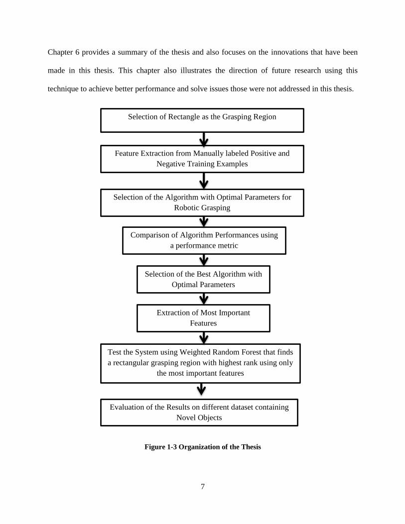
Chapter 6 provides a summary of the thesis and also focuses on the innovations that have been
made in this thesis. This chapter also illustrates the direction of future research using this
technique to achieve better performance and solve issues those were not addressed in this thesis.
Figure 1-3 Organization of the Thesis
Selection of Rectangle as the Grasping Region
Feature Extraction from Manually labeled Positive and
Negative Training Examples
Selection of the Algorithm with Optimal Parameters for
Robotic Grasping
Comparison of Algorithm Performances using
a performance metric
Selection of the Best Algorithm with
Optimal Parameters
Extraction of Most Important
Features
Evaluation of the Results on different dataset containing
Novel Objects
Test the System using Weighted Random Forest that finds
a rectangular grasping region with highest rank using only
the most important features

8
1.6 References
A. Saxena, J. Driemeyer, J. Kearns, and A.Y. Ng. 2006. Robotic grasping of novel objects:
NIPS, 2006.
Y. Jiang, S. Moseson, and A. Saxena. Efficient Grasping from RGBD Images: Learning using a
new Rectangle Representation. ICRA, pp. 3304-331, 2011.
D. Fischinger, M. Vincze, and Y. Jiang. Learning Grasps for Unknown Objects in Cluttered
Scenes. ICRA, 978-1-4673-5643, May 6-10, 2013.
I. Lenz, H. Lee, and A. Saxena. Deep Learning for Detecting Robotic Grasps. ICLR, 2013.

9
CHAPTER 2: BACKGROUND AND RELATED WORK
2.1 Introduction
Robotics Grasping has gained high attention in the field of active robotics research. A great deal
of effort has been put to develop autonomous robotic grasping algorithm. Researchers have used
various approaches to address this issue. There are a significant number of papers that have
reviewed these approaches based on the grasping mechanics and the interaction between the
object and hand [Bicchi, 2000]. Researchers have also contributed in reviewing grasping
approaches based on the hand design and control [Al-Gallaf, 1993]. This thesis will deal with the
review of grasping algorithm based on the method proposed by Sahbani et al. [Sahbani, 2011].
They have reviewed grasping algorithms from two aspects: analytical and empirical. This
chapter will also focus on grasping algorithms from these two approaches.
2.2 Chapter Objectives
Listing of grasp synthesis algorithms based on analytical approaches.
Listing of grasping algorithms based on empirical approaches.
Discussion on the grasping algorithms using both approaches
2.3 Analytical Approaches
In Sahbani et al. [Sahbani, 2011] approaches that take into account the kinematics and dynamics
in developing grasping algorithms are categorized in terms of analytical approaches. They have
addressed these approaches from two perspectives.
1. Based on the possibility of forming or finding a force closure grasp

10
2. Based on task compatibility
2.3.1 Force Closure Grasps
There have been a lot of approaches where people have developed algorithms based on the
object model. Ponce et al. proposed a method where each point in a plane face was
parameterized linearly with two parameters [Ponce, 1993]. They developed an algorithm after
forming necessary linear conditions for three and four finger force closure grasps. Liu et al. [Liu,
1999] demonstrated an algorithm where force closure grasp is achieved for n fingers. Here, n-1
fingers were fixed in a position and with these the grasp is not a force closure. They searched for
a location on the object face for the n-th finger using a linear parameterization technique where
force closure grasp will be possible. Ding et al. [Ding, 2000] proposed a method where position
of force closure grasp for all fingers was found based on an initial random grasp. These methods
have mainly considered objects as polyhedral such as boxes and selection of grasping facet is not
considered in these approaches [Sahbani, 2011].
Ding et al. [Ding, 2001] designed an approach where force closure grasps were synthesized with
7 frictionless contacts. Discretization of the grasped objects was achieved in such a way which
allowed a large number of contact wrenches to be found. In El Khoury et al. [El Khoury, 2009]
wrenches which allow the association of any three contact points that are not-aligned, forms a
basis of the wrench space. Using this result they formulated a force-closure condition which
works with general objects.
There are also lot of methods where people have tried to compare between different grasps and
tried to figure out which grasp will satisfy force-closure conditions using some criteria. Mirtich

11
et al. [Mirtich, 1994] developed one criterion to extract optimal two and three finger grasps on
2D objects. They also found optimal three finger grasps on 3D polyhedral objects. Search for an
optimal grasp in the solution space needs heavy computational effort. Because of this, some
approaches have used some predefined procedure [Fischer, 1997] or generated some random
grasps [Borst, 2003]. Some have also addressed this issue with a set of rules that were defined
prior to the grasping [Miller, 2003].
2.3.2 Task Compatibility
The prime reason of robotic grasping is to perform manipulation on different objects. Objects are
manipulated based on the type of task to be performed. Some researchers have considered
developing grasping algorithms taking into account the intended task to be performed.
Chiu et al. [Chiu, 1988] proposed an index where task compatibility is considered based on the
match of optimal direction of the manipulator and the actual direction of movement that is
required for the task to be performed. Li et al. [Li, 1988] used a measure to quantify the grasp
quality which is related to the task. Pollard et al. [Pollard, 1997] developed an algorithm that
models a task wrench space (TWS) with a unit sphere to tackle this issue. Borst et al. [Borst,
2004] came up with a method that uses object wrench space (OWS) which describes the TWS in
a specific way. To reduce the computational complexity, they modeled the OWS with a 6D
ellipsoid.
12
2.4 Empirical Approaches
Sahbani et al. [Sahbani, 2011] classified the methods which approached towards the grasping
problem using some classification and learning algorithms as empirical. These methods achieved
better computational performance over the previous analytical approaches. They further
subdivided these approaches into two sections.
1. Systems based on human observation
2. Systems based on object observation.
2.4.1 Systems based on human observation
These methods are classified as those which use some policy learning methods or learn by
demonstration where a human shows the robot how to grasp an object. The robot observes and
tries to emulate it.
In [Billard, 2008] a method describes who, what and how to emulate the operator and the robot
learns from this. In [48] a method is illustrated that considers the operator and robot are standing
in front of a table. On the table some objects are placed. The human shows the robot how to
manipulate an object. The robot then tries to emulate it. Hidden Markov model (HMM) and
magnetic trackers are used for this purpose.
In Hueser et al. [Hueser, 2006] the authors developed a method that uses vision and audio for
grasping. After demonstration of the grasping by the operator, the robot tries to track the hand of
the operator stereoscopically. In Hueser et al. [Hueser, 2008] a method was proposed using Self-
13
Organizing Maps (SOM) and Q-learning approach that follows similar approach. A vision based
approach is also presented in Romero et al. [Romero, 2008], where the system is constructed in
three parts: grasp classification, measuring the hand position relative to the object and a grasp
strategy for the robot to perform grasping.
Oztop et al. [Oztop, 2002] displayed an approach that develops a grasp strategy using the
concept of mirror neurons. Kyota et al [Kyota, 2005] proposed a method to detect grasping
positions where they found the graspable portions using a neural network. Training is done using
a data glove.
2.4.2 Systems based on object observation
Development of grasping algorithm based on this approach considers object affordances,
properties of the objects and produces an algorithm that is generalized to find a grasping location
on any object.
Pelossof et al. [Pelossof, 2004] used support vector machines in order to generate a mapping
between the shape of the object, parameters of the grasp and quality of the grasp. Stark et al.
[Stark, 2008] showed a method that uses affordance learning strategies. Li et al. [Li, 2007]
proposed a shape matching algorithm to tackle this issue. They assumed that the 3D model of the
object is available.

14
Saxena et al. [Saxena, 2006] proposed a grasping algorithm that finds a 2D point on an object
using Support Vector Machine algorithm. Saxena et al. [Saxena, 2008, 2009] used supervised
learning methods to detect a grasping point using image features on novel objects. Jiang et al.
[Jiang, 2011] proposed a rectangle region detection technique using a SVM-rank algorithm to
detect robotic grasps. Lenz et al [Lenz, 2013] used deep learning method to detect robotic grasps.
2.5 Discussion
Methods those followed the analytical approach have mainly emphasized on the concept of
finding a force-closure grasp or finding grasp based on the task. Here the most significant
problem is the computational effort, which is needed to find such a grasp from an enormously
huge search space, is very high. For task modeling the effort to model a task is also the same.
Models that have followed the empirical approaches have seen to achieve robustness in terms of
application. Human based observation methods do not completely fulfill the condition for
autonomous grasping. Developing algorithms based on object observation have gained much
popularity among researchers due to its high performance. Pre-modelling an object is always
difficult. So, the methods that consider in learning from features using some supervised learning
algorithm is better implemented in practice and also acts as a motivation for this work.
2.6 References
A. Bicchi, V. Kumar. Robotics Grasping and Contact: A review. ICRA 2000.

15
E. Al-Gallaf, A. Allen, K. Warwick. A survey of Multi-fingered Robotic Hands: Issues and
grasping achievements. 1993, Mechatronics 01/1993; DOI: 10. 1016/0957-4158(93)
90018-W
A. Saxena, J. Driemeyer, J. Kearns, and A.Y. Ng. 2006. Robotic grasping of novel objects:
NIPS, 2006.
Y. Jiang, S. Moseson, and A. Saxena. Efficient Grasping from RGBD Images: Learning using a
new Rectangle Representation. ICRA, pp. 3304-331, 2011.
I. Lenz, H. Lee, and A. Saxena. Deep Learning for Detecting Robotic Grasps. ICLR, 2013.
A. Sahbani, S. El-Khoury, P. Bidaud, An overview of 3D grasp synthesis algorithms, Robotics
and Autonomous Systems, 2011, doi:10.1016/j.robot. 2011
J. Ponce, S. Sullivan, J. D. Boissonnat, J. P. Merlet. On characterizing and computing three and
four finger force closure grasps of polyhedral objects. IEEE International Conference on
Robotics and Automation, vol. 2, 1993, pp. 821-827.
Y. H. Liu. Qualitative test and force optimization of 3-D frictional form closure grasps using
linear programming. IEEE Transactions on Robotics and Automation 15 (1), 1999.

16
D. Ding, Y. H. Liu, S. Wang. Computing 3D optimal form closure grasps. IEEE International
Conference on Robotics and Automation, vol4. 2000, pp. 3573-3578.
D. Ding, Y. H. Liu, S. Wang. On computing immobilizing grasps of 3-D curved objects. IEEE
International Symposium on Computational Intelligence in Robotics and Automation,
2001, pp. 11-16.
S. El-Khoury, A. Sahbani. On computing robust N-finger force closure grasps of 3D objects,
ICRA 2009, pp. 2480-2486.
B. Mirtich, J. Canny. Easily computable optimum grasps in 2D and 3D, ICRA 1994, vol 1, pp.
739-747.
C. Borst, M. Fischer, G. Hirzinger. Grasping the dice by dicing the grasp. ICRA 2003, vol 3, pp
3692-3697.
M. Fischer, G. Hirzinger. Fast planning of precision grasps for 3D objects. ICRA 1997, pp. 120-
126.

17
A. T. Miller, P. K. Allen. Examples of 3D grasp quality computations. ICRA 1999, pp. 1240-
1246.
S. Chiu. Task Compatibility of manipulator postures, International Journal of Robotics Research
7 (5), 1988, 13-21.
Z. Li, S.S. Sastry. Task Oriented optimal grasping by multi-fingered robot hands. International
Journal of Robotics and Automation 4 (1), 1988.
N. S. Pollard, Parallel algorithms for synthesis of whole hand grasps, IEEE International
Conference on Robotics and Automation, vol. 1, 1997, pp. 373-378.
A. Billard, S. Calinon, R. Dillmann, S. Schaal, Survey: Robot Programming by demonstration.
Handbook of Robotics, MIT Press, 2008.
S, Ekvall, D. Kragic, Interactive grasp learning based on human demonstration. ICRA, 2004,
vol. 4, pp. 3519-3524.

18
F. Kyota, T. Watabe, S. Saito, M. Nakajima, Detection and evaluation of grasping positions for
autonomous agents. International Conference on Cyberworlds, 2005, pp. 453-460.
M. Hueser, T. Baier, J. Zhang. Learning of demonstrated grasping skills by steresocoping
tracking of human hand configuration. ICRA 2006, pp. 2795-2800.
J. Romero, H. Kjellstrom, D. Kragic, Human-to-robot mapping of grasps. ICRA, WS on Grasp
and Task Learning by imitation, 2008, 9-15.
E. Oztop, M. A. Arbib. Schema design and implementation of the grasp related mirror neuron
system, Biological Cybernatics 87 (2), 2002, 116-140.
M. Hueser, J. Zhang. Visual and Contact-free imitation learning of demonstrated grasping skills
with adaptive environment modelling. IEEE/RSJ International Conference on Intelligent
Robots and Systems, WS on Grasp and Task Learning by Imitation, 2008, pp. 17-24.
R. Pelossof, A. Miller, P. Allen, T. Jebara. An SVM Learning approach to robotic grasping.
ICRA 2004, vol. 4, pp. 3512-3518.

19
Y. Li, J. L. Fu, N. Pollard. Data driven grasp synthesis using shape matching and task based
pruning. IEEE Transactions on Visualization and Computer Grasphics. 13 (4), 2007, 732-
747.
M. Stark, P. Lies, M. Zillich, B. Schiele. Functional object class detection based on learned
affordance cues. International Conference on Computer Vision Systems, 2008, pp. 435-
444.
A. Saxena, J. Driemeyer and A. Ng. Robotic Grasping of Novel Objects using Vision. IJRR, vol.
27, no.2, Multimedia Archives, 2008, p. 157.
A. Saxena, Monocular Depth perception and robotic grasping of novel objects. PhD Dissertation,
Stanford University, 2009.

20
CHAPTER 3: FEATURES USED AND EXTRACTION TECHNIQUE
3.1 Introduction
3.1.1 Feature Extraction
Both image and point cloud features are used in this method. Features are extracted from a set of
labeled rectangles. Those labels are manually assigned on an object that corresponds to good and
bad grasps. Rectangles with good grasping regions are denoted as Positive examples and others
as negative examples. This method exploits a high number of features for extraction from the
positive and negative rectangles. For the grasping system the features those have higher
information content are mainly used. Feature extraction is performed before the Training step of
the algorithm.
Figure 3-1: Features are extracted from subdividing the rectangle into Top, Middle and Bottom
Horizontal strips.
In order to capture more details of an object, each rectangle is subdivided into three horizontal
strips. Features are then extracted from each strip using a 15 binned histogram. It is seen that
extraction of features in this method performs better than extracting features from the whole
rectangle at a time. The feature extraction technique in this method is followed from Lim et al.
Middle
Top
Bottom
FT
FM
FB

21
[Lim 2010], Saxena et al. [Saxena, 2008] and Jiang et al.[Jiang 2011]. The concept of using
binned histograms, Image and Point cloud Feature is used from Lim et al. [Lim 2010]. The
feature extraction technique using color, edge and texture cues and the extraction technique of
using 9 Laws’ mask to extract texture features, 6 Oriented edge filters to extract edge
information and First Laws’ mask to extract color information are followed from Saxena et al
[Saxena, 2008]. The concept of using Non-linear features that uses the ratio of the top, bottom
and middle section of the rectangle are followed from Jiang et al [Jiang, 2011]. Those features
and extraction technique are discussed in detail here for convenience.
This method uses a total 2110 features in the implementation of the system. Among them 1530
are Image Features, 270 Point Cloud Features, 308 Viewpoint Feature Histogram Descriptor
(VFH) based features and 2 geometric features. This chapter deals with the description of these
features and the extraction technique that is employed for feature collection from labeled
rectangles.
Figure 3-2 Total Number of Features in this Method
3.2 Chapter Objectives
Description of Image Feature and Extraction Technique.
Description of Point Cloud Feature and Extraction Technique.
Description of Viewpoint Feature Histogram Descriptors and Feature Extraction
Technique.
Image Features+ Point Cloud Features+ VFH Features + Height + Width
1530+270+308+1+1
2110
22
Description of the Geometric Features used.
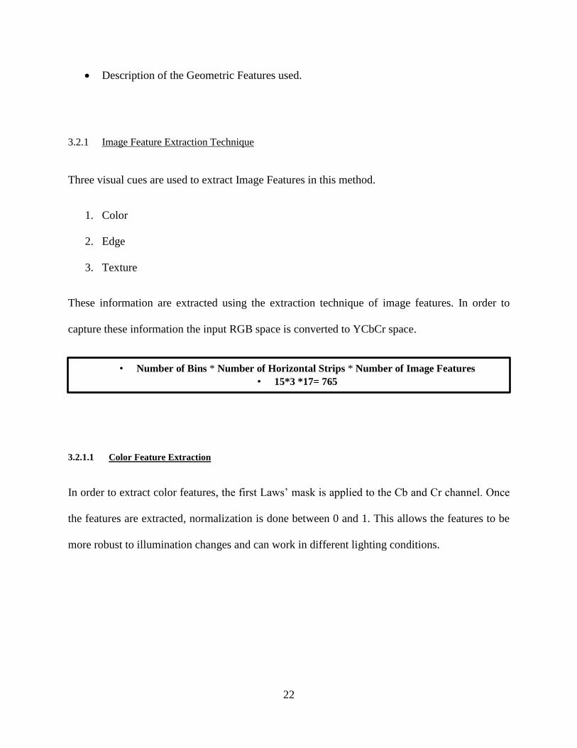
3.2.1 Image Feature Extraction Technique
Three visual cues are used to extract Image Features in this method.
1. Color
2. Edge
3. Texture
These information are extracted using the extraction technique of image features. In order to
capture these information the input RGB space is converted to YCbCr space.
3.2.1.1 Color Feature Extraction
In order to extract color features, the first Laws’ mask is applied to the Cb and Cr channel. Once
the features are extracted, normalization is done between 0 and 1. This allows the features to be
more robust to illumination changes and can work in different lighting conditions.
• Number of Bins * Number of Horizontal Strips * Number of Image Features
• 15*3 *17= 765

23
Figure 3-3: Image Feature Extraction Technique
From each strip there will be 15 x 2=30 color features. So, from each rectangle there will be 30 x
3=90 color features. Histogram of Color Features extracted from Positive and Negative
Rectangles are displayed in Figure 3-4.
Cb
R G B
Y Cr
Local Averaging Filter
Normalization
Output
Input
Number of Bins * Number of Horizontal Strips * Number of Color Features
15 *3 *2 =90
24
Figure 3-4 Color Features Extracted from (left) Positive Rectangles (right) Negative Rectangles
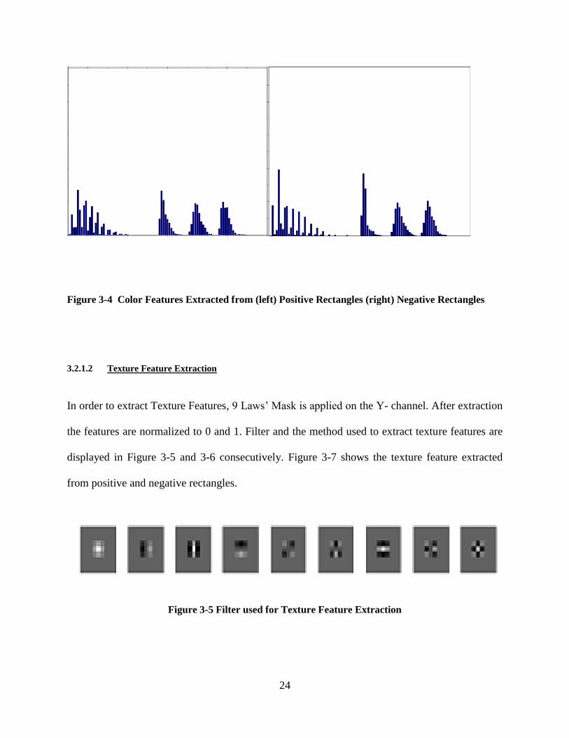
3.2.1.2 Texture Feature Extraction
In order to extract Texture Features, 9 Laws’ Mask is applied on the Y- channel. After extraction
the features are normalized to 0 and 1. Filter and the method used to extract texture features are
displayed in Figure 3-5 and 3-6 consecutively. Figure 3-7 shows the texture feature extracted
from positive and negative rectangles.
Figure 3-5 Filter used for Texture Feature Extraction
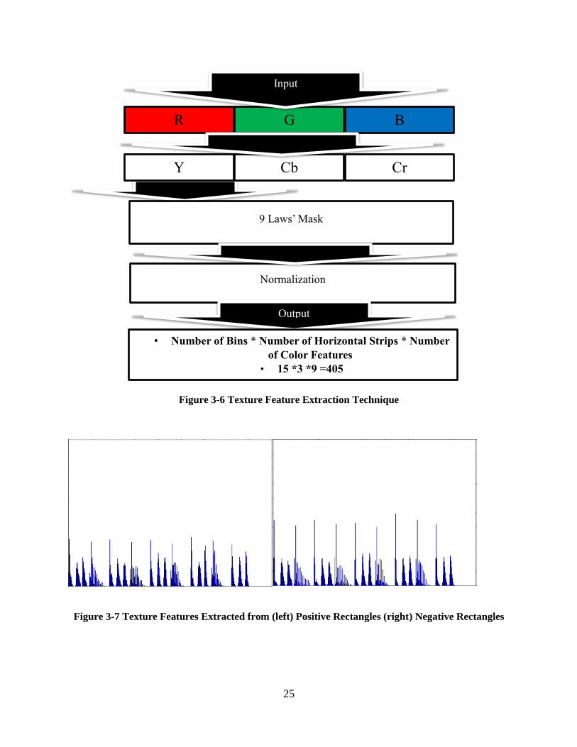
25
Figure 3-6 Texture Feature Extraction Technique
Figure 3-7 Texture Features Extracted from (left) Positive Rectangles (right) Negative Rectangles
Cb
R G B
Y Cr
9 Laws’ Mask
Normalization
Output
Input
• Number of Bins * Number of Horizontal Strips * Number
of Color Features
• 15 *3 *9 =405

26
3.2.1.3 Edge Feature Extraction
Edge Features are extracted by convolving the Y-channel with 6 oriented edge filters. After
extraction of the features the values are normalized to 0 and 1. Edge Filters used in this system
and the technique employed to extract edge features are displayed in Figure 3-8 and 3-9.
Figure 3-8 Filters used to extract Edge Features
Figure 3-9 Edge Feature Extraction Technique
Cb
R G B
Y Cr
6 Oriented Edge Filters
Normalization
Output
Input
• Number of Bins * Number of Horizontal Strips * Number of
Color Features
• 15*3 *6 =270

27
From each strip there will be 15 x 6 =90 edge features. So, from each rectangle there will be 90 x
3=270 features. Histogram of Edge features extracted from Positive and Negative examples are
displayed in Figure 3-10.
Figure 3-10 Texture Feature Extracted from (left) Positive and (right) Negative Examples
3.2.2 Non-linear Image Feature Extraction Technique
For extraction of non-linear image feature, ratios of the feature values between top, middle and
bottom strips are used. These are also used as the advanced features.
3.2.2.1 Non-linear Color Feature Extraction
Ratios of the color features from three strips of a rectangle are used. The features used are
𝐹𝑇𝑐/𝐹𝑀𝑐
, 𝐹𝐵𝑐/𝐹𝑀𝑐
, (𝐹𝑇𝑐. 𝐹𝐵𝑐
)/𝐹𝑀𝑐. Here, from each strip there will be 30 features. So, from each
rectangle there will be 90 features. Non-linear color features extracted from positive and negative
rectangles are shown in this Figure 3-11.
• Number of Bins * Number of Horizontal Strips * Number of Non Linear Image
Features
• 15*3 *17= 765
28
Figure 3-11Nonlinear Color Features Extracted from (left) Positive Rectangles (right) Negative
Rectangles
3.2.2.2 Non-linear Texture Feature Extraction
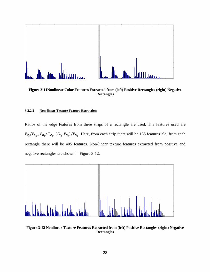
Ratios of the edge features from three strips of a rectangle are used. The features used are
𝐹𝑇𝑡/𝐹𝑀𝑡
, 𝐹𝐵𝑡/𝐹𝑀𝑡
, (𝐹𝑇𝑡. 𝐹𝐵𝑡
)/𝐹𝑀𝑡. Here, from each strip there will be 135 features. So, from each
rectangle there will be 405 features. Non-linear texture features extracted from positive and
negative rectangles are shown in Figure 3-12.
Figure 3-12 Nonlinear Texture Features Extracted from (left) Positive Rectangles (right) Negative
Rectangles

29
3.2.2.3 Non-linear Edge Feature Extraction
Ratios of the edge features from three strips of a rectangle are used. The features used are
𝐹𝑇𝑒/𝐹𝑀𝑒
, 𝐹𝐵𝑒/𝐹𝑀𝑒
, (𝐹𝑇𝑒. 𝐹𝐵𝑒
)/𝐹𝑀𝑒. Here, from each strip there will be 90 features. So, from each
rectangle, there will be 270 features. Non-linear edge features extracted from positive and
negative rectangles are shown in Figure 3-13.
Figure 3-13 Nonlinear Edge Features Extracted from (left) Positive Rectangles (right) Negative
Rectangles
3.2.3 Point Cloud Feature Extraction Technique
Three cues are used for extraction of point cloud features. In total 270 point cloud
features are extracted. Cues used are
1. Depth
2. Surface Normal
3. Surface Curvature
• Number of Bins * Number of Horizontal Strips * Number of Point Cloud Features
• 15*3 *3= 135

30
3.2.3.1 Depth Feature Extraction
Figure 3-14 Depth Feature Extraction from (left) Positive Rectangles (right) Negative Rectangles
Z-positional value is used as the depth feature in this method from the point cloud collected.
This corresponds to the viewpoint component so we do not consider X and Y information.
Histogram of depth features extracted from positive and negative examples are illustrated below.
For each strip there will be 15 features. So, from a rectangle there will be 15 x 3= 45 depth
features.
3.2.3.2 Surface Normal Feature Extraction
In order to extract surface normal features a surface is fitted though the point and its 50
neighboring points. From each strip there will be 15 surface normal features. So, from a
rectangle 15 x 3= 45 features are extracted. Histogram of surface normal extracted from the
positive and negative rectangle is shown in Figure 3-15.

31
Figure 3-15 Surface Normal Features Extracted from (left) Positive Rectangles (right) Negative
Rectangles
3.2.3.3 Surface Curvature Feature Extraction
Surface curvature feature extraction technique is also similar to normal feature extraction. Here
also, a surface is fitted through the point and its 50 neighboring points and surface curvatures are
computed. Each strip outputs 15 features. So, one rectangle produces 15 x 3= 45 surface
curvature features. Histogram of surface curvature features extracted from positive and negative
rectangles are shown in Figure 3-16.
Figure 3-16 Surface Curvature Features Extracted from (left) Positive Rectangles (right) Negative
Rectangles
y = 1106.4x - 291.88 R² = 0.9376
0
500
1000
1500
2000
0 1 2
1/q
(g
me
dia∙m
g-1-P
)
1/Ce
y = 1106.4x - 291.88 R² = 0.9376
0
500
1000
1500
2000
0 1 2
1/q
(g
me
dia∙m
g-1-P
)
1/Ce
y = 1106.4x - 291.88 R² = 0.9376
0
500
1000
1500
2000
0 1 2
1/q
(g
me
dia∙m
g-1-P
)
1/Ce
y = 1106.4x - 291.88 R² = 0.9376
0
500
1000
1500
2000
0 1 2
1/q
(g
me
dia∙m
g-1-P
)
1/Ce

32
3.2.4 Non-linear Point Cloud Feature Extraction Technique
For Non-linear Point cloud feature extraction, ratios of the features values from top, middle and
bottom strips are used. There will be 135 more features extracted in this technique.
3.2.4.1 Non-linear Depth Feature Extraction
Ratios of the depth from three strips constitute this feature. Values of 𝐹𝑇𝐷
𝐹𝑀𝐷
,𝐹𝐵𝐷
𝐹𝑀𝐷
, 𝐹𝑇𝐷.𝐹𝐵𝐷
𝐹𝑀𝐷
are used
as the features. There will be 45 non-linear features from each rectangle with 15 from each strip.
Histogram of features from positive and negative examples is shown in Figure 3-17.
Figure 3-17 Non-linear Depth Features Extracted from (left) Positive Rectangles (right) Negative
Rectangles
y = 1106.4x - 291.88 R² = 0.9376
0
500
1000
1500
2000
0 1 2
1/q
(g
me
dia∙m
g-1-P
)
1/Ce
y = 1106.4x - 291.88 R² = 0.9376
0
500
1000
1500
2000
0 1 2
1/q
(g
me
dia∙m
g-1-P
)
1/Ce
• Number of Bins * Number of Horizontal Strips * Number of Non-linear Point Cloud
Features
• 15*3 *3= 135

33
3.2.4.2 Non-linear Surface Normal Feature Extraction
Ratios of the surface normal from three strips constitute this feature. Values of
𝐹𝑇𝑁
𝐹𝑀𝑁
,𝐹𝐵𝑁
𝐹𝑀𝑁
, 𝐹𝑇𝑁.𝐹𝐵𝑁
𝐹𝑀𝑁
are used as the features. There will be 45 non-linear features from each
rectangle with 15 from each strip. Histogram of features from positive and negative examples is
shown in Figure 3-18.
Figure 3-18 Non-linear Surface Normal Features Extracted from (left) Positive Rectangles (right)
Negative Rectangles
3.2.4.3 Non-linear Surface Curvature Feature Extraction
Ratios of the surface curvature features from three strips constitute this feature. Values of
𝐹𝑇𝑠𝑐
𝐹𝑀𝑠𝑐
,𝐹𝐵𝑠𝑐
𝐹𝑀𝑠𝑐
, 𝐹𝑇𝑠𝑐.𝐹𝐵𝑠𝑐
𝐹𝑀𝑠𝑐
are used as the features. There will be 45 non-linear features from each
rectangle with 15 from each strip. Histogram of features from positive and negative examples is
shown in Figure 3-19.
y = 1106.4x - 291.88 R² = 0.9376
0
500
1000
1500
2000
0 1 2
1/q
(g
me
dia∙m
g-1-P
)
1/Ce
y = 1106.4x - 291.88 R² = 0.9376
0
500
1000
1500
2000
0 1 2
1/q
(g
me
dia∙m
g-1-P
)
1/Ce

34
Figure 3-19 Non-linear Surface Normal Features Extracted from (left) Positive Rectangles (right)
Negative Rectangles
3.2.5 Fast Point Feature Histogram Descriptors Extraction Technique
Viewpoint Feature Histogram descriptor is a significant feature that captures the geometrical
properties of a point and its’ neighborhood. The viewpoint Feature Histogram (VFH) descriptor
is similar to Fast Point Feature Histogram descriptor [Rusu, 2009]. Because of its speed and
discriminative power, VFH feature is used in this method. VFH feature has been very
successfully implemented in the field of object detection and pose estimation problem. The key
idea in VFH feature is to use the discriminative feature of FPFH descriptors with respect to a
viewpoint direction. The VFH Feature concept is introduced and used in practice by Rusu et al.
[Rusu, 2010].
To compute the VFH features, the concept of mixing the viewpoint direction directly into the
relative normal angle calculation is employed. FPFH features are described in detail in Appendix
B. The viewpoint component is calculated by using a histogram of angles which is produced
y = 244.67x + 196.37 R² = 0.8594
0
200
400
600
800
1000
1200
1400
0 1 2 3 4
1/q
(g
me
dia∙m
g-1-P
)
1/Ce (L∙mg-1)
y = 244.67x + 196.37 R² = 0.8594
0
200
400
600
800
1000
1200
1400
0 1 2 3 4
1/q
(g
me
dia∙m
g-1-P
)
1/Ce (L∙mg-1)

35
between the view-point with each normal. In order to ensure the scale invariance the angle
between the central viewpoint directions is translated to each normal.
The computation of second component of VFH feature is quite similar to FPFH feature
computation. But here, instead of using each normal, the relative pan, tilt and yaw angles are
measured using the viewpoint direction at the central point and each normal on the surface. The
Euclidean distance between the centroid from each point constitutes the other part of the second
component. This is also known as surface shape component.
This method exploits the usage of 45 binning histograms for each of the three angle component
of the FPFH. Additional 45 binning histograms are used which measures the Euclidean distance
between the centroid and each point on the surface. This makes the VFH feature number, 180.
128 more binning histograms are used for the viewpoint component. In total, 308 VFH features
are used in this system.
Figure 3-20 Viewpoint Feature Histogram Descriptors from (left) Positive Examples (right)
Negative Examples

36
3.2.6 Geometric Feature Extraction Technique
In order to capture geometric information of an object, height and width are used as geometric
features. These two features also provide some distinctive information between good and bad
grasping rectangles.
3.3 Discussion
This chapter demonstrates the features, those are used in the system to train the robot so that it
can learn in distinguishing between Positive and Negative grasps. A total of 2110 Image and
Point Cloud Features are used. Histograms collected for each feature on some from the
rectangles (both positive and negative) depict that these feature are capable to provide the
discrimination between good and bad grasps. To my knowledge, VFH feature is used in the area
of autonomous grasping for the first time in this method. This feature aids in achieving
significant accuracy over FPFH features used in some other methods.
3.4 References:
Y. Jiang, S. Moseson, and A. Saxena. Efficient Grasping from RGBD Images: Learning using a
new Rectangle Representation. ICRA, pp. 3304-331, 2011.
A. Saxena, J. Driemeyer and A. Ng. Robotic Grasping of Novel Objects using Vision. IJRR, vol.
27, no.2, Multimedia Archives, 2008, p. 157.

37
R. Rusu et al. Fast Point Feature Histograms (FPFH) for 3D Registration, ICRA. 2009.
R. B. Rusu, G. Bradski, R. Thibaux, J. Hsu. Fast 3D Recognition and Pose Using the Viewpoint
Feature Histogram, Proceedings of the 23rd
IEEE/RSJ International Conference on
Intelligent Robots and Systems (IROS), 2010.
M. Lim, B. Biswal. Determining Grasping Region Using Vision. Cornell University.

38
CHAPTER 4: WHY RANDOM FOREST?
4.1 Introduction
The selection of machine learning algorithm is a challenging problem in the research community.
For autonomous grasping of unknown objects, usage of a supervised learning algorithm has been
very successful. Supervised learning algorithm enables the robot to learn from the labeled data.
In this method, to learn from the labeled rectangles weighted random forest algorithm is used.
Selection of the weighted random forest algorithm is not performed at random here. It was
chosen over other commonly available and very successful supervised learning algorithms, using
some performance metric results.
The performance metric used in this method to compare between Support Vector Machine,
Decision Tree, Adaboost and Weighted Random Forest Algorithm utilizes the error estimates
which are used to analyze a system performance and the execution time. For autonomous robotic
grasping to be applicable in assistive robotics the most important issue to be satisfied is the
ability of the algorithm to achieve highest possible success rate in minimum possible time,
literally real time. The performance metric ensures the selection of the best algorithm can lead
towards the best performance.
Efficient usage of machine learning algorithm does not only depend on selection of the best
algorithm. The parameters associated with an algorithm are also tremendously vital. Poor
selection of parameters will totally disrupt the performance of the system. In addition for

39
selection of the proper algorithm for a given dataset, a performance metric algorithm can be
utilized in selecting the optimal parameters associated with the algorithm. In this method this
technique is employed in selecting the best algorithm with optimal parameters. The chosen
algorithm with the selected optimal parameters will perform the best for a dataset.
In this method the performance metric compares the performance between Support Vector
Machine with Linear, Polynomial and Radial Basis Function Kernel, Decision Tree, Adaboost
and Random Forest Algorithm with different number of trees and other associated parameters
which influence the algorithm performance. The performance metric uses Cross Validation
Score, Accuracy, Precision, Receiver Operating Characteristics (ROC) score, F1 score and recall
as the error estimates and the running time of an algorithm as execution time parameter. The
error estimates used in this method are defined below. For Training Cornell University Personal
Robotics dataset is used. 66.66% of the data (5000 examples from 7037) were used for training
and rest for testing.
4.1.1 Cross Validation Score
Cross-validation score is a measure to assess how the statistical analysis will be generalized in an
independent dataset. It determines how accurately a predictive model will perform. It is used for
comparison of the performance of two or more different algorithms and selecting the best
algorithm for the available data, or alternatively to compare the performance of two or more
variance of a parameterized model.

40
4.1.2 Precision
Precision is the fraction of the examples retrieved which have relevance to the find. It takes into
account all the retrieved examples but can be evaluated only at a given cut-off rank which
considers only the topmost results returned by the system. This is called as precision at n. It is
defined as,
𝑃𝑟𝑒𝑐𝑖𝑠𝑖𝑜𝑛 =𝑇𝑃
𝑇𝑃 + 𝐹𝑃… … (4.1)
4.1.3 Recall
In the field of machine learning, Recall is defined as the portion or fraction of the examples that
have relevance to the query which are successfully retrieved. In binary classification problem, it
is also known as sensitivity. It can also be regarded as the probability by which a relevant
example is retrieved by any query. The equation to compute recall is,
𝑅𝑒𝑐𝑎𝑙𝑙 =𝑇𝑃
𝑇𝑃 + 𝐹𝑁… … (4.2)
4.1.4 Accuracy
This is associated with trueness of systemic errors and precision with random errors.
Accuracy is defined as a combination of both trueness and precision. This is ratio of the true
examples in the entire population. It is also sometimes referred as “Rand Accuracy”. It is called a
parameter of the test. The method for computing accuracy is,

41
𝐴𝑐𝑐𝑢𝑟𝑎𝑐𝑦 =𝑇𝑃 + 𝑇𝑁
𝑇𝑃 + 𝐹𝑃 + 𝐹𝑁 + 𝑇𝑁… … (4.3)
4.1.5 F1 Score
F1 score is a measure of test’s accuracy. In computation of the score it takes into account both
the precision and recall. It can be described as a weighted average of precision and recall also. It
does not take into account the true negative rate. It can be defined as,
𝐹1 = 2.𝑝𝑟𝑒𝑐𝑖𝑠𝑖𝑜𝑛 × 𝑟𝑒𝑐𝑎𝑙𝑙
𝑝𝑟𝑒𝑐𝑖𝑠𝑖𝑜𝑛 + 𝑟𝑒𝑐𝑎𝑙𝑙… … (4.4)
It is actually the harmonic mean of precision and sensitivity. It can be simplified as,
𝐹1 =2𝑇𝑃
(2𝑇𝑃 + 𝐹𝑃 + 𝐹𝑁)… … (4.5)
4.1.6 ROC Score
ROC score determines the area under the ROC curve. ROC Curve illustrates the performance of
a classifier when the discrimination threshold is varied accordingly. The ROC curve displays the
true positive rate vs false positive rate variation. False Positive Rate is also known as fall-out. So,
it is actually a measure of the sensitivity as a function of fall-out.
All these error estimates are extracted out from each algorithm and upon comparison with
execution time, performance metric is evaluated which is discussed in detail in this chapter.
42
4.2 Chapter Objectives
Definition of Performance Metric.
Comparison of the performance metric results on support vector machine with different
kernel.
Comparison of the performance metric results on Decision Tree algorithm with different
parameters.
Comparison of the Adaboost Algorithm with various important parameters.
Selection of the range of number of Trees for Random Forest Algorithm.
Comparison of the Weighted Random Forest Algorithm with different trees and varying
parameters.
Selection of the Best learning Algorithm.
Selection of the most significant features that allows reducing search space maintaining
the accuracy.
4.3 Definition of Performance Metric
Classification is one of the most exciting areas in the field of machine learning research. From
vast of classification algorithms it has always been a basic science question “Which algorithm
should be the first choice for my classification task”? People have adopted different techniques
in doing so. In this thesis, a method similar to Ali et al. [Ali, 2004] is used in order to select the
classification algorithm. They have defined a performance metric, Z as a linear function of error
estimates and execution time. The definition of performance metric, Z is shown in Equation 4.6.
𝑍 = 𝛼𝑒𝑖 + 𝛽𝑐𝑖 … … (4.6)
Here,
Z= Performance Metric
𝑒= Error estimates (accuracy, cross-validation score, F-1 score, precision, recall, ROC )
𝑐= Execution time
𝛼=average accuracy weight

43
𝛽=Weight for computation time
Ali et al. [Ali, 2004] used the value of 𝜶 to be constant and set it to 1. They varied the value of 𝜷
from 0 to 2 in order to find the performance metric, Z and the algorithm that has the highest Z
value is considered to perform the best. They used True Positive Rate (TPR), True Negative Rate
(TNR), F1 Score and Accuracy as the error estimates.
The method proposed in this thesis, uses the same definition of performance metric in order to
find the best classifier with optimal criterions but uses a slight different technique in choice of
error estimates and fixing the value of 𝜷. In this method, accuracy, precision, recall, ROC Score,
F1 score, Cross Validation Score are used as error estimates and an average of them is used as 𝑒𝑖.
The value of 𝛼 is kept at 1. 𝜷 is varied from 1 to 11 here and the value of the performance
metric Z is measured for different algorithms and compared further.
4.4 Support Vector Machine
Support Vector Machine Algorithm is one of the most commonly used machine learning
algorithm in robotic grasping. It is a supervised learning method that analyzes data and figures
out patterns when used for classification. It is also vastly used for regression analysis
applications. It is a representation of the examples as points in the space. This performs a
mapping such a way that the examples of different categories are separated by a large margin or
gap. This margin is expected to be as wide as possible. When new examples are mapped onto the
same space then the predictive model of SVM determines on which side of the gap that example
belongs. Using Kernel trick, SVM can be used for both linear and non-linear classification. In

44
non-linear classification SVM implicitly models the examples in a higher dimensional space by
employing similar mapping techniques.
Support Vector Machine can be described as an algorithm that forms a hyper-plane or set of
hyper-planes in a high dimensional space. The hyper-plane that provides the largest margin to
the nearest training data examples are known to perform better and lowers the generalization
error. When mapping is done in higher dimensional space in order to keep the computational
complexity simpler, it is mapped such a way that the dot products are easily computed by using
some kernel function, k (x, y). The hyper-planes are defined in a way so that they ensure their
dot products with any vector in that specific space remains constant. SVM algorithm is first
proposed by Vapnik et al. [Vapnik, 1995].
In the later sections, SVM with both Linear and Non-linear kernels are discussed. Degree 3
Polynomial kernel and Radial Basis Function Kernel are used as Non-linear kernels for SVM in
this method. SVM was implemented using scikit-learn in python. [Pedregosa, 2011].
4.4.1 SVM with Linear kernel
In case of a SVM with linear kernel, a data point is described as n-dimensional vector and the
goal is determining whether those points are separated by n-1 dimensional hyper-plane. There
may be more than one hyper-plane that can classify the data points. But, the one that has the
largest separation is chosen as the best hyper-plane between two classes. That is why, the hyper-

45
plane that has the maximum distance from its nearest data point is chosen. If such a hyper-plane
can be found for a problem setting that is known as the maximum-margin hyper-plane.
4.4.2 Parameters used in SVM with linear kernel and Results
The set of Parameters used in the SVM with Linear Kernel is illustrated below
Figure 4-1Confusion Matrix and ROC Curve of Linear SVM
The error estimates like ROC curve and Confusion Matrix obtained from linear Kernel are
displayed in Figure 4-1.
Parameters in Linear SVM
1. C=1
2. Class Weight= None.
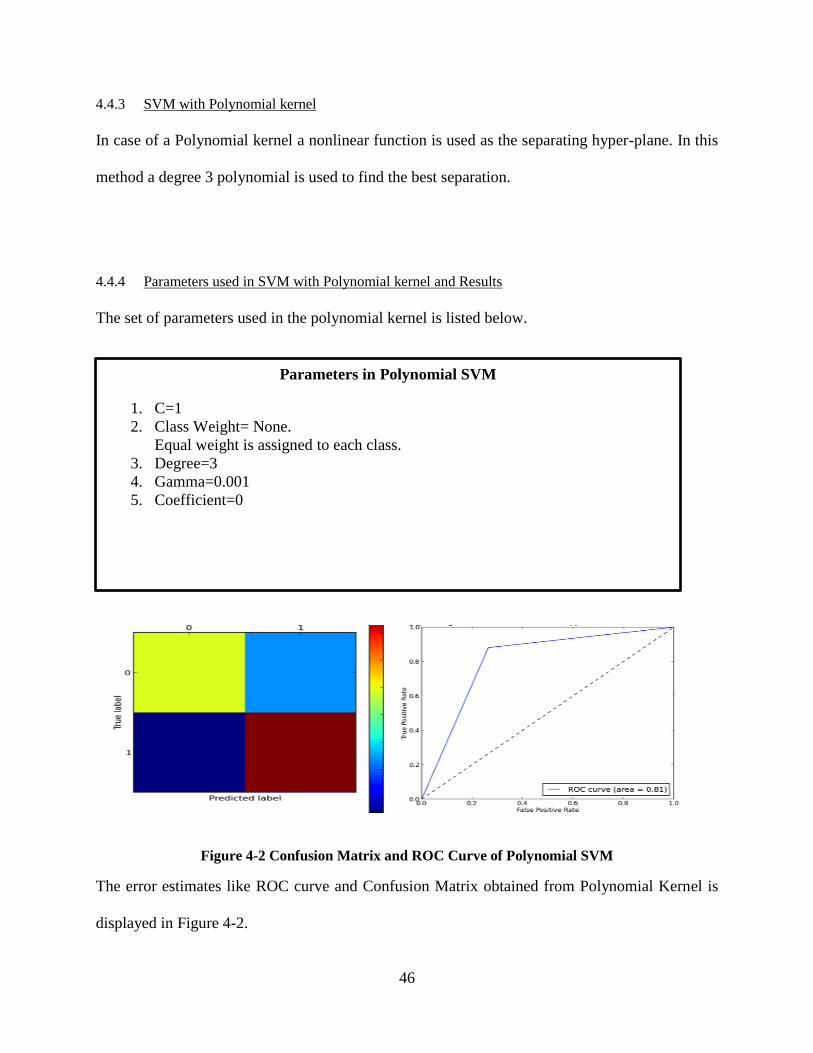
46
4.4.3 SVM with Polynomial kernel
In case of a Polynomial kernel a nonlinear function is used as the separating hyper-plane. In this
method a degree 3 polynomial is used to find the best separation.
4.4.4 Parameters used in SVM with Polynomial kernel and Results
The set of parameters used in the polynomial kernel is listed below.
Figure 4-2 Confusion Matrix and ROC Curve of Polynomial SVM
The error estimates like ROC curve and Confusion Matrix obtained from Polynomial Kernel is
displayed in Figure 4-2.
Parameters in Polynomial SVM
1. C=1
2. Class Weight= None.
Equal weight is assigned to each class.
3. Degree=3
4. Gamma=0.001
5. Coefficient=0

47
4.4.5 SVM with Radial Basis Function kernel
It is also a popular kernel function in machine learning algorithms. In this method a very low
gamma value is used and no weight is assigned to any of the classes.
4.4.6 Parameters used in SVM with Radial Basis Function kernel and Results
The set of Parameters used in the SVM with Radial Basis Function Kernel is illustrated below.
Figure 4-3 Confusion Matrix and ROC Curve of RBF SVM
The Error estimates like ROC curve and Confusion Matrix obtained from Polynomial Kernel is
displayed in Figure 4-3.
Parameters in Radial Basis Function SVM
1. C=1
2. Class Weight= None.
Equal weight is assigned to each class.
3. Degree=3
4. Gamma=0.001
5. Coefficient=0

48
4.4.7 Comparison of Error Estimates from Linear, Polynomial and RBF SVM and Discussion
Error Estimate Results obtained from Linear, Polynomial and RBF SVM are tabulated in Table
4-1. The table demonstrates that Linear SVM has better performance than other kernels in terms
of cross validation score, accuracy, F1 score, Precision and ROC Score. Polynomial kernel has
the best recall value than others. In this thesis a 5-fold cross validation is used.
Table 4-1Comparison of Error Estimates from Linear, Polynomial and RBF SVM
Kernel Cross
Validation
Score
Accuracy F1 Score Precision Recall ROC
Score
Linear .899
.910 .912 .931 .894 .910
Polynomia
l
.803
.817 .845 .763 .946 .809
Radial
Basis
Function
.804 .812 .831 .788 .880 .808
4.4.8 Evaluation Metric Results from Linear, Polynomial and RBF SVM
Evaluation metric results from Linear, Polynomial and RBF SVM are displayed in Figure 4-4.
From the Figure it is obvious that Linear SVM achieves the highest Z value as 𝜷 is varied. So,
linear kernel should be chosen over Polynomial and RBF kernel for classification.

49
Figure 4-4 Evaluation Metric Results for Linear, Polynomial and RBF SVM
4.5 Information Gain Parameter Definition for Tree based Learning Algorithms
For tree based learning method information gain parameters play a very important role. Those
parameters are defined here.
4.5.1 Gini Impurity
It measures the correctness of a randomly selected element if it was randomly labeled based on
the label distribution in a dataset. It can be calculated by summing the product of the probability
of how many times each item is chosen and the probability of a mistake in classification.
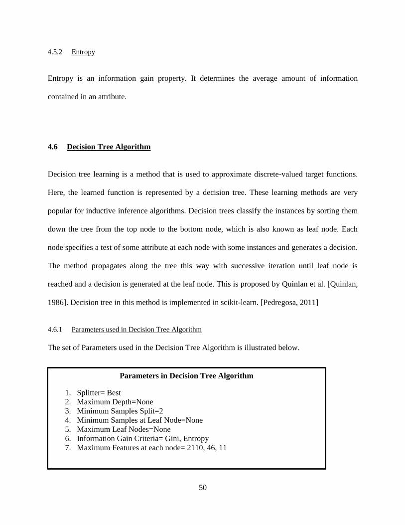
50
4.5.2 Entropy
Entropy is an information gain property. It determines the average amount of information
contained in an attribute.
4.6 Decision Tree Algorithm
Decision tree learning is a method that is used to approximate discrete-valued target functions.
Here, the learned function is represented by a decision tree. These learning methods are very
popular for inductive inference algorithms. Decision trees classify the instances by sorting them
down the tree from the top node to the bottom node, which is also known as leaf node. Each
node specifies a test of some attribute at each node with some instances and generates a decision.
The method propagates along the tree this way with successive iteration until leaf node is
reached and a decision is generated at the leaf node. This is proposed by Quinlan et al. [Quinlan,
1986]. Decision tree in this method is implemented in scikit-learn. [Pedregosa, 2011]
4.6.1 Parameters used in Decision Tree Algorithm
The set of Parameters used in the Decision Tree Algorithm is illustrated below.
Parameters in Decision Tree Algorithm
1. Splitter= Best
2. Maximum Depth=None
3. Minimum Samples Split=2
4. Minimum Samples at Leaf Node=None
5. Maximum Leaf Nodes=None
6. Information Gain Criteria= Gini, Entropy
7. Maximum Features at each node= 2110, 46, 11
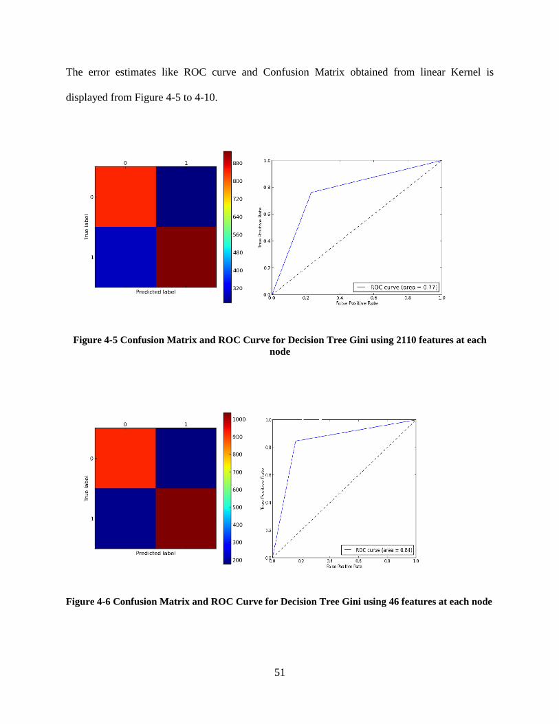
51
The error estimates like ROC curve and Confusion Matrix obtained from linear Kernel is
displayed from Figure 4-5 to 4-10.
Figure 4-5 Confusion Matrix and ROC Curve for Decision Tree Gini using 2110 features at each
node
Figure 4-6 Confusion Matrix and ROC Curve for Decision Tree Gini using 46 features at each node

52
Figure 4-7 Confusion Matrix and ROC Curve for Decision Tree Gini using 11 features at each node
Figure 4-8 Confusion Matrix and ROC Curve of Decision Tree Entropy using 2110 features at each
node

53
Figure 4-9 Confusion Matrix and ROC Curve of Decision Tree Entropy using 46 features at each
node
Figure 4-10 Confusion Matrix and ROC curve of Decision Tree Entropy using 11 features at each
node
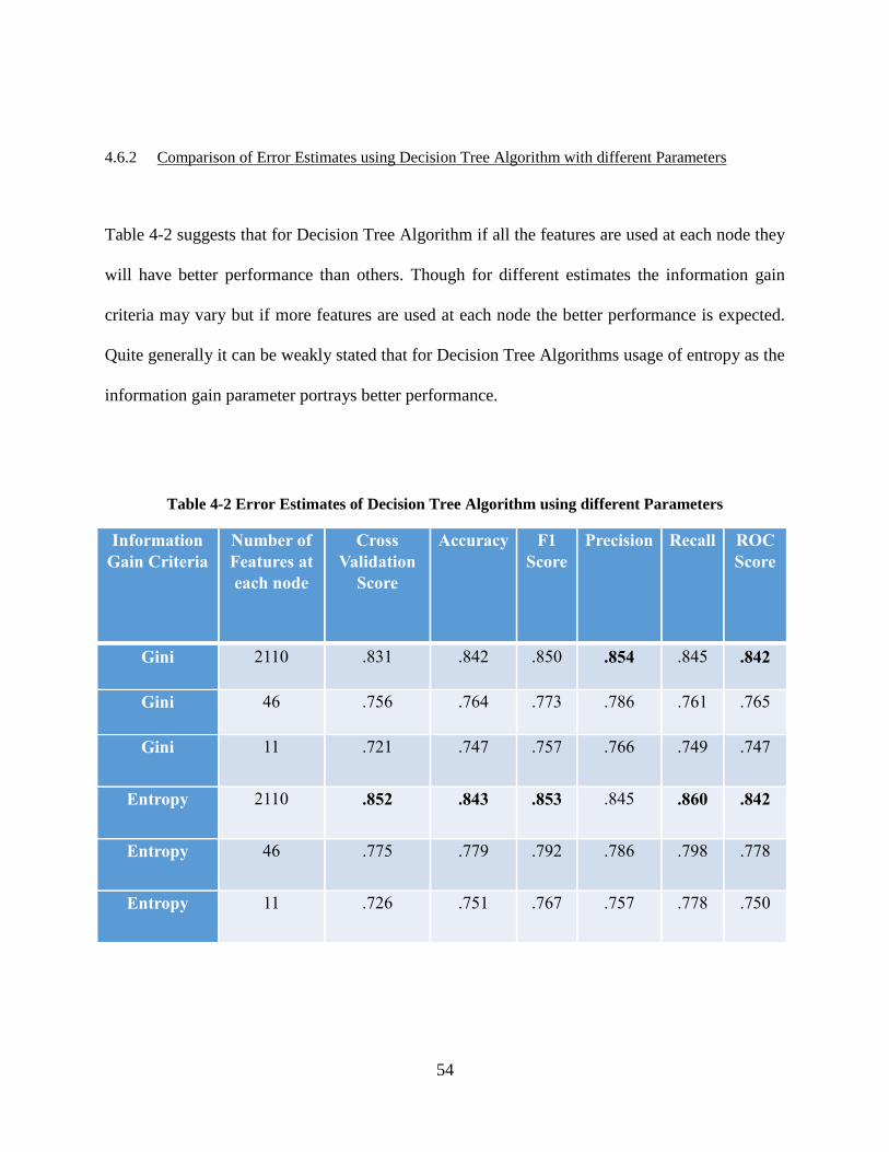
54
4.6.2 Comparison of Error Estimates using Decision Tree Algorithm with different Parameters
Table 4-2 suggests that for Decision Tree Algorithm if all the features are used at each node they
will have better performance than others. Though for different estimates the information gain
criteria may vary but if more features are used at each node the better performance is expected.
Quite generally it can be weakly stated that for Decision Tree Algorithms usage of entropy as the
information gain parameter portrays better performance.
Table 4-2 Error Estimates of Decision Tree Algorithm using different Parameters
Information
Gain Criteria
Number of
Features at
each node
Cross
Validation
Score
Accuracy F1
Score
Precision Recall ROC
Score
Gini
2110 .831 .842 .850 .854 .845 .842
Gini
46 .756 .764 .773 .786 .761 .765
Gini
11 .721 .747 .757 .766 .749 .747
Entropy
2110 .852 .843 .853 .845 .860 .842
Entropy
46 .775 .779 .792 .786 .798 .778
Entropy
11 .726 .751 .767 .757 .778 .750
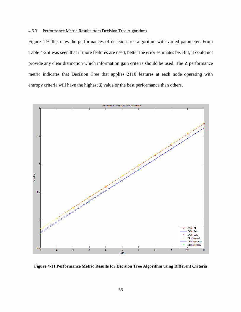
55
4.6.3 Performance Metric Results from Decision Tree Algorithms
Figure 4-9 illustrates the performances of decision tree algorithm with varied parameter. From
Table 4-2 it was seen that if more features are used, better the error estimates be. But, it could not
provide any clear distinction which information gain criteria should be used. The Z performance
metric indicates that Decision Tree that applies 2110 features at each node operating with
entropy criteria will have the highest Z value or the best performance than others.
Figure 4-11 Performance Metric Results for Decision Tree Algorithm using Different Criteria

56
4.7 Adaboost Algorithm
Adaboost Classifier is a meta-estimator. It begins with by fitting a classifier on the original
dataset. It then tries to fit additional copies of the classifier on the same dataset. In this step the
weights, which were incorrectly classified are adjusted such a way so that later classifiers can
concentrate more on difficult cases. It was first proposed by Freund et al. [Freund, 1999].
Adaboost algorithm is implemented using scikit-learn [Pedregosa, 2011] in python.
4.7.1 Parameters used in Adaboost Algorithm
The set of Parameters used in the Adaboost algorithm is illustrated below.
The error estimates like ROC curve and Confusion Matrix obtained from linear Kernel is
displayed from Figure 4-12 to 4-17.
Parameters in Adaboost Algorithm
1. Base Estimator= Decision Tree Classifier
2. Number of Estimators= 32, 64, 128,256, 512, 1024
3. Learning Rate =1
4. Algorithm=’SAMME’
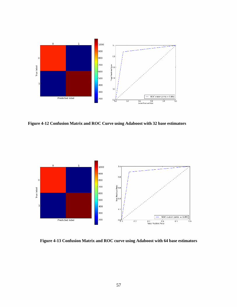
57
Figure 4-12 Confusion Matrix and ROC Curve using Adaboost with 32 base estimators
Figure 4-13 Confusion Matrix and ROC curve using Adaboost with 64 base estimators

58
Figure 4-14 Confusion Matrix and ROC Curve using Adaboost with 128 base estimators
Figure 4-15 Confusion Matrix and ROC Curve using Adaboost with 256 base estimators
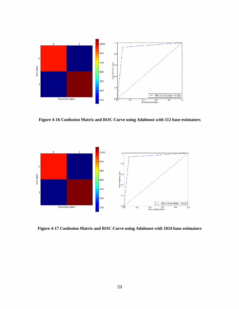
59
Figure 4-16 Confusion Matrix and ROC Curve using Adaboost with 512 base estimators
Figure 4-17 Confusion Matrix and ROC Curve using Adaboost with 1024 base estimators

60
4.7.2 Error Estimates from Adaboost Algorithm
Error estimates for Adaboost with different number of base estimators are listed in Table 4-3.
This indicates, the one with the highest base estimators will have better error estimate results.
This table also indicates that optimizations are not achieved. Because, if that would have
happened then Adaboost should have stopped earlier and there should have been some
convergence achieved in the results.
Table 4-3 Error Estimates from Adaboost Algorithm using different Base Estimators
Number of
Estimators
Cross
Validation
Score
Accuracy F1 Score Precision Recall ROC
Score
32
.883 .879 .885 .886 .884 .879
64
.895 .891 .897 .899 .894 .891
128
.906 .914 .918 .923 .914 .914
256
.911 .920 .924 .928 .920 .920
512
.910 .919 .923 .926 .920 .924
1024
.913 .926 .930 .933 .927 .926

61
4.7.3 Performance Metric Results on Adaboost Algorithm
Performance Metric results for Adaboost with different number of base Estimators are displayed
in Figure 4-14. From the performance metric the exact opposite result is noticed than in Table 4-
3. Here, highest Z value is achieved using the minimum of base estimators, in this case 32.
Figure 4-18 Performance Metric Result for Adaboost Algorithm using different Base Estimators

62
4.8 Random Forest Algorithm
A Random Forest Algorithm is an ensemble learning approach. It is also a meta-estimator. It fits
a number of decision tree classifiers on various sub-sections of the dataset. It uses an averaging
in order to improve the predictive accuracy and to control over-fitting. Random Forest Algorithm
was first proposed by Breiman et al. [Breiman, 2001].
4.9 Evaluation of Dataset to select range of Number of Trees
For a random forest algorithm a very basic question is “How many numbers of trees should be
used in a Random Forest”? Oshiro et al. [Oshiro, 2012] proposed a density based metric that is
used to quantify the quality of a dataset. Using that metrics an estimation of the number of trees
are also approximated. This thesis also follows the similar approach to quantify the quality of the
dataset and select a range of number of decision trees for random forest algorithm.
𝐷1 = 𝑙𝑜𝑔𝑎𝑛 = 1.112 … … (4.7)
𝐷2 = 𝑙𝑜𝑔𝑎
𝑛𝑐
= 1.022 … … (4.8)
𝐷3 = 𝑙𝑜𝑔𝑎
𝑛+1𝑐+1
= .9621 … … (4.9)
Here,
a= number of features=2110
c=number of classes=2
n= number of training examples=5000

63
According to Oshiro et al. [Oshiro, 2012] if the value of the density based metrics are greater
than 1 then the dataset can be classified easily, which is our case for first two metrics. But, for
the last one it is less than 1. So, we start with a tree number of 32 and double the number of trees
every time unless we see some convergence in their error estimates.
4.9.1 Weighted random Forest Algorithm used in this Method
In this method a weighted random forest algorithm is used to improve the predictive
performance. According to Winham et al.[Winham, 2013] Weighted random forest algorithm has
significant improvement in prediction over un-weighted random forest algorithm. In this method
a weight is defined such a way so that it can also give enough emphasize to the feature that has
more distinctive properties. The weight, w is defined as
𝑤 = 𝑛𝑣 × 𝑓𝑠𝑎𝑣𝑔… … (4.10)
Here,
𝑤 =weight
𝑛𝑣 = Number of majority votes for a class
𝑓𝑠𝑎𝑣𝑔= average score of the most important features
The weighted random forest algorithm is implemented using the un-weighted random forest code
,librf, a C++ implementation of original Random Forest proposed by Breiman et al. [Breiman,
2001], developed by Lee et al. [Lee, 2007].

64
4.9.2 Parameters used in Random Forest Algorithm
The set of Parameters used in Random Forest Algorithm is illustrated below.
4.9.3 Error Estimate Results from Random Forest Algorithm using Gini
The error estimates like ROC curve and Confusion Matrix obtained from Random Forest
Algorithm using Gini Criteria are displayed in the Figure 4-19 to 4-30.
Figure 4-19 Confusion Matrix and ROC Curve of Random Forest Gini using 32 Trees and 46
features at each node
Parameters in Random Forest Algorithm
1. Number of Estimators=32,64,128,256,512,1024
2. Maximum Depth=None
3. Minimum Samples Split=2
4. Minimum Samples at Leaf Node=None
5. Maximum Leaf Nodes=None
6. Information Gain Criteria= Gini, Entropy
7. Maximum Features at each node= 46,11
8. Bootstrapping= On
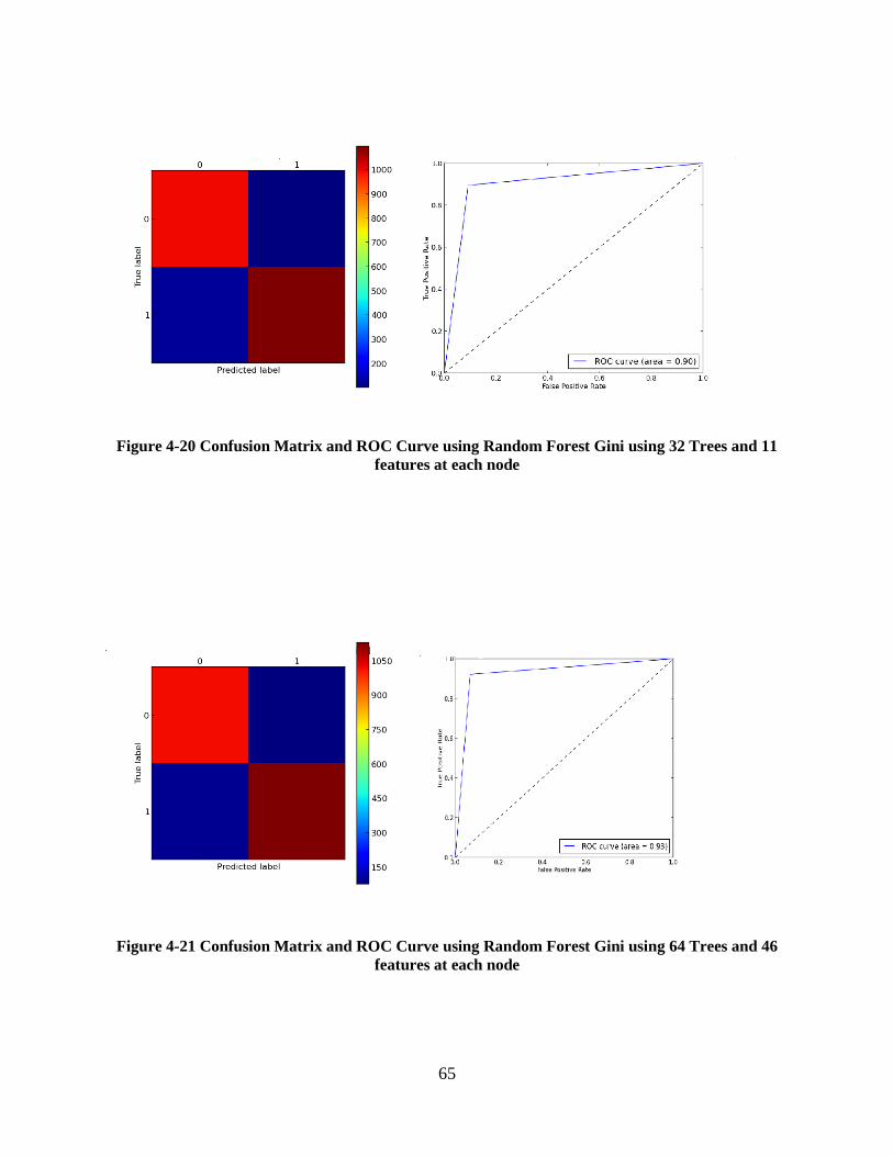
65
Figure 4-20 Confusion Matrix and ROC Curve using Random Forest Gini using 32 Trees and 11
features at each node
Figure 4-21 Confusion Matrix and ROC Curve using Random Forest Gini using 64 Trees and 46
features at each node

66
Figure 4-22Confusion Matrix and ROC Curve using Random Forest Gini using 64 Trees and 11
features at each node
Figure 4-23 Confusion Matrix and ROC Curve using Random Forest Gini using 128 Trees and 46
features at each node

67
Figure 4-24 Confusion Matrix and ROC Curve using Random Forest Gini using 128 Trees and 11
features at each node
Figure 4-25 Confusion Matrix and ROC Curve using Random Forest Gini using 256 Trees and 46
features at each node

68
Figure 4-26 Confusion Matrix and ROC Curve using Random Forest Gini using 256 Trees and 11
features at each node
Figure 4-27 Confusion Matrix and ROC Curve using Random Forest Gini using 512 Trees and 46
features at each node
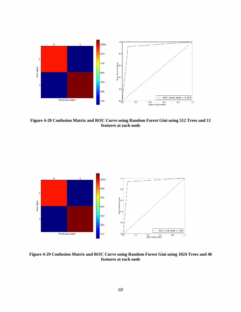
69
Figure 4-28 Confusion Matrix and ROC Curve using Random Forest Gini using 512 Trees and 11
features at each node
Figure 4-29 Confusion Matrix and ROC Curve using Random Forest Gini using 1024 Trees and 46
features at each node

70
Figure 4-30 Confusion Matrix and ROC Curve using Random Forest Gini using 1024 Trees and 11
features at each node
Error Estimates for different Parameters of Random Forest Algorithm using Gini Information criteria are
compared in Table 4-4. It can be stated that best error estimates are achieved as higher number of trees are
used and with higher number of features at each node. It is also noted that, it tends to converge at some
point which indicates, growing trees beyond that would not be wise.

71
Table 4-4 Error Estimates obtained for different parameters of Random Forest Algorithm using
Gini Criteria
Informa
tion
Gain
Criteria
Number
of Trees Number
of
Features
at each
node
Out of
Bag
Score
Accurac
y F1 Score Precisio
n Recall ROC
Score
Gini
Index
32
46
.885 .915 .918 .931 .906 .915
11
.861 .901 .905 .915 .895 .901
64 46
.902 .925 .929 .936 .921 .926
11
.881 .904 .909 .916 .902 .905
128 46
.913 .928 .931 .934 .928 .928
11
.901 .912 .916 .920 .911 .912
256 46
.921 .927 .930 .934 .927 .927
11
.906 .907 .919 .923 .924 .918
512 46
.921 .933 .936 .940 .935 .935
11
.906 .916 .920 .924 .915 .916
1024 46
.923 .935 .939 .940 .935 .935
11
.911 .919 .923 .926 .920 .919
4.9.4 Error Estimate Results from Random Forest Algorithm using Entropy Criteria
The error estimates like ROC curve and Confusion Matrix obtained from Random Forest
Algorithm using Entropy Criteria are displayed in Figure 4-31 to 4-42.

72
Figure 4-31 Confusion Matrix and ROC Curve of Random Forest Entropy with 32 trees using 46
features at each node
Figure 4-32 Confusion Matrix and ROC Curve of Random Forest Entropy with 32 trees using 11
features at each node

73
Figure 4-33 Confusion Matrix and ROC Curve of Random Forest Entropy with 64 trees using 46
features at each node
Figure 4-34 Confusion Matrix and ROC Curve of Random Forest Entropy with 64 trees using 11
features at each node

74
Figure 4-35 Confusion Matrix and ROC Curve of Random Forest Entropy with 128 trees using 46
features at each node
Figure 4-36 Confusion Matrix and ROC Curve of Random Forest Entropy with 128 trees using 11
features at each node
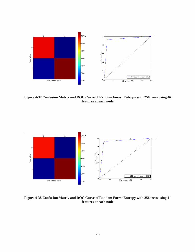
75
Figure 4-37 Confusion Matrix and ROC Curve of Random Forest Entropy with 256 trees using 46
features at each node
Figure 4-38 Confusion Matrix and ROC Curve of Random Forest Entropy with 256 trees using 11
features at each node

76
Figure 4-39 Confusion Matrix and ROC Curve of Random Forest Entropy with 512 trees using 46
features at each node
Figure 4-40 Confusion Matrix and ROC Curve of Random Forest Entropy with 512 trees using 11
features at each node

77
Figure 4-41 Confusion Matrix and ROC Curve of Random Forest Entropy with 1024 trees using 46
features at each node
Figure 4-42 Confusion Matrix and ROC Curve of Random Forest Entropy with 1024 trees using 11
features at each node
Error Estimates for different Parameters of Random Forest Algorithm using Entropy Criteria are
compared in Table 4-5. From Table 4-5 it is observed that best error estimates are achieved with

78
higher number of trees and they also tend to converge at some point (after 256 trees, more
evident after 512 trees).
Table 4-5 Error Parameters obtained for different parameters of Random Forest Algorithm using
Entropy Criteria
Informa
tion
Gain
Criteria
Number
of Trees Number
of
Features
at each
node
Out of
Bag
Score
Accurac
y F1 Score Precisio
n Recall ROC
Score
Entropy
32
46
.887 .919 .922 .933 .911 .919
11
.855 .904 .908 .921 .895 .904
64 46
.903 .926 .929 .936 .923 .926
11
.885 .908 .912 .919 .906 .908
128 46
.886 .915 .918 .934 .902 .916
11
.893 .913 .917 .932 .902 .914
256 46
.917 .931 .934 .943 .925 .931
11
.905 .918. .922 .928 .916 .918
512 46
.921 .923 .926 .931 .922 .932
11
.913 .923 .926 .931 .922 .933
1024 46
.921 .932 .935 .944 .926 .932
11
.906 .919 .923 .929 .916 .919

79
4.9.5 Performance Metric Results from Random Forest Algorithm with Different Number of Trees
Performance Metric results for Random Forest Algorithm using different number of Trees are
displayed from Figure 4-43 to Figure 4-48.
4.9.5.1 Random Forest with 32 Trees
When comparing the error estimates it was observed that best results were achieved with higher
number of features at each node. But, here it can be seen that with Entropy gain criteria and 11
features at each node best performance is achieved.
Figure 4-43Comparison of Performance Metric Results of Random Forest Algorithm using 32
Trees
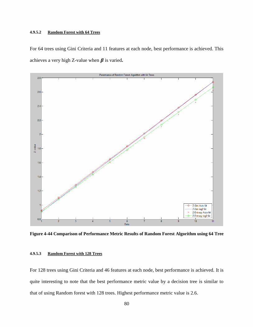
80
4.9.5.2 Random Forest with 64 Trees
For 64 trees using Gini Criteria and 11 features at each node, best performance is achieved. This
achieves a very high Z-value when 𝜷 is varied.
Figure 4-44 Comparison of Performance Metric Results of Random Forest Algorithm using 64 Tree
4.9.5.3 Random Forest with 128 Trees
For 128 trees using Gini Criteria and 46 features at each node, best performance is achieved. It is
quite interesting to note that the best performance metric value by a decision tree is similar to
that of using Random forest with 128 trees. Highest performance metric value is 2.6.

81
Figure 4-45 Comparison of Performance Metric Results of Random Forest Algorithm using 128
Trees
4.9.5.4 Random Forest with 256 Trees
For 256 trees using Gini Criteria and 11 features at each node best performance is achieved.
With 256 trees for almost all parameters the performance metric degrades in comparison with
number of trees fewer than 256. It is believed that this is the starting point where a large number
of decision trees start to generate heavy computational effect which is responsible for
performance degradation.
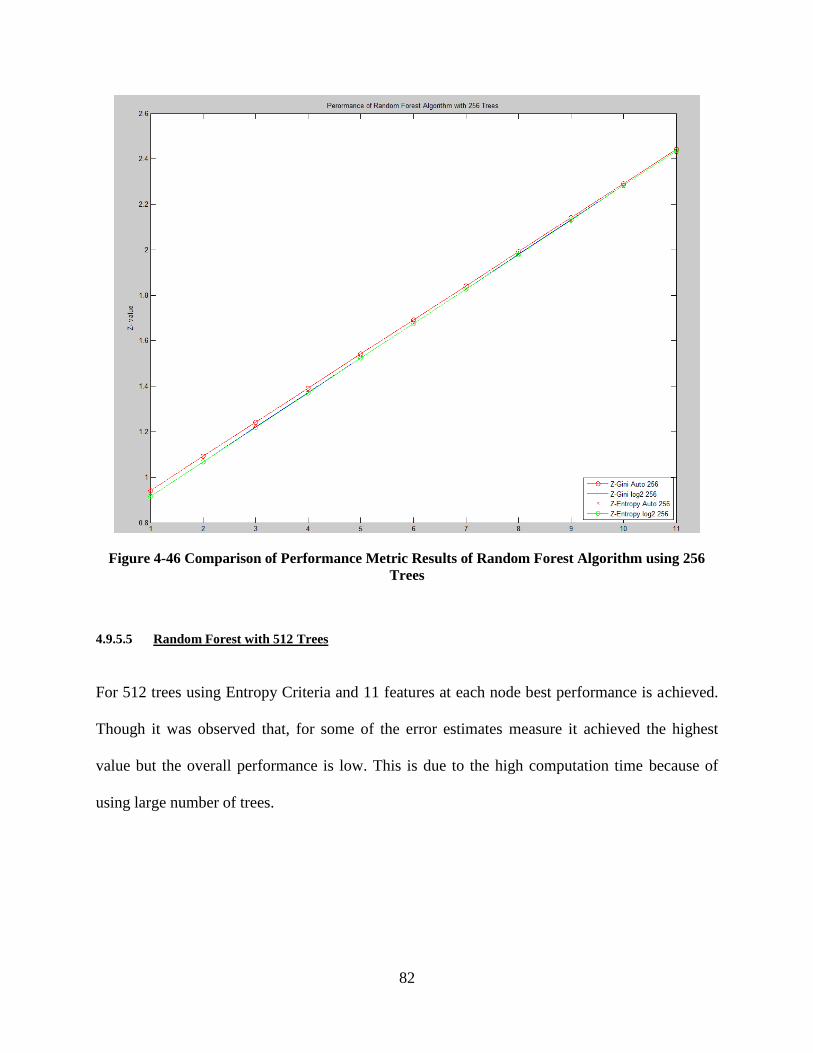
82
Figure 4-46 Comparison of Performance Metric Results of Random Forest Algorithm using 256
Trees
4.9.5.5 Random Forest with 512 Trees
For 512 trees using Entropy Criteria and 11 features at each node best performance is achieved.
Though it was observed that, for some of the error estimates measure it achieved the highest
value but the overall performance is low. This is due to the high computation time because of
using large number of trees.
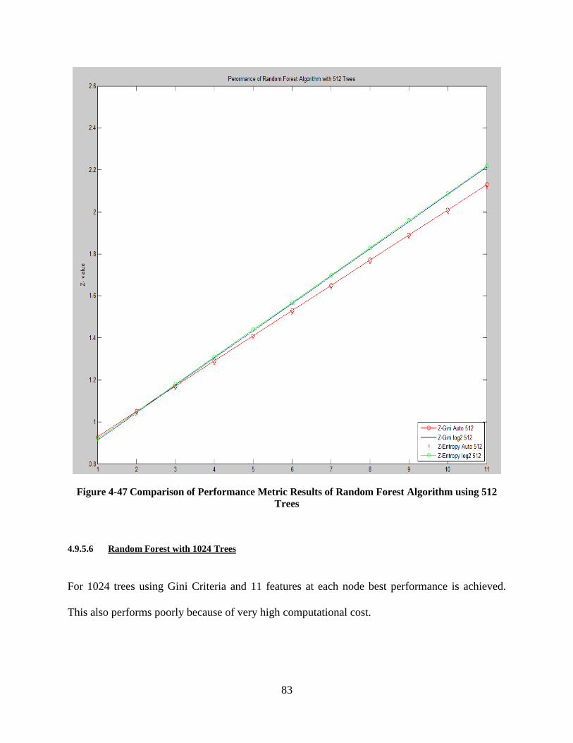
83
Figure 4-47 Comparison of Performance Metric Results of Random Forest Algorithm using 512
Trees
4.9.5.6 Random Forest with 1024 Trees
For 1024 trees using Gini Criteria and 11 features at each node best performance is achieved.
This also performs poorly because of very high computational cost.

84
Figure 4-48 Comparison of Performance Metric Results of Random Forest Algorithm using 1024
Trees
4.10 Selection of the Best Algorithm with Optimal Parameters
The best algorithm is selected based on the value of Z at highest 𝜷 value. For each algorithm the
best one with optimal parameter is selected and their values are compared.

85
Table 4-6 Selection of Best Algorithm with Optimal Parameters
Algorithm with Best Parameter Highest Z- Value
Linear SVM 2.1 (Range= 0.9-2.1)
Decision Tree (Entropy, 2110 features at each
node)
2.5 (Range= 0.9-2.5)
Adaboost (32 base estimators) 1.6 (Range= 0.8-1.6)
Weighted Random Forest (Gini, 11
features at each node, 64 Trees)
2.7 (Range= .9-2.7)
So, it can be seen from Table 4-6 that Weighted Random Forest with Gini criteria, 11 features at
each node and 64 trees has highest Z- value= 2.7. So, this algorithm will be used for developing
Grasping Algorithm in this system.
4.11 Selection of Most Significant Features
Earlier to this chapter, a feature extraction technique was employed that yielded 2110 features.
Using so many features is computationally very expensive. That is why a variable importance
method is employed to reduce the feature space. Using the variable importance technique
discussed by Breiman et al. [Breiman, 2001] the feature space is reduced.
Scores were extracted for each variable (feature). The following procedure was followed to
select the most important variables based on their scores

86
Figure 4-49 Important Variable Selection Algorithm
Start
Compute the score of the features,
𝐹𝑠 using variable importance
Compute the mean score, 𝑚𝑠 of all
the features
Is 𝐹𝑠 − 𝑚𝑠 > .2
Current Feature
Number=1
Consider it
Finish
Is Current feature Number=
Maximum Feature Number?
Discard
it
Current Feature
Number=Current
Feature Number
+1
No
Yes
No
Yes
87
In this way total 715 features are selected. The grasping algorithm is trained and tested using
these 715 features. So, the parameters of the best algorithm is as follows
4.12 References
T. M. Oshiro, P. S. Perez, J. A. Baranaukas. Lecture notes in Computer Science, 2012, DOI:10.
1007/978-3-642-31537-4_13
L. Breiman. Machine Learning, 45, 5-32, 2001.
Y. Freund, R. E. Schapire. A Short Introduction to Boosting. Journal of Japanese Society for
Artifical Intelligence, 14 (5): 771-780, September, 1999.
J. R. Quinlan. Introduction of Decision Trees. Machine Learning 1: 81-106, 1986.
Selected Algorithm (Weighted Random Forest) with optimal parameters
1. Number of Estimators=64
2. Maximum Depth=None
3. Minimum Samples Split=2
4. Minimum Samples at Leaf Node=None
5. Maximum Leaf Nodes=None
6. Information Gain Criteria= Gini
7. Maximum Features at each node= 𝑙𝑜𝑔2 (715)=10
8. Bootstrapping= Off

88
B. Lee, librf: A library for random forests, 2007, http;//mtv.ece.ucsb.edu/benlee/librf.html
S. J. Winham, R. R. Freimuth, J. M. Biernacka. A Weighted Random Forest Approach to
Improve Predictive Performance, 2013. Stat Anal Data Min, 6(6): 496-505. Doi:
10.1002/sam.11196
V. Vapnik, C. Cortes. Support Vector Networks. Machine Learning. Vol. 20. Issue 3. Pp. 273-
297, 1995
F. Pedregosa et al. Scikit-Learn: Machine Learning in Python. JMLR 12, pp. 2825-2830, 2011.
S. Ali, K. A. Smith. On Learning Algorithm Selection for Classification. Applied Soft
Computing 6 (2006) 119-138.

89
CHAPTER 5: GRASPING ALGORITHM
5.1 Introduction
The grasping algorithm developed in this system takes a 2-D image and an aligned depth map of
the object to be grasped as the input and outputs a rectangular region on the 2-D image that
corresponds to the best grasping rectangular region as determined by the system. The input is
referred as a single image with four values at each pixel-RGBD-where D represents the depth.
There will be a lot of rectangles on an object which will correspond to a valid grasping rectangle.
The goal of this method is to find the optimal grasping rectangle on the object. This method is
motivated by Jiang et al. [Jiang, 2011]. The score function definition and the design of grasping
algorithm are extracted from Jiang et al. [Jiang, 2011]. This method differs from the above
mentioned method in terms of the number of features used to calculate the score function and
weight, w is learned from a weighted random forest algorithm instead of svm-rank proposed
there. For the purpose of better understanding definition of score function, fast search procedure
and algorithm iteration steps are described here too from Jiang et al. [Jiang, 2011]. Code for
grasping with rectangle representation by Jiang et al. [Jiang, 2011] is used and integrated with
weighted random forest algorithm that learns from selective image and point cloud feature.
The selection of the optimal rectangle is done using a score function quantitatively. So, the aim is
to find out a rectangle that has the highest score. The score function is defined using the feature
values of a rectangle which is described later in detail in this chapter. To compute the score
function of a rectangle, it is needed to consider all the rectangles on an image. It is quite
infeasible to perform an exhaustive search on an image that takes into account all the rectangles.

90
The computational complexity will be huge and the system will not be of practical use. As, the
present system aims at development of a method that will replace human operators in regular
setting and serve the basic purposes of assistive robotics, it is needed to consider an approach
that will perform this score function computation as fast as possible.
In order for fast computation of a score function this methods uses an approach that computes
both the score and the feature values in an incremental fashion. This method of computing score
function narrows down the search space significantly. In order to meet this requirement some
more computationally expensive features need to be avoided from the feature extraction step.
This also poses another problem of losing more informative feature that carries higher
significance. So, a trade-off is needed to balance off between the accuracy and speed of the
grasping system. This challenge is addressed in this method by the use of a two-step process as
in Jiang et al. [Jiang, 2011].
In the first step, features which allow incremental computation of the score function are used.
Features like Color, Edge, Texture, Depth, Surface Normal, Curvature, and View Point Feature
Histogram Descriptors fall to this category. Usage of these features allows reducing the search
space from tens of millions down to hundred rectangles. Then in the second-step, more
exhaustive and sophisticated features are used and the optimal rectangle is captured. All the non-
linear features used in this method are applied in this step. Here the first step is little inaccurate
but very fast while the second-step is more accurate and little slow. This chapter deals with the
detailed description of the grasping algorithm, implementation of the method and demonstrates

91
the training and testing results obtained from University of Central Florida Computational
Control Systems Laboratory and Cornell University Personal Robotics Dataset.
5.2 Chapter Objectives
Definition of the Score Function.
Computation of Score Function in an Incremental Fast Search Procedure.
Design of the Grasping Algorithm.
Training the system that enables learning to select a grasping rectangle on an object.
Testing of the system.
Demonstration of Experimental Results on Cornell University Dataset
Demonstration of Experimental Results on Central Florida Computational Control
Systems Laboratory Dataset
Analyze the System Performance using an Evaluation Metric.
5.3 Learning a Score Function
5.3.1 Definition of a Score Function
Let, a rectangle is denoted by G and its corresponding score function is denoted by 𝐟(𝐆). The
goal of this method is to find an optimal rectangle, G* that has the maximum score value. This
can be numerically demonstrated as
𝐺∗ = 𝑎𝑟𝑔 𝑚𝑎𝑥𝐺 𝑓(𝐺) … … (5.1)
Score function, 𝐟(𝐆) can be defined as
𝑓(𝐺) = 𝑤𝑇⏀(𝐺) = ∑ 𝑤𝑖
𝑖=𝑘
𝑖=1⏀𝑖(𝐺) … … (5.2)
Here, 𝑓 is defined as a linear function of features. This is quite a common technique for machine
learning algorithms [Cortes, 1995]. In addition to that, it also allows the method to be simple.
This also ensures that the search process is accelerated which is discussed later. ⏀(𝑮) denotes
92
the feature value of a rectangle G. 𝒘 denotes the weight which is learned using Weighted
Random Forest Algorithm. This similar technique is motivated by other researchers. In those
methods they showed that generalization is achieved using some sort of learning algorithms. This
is more robust than some hand-written rules or manually computed parameters for a few
features.
In our supervised Random Forest Algorithm, we noted that there will always be more than one
good grasp on an object. But, among them one or some will be more desirable. These will
provide more robustness into the system and allow performing manipulation on the object. This
provides a distinction between a good grasp and a bad grasp but still does not provide the exact
separation. That is why this method focuses on ranking the grasping regions based on the
attributes used rather than classifying the good and bad grasping regions. The one that has the
highest score is considered to be of rank 1.
5.3.2 Computing of a Score Function
In a view to find the rectangle that has the highest score performing exhaustive search method to
compute score value of all the rectangles is quite expensive and infeasible. This method comes
into action in case of finding a suitable grasping point. But for searching a rectangle with highest
score this method uses a definitive fast search approach. Here, the problem of finding the highest
score is similar to the very classic problem of finding the maximum-sum sub matrix [Bentley,
1984]. To compute maximum sum sub matrix various efficient algorithms are presently
available. In order to solve the problem more efficiently the score value of each rectangle is

93
decomposed as a sum of scores of each pixel in that rectangle [Jiang, 2011]. The usage of the
linear function while defining the score, facilitates in achieving this decomposition of score as
the sum of scores of individual pixels. Now, the problem is also less complex. It needs to find the
score value at each pixel on a rectangle. Then the sum of those values is the score of that
rectangle.
5.3.3 Assumption
Let, the score function f(G) of a rectangle G is known. We assume the features are additive.
Numerically it is illustrated as,
𝑖(G ∪△ G) =
𝑖 (𝐺) + 𝑖(△ 𝐺) … … (5. 3)
Let, 𝐺′ = 𝐺 ∪△ G. Then, the score of the new rectangle 𝐺′can easily be computed as,
𝑓(𝐺′) = 𝑓(𝐺 ∪△ 𝐺) … … (5.4)
It can be further expanded as,
𝑓(𝐺′) = ∑ 𝑤𝑖𝑖=1
𝑖=𝑘
𝑖(𝐺 ∪△ 𝐺) = 𝑓(𝐺) + 𝑓(△ 𝐺) … … (5.5)
So, this method needs to only compute, 𝐟(△ 𝐆) only instead of computing for the entire
rectangle. This way, search space is reduced significantly and allows the computational speed to
be very fast.
Here, the feature value ⏀(𝐆) can be simplified as,

94
𝑖(𝐺) = ∑
𝑖(𝑥,𝑦)∈𝐺
(𝐼(𝑥, 𝑦)) … … (5.6)
This indicates that feature value, ⏀(𝐆) at each rectangle is determined as the sum of feature
values at each pixel.
5.3.4 Incremental Search Procedure
The incremental search process allows computing the score of all the rectangles in an extensively
fast manner. This is described in using the expansion of the score function below. This is a
method extracted from Jiang et al. [Jiang, 2011] and proposed by Joachims et al. [Joachims,
2002]. Let, we want to compute the score function, 𝐟(𝐆) of rectangle G from k number of
features.
𝑓(𝐺) = ∑ 𝑤𝑖𝑖
𝑖=𝑘
𝑖=1
(𝐺) … … (5.7)
So, 𝑓(𝐺) was defined as the sum of the products of weight and feature value for all the features.
𝑓(𝐺) = ∑ ∑𝑥=𝑟𝐺
𝑥=𝑟𝐺+𝑛𝐺 𝑖=1
𝑖=𝑘
∑ 𝑤𝑖𝑖(𝐼(𝑥, 𝑦))
𝑦=𝑐𝐺
𝑦=𝑐𝐺+𝑚𝐺
… … (5.8)
𝐟(𝐆), can also be written this way. Here x indicates the range of rows and y indicates the range of
columns. Feature value of a rectangle, ⏀(𝐆) is expanded as it is the summation of feature value
at each pixel (x, y) in image I. After interchanging we get,
𝑓(𝐺) = ∑𝑥=𝑟𝐺
𝑥=𝑟𝐺+𝑛𝐺 ∑ ∑ 𝑤𝑖𝑖=1
𝑖=𝑘
𝑖(𝐼(𝑥, 𝑦)) … … (5.9)𝑦=𝑐𝐺
𝑦=𝑐𝐺+𝑚𝐺

95
𝑓(𝐺) = ∑𝑥=𝑟𝐺
𝑥=𝑟𝐺+𝑛𝐺 ∑𝑦=𝑐𝐺
𝑦=𝑐𝐺+𝑚𝐺 𝐹(𝑥, 𝑦) … … (5.10)
Here, a new function 𝐅(𝐱, 𝐲) is defined, which indicates the score value at each pixel (x, y). So,
the algorithm is shown in Figure 5-1
.
Figure 5-1 Incremental Fast Search Algorithm Used in this System
5.4 Background Subtraction using Mixture of Gaussian Model
Background Subtraction is one of the significant preprocessing steps in grasping region
selection. For this method it is assumed that when the system will be implemented in practice
there will be some computer vision algorithm available to address this issue. As this method
96
entirely focuses on implementation of a grasping rectangle selection for any novel object using
Random Forest Algorithm so, a simple background subtraction algorithm is used here. This
Approach is followed being inspired by Lim et al. [Lim, 2010]. In order to use such background
subtraction algorithm, a 2D image of the scene without the object is also used along with the 2D
image of the object as input. This method facilitates the use of a simple Mixture of Gaussian
Background Subtraction Algorithm in OpenCV [Bradski, 2000]. The result is shown in Figure 5-
2.
Mixture of Gaussian Background/Foreground Segmentation Algorithm was used for background
subtraction. Here, a method is used that models each background pixel by a mixture of k
Gaussian distributions. K value is used as 5. The weights in the mixture represent the time
proportions. This indicates that those colors stay in the scene. The colors which are more static
and stay for long are the probable background colors.

97
Figure 5-2 Background Subtraction result using Mixture of Gaussian subtraction Algorithm. The
top left image is background, the one on the right is the image of the object and the bottom image
illustrates the foreground mask after subtracting the background from the foreground
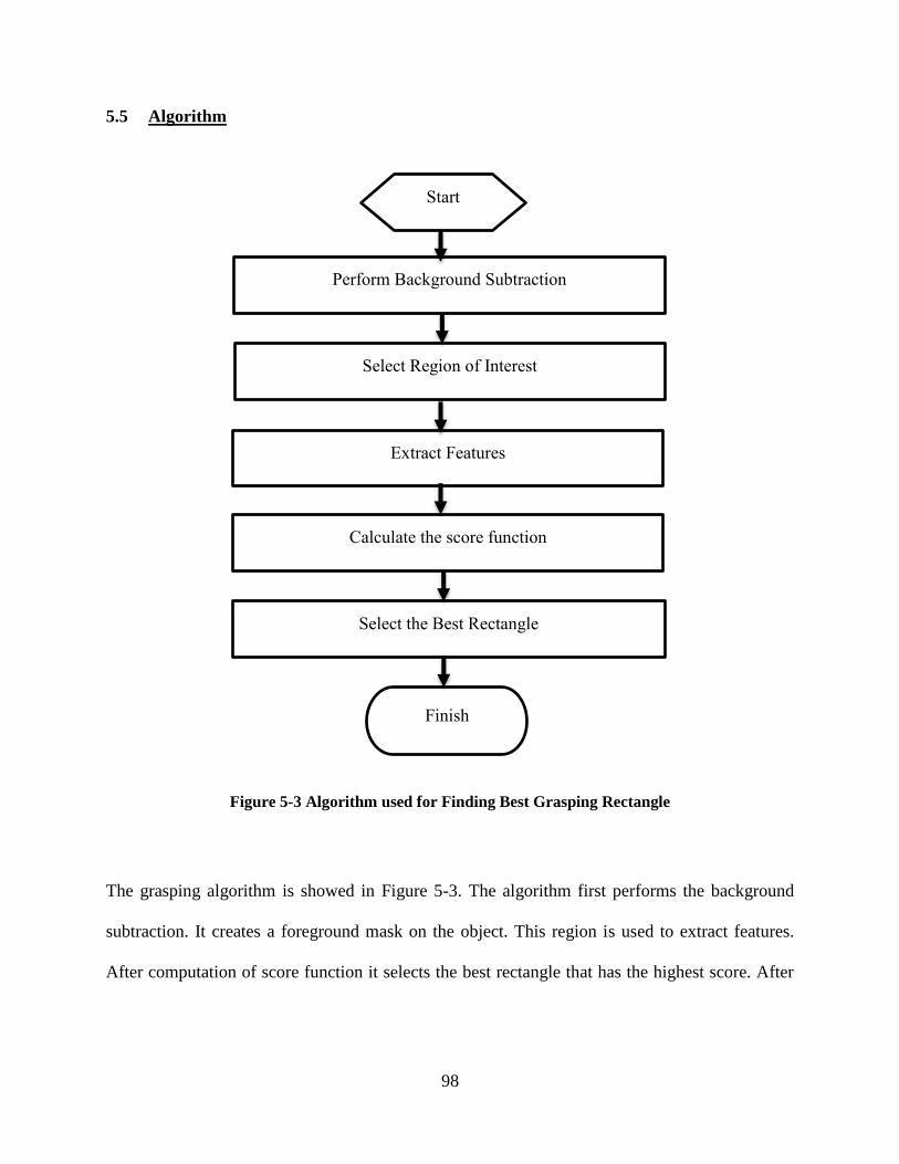
98
5.5 Algorithm
Figure 5-3 Algorithm used for Finding Best Grasping Rectangle
The grasping algorithm is showed in Figure 5-3. The algorithm first performs the background
subtraction. It creates a foreground mask on the object. This region is used to extract features.
After computation of score function it selects the best rectangle that has the highest score. After
Start
Perform Background Subtraction
Select Region of Interest
Extract Features
Calculate the score function
Select the Best Rectangle
Finish

99
the entire sequence is completed for an orientation the image is rotated 20 degrees with the
image plane and performed again until 360 degrees.
5.6 Hardware Setup
This method is intended to be used for grasping novel objects using Parallel plate Gripper of
Baxter Research Robot by Rethink Robotics Inc.. Baxter Head Camera was used for capturing
the 2D image of the object. The resolution of the image is 640 x 400, has a frame rate of 30
frames per second and focal length of 1.2 mm. In order to capture the point cloud Baxter Head
Sonar ring was used. The algorithm was implemented in a 2.6 GHz Intel Core i5 processor that
uses Virtual Box with 32 bit Ubuntu 10.04 and 4GB RAM.
5.7 Evaluation Metric
In order the implemented grasp to be successful it needs to satisfy several criteria. In this method
the criterions are used from Jiang et al. [Jiang, 2011] and Saxena et al. [Saxena, 2006]. The same
criterions are followed in the evaluation metric like these approaches but this method imposed
more stringent conditions on the metric. The criterions followed in the above methods are
described below:
The centroid of the Parallel Plate Gripper should be at the correct location.
All of the three orientation angles should be correct.
The area should have sufficient width so that the Parallel Plate Gripper can be placed
while performing the grasping.

100
These factors have a mutual interplay between them. One center point will not work for all the
orientations [Jiang, 2011]. The evaluation metric used in this method uses both Point Metric and
Rectangle Metric to measure the performance of the algorithm.
5.7.1 Point Metric
In this method a Rectangular Region is used for prediction. At first, the center of the rectangle is
computed. If the distance of the center of the rectangle is within a certain threshold in
comparison with the ground truth rectangle, then it is considered to a correct prediction using as
described in Point Metric [Saxena, 2006].
5.7.2 Rectangle Metric
Let us consider, G is the predicted Rectangle and G* is the Ground Truth Rectangle. For our
performance analysis we made some modification in the evaluation metric algorithm and
introduced some stringent conditions. These are discussed below:
First Pass: If the predicted Rectangle G has an orientation difference of greater than 20
degrees with ground truth rectangle G* then it will be considered as incorrect prediction.
Second Pass: If the amount of area of overlap between G and G* are less than 30% then
this also falls to the incorrect prediction category.
In case of multiple grasping rectangles each one is considered and evaluated. The one
with the best result (maximum area overlap and minimum orientation difference) is used
for the computation of the system performance.

101
5.8 Experimental Results
In this method Training is performed on the Cornell University Grasping Dataset. The system is
tested on both Cornell University Dataset and Computational Control Systems Laboratory at
University of Central Florida Dataset.
5.9 Training Dataset
Cornell University Personal Robotics Dataset is used for Training. In this method out of 285
objects 200 objects were used for Training. A sample of the dataset is illustrated in Figure 5-4,
which is collected from Cornell University Website.
Figure 5-4 Screenshot of Some Objects of Cornell University Personal Robotics Dataset from
Personal Robotics Website used for Training
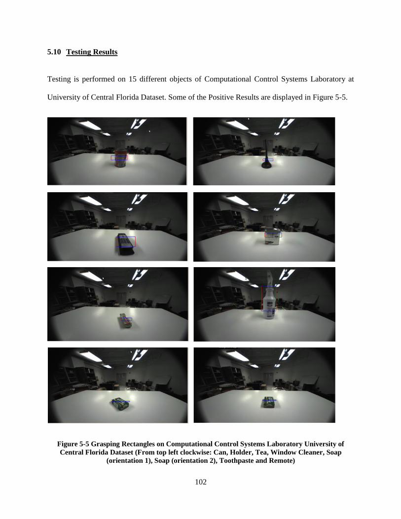
102
5.10 Testing Results
Testing is performed on 15 different objects of Computational Control Systems Laboratory at
University of Central Florida Dataset. Some of the Positive Results are displayed in Figure 5-5.
Figure 5-5 Grasping Rectangles on Computational Control Systems Laboratory University of
Central Florida Dataset (From top left clockwise: Can, Holder, Tea, Window Cleaner, Soap
(orientation 1), Soap (orientation 2), Toothpaste and Remote)

103
Table 5-1 Result on Cornell University Dataset
Dataset Object Specific
Training
Two Step RGBD
(Image + Point
Cloud + FPFH)
Features
Prediction Rate
(%)
General Training
Two Step RGBD
(Image + Point
Cloud + FPFH)
Features
Prediction Rate
(%)
Object Specific
Training
Two Step RGBD
(Image + Point
Cloud + VFH)
Features
Prediction Rate
(%)
General
Training
Two Step RGBD
(Image + Point
Cloud + VFH)
Features
Prediction Rate
(%)
Remote 88.4 91.6 80 88
Marker 91.2 86.2 91.4 89.6
Pencil Bag 76.4 74 81.2 72.8
Bulb 82.4 84.4 82.4 78.6
Screwdriver 100 80 100 100
Brush 100 82.4 100 92.4
Lid 61.2 56 71.3 60.4
Box 56.8 33.2 60.5 57.9
Shoe 34.8 57.6 49 38.1
Average 76.8 72.68 79.2 75.2

104
Table 5-2 Result on Computational Control System Laboratory University of Central Florida
Dataset
Dataset Object Specific Training
Two Step RGBD
(Image+ Point Cloud+ VFH)
Features
Prediction Rate (%)
General Training
Two Step RGBD
(Image+ Point Cloud+ VFH)
Features
Prediction Rate (%)
Remote 100 100
Soap 100 100
Toothpaste 100 100
Camera 100 100
Can 100 100
Pen 100 100
Window Cleaner 100 100
Multimeter 0 0
Complex Penholder 100 0
Average 93.33 86.64

105
5.11 Discussion
This method uses 715 features to compute the score function. Out of these 715 features, 576 are
image features, 85 are point cloud features and 54 are VFH features. From Table 5-1, it is quite
evident that using VFH Features there is an increase in the algorithm performance than FPFH
features. From Table 5-1 it can also be seen that using VFH feature for object specific and
general testing there is an average of 2.46% performance increase is observed.
It can be seen from the above two charts that, the method performs better for UCF
Computational Control Systems Laboratory dataset than Cornell University Personal Robotics
Dataset. This may be due to large variability of objects used in Cornell dataset and contains more
complex shaped object. From UCF dataset result, it can be observed that mostly the rectangles
are aligned horizontally with respect to the image plane. So, it does not work very well for pose
estimation. But, it is very efficient in finding the suitable grasping rectangle from an unknown
object.
From Table 5-1 it is observed that it performs poorly in comparison with others for lid, boxes
and shoes. This method performs very well for Screwdriver, Toothbrush, Remote and Marker.
These are the type of objects where there is a large flat area can be found. It is very capable of
finding a good gasping region from these kinds of objects.

106
From Table 5-2 it is obvious that it performs well for some plain shaped objects but it fails for
multimeter and penholder. Though using object specific training for penholder performance is
increased, but it can never find a suitable grasping region on a multimeter. In Figure 5-6
unsuccessful results on UCF dataset is shown. For multimeter it finds a region on the wire, which
is not a valid grasping point as determined by the evaluation metric.
Figure 5-6 Unsuccessful grasping result on multimeter
Figure 5-7 Unsuccessful grasping result on a Penholder

107
The method developed in this dataset is computationally very fast. In a 32 bit machine it takes
24.80 seconds on an average to detect the grasping rectangle. Using a better configuration
machine will certainly improve the run time.
5.12 References
Y. Jiang, S. Moseson, and A. Saxena. Efficient Grasping from RGBD Images: Learning using a
new Rectangle Representation. ICRA, pp. 3304-331, 2011.
A. Saxena, J. Driemeyer and A. Ng. Robotic Grasping of Novel Objects using Vision. IJRR, vol.
27, no.2, Multimedia Archives, 2008, p. 157.
A. Saxena, J. Driemeyer, J. Kearns, and A.Y. Ng. 2006. Robotic grasping of novel objects:
NIPS, 2006.
J. Bentley. Programming Pearls: algorithm design techniques. Commun. ACM, vol. 27, no .9,
pp. 865-873, 1984.
A. Saxena, J. Driemeyer, J. Kearns, C. Osondu and A. Y. Ng, Learning to grasp Novel objects
using Vision, ISER, 2006.
G. Bradski, OPENCV_LIBRARY, Dr. Dobb’s Journal of Software Tools, 2000, 2236121.

108
T. Joachims. Optimizing Search Engines using clickthrough data. SIGKDD, 2002.
C. Cortes and V. Vapnik. Support Vector Networks. Machine Learning. Vol. 20, no. 3, pp 273-
297, 1995.

109
CHAPTER 6: CONCLUSION AND FUTURE SCOPE OF RESEARCH
6.1 Introduction
The principle focus of this method was to develop a system that can work beside human in day to
day settings. This method intended to find a grasping region that would ensure robust grasp. So,
it can be said that this method serves as a very efficient approach towards robotic manipulation
of objects. While developing the method, it also considered to make the system computationally
fast and reliable. This chapter focuses on providing a general overview of the developed system
and directs a pathway that will be followed to achieve the intended goal of assistive robotics in
future.
6.2 Chapter Objectives
Discussing the summary of the entire work
Discussion of the novel contribution in the field of Robotic Grasping Research proposed
and implemented in this thesis.
Discussion of the future scope of research using this approach.
6.3 Summary of the Grasping System
The grasping system developed in this method utilizing weighted random forest algorithm has
significantly high accuracy in detecting a rectangular grasping region on any unknown objects.
The method also has a significantly low run time and has every potential to be extended for a real
time system. Like all other supervised learning methods, this one can also be divided into two
parts: Training and Testing.
110
Here Training is performed offline. A feature extraction step is performed prior to training. This
can be considered as a pre-training step. A total of 2110 features are extracted from positive and
negative labeled rectangles. Among the features more than two-third are image features and the
rest are point cloud features. It has been shown that, image features are more distinctive than
point cloud features in selection of grasp region.
In order to perform training a supervised algorithm selection step is performed. Performance
evaluation metric was employed to choose the best algorithm with optimal parameters from svm,
decision tree, adaboost and weighted random forest algorithm with associated optimal
parameters. After selection of the proper algorithm, training is performed using Cornell
University Personal Robotics Dataset. A classification is also performed on Cornell University
Dataset using the most important features for evaluation purposes and made sure they can be
used for testing in the grasping algorithm.
Once the training is done, the system is tested using a grasp algorithm. The grasp algorithm was
developed in such a way, that it finds out the best rectangular grasping region on any unknown
object using most important image and point cloud features utilizing the weights learned from
the Random Forest Algorithm and score function defined. This method also ensured scoring of
the rectangle is performed in a very fast and efficient manner. This method very closely follows
the technique proposed at Jiang et al [Jiang, 2011] and Lenz et al. [Lenz, 2013].

111
6.4 Innovations in this Method
The novel ideas presented in this method are
Implementation of Viewpoint Feature Histogram Descriptors in autonomous grasping
algorithm
Proposal of weights in the Random Forest Algorithm
Usage of the most important variables from Random Forest Algorithm to select the best
features in a novel manner.
Implementation of Weighted Random Forest Algorithm in Robotic Grasping.
6.5 Scope of Further Research
The method developed in this thesis addresses some of the basic issues in robotic grasping. In
order to completely work as assistive robot, still further issues need to be solved. The scopes of
further research using this technique are
Implementation of the motion planning and perform grasping on novel objects using a
Baxter Research Robot that has a parallel plate gripper.
Extension of the work such that anthropomorphic IH2 Azzura hand interfaced with
Baxter Research Robot can be used for grasping.
Implementation of the system without background subtraction and ensure that the method
can achieve high accuracy with similar computational effort.
Extension of the work for cluttered environment where occlusion will occur.
Employing object affordances into the method.

112
Improvement of execution time performances so that real time grasping can be
performed.
6.6 References
Y. Jiang, S. Moseson, and A. Saxena. Efficient Grasping from RGBD Images: Learning using a
new Rectangle Representation. ICRA, pp. 3304-331, 2011.
I. Lenz, H. Lee, and A. Saxena. Deep Learning for Detecting Robotic Grasps. ICLR, 2013,
Science and Systems (RSS).

113
APPENDIX A: FORCE CLOSURE GRASP

114
A grasp is force closure if and only if for any external wrench 𝐹𝑒there exists contact forces 𝑓𝑐
such that 𝐺𝑓𝑐 = −𝐹𝑒
Example of External Wrenches can be gravitational force, object making contact with another.
Appendix A: Force-Closure Grasp:

115
APPENDIX B: FAST POINT FEATURE HISTOGRAM DESCRIPTORS

116
Fast point Feature Histogram Descriptor (FPFH) features are introduced by Rusu et al. [Rusu,
2009]. Fast point Feature Histograms are a simplified form of Point Feature Histograms. It helps
to reduce the computational complexity involved in the computation of Point Feature
Histograms.
The histogram feature computation is simplified in a following way:
1. In the very first step, for a certain point p a set of tuples between itself and the neighbors are
computed. This is known as Simplified Point Feature Histogram.
2. In the Second Step, for each point, its k neighbors are determined again. The Simplified Point
Feature Histogram values are then used to weight the final histogram.
So, for a certain query point, the algorithm estimates the Simplified point Feature histogram
Values. This is continued for all points of the dataset. After that a reweighting is done and FPFH
values are created.
Appendix B: References
R. Rusu et al. Fast Point Feature Histograms (FPFH) for 3D Registration, ICRA. 2009.