efﬁcient grasp+vnd and grasp+vns metaheuristics for the ... · efﬁcient grasp+vnd and grasp+vns...

4OR-Q J Oper Res (2011) 9:189–209DOI 10.1007/s10288-011-0153-0

RESEARCH PAPER

Efficient GRASP+VND and GRASP+VNSmetaheuristics for the traveling repairman problem

Amir Salehipour · Kenneth Sörensen ·Peter Goos · Olli Bräysy

Received: 26 April 2010 / Revised: 29 December 2010 / Published online: 29 January 2011© The Author(s) 2011. This article is published with open access at Springerlink.com

Abstract The traveling repairman problem is a customer-centric routing problem, inwhich the total waiting time of the customers is minimized, rather than the total traveltime of a vehicle. To date, research on this problem has focused on exact algorithmsand approximation methods. This paper presents the first metaheuristic approach forthe traveling repairman problem.

Keywords Traveling repairman problem ·Minimum latency problem ·Variable neighborhood descent · Variable neighborhood search · GRASP

MSC classification (2000) 90C27 · 90C59

1 Introduction

The traveling repairman problem (TRP), also called the minimum latency problem orthe traveling deliveryman problem, is defined on a weighted graph G = (V, E, w).

A. Salehipour · K. Sörensen (B) · P. GoosOperations Research Group ANT/OR, Faculty of Applied Economics,University of Antwerp, Prinsstraat 13, 2000 Antwerp, Belgiume-mail: [email protected]

A. Salehipoure-mail: [email protected]

P. GoosErasmus School of Economics, Erasmus Universiteit Rotterdam,Postbus 1738, 3000 DR Rotterdam, The Netherlandse-mail: [email protected]

O. BräysyAgora Innoroad Laboratory, Agora Center, University of Jyväskylä,P.O. Box 35, 40014 Jyväskylä, Finlande-mail: [email protected]

123

190 A. Salehipour et al.

The vertex set V = {v0, . . . , vn} represents a set of locations, that have to be vis-ited, starting from v0. With each edge (vi , v j ) ∈ E , a weight w(vi , v j ) is associated,that represents the travel time between vi and v j . Sometimes, an additional time tkis associated with each vertex vk , to represent the time spent at this vertex. In thesymmetric TRP, travel times between vertices are the same in both directions, i.e.,w(vi , v j ) = w(v j , vi ).

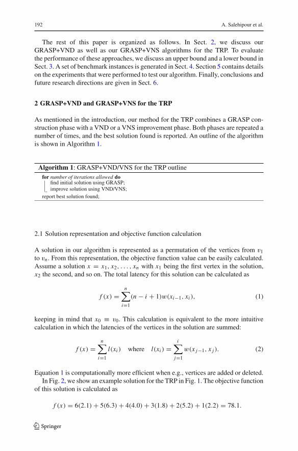
The objective of the TRP is to find an open Hamiltonian circuit, starting from v0,that minimizes the total waiting time. The waiting time of a vertex, also called itslatency, is defined as the time it takes to reach it. The TRP can be seen as a “customer-centric” routing problem, because the objective function minimizes the total waitingtime of all customers (vertices), rather than the travel time of the vehicle the customersis visited with. Besides the obvious applications in customer-centric routing (e.g., adoctor visiting patients, or a repairman visiting machines that require servicing), theTRP has applications in e.g., disk head scheduling. An example traveling repairmanproblem, including a (symmetric) distance matrix, can be found in Fig. 1.

The TRP is very similar to the traveling salesman problem (TSP) and several differ-ent mathematical programming formulations have been proposed [see, e.g., Fischettiet al. 1993; Sarubbi and Luna 2007; Méndez-Díaz et al. 2008]. On a metric space, theTRP is NP-hard (Blum et al. 1994) like the TSP but surprisingly, the TRP is muchharder to solve or approximate. Polynomial time algorithms exist in a number of spe-cial cases, such as paths (Afrati et al. 1986; García et al. 2002) or trees of diameter 3(Blum et al. 1994). A lot of research has gone into developing approximations for theTRP, and the current best approximation ratio is 3.59 (Chaudhuri et al. 2003). In con-trast, the best-known approximation ratio for the metric TSP is 1.5, due to Christofides(1976). As stated by Méndez-Díaz et al. (2008), the TRP is a very hard problem tosolve to proven optimality.

Several exact algorithms for the TRP exist, such as the dynamic programming algo-rithm of Wu (2000) or the much more efficient branch and bound algorithm of Wuet al. (2004). Due to the NP-hardness of the TRP, however, these approaches are unableto solve medium- and large-scale instances. The fastest method of Wu et al. (2004)requires 100 s to solve a problem with approximately 25 vertices, which makes thismethod faster and more powerful than an implementation of CPLEX on a standardformulation.

Fig. 1 Example traveling repairman problem and (symmetric) distance matrix

123

Efficient GRASP+VND and GRASP+VNS 191

Research on the TRP has focused almost exclusively on either approximation algo-rithms or exact methods and this paper presents the first metaheuristic approach forthis problem. However, a limited number of metaheuristics have appeared since thedevelopment of our method. Most notably, the memetic algorithm of Ngeuveu et al.(2010) focuses on a capacitated version of the TRP, called the vehicle routing problemwith cumulative demand.

Our GRASP+VND/VNS approach is a multi-start method in which each iterationconsists of two phases: a greedy randomized construction phase and a variable neigh-borhood descent or variable neighborhood search improvement phase. The approachis tested on a number of instances, both randomly generated ones and instances fromthe TSP Library.1

GRASP (Greedy Randomized Adaptive Search Procedure) was introduced by Feoand Resende (1989, 1995). The basic idea of GRASP is to allow a controlled amountof randomness to overcome the myopic behaviour of a purely greedy heuristic. Thismethod has been applied to a large number of combinatorial optimization problems,including routing problems such as the vehicle routing problem with time windows(Kontoravdis and Bard 1995). Although initial implementations of GRASP com-bined it with simple local search strategies, more recent work combines it with moreadvanced local search approaches.

Among those more advanced local search schemes is variable neighborhood search(VNS) (Mladenovic and Hansen 1997; Hansen and Mladenovic 1999, 2001b), a recentmetaheuristic for combinatorial optimization. VNS is based on the principle of sys-tematically exploring several different neighborhoods, combined with a perturbationmove (called shaking in the VNS literature) to escape from local optima. Despite thefact that it has been developed only recently, variable-neighborhood search has beensuccessfully applied to a wide variety of well-known and lesser-known optimizationproblems (Hansen and Mladenovic 2001a,b). Several researchers have applied someform of VNS to (more or less academic) vehicle routing problems. Two examples areCordone and Wolfler Calvo (2001), in which a VNS algorithm for the vehicle rout-ing problem with time windows is developed, and Crispim and Brandao (2001), whopresent a VNS approach to the vehicle routing problem with backhauls.

Variable neighborhood descent (VND) is essentially a simple variant of VNS, inwhich the shaking phase is omitted. Therefore, contrary to VNS, VND is usually com-pletely deterministic. The combination of GRASP and VND is not new: Ribeiro andVianna (2003), for example, applied it to the phylogeny problem.

It is important however to note that the concept of multiple neighborhood search(i.e., using more than one neighborhood type) is broader than the one proposed invariable neighborhood search and that a large number of non-VNS approaches usedifferent neighborhood types. In the list of best-performing approaches for most vehi-cle routing problems, the idea of multiple neighborhood search is overwhelminglypresent. In their survey article on metaheuristics for the vehicle routing with time win-dows, Bräysy and Gendreau (2005) find that a large majority of tabu search approachesand genetic algorithms use more than one type of neighborhood.

1 http://comopt.ifi.uni-heidelberg.de/software/TSPLIB95/.

123

http://comopt.ifi.uni-heidelberg.de/software/TSPLIB95/


The rest of this paper is organized as follows. In Sect. 2, we discuss ourGRASP+VND as well as our GRASP+VNS algorithms for the TRP. To evaluatethe performance of these approaches, we discuss an upper bound and a lower bound inSect. 3. A set of benchmark instances is generated in Sect. 4. Section 5 contains detailson the experiments that were performed to test our algorithm. Finally, conclusions andfuture research directions are given in Sect. 6.

2 GRASP+VND and GRASP+VNS for the TRP

As mentioned in the introduction, our method for the TRP combines a GRASP con-struction phase with a VND or a VNS improvement phase. Both phases are repeated anumber of times, and the best solution found is reported. An outline of the algorithmis shown in Algorithm 1.

Algorithm 1: GRASP+VND/VNS for the TRP outlinefor number of iterations allowed do

find initial solution using GRASP;improve solution using VND/VNS;

report best solution found;

2.1 Solution representation and objective function calculation

A solution in our algorithm is represented as a permutation of the vertices from v1to vn . From this representation, the objective function value can be easily calculated.Assume a solution x = x1, x2, . . . , xn with x1 being the first vertex in the solution,x2 the second, and so on. The total latency for this solution can be calculated as

f (x) =n∑

i=1

(n − i + 1)w(xi−1, xi ), (1)

keeping in mind that x0 ≡ v0. This calculation is equivalent to the more intuitivecalculation in which the latencies of the vertices in the solution are summed:

f (x) =n∑

i=1

l(xi ) where l(xi ) =i∑

j=1

w(x j−1, x j ). (2)

Equation 1 is computationally more efficient when e.g., vertices are added or deleted.In Fig. 2, we show an example solution for the TRP in Fig. 1. The objective function

of this solution is calculated as

f (x) = 6(2.1)+ 5(6.3)+ 4(4.0)+ 3(1.8)+ 2(5.2)+ 1(2.2) = 78.1.

123


Fig. 2 Example travelingrepairman problem solution

Fig. 3 Proximity matrix for theexample in Fig. 1

Many of the heuristics developed in the following sections require finding theclosest, second-closest, etc. vertex to any given vertex. We therefore pre-process thedistance data and maintain in memory a proximity matrix that contains one row pervertex. The (i + 1)-th row of the matrix contains all vertices (except for vertex vi )in order of proximity to vertex vi . For the example in Fig. 1, the proximity matrix isshown in Fig. 3.

2.2 GRASP

The motivation for using GRASP as a procedure for the TRP is the observation thatthe initial choices of vertices to visit, i.e., the first few vertices in the tour, are moreimportant than later ones. This immediately follows from Eq. 1, from which it is clearthat the i-th distance in the solution is multiplied with a factor n− i + 1. We thereforeexpect a greedy algorithm to perform well, as it attempts to add the shortest possibledistances early on and leaves the longer ones for later. A completely greedy algorithmon the other hand, can be expected to miss some interesting opportunities.

Perhaps the most distinguishing characteristic of GRASP is the way in which it com-bines greediness with randomness in the construction phase. To this end, a restrictedcandidate list (RCL) is built by selecting a subset of all elements in a greedy fashion.Assuming a minimization problem, the RCL contains the elements whose incorpo-ration into the partially built solution would yield the smallest increase in objective

123


function value. From the RCL, an element is then selected at random, after which theRCL is updated to reflect the fact that a new element was added to the solution and isno longer available for selection. Selection of an element and update of the RCL arerepeated until a complete solution has been built. From this solution, a local searchphase starts until a local optimum is found. The size of the RCL, α, is a parameter ofthe GRASP algorithm that controls the balance between greediness and randomness.If α is small, the search is relatively greedy. If α is large, it is relatively random. Inthe extreme cases, setting α = 1 leads to a completely deterministic greedy search,whereas setting α = n entails a completely random search.

The RCL concept can be easily translated to the TRP problem, and efficiently imple-mented using the proximity matrix (see Fig. 3). Starting from vertex v0, the RCL isfilled with the α closest vertices. From this RCL, a random vertex is chosen, say vr .Now, the RCL is filled with the α vertices closest to vr , omitting any elements thathave already been selected. If fewer than α vertices remain, then the size of the RCL isdecreased. A pseudo-code version of the GRASP construction phase of our algorithmfor the TRP is in Algorithm 2.

Algorithm 2: GRASP for the TRPU ← {v1, v2, . . . , vn};vc ← v0;repeat

create RCL with α vertices vi ∈ U closest to vc;select random vertex vr ∈ RCL;U ← U\{vr };vc ← vr ;

until U = ∅ ;

2.3 Variable neighborhood descent and variable neighborhood search

As their names suggest, these metaheuristics systematically explore different neigh-borhood structures. The main idea underlying VNS and VND is that a local optimumrelative to a certain neighborhood structure not necessarily is a local optimum relativeto another neighborhood structure. For this reason, escaping from a local optimumcan be done by changing the neighborhood structure.

Although this is not required, many implementations of VNS and VND use asequence of nested neighborhoods, N1 to Nkmax , in which each neighborhood in thesequence is a superset of its predecessor, i.e., Nk ⊂ Nk+1. The neighborhoods we usedo not possess this property.

Pseudo-code for a basic version of VND is given in Algorithm 3.The difference between VNS and VND is that the former uses a so-called per-

turbation, also called shaking, move. The aim of the perturbation move is to disturbthe current solution in such a way that its structure is partially (but not completely)destroyed. Usually, the perturbation move is executed before the set of neighborhoodsis used to improve the solution. In our algorithm, the perturbation is performed before

123


Algorithm 3: Basic variable neighborhood descentInput: initial solution xinitialise: k ← 1;repeat

local search: x ′ ← arg min Nk (x);if x ′ is better than x then

x ← x ′ and k ← 1 (centre the search around x ′ and search again in the first neighborhood);else

k ← k + 1 (switch to another neighborhood);

until k = kmax ;

each neighborhood, since we found that this yielded better results. The perturbationmove of our VNS algorithm randomly removes a certain fixed percentage (20% in ourexperiments) of the customers in the current solution and inserts them in a different,random location. Pseudo-code for the variant of VNS that is used in our algorithm isgiven in Algorithm 4. Our VNS deviates from the “standard” VNS in that it does notre-center around the best-known solution after the perturbation phase.

Algorithm 4: Basic variable neighborhood searchInput: initial solution xinitialise: k ← 1;repeat

perturb: x ′ ← x ;local search: x ′′ ← arg min Nk (x ′);if x ′′ is better than x then

x ← x ′′ and k ← 1 (centre the search around x ′′ and search again in the first neighborhood);else

k ← k + 1 (switch to another neighborhood);

until k = kmax ;

Usually, VNS/VND algorithms examine all neighborhoods in a certain order, fromsmall to large. The reason is that small neighborhoods contain fewer solutions andcan hence be searched in less time than large neighborhoods. Larger neighborhoodsare only examined when all smaller neighborhoods have been depleted, i.e., when thecurrent solution is a local optimum relative to all smaller neighborhoods. The VNDstops when the solution is a local optimum of all neighborhoods. Another option isto explore the neighborhoods in the order of their effectiveness with respect to theproblem at hand, which can be established by means of a small pilot study.

2.3.1 Neighborhoods

Our search uses five neighborhood structures: swap, swap-adjacent, 2-opt, Or-opt, andremove–insert. In a pilot study, we found that the performance of the algorithm is rela-tively insensitive to the order in which the neighborhoods are used. The neighborhoods

123


are therefore explored in a specific order, from “small” to “large” as it is common inVNS algorithms, i.e., swap-adjacent, remove-insert, swap, 2-opt and Or-opt.

The swap heuristic attempts to swap the positions of each pair of vertices in thesolution (see Fig. 4). Searching the entire neighborhood of a solution with this heuris-tic requires quadratic time in the problem size (O(n2)). Using Eq. 1, examining theeffect of a swap of vertices xi and x j in solution x on the objective function value canbe easily done by subtracting the weight of the removed edges and adding that of thenew edges in the solution.

The swap-adjacent heuristic, as its name suggests, attempts to swap each pair ofadjacent vertices in the solution x . This heuristic examines a subset of the movesexplored in the swap heuristic and has a linear complexity (O(n)).

The 2-opt heuristic (see Fig. 5) removes each pair of edges from the solution andreconnects the vertices. Updating the objective function is more complicated for 2-opt,since the middle part of the solution (that was “cut out”) is reversed. This heuristicrequires O(n2) time to examine the entire neighborhood of a solution.

The Or-opt heuristic (see Fig. 6) removes each triplet of edges from the solutionand reconnects the vertices in such a way that the orientation of the solution parts ispreserved. The time complexity of this heuristic is cubic (O(n3)).

The remove–insert heuristic examines each vertex xi in the solution and placesthe vertex furthest away from xi at the end of the solution. This heuristic has linearcomplexity like the swap-adjacent heuristic.

Fig. 4 Swap

Fig. 5 2-opt

123


Fig. 6 Or-opt

2.3.2 Neighborhood reduction

We made several attempts to decrease the size of the neighborhoods to examine dur-ing the local search phase. All neighborhood reduction schemes are carefully testedin Sect. 5.

For the swap, 2-opt and Or-opt moves the neighborhood size is reduced by fix-ing a random vertex and then attempting only the moves that involve this vertex.We call this strategy “Fix” and compare it to the “NoFix” strategy in which theentire neighborhood is searched without first fixing a random vertex. This neigh-borhood reduction scheme decreases the size of the neighborhood by a factorO(n).

A second neighborhood reduction scheme is based on the observation thatin a reasonably good solution, most improving moves will involve vertices thatappear in relative proximity in this solution. For example, in a good solution itis unlikely that a swap will yield a better solution if it exchanges a vertex thatappears close to the depot with one that appears far from the depot. We thereforeintroduce a proximity factor β to determine the maximum distance between ver-tices that may be involved in a move. The factor β has a slightly different influ-ence, depending on the move. For a swap move, the second vertex may be onlyβ positions further in the solution than the first one. For a 2-opt move, the headof the second chosen arc may only be β positions further in the solution thanthe head of the first chosen arc. For an Or-opt move, the heads of both the sec-ond and third chosen arcs may be only β positions away from the head of thefirst arc. For the swap-adjacent and remove–insert heuristics, we did not use thisstrategy.

3 Bounds for the TRP

We compare the outcome of our algorithm to an upper and a lower bound, discussedin this section. Due to the specific properties of the TRP, deriving good bounds isdifficult. As explained in Blum et al. (1994), the TRP cannot be simply considereda variant of the TSP. The gap between the upper and the lower bounds are thereforerelatively large.

123


3.1 Upper bound

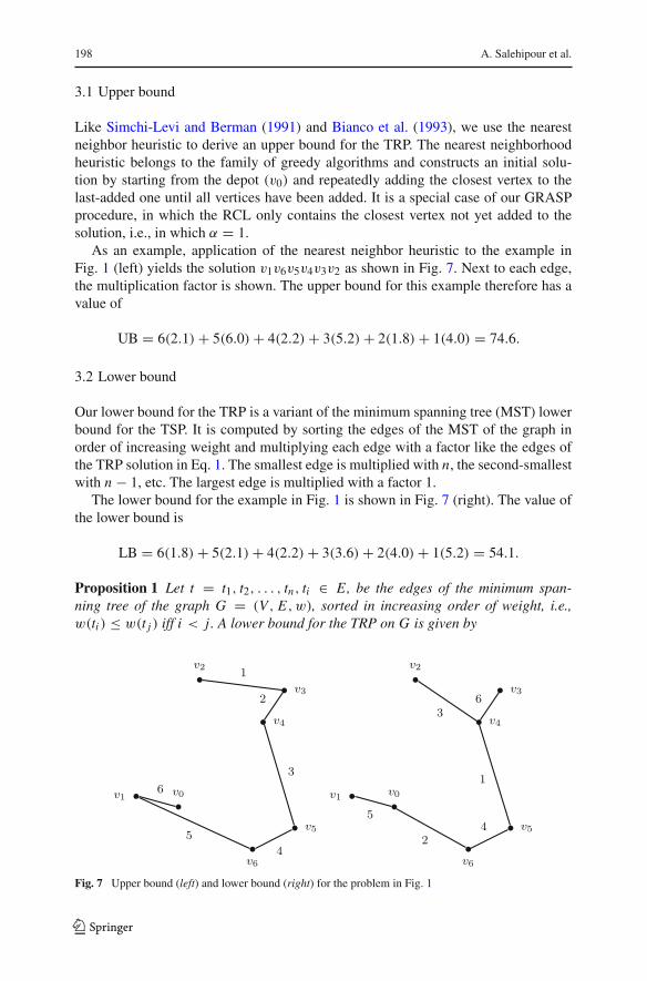
Like Simchi-Levi and Berman (1991) and Bianco et al. (1993), we use the nearestneighbor heuristic to derive an upper bound for the TRP. The nearest neighborhoodheuristic belongs to the family of greedy algorithms and constructs an initial solu-tion by starting from the depot (v0) and repeatedly adding the closest vertex to thelast-added one until all vertices have been added. It is a special case of our GRASPprocedure, in which the RCL only contains the closest vertex not yet added to thesolution, i.e., in which α = 1.

As an example, application of the nearest neighbor heuristic to the example inFig. 1 (left) yields the solution v1v6v5v4v3v2 as shown in Fig. 7. Next to each edge,the multiplication factor is shown. The upper bound for this example therefore has avalue of

UB = 6(2.1)+ 5(6.0)+ 4(2.2)+ 3(5.2)+ 2(1.8)+ 1(4.0) = 74.6.

3.2 Lower bound

Our lower bound for the TRP is a variant of the minimum spanning tree (MST) lowerbound for the TSP. It is computed by sorting the edges of the MST of the graph inorder of increasing weight and multiplying each edge with a factor like the edges ofthe TRP solution in Eq. 1. The smallest edge is multiplied with n, the second-smallestwith n − 1, etc. The largest edge is multiplied with a factor 1.

The lower bound for the example in Fig. 1 is shown in Fig. 7 (right). The value ofthe lower bound is

LB = 6(1.8)+ 5(2.1)+ 4(2.2)+ 3(3.6)+ 2(4.0)+ 1(5.2) = 54.1.

Proposition 1 Let t = t1, t2, . . . , tn, ti ∈ E, be the edges of the minimum span-ning tree of the graph G = (V, E, w), sorted in increasing order of weight, i.e.,w(ti ) ≤ w(t j ) iff i < j . A lower bound for the TRP on G is given by

Fig. 7 Upper bound (left) and lower bound (right) for the problem in Fig. 1

123


LB =n∑

i=1

(n − i + 1)w(ti ), (3)

where w(ti ) is the weight of edge ti .

Proof Assume that the optimal traveling repairman solution of G = (V, E, w) isgiven by r = r1, r2, . . . , rn, ri ∈ E , with the edges in order of appearance in thesolution. The objective function value of r is f (r) =∑n

i=1(n − i + 1)w(ri ).Since t is a minimum spanning tree, the edges t1, t2, . . . , ti form the set of the i

smallest edges of the graph that do not form a cycle. It holds that the sum of the weightsof the i smallest edges that do not form a cycle, is smaller than the sum of the weightsof any other i edges that do not form a cycle. Since the first i edges in the travelingrepairman solution also do not form a cycle, it follows that

i∑

j=1

w(t j ) ≤i∑

j=1

w(r j ).

Summing over i , we get that

n∑

i=1

i∑

j=1

w(t j ) ≤n∑

i=1

i∑

j=1

w(r j ),

which simplifies to

n∑

i=1

(n − i + 1)w(ti ) ≤n∑

i=1

(n − i + 1)w(ri ).

4 Benchmark instance set generation

To the best of our knowledge, no standard set of medium- and large-scale benchmarkinstances for the TRP exists. We therefore test our algorithm on (1) an extensive setof 140 self-generated symmetric instances of seven different problem sizes rangingfrom 10 to 1000 vertices (10, 20, 50, 100, 200, 500, 1000) and (2) a selection of teninstances from the TSP Library.

To create our own set of 140 test instances, we have generated 20 random instancesfor each problem size. For each instance, vertex coordinates have been generated froma uniform distribution between 0 and 100 (or between 0 and 500 for the instances ofsize 500 and 1000). All distances are Euclidean, rounded down to the nearest integer.The instances are available from the authors upon request (Table. 1).

123


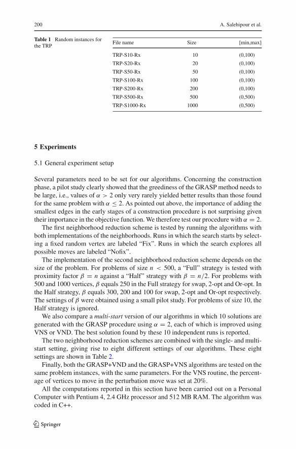
Table 1 Random instances forthe TRP

File name Size [min,max]

TRP-S10-Rx 10 (0,100)

TRP-S20-Rx 20 (0,100)

TRP-S50-Rx 50 (0,100)

TRP-S100-Rx 100 (0,100)

TRP-S200-Rx 200 (0,100)

TRP-S500-Rx 500 (0,500)

TRP-S1000-Rx 1000 (0,500)

5 Experiments

5.1 General experiment setup

Several parameters need to be set for our algorithms. Concerning the constructionphase, a pilot study clearly showed that the greediness of the GRASP method needs tobe large, i.e., values of α > 2 only very rarely yielded better results than those foundfor the same problem with α ≤ 2. As pointed out above, the importance of adding thesmallest edges in the early stages of a construction procedure is not surprising giventheir importance in the objective function. We therefore test our procedure with α = 2.

The first neighborhood reduction scheme is tested by running the algorithms withboth implementations of the neighborhoods. Runs in which the search starts by select-ing a fixed random vertex are labeled “Fix”. Runs in which the search explores allpossible moves are labeled “Nofix”.

The implementation of the second neighborhood reduction scheme depends on thesize of the problem. For problems of size n < 500, a “Full” strategy is tested withproximity factor β = n against a “Half” strategy with β = n/2. For problems with500 and 1000 vertices, β equals 250 in the Full strategy for swap, 2-opt and Or-opt. Inthe Half strategy, β equals 300, 200 and 100 for swap, 2-opt and Or-opt respectively.The settings of β were obtained using a small pilot study. For problems of size 10, theHalf strategy is ignored.

We also compare a multi-start version of our algorithms in which 10 solutions aregenerated with the GRASP procedure using α = 2, each of which is improved usingVNS or VND. The best solution found by these 10 independent runs is reported.

The two neighborhood reduction schemes are combined with the single- and multi-start setting, giving rise to eight different settings of our algorithms. These eightsettings are shown in Table 2.

Finally, both the GRASP+VND and the GRASP+VNS algorithms are tested on thesame problem instances, with the same parameters. For the VNS routine, the percent-age of vertices to move in the perturbation move was set at 20%.

All the computations reported in this section have been carried out on a PersonalComputer with Pentium 4, 2.4 GHz processor and 512 MB RAM. The algorithm wascoded in C++.

123


Table 2 Experiment settingsfor GRASP+VNS andGRASP+VND

Restarts Neighborhood Proximity Experimentimplementation rule number

Single-start Nofix Full 1

Half 2

Fix Full 3

Half 4

Multi-start Nofix Full 5

Half 6

Fix Full 7

Half 8

Table 3 Comparison of theGRASP+VNS metaheuristicwith CPLEX on instances with10 customers

Best result in bold

GRASP+VNS CPLEX

Obj. T Obj. T

R1 1303 0.00 1303 81

R2 1517 0.00 1517 61

R3 1233 0.00 1233 65

R4 1386 0.00 1386 90

R5 978 0.00 978 61

R6 1477 0.00 1477 217

R7 1163 0.00 1163 146

R8 1234 0.00 1234 222

R9 1402 0.00 1402 164

R10 1388 0.00 1388 261

R11 1405 0.00 1405 122

R12 1150 0.00 1150 125

R13 1531 0.00 1531 570

R14 1219 0.00 1219 122

R15 1087 0.00 1087 127

R16 1264 0.00 1264 489

R17 1058 0.00 1058 30

R18 1083 0.00 1083 34

R19 1394 0.00 1394 228

R20 951 0.00 951 25

Average 0.00 162

5.2 Comparison with CPLEX on small instances

A comparison of our GRASP+VNS with CPLEX on small instances is reported inTables 3 and 4. In each of these cases, we ran the best two configurations of ourmetaheuristic (multi-start GRASP+VNS with Fix neighborhood implementation andHalf or Full proximity rule) on all the instances and report the best of the two results.Table 3 displays the results of both methods on instances with 10 customers. Column

123


Table 4 Comparison of the GRASP+VNS metaheuristic with CPLEX on instances with 20 customers

GRASP+VNS CPLEX (1h) CPLEX (24h)

Obj. T Obj. Gap (%) � (%) Obj. Gap (%) � (%)

R1 3175 <0.02 3224 41.55 1.52 3175 22.17 0.00

R2 3248 <0.02 3440 57.30 5.58 3248 23.56 0.00

R3 3570 <0.02 4141 57.48 13.79 3570 31.09 0.00

R4 2983 <0.02 3317 48.51 10.07 3065 17.81 2.68

R5 3248 <0.02 3732 59.28 12.97 3365 39.22 3.48

R6 3328 <0.02 3426 55.96 2.86 3328 33.11 0.00

R7 2809 <0.02 3286 61.23 14.52 2809 41.07 0.00

R8 3461 <0.02 3605 54.37 3.99 3461 22.14 0.00

R9 3475 <0.02 4285 58.87 18.90 3392 19.33 −2.45

R10 3359 <0.02 3707 56.31 9.39 3359 21.25 0.00

R11 2916 <0.02 3074 49.60 5.14 2916 26.64 0.00

R12 3314 <0.02 3468 47.11 4.44 3314 21.11 0.00

R13 3412 <0.02 3427 56.58 0.44 3412 27.78 0.00

R14 3297 <0.02 3458 56.59 4.66 3297 23.45 0.00

R15 2862 <0.02 2881 39.88 0.66 2862 19.12 0.00

R16 3433 <0.02 3909 57.01 12.18 3433 23.22 0.00

R17 2924 <0.02 2977 57.47 1.78 2924 21.15 0.00

R18 3168 <0.02 3467 61.08 8.62 3150 31.03 −0.57

R19 3299 <0.02 3503 42.35 5.82 3299 19.87 0.00

R20 2796 <0.02 2842 42.18 1.62 2796 15.11 0.00

Average <0.02 53.04 6.95 25.06 0.16

Best result in bold

T shows the computing time in seconds. As can be seen, CPLEX finds the optimalsolutions to all 20 random instances in an average time of 162 seconds. Our methodfinds all optimal solutions as well, albeit in a much smaller amount of time (less than0.005 seconds) in each case.

In Table 4, results for instances with 20 customers are shown. In this case, CPLEXis not able to prove the optimality of the solutions it finds in 1 day of computing time:the average optimality gap is 53% after 1 hour and 25% after 24 hours of computation.In 16 out of 20 instances our GRASP+VNS metaheuristic finds the same solution asCPLEX (in less than 0.02 seconds for each case), and in 2 cases (R4 and R5) it findsa better solution. In only two cases is CPLEX able to find a better solution after 24hours of calculation. Gaps for larger instances were considered too large to providea meaningful benchmark. These findings are in line with those of Méndez-Díaz et al.(2008), who conclude that the TRP is a very hard problem to solve to optimality.

5.3 Results on larger instances

The full results of our GRASP+VND algorithm on the randomly generated data setsare reported in Table 5, while those of the GRASP+VNS algorithm are in Table 6.

123


Table 5 Results of the GRASP+VND

n Single-start

1 (Nofix-Full) 2 (Nofix-Half)

UB% LB% T Tbest UB% LB% T Tbest

10 2.14 33.48 0.00 0.00 – – – –

20 8.19 42.43 0.00 0.00 6.89 44.75 0.00 0.00

50 6.85 50.07 0.27 0.21 6.70 50.21 0.03 0.00

100 10.24 45.53 9.73 8.91 9.99 45.97 1.21 1.11

200 10.69 43.37 356.73 319.45 10.20 44.18 39.81 35.02

500 10.70 46.49 7192.94 7002.09 10.49 46.84 635.96 598.00

1000 – – – – 11.32 46.40 3378.28 3013.29

n Single-start

3 (Fix-Full) 4 (Fix-Half)


10 1.96 33.71 0.00 0.00 – – – –

20 7.51 43.45 0.00 0.00 6.51 45.19 0.00 0.00

50 5.69 51.95 0.01 0.00 5.24 52.64 0.00 0.00

100 8.55 48.33 0.32 0.11 8.56 48.30 0.07 0.04

200 8.61 46.77 6.30 4.98 8.54 46.88 1.25 1.09

500 9.19 48.97 134.83 112.14 9.18 49.00 18.86 13.30

1000 9.31 49.72 837.26 787.63 9.22 49.88 112.99 106.37

n Multi-start



10 2.44 33.04 0.00 0.00 – – – –

20 9.86 39.63 0.04 0.00 9.80 39.80 0.00 0.00

50 9.67 45.41 3.21 3.01 9.48 45.71 0.43 0.31

100 11.56 43.40 101.27 91.12 11.21 43.93 12.55 10.79

200 11.33 42.32 3741.05 3225.03 11.44 42.14 444.43 397.42

500 8.11 50.73 91470.78 86431.76 11.47 45.22 6335.79 6115.69

1000 – – – – 8.18 51.57 9114.75 8912.23

n Multi-start



10 2.44 33.04 0.00 0.00 – – – –

20 9.41 40.34 0.01 0.00 9.70 39.82 0.00 0.00

50 8.29 47.59 0.19 0.10 7.83 48.40 0.04 0.00

123


Table 5 continued

n Multi-start



100 8.43 48.43 3.54 3.01 8.80 47.82 0.80 0.62

200 7.75 48.07 78.25 61.22 7.76 48.05 16.56 13.71

500 8.11 50.73 1534.90 1418.73 8.07 50.81 239.44 216.41

1000 – – – – 8.09 51.73 1431.16 1297.09

The results of the GRASP+VND algorithm on the TSP Library instances can be foundin Tables 7, 8 and 9. In all tables, the column labeled UB% shows the improvementof the objective function over the upper bound obtained with the nearest neighborheuristic. The column labeled LB% shows the gap to the lower bound, obtained usingthe minimum spanning tree with edge multiplicator. In the column labeled T , thecomputation time until the algorithm stops (in seconds) is shown. Column Tbest inTables 5 and 6 contains the computation time (in seconds) at which the best solutionwas reached by the GRASP+VND and GRASP+VNS algorithms respectively.

From Tables 5 to 6 we can draw some conclusions about the working of our algo-rithm. Unsurprisingly, the multi-start version of our algorithm (algorithm settings 5to 8) requires a much larger computation time than the single-start version (settings 1to 4). However, the quality improvement obtained by this method is relatively small.The perturbations in the GRASP+VNS algorithm (Table 6) seem to help marginally, asthe solutions obtained by this algorithm are usually slightly better. This may indicatethat the GRASP multi-start is not able to provide enough diversification, and that theperturbation move is useful.

Both neighborhood reduction strategies seem to work well. The neighborhoodimplementation with fixed random vertex (Fix, settings 3, 4, 7, and 8) uses signif-icantly less computing time, combined with a rather small loss of solution quality. TheHalf neighborhood reduction strategy (settings 2, 4, 6, and 8) yields a much faster solu-tion method, at the cost of some loss in objective function quality. Both neighborhoodreduction strategies prove useful for the largest instances (500 and 1000 vertices), forwhich full neighborhood search (Full and NoFix) was too time consuming.

Tables 7, 8 and 9 show the results of the algorithm on a selected set of TSPlibinstances. Conclusions on the working of our algorithm that can be drawn from theseexperiments are in line with the ones on randomly generated instances. Table 9 shows—unsurprisingly—that the optimal TSP-solution is generally not a good solution to theTRP on the same instance. On average, the best solution found by our algorithm isalmost 17% better than the optimal TSP-solution.

6 Conclusions and future research

In this paper, we have presented the first metaheuristics for the traveling repairmanproblem. These metaheuristics consists of a GRASP construction phase and a variable

123


Table 6 Results of the GRASP+VNS

n Single-start



10 2.14 33.48 0.00 0.00 – – – –

20 8.19 42.43 0.00 0.00 6.89 44.75 0.00 0.00

50 6.87 50.05 0.29 0.18 6.69 50.21 0.03 0.00

100 10.54 45.04 11.99 8.32 10.33 45.42 1.68 1.11

200 10.82 43.16 378.68 311.02 10.18 44.23 46.11 3.75

500 10.93 46.12 7373.09 6951.22 10.93 46.11 693.16 604.89

1000 – – – – 11.57 45.99 4103.28 3876.51

n Single-start


UB% LB% T Tbest UB% LB% T Tbest10 1.96 33.71 0.00 0.00 – – – –

20 7.51 43.45 0.00 0.00 6.51 45.19 0.00 0.00

50 5.69 51.94 0.02 0.00 5.27 52.60 0.00 0.00

100 9.04 47.53 0.36 0.21 8.73 48.02 0.09 0.06

200 13.40 38.87 7.57 5.99 9.05 46.03 1.51 1.19

500 9.57 48.35 150.33 111.10 9.36 48.71 20.71 16.77

1000 9.79 48.94 1404.56 1163.49 9.80 48.92 137.39 119.29

n Multi-start



20 9.86 39.63 0.04 0.00 14.25 33.06 0.00 0.00

50 9.74 45.30 3.54 3.14 9.67 45.39 1.91 1.77

100 11.66 43.26 103.92 89.12 11.35 43.73 12.95 10.88

200 16.21 34.96 3995.00 3752.26 16.24 34.92 476.41 409.33

500 9.71 48.14 10381.36 9065.10 11.84 44.62 6918.79 6223.00

1000 – – – – – – – –

n Multi-start

7(Fix-Full) 8(Fix-Half)


20 9.41 40.34 0.01 0.00 14.15 33.08 0.00 0.00

50 8.54 47.20 0.58 0.08 8.55 47.21 0.07 0.03

100 11.00 44.28 3.97 2.95 9.79 46.15 0.94 0.69

123


Table 6 continued

n Multi-start

7(Fix-Full) 8(Fix-Half)


200 13.86 38.77 82.37 68.03 13.02 40.08 18.70 13.97

500 8.87 49.50 1825.40 1524.09 8.20 50.60 284.00 195.51

1000 13.76 42.35 11031.62 9311.21 12.91 43.77 1906.01 1599.57

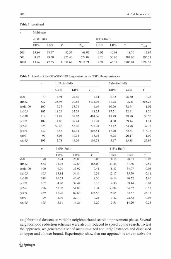
Table 7 Results of the GRASP+VND Single-start on the TSP Library instances

n 1 (Nofix-Full) 2 (Nofix-Half)

UB% LB% T UB% LB% T

st70 70 4.94 27.66 2.14 6.62 26.50 0.23

att532 532 35.98 30.56 5134.36 31.98 32.6 555.27

kroD100 100 9.37 33.74 4.69 10.70 32.94 1.02

lin105 105 18.29 32.29 11.25 17.21 32.91 1.20

lin318 318 17.89 39.62 401.06 19.49 38.80 50.70

pr107 107 4.80 39.44 15.28 4.80 39.44 1.14

pr226 226 52.46 55.06 228.78 53.42 54.78 37.78

pr439 439 16.53 82.44 508.84 17.20 82.34 613.73

rat99 99 8.04 19.38 13.98 6.98 20.17 1.00

rat195 195 3.78 14.04 104.38 3.97 13.88 27.97

n 3 (Fix-Full) 4 (Fix-Half)

UB% LB% T UB% LB% Tst70 70 3.24 28.83 0.08 8.18 28.83 0.02

att532 532 31.93 32.63 165.00 33.44 31.86 19.59

kroD100 100 9.01 33.97 0.41 8.83 34.07 0.08

lin105 105 13.84 34.84 0.34 12.17 35.79 0.11

lin318 318 16.25 40.46 8.30 16.14 40.52 2.80

pr107 107 4.80 39.44 0.16 4.80 39.44 0.03

pr226 226 53.07 54.88 5.34 53.94 54.62 0.53

pr439 439 15.26 82.63 125.56 15.65 82.57 23.33

rat99 99 4.39 22.10 0.24 3.42 22.82 0.03

rat195 195 3.51 14.26 7.20 3.51 14.26 0.28

neighborhood descent or variable neighbourhood search improvement phase. Severalneighborhood reduction schemes were also introduced to speed up the search. To testthe approach, we generated a set of medium-sized and large instances and discussedan upper and a lower bound. Experiments show that our approach is able to solve the

123


Table 8 Results of the GRASP+VND Multi-start on the TSPlib instances

n 5 (Nofix-Full) 6 (Nofix-Half)

UB% LB% T UB% LB% T

st70 70 5.26 27.44 22.24 6.62 26.50 2.23

att532 532 52.51 22.11 65121.06 43.29 26.82 5005.32

kroD100 100 11.29 32.59 54.69 11.16 32.66 11.02

lin105 105 19.04 31.85 101.27 17.41 32.79 12.23

lin318 318 22.92 37.04 3951.02 19.70 38.69 455.60

pr107 107 21.52 29.78 225.32 8.63 37.23 3.33

pr226 226 54.00 54.60 2328.71 53.42 54.78 239.56

pr439 439 23.13 81.45 4563.44 20.44 81.85 5614.74

rat99 99 9.77 18.09 195.31 6.98 20.17 9.00

rat195 195 4.56 13.39 884.78 4.46 13.48 311.97

n 7 (Fix-Full) 8 (Fix-Half)

UB% LB% T UB% LB% Tst70 70 7.45 25.93 1.10 6.28 30.07 1.11

att532 532 42.41 27.27 1065.09 27.89 34.69 317.09

kroD100 100 9.22 33.84 3.13 9.22 33.84 1.12

lin105 105 14.88 34.24 3.09 13.56 34.99 1.44

lin318 318 17.03 40.06 79.79 11.45 42.92 12.24

pr107 107 8.18 37.49 1.89 2.82 40.58 0.10

pr226 226 53.07 54.88 53.22 53.49 54.75 3.23

pr439 439 14.66 82.72 1256.31 15.20 82.64 196.22

rat99 99 6.01 20.89 2.95 6.01 20.89 1.02

rat195 195 1.99 15.52 55.46 2.93 14.74 1.05

Table 9 Comparison of the best-found TRP-solution with the optimal TSP-solution using theTRP-objective function

Problem Optimal TSP Best TRP Difference % Difference

st70 22865 19553 3312 16.94

att532 24186404 18448435 5737969 31.10

kroD100 1072593 976830 95763 9.80

lin105 904993 585823 319170 54.48

lin318 7238644 5876537 1362107 23.18

pr107 2040746 1983475 57271 2.89

pr226 8284243 7226554 1057689 14.64

pr439 19305544 18567170 738374 3.98

rat99 60415 56994 3421 6.00

rat195 226194 213371 12823 6.01

Average 16.90

123


generated instances, as well as a set of instances drawn from the TSP library, in areasonable amount of time.

In the future, we intend to extend our algorithm by including more neighborhoodsand carefully studying the effectiveness of each neighborhood on the TRP. We alsointend to apply our algorithm to other customer-centric routing problems, involvingmore than one vehicle. Increasing the efficiency of our algorithm even more, to alloweven larger problems to be solved, is another future research topic. Finally, the inte-gration of exact methods for the TRP might lead to even better performing algorithmsand is something that we plan to investigate.

While this paper was in the final stage of the review process, follow-up work waspublished by Ngeuveu et al. (2010). Although their focus is on the capacitated TRP,they suggest various procedures that would speed up the search for optimal solutionsfor the uncapacitated TRP and that, in general, lead to better solutions. Incorporationof such procedures in our GRASP+VNS/VND method is also left for future research.

Open Access This article is distributed under the terms of the Creative Commons Attribution Noncom-mercial License which permits any noncommercial use, distribution, and reproduction in any medium,provided the original author(s) and source are credited.

References

Afrati F, Cosmadakis S, Papadimitriou CH, Papageorgiou G, Papakostantinou N (1986) The complexity ofthe traveling repairman problem. Theor Inform Appl 20:79–87

Bianco L, Mingozzi A, Ricciardelli S (1993) The travelling salesman problem with cumulative costs.Networks 23(2):81–91

Blum A, Chalasani P, Coppersmith D, Pulleyblank B, Raghavan P, Sudan M (1994) The minimum latencyproblem. In: Proceedings of the twenty-sixth annual symposium on theory of computing (STOC),pp 163–171

Bräysy O, Gendreau M (2005) Vehicle routing problem with time windows, part II: metaheuristics. Trans-port Sci 39:119–139

Chaudhuri K, Godfrey B, Rao S, Talwar K (2003) Paths, trees, and minimum latency tours. In: Proceedingsof 44th symposium on foundations of computer science (FOCS), pp 36–45

Christofides N (1976) Worst-case analysis of a new heuristic for the travelling salesman problem.Technical Report 388, Graduate School of Industrial Administration, Carnegie-Mellon University,Pittsburgh, PA

Cordone R, Wolfler Calvo R (2001) A heuristic for the vehicle routing problem with time windows.J Heuristics 7:107–129

Crispim J, Brandao J (2001) Reactive tabu search and variable neighborhood descent applied to the vehi-cle routing problem with backhauls. In: MIC 2001—Proceedings of the metaheuristics internationalconference, Porto, pp 631–636

Feo TA, Resende MGC (1989) A probabilistic heuristic for a computationally difficult set covering problem.Oper Res Lett 8:67–71

Feo TA, Resende MGC (1995) Greedy randomized adaptive search procedures. J Global Optim 6:109–133Fischetti M, Laporte G, Martello S (1993) The delivery man problem and cumulative matroids. Oper Res

41(6):1055–1064García A, Jodrá P, Tejel J (2002) A note on the traveling repairman problem. Networks 40(1):27–31Hansen P, Mladenovic N (1999) An introduction to variable neighborhood search. In: Voss S, Martello S,

Osman I, Roucairol C (eds) Metaheuristics: advances and trends in local search paradigms for opti-mization. Kluwer, Boston pp 433–458

Hansen P, Mladenovic N (2001a) Industrial applications of the variable neighbourhood search metaheuristic.In: Decisions and control in management science. Kluwer, Boston, pp 261–274

123


Hansen P, Mladenovic N (2001b) Variable neighbourhood search: principles and applications. Eur J OperRes 130:449–467

Kontoravdis GA, Bard JF (1995) A GRASP for the vehicle routing problem with time windows. INFORMSJ Comput 7:10–23

Mladenovic N, Hansen P (1997) Variable neighbourhood search. Comput Oper Res 24:1097–1100Méndez-Díaz I, Zabala P, Lucena A (2008) A new formulation for the traveling deliveryman problem.

Discrete Appl Math 156(17):3223–3237Ngeuveu SU, Prins C, Wolfler Calvo R (2010) An effective memetic algorithm for the cumulative capaci-

tated vehicle routing problem. Comput OR 37(11):1877–1885Ribeiro CC, Vianna DS (2003) A GRASP/VND heuristic for the phylogeny problem using a new neigh-

borhood structure. Technical report, Department of Computer Science, Catholic U. of Rio de Janeiro,Rio de Janeiro, Brazil

Sarubbi J, Luna H (2007) A new flow formulation for the minimum latency problem. In: Internationalnetwork optimization conference (INOC), Spa, Belgium

Simchi-Levi D, Berman O (1991) Minimizing the total flow time of n jobs on a network. IIE Trans23(3):236–244

Wu BY (2000) Polynomial time algorithms for some minimum latency problems. Inform Process Lett75:225–229

Wu BY, Huang Z-N, Zhan F-J (2004) Exact algorithms for the minimum latency problem. Inform ProcessLett 92:303–309

123

efﬁcient grasp+vnd and grasp+vns metaheuristics for the ... · efﬁcient grasp+vnd and grasp+vns...

Documents