learning to discover sparse graphical...

Learning to Discover Sparse Graphical Models

Eugene Belilovsky 1 2 3 Kyle Kastner 4 Gael Varoquaux 2 Matthew B. Blaschko 1

AbstractWe consider structure discovery of undirectedgraphical models from observational data. Infer-ring likely structures from few examples is a com-plex task often requiring the formulation of priorsand sophisticated inference procedures. Popularmethods rely on estimating a penalized maximumlikelihood of the precision matrix. However, inthese approaches structure recovery is an indirectconsequence of the data-fit term, the penalty canbe difficult to adapt for domain-specific knowl-edge, and the inference is computationally de-manding. By contrast, it may be easier to gener-ate training samples of data that arise from graphswith the desired structure properties. We proposehere to leverage this latter source of informationas training data to learn a function, parametrizedby a neural network, that maps empirical co-variance matrices to estimated graph structures.Learning this function brings two benefits: it im-plicitly models the desired structure or sparsityproperties to form suitable priors, and it can betailored to the specific problem of edge structurediscovery, rather than maximizing data likelihood.Applying this framework, we find our learnablegraph-discovery method trained on synthetic datageneralizes well: identifying relevant edges inboth synthetic and real data, completely unknownat training time. We find that on genetics, brainimaging, and simulation data we obtain perfor-mance generally superior to analytical methods.

IntroductionProbabilistic graphical models provide a powerful frame-work to describe the dependencies between a set of vari-ables. Many applications infer the structure of a probabilis-tic graphical model from data to elucidate the relationships

1KU Leuven 2INRIA 3University of Paris-Saclay 4Universityof Montreal. Correspondence to: Eugene Belilovsky <[email protected]>.

Proceedings of the 34 th International Conference on MachineLearning, Sydney, Australia, PMLR 70, 2017. Copyright 2017 bythe author(s).

between variables. These relationships are often representedby an undirected graphical model also known as a MarkovRandom Field (MRF). We focus on a common MRF model,Gaussian graphical models (GGMs). GGMs are used instructure-discovery settings for rich data such as neuroimag-ing, genetics, or finance (Friedman et al., 2008; Ryali et al,2012; Mohan et al., 2012; Belilovsky et al., 2016). Althoughmultivariate Gaussian distributions are well-behaved, deter-mining likely structures from few examples is a difficult taskwhen the data is high dimensional. It requires strong priors,typically a sparsity assumption, or other restrictions on thestructure of the graph, which now make the distributiondifficult to express analytically and use.

A standard approach to estimating structure with GGMs inhigh dimensions is based on the classic result that the zerosof a precision matrix correspond to zero partial correlation,a necessary and sufficient condition for conditional indepen-dence (Lauritzen, 1996). Assuming only a few conditionaldependencies corresponds to a sparsity constraint on theentries of the precision matrix, leading to a combinatorialproblem. Many popular approaches to learning GGMs canbe seen as leveraging the `1-norm to create convex surro-gates to this problem. Meinshausen & Bühlmann (2006)use nodewise `1 penalized regressions, while other estima-tors penalize the precision matrix directly (Cai et al., 2011;Friedman et al., 2008; Ravikumar et al., 2011), the mostpopular being the graphical lasso

fgl(Σ) = arg minΘ�0− log |Θ|+Tr (ΣΘ) + λ‖Θ‖1 (1)

which can be seen as a penalized maximum-likelihood esti-mator. Here Θ and Σ are the precision and sample covari-ance matrices, respectively. A large variety of alternativepenalties extend the priors of the graphical lasso (Dana-her et al., 2014; Ryali et al, 2012; Varoquaux et al., 2010).However, this strategy faces several challenges. Construct-ing novel surrogates for structured-sparsity assumptions onMRF structures is difficult, as priors need to be formulatedand incorporated into a penalized maximum likelihood ob-jective which then calls for the development of an efficientoptimization algorithm, often within a separate research ef-fort. Furthermore, model selection in a penalized maximumlikelihood setting is difficult as regularization parametersare often unintuitive.

We propose to learn the estimator. Rather than manually de-


signing a specific graph-estimation procedure, we frame thisestimator-engineering problem as a learning problem, se-lecting a function from a large flexible function class by riskminimization. This allows us to construct a loss functionthat explicitly aims to recover the edge structure. Indeed,sampling from a distribution of graphs and empirical covari-ances with desired properties is often possible, even whenthis distribution is not analytically tractable. As such wecan perform empirical risk minimization to select an appro-priate function for edge estimation. Such a framework givesmore control on the assumed level of sparsity (as opposedto graph lasso) and can impose structure on the sampling toshape the expected distribution, while optimizing a desiredperformance metric.

For particular cases we show that the problem of interestcan be solved with a polynomial function, which is learn-able with a neural network (Andoni et al., 2014). Motivatedby this fact, as well as theoretical and empricial resultson learning smooth functions approximating solutions tocombinatorial problems (Cohen et al., 2016; Vinyals et al.,2015), we propose to use a particular convolutional neuralnetwork as the function class. We train it by sampling smalldatasets, generated from graphs with the prescribed proper-ties, with a primary focus on sparse graphical models. Weestimate from this data small-sample covariance matrices(n < p), where n is the number of samples and p is thedimensionality of the data. Then we use them as trainingdata for the neural network (Figure 2) where target labelsare indicators of present and absent edges in the underlyingGGM. The learned network can then be employed in variousreal-world structure discovery problems.

In Section 1.1 we review the related work. In Section 2 weformulate the risk minimization view of graph-structure in-ference and describe how it applies to sparse GGMs. Section2.3 describes and motivates the deep-learning architecturewe chose to use for the sparse GGM problem in this work.In Section 3 we describe the details of how we train an edgeestimator for sparse GGMs. We then evaluate its propertiesextensively on simulation data. Finally, we show that thisedge estimator trained only on synthetic data can obtainstate of the art performance at inference time on real neu-roimaging and genetics problems, while being much fasterto execute than other methods.

Related Work

Lopez-Paz et al. (2015) analyze learning functions to iden-tify the structure of directed graphical models in causalinference using estimates of kernel-mean embeddings. Asin our work, they demonstrate the use of simulations fortraining while testing on real data. Unlike our work, theyprimarily focus on finding the causal direction in two nodegraphs with many observations.

Our learning architecture is motivated by the recent litera-ture on deep networks. Vinyals et al. (2015) have shownthat neural networks can learn approximate solutions to NP-hard combinatorial problems, and the problem of optimaledge recovery in MRFs can be seen as a combinatorial op-timization problem. Several recent works have proposedneural architectures for graph input data (Henaff et al., 2015;Duvenaud et al, 2015; Li et al., 2016). These are based onmulti-layer convolutional networks, as in our work, or multi-step recurrent neural networks. The input in our approachcan be viewed as a complete graph, while the output is asparse graph, thus none of these are directly applicable. Re-lated to our work, Balan et al. (2015) use deep networksto approximate a posterior distribution. Finally, Gregor& LeCun (2010); Xin et al. (2016) use deep networks toapproximate steps of a known sparse recovery algorithm.

Bayesian approaches to structure learning rely on priors onthe graph combined with sampling techniques to estimatethe posterior of the graph structure. Some approaches makeassumptions on the decomposability of the graph (Moghad-dam et al., 2009). The G-Wishart distribution is a populardistribution which forms part of a framework for structureinference, and advances have been recently made in efficientsampling (Mohammadi & Wit, 2015). These methods canstill be rather slow compared to competing methods, and inthe setting of p > n we find they are less powerful.

Methods

Learning an Approximate Edge Estimation Procedure

We consider MRF edge estimation as a learnable function.Let X ∈ Rn×p be a matrix whose n rows are i.i.d. samplesx ∼ P (x) of dimension p. LetG = (V,E) be an undirectedand unweighted graph associated with the set of variables inx. Let L = {0, 1} and Ne =

p(p−1)2 the maximum possible

edges in E. Let Y ∈ LNe indicate the presence or absenceof edges in the edge set E of G, namely

Y ij =

{0 xi ⊥ xj |xV \i,j1 xi 6⊥ xj |xV \i,j .

(2)

We define an approximate structure discovery methodgw(X), which predicts the edge structure, Y = gw(X),given a sample of data X . We focus on X drawn from aGaussian distribution. In this case, the empirical covariancematrix, Σ, is a sufficient statistic of the population covari-ance and therefore of the conditional dependency structure.We thus express our structure-recovery problem as a func-tion of Σ: gw(X) := fw(Σ). fw is parametrized by w andbelongs to the function class F . Note that the graphicallasso in Equation (1) is an fw for a specific choice of F .

This view on the edge estimator now allows us to bring theselection of fw from the domain of human design to the


domain of empirical risk minimization over F . Defining adistribution P on Rp×p × LNe such that (Σ, Y ) ∼ P, wewould like our estimator, fw, to minimize the expected risk

R(f) = E(Σ,Y )∼P[l(f(Σ), Y )]. (3)

Here l : LNe × LNe → R+ is the loss function. For graphi-cal model selection the 0/1 loss function is the natural errormetric to consider (Wang et al., 2010). The estimator withminimum risk is generally not possible to compute as aclosed form expression for most interesting choices of P,such as those arising from sparse graphs. In this setting,Eq. (1) achieves the information theoretic optimal recov-ery rate up to a constant for certain P corresponding touniformly sparse graphs with a maximum degree, but onlywhen the optimal λ is used and the non-zero precision ma-trix values are bounded away from zero (Wang et al., 2010;Ravikumar et al., 2011).

The design of the estimator in Equation (1) is not explicitlyminimizing this risk functional. Thus modifying the esti-mator to fit a different class of graphs (e.g. small-world net-works) while minimizing R(f) is not obvious. Furthermore,in practical settings the optimal λ is unknown and precisionmatrix entries can be very small. We would prefer to directlyminimize the risk functional. Desired structural assumptionson samples from P on the underlying graph, such as sparsity,may imply that the distribution is not tractable for analyticsolutions. Meanwhile, we can often devise a sampling pro-cedure for P allowing us to select an appropriate functionvia empirical risk minimization. Thus it is sufficient todefine a rich enough F over which we can minimize theempirical risk over the samples generated, giving us a learn-ing objective over N samples {Yk,Σk}Nk=1 drawn from P:minw

1N

∑Nk=1 l(fw(Σk), Yk). To maintain tractability, we

use the standard cross-entropy loss as a convex surrogate,l : RNe × LNe , given by∑

i 6=j

(Y ij log(f ijw (Σ)) + (1− Y ij) log(1− f ijw (Σ))

).

We now need to select a sufficiently rich function classfor fw and a method to produce appropriate (Y, Σ) whichmodel our desired data priors. This will allow us to learna fw that explicitly attempts to minimize errors in edgediscovery.

Discovering Sparse GGMs and Beyond

We discuss how the described approach can be applied torecover sparse Gaussian graphical models. A typical as-sumption in many modalities is that the number of edgesis sparse. A convenient property of these GGMs is that theprecision matrix has a zero value in the (i, j)th entry pre-cisely when variables i and j are independent conditionedon all others. Additionally, the precision matrix and partial

correlation matrix have the same sparsity pattern, while thepartial correlation matrix has normalized entries.

We propose to simulate our a priori assumptions of sparsityand Gaussianity to learn fw(Σ), which can then producepredictions of edges from the input data. We model P (x|G)as arising from a sparse prior on the graph G and corre-spondingly the entries of the precision matrix Θ. To obtaina single sample of X corresponds to n i.i.d. samples fromN (0,Θ−1). We can now train fw(Σ) by generating samplepairs (Σ, Y ). At execution time we standardize the inputdata and compute the covariance matrix before evaluatingfw(Σ). The process of learning fw for the sparse GGM isgiven in Algorithm 1.

Algorithm 1 Training a GGM edge estimator

for i ∈ {1, .., N} doSample Gi ∼ P(G)Sample Θi ∼ P(Θ|G = Gi)Xi ← {xj ∼ N(0,Θ−1

i )}nj=1

Construct (Yi, Σi) pair from (Gi,Xi)end forSelect Function Class F (e.g. CNN)Optimize: min

f∈F1N

∑Nk=1 l(f(Σk), Yk))

A weakly-informative sparsity prior is one where each edgeis equally likely with small probability, versus structuredsparsity where edges have specific configurations. For ob-taining the training samples (Σ, Y ) in this case we wouldlike to create a sparse precision matrix, Θ, with the desirednumber of zero entries distributed uniformly. One strategyto do this and assure the precision matrices lie in the positivedefinite cone is to first construct an upper triangular sparsematrix and then multiply it by its transpose. This processis described in detail in the experimental section. Alterna-tively, an MCMC based G-Wishart distribution sampler canbe employed if specific structures of the graph are desired(Lenkoski, 2013).

The sparsity patterns in real data are often not uniformlydistributed. Many real world networks have a small-worldstructure: graphs that are sparse and yet have a compara-tively short average distance between nodes. These transportproperties often hinge on a small number of high-degreenodes called hubs. Normally, such structural patterns re-quire sophisticated adaptation when applying estimatorslike Eq. (1). Indeed, high-degree nodes break the small-sample, sparse-recovery properties of `1-penalized estima-tors (Ravikumar et al., 2011). In our framework such struc-tural assumptions appear as a prior that can be learned of-fline during training of the prediction function. Similarlypriors on other distributions such as general exponentialfamilies can be more easily integrated. As the structure dis-covery model can be trained offline, even a slow samplingprocedure may suffice.


Neural Network Graph Estimator

In this work we propose to use a neural network as ourfunction fw. To motivate this let us consider the extremecase when n � p. In this case Σ ≈ Σ and thus entriesof Σ−1 or the partial correlation that are almost equal tozero can give the edge structure. We can show that a neuralnetwork is consistent with this limiting case.Definition 1 (P-consistency). A function class F is P-consistent if ∃f ∈ F such that E(Σ,Y )∼P[l(f(Σ), Y )]→ 0as n→∞ with high probability.Proposition 1 (Existence of P-consistent neural networkgraph estimator). There exists a feed forward neural net-work function class F that is P-consistent.

Proof. If the data is standardized, each entry of Σ corre-sponds to the correlation ρi,j . The partial correlation ofedge (i, j) conditioned on nodes Z, is given recursively as

ρi,j|Z = (ρi,j|Z\zo − ρi,zo|Z\zoρj,zo|Z\zo)1

D. (4)

We may ignore the denominator, D, as we are interested inI(ρi,j|Z = 0). Thus we are left with a recursive formula thatyields a high degree polynomial. From Andoni et al. (2014,Theorem 3.1) using gradient descent, a neural network withonly two layers can learn a polynomial function of degree dto arbitrary precision given sufficient hidden units.

Remark 1. Naïvely the polynomial from the recursive defi-nition of partial correlation is of degree bounded by 2p−2.In the worst case, this would seem to imply that we wouldneed an exponentially growing number of hidden nodes toapproximate it. However, this problem has a great dealof structure that can allow efficient approximation. Firstly,higher order monomials will go to zero quickly with a uni-form prior on ρi,j , which takes values between 0 and 1,suggesting that in many cases a concentration bound existsthat guarantees non-exponential growth. Furthermore, theexistence result is shown already for a shallow network, andwe expect a logarithmic decrease in the number of param-eters to peform function estimation with a deep network(Cohen et al., 2016).

Moreover, there are a great deal of redundant computationsin Eq. (4) and an efficient dynamic programming implemen-tation can yield polynomial computation time and requireonly low order polynomial computations with appropriatestorage of previous computation. Similarly we would like todesign a network that would have capacity to re-use compu-tations across edges and approximate low order polynomials.We also observe that the conditional independence of nodesi, j given Z can be computed equivalently in many ways byconsidering many paths through the nodes Z. Thus we canchoose any valid ordering for traversing the nodes startingfrom a given edge.

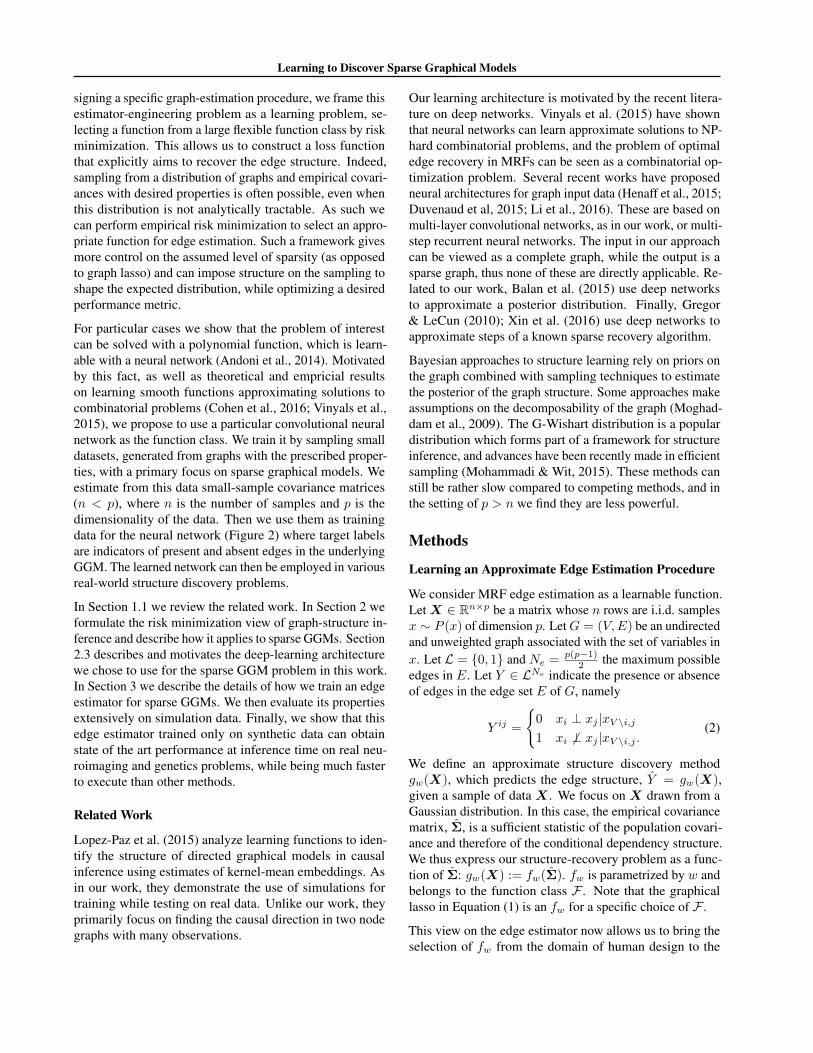
We now describe an efficient architecture for this problemwhich uses a series of shared operations at each edge. Weconsider a feedforward network where each edge i, j is asso-ciated with a vector, oki,j , at each layer k > 0. For each edge,i, j, we start with a neighborhood of the 6 adjacent nodes,i, j, i-1, i+1, j-1, j+1 for which we take all correspondingedge values from the covariance matrix and construct o1i,j .We proceed at each layer to increase the nodes consideredfor each oki,j , the output at each layer progressively increas-ing the receptive field making sure all values associated withthe considered nodes are present. The entries used at eachlayer are illustrated in Figure 1. The receptive field hererefers to the original covariance entries which are accessibleby a given, oki,j (Luo et al., 2010). The equations definingthe process are shown in Figure 1. Here a neural networkfwk is applied at each edge at each layer and a dilation se-quence dk is used. We call a network of this topology aD-Net of depth l. We use dilation here to allow the receptivefield to grow fast, so the network does not need a great dealof layers. We make the following observations:Proposition 2. For general P it is a necessary conditionfor P-consistency that the receptive field of D-Net covers allentries of the covariance, Σ, at any edge it is applied.Proof. Consider nodes i and j and a chain graph such thati and j are adjacent to each other in the matrix but are atthe terminal nodes of the chain graph. One would needto consider all other variables to be able to explain awaythe correlation. Alternatively we can see this directly fromexpanding Eq. (4).

Proposition 3. A p × p matrix Σ will be covered by thereceptive field for a D-Net of depth log2(p) and dk = 2k−1

Proof. The receptive field of a D-Net with dilation sequencedk = 2k−1 of depth l is O(2l). We can see this as oki,j willreceive input from ok−1a,b at the edge of it’s receptive field,effectively doubling it. It now follows that we need at leastlog2(p) layers to cover the receptive field.

Intuitively adjacent edges have a high overlap in theirreceptive fields and can easily share information aboutthe non-overlapping components. This is analogous to aparametrized message passing. For example if edge (i, j) isexplained by node k, as k enters the receptive field of edge(i, j − 1), the path through (i, j) can already be discounted.In terms of Eq. (4) this can correspond to storing computa-tions that can be used by neighbor edges from lower levelsin the recursion.

As fwk is identical for all nodes, we can simultaneouslyimplement all edge predictions efficiently as a convolutionalnetwork. We make sure that to have considered all edgesrelevant to the current set of nodes in the receptive fieldwhich requires us to add values from filters applied at thediagonal to all edges. In Figure 1 we illustrate the nodes


3

4

5

12

13

14

(a)

layer 1, edge 4,13

(b)1

162

15

3

14

4

13

5

12

6

11

7

10

8

9

9

8

10

7

11

6

12

5

13

4

14

3

15

2

16

1

layer 2, edge 4,13

(c)1

162

15

3

14

4

13

5

12

6

11

7

10

8

9

9

8

10

7

11

6

12

5

13

4

14

3

15

2

16

1

o0i,j =pi,j

o1i,j =fw1(o0i,j , o0i-1,j , o

0i,j-1, o

0i+1,j-1, ..)

o2i,j =fw2(o1i,j , o1i-d2,j , o

1i,j-d2

, o1i+d2,j-d2, ..)

oli,j =fwl(ol-1i,j , ol-1i-dl,j

, ol-1i,j-dl, ol-1i+dl,j-dl

..)

yi,j =σ(wl+1oli,j)

Figure 1: (a) Illustration of nodes and edges "seen" at edge 4,13 in layer 1 and (b) Receptive field at layer 1. All entries ingrey show the o0i,j in covariance matrix used to compute o14,13. (c) shows the dilation process and receptive field (red) athigher layers. Finally the equations for each layer output are given, initialized by the covariance entries pi,j

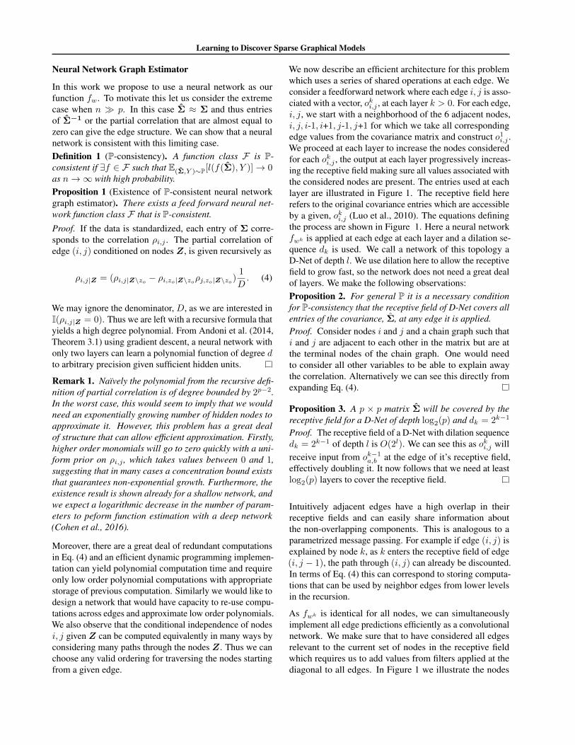
and receptive field considered with respect to the covariancematrix. This also motivates a straightforward implementa-tion using 2D convolutions (adding separate convolutions ati, i and j, j to each i, j at each layer to achieve the specificinput pattern described) shown in Figure 2.

Ultimately our choice of architecture that has shared com-putations and multiple layers is highly scalable as comparedwith a naive fully connected approach and allows leverag-ing existing optimized 2-D convolutions. In preliminarywork we have also considered fully connected layers butthis proved to be much less efficient in terms of storage andscalibility than using deep convolutional networks.

Considering the general n� p case is illustrative. However,the main benefit of making the computations differentiableand learned from data is that we can take advantage of thesparsity and structure assumptions to obtain more efficientresults than naive computation of partial correlation or ma-trix inversion. As n decreases our estimate of ρi,j becomesinexact; a data-driven model that takes better advantage ofthe assumptions on the underlying distribution and can moreaccurately recover the graph structure.

The convolution structure is dependent on the order of thevariables used to build the covariance matrix, which is arbi-trary. Permuting the input data we can obtain another esti-mate of the output. In the experiments, we leverage thesevarious estimate in an ensembling approach, averaging theresults of several permutations of input. We observe that thisgenerally yields a modest increase in accuracy, but that evena single node ordering can show substantially improvedperformance over competing methods in the literature.

ExperimentsOur experimental evaluations focus on the challenging highdimensional settings in which p > n and consider bothsynthetic data and real data from genetics and neuroimaging.In our experiments we explore how well networks trained onparametric samples generalize, both to unseen synthetic dataand to several real world problems. In order to highlight

the generality of the learned networks, we apply the samenetwork to multiple domains. We train networks taking in39, 50, and 500 node graphs. The former sizes are chosenbased on the real data we consider in subsequent sections.We refer to these networks as DeepGraph-39, 50, and 500.In all cases we have 50 feature maps of 3× 3 kernels. The39 and 50 node network with 6 convolutional layers anddk = k+ 1. For the 500 node network with 8 convolutionallayers and dk = 2k+1. We use ReLU activations. The lastlayer has 1× 1 convolution and a sigmoid outputing a valueof 0 to 1 for each edge.

We sample P (X|G) with a sparse prior on P (G) as follows.We first construct a lower diagonal matrix, L, where eachentry has α probability of being zero. Non-zero entries areset uniformly between −c and c. Multiplying LLT gives asparse positive definite precision matrix, Θ. This gives usour P (Θ|G) with a sparse prior on P (G). We sample fromthe Gaussian N (0,Θ−1) to obtain samples of X . Here αcorresponds to a specific sparsity level in the final precisionmatrix, which we set to produce matrices 92− 96% sparseand c chosen so that partial correlations range 0 to 1.

Each network is trained continously with new samples gen-erated until the validation error saturates. For a given preci-sion matrix we generate 5 possible X samples to be used astraining data, with a total of approximately 100K trainingsamples used for each network. The networks are optimizedusing ADAM (Kingma & Ba, 2015) coupled with cross-entropy loss as the objective function (cf. Sec. 2.1). We usebatch normalization at each layer. Additionally, we foundthat using the absolute value of the true partial correlationsas labels, instead of hard binary labels, improves results.

Synthetic Data Evaluation To understand the propertiesof our learned networks, we evaluated them on differentsynthetic data than the ones they were trained on. Morespecifically, we used a completely different third party sam-pler so as to avoid any contamination. We use DeepGraph-39, which takes 4 hours to train, on a variety of settings.The same trained network is utilized in the subsequent neu-roimaging evaluations as well. DeepGraph-500 is also used


Dilated Conv. layers

Conv.layer

1x1 Conv. layer

Standardize

Estimate Covariance

Input Data

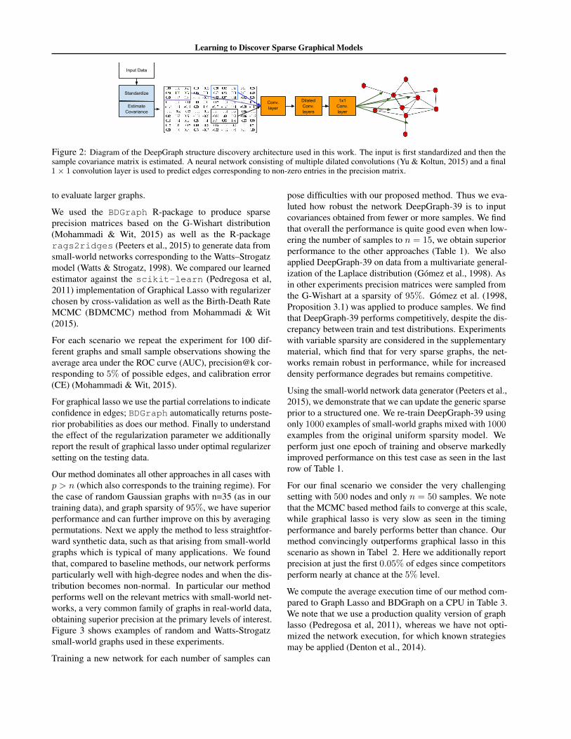
Figure 2: Diagram of the DeepGraph structure discovery architecture used in this work. The input is first standardized and then thesample covariance matrix is estimated. A neural network consisting of multiple dilated convolutions (Yu & Koltun, 2015) and a final1× 1 convolution layer is used to predict edges corresponding to non-zero entries in the precision matrix.

to evaluate larger graphs.

We used the BDGraph R-package to produce sparseprecision matrices based on the G-Wishart distribution(Mohammadi & Wit, 2015) as well as the R-packagerags2ridges (Peeters et al., 2015) to generate data fromsmall-world networks corresponding to the Watts–Strogatzmodel (Watts & Strogatz, 1998). We compared our learnedestimator against the scikit-learn (Pedregosa et al,2011) implementation of Graphical Lasso with regularizerchosen by cross-validation as well as the Birth-Death RateMCMC (BDMCMC) method from Mohammadi & Wit(2015).

For each scenario we repeat the experiment for 100 dif-ferent graphs and small sample observations showing theaverage area under the ROC curve (AUC), precision@k cor-responding to 5% of possible edges, and calibration error(CE) (Mohammadi & Wit, 2015).

For graphical lasso we use the partial correlations to indicateconfidence in edges; BDGraph automatically returns poste-rior probabilities as does our method. Finally to understandthe effect of the regularization parameter we additionallyreport the result of graphical lasso under optimal regularizersetting on the testing data.

Our method dominates all other approaches in all cases withp > n (which also corresponds to the training regime). Forthe case of random Gaussian graphs with n=35 (as in ourtraining data), and graph sparsity of 95%, we have superiorperformance and can further improve on this by averagingpermutations. Next we apply the method to less straightfor-ward synthetic data, such as that arising from small-worldgraphs which is typical of many applications. We foundthat, compared to baseline methods, our network performsparticularly well with high-degree nodes and when the dis-tribution becomes non-normal. In particular our methodperforms well on the relevant metrics with small-world net-works, a very common family of graphs in real-world data,obtaining superior precision at the primary levels of interest.Figure 3 shows examples of random and Watts-Strogatzsmall-world graphs used in these experiments.

Training a new network for each number of samples can

pose difficulties with our proposed method. Thus we eva-luted how robust the network DeepGraph-39 is to inputcovariances obtained from fewer or more samples. We findthat overall the performance is quite good even when low-ering the number of samples to n = 15, we obtain superiorperformance to the other approaches (Table 1). We alsoapplied DeepGraph-39 on data from a multivariate general-ization of the Laplace distribution (Gómez et al., 1998). Asin other experiments precision matrices were sampled fromthe G-Wishart at a sparsity of 95%. Gómez et al. (1998,Proposition 3.1) was applied to produce samples. We findthat DeepGraph-39 performs competitively, despite the dis-crepancy between train and test distributions. Experimentswith variable sparsity are considered in the supplementarymaterial, which find that for very sparse graphs, the net-works remain robust in performance, while for increaseddensity performance degrades but remains competitive.

Using the small-world network data generator (Peeters et al.,2015), we demonstrate that we can update the generic sparseprior to a structured one. We re-train DeepGraph-39 usingonly 1000 examples of small-world graphs mixed with 1000examples from the original uniform sparsity model. Weperform just one epoch of training and observe markedlyimproved performance on this test case as seen in the lastrow of Table 1.

For our final scenario we consider the very challengingsetting with 500 nodes and only n = 50 samples. We notethat the MCMC based method fails to converge at this scale,while graphical lasso is very slow as seen in the timingperformance and barely performs better than chance. Ourmethod convincingly outperforms graphical lasso in thisscenario as shown in Tabel 2. Here we additionally reportprecision at just the first 0.05% of edges since competitorsperform nearly at chance at the 5% level.

We compute the average execution time of our method com-pared to Graph Lasso and BDGraph on a CPU in Table 3.We note that we use a production quality version of graphlasso (Pedregosa et al, 2011), whereas we have not opti-mized the network execution, for which known strategiesmay be applied (Denton et al., 2014).


Experimental Setup Method Prec@5% AUC CEGlasso 0.361 ± 0.011 0.624 ± 0.006 0.07

Gaussian Glasso (optimal) 0.384 ± 0.011 0.639 ± 0.007 0.07Random Graphs BDGraph 0.441 ± 0.011 0.715 ± 0.007 0.28(n = 35, p = 39) DeepGraph-39 0.463 ± 0.009 0.738 ± 0.006 0.07

DeepGraph-39+Perm 0.487 ± 0.010 0.740 ± 0.007 0.07Glasso 0.539 ± 0.014 0.696 ± 0.006 0.07

Gaussian Glasso (optimal) 0.571 ± 0.011 0.704 ± 0.006 0.07Random Graphs BDGraph 0.648 ± 0.012 0.776 ± 0.007 0.16

(n = 100, p = 39) DeepGraph-39 0.567 ± 0.009 0.759 ± 0.006 0.07DeepGraph-39+Perm 0.581± 0.008 0.771± 0.006 0.07

Glasso 0.233 ± 0.010 0.566 ± 0.004 0.07Gaussian Glasso (optimal) 0.263 ± 0.010 0.578 ± 0.004 0.07

Random Graphs BDGraph 0.261 ± 0.009 0.630 ± 0.007 0.41(n = 15, p = 39) DeepGraph-39 0.326 ± 0.009 0.664 ± 0.008 0.08


Laplace Glasso (optimal) 0.337 ± 0.011 0.622 ± 0.006 0.07Random Graphs BDGraph 0.298 ± 0.009 0.687 ± 0.007 0.36(n = 35, p = 39) DeepGraph-39 0.415 ± 0.010 0.711 ± 0.007 0.07


Gaussian Glasso (optimal) 0.453 ± 0.008 0.640 ± 0.004 0.11Small-World Graphs BDGraph 0.428 ± 0.007 0.691 ± 0.003 0.17

(n=35,p=39) DeepGraph-39 0.479 ± 0.007 0.709 ± 0.003 0.11DeepGraph-39+Perm 0.453 ± 0.007 0.712 ± 0.003 0.11

DeepGraph-39+update 0.560 ± 0.008 0.821 ± 0.002 0.11DeepGraph-39+update+Perm 0.555 ± 0.007 0.805 ± 0.003 0.11

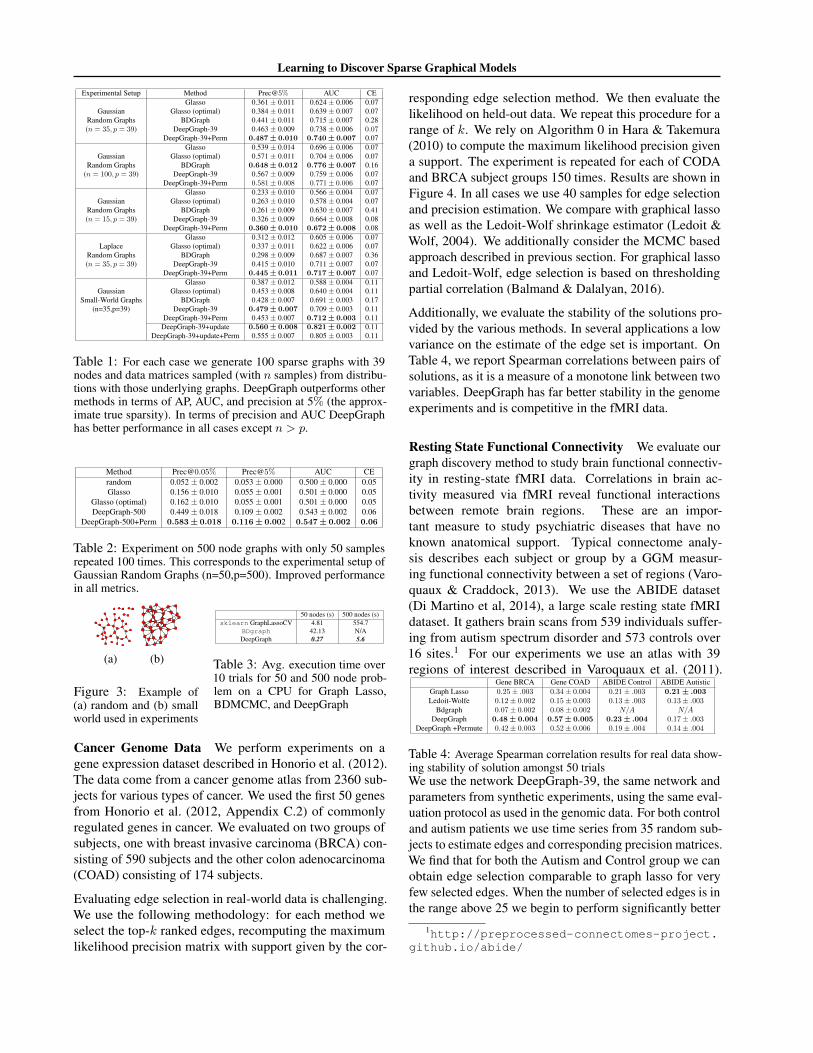
Table 1: For each case we generate 100 sparse graphs with 39nodes and data matrices sampled (with n samples) from distribu-tions with those underlying graphs. DeepGraph outperforms othermethods in terms of AP, AUC, and precision at 5% (the approx-imate true sparsity). In terms of precision and AUC DeepGraphhas better performance in all cases except n > p.

Method [email protected]% Prec@5% AUC CErandom 0.052 ± 0.002 0.053 ± 0.000 0.500 ± 0.000 0.05Glasso 0.156 ± 0.010 0.055 ± 0.001 0.501 ± 0.000 0.05

Glasso (optimal) 0.162 ± 0.010 0.055 ± 0.001 0.501 ± 0.000 0.05DeepGraph-500 0.449 ± 0.018 0.109 ± 0.002 0.543 ± 0.002 0.06

DeepGraph-500+Perm 0.583 ± 0.018 0.116 ± 0.002 0.547 ± 0.002 0.06

Table 2: Experiment on 500 node graphs with only 50 samplesrepeated 100 times. This corresponds to the experimental setup ofGaussian Random Graphs (n=50,p=500). Improved performancein all metrics.

(a) (b)

Figure 3: Example of(a) random and (b) smallworld used in experiments

50 nodes (s) 500 nodes (s)sklearn GraphLassoCV 4.81 554.7

BDgraph 42.13 N/ADeepGraph 0.27 5.6

Table 3: Avg. execution time over10 trials for 50 and 500 node prob-lem on a CPU for Graph Lasso,BDMCMC, and DeepGraph

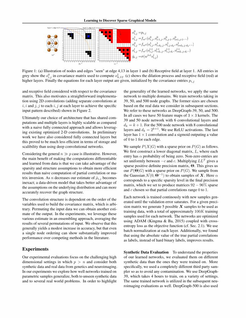
Cancer Genome Data We perform experiments on agene expression dataset described in Honorio et al. (2012).The data come from a cancer genome atlas from 2360 sub-jects for various types of cancer. We used the first 50 genesfrom Honorio et al. (2012, Appendix C.2) of commonlyregulated genes in cancer. We evaluated on two groups ofsubjects, one with breast invasive carcinoma (BRCA) con-sisting of 590 subjects and the other colon adenocarcinoma(COAD) consisting of 174 subjects.

Evaluating edge selection in real-world data is challenging.We use the following methodology: for each method weselect the top-k ranked edges, recomputing the maximumlikelihood precision matrix with support given by the cor-

responding edge selection method. We then evaluate thelikelihood on held-out data. We repeat this procedure for arange of k. We rely on Algorithm 0 in Hara & Takemura(2010) to compute the maximum likelihood precision givena support. The experiment is repeated for each of CODAand BRCA subject groups 150 times. Results are shown inFigure 4. In all cases we use 40 samples for edge selectionand precision estimation. We compare with graphical lassoas well as the Ledoit-Wolf shrinkage estimator (Ledoit &Wolf, 2004). We additionally consider the MCMC basedapproach described in previous section. For graphical lassoand Ledoit-Wolf, edge selection is based on thresholdingpartial correlation (Balmand & Dalalyan, 2016).

Additionally, we evaluate the stability of the solutions pro-vided by the various methods. In several applications a lowvariance on the estimate of the edge set is important. OnTable 4, we report Spearman correlations between pairs ofsolutions, as it is a measure of a monotone link between twovariables. DeepGraph has far better stability in the genomeexperiments and is competitive in the fMRI data.

Resting State Functional Connectivity We evaluate ourgraph discovery method to study brain functional connectiv-ity in resting-state fMRI data. Correlations in brain ac-tivity measured via fMRI reveal functional interactionsbetween remote brain regions. These are an impor-tant measure to study psychiatric diseases that have noknown anatomical support. Typical connectome analy-sis describes each subject or group by a GGM measur-ing functional connectivity between a set of regions (Varo-quaux & Craddock, 2013). We use the ABIDE dataset(Di Martino et al, 2014), a large scale resting state fMRIdataset. It gathers brain scans from 539 individuals suffer-ing from autism spectrum disorder and 573 controls over16 sites.1 For our experiments we use an atlas with 39regions of interest described in Varoquaux et al. (2011).

Gene BRCA Gene COAD ABIDE Control ABIDE AutisticGraph Lasso 0.25± .003 0.34± 0.004 0.21± .003 0.21 ± .003Ledoit-Wolfe 0.12± 0.002 0.15± 0.003 0.13± .003 0.13± .003

Bdgraph 0.07± 0.002 0.08± 0.002 N/A N/ADeepGraph 0.48 ± 0.004 0.57 ± 0.005 0.23 ± .004 0.17± .003

DeepGraph +Permute 0.42± 0.003 0.52± 0.006 0.19± .004 0.14± .004

Table 4: Average Spearman correlation results for real data show-ing stability of solution amongst 50 trialsWe use the network DeepGraph-39, the same network andparameters from synthetic experiments, using the same eval-uation protocol as used in the genomic data. For both controland autism patients we use time series from 35 random sub-jects to estimate edges and corresponding precision matrices.We find that for both the Autism and Control group we canobtain edge selection comparable to graph lasso for veryfew selected edges. When the number of selected edges is inthe range above 25 we begin to perform significantly better

1http://preprocessed-connectomes-project.github.io/abide/

http://preprocessed-connectomes-project.github.io/abide/

http://preprocessed-connectomes-project.github.io/abide/


20 40 60 80 100 120

Edges in support

−72

−71

−70

−69

−68

−67

−66

−65

−64

−63

Log

-Lik

ehoo

dT

est

Dat

aEdge Selection Colon adenocarcinoma Subjects

DeepGraph

DeepGraph+Permute

glasso

ledoit

bayesian

20 40 60 80 100 120

Edges in support

−72

−71

−70

−69

−68

−67

−66

−65

−64

−63

Log

-Lik

ehoo

dT

est

Dat

a

Edge Selection Breast invasive carcinoma Subjects

DeepGraph

DeepGraph+Permute

glasso

ledoit

bayesian

10 20 30 40 50 60 70

Edges in Graph Support

−54.5

−54.0

−53.5

−53.0

−52.5

−52.0

−51.5

−51.0

Ave

rage

Tes

tL

og-L

ikeh

ood

Edge Selection Autism Subjects

10 20 30 40 50 60 70

Edges in Graph Support

−54.5

−54.0

−53.5

−53.0

−52.5

−52.0

−51.5

−51.0

Ave

rage

Tes

tL

og-L

ikeh

ood

Edge Selection Control Subjects

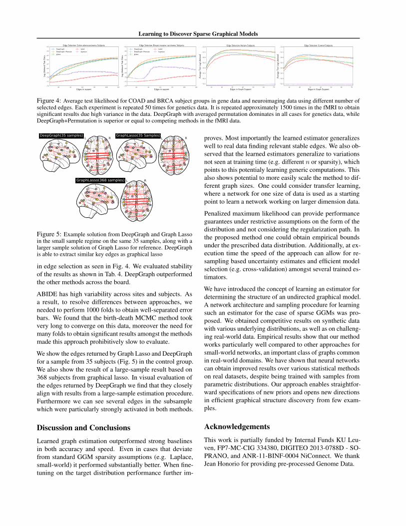
Figure 4: Average test likelihood for COAD and BRCA subject groups in gene data and neuroimaging data using different number ofselected edges. Each experiment is repeated 50 times for genetics data. It is repeated approximately 1500 times in the fMRI to obtainsignificant results due high variance in the data. DeepGraph with averaged permutation dominates in all cases for genetics data, whileDeepGraph+Permutation is superior or equal to competing methods in the fMRI data.

L RDeepGraph(35 samples)

L RGraphLasso(35 Samples)

L RGraphLasso(368 samples)

Figure 5: Example solution from DeepGraph and Graph Lassoin the small sample regime on the same 35 samples, along with alarger sample solution of Graph Lasso for reference. DeepGraphis able to extract similar key edges as graphical lasso

in edge selection as seen in Fig. 4. We evaluated stabilityof the results as shown in Tab. 4. DeepGraph outperformedthe other methods across the board.

ABIDE has high variability across sites and subjects. Asa result, to resolve differences between approaches, weneeded to perform 1000 folds to obtain well-separated errorbars. We found that the birth-death MCMC method tookvery long to converge on this data, moreover the need formany folds to obtain significant results amongst the methodsmade this approach prohibitively slow to evaluate.

We show the edges returned by Graph Lasso and DeepGraphfor a sample from 35 subjects (Fig. 5) in the control group.We also show the result of a large-sample result based on368 subjects from graphical lasso. In visual evaluation ofthe edges returned by DeepGraph we find that they closelyalign with results from a large-sample estimation procedure.Furthermore we can see several edges in the subsamplewhich were particularly strongly activated in both methods.

Discussion and ConclusionsLearned graph estimation outperformed strong baselinesin both accuracy and speed. Even in cases that deviatefrom standard GGM sparsity assumptions (e.g. Laplace,small-world) it performed substantially better. When fine-tuning on the target distribution performance further im-

proves. Most importantly the learned estimator generalizeswell to real data finding relevant stable edges. We also ob-served that the learned estimators generalize to variationsnot seen at training time (e.g. different n or sparsity), whichpoints to this potentialy learning generic computations. Thisalso shows potential to more easily scale the method to dif-ferent graph sizes. One could consider transfer learning,where a network for one size of data is used as a startingpoint to learn a network working on larger dimension data.

Penalized maximum likelihood can provide performanceguarantees under restrictive assumptions on the form of thedistribution and not considering the regularization path. Inthe proposed method one could obtain empirical boundsunder the prescribed data distribution. Additionally, at ex-ecution time the speed of the approach can allow for re-sampling based uncertainty estimates and efficient modelselection (e.g. cross-validation) amongst several trained es-timators.

We have introduced the concept of learning an estimator fordetermining the structure of an undirected graphical model.A network architecture and sampling procedure for learningsuch an estimator for the case of sparse GGMs was pro-posed. We obtained competitive results on synthetic datawith various underlying distributions, as well as on challeng-ing real-world data. Empirical results show that our methodworks particularly well compared to other approaches forsmall-world networks, an important class of graphs commonin real-world domains. We have shown that neural networkscan obtain improved results over various statistical methodson real datasets, despite being trained with samples fromparametric distributions. Our approach enables straightfor-ward specifications of new priors and opens new directionsin efficient graphical structure discovery from few exam-ples.

AcknowledgementsThis work is partially funded by Internal Funds KU Leu-ven, FP7-MC-CIG 334380, DIGITEO 2013-0788D - SO-PRANO, and ANR-11-BINF-0004 NiConnect. We thankJean Honorio for providing pre-processed Genome Data.


ReferencesAndoni, Alexandr, Panigrahy, Rina, Valiant, Gregory, and Zhang,

Li. Learning polynomials with neural networks. In ICML, 2014.Balan, Anoop Korattikara, Rathod, Vivek, Murphy, Kevin, and

Welling, Max. Bayesian dark knowledge. In NIPS, 2015.Balmand, Samuel and Dalalyan, Arnak S. On estimation of the

diagonal elements of a sparse precision matrix. ElectronicJournal of Statistics, 10(1):1551–1579, 2016.

Belilovsky, Eugene, Varoquaux, Gaël, and Blaschko, Matthew B.Hypothesis testing for differences in Gaussian graphical models:Applications to brain connectivity. In NIPS, 2016.

Cai, Tony, Liu, Weidong, and Luo, Xi. A constrained `1 minimiza-tion approach to sparse precision matrix estimation. Journal ofthe American Statistical Association, 106(494):594–607, 2011.

Cohen, Nadav, Sharir, Or, and Shashua, Amnon. On the expressivepower of deep learning: a tensor analysis. In COLT, 2016.

Danaher, Patrick, Wang, Pei, and Witten, Daniela M. The jointgraphical lasso for inverse covariance estimation across multipleclasses. Journal of the Royal Stat. Society(B), 76(2):373–397,2014.

Denton, Emily L, Zaremba, Wojciech, Bruna, Joan, LeCun, Yann,and Fergus, Rob. Exploiting linear structure within convolu-tional networks for efficient evaluation. In NIPS, 2014.

Di Martino et al, Adriana. The autism brain imaging data ex-change: Towards a large-scale evaluation of the intrinsic brainarchitecture in autism. Molecular psychiatry, 19:659, 2014.

Duvenaud et al, David K. Convolutional networks on graphs forlearning molecular fingerprints. In NIPS, 2015.

Friedman, Jerome, Hastie, Trevor, and Tibshirani, Robert. Sparseinverse covariance estimation with the graphical lasso. Bio-statistics, 9(3):432–441, 2008.

Gómez, E, Gomez-Viilegas, MA, and Marin, JM. A multivariategeneralization of the power exponential family of distributions.Commun Stat Theory Methods, 27(3):589–600, 1998.

Gregor, Karol and LeCun, Yann. Learning fast approximations ofsparse coding. In ICML, 2010.

Hara, Hisayuki and Takemura, Akimichi. A localization approachto improve iterative proportional scaling in Gaussian graphicalmodels. Commun Stat Theory Methods, 39(8-9):1643–1654,2010.

Henaff, Mikael, Bruna, Joan, and LeCun, Yann. Deep convolu-tional networks on graph-structured data. arXiv:1506.05163,2015.

Honorio, Jean, Jaakkola, Tommi, and Samaras, Dimitris. On thestatistical efficiency of `1,p multi-task learning of Gaussiangraphical models. arXiv:1207.4255, 2012.

Kingma, Diederik and Ba, Jimmy. Adam: A method for stochasticoptimization. ICLR, 2015.

Lauritzen, Steffen L. Graphical models. Oxford University Press,1996.

Ledoit, Olivier and Wolf, Michael. A well-conditioned estimatorfor large-dimensional covariance matrices. Journal of multivari-ate analysis, 88(2):365–411, 2004.

Lenkoski, Alex. A direct sampler for G-Wishart variates. Stat, 2(1):119–128, 2013.

Li, Yujia, Tarlow, Daniel, Brockschmidt, Marc, and Zemel,Richard. Gated graph sequence neural networks. ICLR, 2016.

Lopez-Paz, David, Muandet, Krikamol, Schölkopf, Bernhard, andTolstikhin, Iliya. Towards a learning theory of cause-effectinference. In ICML, 2015.

Luo, Wenjie, Li, Yujia, Urtasun, Raquel, and Zemel, Richard.Understanding the effective receptive field in deep convolutionalneural networks. In ICML, 2010.

Meinshausen, Nicolai and Bühlmann, Peter. High-dimensional

graphs and variable selection with the lasso. The Annals ofStatistics, pp. 1436–1462, 2006.

Moghaddam, Baback, Khan, Emtiyaz, Murphy, Kevin P, and Mar-lin, Benjamin M. Accelerating Bayesian structural inference fornon-decomposable Gaussian graphical models. In NIPS, 2009.

Mohammadi, Abdolreza and Wit, Ernst C. Bayesian structurelearning in sparse Gaussian graphical models. Bayesian Analy-sis, 10(1):109–138, 2015.

Mohan, Karthik, Chung, Mike, Han, Seungyeop, Witten, Daniela,Lee, Su-In, and Fazel, Maryam. Structured learning of Gaussiangraphical models. In NIPS, pp. 620–628, 2012.

Pedregosa et al, Fabian. Scikit-learn: Machine learning in python.JMLR, 12:2825–2830, 2011.

Peeters, C.F.W., Bilgrau, A.E., and van Wieringen, W.N.rags2ridges: Ridge estimation of precision matrices from high-dimensional data. R package, 2015.

Ravikumar, Pradeep, Wainwright, Martin J, Raskutti, Garvesh, andYu, Bin. High-dimensional covariance estimation by minimiz-ing `1-penalized log-determinant divergence. EJS, 5:935–980,2011.

Ryali et al, Srikanth. Estimation of functional connectivity in fMRIdata using stability selection-based sparse partial correlationwith elastic net penalty. NeuroImage, 59(4):3852–3861, 2012.

Varoquaux, Gaël and Craddock, R Cameron. Learning and com-paring functional connectomes across subjects. NeuroImage,80:405–415, 2013.

Varoquaux, Gaël, Gramfort, Alexandre, Poline, Jean-Baptiste, andThirion, Bertrand. Brain covariance selection: Better individualfunctional connectivity models using population prior. In NIPS,2010.

Varoquaux, Gaël, Gramfort, Alexandre, Pedregosa, Fabian, Michel,Vincent, and Thirion, Bertrand. Multi-subject dictionary learn-ing to segment an atlas of brain spontaneous activity. In IPMI,2011.

Vinyals, Oriol, Fortunato, Meire, and Jaitly, Navdeep. Pointernetworks. In NIPS, 2015.

Wang, Wei, Wainwright, Martin J, and Ramchandran, Kannan.Information-theoretic bounds on model selection for gaussianmarkov random fields. In ISIT, pp. 1373–1377. Citeseer, 2010.

Watts, Duncan J. and Strogatz, Steven H. Collective dynamics of‘small-world’ networks. Nature, 393(6684):440–442, 06 1998.

Xin, Bo, Wang, Yizhou, Gao, Wen, and Wipf, David. Maximalsparsity with deep networks? arXiv preprint arXiv:1605.01636,2016.

Yu, Fisher and Koltun, Vladlen. Multi-scale context aggregation bydilated convolutions. arXiv preprint arXiv:1511.07122, 2015.

learning to discover sparse graphical...

Documents