sparse optimization methodspages.cs.wisc.edu/~swright/talks/sjw-toulouse.pdf1 sparse optimization...

Sparse Optimization Methods

Stephen Wright

University of Wisconsin-Madison

Toulouse, Feb 2009

Stephen Wright (UW-Madison) Sparse Optimization Methods Toulouse, February 2009 1 / 58

1 Sparse OptimizationMotivation for Sparse OptimizationApplications of Sparse OptimizationFormulating Sparse Optimization Problems

2 Compressed Sensing

3 Matrix Completion

4 Composite Minimization Framework

5 Conclusions

+ Adrian Lewis, Ben Recht, Sangkyun Lee.


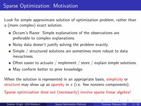
Sparse Optimization: Motivation

Look for simple approximate solution of optimization problem, rather thana (more complex) exact solution.

Occam’s Razor: Simple explanations of the observations arepreferable to complex explanations.

Noisy data doesn’t justify solving the problem exactly.

Simple / structured solutions are sometimes more robust to datainexactness.

Often easier to actuate / implement / store / explain simple solutions.

May conform better to prior knowledge.

When the solution is represented in an appropriate basis, simplicity orstructure may show up as sparsity in x (i.e. few nonzero components).

Sparse optimization does not (necessarily) involve sparse linear algebra!


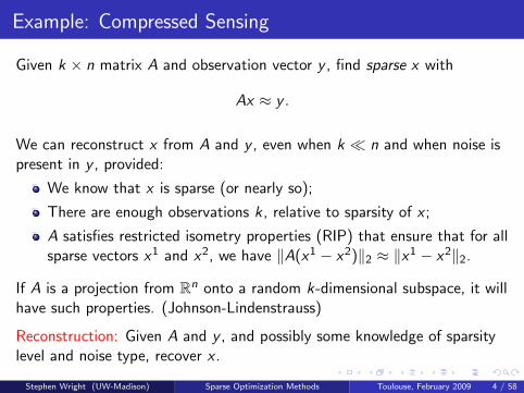
Example: Compressed Sensing

Given k × n matrix A and observation vector y , find sparse x with

Ax ≈ y .

We can reconstruct x from A and y , even when k n and when noise ispresent in y , provided:

We know that x is sparse (or nearly so);

There are enough observations k, relative to sparsity of x ;

A satisfies restricted isometry properties (RIP) that ensure that for allsparse vectors x1 and x2, we have ‖A(x1 − x2)‖2 ≈ ‖x1 − x2‖2.

If A is a projection from Rn onto a random k-dimensional subspace, it willhave such properties. (Johnson-Lindenstrauss)

Reconstruction: Given A and y , and possibly some knowledge of sparsitylevel and noise type, recover x .


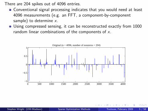
There are 204 spikes out of 4096 entries.

Conventional signal processing indicates that you would need at least4096 measurements (e.g. an FFT, a component-by-componentsample) to determine x .Using compressed sensing, it can be reconstructed exactly from 1000random linear combinations of the components of x .

0 500 1000 1500 2000 2500 3000 3500 4000−1

−0.5

0

0.5

1Original (n = 4096, number of nonzeros = 204)


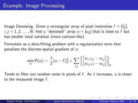
Example: Image Processing

Image Denoising: Given a rectangular array of pixel intensities f = [fij ],i , j = 1, 2, . . . ,N, find a “denoised” array u = [uij ] that is close to f buthas smaller total variation (more cartoon-like).

Formulate as a data-fitting problem with a regularization term thatpenalizes the discrete spatial gradient of u:

minu

P(u) :=λ

2‖u − f ‖22 +

∑i ,j

∥∥∥∥[ui+1,j − ui ,j

ui ,j+1 − ui ,j

]∥∥∥∥2

Tends to filter out random noise in pixels of f . As λ increases, u is closerto the measured image f .


Figure: CAMERAMAN: original (left) and noisy (right)


Figure: Denoised CAMERAMAN: Tol=10−2 (left) and Tol=10−4 (right).


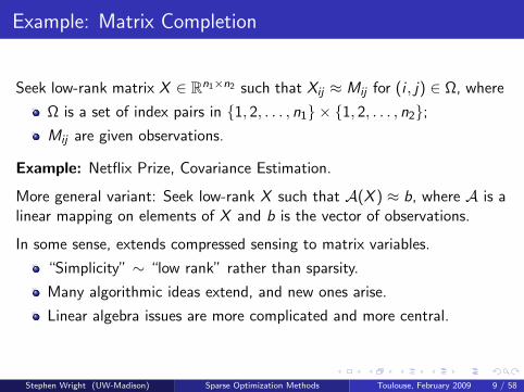
Example: Matrix Completion

Seek low-rank matrix X ∈ Rn1×n2 such that Xij ≈ Mij for (i , j) ∈ Ω, where

Ω is a set of index pairs in 1, 2, . . . , n1 × 1, 2, . . . , n2;Mij are given observations.

Example: Netflix Prize, Covariance Estimation.

More general variant: Seek low-rank X such that A(X ) ≈ b, where A is alinear mapping on elements of X and b is the vector of observations.

In some sense, extends compressed sensing to matrix variables.

“Simplicity” ∼ “low rank” rather than sparsity.

Many algorithmic ideas extend, and new ones arise.

Linear algebra issues are more complicated and more central.


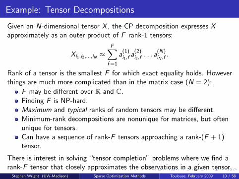
Example: Tensor Decompositions

Given an N-dimensional tensor X , the CP decomposition expresses Xapproximately as an outer product of F rank-1 tensors:

Xi1,i2,...,iN ≈F∑

f =1

a(1)i1,f

a(2)i2,f

. . . a(N)iN ,f .

Rank of a tensor is the smallest F for which exact equality holds. Howeverthings are much more complicated than in the matrix case (N = 2):

F may be different over R and C.

Finding F is NP-hard.

Maximum and typical ranks of random tensors may be different.

Minimum-rank decompositions are nonunique for matrices, but oftenunique for tensors.

Can have a sequence of rank-F tensors approaching a rank-(F + 1)tensor.

There is interest in solving “tensor completion” problems where we find arank-F tensor that closely approximates the observations in a given tensor.


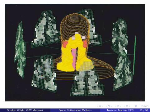
Example: Radiotherapy for Cancer

Deliver radiation from an external device to an internal tumor.

Shape radiation beam, choose angles of delivery so as to deliverprescribed radiation dose to tumor while avoiding dose to surroundingtissue and organs.

Use just a few different beam shapes and angles, to simplify thetreatment, avoid spending too much time on the device, hopefullyreduce the likelihood of treatment errors.


Linear accelerator, showing cone and collimators


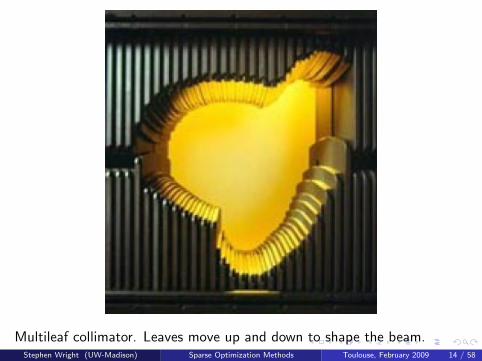
Multileaf collimator. Leaves move up and down to shape the beam.Stephen Wright (UW-Madison) Sparse Optimization Methods Toulouse, February 2009 14 / 58

Class of Examples: Extracting Information from Data

We are drowning in data!

Key challenge: Extract salient information from large data setsefficiently.

What’s “Salient”

Main effects — the essence — not minor effects that possibly overfitthe observationsThe main effects are sometimes complex combinations of the basicones — that is, we are looking for a small number from a potentiallyhuge set — needle in a haystack.The problem is sparse, by our definition.

A few specific instances follow...


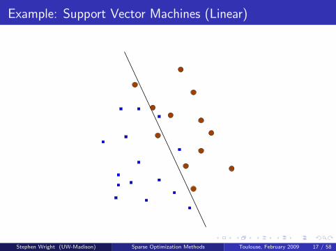
Example: Support Vector Machines (Linear)


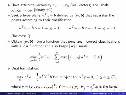
Have attribute vectors x1, x2, . . . , xm (real vectors) and labelsy1, y2, . . . , ym (binary ±1).

Seek a hyperplane wT x − b defined by (w , b) that separates thepoints according to their classification:

wT xi − b >= 1⇒ yi = 1, wT xi − b <= −1⇒ yi = −1

(for most i).

Obtain (w , b) from a function that penalizes incorrect classificationswith a loss function, and also keeps ‖w‖2 small:

min(w ,b)

λ

2wTw +

m∑i=1

max(1− yi [w

T xi − b], 0)

.

Dual formulation:

maxα

eTα− 1

2αTY TKY α subject to αT y = 0, 0 ≤ α ≤ C1,

where y = (y1, y2, . . . , ym)T , Y = diag(y), Kij = xTi xj is the kernel.


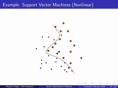
Example: Support Vector Machines (Nonlinear)


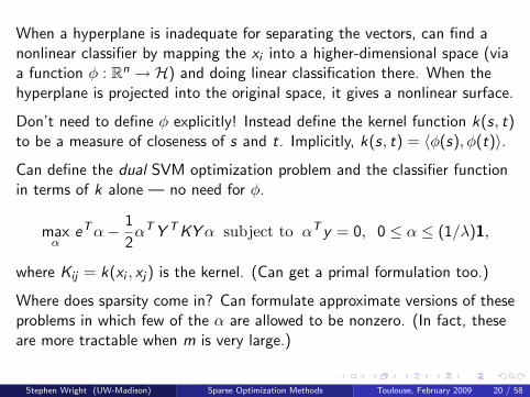
When a hyperplane is inadequate for separating the vectors, can find anonlinear classifier by mapping the xi into a higher-dimensional space (viaa function φ : Rn → H) and doing linear classification there. When thehyperplane is projected into the original space, it gives a nonlinear surface.

Don’t need to define φ explicitly! Instead define the kernel function k(s, t)to be a measure of closeness of s and t. Implicitly, k(s, t) = 〈φ(s), φ(t)〉.

Can define the dual SVM optimization problem and the classifier functionin terms of k alone — no need for φ.

maxα

eTα− 1

2αTY TKY α subject to αT y = 0, 0 ≤ α ≤ (1/λ)1,

where Kij = k(xi , xj) is the kernel. (Can get a primal formulation too.)

Where does sparsity come in? Can formulate approximate versions of theseproblems in which few of the α are allowed to be nonzero. (In fact, theseare more tractable when m is very large.)


Example: Regularized Logistic Regression

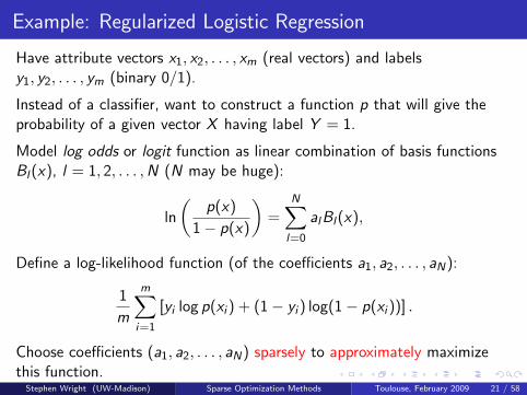
Have attribute vectors x1, x2, . . . , xm (real vectors) and labelsy1, y2, . . . , ym (binary 0/1).

Instead of a classifier, want to construct a function p that will give theprobability of a given vector X having label Y = 1.

Model log odds or logit function as linear combination of basis functionsBl(x), l = 1, 2, . . . ,N (N may be huge):

ln

(p(x)

1− p(x)

)=

N∑l=0

alBl(x),

Define a log-likelihood function (of the coefficients a1, a2, . . . , aN):

1

m

m∑i=1

[yi log p(xi ) + (1− yi ) log(1− p(xi ))] .

Choose coefficients (a1, a2, . . . , aN) sparsely to approximately maximizethis function.


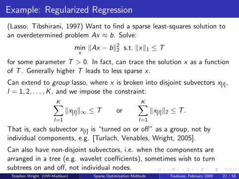
Example: Regularized Regression

(Lasso: Tibshirani, 1997) Want to find a sparse least-squares solution toan overdetermined problem Ax ≈ b. Solve:

minx‖Ax − b‖22 s.t. ‖x‖1 ≤ T

for some parameter T > 0. In fact, can trace the solution x as a functionof T . Generally higher T leads to less sparse x .

Can extend to group lasso, where x is broken into disjoint subvectors x[l ],l = 1, 2, . . . ,K , and we impose the constraint:

K∑l=1

‖x[l ]‖∞ ≤ T orK∑

l=1

‖x[l ]‖2 ≤ T .

That is, each subvector x[l ] is “turned on or off” as a group, not byindividual components, e.g. [Turlach, Venables, Wright, 2005].

Can also have non-disjoint subvectors, i.e. when the components arearranged in a tree (e.g. wavelet coefficients), sometimes wish to turnsubtrees on and off, not individual nodes.


Formulating Sparse Optimization Problems

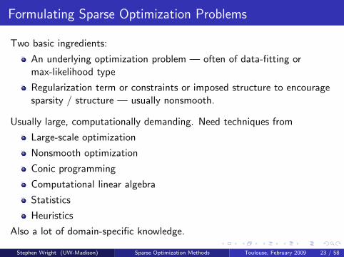
Two basic ingredients:

An underlying optimization problem — often of data-fitting ormax-likelihood type

Regularization term or constraints or imposed structure to encouragesparsity / structure — usually nonsmooth.

Usually large, computationally demanding. Need techniques from

Large-scale optimization

Nonsmooth optimization

Conic programming

Computational linear algebra

Statistics

Heuristics

Also a lot of domain-specific knowledge.


Nonsmooth Norms are Useful!

Consider first a scalar function f : R→ R. Want to find x thatapproximately minimizes f , but accept 0 as an approximate solutionprovided it’s not too far off.

One approach is to add the nonsmooth regularizer |x | with parameterλ > 0, and solve

minx

f (x) + λ|x |

First-order optimality conditions are 0 ∈ ∂f (x), where

∂f (x) =

f ′(x)− λ if x < 0

f ′(0) + λ[−1, 1] if x = 0

f ′(x) + λ if x > 0.

Introduces nonsmoothness at the kink x = 0, making it more “likely” that0 will be chosen as the solution.

The “likelihood” increases as λ increases.Stephen Wright (UW-Madison) Sparse Optimization Methods Toulouse, February 2009 24 / 58

Effect of λ

f(x)


Effect of λ

f(x)+|x|


Effect of λ

f(x)+2|x|


Higher Dimensions

In higher dimensions, if we design nonsmooth functions c(x) that havetheir “kinks” at points that are “sparse” according to our definition, thenthey are suitable regularizers for our problem.

Examples:

c(x) = ‖x‖1 will tend to produce x with few nonzeros.

c(x) = ‖x‖1 is less interesting — kink only when all components arezero (all or nothing).

c(x) = ‖x‖∞ has kinks where components of x are equal — also maynot be interesting for sparsity.

c(x) =∑K

l=1 ‖x[l ]‖2 has kinks where x[l ] = 0 for some l – suitable forgroup sparsity.

Total Variation norm: Has kinks where ui ,j = ui+1,j = ui ,j+1 for somei , j , i.e. where spatial gradient is zero.


Compressed Sensing

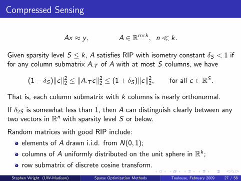
Ax ≈ y , A ∈ Rn×k , n k.

Given sparsity level S ≤ k, A satisfies RIP with isometry constant δS < 1 iffor any column submatrix A·T of A with at most S columns, we have

(1− δS)‖c‖22 ≤ ‖A·T c‖22 ≤ (1 + δS)‖c‖22, for all c ∈ RS .

That is, each column submatrix with k columns is nearly orthonormal.

If δ2S is somewhat less than 1, then A can distinguish clearly between anytwo vectors in Rn with sparsity level S or below.

Random matrices with good RIP include:

elements of A drawn i.i.d. from N(0, 1);

columns of A uniformly distributed on the unit sphere in Rk ;

row submatrix of discrete cosine transform.


RIP and Tractability

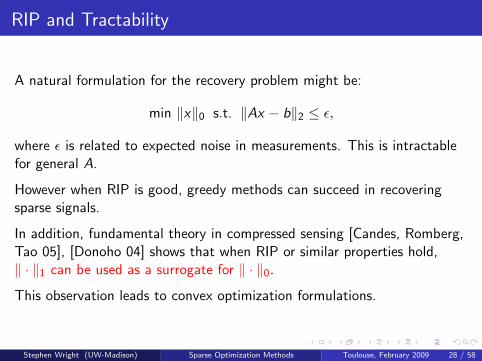
A natural formulation for the recovery problem might be:

min ‖x‖0 s.t. ‖Ax − b‖2 ≤ ε,

where ε is related to expected noise in measurements. This is intractablefor general A.

However when RIP is good, greedy methods can succeed in recoveringsparse signals.

In addition, fundamental theory in compressed sensing [Candes, Romberg,Tao 05], [Donoho 04] shows that when RIP or similar properties hold,‖ · ‖1 can be used as a surrogate for ‖ · ‖0.

This observation leads to convex optimization formulations.


Optimization Formulations of the Recovery Problem

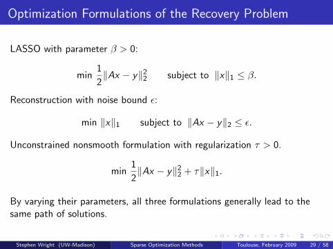
LASSO with parameter β > 0:

min1

2‖Ax − y‖22 subject to ‖x‖1 ≤ β.

Reconstruction with noise bound ε:

min ‖x‖1 subject to ‖Ax − y‖2 ≤ ε.

Unconstrained nonsmooth formulation with regularization τ > 0.

min1

2‖Ax − y‖22 + τ‖x‖1.

By varying their parameters, all three formulations generally lead to thesame path of solutions.


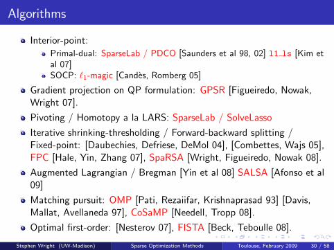
Algorithms

Interior-point:

Primal-dual: SparseLab / PDCO [Saunders et al 98, 02] l1 ls [Kim etal 07]SOCP: `1-magic [Candes, Romberg 05]

Gradient projection on QP formulation: GPSR [Figueiredo, Nowak,Wright 07].

Pivoting / Homotopy a la LARS: SparseLab / SolveLasso

Iterative shrinking-thresholding / Forward-backward splitting /Fixed-point: [Daubechies, Defriese, DeMol 04], [Combettes, Wajs 05],FPC [Hale, Yin, Zhang 07], SpaRSA [Wright, Figueiredo, Nowak 08].

Augmented Lagrangian / Bregman [Yin et al 08] SALSA [Afonso et al09]

Matching pursuit: OMP [Pati, Rezaiifar, Krishnaprasad 93] [Davis,Mallat, Avellaneda 97], CoSaMP [Needell, Tropp 08].

Optimal first-order: [Nesterov 07], FISTA [Beck, Teboulle 08].


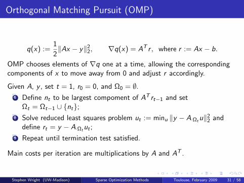
Orthogonal Matching Pursuit (OMP)

q(x) :=1

2‖Ax − y‖22, ∇q(x) = AT r , where r := Ax − b.

OMP chooses elements of ∇q one at a time, allowing the correspondingcomponents of x to move away from 0 and adjust r accordingly.

Given A, y , set t = 1, r0 = 0, and Ω0 = ∅.1 Define nt to be largest compoment of AT rt−1 and set

Ωt = Ωt−1 ∪ nt;2 Solve reduced least squares problem ut := minu ‖y − A·Ωtu‖22 and

define rt = y − A·Ωtut ;

3 Repeat until termination test satisfied.

Main costs per iteration are multiplications by A and AT .


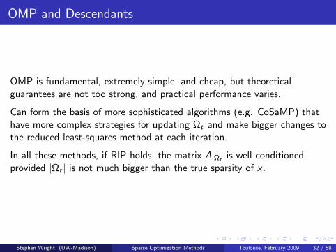
OMP and Descendants

OMP is fundamental, extremely simple, and cheap, but theoreticalguarantees are not too strong, and practical performance varies.

Can form the basis of more sophisticated algorithms (e.g. CoSaMP) thathave more complex strategies for updating Ωt and make bigger changes tothe reduced least-squares method at each iteration.

In all these methods, if RIP holds, the matrix A·Ωt is well conditionedprovided |Ωt | is not much bigger than the true sparsity of x .


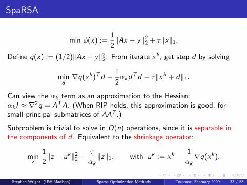
SpaRSA

min φ(x) :=1

2‖Ax − y‖22 + τ‖x‖1.

Define q(x) := (1/2)‖Ax − y‖22. From iterate xk , get step d by solving

mind∇q(xk)Td +

1

2αkdTd + τ‖xk + d‖1.

Can view the αk term as an approximation to the Hessian:αk I ≈ ∇2q = ATA. (When RIP holds, this approximation is good, forsmall principal submatrices of AAT .)

Subproblem is trivial to solve in O(n) operations, since it is separable inthe components of d . Equivalent to the shrinkage operator:

minz

1

2‖z − uk‖22 +

τ

αk‖z‖1, with uk := xk − 1

αk∇q(xk).


Choosing αk

By choosing αk greater than a threshold value α at every iteration,can guarantee convergence, but slowly.

Can use a Barzilai-Borwein (BB) strategy: choose αk it to mimic thetrue Hessian ATA over the step just taken. e.g. do a least squares fitto:

[xk − xk−1] ≈ α−1k [∇q(xk)−∇q(xk−1)].

Generally non-monotone.

Cyclic BB variants: e.g. update αk only every 3rd iteration.

Get monotone variants by backtracking: set αk ← 2αk repeatedlyuntil a decrease in objective is obtained.


SpaRSA Implementation and Properties

Exploits warm starts well.

Problem is harder to solve for smaller τ (corresponding to morenonzeros in x). Performance improved greatly by continuation:

Choose initial τ0 ≤ ‖AT y‖∞ and decreasing sequenceτ0 > τ1 > τ2 > . . . > τfinal > 0, where τfinal is the target final value.Solve for τ equal to each element in sequence, using previous solutionas the warm start.

Debiasing: After convergence of the main algorithm, fix nonzero set(support) in x and minimize ‖Ax − b‖22 over this reduced set.

Can make large changes to the active manifold on a single step (likeinterior-point, unlike pivoting).

Each iteration is cheap: one multiplication each with A or AT


Matrix Completion

Seek low-rank matrix X ∈ Rn1×n2 such that A(X ) ≈ b, where A is a linearmapping on elements of X and b is the vector of observations.

In some sense, extends matrix completion is compressed sensing on matrixvariables. Linear algebra is more complicated.

Can formulate asminX

rank(X ) s.t. A(X ) = b

for exact observations, or

minX

rank(X ) s.t. ‖A(X )− b‖ ≤ ε

for noisy observations.


Matrix Completion Formulations

To get a convex optimization formulation, replace rank(X ) by its convexenvelope on the set X | ‖X‖2 ≤ 1, which is the nuclear norm ‖X‖∗defined by

‖X‖∗ =

n2∑i=1

σi (X ),

where σi (X ) is the ith singular value of X . This is a nonsmooth convexfunction of X .

Obtain formulations

minX‖X‖∗ s.t. A(X ) = b (1)

and

minX

τ‖X‖∗ +1

2‖A(X )− b‖22.


Algorithms like SpaRSA

Obtain an extension of the SpaRSA approach by using αk I to approximateA∗A. Obtain steps from the shrinkage operator by solving:

minZ

τ

αk‖Z‖∗ +

1

2‖Z − Y k‖2F ,

where

Y k := X k − 1

αkA∗(A(X k)− b).

e.g. [Ma, Goldfarb, Chen, 08]. Can prove convergence for αk sufficientlylarge (uniformly greater than λmax(A∗A)/2).

Can enhance by similar strategies as in compressed sensing:

Continuation

Barzilai-Borwein αk , nonmonotonicity

Debiasing.


Implementing Shrinking Methods

Main operation is the shrinkage operator:

minZ

ν‖Z‖∗ +1

2‖Z − Y ‖2F ,

which can be solved via an SVD of Y . Calculate Y = UΣV T , then definediagonal matrix Σ(ν) by

Σ(ν)ii = max(Σii − ν, 0),

and set Z = UΣ(ν)V T . Expensive for problems of interesting size.

Need for approximate SVD strategies.

possibly based on sampling;

possibly using Lanczos iterations;

possibly exploiting the fact that we often need only a few leadingsingular values and vectors

See [Halko, Martinsson, Tropp 09] for a review of sampling-basedapproximate factorizations.


Explicit Parametrization of X

From [Recht, Fazel, Parrilo 07] and earlier work of Burer, Monteiro, Choiin SDP setting.

Choose target rank r and approximate X by LRT , where L ∈ Rn1×r andR ∈ Rn1×r are the unknowns in the problem. For the formulation:

minX‖X‖∗ s.t. A(X )− b,

we have the following equivalent formulation:

minL,R

1

2

(‖L‖2F + ‖R‖2F

)s.t.A(LRT ) = b.

A nonconvex minimization problem. Local solutions can be found by e.g.the method of multipliers [RFP 07], [Recht 08] using nonlinear conjugategradient (modified Polak-Ribiere) for the subproblems.

Can perform exact line search with a quartic rootfinder [Burer, Choi 06].


Explicit Parametrization: Noisy Formulation

minL,R

τ(‖L‖2F + ‖R‖2F

)+

1

2

∥∥∥A(LRT )− b∥∥∥2

2.

Again, can use nonlinear conjugate gradient with exact line search, andcan do continuation on τ .

No need for SVD. Implementations are easy.

Local minima? [Burer 06] shows that (in an SDP setting) provided ris chosen large enough, the method should not converge to a localsolution — only the global solution.

Performance degrades when rank is overestimated, probably becauseof degeneracy.

Investigations of this approach are ongoing.


Summarizing: Tools Used for Matrix Completion

Formulation Tools:

Nuclear norm as a proxy for rank.Lagrangian theory (equivalence of different formulations).No local solutions, despite nonconvexity.

Optimization Tools:

Operator splitting (the basis of IST)Gradient projection(Optimal) gradient and subgradient methodsAugmented LagrangianAlgorithms for large-scale nonlinear unconstrained problems (nonlinearCG, L-BFGS)Semidefinite programmingHandling of degeneracy

Linear Algebra Tools:

SVDApproximate SVD via samplingLanczos


Composite Minimization Framework

[Lewis, Wright 08] Develop a general algorithmic framework andsupporting theory, for extension of SpaRSA-like approaches to a muchwider class of problems.

minx

h(c(x))

vector function c : Rn → Rm is smooth;

scalar function h : Rm → R usually nonsmooth.

In most of the analysis, we allow h to be

extended-valued (to enforce some constraints explicitly)

subdifferentially regularity or prox-regular.

Many applications have h convex — the analysis is much simpler in thiscase.


Examples

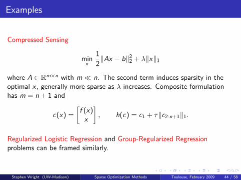
Compressed Sensing

minx

1

2‖Ax − b‖22 + λ‖x‖1

where A ∈ Rm×n with m n. The second term induces sparsity in theoptimal x , generally more sparse as λ increases. Composite formulationhas m = n + 1 and

c(x) =

[f (x)x

], h(c) = c1 + τ‖c2:n+1‖1.

Regularized Logistic Regression and Group-Regularized Regressionproblems can be framed similarly.


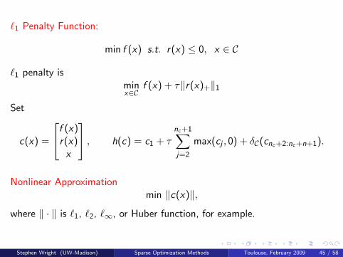
`1 Penalty Function:

min f (x) s.t. r(x) ≤ 0, x ∈ C

`1 penalty isminx∈C

f (x) + τ‖r(x)+‖1

Set

c(x) =

f (x)r(x)x

, h(c) = c1 + τ

nc+1∑j=2

max(cj , 0) + δC(cnc+2:nc+n+1).

Nonlinear Approximationmin ‖c(x)‖,

where ‖ · ‖ is `1, `2, `∞, or Huber function, for example.


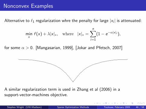
Nonconvex Examples

Alternative to `1 regularization whre the penalty for large |xi | is attenuated:

minx

f (x) + λ|x |∗, where |x |∗ =n∑

i=1

(1− e−α|x |i ),

for some α > 0. [Mangasarian, 1999], [Jokar and Pfetsch, 2007]

A similar regularization term is used in Zhang et al (2006) in asupport-vector-machines objective.


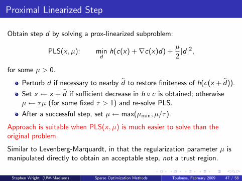
Proximal Linearized Step

Obtain step d by solving a prox-linearized subproblem:

PLS(x , µ): mind

h(c(x) +∇c(x)d) +µ

2|d |2,

for some µ > 0.

Perturb d if necessary to nearby d to restore finiteness of h(c(x + d)).

Set x ← x + d if sufficient decrease in h c is obtained; otherwiseµ← τµ (for some fixed τ > 1) and re-solve PLS.

After a successful step, set µ← max(µmin, µ/τ).

Approach is suitable when PLS(x , µ) is much easier to solve than theoriginal problem.

Similar to Levenberg-Marquardt, in that the regularization parameter µ ismanipulated directly to obtain an acceptable step, not a trust region.


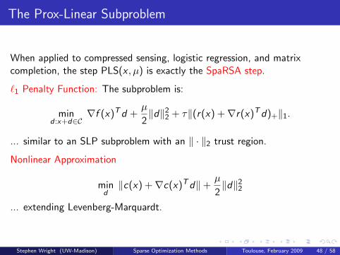
The Prox-Linear Subproblem

When applied to compressed sensing, logistic regression, and matrixcompletion, the step PLS(x , µ) is exactly the SpaRSA step.

`1 Penalty Function: The subproblem is:

mind :x+d∈C

∇f (x)Td +µ

2‖d‖22 + τ‖(r(x) +∇r(x)Td)+‖1.

... similar to an SLP subproblem with an ‖ · ‖2 trust region.

Nonlinear Approximation

mind‖c(x) +∇c(x)Td‖+

µ

2‖d‖22

... extending Levenberg-Marquardt.


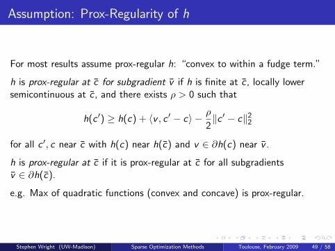
Assumption: Prox-Regularity of h

For most results assume prox-regular h: “convex to within a fudge term.”

h is prox-regular at c for subgradient v if h is finite at c , locally lowersemicontinuous at c , and there exists ρ > 0 such that

h(c ′) ≥ h(c) + 〈v , c ′ − c〉 − ρ

2‖c ′ − c‖22

for all c ′, c near c with h(c) near h(c) and v ∈ ∂h(c) near v .

h is prox-regular at c if it is prox-regular at c for all subgradientsv ∈ ∂h(c).

e.g. Max of quadratic functions (convex and concave) is prox-regular.


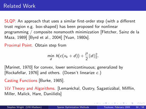
Related Work

SLQP. An approach that uses a similar first-order step (with a differenttrust region e.g. box-shaped) has been proposed for nonlinearprogramming / composite nonsmooth minimization [Fletcher, Sainz de laMaza, 1989] [Byrd et al., 2004] [Yuan, 1980s].

Proximal Point. Obtain step from

mind

h(c(xk + d)) +µ

2‖d‖22.

[Marinet, 1970] for convex, lower semicontinuous; generalized by[Rockafellar, 1976] and others. (Doesn’t linearize c .)

Casting Functions [Burke, 1985].

VU Theory and Algorithms. [Lemarechal, Oustry, Sagastizabal, Mifflin,Miller, Malick, Hare, Daniilidis]


Result: Existence of Solution to PLS

Need a regularity (transversality) condition at critical point x :

∂∞h(c) ∩ null(∇c(x)∗) = 0,

where ∂∞h is the “horizon subgradient” consisting of directions alongwhich h grows faster than any linear function.

Need µ larger than a threshold µ that quantifies the nonconvexity of h atc = c(x).

Then for x near x , we have a local solution d of PLS with d = O(|x − x |).

If xr → x and µr > µ, and either µr |xr − x |2 → 0 or h(c(xr ))→ h(c(x)),we have

h(c(xr ) +∇c(xr )dr )→ h(c(x)).


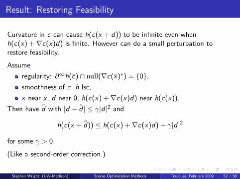
Result: Restoring Feasibility

Curvature in c can cause h(c(x + d)) to be infinite even whenh(c(x) +∇c(x)d) is finite. However can do a small perturbation torestore feasibility.

Assume

regularity: ∂∞h(c) ∩ null(∇c(x)∗) = 0,smoothness of c , h lsc,

x near x , d near 0, h(c(x) +∇c(x)d) near h(c(x)).

Then have d with |d − d | ≤ γ|d |2 and

h(c(x + d)) ≤ h(c(x) +∇c(x)d) + γ|d |2

for some γ > 0.

(Like a second-order correction.)


Result: Multiplier Convergence, Uniqueness

The “multipliers” vr that satisfy

0 = ∇c(xr )∗vr + µrdr

vr ∈ ∂h(c(xr ) +∇c(xr )dr )

are bounded and converge to a unique value when a stronger condition(analogous to LICQ) holds:

par ∂h(c(x)) ∩Null∇c(x)∗ = 0.

When this condition holds, the PLS solution dr near 0 is unique.


Active Manifold Identification

In constrained optimization it is useful to be able to identify the activeconstraints at the solution x∗, before x∗ itself is known. Can thusaccelerate local convergence, improve robustness of algorithms.

In the setting h(c(x)), we look for manifolds in c-space along which h issmooth:

M = c | h|Mis smooth.

When x∗ is such that c(x∗) lies on such a manifold, and when we replace

criticality: ∂h(c) ∩ null (∇c(x)∗) 6= ∅by strict criticality: ri ∂h(c) ∩ null (∇c(x)∗) 6= ∅,

(like strict complementarity) along with other conditions, then

c(xr ) +∇c(xr )dr ∈M

for all r sufficiently large. Also, stay on M after the “efficient projection.”Stephen Wright (UW-Madison) Sparse Optimization Methods Toulouse, February 2009 54 / 58

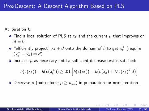
ProxDescent: A Descent Algorithm Based on PLS

At iteration k:

Find a local solution of PLS at xk and the current µ that improves ond = 0;

“efficiently project” xk + d onto the domain of h to get x+k (require

(x+k − xk) ≈ d).

Increase µ as necessary until a sufficient decrease test is satisfied:

h(c(xk))− h(c(x+k )) ≥ .01

[h(c(xk))− h(c(xk) +∇c(xk)Td)

]Decrease µ (but enforce µ ≥ µmin) in preparation for next iteration.


Convergence

Roughly:

The algorithm can step away from a non-stationary point: Thesolution of PLS(x , µ) is accepted for µ large enough.

Cannot have accumulation at noncritical points that are nice (i.e.where h is subdifferentially regular and transversality holds).

See paper for details.


Extensions

Nonmonotone algorithms? Barzilai-Borwein choices of µ.

Second-order enhancements. Use the PLS problem to identify asurface, then take a step along that surface with “real” second-orderinformation: Newton-like step for h(c(x))|M.

Inexact variants.

Regularizers other than (µ/2)|d |2.


Conclusions

Sparse optimization draws on many areas of optimization, linearalgebra, and statistics as well as the underlying application areas.

There is some commonality across different areas that can beabstracted and analyzed.

Much work remains!


sparse optimization methodspages.cs.wisc.edu/~swright/talks/sjw-toulouse.pdf1 sparse optimization...

Documents