learning theory of distributed spectral algorithms · learning theory of distributed spectral...
TRANSCRIPT

Learning Theory of Distributed Spectral Algorithms
Zheng-Chu Guo1 & Shao-Bo Lin2 & Ding-Xuan Zhou2
1. School of Mathematical Sciences, Zhejiang University, Hangzhou 310027, China
E-mail: [email protected]
2. Department of Mathematics, City University of Hong Kong, Kowloon, Hong
Kong, China
E-mail: [email protected], [email protected]
Abstract. Spectral algorithms have been widely used and studied in learning theory
and inverse problems. This paper is concerned with distributed spectral algorithms,
for handling big data, based on a divide-and-conquer approach. We present a learning
theory for these distributed kernel-based learning algorithms in a regression framework
including nice error bounds and optimal minimax learning rates achieved by means
of a novel integral operator approach and a second order decomposition of inverse
operators. Our quantitative estimates are given in terms of regularity of the regression
function, effective dimension of the reproducing kernel Hilbert space, and qualification
of the filter function of the spectral algorithm. They do not need any eigenfunction or
noise conditions and are better than the existing results even for the classical family
of spectral algorithms.
Keywords: Distributed learning, Spectral algorithm, Integral operator, Learning rate
Submitted to: Inverse Problems
1. Introduction
In the big data era, data of high volume may necessarily be stored distributively across
multiple servers rather than on one machine. This makes many traditional learning
algorithms requiring access to the entire data set infeasible. Distributed learning, based
on a divide-and-conquer approach, provides a promising way to tackle this problem and
therefore has recently triggered enormous research activities [13, 15, 22]. This strategy
applies a specific learning algorithm to one data subset on each server, to produce an
individual output (function), and then synthesizes a global output by utilizing some
average of the individual outputs. The learning performance of distributed learning has
been observed in many practical applications to be as good as that of a big machine
which could process the whole data. We are interested in error analysis of such learning
algorithms.

Learning Theory of Distributed Spectral Algorithms 2
Distributed learning with kernel-based regularized least squares was studied in [23],
and optimal (minimax) learning rates were derived with a matrix analysis approach
by making full use of the linearity of the algorithm under some assumptions on
eigenfunctions of the integral operator associated with the kernel. These assumptions
were successfully removed in the recent paper [11] with an integral operator approach
and also by the linearity of the least squares algorithm.
In this paper, we consider a family of more general learning algorithms, spectral
algorithms, and present a learning theory for distributed spectral algorithms. In
particular, optimal learning rates will be provided by means of a novel integral operator
approach. As a by-product, for the classical spectral algorithms for regression, we shall
improve the existing learning rates in the literature by removing a logarithmic factor
and give optimal learning rates.
Spectral algorithms were proposed to solve ill-posed linear inverse problems (see
e.g. [8]) and employed [12, 2] for regression by noticing connections between learning
theory and inverse problems [7]. For learning functions on a compact metric space
X (input space), a spectral algorithm is defined in terms of a Mercer (continuous,
symmetric and positive semidefinite) kernel K : X ×X → R with κ =√
supx∈X K(x, x)
and a filter function gλ : [0, κ2] → R with a parameter λ > 0 acting on spectra of
empirical integral operators. For a sample D = {(xi, yi)}Ni=1 with yi ∈ Y ⊆ R (output
space), the empirical integral operator LK,D associated with the kernel K and the input
data D(x) = {x1, · · · , xN} is defined on the reproducing kernel Hilbert space (RKHS)
(HK , 〈, 〉K) associated with K by
LK,D(f) =1
|D|∑
x∈D(x)
f(x)Kx, f ∈ HK ,
where Kx = K(·, x) and |D| = N denotes the cardinality of D. Given the kernel K, the
filter function gλ, and the sample D, the spectral algorithm is defined by
fD,λ = gλ(LK,D)1
|D|∑
(x,y)∈D
yKx. (1)
Here gλ(LK,D) is an operator on HK defined by spectral calculus: if {(σx
i , φx
i )i} is a set
of normalized eigenpairs of LK,D with the eigenfunctions {φx
i }i forming an orthonormal
basis of HK , then gλ(LK,D) =∑
i gλ(σx
i )φx
i ⊗ φx
i =∑
i gλ(σx
i )〈·, φx
i 〉Kφx
i . This operator
acts on the function fDρ := 1
|D|∑
(x,y)∈D yKx = 1N
∑Ni=1 yiKxi
∈ HK to produce the
output function fD,λ ∈ HK of spectral algorithm (1).
We take a regression framework in learning theory modelled with a probability
measure ρ on Z := X × Y , and assume throughout the paper that a random sample
D = {(xi, yi)}Ni=1 is drawn independently according to ρ. The learning problem for
regression aims at estimating the regression function fρ : X → R defined by conditional
means as
fρ(x) =
∫
Yydρ(y|x), x ∈ X ,

Learning Theory of Distributed Spectral Algorithms 3
where ρ(y|x) is the conditional distribution of ρ at x. The output function fD,λ produced
by spectral algorithm (1) is a good estimator of the regression function fρ when the filter
function gλ is chosen properly and the size N of the sample D is large enough.
As a kernel method, spectral algorithm (1) implements learning tasks in the
hypothesis space HK . What is special about this hypothesis space is its reproducing
property asserting that f(x) = 〈f, Kx〉K for any f ∈ HK and x ∈ X . It tells us that
the empirical integral operator satisfies LK,D(f) = 1|D|∑
x∈D(x)〈f, Kx〉KKx. So LK,D is a
finite-rank positive operator on HK , and its spectrum is contained in the interval [0, κ2]
since ‖Kx‖K =√
K(x, x) ≤ κ. Expressing LK,D in terms of its normalized eigenpairs
{(σx
i , φx
i )i} as LK,D =∑
i σx
i 〈·, φx
i 〉Kφx
i , we see that the filter function gλ acting on LK,D
provides an approximate inverse gλ(LK,D) =∑
i gλ(σx
i )〈·, φx
i 〉Kφx
i of LK,D by regularizing
the eigenvalue reciprocal 1σx
ito gλ(σ
x
i ).
Let ρX be the marginal distribution of ρ on X and (L2ρ
X, ‖ · ‖ρ) be the Hilbert space
of ρX square integrable functions on X . Define the integral operator LK on HK or L2ρX
associated with the Mercer kernel K by
LK(f) =
∫
X
f(x)KxdρX .
When the sample size N is large, the function fDρ = 1
N
∑Ni=1 yiKxi
∈ HK is a good
approximation of its mean∫
Z yKxdρ =∫
X fρ(x)KxdρX = LK(fρ) and the empirical
integral operator LK,D approximates LK well. Hence spectral algorithm (1) produces
a good estimator fD,λ = gλ(LK,D)fDρ of the regression function fρ when fρ ∈ HK and
gλ(LK,D) is an approximate inverse of LK,D or LK .
Let us illustrate the role in inverting LK,D approximately of the filter function gλ
as an approximation of the reciprocal function 1σ
by describing two typical spectral
algorithms, Tikhonov regularization or kernel-based regularized least squares algorithm
and spectral cut-off [2, 12, 18].
Example 1. (Tikhonov Regularization) This spectral algorithm has a filter
function gλ : [0, κ2] → R with a parameter λ > 0 given by gλ(σ) = 1σ+λ
. Its output
function fD,λ equals the solution to the following regularized least squares minimization
problem
fD,λ = arg minf∈HK
{
1
N
N∑
i=1
(f(xi) − yi)2 + λ‖f‖2
K
}
. (2)
To see this, we use the sampling operator Sx : HK → RN defined [16] by Sx(f) =
(f(xi))Ni=1 = (〈f, Kxi
〉K)Ni=1, where the inner product on RN is the normalized one
given by 〈c, c〉RN = 1N
∑Ni=1 cici for c = (ci)
Ni=1, c = (ci)
Ni=1 ∈ RN . If we denote
y = (yi)Ni=1 ∈ RN , then the minimization problem (2) can be expressed as
fD,λ = arg minf∈HK
{
‖Sx(f) − y‖2RN + λ‖f‖2
K
}
,
and its unique solution [8] is fD,λ =(
STxSx + λI
)−1ST
xy. Note that the adjoint
operator STx
: RN → HK is given by STx(c) = 1
N
∑Ni=1 ciKxi
for c ∈ RN . Hence
Learning Theory of Distributed Spectral Algorithms 4
STxSx(f) = 1
N
∑Ni=1 f(xi)Kxi
= LK,D(f) for f ∈ HK , and STxy = 1
N
∑Ni=1 yiKxi
= fDρ .
These identities tell us that fD,λ defined by (2) equals (LK,D + λI)−1 fDρ = gλ(LK,D)fD
ρ ,
the expression in (1) when gλ(σ) = 1λ+σ
.
It is well-known that when λ = 0, the minimization problem (2) is ill-posed and its
solution is not unique in general. This can also be seen from the expression (1) since the
operator LK,D =∑
i σx
i 〈·, φx
i 〉Kφx
i is not invertible and the operator g0(LK,D) = L−1K,D
is not well-defined. When λ > 0, the minimization problem (2) becomes well-posed
and its unique solution is given by means of the operator gλ(LK,D) = (LK,D + λI)−1 =∑
i1
σx
i+λ
〈·, φx
i 〉Kφx
i . Here the filter function gλ maps the eigenvalue σx
i ∈ [0, κ2] in the
spectrum of LK,D to a regularized reciprocal 1σx
i +λinstead of the reciprocal itself.
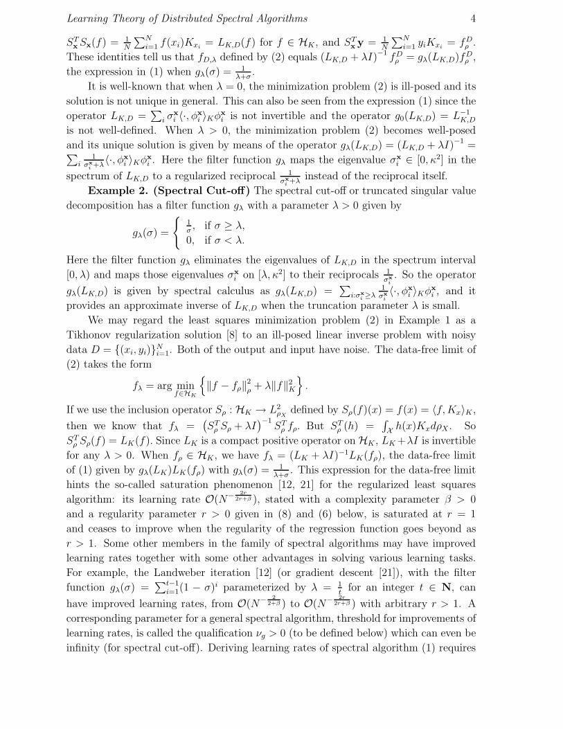
Example 2. (Spectral Cut-off) The spectral cut-off or truncated singular value
decomposition has a filter function gλ with a parameter λ > 0 given by
gλ(σ) =
{
1σ, if σ ≥ λ,
0, if σ < λ.
Here the filter function gλ eliminates the eigenvalues of LK,D in the spectrum interval
[0, λ) and maps those eigenvalues σx
i on [λ, κ2] to their reciprocals 1σx
i. So the operator
gλ(LK,D) is given by spectral calculus as gλ(LK,D) =∑
i:σx
i ≥λ1
σx
i〈·, φx
i 〉Kφx
i , and it
provides an approximate inverse of LK,D when the truncation parameter λ is small.
We may regard the least squares minimization problem (2) in Example 1 as a
Tikhonov regularization solution [8] to an ill-posed linear inverse problem with noisy
data D = {(xi, yi)}Ni=1. Both of the output and input have noise. The data-free limit of
(2) takes the form
fλ = arg minf∈HK
{
‖f − fρ‖2ρ + λ‖f‖2
K
}
.
If we use the inclusion operator Sρ : HK → L2ρX
defined by Sρ(f)(x) = f(x) = 〈f, Kx〉K ,
then we know that fλ =(
STρ Sρ + λI
)−1ST
ρ fρ. But STρ (h) =
∫
X h(x)KxdρX . So
STρ Sρ(f) = LK(f). Since LK is a compact positive operator on HK , LK +λI is invertible
for any λ > 0. When fρ ∈ HK , we have fλ = (LK + λI)−1LK(fρ), the data-free limit
of (1) given by gλ(LK)LK(fρ) with gλ(σ) = 1λ+σ
. This expression for the data-free limit
hints the so-called saturation phenomenon [12, 21] for the regularized least squares
algorithm: its learning rate O(N− 2r2r+β ), stated with a complexity parameter β > 0
and a regularity parameter r > 0 given in (8) and (6) below, is saturated at r = 1
and ceases to improve when the regularity of the regression function goes beyond as
r > 1. Some other members in the family of spectral algorithms may have improved
learning rates together with some other advantages in solving various learning tasks.
For example, the Landweber iteration [12] (or gradient descent [21]), with the filter
function gλ(σ) =∑t−1
i=1(1 − σ)i parameterized by λ = 1t
for an integer t ∈ N, can
have improved learning rates, from O(N− 22+β ) to O(N− 2r
2r+β ) with arbitrary r > 1. A
corresponding parameter for a general spectral algorithm, threshold for improvements of
learning rates, is called the qualification νg > 0 (to be defined below) which can even be
infinity (for spectral cut-off). Deriving learning rates of spectral algorithm (1) requires

Learning Theory of Distributed Spectral Algorithms 5
rigorous analysis for the approximation of (LK + λI)−1 by (LK,D + λI)−1, which is key
in our study.
The spectral algorithms (1) are implemented by spectral calculus of the empirical
integral operator LK,D or singular value decompositions of the Gramian matrix
(K(xi, xj))Ni,j=1. When the data set D comes distributively or has a very large sample
size N , it is natural for us to consider distributed learning with spectral algorithms. Let
D = ∪mj=1Dj be a disjoint union of data subsets Dj. The distributed learning algorithms
studied in this paper take the form of a weighted average of the output functions {fDj ,λ}produced by the spectral algorithms (1) implemented on individual data subsets {Dj}as
fD,λ =m∑
j=1
|Dj||D| fDj ,λ =
m∑
j=1
|Dj||D| gλ(LK,Dj
)1
|Dj |∑
(x,y)∈Dj
yKx. (3)
In the special case with gλ(σ) = 1σ+λ
, (3) coincides with the algorithm of distributed
learning with regularized least squares considered in [23, 11].
The main purpose of this paper is to derive optimal learning rates for the distributed
spectral algorithms (3) by a novel integral operator method. We shall show that the
distributed spectral algorithms (3) can achieve the same learning rates as the spectral
algorithms (1) (acting on the whole data set), provided |Dj| is not too small for each
Dj .
2. Main Results
In this section, we present optimal learning rates of the distributed spectral algorithms
(3). These learning rates are stated in terms of the regularity of the regression function,
the complexity of the RKHS, and the qualification of the filter function, a characteristic
of a spectral algorithm making our analysis essentially different from the previous work
for the regularized least squares in [23, 11].
2.1. Filter function and examples of spectral algorithms
The learning performance of a spectral algorithm depends on its filter function gλ with
qualification νg ≥ 12
defined as follows.
Definition 1. We say that gλ : [0, κ2] → R, with 0 < λ ≤ κ2, is a filter function
with qualification νg ≥ 12
if there exists a positive constant b independent of λ such that
sup0<σ≤κ2
|gλ(σ)| ≤ b
λ, sup
0<σ≤κ2
|gλ(σ)σ| ≤ b, (4)
and
sup0<σ≤κ2
|1 − gλ(σ)σ|σν ≤ γνλν , ∀ 0 < ν ≤ νg, (5)
where γν > 0 is a constant depending only on ν ∈ (0, νg].

Learning Theory of Distributed Spectral Algorithms 6
In Examples 1 and 2, we may take the constants as b = 1, γν = 1, while the
qualification is νg = 1 for Tikhonov Regularization and νg = ∞ for spectral cut-off.
Below are some other examples of spectral algorithms with different filter functions.
Example 3. (Landweber Iteration) If gλ(σ) =∑t−1
i=0(1 − σ)i with λ = 1t
for
some t ∈ N, then algorithm (1) corresponds to the Landweber iteration or gradient
descent algorithm. For this filter function, we have b = 1 and the qualification νg is
infinite. The constant γν equals 1 if ν ∈ (0, 1] and νν if ν > 1.
Example 4. (Accelerated Landweber Iteration) Accelerated Landweber
iteration or semi-iterative regularization can be regarded as a generalization of the
Landweber iteration where the filter function is defined as gλ(σ) = pt(σ) with λ = t−2,
t ∈ N, and pt a polynomial of degree t − 1. Here b = 2 and the qualification is usually
finite [8]. A special case of the accelerated Landweber iteration is the ν method. We
refer the readers to [12, 8, 2] and references therein for more details about the ν method
and accelerated Landweber iteration.
2.2. Optimal minimax rates of distributed spectral algorithms
Our error bounds for the distributed spectral algorithms are based on the following
regularity condition
fρ = LrK(uρ) for some r > 0 and uρ ∈ L2
ρX, (6)
where LrK denotes the r-th power of LK on L2
ρX
since LK : L2ρX
→ L2ρX
is a compact
and positive operator.
We shall use the effective dimension N (λ) to measure the complexity of HK with
respect to ρX , which is defined to be the trace of the operator (λI + LK)−1LK , that is
N (λ) = Tr((λI + LK)−1LK), λ > 0.
Throughout the paper we assume that for some constant M > 0, |y| ≤ M almost
surely. Our analysis can be extended to more general situations by assuming some
exponential decay or moment conditions [4].
In Section 6, we shall prove the following error bounds in expectation for the
distributed spectral algorithms (3). Recall that D = ∪mj=1Dj is a disjoint union of
data subsets Dj.
Theorem 1. If the regularity condition (6) holds with 1/2 ≤ r ≤ νg, then there
exists a constant C independent of m or |Dj| such that for 1/2 ≤ r ≤ min{3/2, νg},
E[‖fD,λ − fρ‖2ρ] ≤ C
m∑
j=1
|Dj ||D|
[
(B|Dj |,λ√λ
)2
+ 1
]max{2,2r}( |Dj|
|D| B2|Dj |,λ + λ2r
)
,
and for 3/2 < r ≤ νg,
E[‖fD,λ − fρ‖2ρ]
≤ C
m∑
j=1
|Dj||D|
[
(B|Dj |,λ√λ
)2
+ 1
]3( |Dj|
|D| B2|Dj |,λ +
λ
|D| + λ2r + λ2B2|Dj |,λ +
λ3
|Dj |
)
.
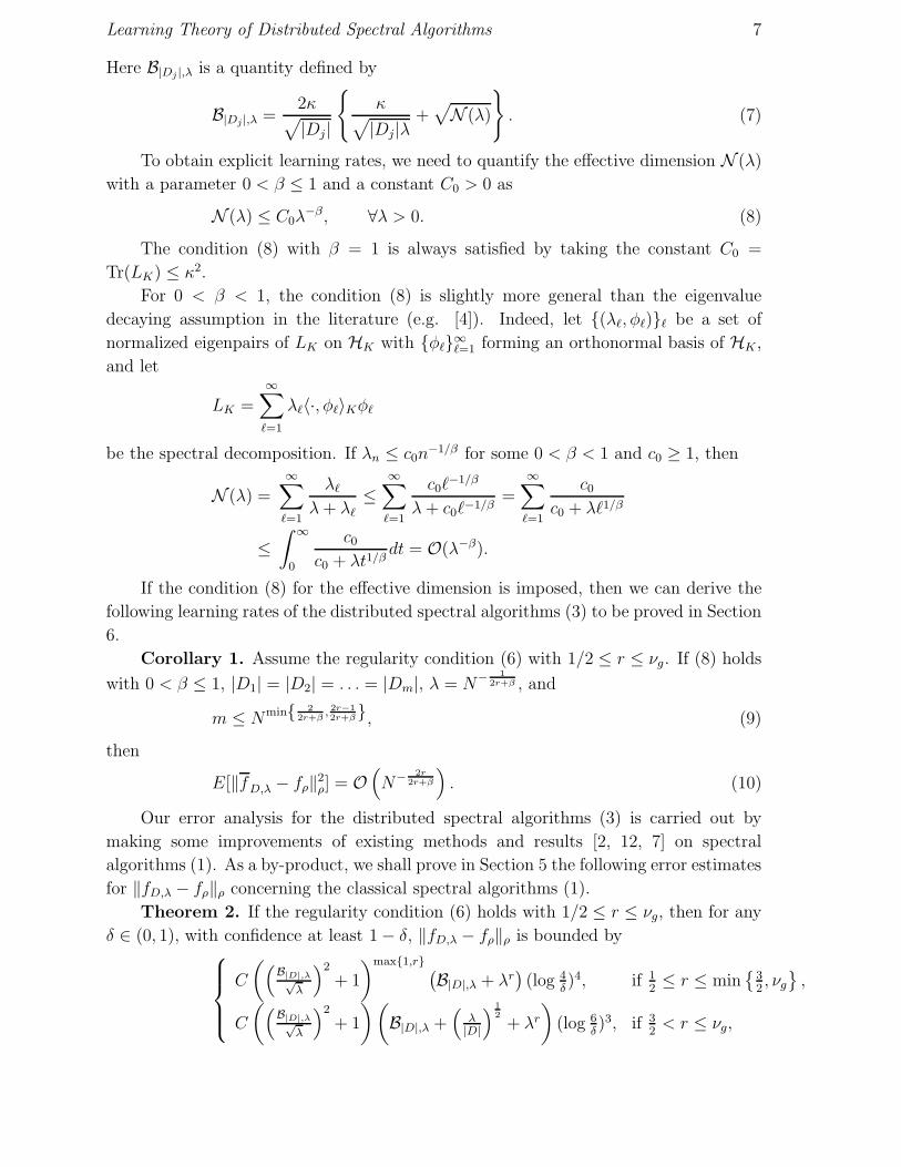
Learning Theory of Distributed Spectral Algorithms 7
Here B|Dj |,λ is a quantity defined by
B|Dj |,λ =2κ
√
|Dj|
{
κ√
|Dj|λ+√
N (λ)
}
. (7)
To obtain explicit learning rates, we need to quantify the effective dimension N (λ)
with a parameter 0 < β ≤ 1 and a constant C0 > 0 as
N (λ) ≤ C0λ−β, ∀λ > 0. (8)
The condition (8) with β = 1 is always satisfied by taking the constant C0 =
Tr(LK) ≤ κ2.
For 0 < β < 1, the condition (8) is slightly more general than the eigenvalue
decaying assumption in the literature (e.g. [4]). Indeed, let {(λℓ, φℓ)}ℓ be a set of
normalized eigenpairs of LK on HK with {φℓ}∞ℓ=1 forming an orthonormal basis of HK ,
and let
LK =∞∑
ℓ=1
λℓ〈·, φℓ〉Kφℓ
be the spectral decomposition. If λn ≤ c0n−1/β for some 0 < β < 1 and c0 ≥ 1, then
N (λ) =∞∑
ℓ=1
λℓ
λ + λℓ
≤∞∑
ℓ=1
c0ℓ−1/β
λ + c0ℓ−1/β=
∞∑
ℓ=1
c0
c0 + λℓ1/β
≤∫ ∞
0
c0
c0 + λt1/βdt = O(λ−β).
If the condition (8) for the effective dimension is imposed, then we can derive the
following learning rates of the distributed spectral algorithms (3) to be proved in Section
6.
Corollary 1. Assume the regularity condition (6) with 1/2 ≤ r ≤ νg. If (8) holds
with 0 < β ≤ 1, |D1| = |D2| = . . . = |Dm|, λ = N− 12r+β , and
m ≤ Nmin{ 22r+β
, 2r−12r+β}, (9)
then
E[‖fD,λ − fρ‖2ρ] = O
(
N− 2r2r+β
)
. (10)
Our error analysis for the distributed spectral algorithms (3) is carried out by
making some improvements of existing methods and results [2, 12, 7] on spectral
algorithms (1). As a by-product, we shall prove in Section 5 the following error estimates
for ‖fD,λ − fρ‖ρ concerning the classical spectral algorithms (1).
Theorem 2. If the regularity condition (6) holds with 1/2 ≤ r ≤ νg, then for any
δ ∈ (0, 1), with confidence at least 1 − δ, ‖fD,λ − fρ‖ρ is bounded by
C
(
(
B|D|,λ√λ
)2
+ 1
)max{1,r}(
B|D|,λ + λr)
(log 4δ)4, if 1
2≤ r ≤ min
{
32, νg
}
,
C
(
(
B|D|,λ√λ
)2
+ 1
)(
B|D|,λ +(
λ|D|
)12
+ λr
)
(log 6δ)3, if 3
2< r ≤ νg,

Learning Theory of Distributed Spectral Algorithms 8
where C is a constant independent of |D| or δ. If (8) holds with 0 < β ≤ 1 and
λ = N− 12r+β , then for any 0 < δ < 1, with confidence at least 1 − δ, we have
‖fD,λ − fρ‖ρ ≤ CN− r2r+β (log 6/δ)4 , (11)
where C is a constat independent of N or δ. Moreover,
E[
‖fD,λ − fρ‖2ρ
]
= O(
N− 2r2r+β
)
. (12)
To facilitate the use of the distributed spectral algorithms in practice, we discuss
the important issue of parameter selection by the strategy of cross-validation in two
situations.
The first situation is when the data are stored naturally across multiple servers in
a distributive way. This happens in some practical applications in medicine, finance,
business, and some other areas, and the data are not combined for reasons of protecting
privacy or avoiding high costs. In such a circumstance, the number of data subsets m is
fixed. We propose a cross-validation approach for selecting the regularization parameter
λ for the distributed spectral algorithms, as done for the regularized least squares in [5].
Without loss of generality, we assume that each data subset Dj has an even sample size
and is the disjoint union of two subsets, D1j (the training set) and D2
j (the validation
set), of equal cardinality |D1j | = |D2
j | = |Dj |/2. Let Λ be a set of positive parameters.
We use the training data subsets {D1j}m
j=1 and the distributed spectral algorithm to get
a set of estimators {fD1,λ}λ∈Λ with D1 = ∪mj=1D
1j , and then utilize the validation subsets
{D2j}m
j=1 to select an optimal parameter λ∗ by
λ∗ = arg minλ∈Λ
1
m
m∑
j=1
1
|D2j |
∑
z=(x,y)∈D2j
(
fD1,λ(x) − y)2
. (13)
The final estimator is fD1,λ∗ . Some theoretical analysis for the cross-validation strategy
can be found in [5, Theorem 3].
The other situation we consider for parameter selection in distributed learning is
when the divide-and-conquer approach is used to reduce the computational complexity
and memory requirements. Here there exist two parameters in the distributed spectral
algorithm: the number of data subsets m and the regularization parameter λ. We
assume that the data set D has size |D| = 2n for some n ∈ N. We choose
1 ≤ kmin ≤ kmax ≤ n, take m = 2k with k ∈ Kindex := {kmin, kmin + 1, . . . , kmax},and divide the data set D into m = 2k disjoint data subsets {Dj,k}2k
j=1 of size 2n−k. Here
the integer kmin is chosen according to the processing ability (for data sets of size at most
2n−kmin) of the local processors and kmax is set according to the size requirement (at
least 2n−kmax) of data subsets in the local processors. By dividing each data subset Dj,k
into the disjoint union of two subsets D1j,k and D2
j,k of equal cardinality, and applying the
distributed spectral algorithm to the training data subsets {D1j,k}m
j=1 and λ ∈ Λ, we get
a set of estimators {fD1·,k,λ}λ∈Λ with D1
·,k = ∪2k
j=1D1j,k. Then we can use the validation

Learning Theory of Distributed Spectral Algorithms 9
subsets {D2j,k}2k
j=1 to select the optimal parameter pair (k∗, λ∗) by
(k∗, λ∗) = arg min(k,λ)∈Kindex×Λ
1
2n−1
2k∑
j=1
∑
z=(x,y)∈D2j,k
(
fD1·,k,λ(x) − y
)2
. (14)
This yields the final estimator fD1·,k∗
,λ∗ . The computational cost of the above procedure
is in the order of O(
∑
λ∈Λ
∑kmax
k=kmin
(
2n−k)3)
= O(
|D|32−3kmin |Λ|)
. However, for each
choice of k, a procedure of re-partition and re-communication of the data set would be
required, which would significantly hinders the use of the proposed distributed spectral
algorithms. To the best of our knowledge, a feasible way to select m is to adjust it
manually. It is possible to select m manually via a few trails, since (9) yields optimal
rates for distributed spectral algorithms for m ≤ m0 with the largest number of data
subsets m0 depending on r and β (which is difficult to determine in practice). It would
be interesting to develop other efficient data-driven parameter selection strategies for
distributed spectral algorithms (even for the well known distributed regularized least
squares [23]) which can be rigorously justified in theory.
3. Related Work and Discussion
The study of spectral algorithms (1) has a long history in the literature of inverse
problems [8]. The generalization performance of these algorithms have been investigated
in the learning theory literature [12, 2, 5]. Let us mention some explicit results related
to this paper and demonstrate the slight improvement of our learning rates (12) for
the spectral algorithms (1) by removing a logarithmic factor from the existing results.
Note that the learning rates (12) coincide with the minimax lower bound proved in [4,
Theorem 3], and are optimal.
When the regularity condition (6) holds with 1/2 ≤ r ≤ νg, it was proved in [2,
Corollary 17] that for
N >
(
2√
2κ2 log4
δ
)4r+22r+3
, (15)
with confidence at least 1 − δ,
‖fD,λ − fρ‖ρ ≤ CN− r2r+1 log
4
δ, (16)
where C is a constant independent of δ or N . Let PN,δ be the event that (15) holds.
Then it follows from the definition of expectation that
E[‖fD,λ − fρ‖2ρ] ≤ E[‖fD,λ − fρ‖2
ρ|PN,δ] + [‖fD,λ − fρ‖2ρ|PT
N,δ], (17)
where PTN,δ denotes the event that (15) does not hold. Plugging (16) with sufficiently
small δ (δ = N−2 for example) into (17), we obtain
E[‖fD,λ − fρ‖2ρ] = O
(
N− 2r2r+1 log N
)
.
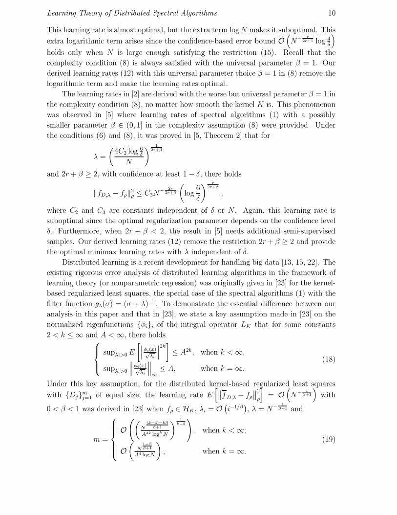
Learning Theory of Distributed Spectral Algorithms 10
This learning rate is almost optimal, but the extra term log N makes it suboptimal. This
extra logarithmic term arises since the confidence-based error bound O(
N− r2r+1 log 4
δ
)
holds only when N is large enough satisfying the restriction (15). Recall that the
complexity condition (8) is always satisfied with the universal parameter β = 1. Our
derived learning rates (12) with this universal parameter choice β = 1 in (8) remove the
logarithmic term and make the learning rates optimal.
The learning rates in [2] are derived with the worse but universal parameter β = 1 in
the complexity condition (8), no matter how smooth the kernel K is. This phenomenon
was observed in [5] where learning rates of spectral algorithms (1) with a possibly
smaller parameter β ∈ (0, 1] in the complexity assumption (8) were provided. Under
the conditions (6) and (8), it was proved in [5, Theorem 2] that for
λ =
(
4C2 log 6δ
N
)
12r+β
and 2r + β ≥ 2, with confidence at least 1 − δ, there holds
‖fD,λ − fρ‖2ρ ≤ C3N
− 2r2r+β
(
log6
δ
)r
2r+β
,
where C2 and C3 are constants independent of δ or N . Again, this learning rate is
suboptimal since the optimal regularization parameter depends on the confidence level
δ. Furthermore, when 2r + β < 2, the result in [5] needs additional semi-supervised
samples. Our derived learning rates (12) remove the restriction 2r + β ≥ 2 and provide
the optimal minimax learning rates with λ independent of δ.
Distributed learning is a recent development for handling big data [13, 15, 22]. The
existing rigorous error analysis of distributed learning algorithms in the framework of
learning theory (or nonparametric regression) was originally given in [23] for the kernel-
based regularized least squares, the special case of the spectral algorithms (1) with the
filter function gλ(σ) = (σ + λ)−1. To demonstrate the essential difference between our
analysis in this paper and that in [23], we state a key assumption made in [23] on the
normalized eigenfunctions {φi}i of the integral operator LK that for some constants
2 < k ≤ ∞ and A < ∞, there holds
supλi>0 E
[
∣
∣
∣
φi(x)√λi
∣
∣
∣
2k]
≤ A2k, when k < ∞,
supλi>0
∥
∥
∥
φi(x)√λi
∥
∥
∥
∞≤ A, when k = ∞.
(18)
Under this key assumption, for the distributed kernel-based regularized least squares
with {Dj}mj=1 of equal size, the learning rate E
[
∥
∥fD,λ − fρ
∥
∥
2
ρ
]
= O(
N− 1β+1
)
with
0 < β < 1 was derived in [23] when fρ ∈ HK , λi = O(
i−1/β)
, λ = N− 1β+1 and
m =
O(
(
N(k−4)−kβ
β+1
A4k logk N
)1
k−2
)
, when k < ∞,
O(
N1−ββ+1
A4 log N
)
, when k = ∞.
(19)
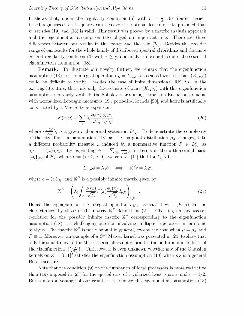
Learning Theory of Distributed Spectral Algorithms 11
It shows that, under the regularity condition (6) with r = 12, distributed kernel-
based regularized least squares can achieve the optimal learning rate provided that
m satisfies (19) and (18) is valid. This result was proved by a matrix analysis approach
and the eigenfunction assumption (18) played an important role. There are three
differences between our results in this paper and those in [23]. Besides the broader
range of our results for the whole family of distributed spectral algorithms and the more
general regularity condition (6) with r ≥ 12, our analysis does not require the essential
eigenfunction assumption (18).
Remark. To illustrate our novelty further, we remark that the eigenfunction
assumption (18) for the integral operator LK = LK,ρXassociated with the pair (K, ρX)
could be difficult to verify. Besides the case of finite dimensional RKHSs, in the
existing literature, there are only these classes of pairs (K, ρX) with this eigenfunction
assumption rigorously verified: the Sobolev reproducing kernels on Euclidean domains
with normalized Lebesgue measures [19], periodical kernels [20], and kernels artificially
constructed by a Mercer type expansion
K(x, y) =∑
i
λiφi(x)√
λi
φi(y)√λi
, (20)
where {φi(x)√λi}i is a given orthonormal system in L2
ρX. To demonstrate the complexity
of the eigenfunction assumption (18) as the marginal distribution ρX changes, take
a different probability measure µ induced by a nonnegative function P ∈ L2ρX
as
dµ = P (x)dρX . By expanding φ =∑
i∈Ici√λi
φi in terms of the orthonormal basis
{φi}i∈I of HK where I := {i : λi > 0}, we can see [11] that for λ0 > 0,
LK,µφ = λ0φ ⇐⇒ KP c = λ0c,
where c = (ci)i∈I and KP is a possibly infinite matrix given by
KP =
(
λi
∫
X
φi(x)√λi
P (x)φj(x)√
λj
dρX
)
i,j∈I
. (21)
Hence the eigenpairs of the integral operator LK,µ associated with (K, µ) can be
characterized by those of the matrix KP defined by (21). Checking an eigenvector
condition for the possibly infinite matrix KP corresponding to the eigenfunction
assumption (18) is a challenging question involving multiplier operators in harmonic
analysis. The matrix KP is not diagonal in general, except the case when µ = ρX and
P ≡ 1. Moreover, an example of a C∞ Mercer kernel was presented in [24] to show that
only the smoothness of the Mercer kernel does not guarantee the uniform boundedness of
the eigenfunctions {φi(x)√λi}i. Until now, it is even unknown whether any of the Gaussian
kernels on X = [0, 1]d satisfies the eigenfunction assumption (18) when ρX is a general
Borel measure.
Note that the condition (9) on the number m of local processors is more restrictive
than (19) imposed in [23] for the special case of regularized least squares and r = 1/2.
But a main advantage of our results is to remove the eigenfunction assumption (18)

Learning Theory of Distributed Spectral Algorithms 12
which was key in [23] to get less restrictions on m. It is a great challenge to derive
the optimal learning rates under the conditions imposed in this paper, without the
eigenfunction assumption (18), but with less demanding restriction (19) on m. Our
analysis is achieved by the novelty of using the integral operator approach and second
order decomposition of a difference of operator inverses. Similar analysis was carried out
in our recent work [11] for the special algorithm of distributed regularized least squares.
In this paper we are concerned with distributed learning with the general spectral
algorithms (1) rather than the regularized least squares. It has not been considered
in the literature, to our best knowledge. One of the advantages of distributing learning
with general spectral algorithms such as the spectral cut-off and Landweber iteration is
that the saturation of the distributed regularized least squares, stated by the restriction
r ≤ 1, is overcome and faster learning rates with r > 1 can be achieved. Corollary 1
shows that, if the number m of local machines is not too large, then the learning rates
of the distributed spectral algorithm (3) and the spectral algorithm (1) implemented on
a “big” machine with the whole data set are identical.
Comparing Corollary 1 with Theorem 2, we find the regularization parameters λ
for achieving the optimal learning rates are identical. Even though each local machine
accesses to only 1/m of the whole data, it is nonetheless essential to regularize as
we process the whole data set, which would lead to overfitting in local machines.
However, the m-fold weighted average reduces the variance and enables algorithm (3) to
achieve optimal learning rates. Though we are interested in using the general spectral
algorithms, other than the regularized least squares, mainly in the case r > 1 (at least for
overcoming the saturation) when the restriction (9), with the power exponent involving2r−12r+β
, makes more sense, it would be interesting to relax the restriction (9) by other
approaches.
After the submission of this paper in January 2016, we found that similar analysis
was independently carried out for spectral algorithms by L. H. Dicker, D. P. Foster,
and D. Hsu in a paper entitled “Kernel ridge vs. principal component regression:
minimax bounds and adaptibility of regularization operators” (arXiv:1605.08839, May
2016) and for spectral algorithms and distributed spectral algorithms by G. Blanchard
and N. Mucke in a paper entitled “Parallel spectral algorithms for kernel learning”
(arXiv:1610.07487, October 2016).
4. Second Order Decomposition for Bounding Norms
Our error analysis is based on a combination of an integral operator approach [4, 18],
a recently developed technique [11] of second order decomposition of inverse operator
differences, and a novel idea for bounding operator products developed below in this
paper. The core of the integral operator method is to analyze similarities between the
empirical integral operator LK,D and its data-free limit LK , since convergence rates
of corresponding schemes associated with LK are easier to derive. Taking spectral

Learning Theory of Distributed Spectral Algorithms 13
algorithms for example, the data-free limit of algorithms (1) is
fλ = gλ(LK)LKfρ.
According to the definition of the filter function and conditions (6), if r ≤ νg, we see
from the identity ‖f‖ρ = ‖L1/2K f‖K for f ∈ HK that
‖fλ − fρ‖ρ ≤ ‖L1/2K (gλ(LK)LK − I)L
r−1/2K ‖‖L1/2
K uρ‖K ≤ γrλr‖uρ‖ρ. (22)
The classical method to analyze similarities between LK and LK,D is to bound the
norm of operator difference LK−LK,D. We refer the readers to [2, 4, 5, 7, 10, 11, 18, 21, 9]
for details on this method. In particular, it can be found in [4, 21] and [11] that for any
δ ∈ (0, 1), with confidence at least 1 − δ, there holds
‖LK − LK,D‖ ≤ 4κ2
√
|D|log
2
δ, (23)
and
‖(λI + LK)−1/2(LK − LK,D)‖ ≤ B|D|,λ log2
δ, (24)
where B|D|,λ is defined by (7).
In our error decomposition for spectral algorithms, given in Proposition 2 below, we
use the norms of the product operators (LK+λI)(LK,D+λ)−1 and (LK,D+λI)(LK+λI)−1
which also reflect similarities between LK and LK,D, as seen from equation (26) below.
In this section, we present tight bounds of the product norms by using the second order
decomposition of operator differences. This is the first novelty of our error analysis
carried out in this paper.
Let A and B be invertible operators on a Banach space. The first order
decomposition of operator differences is
A−1 − B−1 = A−1(B − A)B−1 = B−1(B − A)A−1. (25)
It follows that
A−1B = (A−1 − B−1)B + I = A−1(B − A) + I. (26)
Let A = LK + λI and B = LK,D + λI. We see from (26) that
‖(LK + λI)−1(LK,D + λI)‖ ≤ ‖(LK + λI)−1/2‖‖(LK + λI)−1/2(LK,D − LK)‖ + 1.
Since ‖(λI + LK)−1/2‖ ≤ 1/√
λ, it follows from (24) that with confidence at least 1− δ,
there holds
‖(LK + λI)−1(LK,D + λI)‖ ≤ B|D|,λ√λ
log2
δ+ 1. (27)
To bound the norm of (LK +λI)(LK,D +λI)−1, the first order decomposition (25) is
not sufficient due to the lack of an appropriate bound for ‖(LK,D +λI)−1/2(LK,D−LK)‖.We need to decompose A−1 = A−1−B−1 +B−1 in (25) further. This is the second order
decomposition of operator difference, which was introduced in [11] to derive optimal
Learning Theory of Distributed Spectral Algorithms 14
learning rates of the regularized least squares. It asserts that if A and B are invertible
operators on a Banach space, then (25) yields
A−1 − B−1 = B−1(B − A)A−1(B − A)B−1 + B−1(B − A)B−1
= B−1(B − A)B−1(B − A)A−1 + B−1(B − A)B−1. (28)
This implies the following decomposition of the operator product
BA−1 = (B − A)B−1(B − A)A−1 + (B − A)B−1 + I. (29)
Inserting A = LK,D +λI and B = LK +λI to (29), we obtain the following upper bound
for ‖(LK + λI)(LK,D + λI)−1‖.Proposition 1. For any 0 < δ < 1, with confidence at least 1 − δ, there holds
‖(LK + λI)(LK,D + λI)−1‖ ≤ 2
[
(B|D|,λ log 2δ√
λ
)2
+ 1
]
.
Proof. We apply (29) to the operator A = LK,D +λI and B = LK +λI. Applying
the bounds ‖(λI + LK,D)−1‖ ≤ 1/λ and ‖(λI + LK)−1/2‖ ≤ 1/√
λ gives
‖(λI + LK)(λI + LK,D)−1‖ ≤ ‖(λI + LK)−1/2(LK − LK,D)‖2λ−1
+ ‖(λI + LK)−1/2(LK − LK,D)‖λ−1/2 + 1.
Here we have used the fact that
‖L1L2‖ = ‖(L1L2)T‖ = ‖LT
2 LT1 ‖ = ‖L2L1‖
for any self-adjoint operators L1, L2 on Hilbert spaces. Applying (24) yields
‖(λI + LK)(λI + LK,D)−1‖ ≤(B|D|,λ log 2
δ√λ
)2
+
(B|D|,λ log 2δ√
λ
)
+ 1
≤ 2
[
(B|D|,λ log 2δ√
λ
)2
+ 1
]
,
which proves our result. �
An upper bound of ‖(λI + LK)1/2(λI + LK,D)−1/2‖ was presented in [3], as Lemma
A.5, asserting that if
‖(LK + λI)−1/2(LK,D − LK)(LK + λI)−1/2‖ < 1 − η (30)
for some 0 < η < 1, then
‖(λI + LK)1/2(λI + LK,D)−1/2‖ ≤ 1√η.
The condition (30) with 0 < η < 1 requires the sample size N to be large enough. As
discussed in Section 3, this restriction imposes a logarithmic term in error estimates,
which makes the obtained learning rates suboptimal. We encourage the readers to
compare our Proposition 1 with Lemma A.5 of [3]. The operator product norm estimates
in Proposition 1 plays a crucial role in our integral operator approach. In particular,
based on the estimate of ‖(λI+LK)(λI+LK,D)−1‖, we present a new error decomposition
technique for spectral algorithms in the next section.
Learning Theory of Distributed Spectral Algorithms 15
5. Deriving Error Bounds for Spectral Algorithms
To analyze the spectral algorithms (1), we introduce a new error decomposition
technique, the second novelty of our error analysis. Since we do not impose any
additional Lipschitz conditions to the filter function gλ, it is not easy to bound the
difference between fD,λ and fλ. We turn to bounding the difference between fD,λ and
its semi-population version E∗[fD,λ], where
E∗[fD,λ] = E[fD,λ|x1, . . . , xN ]
denotes the conditional expectation of fD,λ given x1, . . . , xN . Since fρ = E∗[y], we then
have from (1) that
E∗[fD,λ] = gλ(LK,D)LK,Dfρ (31)
and the triangle inequality
‖fD,λ − fρ‖ρ ≤ ‖fD,λ − E∗[fD,λ]‖ρ + ‖E∗[fD,λ] − fρ‖ρ.
For the first part, since ‖L1/2K (λI + LK)−1/2‖ ≤ 1, we have
‖fD,λ − E∗(fD,λ)‖ρ =∥
∥
∥L
1/2K (fD,λ − E∗(fD,λ))
∥
∥
∥
K
≤∥
∥(λI + LK)1/2(fD,λ − E∗(fD,λ))∥
∥
K.
Denote
∆D =1
|D|∑
(x,y)∈D
(y − fρ(x))Kx. (32)
It follows from the definition of fD,λ and the property (4) of the filter function that
‖fD,λ − E∗(fD,λ)‖ρ
≤∥
∥(λI + LK)1/2(λI + LK,D)−1/2(λI + LK,D)1/2gλ(LK,D)∆D
∥
∥
K
≤ ‖(λI + LK)1/2(λI + LK,D)−1/2‖‖gλ(LK,D)(λI + LK,D)‖‖(λI + LK,D)−1/2
(λI + LK)1/2‖‖(λI + LK)−1/2∆D‖K
≤ 2b∥
∥(λI + LK)1/2(λI + LK,D)−1/2∥
∥
2 ∥∥(λI + LK)−1/2∆D
∥
∥
K.
For the second part, we have
‖E∗(fD,λ) − fρ‖ρ =∥
∥
∥L
1/2K (gλ(LK,D)LK,D − I)fρ
∥
∥
∥
K
≤∥
∥(λI + LK)1/2(gλ(LK,D)LK,D − I)fρ
∥
∥
K
≤∥
∥(λI + LK)1/2(λI + LK,D)−1/2∥
∥
∥
∥(λI + LK,D)1/2(gλ(LK,D)LK,D − I)fρ
∥
∥
K.
All the above discussion yields the following error decomposition for the spectral
algorithms.
Proposition 2. Let ∆D be defined by (32). Then we have
‖fD,λ − fρ‖ρ ≤ I1 + I2,

Learning Theory of Distributed Spectral Algorithms 16
where
I1 = 2b∥
∥(λI + LK)1/2(λI + LK,D)−1/2∥
∥
2 ∥∥(λI + LK)−1/2∆D
∥
∥
K,
I2 =∥
∥(λI + LK)1/2(λI + LK,D)−1/2∥
∥
∥
∥(λI + LK,D)1/2(gλ(LK,D)LK,D − I)fρ
∥
∥
K.
The error decomposition presented in Proposition 2 is different from that in [2]
or [5]. In fact, it can be found in Equation (26) of [2] that the difference LK − LK,D
rather than the operator product (LK +λI)(LK,D +λI)−1 is used to analyze similarities
between LK and LK,D. The error analysis in [5] needs an additional truncated function
f trλ = Pλfρ,
where Pλ is the orthogonal projector in L2ρX
defined by
Pλ = Θλ(LK),
with Θλ(σ) = 1 for σ ≥ λ and Θλ(σ) = 0 for σ < λ. Our error decomposition does not
require such a truncated function and uses the operator product to analyze similarities
between LK and LK,D.
Based on the new error decomposition technique presented in Proposition 2, we
should bound three terms:∥
∥(λI + LK)1/2(λI + LK,D)−1/2∥
∥ ,∥
∥(λI + LK)−1/2∆D
∥
∥
K, and
∥
∥(λI + LK,D)1/2(gλ(LK,D)LK,D − I)fρ
∥
∥
K. To bound the first term, we need Proposition
1 and the following lemma about norm estimates for products of powers of two positive
operators. It was proved in [1, Theorem IX.2.1-2] for positive definite matrices and then
provided in [3, Lemma A.7] for positive operators on Hilbert spaces.
Lemma 1. Let s ∈ [0, 1]. For positive operators A and B on a Hilbert space we
have
‖AsBs‖ ≤ ‖AB‖s. (33)
Applying the above lemma to A = λI + LK and B = (λI + LK,D)−1, we get from
Proposition 1 the following result.
Lemma 2. Let λ > 0, 0 ≤ s ≤ 1 and 0 < δ < 1. Then, with confidence at least
1 − δ, there holds
‖(λI + LK)s(λI + LK,D)−s‖ ≤ 2s
[
(B|D|,λ log 2δ√
λ
)2
+ 1
]s
.
The second term∥
∥(λI + LK)−1/2∆D
∥
∥
Kcan be bounded by the following lemma
found in [3] or [4].
Lemma 3. Let δ ∈ (0, 1), and D be a sample drawn independently according to
ρ. If |y| ≤ M almost surely, then with confidence at least 1 − δ, there holds
‖(λI + LK)−1/2∆D‖K ≤ 2M
κB|D|,λ log
2
δ.
To bound the third term∥
∥(λI + LK,D)1/2(gλ(LK,D)LK,D − I)fρ
∥
∥
K, we need the
following two lemmas. The first one can be found in [3, Lemma A.6], and the second
one is derived from properties (4) and (5) of the filter function gλ.

Learning Theory of Distributed Spectral Algorithms 17
Lemma 4. For positive operators A and B on a Hilbert space with ‖A‖, ‖B‖ ≤ Cfor some constant C > 0, we have for t ≥ 1,
‖At − Bt‖ ≤ tCt−1‖A − B‖. (34)
Lemma 5. For 0 < t ≤ νg, we have
‖(gλ(LK,D)LK,D − I)(λI + LK,D)t‖ ≤ 2t(b + 1 + γt)λt. (35)
Proof. Recall from the introduction that {(σx
i , φx
i )i} is a set of normalized
eigenpairs of LK,D with the eigenfunctions {φx
i }i forming an orthonormal basis of HK .
Then for each h ∈ HK , we have h =∑〈h, φx
i 〉φx
i and ‖h‖2K =
∑
i〈h, φx
i 〉2. Hence
‖(gλ(LK,D)LK,D − I)(λI + LK,D)th‖K
=
∥
∥
∥
∥
∥
∞∑
i=1
〈h, φx
i 〉(gλ(σx
i )σx
i − 1)(λ + σx
i )tφx
i
∥
∥
∥
∥
∥
K
=
{ ∞∑
i=1
[
〈h, φx
i 〉(gλ(σx
i )σx
i − 1)(λ + σx
i )t]2
}1/2
≤{ ∞∑
i=1
[
|〈h, φx
i 〉||gλ(σx
i )σx
i − 1|2t(λt + (σx
i )t)]2
}1/2
≤ 2t(b + 1 + γt)λt
{ ∞∑
i=1
(〈h, φx
i 〉)2
}1/2
= 2t(b + 1 + γt)λt‖h‖K .
The last inequalities hold due to properties (4) and (5) of the filter function gλ and the
elementary inequality (c + d)t ≤ 2t(ct + dt) for any c, d, t ≥ 0. Then our result follows
from the definition of the operator norm on HK . �
Before presenting the proof of Theorem 2, we give the following proposition.
Proposition 3. Assume (6) holds with 1/2 ≤ r ≤ νg. If 12≤ r ≤ 3/2, we have
‖fD,λ − fρ‖ρ ≤ 2bΞD‖(λI + LK)−1/2∆D‖K + 2r(b + 1 + γr)‖uρ‖ρλrΞr
D,
where
ΞD = ‖(λI + LK)(λI + LK,D)−1‖. (36)
If 32
< r ≤ νg, we have
‖fD,λ − fρ‖ρ ≤ 2bΞD‖(λI + LK)−1/2∆D‖K + Cb,r,κ‖uρ‖ρΞ1/2D (
√λ‖LK − LK,D‖ + λr),
where Cb,r,κ is a constant depending only on b, r and κ.
Proof. We estimate the two parts I1 and I2 in Proposition 2. For I1, recall the
notation ΞD = ‖(λI + LK)(λI + LK,D)−1‖ and by Lemma 1 with s = 1/2, we have
I1 ≤ 2bΞD‖(λI + LK)−1/2∆D‖K .
Now we estimate
I2 =∥
∥(λI + LK)1/2(λI + LK,D)−1/2∥
∥
∥
∥(λI + LK,D)1/2(gλ(LK,D)LK,D − I)fρ
∥
∥
K
≤ Ξ1/2D
∥
∥(λI + LK,D)1/2(gλ(LK,D)LK,D − I)fρ
∥
∥
K. (37)

Learning Theory of Distributed Spectral Algorithms 18
The regularity condition (6) with 1/2 ≤ r ≤ νg means fρ = LrKuρ for some uρ ∈ L2
ρX.
To estimate the term∥
∥(λI + LK,D)1/2(gλ(LK,D)LK,D − I)fρ
∥
∥
K, we consider two cases
according to different regularity levels as follows.
Case 1: If r ∈ [1/2, 3/2], we have∥
∥(λI + LK,D)1/2(gλ(LK,D)LK,D − I)fρ
∥
∥
K
=∥
∥
∥(λI + LK,D)1/2(gλ(LK,D)LK,D − I)L
r−1/2K L
1/2K uρ
∥
∥
∥
K
= ‖(λI + LK,D)1/2(gλ(LK,D)LK,D − I)(λI + LK,D)r−1/2(λI + LK,D)−(r−1/2)
(λI + LK)r−1/2(λI + LK)−(r−1/2)Lr−1/2K L
1/2K uρ‖K
≤ ‖(gλ(LK,D)LK,D − I)(λI + LK,D)r‖Ξr−1/2D ‖uρ‖ρ,
where the last inequality follows from Lemma 1 with s = r−1/2 ∈ [0, 1], and the bound
‖(λI + LK)−(r−1/2)Lr−1/2K ‖ ≤ 1. Thus,
I2 ≤ ‖(gλ(LK,D)LK,D − I)(λI + LK,D)r‖ΞrD‖uρ‖ρ.
Combining the above estimates and Lemma 5 with t = r yields
I2 ≤ 2r(b + 1 + γr)‖uρ‖ρλrΞr
D. (38)
Case 2: If r > 3/2, we decompose∥
∥(λI + LK,D)1/2(gλ(LK,D)LK,D − I)fρ
∥
∥
Kas
‖(λI + LK,D)1/2(gλ(LK,D)LK,D − I)fρ‖K
= ‖(λI + LK,D)1/2(gλ(LK,D)LK,D − I)(LK)r−1/2L1/2K uρ‖K
≤ ‖(λI + LK,D)1/2(gλ(LK,D)LK,D − I)(LK)r−1/2‖‖uρ‖ρ. (39)
By adding and subtracting the operator (LK,D)r−1/2, we can continue the estimation as
‖(λI + LK,D)1/2(gλ(LK,D)LK,D − I)(LK)r−1/2‖≤ ‖(λI + LK,D)1/2(gλ(LK,D)LK,D − I)((LK)r−1/2 − (LK,D)r−1/2)‖+‖(λI + LK,D)1/2(gλ(LK,D)LK,D − I)(LK,D)r−1/2‖.
Since r > 3/2, applying Lemma 4 to A = LK and B = LK,D with t = r − 1/2 > 1, we
have
‖(LK)r−1/2 − (LK,D)r−1/2‖ ≤ (r − 1/2)κ2r−3‖LK − LK,D‖.Combining this observation with the bound ‖(λI + LK,D)r−1/2(LK,D)r−1/2‖ ≤ 1, and
applying Lemma 5 with t = 1/2 or t = r, we know that
‖(λI + LK,D)1/2(gλ(LK,D)LK,D − I)(LK)r−1/2‖≤ ‖(λI + LK,D)1/2 (gλ(LK,D)LK,D − I) ‖(r − 1/2)κ2r−3‖LK − LK,D‖
+ ‖(gλ(LK,D)LK,D − I)(λI + LK,D)r‖≤ (b + 1 + γ 1
2)(r − 1/2)κ2r−3
√λ‖LK − LK,D‖ + 2r(b + 1 + γr)λ
r
≤ Cb,r,κ(√
λ‖LK − LK,D‖ + λr),
where Cb,r,κ = (b + 1 + γ 12)(r − 1/2)κ2r−3 + 2r(b + 1 + γr). Putting the above estimates
into inequality (39) yields our desired error bound. �
Learning Theory of Distributed Spectral Algorithms 19
Now we are in a position to prove Theorem 2.
Proof of Theorem 2. By Proposition 1, for δ ∈ (0, 1), there exists a subset Z |D|δ,1
of Z |D| of measure at least 1 − δ such that
ΞD = ‖(λI + LK)(λI + LK,D)−1‖ ≤ 2
[
(B|D|,λ log 2δ√
λ
)2
+ 1
]
, ∀D ∈ Z |D|δ,1 .
By Lemma 3 there exists another subset Z |D|δ,2 of Z |D| of measure at least 1− δ such that
‖(λI + LK)−1/2∆D‖K ≤ 2M
κB|D|,λ log
2
δ, ∀D ∈ Z |D|
δ,2 .
According to (23), there exists a third subset Z |D|δ,3 of Z |D| of measure at least 1− δ such
that
‖LK − LK,D‖ ≤ 4κ2 log 2δ
√
|D|, ∀D ∈ Z |D|
δ,3 .
Put the above observations into Proposition 3. When r ∈ [12, 3
2], we know that for
D ∈ Z |D|δ,1
⋂Z |D|δ,2 , there holds
‖fD,λ − fρ‖ρ ≤ 8Mbκ
[
(
B|D|,λ log 2δ√
λ
)2
+ 1
]
B|D|,λ log 2δ
+4r(b + 1 + γr)‖uρ‖ρλr
[
(
B|D|,λ log 2δ√
λ
)2
+ 1
]r
≤ C
[
(
B|D|,λ log 2δ√
λ
)2
+ 1
]max{1,r}(
B|D|,λ log 2δ
+ λr)
,
where C = 8Mbκ
+4r(b+1+ γr)‖uρ‖ρ. Then our first desired bound is verified by scaling
2δ to δ.
When r > 32, for D ∈ Z |D|
δ,1
⋂Z |D|δ,2
⋂Z |D|δ,3 , there holds
‖fD,λ − fρ‖ρ ≤8Mb
κ
[
(B|D|,λ log 2δ√
λ
)2
+ 1
]
B|D|,λ log2
δ
+√
2Cb,r,κ‖uρ‖ρ
[
(B|D|,λ log 2δ√
λ
)2
+ 1
]12[
4κ2
(
λ
|D|
)12
log2
δ+ λr
]
≤ C
[
(B|D|,λ log 2δ√
λ
)2
+ 1
][
B|D|,λ log2
δ+
(
λ
|D|
)12
log2
δ+ λr
]
,
where C = 8Mbκ
+√
2Cb,r,κ‖uρ‖ρ(4κ2 + 1). Then we get our first desired bound for
‖fD,λ − fρ‖ρ by scaling 3δ to δ.
To prove the second desired bound, we notice from the condition N (λ) ≤ C0λ−β,
and the choices 1/2 ≤ r ≤ νg and λ = N− 12r+β that B|D|,λ can be bounded as
B|D|,λ =2κ√N
{
κ√Nλ
+√
N (λ)
}
≤ 2(κ2 + κ√
C0)N− r
2r+β ,
and(B|D|,λ√
λ
)2
+ 1 ≤ 4(
κ2 + κ√
C0
)2
+ 1.

Learning Theory of Distributed Spectral Algorithms 20
Putting the above observations into our first proved bound, we know that when
r ∈ [12, 3
2], with confidence at least 1 − δ, ‖fD,λ − fρ‖ρ is bounded by
C
[
4(
κ2 + κ√
C0
)2
+ 1
]max{1,r}(2κ2 + 2κ
√
C0 + 1)N− r2r+β (log
4
δ)4
= CN− r2r+β (log
4
δ)4,
where C = C[
4(
κ2 + κ√
C0
)2+ 1]max{1,r}
(2κ2 + 2κ√
C0 + 1).
When r > 32, with confidence at least 1 − δ, ‖fD,λ − fρ‖ρ is bounded by
C
[
4(
κ2 + κ√
C0
)2
+ 1
]
[
(2κ2 + 2κ√
C0 + 1)N− r2r+β + N− 2r+β+1
2(2r+β)
]
(log6
δ)3
≤ CN− r2r+β (log
6
δ)3,
where C = 2C[
4(
κ2 + κ√
C0
)2+ 1]
(
κ2 + κ√
C0 + 2)
. This proves our second desired
bound (11) for ‖fD,λ − fρ‖ρ.
Finally, we apply the formula
E[ξ] =
∫ ∞
0
Prob[ξ > t]dt (40)
for nonnegative random variables to ξ = ‖fD,λ − fρ‖2ρ and use the bound
Prob [ξ > t] = Prob[
ξ12 > t
12
]
≤ 6 exp{
−C− 14 N
r8r+4β t
18
}
derived from (11) for t > C log 64N− r2r+β . Then
E[
‖fD,λ − fρ‖2ρ
]
≤ C2 log 68N− 2r2r+β + 6
∫ ∞
0
exp{
−C− 14 N
r8r+4β t
18
}
dt.
The second term equals 48C2N− 2r2r+β
∫∞0
u8−1 exp {−u} du. Due to∫∞0
ud−1 exp {−u} du =
Γ(d) for d > 0, we have
E[‖fD,λ − fρ‖2ρ] ≤ (6Γ(9) + log 68)C2N− 2r
2r+β .
This completes the proof of Theorem 2. �
6. Proving Main Results for Distributed Algorithms
To present the proof, we need an error decomposition for the distributed spectral
algorithms (3).
Proposition 4. Let fD,λ be defined by (3). We have
E[‖fD,λ−fρ‖2ρ] ≤
m∑
j=1
|Dj|2|D|2 E
[
‖fDj ,λ − fρ‖2ρ
]
+m∑
j=1
|Dj ||D|
∥
∥E[fDj ,λ] − fρ
∥
∥
2
ρ.(41)

Learning Theory of Distributed Spectral Algorithms 21
Proof. Due to (3) and∑m
j=1|Dj ||D| = 1, we have
‖fD,λ − fρ‖2ρ =
∥
∥
∥
∥
∥
m∑
j=1
|Dj||D| (fDj ,λ − fρ)
∥
∥
∥
∥
∥
2
ρ
=m∑
j=1
|Dj|2|D|2 ‖fDj ,λ − fρ‖2
ρ +m∑
j=1
|Dj ||D|
⟨
fDj ,λ − fρ,∑
k 6=j
|Dk||D| (fDk,λ − fρ)
⟩
ρ
.
Taking expectations gives
E[
‖fD,λ − fρ‖2ρ
]
=
m∑
j=1
|Dj|2|D|2 E
[
‖fDj ,λ − fρ‖2ρ
]
+
m∑
j=1
|Dj||D|
⟨
EDj[fDj ,λ] − fρ, E[fD,λ] − fρ −
|Dj||D|
(
EDj[fDj ,λ] − fρ
)
⟩
ρ
.
Butm∑
j=1
|Dj||D|
⟨
EDj[fDj ,λ] − fρ, E[fD,λ] − fρ
⟩
ρ= E
[
⟨
fD,λ − fρ, E[fD,λ] − fρ
⟩
ρ
]
=∥
∥E[fD,λ] − fρ
∥
∥
2
ρ.
So we know that E[
‖fD,λ − fρ‖2ρ
]
equalsm∑
j=1
|Dj|2|D|2 E
[
‖fDj ,λ − fρ‖2ρ
]
−m∑
j=1
|Dj|2|D|2
∥
∥E[fDj ,λ] − fρ
∥
∥
2
ρ+∥
∥E[fD,λ] − fρ
∥
∥
2
ρ.
Furthermore, by the Schwartz inequality and∑m
j=1|Dj ||D| = 1, we have
‖E[fD,λ]−fρ‖2ρ =
∥
∥
∥
∥
∥
m∑
j=1
|Dj ||D|
(
E[fDj ,λ] − fρ
)
∥
∥
∥
∥
∥
2
ρ
≤m∑
j=1
|Dj||D|
∥
∥E[fDj ,λ] − fρ
∥
∥
2
ρ.(42)
Then the desired bound follows. �
The estimate (42) for the general distributed spectral algorithms is worse than
that for the distributed regularized least squares presented in [23, 11], which leads to
the restriction (9) on the number m of local processors. It would be interesting to
improve this estimate, at least for some families of spectral algorithms by imposing
some conditions on the filter function gλ.
By using Proposition 4, we can now prove Theorem 1.
Proof of Theorem 1. We apply the bound (41) in Proposition 4.
The proof in the case 12≤ r ≤ 3
2is easy. We apply Theorem 2 to the data set Dj
with an arbitrarily fixed j = 1, 2, . . . , m, and with confidence at least 1 − δ,
‖fDj ,λ − fρ‖ρ ≤ C
[
(B|Dj |,λ√λ
)2
+ 1
]max{1,r}(
B|Dj |,λ + λr)
(
log4
δ
)4
.
Using (40), it is easy to derive
E[
‖fDj ,λ − fρ‖2ρ
]
≤ 4Γ(9)C2
[
(B|Dj |,λ√λ
)2
+ 1
]max{2,2r}(
B|Dj |,λ + λr)2
.
Learning Theory of Distributed Spectral Algorithms 22
Then the first term in bound (41) can be estimated asm∑
j=1
|Dj|2|D|2 E
[
‖fDj ,λ − fρ‖2ρ
]
≤ 4Γ(9)C2
m∑
j=1
|Dj |2|D|2
[
(B|Dj |,λ√λ
)2
+ 1
]max{2,2r}(
B|Dj |,λ + λr)2
. (43)
We turn to estimate the second term of (41). For each fixed j ∈ {1, 2, . . . , m}, by
Jensen’s inequality, we have
‖E[fDj ,λ] − fρ‖ρ ≤ E[‖E∗[fDj ,λ] − fρ‖ρ].
The proof of Proposition 2 and the bounds (37) and (38) tell us that
‖E∗[fDj ,λ] − fρ‖ρ ≤ 2r(b + 1 + γr)‖uρ‖ρλrΞr
Dj.
It follows that
‖E[fDj ,λ] − fρ‖ρ ≤ 2r(b + 1 + γr)‖uρ‖ρλrE[
ΞrDj
]
. (44)
Applying Proposition 1 to each fixed j ∈ {1, . . . , m}, with confidence at least 1 − δ,
there holds
ΞDj≤ 2
[
(B|Dj |,λ log 2δ√
λ
)2
+ 1
]
.
Use the expectation formula (40) for the nonnegative random variable ξ = ΞrDj
and
Prob[ξ > t] = Prob[ξ1r > t
1r ] ≤ 2 exp
(
− λ1/2t12r√
2(B2|Dj |,λ + λ)1/2
)
.
We find
E[
ΞrDj
]
≤ 2
∫ ∞
0
exp
(
− λ1/2t12r√
2(B2|Dj |,λ + λ)1/2
)
dt,
which equals
4r2r
[
(B|Dj |,λ√λ
)2
+ 1
]r∫ ∞
0
u2r−1 exp {−u} du.
Due to∫∞0
u2r−1 exp {−u} du = Γ(2r) we have
E[
ΞrDj
]
≤ rΓ(2r)2r+2
[
(B|Dj |,λ√λ
)2
+ 1
]r
.
Inserting the above estimate to (44), we have
‖E[fDj ,λ]−fρ‖ρ ≤ rΓ(2r)22r+2(b+1+γr)‖uρ‖ρλr
[
(B|Dj |,λ√λ
)2
+ 1
]r
.(45)
Learning Theory of Distributed Spectral Algorithms 23
Combining (41), (43) and (45) we have
E[‖fD,λ − fρ‖2ρ] ≤ 4Γ(9)C2
m∑
j=1
|Dj|2|D|2
[
(B|Dj |,λ√λ
)2
+ 1
]max{2,2r}(
B|Dj |,λ + λr)2
+ r2Γ2(2r)(b + 1 + γr)224r+4‖uρ‖2
ρλ2r
m∑
j=1
|Dj||D|
[
(B|Dj |,λ√λ
)2
+ 1
]2r
.
This proves the desired bound in the case 1/2 ≤ r ≤ 3/2.
The proof in the case r > 3/2 is more involved. Again we first use Theorem 2 to
bound E[‖fDj ,λ − fρ‖2ρ] and obtain
m∑
j=1
|Dj|2|D|2 E
[
‖fDj ,λ − fρ‖2ρ
]
≤ 6Γ(7)C2m∑
j=1
|Dj |2|D|2
[
(B|Dj |,λ√λ
)2
+ 1
]2 [
B|Dj |,λ +
(
λ
|Dj|
)12
+ λr
]2
. (46)
Then we estimate
‖E[fDj ,λ] − fρ‖ρ ≤ E‖E∗[fDj ,λ] − fρ‖ρ
for each fixed j as in the proof of Proposition 3 to have
‖E∗[fDj ,λ] − fρ‖ρ ≤ Ξ12Dj
∥
∥
∥(λI + LK,Dj
)12 (gλ(LK,Dj
)LK,Dj− I)L
r− 12
K
∥
∥
∥‖uρ‖ρ
≤ Ξ12Dj‖(gλ(LK,Dj
)LK,Dj− I)(LK,Dj
+ λI)r‖‖uρ‖ρ + Ξ12Dj‖uρ‖ρ
‖(LK,Dj+ λI)1/2(gλ(LK,Dj
)LK,Dj− I)((LK,Dj
+ λI)r− 12 − (LK + λI)r− 1
2 )‖=: B1,Dj
+ B2,Dj.
The first term B1,Djabove can be estimated easily from Proposition 1 and Lemma 5:
with confidence at least 1 − δ, there holds
B1,Dj≤ 2r+1/2
[
(B|Dj |,λ log 2δ√
λ
)2
+ 1
]1/2
‖uρ‖ρ(b + 1 + γr)λr. (47)
The most technical part of the proof is to estimate the second term B2,Djabove.
We shall do so in two different cases on the following operator decomposition
(LK,Dj+ λI)r−1/2 − (LK + λI)r−1/2
= (LK,Dj+ λI)
(
(LK,Dj+ λI)r−3/2 − (LK,Dj
+ λI)−1(LK + λI)r−1/2)
= (LK,Dj+ λI)
(
((LK,Dj+ λI)r−3/2 − (LK + λI)r−3/2)
+ ((LK + λI)−1 − (LK,Dj+ λI)−1)(LK + λI)r−1/2
)
.
Case 1: 3/2 < r ≤ 5/2. In this case 0 < r − 3/2 ≤ 1. Then,
(LK,Dj+ λI)r−3/2 − (LK + λI)r−3/2
= (LK,Dj+ λI)r−3/2
(
I − (LK,Dj+ λI)−(r−3/2)(LK + λI)r−3/2
)

Learning Theory of Distributed Spectral Algorithms 24
and
((LK + λI)−1 − (LK,Dj+ λI)−1)(LK + λI)r−1/2
= (LK + λI)−1(LK,Dj− LK)(LK,Dj
+ λI)−1(LK + λI)r−1/2.
Thus we have
B2,Dj≤ Ξ
1/2Dj
‖uρ‖ρ
∥
∥(LK,Dj+ λI)1/2(gλ(LK,Dj
)LK,Dj− I)(LK,Dj
+ λI)
·(
(LK,Dj+ λI)r−3/2
(
I − (LK,Dj+ λI)−(r−3/2)(LK + λI)r−3/2
)
+ (LK + λI)−1(LK,Dj− LK)(LK,Dj
+ λI)−1(LK + λI)r−1/2)∥
∥
≤ Ξ1/2Dj
‖uρ‖ρ
∥
∥(gλ(LK,Dj)LK,Dj
− I)(LK,Dj+ λI)r
∥
∥
·(
1 +∥
∥(LK,Dj+ λI)−(r−3/2)(LK + λI)r−3/2
∥
∥
)
+ Ξ1/2Dj
‖uρ‖ρ
∥
∥(gλ(LK,Dj)LK,Dj
− I)(LK,Dj+ λI)3/2
∥
∥
· 1√λ
∥
∥(LK + λI)−1/2(LK,Dj− LK)
∥
∥ΞDj
∥
∥(LK + λI)r−3/2∥
∥ .
Since 0 < r − 3/2 ≤ 1, we have from (33) that∥
∥(LK,Dj+ λI)−(r−3/2)(LK + λI)r−3/2
∥
∥ ≤ Ξr−3/2Dj
.
It follows from (24), Lemma 5, and ‖LK‖ ≤ κ2 that there exists a subset Z|Dj |δ,1 of Z |Dj |
with measure 1 − δ such that for Dj ∈ Z |Dj |δ,1 ,
B2,Dj≤ Ξ
1/2Dj
‖uρ‖ρ2r(b + 1 + γr)λ
r(1 + Ξr−3/2Dj
)
+ (2κ)3Ξ3/2Dj
‖uρ‖ρ(b + 1 + γ3/2)λB|Dj |,λ log2
δ.
According to Proposition 1, there exists a subset Z |Dj |δ,2 of Z |Dj |
δ,1 with measure 1 − 2δ
such that for Dj ∈ Z |Dj |δ,2 ,
B2,Dj≤ 4r‖uρ‖ρ
[
(B|Dj |,λ log 2δ√
λ
)2
+ 1
]r−1
(b + 1 + γr)λr
+ (2κ)3√
2
[
(B|Dj |,λ log 2δ√
λ
)2
+ 1
]3/2
‖uρ‖ρ(b + 1 + γ3/2)λB|Dj |,λ log2
δ
≤ ‖uρ‖ρ
[
(B|Dj |,λ log 2δ√
λ
)2
+ 1
]3/2
×[
4r(b + 1 + γr)λr + (2κ)3
√2(b + 1 + γ3/2)λB|Dj |,λ log
2
δ
]
.
This together with (47) tells us that with confidence at least 1 − δ, ‖E∗[fDj ,λ] − fρ‖ρ is
bounded by
2r+1/2
[
(B|D|,λ log 4δ√
λ
)2
+ 1
]1/2
‖uρ‖ρ(b + 1 + γr)λr
Learning Theory of Distributed Spectral Algorithms 25
+ ‖uρ‖ρ
[
(B|Dj |,λ log 4δ√
λ
)2
+ 1
]3/2
×[
4r(b + 1 + γr)λr + (2κ)3
√2(b + 1 + γ3/2)λB|Dj |,λ log
4
δ
]
≤ C ′
[
(B|Dj |,λ√λ
)2
+ 1
]3/2[
λr + λB|Dj |,λ]
(
log4
δ
)4
,
where
C ′ = ‖uρ‖ρ max{(2r+1/2 + 4r)(b + 1 + γr), (2κ)3√
2(b + 1 + γ3/2)}. (48)
Then, using the formula (40), we have
E[‖E∗[fDj ,λ] − fρ‖ρ] ≤ 4C ′Γ(5)
[
(B|Dj |,λ√λ
)2
+ 1
]3/2[
λr + λB|Dj |,λ]
.
This means
‖E[fDj ,λ] − fρ‖2ρ ≤ (4C ′Γ(5))2
[
(B|Dj |,λ√λ
)2
+ 1
]3[
λr + λB|Dj |,λ]2
.
The above estimate together with (46) and (41) yields
E[‖fD,λ − fρ‖2ρ] ≤ 6Γ(7)C2
m∑
j=1
|Dj|2|D|2
[
(B|Dj |,λ√λ
)2
+ 1
]2 [
B|Dj |,λ +
(
λ
|Dj|
)12
+ λr
]2
+ (4C ′Γ(5))2m∑
j=1
|Dj||D|
[
(B|Dj |,λ√λ
)2
+ 1
]3[
λr + λB|Dj |,λ]2
.
This verifies the desired bound in the case 32
< r ≤ 52.
Case 2: r > 5/2. In this case, we do not need to apply Lemma 2 to control the
norm of a product operator. Instead, we can apply Lemma 4 directly (but lose the
advantage of a tighter index r) to get
B2,Dj≤ Ξ
1/2Dj
‖uρ‖ρ
∥
∥(LK,Dj+ λI)1/2(gλ(LK,Dj
)LK,Dj− I)(LK,Dj
+ λI)
·(
((LK,Dj+ λI)r−3/2 − (LK + λI)r−3/2)
+ (LK + λI)−1(LK,Dj− LK)(LK,Dj
+ λI)−1(LK + λI)r−1/2)∥
∥ .
It follows from Lemma 5 that
B2,Dj≤ 23/2(b + 1 + γ3/2)λ
3/2Ξ1/2Dj
‖uρ‖ρ
·(
(r − 3/2)κ2r−5‖LK,Dj− LK‖ + ΞDj
(2κ)2r−3
√λ
‖(LK + λI)−1/2(LK,Dj− LK)‖
)
.
From Proposition 1, (23) and (24), with confidence at least 1 − δ, there holds
B2,Dj≤ 4(b + 1 + γ3/2)λ
3/2
[
(B|Dj |,λ log 6δ√
λ
)2
+ 1
]1/2
‖uρ‖ρ
·(
(r − 3/2)κ2r−54κ2 log 6/δ√
|Dj|+ 2
[
(B|Dj |,λ log 6δ√
λ
)2
+ 1
]
(2κ)2r−3
√λ
B|Dj |,λ log6
δ
)
.

Learning Theory of Distributed Spectral Algorithms 26
Combining the above estimate with (47), we obtain, with confidence 1 − δ,
‖E∗[fDj ,λ] − fρ‖ρ ≤ 2r+1/2
[
(B|Dj |,λ log 6δ√
λ
)2
+ 1
]1/2
‖uρ‖ρ(b + 1 + γr)λr
+ 4(b + 1 + γ3/2)λ3/2
[
(B|Dj |,λ log 6δ√
λ
)2
+ 1
]1/2
‖uρ‖ρ
·(
(r − 3/2)κ2r−54κ2 log 6/δ√
|Dj|+ 2
[
(B|Dj |,λ log 6δ√
λ
)2
+ 1
]
(2κ)2r−3
√λ
B|Dj |,λ log6
δ
)
≤ C ′′
[
(B|Dj |,λ√λ
)2
+ 1
]3/2(
λr + λ3/2 1√
|Dj|+ λB|Dj |,λ
)
(
log6
δ
)4
,
where
C ′′ = ‖uρ‖ρ max{2r+1/2(b + 1 + γr), 4(b + 1 + γ3/2)(γ − 3/2)κ2r−5, 8(2b + γ3/2)(2κ)2r−3}.
By (40), we have
E[‖E∗[fDj ,λ] − fρ‖ρ] ≤ C ′′6Γ(5)
[
(B|Dj |,λ√λ
)2
+ 1
]3/2(
λr + λ3/2 1√
|Dj|+ λB|Dj |,λ
)
.
Hence
‖E[fDj ,λ] − fρ‖2ρ ≤ (C ′′6Γ(5))2
[
(B|Dj |,λ√λ
)2
+ 1
]3(
λr + λ3/2 1√
|Dj|+ λB|Dj |,λ
)2
.
The above estimate, together with (46) and (41), tells us that E[‖fD,λ−fρ‖2ρ] is bounded
by
6Γ(7)C2m∑
j=1
|Dj|2|D|2
[
(B|Dj |,λ√λ
)2
+ 1
]2 [
B|Dj |,λ +
(
λ
|Dj |
)12
+ λr
]2
+ (C ′′6Γ(5))2m∑
j=1
|Dj||D|
[
(B|Dj |,λ√λ
)2
+ 1
]3(
λr + λ3/2 1√
|Dj|+ λB|Dj |,λ
)2
.
This proves the desired bound in the case of r > 5/2. The proof of Theorem 1 is
complete. �
Proof of Corollary 1. Putting the choice λ = N−1/(2r+β) into condition (8)
yields N (λ) ≤ C0Nβ/(2r+β). For 1/2 ≤ r ≤ 3/2, since m ≤ N (2r−1)/(2r+β) and
|D1| = |D2| = . . . = |Dm|, we have
N (λ)
λ|Dj|≤ C0mN
1−2r2r+β ≤ C0.
We also have, for each j = 1, . . . , m,
B|Dj |,λ√λ
=2κ
√
λ|Dj |
{
κ√
|Dj|λ+√
N (λ)
}
≤ 2κ(κ +√
C0)
Learning Theory of Distributed Spectral Algorithms 27
and
|Dj||D| B
2|Dj |,λ ≤ 4κ2
|D|
{
κ√
|Dj|λ+√
N (λ)
}2
≤ 4κ2(κ +√
C0)2N−2r/(2r+β).
Then by Theorem 1,
E[‖fD,λ − fρ‖2ρ] ≤ C
1
m
m∑
j=1
(4κ2(κ +√
C0)2)3(4κ2(κ +
√
C0)2 + 1)N− 2r
2r+β
= CN− 2r2r+β ,
where
C = C(4κ2(κ +√
C0)2)3(4κ2(κ +
√
C0)2 + 1).
For r > 3/2, since m ≤ N2/(2r+β), we have
|Dj||D| B
2|Dj |,λ ≤ 4κ2(κ +
√
C0)2N−2r/(2r+β),
and
λ2B2|Dj |,λ ≤ 4κ2(κ +
√
C0)2N−2r/(2r+β).
So by Theorem 1, we have
E[‖fD,λ − fρ‖2ρ] ≤ C
1
m
m∑
j=1
(4κ2(κ +√
C0)2 + 1)3(8κ2(κ +
√
C0)2 + 3)N− 2r
2r+β
= C ′N− 2r2r+β ,
where
C ′ = C(4κ2(κ +√
C0)2 + 1)3(8κ2(κ +
√
C0)2 + 3).
This completes the proof of Corollary 1. �
Acknowledgement
The work described in this paper is partially supported by the NSFC/RGC Joint
Research Scheme [RGC Project No. N CityU120/14 and NSFC Project No.
11461161006] and by the National Natural Science Foundation of China [Grant No.
11401524, No. 11531013, No. 61502342, and No. 11471292]. The corresponding author
is Shao-Bo Lin.
References
[1] R. Bathis, Matrix Analysis, Volume 169 of Graduate Texts in Mathematics. Springer, 1997.
[2] F. Bauer, S. Pereverzev, L. Rosasco, On regularziation algorithms in learning theory, J. Complex.
23 (2007), 52-72.
[3] G. Blanchard, N. Kramer, Optimal learning rates for kernel conjugate gradient regression, NIPs
2010: 226-234.

Learning Theory of Distributed Spectral Algorithms 28
[4] A. Caponnetto, E. DeVito, Optimal rates for the regularized least squares algorithm, Found.
Comp. Math., 7 (2007), 331-368.
[5] A. Caponnetto, Y. Yao, Cross-validation based adaptation for regularization operators in learning
theory, Anal. Appl., 8 (2010), 161-183.
[6] F. Cucker, D. X. Zhou, Learning Theory: An Approximation Theory Viewpoint, Cambridge
University Press, Cambridge, 2007.
[7] E. De Vito, L. Rosasco, A. Caponnetto, U. De Giovannini, F. Odone, Learning from examples as
an inverse problem, J. Machine Learning Research, 6 (2005), 883-904.
[8] H. W. Engl, M. Hanke, A. Neubauer, Regularization of inverse problems. Vol. 375 of Mathematics
and Its Applications, Kluwer Academic Publishers, 1996. Group, Dordrecht.
[9] D. Hsu, S. M. Kakade, T. Zhang, Random design analysis of ridge regression, Found. Comput.
Math., 14 (2014), 569-600.
[10] T. Hu, J. Fan, Q. Wu, D. X. Zhou, Regularization schemes for minimum error entropy principle,
Anal. Appl., 13 (2015), 437-455.
[11] S. Lin, X. Guo, D. X. Zhou, Distributed learning with least square regularization, J. Mach. Learn.
Res., Submitted in 2015, revised version submitted in 2016, under review, (arXiv 1608.03339),
2016.
[12] L. Lo Gerfo, L. Rosasco, F. Odone, E. De Vito, A. Verri. Spectral algorithms for supervised
learning, Neural Comput., 20 (2008), 1873-1897.
[13] G. Mann, R. McDonald, M. Mohri, N. Silberman, D. Walker, Efficient large-scale distributed
training of conditional maximum entropy models, In NIPS, 2009.
[14] R. Tyrrell Rockafellar, Matrix Analysis, Princeton University Press, 1997.
[15] O. Shamir N. Srebro, Distributed stochastic optimization and learning, In 52nd Annual Allerton
Conference on Communication, Control and Computing, 2014.
[16] S. Smale, D. X. Zhou, Shannon sampling and function reconstruction from point values, Bull.
Amer. Math. Soc., 41 (2004), 279-305.
[17] S. Smale, D. X. Zhou, Shannon sampling II: Connections to learning theory, Appl. Comput.
Harmonic Anal., 19 (2005), 285-302.
[18] S. Smale, D. X. Zhou, Learning theory estimates via integral operators and their approximations,
Constr. Approx., 26 (2007), 153-172.
[19] I. Steinwart, D. Hush, C. Scovel, Optimal rates for regularized least squares regression, in
Proceedings of the 22nd Annual Conference on Learning Theory (S. Dasgupta and A. Klivans,
eds.), pp. 79-93, 2009.
[20] R. C. Williamson, A. J. Smola, B. Scholkopf, Generalization performance of regularization
networks and support vector machines via entropy numbers of compact operators, IEEE Trans.
Inform. Theory, 47 (2001), 2516-2532.
[21] Y. Yao, L. Rosasco, A. Caponnetto, On early stopping in gradient descent learning, Constr.
Approx., 26 (2007), 289-315.
[22] Y. C. Zhang, J. Duchi, M. Wainwright, Communication-efficient algorithms for statistical
optimization, J. Mach. Learn. Res., 14 (2013), 3321-3363.
[23] Y. C. Zhang, J. Duchi, M. Wainwright, Divide and conquer kernel ridge regression: A distributed
algorithm with minimax optimal rates, J. Mach. Learn. Res., 16(2015), 3299-3340.
[24] D. X. Zhou, The covering number in learning theory, J. Complex., 18 (2002), 739–767.