Journal of Machine Learning Research 7 (2006) 665–704 Submitted 9/05; Published 4/06

Learning Minimum Volume Sets

Clayton D. Scott CSCOTT@RICE.EDU

Department of StatisticsRice UniversityHouston, TX 77005, USA

Robert D. Nowak NOWAK@ECE.WISC.EDU

Department of Electrical and Computer EngineeringUniversity of Wisconsin at MadisonMadison, WI 53706, USA

Editor: John Lafferty

AbstractGiven a probability measureP and a reference measureµ, one is often interested in the minimumµ-measure set withP-measure at leastα. Minimum volume sets of this type summarize the regionsof greatest probability mass ofP, and are useful for detecting anomalies and constructing confi-dence regions. This paper addresses the problem of estimating minimum volume sets based onindependent samples distributed according toP. Other than these samples, no other information isavailable regardingP, but the reference measureµ is assumed to be known. We introduce rules forestimating minimum volume sets that parallel the empiricalrisk minimization and structural riskminimization principles in classification. As in classification, we show that the performances ofour estimators are controlled by the rate of uniform convergence of empirical to true probabilitiesover the class from which the estimator is drawn. Thus we obtain finite sample size performancebounds in terms of VC dimension and related quantities. We also demonstrate strong universalconsistency, an oracle inequality, and rates of convergence. The proposed estimators are illustratedwith histogram and decision tree set estimation rules.Keywords: minimum volume sets, anomaly detection, statistical learning theory, uniform devia-tion bounds, sample complexity, universal consistency

1. Introduction

Given a probability measureP and a reference measureµ, the minimum volume set (MV-set) withmass at least 0< α < 1 is

G∗α = arg minµ(G) : P(G) ≥ α,G measurable.

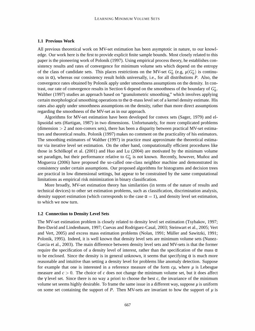
MV-sets summarize regions where the mass ofP is most concentrated. For example, ifP is a mul-tivariate Gaussian distribution andµ is the Lebesgue measure, then the MV-sets are ellipsoids. AnMV-set for a two-component Gaussian mixture is illustrated in Figure 1. Applications of minimumvolume sets include outlier/anomaly detection, determining highest posterior density or multivari-ate confidence regions, tests for multimodality, and clustering. See Polonik (1997); Walther (1997);Scholkopf et al. (2001) and references therein for additional applications.

This paper considers the problem of MV-set estimation using a training sampledrawn fromP, which in most practical settings is the only information one has aboutP. The specifications to

c©2006 Clayton Scott and Robert Nowak.

SCOTT AND NOWAK

Figure 1: Minimum volume set (gray region) of a two-component Gaussian mixture. Also shownare 500 points drawn independently from this distribution.

the estimation process are the significance levelα, the reference measureµ, and a collection ofcandidate setsG .

A major theme of this work is the strong parallel between MV-set estimation and binary classi-fication. In particular, we find that uniform convergence (of true probability to empirical probabilityover the class of setsG ) plays a central role in controlling the performance of MV-set estimators.Thus, we derive distribution free finite sample performance bounds in termsof familiar quantitiessuch as VC dimension. In fact, as we will see, any uniform convergencebound can be directlyconverted to a rule for MV-set estimation.

In Section 2 we introduce a rule for MV-set estimation analogous to empirical risk minimizationin classification, and shows that this rule obeys similar finite sample size performance guarantees.Section 3 extends the results of the previous section to allowG to grow in a controlled way withsample size, leading to MV-set estimators that are strongly universally consistent. Section 4 intro-duces an MV-set estimation rule similar in spirit to structural risk minimization in classification,and develops an oracle-type inequality for this estimator. The oracle inequality guarantees thatthe estimator automatically adapts its complexity to the problem at hand. Section 5 introduces atuning parameter to the proposed rules that allows the user to affect the tradeoff between volumeerror and mass error without sacrificing theoretical properties. Section6 provides a “case study” oftree-structured set estimators to illustrate the power of the oracle inequality for deriving rates of con-vergence. Section 7 includes a set of numerical experiments that explores the proposed theory (andalgorithmic issues) using histogram and decision tree rules in two dimensions. Section 8 includesconcluding remarks and avenues for potential future investigations. Detailed proofs of the mainresults of the paper are relegated to the appendices. Throughout the paper, the theoretical results areillustrated in detail through several examples, including VC classes, histograms, and decision trees.

666

LEARNING M INIMUM VOLUME SETS

1.1 Previous Work

All previous theoretical work on MV-set estimation has been asymptotic in nature, to our knowl-edge. Our work here is the first to provide explicit finite sample bounds. Most closely related to thispaper is the pioneering work of Polonik (1997). Using empirical processtheory, he establishes con-sistency results and rates of convergence for minimum volume sets which depend on the entropyof the class of candidate sets. This places restrictions on the MV-setG∗

α (e.g, µ(G∗α) is continu-

ous inα), whereas our consistency result holds universally, i.e., for all distributionsP. Also, theconvergence rates obtained by Polonik apply under smoothness assumptions on the density. In con-trast, our rate of convergence results in Section 6 depend on the smoothness of the boundary ofG∗

α.Walther (1997) studies an approach based on “granulometric smoothing,”which involves applyingcertain morphological smoothing operations to theα-mass level set of a kernel density estimate. Hisrates also apply under smoothness assumptions on the density, rather than more direct assumptionsregarding the smoothness of the MV-set as in our approach.

Algorithms for MV-set estimation have been developed for convex sets (Sager, 1979) and el-lipsoidal sets (Hartigan, 1987) in two dimensions. Unfortunately, for more complicated problems(dimension> 2 and non-convex sets), there has been a disparity between practical MV-set estima-tors and theoretical results. Polonik (1997) makes no comment on the practicality of his estimators.The smoothing estimators of Walther (1997) in practice must approximate the theoretical estima-tor via iterative level set estimation. On the other hand, computationally efficient procedures likethose in Scholkopf et al. (2001) and Huo and Lu (2004) are motivated by the minimum volumeset paradigm, but their performance relative toG∗

α is not known. Recently, however, Munoz andMoguerza (2006) have proposed the so-called one-class neighbor machine and demonstrated itsconsistency under certain assumptions. Our proposed algorithms for histograms and decision treesare practical in low dimensional settings, but appear to be constrained by the same computationallimitations as empirical risk minimization in binary classification.

More broadly, MV-set estimation theory has similarities (in terms of the nature ofresults andtechnical devices) to other set estimation problems, such as classification, discrimination analysis,density support estimation (which corresponds to the caseα = 1), and density level set estimation,to which we now turn.

1.2 Connection to Density Level Sets

The MV-set estimation problem is closely related to density level set estimation (Tsybakov, 1997;Ben-David and Lindenbaum, 1997; Cuevas and Rodriguez-Casal, 2003; Steinwart et al., 2005; Vertand Vert, 2005) and excess mass estimation problems (Nolan, 1991; Muller and Sawitzki, 1991;Polonik, 1995). Indeed, it is well known that density level sets are minimum volume sets (Nunez-Garcia et al., 2003). The main difference between density level sets and MV-sets is that the formerrequire the specification of a density level of interest, rather than the specification of the massαto be enclosed. Since the density is in general unknown, it seems that specifying α is much morereasonable and intuitive than setting a density level for problems like anomaly detection. Supposefor example that one is interested in a reference measure of the formcµ, whereµ is Lebesguemeasure andc > 0. The choice ofc does not change the minimum volume set, but it does affectthe γ level set. Since there is no way a priori to choose the bestc, the invariance of the minimumvolume set seems highly desirable. To frame the same issue in a different way, supposeµ is uniformon some set containing the support ofP. Then MV-sets are invariant to how the support ofµ is

667

SCOTT AND NOWAK

specified, while density level sets are not. Further advantages of MV-sets over level sets are givenin the concluding section.

Algorithms for density level set estimation can be split into two categories, implicit plug-inmethods and explicit set estimation methods. Plug-in strategies entail full densityestimation andare the more popular practical approach. For example, Baillo et al. (2001) considers plug-in rules fordensity level set estimation problems and establishes upper bounds on the rate of convergence forsuch estimators in certain cases. The problem of estimating a density supportset, the zero level set,is a special minimum volume set (i.e., the minimum volume set that contains the total probabilitymass). Cuevas and Fraiman (1997) study density support estimation and show that a certain (densityestimator) plug-in scheme provides universally consistent support estimation.

While consistency and rate of convergence results for plug-in methods typically make globalsmoothness assumptions on the density, explicit methods make assumptions on thedensity at ornear the level of interest. This fact, together with the intuitive appeal of nothaving to solve aproblem harder than one is interested in, make explicit methods attractive. Steinwart et al. (2005)reduce level set estimation to a cost-sensitive classification problem by sampling from the referencemeasure. The idea of sampling fromµ in the minimum volume context is discussed further in theconcluding section. Vert and Vert (2005) study the one-class support vector machine (SVM) andshow that it produces a consistent density level set estimator, based on the fact that consistent densityestimators produce consistent plug-in level set estimators. Willett and Nowak(2005, 2006) proposea level set estimator based on decision trees, which is applicable to density level set estimation aswell as regression level set estimation, and related dyadic partitioning schemes are developed byKlemela (2004) to estimate the support set of a density.

The connections between MV-sets and density level sets will be important laterin this paper.To make the connection precise the following assumption on the data-generating distribution andreference measure is needed. We emphasize that this assumption is not necessary for the results inSections 2 and 3, where distribution free error bounds and universalconsistency are established.

A1 P has a densityf with respect toµ.

A key result relating density level and MV-sets is the following, stated withoutproof (see, e.g.,Nunez-Garcia et al. (2003)).

Lemma 1 Under assumptionA1 there existsγα such that for any MV-set G∗α,

x : f (x) > γα ⊂ G∗α ⊂ x : f (x) ≥ γα.

Note that every density level set is an MV-set, but not conversely. If,however,µ(x : f (x) = γα) =0, then the three sets in the Lemma coincide.

1.3 Notation

Let (X ,B ) be a measure space withX ⊂ Rd. Let X be a random variable taking values inX with

distribution P. Let S= (X1, . . . ,Xn) be an independent and identically distributed (IID) sampledrawn according toP. Let G denote a subset ofX , and letG be a collection of such subsets. LetPdenote the empirical measure based onS:

P(G) =1n

n

∑i=1

I(Xi ∈ G) .

668

LEARNING M INIMUM VOLUME SETS

Here I(·) is the indicator function. The notationµ will denote a measure1 on X . Denote by fthe density ofP with respect toµ (when it exists),γ > 0 a level of the density, andα ∈ (0,1) auser-specified mass constraint. Define

µ∗α = infG

µ(G) : P(G) ≥ α, (1)

where the inf is over all measurable sets. A minimum volume set,G∗α, is a minimizer of (1) when it

exists.

2. Minimum Volume Sets and Empirical Risk Minimization

We introduce a procedure inspired by the empirical risk minimization (ERM) principle for classifi-cation. In classification, ERM selects a classifier from a fixed set of classifiers by minimizing theempirical error (risk) of a training sample. Vapnik and Chervonenkis established the basic theoret-ical properties of ERM (see Vapnik, 1998; Devroye et al., 1996), andwe find similar properties inthe minimum volume setting.

Let G be a class of sets. Givenα ∈ (0,1), denote

Gα = G∈ G : P(G) ≥ α,

the collection of all sets inG with mass at leastα. Define

µG ,α = infµ(G) : G∈ Gα (2)

andGG ,α = arg minµ(G) : G∈ Gα (3)

when it exists. ThusGG ,α is the best approximation to the minimum volume setG∗α from G .

Empirical versions ofGα andGG ,α are defined as follows. Letφ(G,S,δ) be a function ofG∈ G ,the training sampleS, and a confidence parameterδ ∈ (0,1). Set

Gα = G∈ G : P(G) ≥ α−φ(G,S,δ)

andGG ,α = arg minµ(G) : G∈ Gα. (4)

We refer to the rule in (4) as MV-ERM because of the analogy with empirical risk minimization inclassification. A discussion of the existence and uniqueness of the abovequantities is deferred toSection 2.5.

The quantityφ acts as a kind of “tolerance” by which the empirical mass may deviate from thetargeted valueα. Throughout this paper we assume thatφ satisfies the following.

Definition 2 We sayφ is a (distribution free)complexity penaltyfor G if and only if for all distri-butions P and allδ ∈ (0,1),

Pn

(S: sup

G∈G

(∣∣∣P(G)− P(G)∣∣∣−φ(G,S,δ)

)> 0

)≤ δ.

1. Although we do not emphasize it, the results of Sections 2 and 3 only require µ to be a real-valued function onB .

669

SCOTT AND NOWAK

Thus,φ controls the rate of uniform convergence ofP(G) to P(G) for G∈ G . It is well known thatthe performance of ERM (for binary classification) relative to the performance of the best classifierin the given class is controlled by the uniform convergence of true to empirical probabilities. Asimilar result holds for MV-ERM.

Theorem 3 If φ is a complexity penalty forG , then

Pn((

P(GG ,α) < α−2φ(GG ,α,S,δ))

or(

µ(GG ,α) > µG ,α

))≤ δ.

Proof Consider the sets

ΘP = S: P(GG ,α) < α−2φ(GG ,α,S,δ),Θµ = S: µ(GG ,α) > µ(GG ,α),

ΩP =

S: sup

G∈G

(∣∣∣P(G)− P(G)∣∣∣−φ(G,S,δ)

)> 0

.

Lemma 4 With ΘP,Θµ, andΩP as defined above we have

ΘP∪Θµ ⊂ ΩP.

The proof is given in Appendix A, and follows closely the proof of Lemma 1 inCannon et al.(2002). The theorem statement follows directly from this observation.

Lemma 4 may be understood by analogy with the result from classification that says R ( f )−inf f∈F R ( f ) ≤ 2supf∈F |R ( f )− R ( f )| (see Devroye et al. (1996), Ch. 8). HereR and R are

the true and empirical risks,f is the empirical risk minimizer, andF is a set of classifiers. Justas this result relates uniform convergence to empirical risk minimization in classification, so doesLemma 4 relate uniform convergence to the performance of MV-ERM.

The theorem above allows direct translation of uniform convergence results into performanceguarantees on MV-ERM. Fortunately, many penalties (uniform convergence results) are known. Inthe next two subsections we take a closer look at penalties for VC classes and countable classes,and a Rademacher penalty.

2.1 Example: VC Classes

Let G be a class of sets with VC dimensionV, and define

φ(G,S,δ) =

√32

V logn+ log(8/δ)

n. (5)

By a version of the VC inequality (Devroye et al., 1996), we know thatφ is a complexity penaltyfor G , and therefore Theorem 3 applies.

To view this result in perhaps a more recognizable way, letε > 0 and chooseδ such thatφ(G,S,δ) = ε for all G ∈ G and all S. By inverting the relationship betweenδ and ε, we havethe following.

670

LEARNING M INIMUM VOLUME SETS

Corollary 5 With the notation defined above,

Pn((

P(GG ,α) < α−2ε)

or(

µ(GG ,α) > µG ,α

))≤ 8nVe−nε2/128.

Thus, for any fixedε > 0, the probability of being within 2ε of the target massα and being less thanthe target volumeµG ,α approaches one exponentially fast as the sample size increases. This resultmay also be used to calculate a distribution free upper bound on the sample sizeneeded to be withina given toleranceε of α and with a given confidence 1−δ. In particular, the sample size will growno faster than a polynomial in 1/ε and 1/δ, paralleling results for classification.

2.2 Example: Countable Classes

SupposeG is a countable class of sets. Assume that to everyG∈ G a numberJGK is assigned suchthat

∑G∈G

2−JGK ≤ 1. (6)

In light of the Kraft inequality for prefix2 codes (Cover and Thomas, 1991),JGK may be defined asthe codelength of a codeword forG in a prefix code forG . Let δ > 0 and define

φ(G,S,δ) =

√JGK log2+ log(2/δ)

2n. (7)

By Chernoff’s bound together with the union bound,φ is a penalty forG . Therefore Theorem 3applies and we have a result analogous to the Occam’s Razor bound for classification (see Langford,2005).

As a special case, supposeG is finite and takeJGK = log2 |G |. Settingε = φ(G,S,δ) and invert-ing the relationship betweenδ andε, we have the following.

Corollary 6 For the MV-ERM estimateGG ,α from a finite classG

Pn((

P(GG ,α) < α−2ε)

or(

µ(GG ,α) > µG ,α

))≤ 2|G |e−nε2/2.

As with VC classes, these inequalities may be used for sample size calculations.

2.3 The Rademacher Penalty for Sets

The Rademacher penalty was originally studied in the context of classificationby Koltchinskii(2001) and Bartlett et al. (2002). For a succinct exposition of its basic properties, see Bousquetet al. (2004). An analogous penalty exists for sets. Letσ1, . . . ,σn be Rademacher random variables,i.e., independent random variables taking on the values 1 and -1 with equalprobability. DenoteP(σi)(G) = 1

n ∑ni=1 σiI(Xi ∈ G). We define the Rademacher average

ρ(G ) = E

[supG∈G

P(σi)(G)

]

2. A prefix code is a collection of codewords (strings of 0s and 1s) suchthat no codeword is a prefix of another.

671

SCOTT AND NOWAK

and the conditional Rademacher average

ρ(G ,S) = E(σi)

[supG∈G

P(σi)(G)

],

where the second expectation is with respect the Rademacher random variables only, and condi-tioned on the sampleS.

Proposition 7 With probability at least1−δ over the draw of S,

P(G)− P(G) ≤ 2ρ(G )+

√log(1/δ)

2n

for all G ∈ G . With probability at least1−δ over the draw of S,

P(G)− P(G) ≤ 2ρ(G ,S)+

√2log(2/δ)

n

for all G ∈ G .

The proof of this result follows exactly the same lines as the proof of Theorem 5 in Bousquet et al.(2004), and is omitted.

AssumeG satisfies the property thatG ∈ G ⇒ G ∈ G , whereG denotes the compliment ofG. Then P(G)−P(G) = P(G)− P(G), and so the upper bounds of Proposition 7 also apply to|P(G)− P(G)|. Thus we are able to define the conditional Rademacher penalty

φ(G,S,δ) = 2ρ(G ,S)+

√2log(2/δ)

n.

By the above Proposition, this is a complexity penalty according to Definition 2. The conditionalRademacher penalty is studied further in Section 7 and in Appendix E, whereit is shown thatρ(G ,S)can be computed efficiently for sets based on a fixed partition ofX (such as histograms and trees).

2.4 Comparison to Generalized Quantile Processes

Polonik (1997) studies theempirical quantile function

Vα = infµ(G) : P(G) ≥ α,

and the MV-set estimate that achieves the minimum (when it exists). The only difference comparedwith MV-ERM is the absence of the termφ(G,S,δ) in the constraint. Thus, MV-ERM will tend toproduce estimates with smaller volume and smaller mass. While Polonik proves only asymptoticproperties of his estimator, we have demonstrated finite sample bounds for MV-ERM. Moreover,in Section 5, we show that the results of this section extend to a generalization of MV-ERM whereφ is replaced byνφ, whereν is any number−1≤ ν ≤ 1. Thus finite sample bounds also exist forPolonik’s estimator (ν = 0).

672

LEARNING M INIMUM VOLUME SETS

2.5 Existence and Uniqueness

In this section we discuss the existence and uniqueness of the setsGG ,α andGG ,α. Regarding theformer, it is really not necessary that a minimizer exist. All of our results arestated in terms ofµG ,α,which certainly exists. When a minimizer exists, its uniqueness is not an issue for the same reason.Our results above involve onlyµG ,α, which is the same regardless of which minimizer is chosen.Yet one may wonder whether convergence of the volume and mass to their optimal values impliesconvergence to the MV-set (when it is unique) in any sense. A result in this direction is presented inTheorem 10 below.

For the MV-ERM estimateGG ,α, uniqueness is again not an issue because all results hold evenif the minimizer is chosen arbitrarily. As for existence, we must be more careful. We cannot makethe same argument as forGG ,α because we are ultimately interested in a concrete set estimate, not

just its volume and mass. Clearly, ifG is finite, GG ,α exists. For more general sets, existence mustbe examined on a case-by-case basis. For example, ifX ⊂ R

d, µ is the Lebesgue measure, andG isthe VC class of spherical or ellipsoidal sets, thenGG ,α can be seen to exist.

In the event thatGG ,α does not exist, it suffices to letGG ,α be a set whose volume comes within

ε of the infimum, whereε is arbitrarily small. Then our results still hold withµ(GG ,α) replaced by

µ(GG ,α)−ε. The consistency and rate of convergence results below are unchanged, as we may takeε → 0 arbitrarily fast as a function ofn.

3. Consistency

A minimum volume set estimator is consistent if its volume and mass tend to the optimal valuesµ∗αandα asn→ ∞. Formally, define the error quantity

E (G) := (µ(G)−µ∗α)+ +(α−P(G))+ ,

where(x)+ = max(x,0). We are interested in MV-set estimators such thatE (GG ,α) tends to zero asn→ ∞.

Definition 8 A learning ruleGG ,α is strongly consistentif

limn→∞E (GG ,α) = 0 with probability 1.

If GG ,α is strongly consistent for every possible distribution of X, thenGG ,α is stronglyuniversallyconsistent.

In this section we show that if the approximating power ofG increases in a certain way as a functionof n, then MV-ERM leads to a universally consistent learning rule.

To see how consistency might result from MV-ERM, it helps to rewrite Theorem 3 as follows.Let G be fixed and letφ(G,S,δ) be a penalty forG . Then with probability at least 1−δ, both

µ(GG ,α)−µ∗α ≤ µ(GG ,α)−µ∗α (8)

andα−P(GG ,α) ≤ 2φ(GG ,α,S,δ) (9)

673

SCOTT AND NOWAK

hold. We refer to the left-hand side of (8) as theexcess volumeof the classG and the left-hand sideof (9) as themissing massof GG ,α. The upper bounds on the right-hand sides are an approximationerror and a stochastic error, respectively.

The idea is to letG grow with n so that both errors tend to zero asn → ∞. If G does notchange withn, universal consistency is impossible. Either the approximation error will benonzerofor most distributions (whenG is too small) or the bound on the stochastic error will be too large(otherwise). For example, if a class has universal approximation capabilities, its VC dimension isnecessarily infinite (Devroye et al., 1996, Ch. 18).

To have both stochastic and approximation errors tend to zero, we apply MV-ERM to a classG k from a sequence of classesG 1,G 2, . . ., wherek = k(n) grows with the sample size. Given sucha sequence, define

GG k,α = arg minµ(G) : G∈ G kα, (10)

whereG k

α = G∈ G k : P(G) ≥ α−φk(G,S,δ)andφk is a penalty forG k.

Theorem 9 Choose k= k(n) andδ = δ(n) such that

1. k(n) → ∞ as n→ ∞

2. ∑∞n=1 δ(n) < ∞

Assume the sequence of setsG k and penaltiesφk satisfy

limk→∞

infG∈G k

α

µ(G) = µ∗α (11)

andlimn→∞

supG∈G k

φk(G,S,δ(n)) = 0. (12)

ThenGG k,α is strongly universally consistent.

The proof is given in Appendix B. We now give some examples that satisfy these conditions.

3.1 Example: Hierarchy of VC Classes

AssumeG 1,G 2, . . . , is a family of VC classes with VC dimensionsV1 <V2 < .. . . ForG∈ G k define

φk(G,S,δ) =

√32

Vk logn+ log(8/δ)

n. (13)

By taking δ(n) ≍ n−β for someβ > 1 andk such thatVk = o(n/ logn) the assumption in (12) issatisfied. Examples of families of VC classes satisfying (11) include generalized linear discriminantrules with appropriately chosen basis functions and neural networks (Lugosi and Zeger, 1995).

674

LEARNING M INIMUM VOLUME SETS

3.2 Example: Histograms

AssumeX = [0,1]d, and letG k be the class of all sets formed by taking unions of cells in a regularpartition ofX into hypercubes of sidelength 1/k. EachG k has 2k

dmembers and we may therefore

apply the penalty for finite sets discussed in Section 2.2. To satisfy the Kraftinequality (6) it sufficesto takeJGK = kd. The penalty forG∈ G k is then

φk(G,S,δ) =

√kd log2+ log(2/δ)

2n. (14)

By taking δ(n) ≍ n−β for someβ > 1 andk such thatkd = o(n) the assumption in (12) is satis-fied. The assumption in (11) is satisfied by the well-known universal approximation capabilities ofhistograms. Thus the conditions for consistency of histograms for minimum volume set estimationare exactly parallel to the conditions for consistency of histogram rules for classification (Devroyeet al., 1996, Ch. 9). Dyadic decision trees, discussed below in Section 6,are another countablefamily for which consistency results are possible.

3.3 The Symmetric Difference Performance Metric

An alternative measure of performance for an MV-set estimator is theµ-measure of the symmetricdifference,µ(GG ,α∆G∗

α), whereA∆B = (A\B)∪ (B\A). Although this performance metric has beencommonly adopted in the study of density level sets, it is less desirable for ourpurposes. First, unlikewith density level sets, there may not be a unique MV-set (imagine the case where the density ofPhas a plateau). Second, as pointed out by Steinwart et al. (2005), there is no known way to estimatethe accuracy of this measure using only samples fromP. Nonetheless, the symmetric differencemetric coincides asymptotically with our error metricE in the sense of the following result. Thetheorem uses the notationγα to denote the density level corresponding to the MV-set, as discussedin Section 1.2.

Theorem 10 Assume µ is a probability measure and P has a density f with respect to µ. LetGn denote a sequence of sets. If G∗

α is a minimum volume set and µ(Gn∆G∗α) → 0 with n, then

E (Gn) → 0. Conversely, assume µ(x : f (x) = γα) = 0. If E (Gn) → 0, then µ(Gn∆G∗α) → 0.

The proof is given in Appendix C. The assumption of the second part of the theorem ensuresthat G∗

α is unique, otherwise the converse statement need not be true. The proofof the conversereveals yet another connection between MV-set estimation and classification. In particular, weshow thatE (Gn) bounds the excess classification risk for a certain classification problem. Theconverse statement then follows from a result of Steinwart et al. (2005)who show that this excessclassification risk and theµ-measure of the symmetric difference tend to zero simultaneously.

4. Structural Risk Minimization and an Oracle Inequality

In the previous section on consistency the rate of convergence of the twoerrors to zero is determinedby the choice ofk= k(n), which must be chosen a priori. Hence it is possible that the excess volumedecays much more quickly than the missing mass, or vice versa. In this section we introduce a newrule called MV-SRM, inspired by the principle of structural risk minimization (SRM) from thetheory of classification (Vapnik, 1982; Lugosi and Zeger, 1996), that automatically balances thetwo errors.

675

SCOTT AND NOWAK

The results of this and subsequent sections are no longer distribution free. In particular, weassume

A1 P has a densityf with respect toµ.

A2 for all α′ ∈ (0,1), G∗α′ exists andP(G∗

α′) = α′.

Note thatA2 holds if f has no plateaus, i.e.,µ(x : f (x) = γ) = 0 for all γ > 0. This is a commonlymade assumption in the study of density level sets. However,A2 is somewhat more general. It stillholds, for example, ifµ is absolutely continuous with respect to Lebesgue measure, even iff hasplateaus.

Recall from Section 1.2 that under assumptionA1, there existsγα > 0 such for any MV-setG∗α,

x : f (x) > γα ⊂ G∗α ⊂ x : f (x) ≥ γα.

Let G be a class of sets. Intuitively, viewG as a collection of sets of varying capacities, suchas a union of VC classes or a union of finite classes (examples are given below). Letφ(G,S,δ) be apenalty forG . The MV-SRM principle selects the set

GG ,α = arg minG∈G

µ(G)+2φ(G,S,δ) : P(G) ≥ α−φ(G,S,δ)

. (15)

Note that MV-SRM is different from MV-ERM because it minimizes a complexity penalized vol-ume instead of simply the volume. We have the following oracle inequality for MV-SRM. RecallE (G) := (µ(G)−µ∗α)+ +(α−P(G))+.

Theorem 11 Let GG ,α be the MV-set estimator in (15) and assumeA1 andA2 hold. With proba-bility at least1−δ over the training sample S,

E (GG ,α) ≤(

1+1γα

)inf

G∈Gα

µ(G)−µ∗α +2φ(G,S,δ)

. (16)

Although the value of 1/γα is in practice unknown, it can be bounded by

1γα

≤ µ(X )−µ∗α1−α

≤ µ(X )

1−α.

This follows from the bound 1−α ≤ γα · (µ(X )−µ∗α) on the mass outside the minimum volume set.If µ is a probability measure, then 1/γα ≤ 1/(1−α).

The oracle inequality says that MV-SRM performs about as well as the setchosen by an oracleto optimize the tradeoff between excess volume and missing mass.

4.1 Example: Union of VC Classes

ConsiderG = ∪Kk=1G

k, whereG k has VC dimensionVk, V1 < V2 < · · · , andK is possibly infinite.A penalty forG can be obtained by defining, forG∈ G k,

φ(G,S,δ) = φk(G,S,δ2−k),

whereφk is the penalty from Equation (13). Thenφ is a penalty forG becauseφk is a penalty forG k, and by applying the union bound and the fact∑k≥12−k ≤ 1. In this case, MV-SRM adaptively

676

LEARNING M INIMUM VOLUME SETS

selects an MV-set estimate from a VC class that balances approximation and stochastic errors. Notethat instead of settingδk = δ2−k one could also chooseδk ∝ k−β,β > 1.

To be more concrete, supposeG k is the collection of sets whose boundaries are defined by poly-nomials of degreek. It may happen that for certain distributions, the MV-set is well-approximatedby a quadratic region (such as an ellipse), while for other distributions a higher degree polynomialis required. If the appropriate polynomial degree for the MV-set is not known in advance, as wouldbe the case in practice, then MV-SRM adaptively chooses an estimator of a certain degree that doesabout as well as if the best degree was known in advance.

4.2 Example: Union of Histograms

Let G = ∪Kk=1G

k, whereG k is as in Section 3.2. As with VC classes, we obtain a penalty forG bydefining, forG∈ G k,

φ(G,S,δ) = φk(G,S,δ2−k),

whereφk is the penalty from Equation (14). Then MV-SRM adaptively chooses a partition resolutionk that approximates the MV-set about as well as possible without overfitting the training data. Thisexample is studied experimentally in Section 7.

5. Damping the Penalty

In Theorem 3, the reader may have noticed that MV-ERM does not equitably balance the excessvolume (µ(GG ,α) relative to its optimal value) with the missing mass (P(GG ,α) relative toα). Indeed,

with high probability,µ(GG ,α) is less than µ(GG ,α), while P(GG ,α) is only guaranteed to be within

2φ(GG ,α) of α. The net effect is that MV-ERM (and MV-SRM) underestimates the MV-set. Ourexperiments in Section 7 demonstrate this to be the case.

In this section we introduce variants of MV-ERM and MV-SRM that allow the total error tobe shared between the volume and mass, instead of all of the error residingin the mass term. Ourapproach is to introduce a damping factor−1≤ ν ≤ 1 that scales the penalty. We will see that theresulting MV-set estimators obey performance guarantees like those we have already seen, but withthe total error redistributed between the volume and mass. The reason for not introducing this moregeneral framework initially is that the results are slightly less general, more involved to state, and tosome extent follow as corollaries to the original (ν = 1) framework.

The extensions of this section encompass the generalized quantile estimate of Polonik (1997),which corresponds toν = 0. Thus we have finite sample size guarantees for that estimator to matchPolonik’s asymptotic analysis. The caseν = −1 is also of interest. If it is crucial that the estimatesatisfies the mass constraintP(GG ,α) ≥ α (note that this involves thetrue probability measureP),settingν = −1 ensures this to be the case with probability at least 1−δ.

First we consider damping the penalty in MV-ERM. Assume that the penalty is independent ofG ∈ G and of the sampleS, although it can depend onn andδ. That is,φ(G,S,δ) = φ(n,δ). Forexample,φ may be the penalty in (5) for VC classes or (7) for finite classes. Letν ≤ 1 and define

GνG ,α = arg min

G∈G

µ(G) : P(G) ≥ α−νφ(n,δ)

.

677

SCOTT AND NOWAK

Sinceφ is independent ofG∈ G , GνG ,α coincides with the MV-ERM estimate (as originally formu-

lated)GG ,α′ but at the adjusted mass constraintα′ = α +(1−ν)φ(n,δ). Therefore, we may applyTheorem 3 to obtain the following.

Corollary 12 Let α′ = α+(1−ν)φ(n,δ). Then

Pn((

P(GνG ,α) < α− (1+ν)φ(n,δ)

)or(

µ(GG ,α) > µG ,α′)))

≤ δ.

Relative to the original formulation of MV-ERM, the bound on the missing mass is decreasedby a factor(1+ν). On the other hand, the volume is now bounded byµG ,α′ = µG ,α +(µG ,α′ −µG ,α).Thus the bound on the excess volume is increased from 0 toµG ,α′ −µG ,α. This may be interpreted

as a stochastic component of the excess volume. Relative to the MV-set,µ(GG ,α) has only an

approximation error, whereasµ(GνG ,α) has both approximation and stochastic errors. The advantage

is that now the stochastic error of the mass is decreased.A similar construction applies to MV-SRM. Now assumeG =∪K

k=1Gk. Given a scale parameter

ν, defineGνG ,α = arg min

G∈G

µ(G)+(1+ν)φ(G,S,δ) : P(G) ≥ α−νφ(G,S,δ)

.

As above, assumeφ is independent of the sample and constant on eachG k. Denoteεk(n,δ) =φ(G,S,δ) for G ∈ G k. Observe that computingGν

G ,α is equivalent to computing the MV-ERM

estimate on eachG k at the levelα(k,ν) = α +(1− ν)εk(n,δ), and then minimizing the penalizedvolume over these MV-ERM estimates.

Like the original MV-SRM, this modified procedure also obeys an oracle inequality. Recall thenotationG k

α(k,ν) = G∈ G k : P(G) ≥ α(k,ν) = G∈ G k : P(G) ≥ α+(1−ν)εk(n,δ).

Theorem 13 Let −1 ≤ ν ≤ 1. Setα(k,ν) = α +(1− ν)εk(n,δ). AssumeA1 and A2 hold. Withprobability at least1−δ,

E (GνG ,α) ≤

(1+

1γα

)min

1≤k≤K

[inf

G∈G kα(k,ν)

µ(G)−µ∗α(k,ν)

+Ckεk(n,δ)

], (17)

where Ck =((1+ν)+ 1

γα(k,ν)(1−ν)

).

Hereγα(k,ν) is the density level corresponding to the MV-set with massα(k,ν). It may be boundedabove in terms of known quantities, as discussed in the previous section. The proof of the theoremis very similar to the proof of the earlier oracle inequality and is omitted, although itmay be foundin Scott and Nowak (2005a). Notice that in the caseν = 1 we recover Theorem 11 (under the statedassumptions onG andφ). Also note thatG k

α(k,ν) will be empty if α(k,ν) > 1, in which case thosekshould be excluded from the min.

To understand the result, assume that the rate at whichG kα approximatesG∗

α is independent ofα.In other words, the rate at which infG∈G k

αµ(G)−µ∗α tends to zero ask increases is the same for allα.

Then in the theorem we may replace the expression infG∈G kα(k,ν)

µ(G)−µ∗α(k,ν) with infG∈G kαµ(G)−µ∗α.

Thus, theν-damped MV-SRM error decays at the same rate is the original MV-SRM, and adaptivelyselects the appropriate model classG k from which to draw the estimate. Furthermore, damping the

678

LEARNING M INIMUM VOLUME SETS

penalty byν has the effect of decreasing the stochastic mass error and adding a stochastic errorto the volume. This follows from the above discussion of MV-ERM and the observation that theMV-SRM coincides with an MV-SRM estimate overG k for somek. The improved balancing ofvolume and mass error is confirmed by our experiments in Section 7.

6. Rates of Convergence for Tree-Structured Set Estimators

In this section we illustrate the application of MV-SRM, when combined with an appropriate anal-ysis of the approximation error, to the study of rates of convergence. Topreview the main result ofthis section (Theorem 16), we will consider the class of distributions such that the decision bound-ary has Lipschitz smoothness (loosely speaking) andd′ of thed features are relevant. The best rateof convergence for this class isn−1/d′

. We will show that MV-SRM can achieve this rate (within alog factor) without knowingd′ or which features are relevant. This demonstrates the strength of theoracle inequality, from which the result is derived.

To obtain these rates we apply MV-SRM to sets based on a special family of decision treescalled dyadic decision trees (DDTs) (Scott and Nowak, 2006). Beforeintroducing DDTs, however,we first introduce the class of distributionsD with which our study is concerned. Throughout thissection we assumeX = [0,1]d andµ is the Lebesgue (equivalently, uniform) measure.

Somewhat related to the approach considered here is the work of Klemela (2004) who consid-ers the problem of estimating the support of a uniform density. The estimatorsproposed thereinare based on dyadic partitioning schemes similar in spirit to the DDTs studied here. However,it is important to point out that in the support set estimation problem studied by Klemela (2004)the boundary of the set corresponds to discontinuity of the density, and therefore more standardcomplexity-regularization and tree pruning methods commonly employed in regression settings suf-fice to achieve near minimax rates. In contrast, DDT methods are capable of attaining near minimaxrates for all density level sets whose boundaries belong to certain Holder smoothness classes, regard-less of whether or not there is a discontinuity at the given level. Significantlydifferent risk boundingand pruning techniques are required for this additional capability (Scott and Nowak, 2006).

6.1 The Box-Counting Class

Before introducingD we need some additional notation. Letmdenote a positive integer, and definePm to be the collection ofmd cells formed by the regular partition of[0,1]d into hypercubes ofsidelength 1/m. Letc1,c2 > 0 be positive real numbers. LetG∗

α be a minimum volume set, assumedto exist, and let∂G∗

α be the topological boundary ofG∗α. Finally, letNm(∂G∗

α) denote the number ofcells inPm that intersect∂G∗

α.We define thebox-countingclass to be the setD BOX =D BOX(c1,c2) of all distributions satisfying

A1’ : X has a densityf with respect toµ and f is essentially bounded byc1.

A3 : ∃G∗α such thatNm(∂G∗

α) ≤ c2md−1 for all m.

Note that sinceµ is the Lebesgue measure, assumptionA2 from above follows fromA1, so we donot need to assume it explicitly here. AssumptionA1’ is a slight strengthening ofA1 and impliesP(A) ≤ c1µ(A) for all measurable setsA. AssumptionA3 essentially requires the boundary of theminimum volume setG∗

α to have Lipschitz smoothness, and thus one would expect the optimal rate

679

SCOTT AND NOWAK

Figure 2: A dyadic decision tree (right) with the associated recursive dyadic partition (left) ind = 2dimensions. Each internal node of the tree is labeled with an integer from 1 tod indicatingthe coordinate being split at that node. The leaf nodes are decorated withclass labels.

of convergence to ben−1/d (the typical rate for set estimation problems characterized by Lipschitzsmoothness). See Scott and Nowak (2006) for further discussion of the box-counting assumption.

6.2 Dyadic Decision Trees

Let T denote a tree structured classifierT : [0,1]d → 0,1. Each suchT gives rise to a setGT =x∈ [0,1]d : T(x) = 1. In this subsection we introduce a certain class of trees, and later considerMV-SRM over the induced class of sets.

Scott and Nowak (2006) demonstrate thatdyadic decision trees(DDTs) offer a computationallyfeasible classifier that also achieves optimal rates of convergence (forstandard classification) undera wide range of conditions. DDTs are especially well suited for rate of convergence studies. Indeed,bounding the approximation error is handled by the restriction to dyadic splits,which allows usto take advantage of recent insights from multiresolution analysis and nonlinear approximations(DeVore, 1998; Cohen et al., 2001; Donoho, 1999). An analysis similarto that of Scott and Nowak(2006) applies to MV-SRM for DDTs, leading to similar results: optimal rates ofconvergence for acomputationally efficient learning algorithm.

A dyadic decision tree is a decision tree that divides the input space by means of axis-orthogonaldyadic splits. More precisely, a DDTT is a binary tree (with a distinguished root node) specifiedby assigning (1) an integerc(v) ∈ 1, . . . ,d to each internal nodev of T (corresponding to thecoordinate that gets split at that node); (2) a binary label 0 or 1 to each leaf node ofT. The nodesof DDTs correspond to hyperrectangles (cells) in[0,1]d. Given a hyperrectangleA = ∏d

c=1[ac,bc],let Ac,1 andAc,2 denote the hyperrectangles formed by splittingA at its midpoint along coordinatec. Specifically, defineAc,1 = x∈ A | xc ≤ (ac +bc)/2 andAc,2 = A\Ac,1.

Each node ofT is associated with a cell according to the following rules: (1) The root nodeisassociated with[0,1]d; (2) If v is an internal node associated with the cellA, then the children ofv areassociated withAc(v),1 andAc(v),2. See Figure 2. Note that everyT corresponds to a setGT ∈ [0,1]d

(the regions labeled 1), and we think of DDTs as both classifiers and sets interchangeably.

680

LEARNING M INIMUM VOLUME SETS

Let L = L(n) be a natural number and defineT L to be the collection of all DDTs such that (1) noleaf cell has a sidelength smaller than 2−L, and (2) any two leaf nodes that are siblings have differentlabels. Condition (1) says that when traversing a path from the root to a leaf no coordinate is splitmore thanL times. Condition (2) means that it is impossible to “prune” at any internal node andstill have the same set/classifier. Also defineA L to be the collection of all cellsA that correspondto nodes of DDTs inT L. Defineπ(T) to be the collection of “leaf” cells ofT. For a cellA∈ A L,let j(A) denote the depth ofA when viewed as a node in some DDT. Observe that whenµ is theLebesgue measure,µ(A) = 2− j(A).

6.3 MV-SRM with Dyadic Decision Trees

We study MV-SRM over the familyG L = GT : T ∈ T L, whereL is set by the user. To simplifythe notation, at times we will suppress the dependence ofφ on the training sampleSand confidenceparameterδ. Thus our MV set estimator has the form

Gα = arg minG∈G L

µ(G)+2φ(G) | P(G)+φ(G) ≥ α

. (18)

It remains to specify the penaltyφ. There are a number of ways to produceφ satisfying

Pn

(S: sup

G∈G L

(∣∣∣P(G)− P(G)∣∣∣−φ(G,S,δ)

)> 0

)≤ δ.

SinceG L is countable (in fact, finite), one approach is to devise a prefix code forG L and apply thepenalty in Section 2.2. Instead, we employ a different penalty which has the advantage that it leadsto minimax optimal rates of convergence. Introduce the notationJAK = (3+ log2d) j(A), which maybe thought of as the codelength ofA in a prefix code forA L, and define theminimaxpenalty

φ(GT) := ∑A∈π(T)

√

8max

(P(A),

JAK log2+ log(2/δ)

n

)JAK log2+ log(2/δ)

n. (19)

For eachA∈ π(T), setℓ(A) = 1 if A⊂ GT and 0 otherwise. The bound originates from writing

P(GT)− P(GT) = ∑A∈π(T):ℓ(A)=1

P(A)− P(A)

and

P(GT)−P(GT) = P(GT)− P(GT)

= ∑A∈π(T):ℓ(A)=0

P(A)− P(A)

from which it follows that

|P(GT)− P(GT)| ≤ ∑A∈π(T)

P(A)− P(A). (20)

The eventX ∈ A is a Bernoulli trial with probability of successP(A), and so bounding the righthand side of (20) simply involves applying a concentration inequality for binomials to eachA∈ A L.

681

SCOTT AND NOWAK

There are many ways to do this (additive Chernoff, relative Chernoff,exact tail inversion, etc.),but the one we have chosen is particularly convenient for rate of convergence analysis. For furtherdiscussion, see Scott and Nowak (2006). Proof of the following resultis nearly identical to a similarresult in Scott and Nowak (2006), and is omitted.

Proposition 14 Let φ be as in (19) and letδ ∈ (0,1). With probability at least1−δ over the drawof S,

|P(G)− P(G)| ≤ φ(G)

for all G ∈ G L. Thusφ is a complexity penalty forG L.

The MV-SRM procedure overG L with the above penalty leads to an optimal rate of convergencefor the box-counting class.

Theorem 15 Choose L= L(n) andδ = δ(n) such that

1. 2L(n) < (n/ logn)1/d

2. δ(n) = O(√

logn/n) and log(1/δ(n)) = O(logn)

DefineGα as in (18) withφ as in (19). For d≥ 2 we have

supDBOX

EnE (Gα) 4

(logn

n

) 1d

. (21)

We omit the proof, since this theorem is a special case of Theorem 16 below. Note that the conditionon δ is satisfied ifδ(n) ≍ n−β for someβ > 1/2.

6.4 Adapting to Relevant Features

The previous result could have been obtained without using MV-SRM. Instead, we could haveapplied MV-ERM to a fixed hierarchyG L(1),G L(2), . . . whereL(n) ≍ (n/ logn)1/d. The strength ofMV-SRM and the associated oracle inequality is in its ability to adapt to favorableconditions on thedata generating distribution which may not be known in advance. Here we illustrate this idea whenthe number of relevant features is not known in advance.

We define therelevant data dimensionto be the numberd′ ≤ d of relevant features. A featureXi , i = 1, . . . ,d, is said to be relevant providedf (X) is not constant whenXi is varied from 0 to 1.For example, ifd = 2 andd′ = 1, then∂G∗

α is a horizontal or vertical line segment (or union of suchline segments). Ifd = 3 andd′ = 1, then∂G∗

α is a plane (or union of planes) orthogonal to one ofthe axes. Ifd = 3 and the third coordinate is irrelevant (d′ = 2), then∂G∗

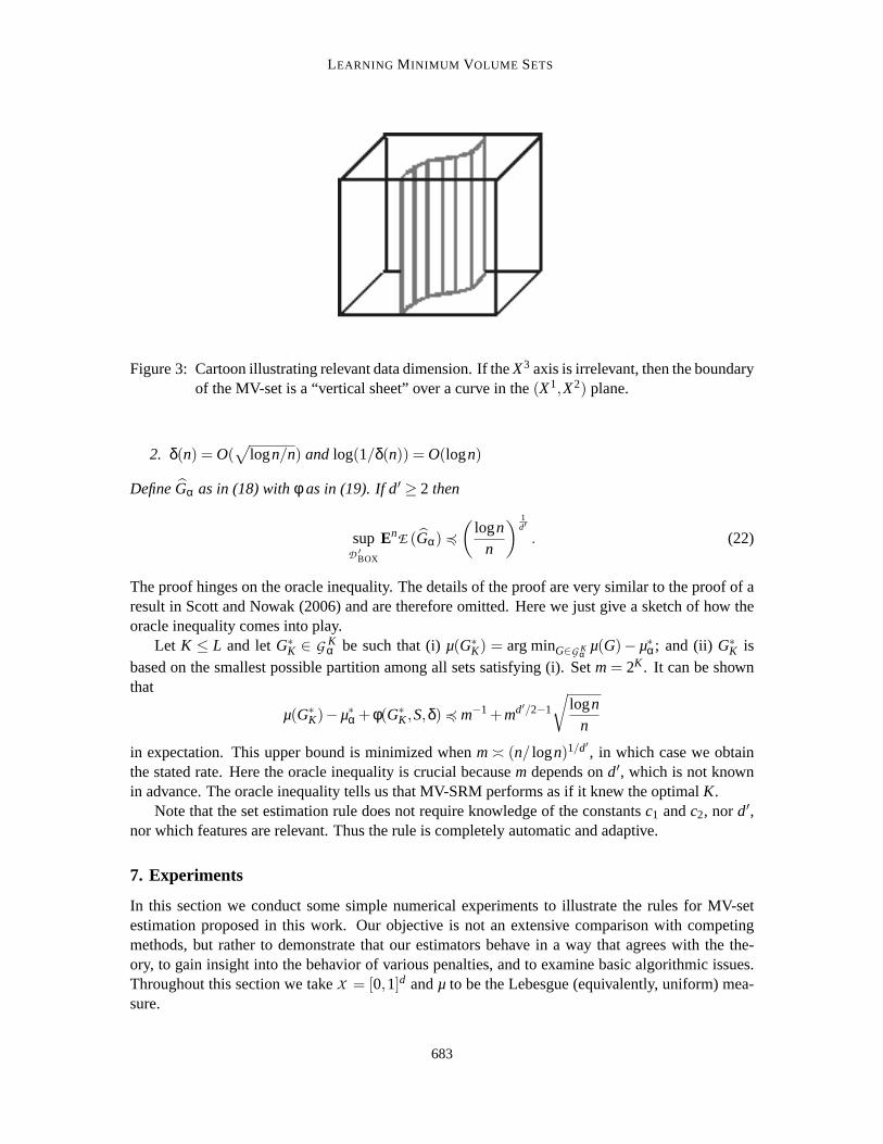
α is a “vertical sheet” overa curve in the(X1,X2) plane (see Figure 3).

Let D ′BOX = D ′

BOX(c1,c2,d′) be the set of all product measuresPn such thatA1’ andA3 holdfor the underlying distributionP, andX has relevant data dimensiond′ ≥ 2. An argument of Scottand Nowak (2006) implies that the expected minimax rate ford′ relevant features isn−1/d′

. By thefollowing result, MV-SRM can achieve this rate to within a log factor.

Theorem 16 Choose L= L(n) andδ = δ(n) such that

1. 2L(n) < n/ logn

682

LEARNING M INIMUM VOLUME SETS

Figure 3: Cartoon illustrating relevant data dimension. If theX3 axis is irrelevant, then the boundaryof the MV-set is a “vertical sheet” over a curve in the(X1,X2) plane.

2. δ(n) = O(√

logn/n) and log(1/δ(n)) = O(logn)

DefineGα as in (18) withφ as in (19). If d′ ≥ 2 then

supD ′

BOX

EnE (Gα) 4

(logn

n

) 1d′

. (22)

The proof hinges on the oracle inequality. The details of the proof are very similar to the proof of aresult in Scott and Nowak (2006) and are therefore omitted. Here we justgive a sketch of how theoracle inequality comes into play.

Let K ≤ L and letG∗K ∈ G K

α be such that (i)µ(G∗K) = arg minG∈G K

αµ(G)−µ∗α; and (ii) G∗

K isbased on the smallest possible partition among all sets satisfying (i). Setm= 2K . It can be shownthat

µ(G∗K)−µ∗α +φ(G∗

K ,S,δ) 4 m−1 +md′/2−1

√logn

n

in expectation. This upper bound is minimized whenm≍ (n/ logn)1/d′, in which case we obtain

the stated rate. Here the oracle inequality is crucial becausem depends ond′, which is not knownin advance. The oracle inequality tells us that MV-SRM performs as if it knewthe optimalK.

Note that the set estimation rule does not require knowledge of the constantsc1 andc2, nord′,nor which features are relevant. Thus the rule is completely automatic and adaptive.

7. Experiments

In this section we conduct some simple numerical experiments to illustrate the rulesfor MV-setestimation proposed in this work. Our objective is not an extensive comparison with competingmethods, but rather to demonstrate that our estimators behave in a way that agrees with the the-ory, to gain insight into the behavior of various penalties, and to examine basic algorithmic issues.Throughout this section we takeX = [0,1]d andµ to be the Lebesgue (equivalently, uniform) mea-sure.

683

SCOTT AND NOWAK

7.1 Histograms

We devised a simple numerical experiment to illustrate MV-SRM in the case of histograms (seeSections 3.2 and 4.2). In this case, MV-SRM can be implemented exactly with a simple procedure.First, compute the MV-ERM estimate for eachG k, k = 1, . . . ,K, where 1/k is the bin-width. To dothis, for eachk, sort the cells of the partition according to the number of samples in the cell. Then,begin incorporating cells into the estimate one cell at a time, starting with the most populated, untilthe empirical mass constraint is satisfied. Finally, once all MV-ERM estimates have been computed,choose the one that minimizes the penalized volume.

We consider two penalties. Both penalties are defined viaφ(G,S,δ) = φk(G,S,δ2−k) for G∈ G k,whereφk is a penalty forG k. The first is based on the simple Occam-style bound of Section 3.2.ForG∈ G k, set

φOcck (G,S,δ) =

√kd log2+ log(2/δ)

2n.

The second is the (conditional) Rademacher penalty. ForG∈ G k, set

φRadk (G,S,δ) =

2n

E(σi)

[sup

G′∈G k

n

∑i=1

σiI(Xi ∈ G′)

]+

√2log(2/δ)

n.

Hereσ1, . . . ,σn are Rademacher random variables, i.e., independent random variablestaking on thevalues 1 and -1 with equal probability. Fortunately, the conditional expectation with respect to thesevariables can be evaluated exactly in the case of partition-based rules such as the histogram. SeeAppendix E for details.

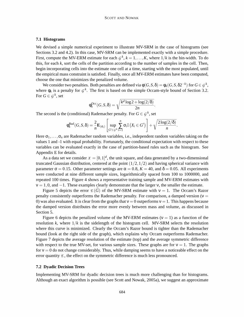
As a data set we considerX = [0,1]d, the unit square, and data generated by a two-dimensionaltruncated Gaussian distribution, centered at the point(1/2,1/2) and having spherical variance withparameterσ = 0.15. Other parameter settings areα = 0.8, K = 40, andδ = 0.05. All experimentswere conducted at nine different sample sizes, logarithmically spaced from 100 to 1000000, andrepeated 100 times. Figure 4 shows a representative training sample and MV-ERM estimates withν = 1,0, and−1. These examples clearly demonstrate that the largerν, the smaller the estimate.

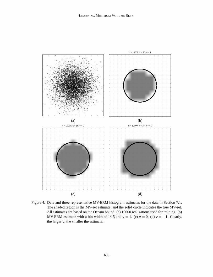
Figure 5 depicts the errorE (G) of the MV-SRM estimate withν = 1. The Occam’s Razorpenalty consistently outperforms the Rademacher penalty. For comparison,a damped version (ν =0) was also evaluated. It is clear from the graphs thatν = 0 outperformsν = 1. This happens becausethe damped version distributes the error more evenly between mass and volume, as discussed inSection 5.

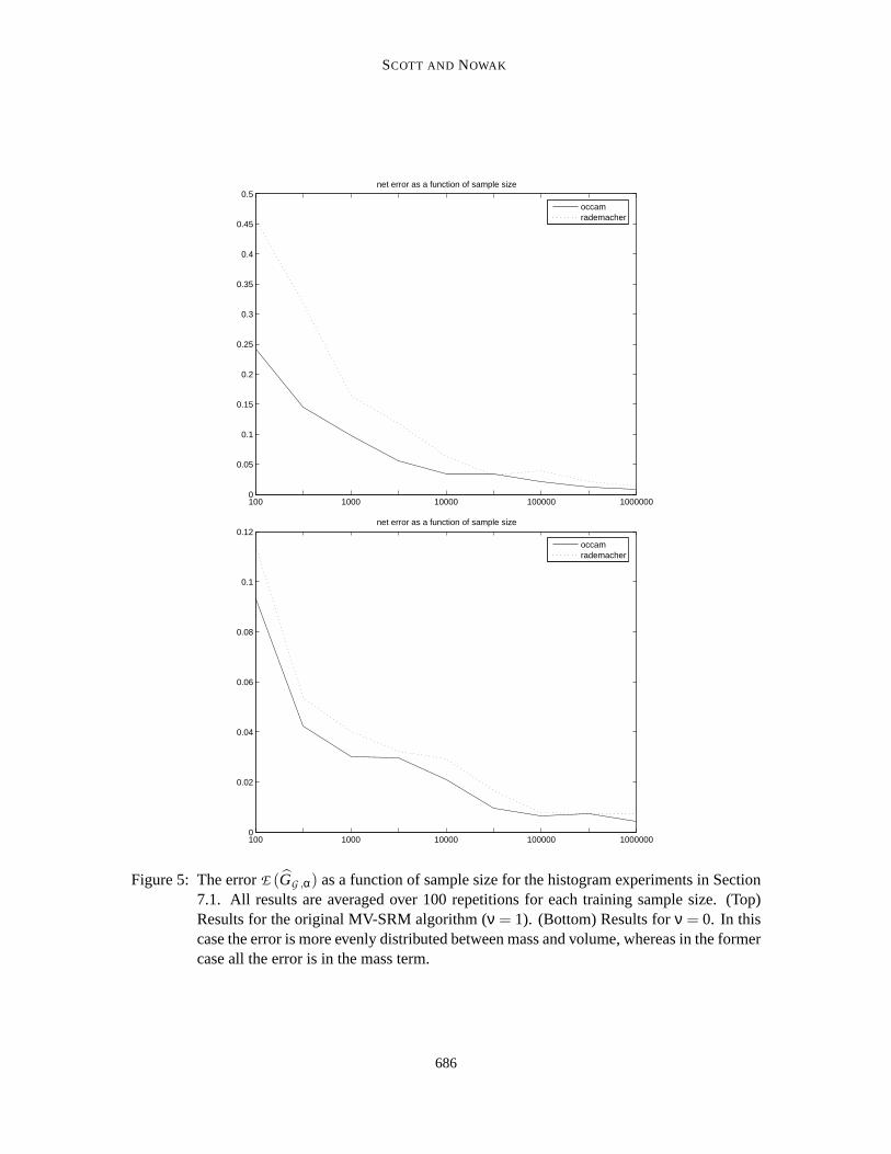
Figure 6 depicts the penalized volume of the MV-ERM estimates (ν = 1) as a function of theresolutionk, where 1/k is the sidelength of the histogram cell. MV-SRM selects the resolutionwhere this curve is minimized. Clearly the Occam’s Razor bound is tighter than the Rademacherbound (look at the right side of the graph), which explains why Occam outperforms Rademacher.Figure 7 depicts the average resolution of the estimate (top) and the averagesymmetric differencewith respect to the true MV-set, for various sample sizes. These graphs are for ν = 1. The graphsfor ν = 0 do not change considerably. Thus, while damping seems to have a noticeable effect on theerror quantityE , the effect on the symmetric difference is much less pronounced.

7.2 Dyadic Decision Trees

Implementing MV-SRM for dyadic decision trees is much more challenging than for histograms.Although an exact algorithm is possible (see Scott and Nowak, 2005a), we suggest an approximate

684

LEARNING M INIMUM VOLUME SETS

n = 10000, k = 15, ν = 1

(a) (b)n = 10000, k = 15, ν = 0 n = 10000, k = 15, ν = −1

(c) (d)

Figure 4: Data and three representative MV-ERM histogram estimates for the data in Section 7.1.The shaded region is the MV-set estimate, and the solid circle indicates the trueMV-set.All estimates are based on the Occam bound. (a) 10000 realizations used for training. (b)MV-ERM estimate with a bin-width of 1/15 andν = 1. (c) ν = 0. (d) ν = −1. Clearly,the largerν, the smaller the estimate.

685

SCOTT AND NOWAK

100 1000 10000 100000 10000000

0.05

0.1

0.15

0.2

0.25

0.3

0.35

0.4

0.45

0.5net error as a function of sample size

occamrademacher

100 1000 10000 100000 10000000

0.02

0.04

0.06

0.08

0.1

0.12net error as a function of sample size

occamrademacher

Figure 5: The errorE (GG ,α) as a function of sample size for the histogram experiments in Section7.1. All results are averaged over 100 repetitions for each training samplesize. (Top)Results for the original MV-SRM algorithm (ν = 1). (Bottom) Results forν = 0. In thiscase the error is more evenly distributed between mass and volume, whereasin the formercase all the error is in the mass term.

686

LEARNING M INIMUM VOLUME SETS

0 5 10 15 20 25 30 35 400.4

0.5

0.6

0.7

0.8

0.9

1

1.1

resolution parameter k

aver

age

pena

lized

vol

ume

of M

V−

ER

M s

olut

ion

10000 samples

occamrademacher

Figure 6: The penalized volume of the MV-ERM estimatesGkG ,α, as a function ofk, where 1/k is

the sidelength of the histogram cell. The results are for a sample size of 10000. Resultsrepresent an average over 100 repetitions. Clearly, the Occam’s razor bound is smallerthan the Rademacher penalty (look at the right side of the plot), to which we mayattributeits improved performance (see Figure 5).

687

SCOTT AND NOWAK

100 1000 10000 100000 10000002

4

6

8

10

12

14

sample size

aver

age

reso

lutio

n (1

/bin

wid

th)

of m

v−sr

m e

stim

ate

occamrademacher

100 1000 10000 100000 10000000.05

0.1

0.15

0.2

0.25

0.3

0.35

0.4symmetric difference as a function of sample size

occamrademacher

Figure 7: Results from the histogram experiments in Section 7.1. All results are averaged over 100repetitions for each training sample size, and are for the non-damped version of MV-SRM (ν = 1). (Top) Average value of the resolution parameterk (1/k = sidelength ofhistogram cells) as a function of sample size. (Bottom) Average value of the symmetricdifference between the estimated and true MV-sets. Neither graph changes significantlyif ν is varied.

688

LEARNING M INIMUM VOLUME SETS

algorithm based on a reformulation of the constrained optimization problem defining MV-SRM interms of its Lagrangian, coupled with a bisection search to find the appropriate Lagrange multiplier.If the penalty is additive, then the unconstrained Lagrangian can be minimizedefficiently usingexisting algorithmic approaches.

A penalty for a DDT is said to beadditiveif it can be written in the form

φ(GT) = ∑A∈π(T)

ψ(A)

for someψ. If φ is additive the optimization in (18) can be re-written as

minT∈T L

∑A∈π(T)

[µ(A)ℓ(A)+(1+ν)ψ(A)] subject to ∑A∈π(T)

[P(A)ℓ(A)+νψ(A)

]≥ α

whereℓ(A) is the binary label of leafA (ℓ(A) = 1 if A is in the candidate set and 0 otherwise). In-troducing the Lagrange multiplierλ > 0, the unconstrained Lagrangian formulation of the problemis

minT

∑A∈T

[µ(A)ℓ(A)+(1+ν)ψ(A)−λ

(P(A)ℓ(A)+νψ(A)

)].

Inspection of the Lagrangian reveals that the optimal choice ofℓ(A) is

ℓ(A) =

1 if λP(A) ≥ µ(A),

0 otherwise

Thus, we have a “per-leaf” cost function

cost(A) := min(µ(A)−λP(A),0)+(1+ν(1−λ))ψ(A)

For a given value ofλ, the optimal tree can be efficiently obtained using the algorithm of Blanchardet al. (2004).

We also note that the above strategy works for tree structures besides theone studied in Section6. For example, suppose an overfitted tree (with arbitrary, non-dyadic splits) has been constructedby some greedy heuristic (perhaps using an independent data set). Or,suppose that instead of binarydyadic splits with arbitrary orientation, one only considers “quadsplits” whereby every parent nodehas 2d children (in fact, this is the tree structure used for our experiments below).In such cases,optimizing the Lagrangian reduces to a classical pruning problem, and the optimal tree can be foundby a simpleO(n) dynamic program that has been used since at least the days of CART (Breimanet al., 1984).

Let Tλ denote the tree resulting from the Lagrangian optimization above. From standard opti-mization theory, we know that for each value ofλ, Tλ will coincide with Gα, for a certain value ofα. For each value ofλ there is a correspondingα, but the converse is not necessarily true. There-fore, the Lagrangian solutions correspond to many, but not all possiblesolutions of the originalMV-SRM optimization with different values ofα. Despite this potential limitation, the simplicity ofthe Lagrangian optimization makes this a very attractive approach to MV-SRM inthis case. We candetermine the best value ofλ for a given targetα by repeatedly solving the Lagrangian optimizationand finding the setting forλ that meets or comes closest to the original constraint. The search overλ can be conducted efficiently using a bisection search.

689

SCOTT AND NOWAK

In our experiments we do not consider the “free-split” tree structure described in Section 6, inwhich each parent has two children defined by one ofd = 2 possible splits. Instead, we assume aquadsplit tree structure, whereby every cell is a square, and every parent has four square children.The total optimization time isO(mn), wherem is the number of steps in the bisection search. In ourexperiments presented below we found that ten steps (i.e., ten Lagrangian tree pruning optimiza-tions) were sufficient to meet the constraint almost exactly (whenever possible).

We consider three complexity penalties. We refer to the first penalty as theminimaxpenalty,since it is inspired by the minimax optimal penalty in (19):

ψmm(A) := (0.01)

√

8max

(P(A),

JAK log2+ log(2/δ)

n

)JAK log2+ log(2/δ)

n. (23)

Note that the penalty is down-weighted by a constant factor of 0.01, since otherwise it is too largeto yield meaningful results:3

The second penalty is based on the Rademacher penalty (see Section 2.3).Let ΠL denote theset of all partitionsπ of trees inT L. Given π0 ∈ ΠL, setGπ0 = GT ∈ G L : π(T) = π0. Recallπ(T) denotes the partition associated with the treeT. Combining Proposition 7 with the results ofAppendix E, we know that for any fixedπ,

∑A∈π

√P(A)

n+

√2log(2/δ)

n

is a complexity penalty forGπ. To obtain a penalty for allG L = ∪π∈ΠLGπ, we apply the unionbound over allπ ∈ ΠL and replaceδ by δ|ΠL|−1. Although distributing the “delta” uniformly acrossall partitions is perhaps not intuitive (one might expect smaller partitions to be more likely andhence they should receive a larger chunk of the delta), it has the important property that the deltaterm is the same for all trees, and thus can be dropped for the purposes of minimization. Hence,the effective penalty is additive. In summary, our second penalty, referred to as the Rademacherpenalty,4 is given by

ψRad(A) =

√P(A)

n. (24)

The third penalty is referred to as the modified Rademacher penalty and is given by

ψmRad(A) =

√P(A)+µ(A)

n. (25)

The modified Rademacher penalty is still a valid penalty, since it strictly dominates the basicRademacher penalty. The basic Rademacher is proportional to the square-root of the empiricalP mass and the modified Rademacher is proportional to the square-root of thetotal mass (empirical

3. Note that here down-weighting is distinct from damping byν as discussed earlier. With down-weighting, bothoccurrences of the penalty, in the constraint and in the objective function, are scaled by the same factor. The oracleinequality (and hence minimax optimality) still holds for the downweighted penalty, albeit with larger constants.

4. Technically, this is an upper bound on the Rademacher penalty, but asdiscussed in Appendix E, this bound is tight towithin a factor of

√2. Using the exact Rademacher yields essentially the same results. Thus,we refer to this upper

bound simply as the Rademacher penalty.

690

LEARNING M INIMUM VOLUME SETS

P mass plusµ mass). In our experiments we have found that the modified Rademacher penaltytypically performs better than the basic Rademacher penalty, since it discourages the inclusion ofvery small isolated leafs containing a single data point (as seen in the experimental results below).Note that, unlike the minimax penalty, the two Rademacher-based penalties are not down-weighted;the true penalties are used.

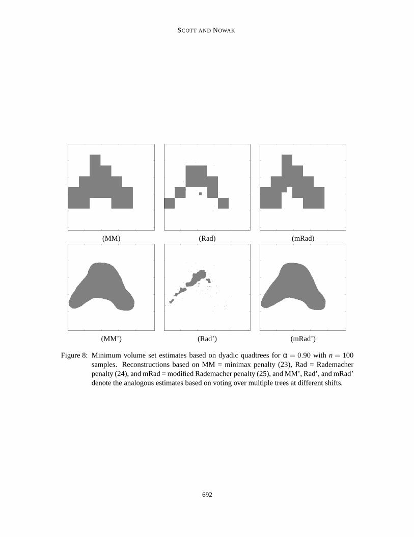
We illustrate the performance of the dyadic quadtree approach with a two-dimensional Gaus-sian mixture distribution, takingν = 0. Figure 1 depicts 500 samples from the Gaussian mixturedistribution, along with the true minimum volume set forα = 0.90. Figures 8, 9, and 10 depict theminimum volume set estimates based on each of the three penalties, and for samplesizes of 100,1000, and 10000. Here we use MM, Rad, and mRad to designate the three penalties.

In addition to the minimum volume set estimates based on a single tree, we also show theestimates based on voting over shifted partitions. This amounts to constructing 2L × 2L differenttrees, each based on a partition offset by an integer multiple of the base sidelength 2−L, and takinga majority vote over all the resulting set estimates to form the final estimate. Theseestimates areindicated by MM’, Rad’, and mRad’, respectively. Similar methods based onaveraging or votingover shifted partitions have been tremendously successful in image processing, and they tend tomitigate the “blockiness” associated with estimates based on a single tree, as is clearly seen in theresults depicted. Moreover, because of the significant amount of redundancy in the shifted partitions,the MM’, Rad’, and mRad’ estimates can be computed in justO(mnlogn) operations.

Visual inspection of the resulting minimum volume set estimates (which were “typical” resultsselected at random) reveals some of the characteristics of the different penalties and their behav-iors as a function of the sample size. Notably, the basic Rademacher penalty tends to allow verysmall and isolated leafs into the final set estimate, which is somewhat unappealing. The modifiedRademacher penalty clearly eliminates this problem and provides very reasonable estimates. The(down-weighted) minimax penalty results in set estimates quite similar to those resulting from themodified Rademacher. However, the somewhat arbitrary choice of scalingfactor (0.01 in this case)is undesirable. Finally, let us remark on the significant improvement provided by voting over multi-ple shifted trees. The voting procedure quite dramatically reduces the “blocky” partition associatedwith estimates based on single trees. Overall, the modified Rademacher penalty coupled with votingover multiple shifted trees appears to perform best in our experiments. In fact, in the casen= 10000,this set estimate is almost identical to the true minimum volume set depicted in Figure 1.

8. Conclusions

In this paper we propose two rules, MV-ERM and MV-SRM, for estimation ofminimum volumesets. Our theoretical analysis is made possible by relating the performance of these rules to theuniform convergence properties of the class of sets from which the estimate is taken. This in turnlets us apply distribution free uniform convergence results such as the VCinequality to obtaindistribution free, finite sample performance guarantees. It also leads to strong universal consistencywhen the class of candidate sets is allowed to grow in a controlled way. MV-SRM obeys an oracleinequality and thereby automatically selects the appropriate complexity of the setestimator. Thesetheoretical results are illustrated with histograms and dyadic decision trees.

Our estimators, results, and proof techniques for minimum volume sets bear a strong resem-blance to existing estimators, results, and proof techniques for supervised classification. This is nocoincidence. Minimum volume set estimation is closely linked with hypothesis testing.Assume

691

SCOTT AND NOWAK

(MM) (Rad) (mRad)

(MM’) (Rad’) (mRad’)

Figure 8: Minimum volume set estimates based on dyadic quadtrees forα = 0.90 with n = 100samples. Reconstructions based on MM = minimax penalty (23), Rad = Rademacherpenalty (24), and mRad = modified Rademacher penalty (25), and MM’, Rad’, and mRad’denote the analogous estimates based on voting over multiple trees at different shifts.

692

LEARNING M INIMUM VOLUME SETS

(MM) (Rad) (mRad)

(MM’) (Rad’) (mRad’)

Figure 9: Minimum volume set estimates based on dyadic quadtrees forα = 0.90 with n = 1000samples. Reconstructions based on MM = minimax penalty (23), Rad = Rademacherpenalty (24), and mRad = modified Rademacher penalty (25), and MM’, Rad’, and mRad’denote the analogous estimates based on voting over multiple trees at different shifts.

693

SCOTT AND NOWAK

(MM) (Rad) (mRad)

(MM’) (Rad’) (mRad’)

Figure 10: Minimum volume set estimates based on dyadic quadtrees forα = 0.90 withn = 10000samples. Reconstructions based on MM = minimax penalty (23), Rad = Rademacherpenalty (24), and mRad = modified Rademacher penalty (25), and MM’, Rad’, andmRad’ denote the analogous estimates based on voting over multiple trees at differentshifts.

694

LEARNING M INIMUM VOLUME SETS

P has a density with respect toµ, and thatµ is a probability measure. Then the minimum vol-ume set with massα is the acceptance region of the most powerful test of size 1−α for testingH0 : X ∼ P versus H1 : X ∼ µ. But classification and hypothesis testing have the same goals; thedifference lies in what knowledge is used to design a classifier/test (training data versus knowledgeof the true densities). The problem of learning minimum volume sets stands halfway between thesetwo: For one class the true distribution is known (the reference measure),but for the other onlytraining samples are available.

This observation provides not only intuition for the similarity between MV-set estimation andclassification, but it also suggests an alternative approach to MV-set estimation. In particular, sup-pose it is possible to sample at will from the reference measure. Consider these samples, togetherwith the original training data, to be a labeled training set. Then the MV-set may be estimated bylearning a classifier with respect to the Neyman-Pearson criterion (Cannon et al., 2002; Scott andNowak, 2005b). Briefly, the Neyman-Pearson classification paradigm involves learning a classi-fier from training data that minimizes the “miss” generalization error while constraining the “falsealarm” generalization error to be less than or equal to a specified size, in our case 1−α.

Minimum volume set estimation based on Neyman-Pearson classification offersa distinct ad-vantage over the rules studied in this paper. Indeed, our algorithms for histograms and dyadicdecision trees take advantage of the fact that the reference measureµ is easily evaluated for thesespecial types of sets. For more general sets or non-uniform reference measures, direct evaluationof the reference measure may be impractical. Neyman-Pearson classification, in contrast, involvescomputing the empirical volume based on the training sample, a much easier task. Moreover, inprinciple one may take an arbitrarily large sample fromµ to mitigate finite sample effects. A similaridea has been employed by Steinwart et al. (2005), who sample fromµ so as to reduce density levelset estimation to cost-sensitive classification. In this setting the advantage of MV-sets over densitylevel sets is further magnified. For example, to sample from a uniform distribution, one must specifyits support, which is a priori unknown. Fortunately, MV-sets are invariant to the choice of support,whereas theγ-level set changes with the support ofµ.

Acknowledgments

The authors thank Ercan Yildiz and Rebecca Willett for their assistance with the experiments in-volving dyadic trees, Gilles Blanchard for his insights into the Rademacher penalty for partition-based estimators, and an anonymous referee for suggesting a simplificationin the proof of Theorem10.

The first author was supported by an NSF VIGRE postdoctoral training grant. The secondauthor was supported by NSF Grants CCR-0310889 and CCF-0353079.

Appendix A. Proof of Lemma 4

The proof follows closely the proof of Lemma 1 in Cannon et al. (2002). DefineΞ = S: P(GG ,α) <

α−φ(GG ,α,S,δ). It is true thatΘµ ⊂ Ξ. To see this, ifS/∈ Ξ thenGG ,α ∈ Gα, and henceµ(GG ,α)≤µ(GG ,α) by definition ofGG ,α. ThusS /∈ Θµ. It follows that

ΘP∪Θµ ⊂ ΘP∪Ξ

695

SCOTT AND NOWAK

and hence it suffices to showΘP ⊂ ΩP andΞ ⊂ ΩP.First, we show thatΘP ⊂ ΩP. If S∈ ΘP then

P(GG ,α) < α−2φ(GG ,α,S,δ).

This implies

P(GG ,α)− P(GG ,α) < α−2φ(GG ,α,S,δ)− P(GG ,α)

≤ −φ(GG ,α,S,δ),

where the last inequality is true becauseP(GG ,α) ≥ α−φ(GG ,α,S,δ). ThereforeS∈ ΩP.Second, we show thatΞ ⊂ ΩP. If S∈ Ξ, then

P(GG ,α)−P(GG ,α) < α−φ(GG ,α,S,δ)−P(GG ,α)

≤ −φ(GG ,α,S,δ),

where the last inequality holds becauseP(GG ,α) ≥ α. Thus,S∈ ΩP, and the proof is complete.

Appendix B. Proof of Theorem 9

By the Borel-Cantelli Lemma (Durrett, 1991), it suffices to show that for any ε > 0,

∞

∑n=1

Pn(E (GG ,α) > ε) < ∞.

We will show this by establishing

∞

∑n=1

Pn((

µ(GG ,α)−µ∗α)

+>

ε2

)< ∞ (26)

and∞

∑n=1

Pn((

α−P(GG ,α))

+>

ε2.)

< ∞ (27)

First consider (26). By assumption (11), there existsK such thatµ(GkG ,α)−µ∗α ≤ ε/2 for all

k≥ K. Let N be such thatk(n) ≥ K for n≥ N. For any fixedn≥ N, consider a sampleSof sizen.By Theorem 3, it follows that with probability at least 1−δ(n), µ(GG ,α)−µ∗α ≤ µ(Gk

G ,α)−µ∗α ≤ ε/2.Therefore

∞

∑n=1

Pn((

µ(GG ,α)−µ∗α)

+>

ε2

)

=N−1

∑n=1

Pn((

µ(GG ,α)−µ∗α)

+>

ε2

)+

∞

∑n=N

Pn((

µ(GG ,α)−µ∗α)

+>

ε2

)

≤N−1

∑n=1

Pn((

µ(GG ,α)−µ∗α)

+>

ε2

)+

∞

∑n=N

δ(n)

< ∞.

696

LEARNING M INIMUM VOLUME SETS

The second inequality follows from the assumed summability ofδ(n).To establish (27), letN be large enough so that

supG∈G k(n)

φk(G,S,δ(n)) ≤ ε4

for all n≥ N. For any fixedn≥ N, consider a sampleSof sizen. By Theorem 3, it follows that withprobability at least 1−δ(n), α−P(GG ,α) ≤ 2φk(GG ,α,S,δ(n)) ≤ ε/2. Therefore

∞

∑n=1

Pn((

α−P(GG ,α))

+>

ε2

)

=N−1

∑n=1

Pn((

α−P(GG ,α))

+>

ε2

)+

∞

∑n=N

Pn((

α−P(GG ,α))

+>

ε2

)

≤N−1

∑n=1

Pn((

α−P(GG ,α))

+>

ε2

)+

∞

∑n=N

δ(n)

< ∞.

This completes the proof.

Appendix C. Proof of Theorem 10

The first part of the theorem is straightforward. First, we claim that(µ(Gn)−µ∗α)+ ≤ µ(Gn\G∗α). To

see this, assumeµ(Gn)−µ∗α ≥ 0, otherwise the statement is trivial. Then

(µ(Gn)−µ∗α)+ = µ(Gn)−µ∗α= µ(Gn)−µ(G∗

α)

≤ µ(Gn)−µ(G∗α ∩Gn)

= µ(Gn\G∗α).

Similarly, one can show(α−P(Gn))+ ≤ P(G∗α\Gn). Let Dγ = x : f (x) ≥ γ andEn = G∗

α\Gn.Then for anyγ > 0,

P(En) = P(En∩Dγ)+P(En∩Dγ) ≤ P(Dγ)+ γµ(En).

By the dominated convergence theorem,P(Dγ) → 0 asγ → ∞. Thus, for anyε > 0, we can chooseγ such thatP(Dγ) ≤ ε and thenn large enough so thatγµ(En) ≤ ε. The result follows.

Now the second part of the theorem. From Section 1.2, we knowG∗α = x : f (x) = γα where

γα is the unique number such thatR

f (x)≥γαf (x)dµ(x) = α.

Consider the distributionQ of (X,Y) ∈ X ×0,1 given by the class-conditional distributionsX|Y = 0∼ P andX|Y = 1∼ µ, and a priori class probabilitiesQ(Y = 0) = p= 1−Q(Y = 1), wherep will be specified below. ThenQ defines a classification problem. Leth∗ denote a Bayes classifierwith respect toQ (i.e., a classifier with minimum probability of error), and leth : X → 0,1 be anarbitrary classifier. The classification risk ofh is defined asR (h) = Q(h(X) 6= Y), and the excessclassification risk isR (h)−R (h∗). From Bayes decision theory we know thath∗ is the rule thatcompares the likelihood ratio top/(1− p). But, as discussed in Section 1.2, the likelihood ratio is1/ f . Therefore, ifp is such thatp/(1− p) = 1/γα, thenh∗(x) = 1−I(x∈ G∗

α) µalmost everywhere.

697

SCOTT AND NOWAK

Settinghn(x) = 1− I(x∈ Gn), we have

R (hn)−R (h∗)

= Q(hn(X) 6= Y)−Q(h∗(X) 6= Y)

= (1− p)(µ(hn(X) = 0)−µ(h∗(X) = 0)))+ p(P(hn(X) = 1)−P(h∗(X) = 0))

= (1− p)(µ(Gn)−µ(G∗α))+ p(1−P(Gn)− (1−P(G∗

α)))

= (1− p)(µ(Gn)−µ∗α)+ p(α−P(Gn))

≤ (µ(Gn)−µ∗α)+(α−P(Gn))

≤ E (Gn).

ThereforeR (hn) → R (h∗). We now invoke a result of Steinwart et al. (2005) that says, in ournotation, thatR (hn) → R (h∗) if and only if µ(Gn∆G∗

α) → 0, and the proof is complete.

Appendix D. Proof of Theorem 11

Let ΩP be as in the proof of Theorem 3, and assumeS∈ ΩP. This holds with probability at least1−δ. We consider three separate cases: (1)µ(GG ,α) ≥ µ∗α andP(GG ,α) < α, (2) µ(GG ,α) ≥ µ∗α and

P(GG ,α)≥α, and (3)µ(GG ,α) < µ∗α andP(GG ,α) < α. Note that the case in which bothα≤P(GG ,α)

andµ(GG ,α) < µ∗α is impossible by definition of minimum volume sets. We will use the followingfact:

Lemma 17 If S∈ ΩP, thenα−P(GG ,α) ≤ 2φ(GG ,α,S,δ).

The proof is a repetition of the proof thatΘP ⊂ ΩP in Lemma 4.For the first case we have

E (GG ,α) = µ(GG ,α)−µ∗α +α−P(GG ,α)

≤ µ(GG ,α)−µ∗α +2φ(GG ,α,S,δ)

= infG∈Gα

µ(G)−µ∗α +2φ(G,S,δ)

≤ infG∈Gα

µ(G)−µ∗α +2φ(G,S,δ)

≤(

1+1γα

)inf

G∈Gα

µ(G)−µ∗α +2φ(G,S,δ)

.

The first inequality follows fromS∈ ΘP. The next line comes from the definition ofGG ,α. The

second inequality follows fromS∈ ΩP, from which it follows thatGα ⊂ Gα. The final step is trivial(this constant is needed for case 3).

For the second case,µ(GG ,α) ≥ µ∗α andP(GG ,α) ≥ α, note

E (GG ,α) = µ(GG ,α)−µ∗α

≤ µ(GG ,α)−µ∗α +2φ(GG ,α,S,δ)

698

LEARNING M INIMUM VOLUME SETS

and proceed as in the first case.For the third case,µ(GG ,α) < µ∗α andP(GG ,α) < α, we rely on the following lemmas.

Lemma 18 Let ε > 0. Thenµ∗α −µ∗α−ε ≤

εγα

.

Proof By assumptionsA1 andA2, there exist MV-setsG∗α−ε andG∗

α such that

Z

G∗α

f (x)dµ(x) = α

andZ

G∗α−ε

f (x)dµ(x) = α− ε.

Furthermore, we may chooseG∗α−ε andG∗

α such thatG∗α−ε ⊂ G∗

α. Thus

ε =Z

G∗α

f (x)dµ(x)−Z

G∗α−ε

f (x)dµ(x)

=Z

G∗α\G∗

α−ε

f (x)dµ(x)

≥ γαµ(G∗α\G∗

α−ε)

= γα(µ∗α −µ∗α−ε)

and the result follows.

Lemma 19 If S∈ ΩP and G∈ Gα, then

µ∗α −µ(G) ≤ 2γα

·φ(G,S,δ).

Proof Denoteε = 2φ(G,S,δ). SinceS∈ ΩP andG∈ Gα, we know

P(G) ≥ P(G)− 12

ε ≥ α− ε.

In other words,G∈ Gα−ε. Therefore,µ(G) ≥ µ∗α−ε and it suffices to boundµ∗α −µ∗α−ε. Now applythe preceding lemma.

699

SCOTT AND NOWAK

It now follows that

E (GG ,α) = α−P(GG ,α)

≤ 2φ(GG ,α,S,δ)

= µ(GG ,α)−µ∗α +µ∗α −µ(GG ,α)+2φ(GG ,α,S,δ)

≤ µ(GG ,α)−µ∗α +

(1+

1γα

)2φ(GG ,α,S,δ)

≤(

1+1γα

)(µ(GG ,α)−µ∗α +2φ(GG ,α,S,δ)

)

=

(1+

1γα

)inf

G∈Gα

µ(G)−µ∗α +2φ(G,S,δ)

≤(

1+1γα

)inf

G∈Gα

µ(G)−µ∗α +2φ(G,S,δ)

The first inequality follows from Lemma 17. The second inequality is by Lemma 19. The next tolast line follows from the definition ofGG ,α, and the final step is implied byS∈ ΩP as in case 1.This completes the proof.

Appendix E. The Rademacher Penalty for Partition-Based Sets

In this appendix we show how the conditional Rademacher penalty introducedin Section 2.3 can beevaluated for a classG based on a fixed partition. The authors thank Gilles Blanchard for pointingout the properties that follow. Letπ = A1, . . . ,Ak be a fixed, finite partition ofX , and letG be theset of all sets formed by taking the union of cells inπ. Thus|G | = 2k and everyG∈ G is specifiedby ak-length string of binary digitsℓ(A1), . . . , ℓ(Ak), with ℓ(A) = 1 if and only ifA⊂ G.

The conditional Rademacher penalty may be rewritten as follows:

2n

E(σi)

[supG∈G

n

∑i=1

σiI(Xi ∈ G)

]=

2n

E(σi)

[sup

ℓ(A) :A∈π

n

∑i=1

σiℓ(A)

]

=2n ∑

A∈πE(σi)

[supℓ(A)

∑i:Xi∈A

σiℓ(A)

]

=: ∑A∈π

ψ(A).

700

LEARNING M INIMUM VOLUME SETS

Thus the penalty is additive (modulo the delta term). Now consider a fixed cellA:

ψ(A) =2n

E(σi)

[supℓ(A)

∑i:Xi∈A

σiℓ(A)

]

=1n

E(σi)

[supℓ(A)

∑i:Xi∈A

σi(2ℓ(A)−1)

]

=1n

E(σi)

[supℓ(A)

(2ℓ(A)−1) ∑i:Xi∈A

σi

]

=1n

E(σi)

[∣∣∣∣∣ ∑i:Xi∈A

σi

∣∣∣∣∣

].

Now let bin(M, p,m) =(M

m

)pm(1− p)M−m be the probability of observingmsuccesses in a sequence

of M Bernoulli trials having success probabilityp. Then this last expression can be computedexplicitly as

ψ(A) =1n

nA

∑i=0

bin(nA,1/2, i)|nA−2i|,

wherenA = |i : Xi ∈ A|. This is the penalty used in the histogram experiments (after the delta termis included).

A more convenient and intuitive penalty may be obtained by bounding

ψ(A) =1n

E(σi)

[∣∣∣∣∣ ∑i:Xi∈A

σi

∣∣∣∣∣

]

≤ 1n

E(σi)

(

∑i:Xi∈A

σi

)2

12

=1n

E(σi)

[

∑i:Xi∈A

σ2i

] 12

=

√P(A)

n,

where the inequality is Jensen’s. Moreover, by the Khinchin-Kahane inequality (see, e.g., Ledouxand Talagrand, 1991, Lemma 4.1), the converse inequality holds with a factor

√2, so the bound

is tight up to this factor. This is the “Rademacher” penalty employed in the dyadicdecision treeexperiments.

References

A. Baillo, J. A. Cuesta-Albertos, and A. A. Cuevas. Convergence rates in nonparametric estimationof level sets.Stat. Prob. Letters, 53:27–35, 2001.

P. Bartlett, S. Boucheron, and G. Lugosi. Model selection and error estimation. Machine Learning,48:85–113, 2002.

701

SCOTT AND NOWAK

S. Ben-David and M. Lindenbaum. Learning distributions by their density levels: a paradigm forlearning without a teacher.J. Comp. Sys. Sci., 55:171–182, 1997.

G. Blanchard, C. Schafer, and Y. Rozenholc. Oracle bounds and exact algorithm for dyadic classifi-cation trees. In J. Shawe-Taylor and Y. Singer, editors,Learning Theory: 17th Annual Conferenceon Learning Theory, COLT 2004, pages 378–392. Springer-Verlag, Heidelberg, 2004.

O. Bousquet, S. Boucheron, and G. Lugosi. Introduction to statistical learning theory. In O. Bous-quet, U.v. Luxburg, and G. Rtsch, editors,Advanced Lectures in Machine Learning, pages 169–207. Springer, 2004.

L. Breiman, J. Friedman, R. Olshen, and C. Stone.Classification and Regression Trees. Wadsworth,Belmont, CA, 1984.

A. Cannon, J. Howse, D. Hush, and C. Scovel. Learning with the Neyman-Pearson and min-maxcriteria. Technical Report LA-UR 02-2951, Los Alamos National Laboratory, 2002. URLhttp://www.c3.lanl.gov/∼kelly/ml/pubs/2002 minmax/paper.pdf.

A. Cohen, W. Dahmen, I. Daubechies, and R. A. DeVore. Tree approximation and optimal encoding.Applied and Computational Harmonic Analysis, 11(2):192–226, 2001.

T. Cover and J. Thomas.Elements of Information Theory. John Wiley and Sons, New York, 1991.

A. Cuevas and R. Fraiman. A plug-in approach to support estimation.Ann. Stat., 25:2300–2312,1997.

A. Cuevas and A. Rodriguez-Casal. Set estimation: An overview and somerecent developments.Recent advances and trends in nonparametric statistics, pages 251–264, 2003.

R. A. DeVore. Nonlinear approximation.Acta Numerica, 7:51–150, 1998.

L. Devroye, L. Gyorfi, and G. Lugosi.A Probabilistic Theory of Pattern Recognition. Springer,New York, 1996.

D. Donoho. Wedgelets: Nearly minimax estimation of edges.Ann. Stat., 27:859–897, 1999.

R. Durrett. Probability: Theory and Examples. Wadsworth & Brooks/Cole, Pacific Grove, CA,1991.

J. Hartigan. Estimation of a convex density contour in two dimensions.J. Amer. Statist. Assoc., 82(397):267–270, 1987.

X. Huo and J. Lu. A network flow approach in finding maximum likelihood estimateof highconcentration regions.Computational Statistics and Data Analysis, 46(1):33–56, 2004.

J. Klemela. Complexity penalized support estimation.J. Multivariate Anal., 88:274–297, 2004.

V. Koltchinskii. Rademacher penalties and structural risk minimization.IEEE Trans. Inform. The-ory, 47:1902–1914, 2001.

J. Langford. Tutorial on practical prediction theory for classification.J. Machine Learning Research,6:273–306, 2005.

702

LEARNING M INIMUM VOLUME SETS

M. Ledoux and M. Talagrand.Probability in Banach spaces. Springer-Verlag, Berlin, 1991.

G. Lugosi and K. Zeger. Concept learning using complexity regularization. IEEE Trans. Inform.Theory, 42(1):48–54, 1996.

G. Lugosi and K. Zeger. Nonparametric estimation using empirical risk minimization. IEEE Trans.Inform. Theory, 41(3):677–687, 1995.

D. Muller and G Sawitzki. Excess mass estimates and tests for multimodality.J. Amer. Statist.Assoc., 86(415):738–746, 1991.

A. Munoz and J. M. Moguerza. Estimation of high-density regions using one-class neighbor ma-chines.IEEE Trans. Patt. Anal. Mach. Intell., 28:476–480, 2006.

D. Nolan. The excess mass ellipsoid.J. Multivariate Analysis, 39:348–371, 1991.

J. Nunez-Garcia, Z. Kutalik, K.-H.Cho, and O. Wolkenhauer. Level sets and minimum volume setsof probability density functions.Approximate Reasoning, 34:25–47, Sept. 2003.

W. Polonik. Measuring mass concentrations and estimating density contour cluster–an excess massapproach.Ann. Stat., 23(3):855–881, 1995.

W. Polonik. Minimum volume sets and generalized quantile processes.Stochastic Processes andtheir Applications, 69:1–24, 1997.

T. W. Sager. An iterative method for estimating a multivariate mode and isopleth.J. Am. Stat. Asso.,74:329–339, 1979.

B. Scholkopf, J. Platt, J. Shawe-Taylor, A. Smola, and R. Williamson. Estimating the support of ahigh-dimensional distribution.Neural Computation, 13(7):1443–1472, 2001.

C. Scott and R. Nowak. Learning minimum volume sets. Technical Report ECE-05-2, UW-Madison, 2005a. URLhttp://www.stat.rice.edu/∼cscott.

C. Scott and R. Nowak. A Neyman-Pearson approach to statistical learning. IEEE Trans. Inform.Theory, 51(8):3806–3819, 2005b.

C. Scott and R. Nowak. Minimax-optimal classification with dyadic decision trees. IEEE Trans.Inform. Theory, pages 1335–1353, April 2006.

I. Steinwart, D. Hush, and C. Scovel. A classification framework for anomaly detection.J. MachineLearning Research, 6:211–232, 2005.

A. B. Tsybakov. On nonparametric estimation of density level sets.Ann. Stat., 25:948–969, 1997.

V. Vapnik. Estimation of Dependencies Based on Empirical Data. Springer-Verlag, New York,1982.

V. Vapnik. Statistical Learning Theory. Wiley, New York, 1998.

R. Vert and J.-P. Vert. Consistency and convergence rates of one-class SVM and related algorithms.Technical Report 1414, Universit Paris-Sud, 2005.

703

SCOTT AND NOWAK

G. Walther. Granulometric smoothing.Ann. Stat., 25:2273–2299, 1997.

R. Willett and R. Nowak. Minimax optimal level set estimation. submitted toIEEE Trans. ImageProc., 2006. URLhttp://www.ee.duke.edu/∼willett/.

R. Willett and R. Nowak. Minimax optimal level set estimation. InProc. SPIE, Wavelets XI, 31July - 4 August, San Diego, CA, USA, 2005.

704