learning in repeated public goods games - a meta … · the experimental data is split into 18...
TRANSCRIPT
Learning in Repeated Public Goods Games - A MetaAnalysis
Chenna Reddy Cotla∗
December 2015
Abstract
I examine the generalizability of a broad range of prominent learning models in ex-plaining contribution patterns in repeated linear public goods games. Experimentaldata from twelve previously published papers is considered in testing several learn-ing models in terms of how accurately they describe individuals’ round-by-roundchoices. The experimental data is split into 18 datasets. Each of these datasets isdifferent from the remaining in at least one of the following aspects: the marginalper capita return, group size, matching protocol, number of rounds, and endowmentthat determines the number of stage game strategies. Both ex-post descriptive fit oflearning models and their ex-ante predictive accuracy are examined. The followinglearning models are included in the study: reinforcement learning, normalized rein-forcement learning, reinforcement average model with loss aversion strategy (REL),stochastic fictitious play, normalized stochastic fictitious play, experience weightedattraction learning (EWA), self-tuning EWA, and Impulse matching learning. RELoutperforms all other learning models in both within dataset descriptive fit and out-of-sample dataset predictive accuracy. While all the learning models out-performthe random choice benchmark, only REL performs at least as well as the model thatreflects dataset level overall empirical frequencies. The results suggest that learningin repeated linear public goods games is more in line with reinforcement learningthan that of belief learning or regret-based learning. Finally, REL also outperformsindividual evolutionary learning (IEL) in predicting the full distribution of contri-butions. Average reinforcement learning that is sensitive to the observed payoffvariability and insensitive to the payoff magnitude underlie the success of REL inexplaining contributions in repeated public goods games over a broad spectrum ofgame parameters.
JEL Codes: C63, C92, D83, H41Keywords: public goods games, learning, reinforcement learning, belief learning
∗Interdisciplinary Center for Economic Science and Department of Computational Social Science,George Mason University, Fairfax, VA 22030, email: [email protected]
1 Introduction
In this paper, I use data from controlled lab experiments and standard econometricmethods to compare a number of competing behavioral specifications of agents that arespecified as different learning models in the context of repeated public goods games.
A handful of earlier studies have used data from laboratory experiments on publicgoods games to test competing learning models (Cooper & Stockman, 2002; Janssen &Ahn, 2006; Arifovic & Ledyard, 2012; Wunder, Suri, & Watts, 2013). However, the ap-proaches used in these studies have limitations in terms of model generalizability eitherdue to the data used or the set of learning models considered or both. Cooper and Stock-man (2002) use the cumulative reinforcement learning model of Roth and Erev (1995) tomodel learning behavior in step level public goods games. They have used the data fromtheir own experiments to fit the model and derive conclusions. Previous research showsthat cumulative reinforcement learning is outperformed by average reinforcement learn-ing in predicting behavior (Erev & Roth, 1998; Ho, Camerer, & Chong, 2007). Arifovicand Ledyard (2012) and Janssen and Ahn (2006) consider data from multiple experi-ments conducted by Mark Isaac and his coauthors in studying learning in public goodsgames. However, similar to Cooper and Stockman (2002), they also considered only onelearning algorithm in their studies. The former exclusively considers their own IndividualEvolutionary Learning (IEL) model while the latter considers only Experience WeightedAttraction (EWA) learning model of Camerer and Ho (1999). Both of these papers, ex-amine learning models in terms of their within sample descriptive fit.Thus, these analysesare subject to the potential problem of model overfitting. Wunder et al. (2013) considera number of learning models, however, they take a purely machine learning approach byconsidering models that are difficult to interpret from the cognitive plausibility perspec-tive. Furthermore, they consider data from the experiments conducted in Suri and Watts(2011) and Wang, Suri, and Watts (2012) which involve public goods game with only oneset of game parameters. While their stochastic discounted two-factor model does verywell in both descriptive fit and predictive accuracy compared to a number of other learn-ing models considered in their paper, it is unclear if the model will also be successful inexplaining behavior in public goods games with different values for the game parameterslike the endowment, marginal return, number of rounds, and matching. This is a validconcern since previous studies have supported different models of learning in differentgames and the relationship among distinct conclusions obtained in different studies isoften not clear (Erev & Haruvy, 2013). Therefore, it remains an open question if anyof the models that were considered in these earlier studies are general enough to explainbehavior in public goods environments with wide ranging parameters.
The obstacles faced in understanding the learning mechanism individuals use in re-peated public goods environment, or for that matter in any repeated strategic environ-ment, using data from experiments can be listed as follows:
1. Small datasets due to the small number of experimental subjects: Smallsized data sets due to the small number of experimental subjects can induce selec-tion biases in econometric investigations. Often, datasets that are generated using
1
controlled lab experiments contain individuals in sub hundreds. They may not haveenough variation to compare competing learning models. Furthermore, an experi-mental dataset considered in isolation may consist of individuals drawn from a verynarrow spectrum of the population. Thus, a model that is favored by a single dataset may not generalize over.
2. Small number of rounds of in repeated games: Small number of rounds couldpotentially lead to misleading conclusions regarding which learning model performsbest. Learning models generally require sufficiently large number of rounds beforelearning process unfolds. When there are data for only a couple of rounds learningmodels’ performance could depend strongly on initial conditions. Different learningmodels could be made favorites by cleverly choosing suitable initial conditions.
3. The problem of model overfitting: Salmon (2001) and Hopkins (2002) haveshown that learning models can be very easily overfitted to the experimental data.The problem of overfitting is exacerbated when one is dealing with small data setsizes and a small set of learning models (Erev, Ert, & Roth, 2010).
4. Consideration of a relatively small set of models: Since every learning modelis a simplified representation of an underlying cognitive or neural mechanism, itis fair to say each of them is misspecified. If one considers only a very smallset of learning models, it is difficult to get a relative sense of what constitutes agood learning description in a given environment. Therefore, the choice of the setof learning models that one chooses to study can influence what conclusions onereaches. This point can also be demonstrated using the results in this paper. Ifone considered only belief learning models, one could potentially argue, using theresults in this paper, that learning does not perform better than a random choicemodel and thus is not useful in predicting behavior in public goods environments.By considering a large set of learning models that span across different families oflearning, one can reduce the potential model selection bias.
5. Choice of model comparison metric: The choice of a metric that one uses tocompare the performance of different learning models can potentially influence theconclusion one reaches. Feltovich (2000) studies the performance of reinforcementand belief learning models in the context of multi stage asymmetric informationgames. When he compares models using maximum log-likelihood achieved by them,a belief learning model outperforms a set of other models that includes a reinforce-ment learning model. However, when he considers Mean Squared Deviation (MSD)as the comparison metric, the reinforcement learning model outperforms the belieflearning model. In the work of Chmura, Goerg, and Selten (2012), the authors findthat impulse matching learning outperforms a number of other models in replicatingaggregate frequencies of observed choices, but, self-tuning EWA performs the bestin predicting individuals’ round-by-round behavior in twelve 2 × 2 games. Thus,the choice of comparison metric can have significant influence on the conclusionsone reaches.
2

In this paper I address these obstacles in understanding learning in public goods gamesby:
1. Considering a large dataset involving 1201 individuals and 17250 decisions thatis constructed using the experimental data from 12 different published studies.These studies are conducted with subjects from different nations, educational back-grounds, and are conducted by different researchers. This reduces the potentialdata selection bias in my investigation. As Erev and Roth (1998) states, there isdanger that researchers treat the models they propose as their toothbrushes, byusing one’s model on one’s own data. Experimenters may also unconsciously makesome decisions in their experimental design that could favor some learning modelsover others. My study seeks to overcome this danger by considering data frommultiple experiments.
2. Considering data on public goods games that involve at least 10 rounds of play andthus sufficiently allowing the learning process to unfold.
3. Comparing models using both descriptive fit and prediction accuracy. I dividethe experimental data on 1201 individuals into 18 separate datasets each of whichinvolves a public goods game with a unique set of game parameters. I comparehow generalizable each learning model is in two ways. First, using the parameterestimates of each learning model estimated from the pooled data of 1201 individuals,I test how well the same parameters explain behavior across datasets with varyingparameters of the game. Second, for each dataset I predict choices in it usingeach learning model with parameters estimated using the remaining 17 datasets. Icompare models based on how well they do in the prediction task. In both of thesecomparisons testing the generalizability of models, I use only non-parametric exacttests.
4. Considering nine learning models that cover a broad spectrum of types of learning.The following learning models are considered to model individual level adaptivebehavior: reinforcement learning (RL), normalized reinforcement learning (NRL),reinforcement average model with loss aversion strategy (REL), stochastic ficti-tious play (SFP), normalized stochastic fictitious play (NFP), experience weightedattraction learning (EWA), self-tuning EWA (STEWA), Impulse matching learning(IM), and Individual Evolutionary Learning (IEL). These models cover the ideasof reinforcement learning, belief learning, regret-based learning, hybrid learningthat incorporate elements from both belief and reinforcement learning, and individ-ual evolutionary learning. This choice of wide ranging models, helps to minimizemethodological bias that can enter into the analysis due to the consideration of avery narrow set (often of size one or two) of learning models.
5. Using a wide ranging comparison metrics in analyzing the effectiveness of learningmodels in replicating the observed behavior in the data. I consider log-likelihood(LL), Akaike Information Criterion (AIC), Bayesian Information Criterion (BIC),
3
and Mean Quadratic Score (MQS)1 achieved by learning models in comparing theirdescriptive fit and prediction accuracy. I also compare the most successful modelREL with the evolutionary learning model IEL using the distance between theobserved and predicted distribution of choices.
The main finding in this study is that REL outperforms all other learning models interms of both descriptive fit and prediction accuracy. It is the only model to outperformdataset level overall empirical frequencies in both descriptive fit and predictive accuracywhen model performance is compared using MQS. In terms of LL and BIC, REL performsas well as the empirical frequencies in both comparisons. None of the remaining modelsoutperform the empirical frequencies in both comparisons according to any of the metrics.EWA and NRL jointly take the second place. They are outperformed by the dataset levelempirical frequencies in terms of LL and BIC. But, they do as well as the dataset levelempirical frequencies in terms of MQS. The ordering of learning models in both compar-isons is identical: REL, NRL, EWA, RL, NSFP, SFP, IM, STEWA (the ordering is notstrict in all cases. REL performs strictly better than all other models). Belief learningmodels and regret-learning models perform poorly in comparison to reinforcement mod-els. In public goods environments, learning is more in line with reinforcement learning.Average reinforcement learning that is adaptive to observed payoff variability and insen-sitive to the payoff magnitude underlies the success of REL. REL also outperforms IELin predicting full distribution of contributions across all data sets.
The paper is organized as follows. In Section 2, I describe the linear public goodsenvironment. Section 3 describes the data that is used in econometric investigations.Section 4 presents a brief description of learning models. Section 5 presents results. Abrief discussion is presented in Section 6. Section 7 concludes the paper by summing upthe findings and discussing future directions.
2 Linear Public Goods Game
Before I proceed to the data and learning models that are considered in my analysis, I firstbriefly describe the linear public goods environment. A linear public good game consistsof Ng individuals. Index these individuals as i = 1, 2, .., Ng. Each individual is endowedwith an amount wi and must decide how much to contribute to the public good fromhis endowment and how much he wants to keep to himself. In this paper, I study publicgoods games where each individual is endowed with the same amount wi = E,∀i. Say anindividual’s contribution is denoted as ci ∈ [0, E], then his payoff from his contributiondecision is given as:
πi = E − ci +M
Ng∑j=1
cj
1Note that MQS is equivalent to Mean Squared Deviation (MSD) by an affine transformation. MQS= 1 - MSD for one dimensional distributions.
4
Where M is the marginal per capita return (MPCR) from the public good. As longas 1
Ng< M < 1, it is individually rational to contribute nothing to the public good but
the social optimum is achieved when everybody contributes their entire endowment. Inthis way, a linear public goods game epitomizes the tension between private and publicinterests that is the basis of any standard social dilemma.
In a repeated game, the stage described above is repeated over T number of rounds.In a finitely repeated game, the number of rounds, T , is determined beforehand. It is easyto see that zero contribution in each round is individually rational in a finitely repeatedpublic goods game.
3 Data
A number of published studies involving repeated public goods game experiments withat least 10 rounds were considered for data collection. Since the main aim of this study isto evaluate different learning models in terms of their descriptive and predictive power inexplaining choices over time, I considered only the baseline studies where no additionalmechanism like punishment was in place. For the studies where the data was not publiclymade available at the time of data collection, data was requested from the correspondingauthors. Data was obtained for experiments conducted in the following twelve publishedstudies: Andreoni (1988, 1995b, 1995a); Isaac and Walker (1988); Isaac, Walker, andWilliams (1994); Fehr and Gachter (2000); Nikiforakis and Normann (2008); Gachter,Renner, and Sefton (2008); Sefton, Shupp, and Walker (2007); Kosfeld, Okada, and Riedl(2009); Botelho, Harrison, Pinto, and Rutstrom (2009); Keser and Van Winden (2000).While a few more studies had data on baseline repeated public goods games of length 10or more rounds, the data was not readily available at the time of this study.
The experimental data from 12 published papers under consideration is reorganizedinto 18 datasets. Data from identical treatments across studies is combined and put intoa single dataset to obtain 18 distinct datasets that are different from each other in termsof at least one parameter of the public goods game itself. The parameters of the gamethat are used to distinguish among datasets are: the number of rounds of the repeatedgame (T ), group size (Ng), endowment (E), marginal per capita return (M), and matchingprotocol. The matching protocol can be Partners, Strangers, or Perfect Strangers. InPartners matching, group composition stays fixed over the rounds of a repeated game. InStrangers’ matching, groups are reshuffled in each round using the subject pool a givenexperimental session. However, Strangers’ matching does not guarantee that any twosubjects will not be matched more than once over the rounds of a repeated game. PerfectStrangers’ matching is identical to the Strangers’ matching except that it ensures thatno two subjects will be matched more than once over the rounds of a repeated game.Table 1 presents 18 datasets that are constructed from the data obtained from publishedstudies. No two datasets contain the same individual. These datasets cover a broad rangeof game parameters. For example, E ranges from 6 to 60, M varies between 0.03 to 0.8,Ng varies between 3 to 40, T ranges from 10 to 50. All three matching protocols areobserved across the datasets.
5
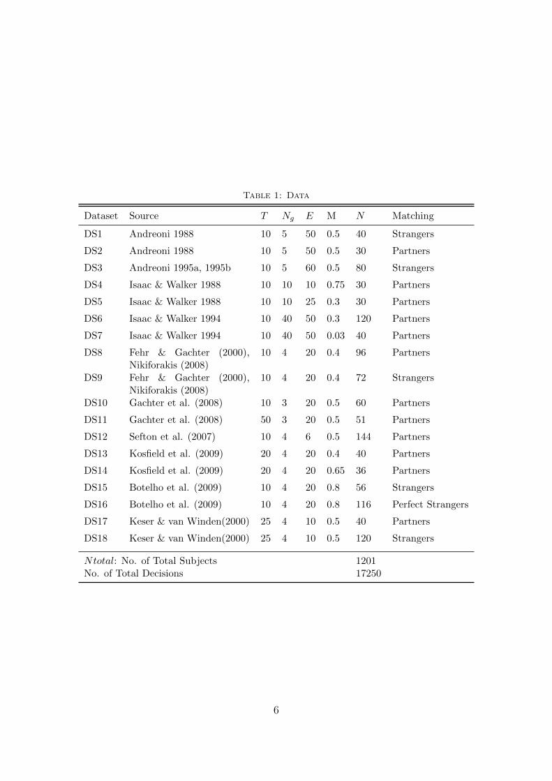
Table 1: Data
Dataset Source T Ng E M N Matching
DS1 Andreoni 1988 10 5 50 0.5 40 Strangers
DS2 Andreoni 1988 10 5 50 0.5 30 Partners
DS3 Andreoni 1995a, 1995b 10 5 60 0.5 80 Strangers
DS4 Isaac & Walker 1988 10 10 10 0.75 30 Partners
DS5 Isaac & Walker 1988 10 10 25 0.3 30 Partners
DS6 Isaac & Walker 1994 10 40 50 0.3 120 Partners
DS7 Isaac & Walker 1994 10 40 50 0.03 40 Partners
DS8 Fehr & Gachter (2000),Nikiforakis (2008)
10 4 20 0.4 96 Partners
DS9 Fehr & Gachter (2000),Nikiforakis (2008)
10 4 20 0.4 72 Strangers
DS10 Gachter et al. (2008) 10 3 20 0.5 60 Partners
DS11 Gachter et al. (2008) 50 3 20 0.5 51 Partners
DS12 Sefton et al. (2007) 10 4 6 0.5 144 Partners
DS13 Kosfield et al. (2009) 20 4 20 0.4 40 Partners
DS14 Kosfield et al. (2009) 20 4 20 0.65 36 Partners
DS15 Botelho et al. (2009) 10 4 20 0.8 56 Strangers
DS16 Botelho et al. (2009) 10 4 20 0.8 116 Perfect Strangers
DS17 Keser & van Winden(2000) 25 4 10 0.5 40 Partners
DS18 Keser & van Winden(2000) 25 4 10 0.5 120 Strangers
Ntotal: No. of Total Subjects 1201No. of Total Decisions 17250
6
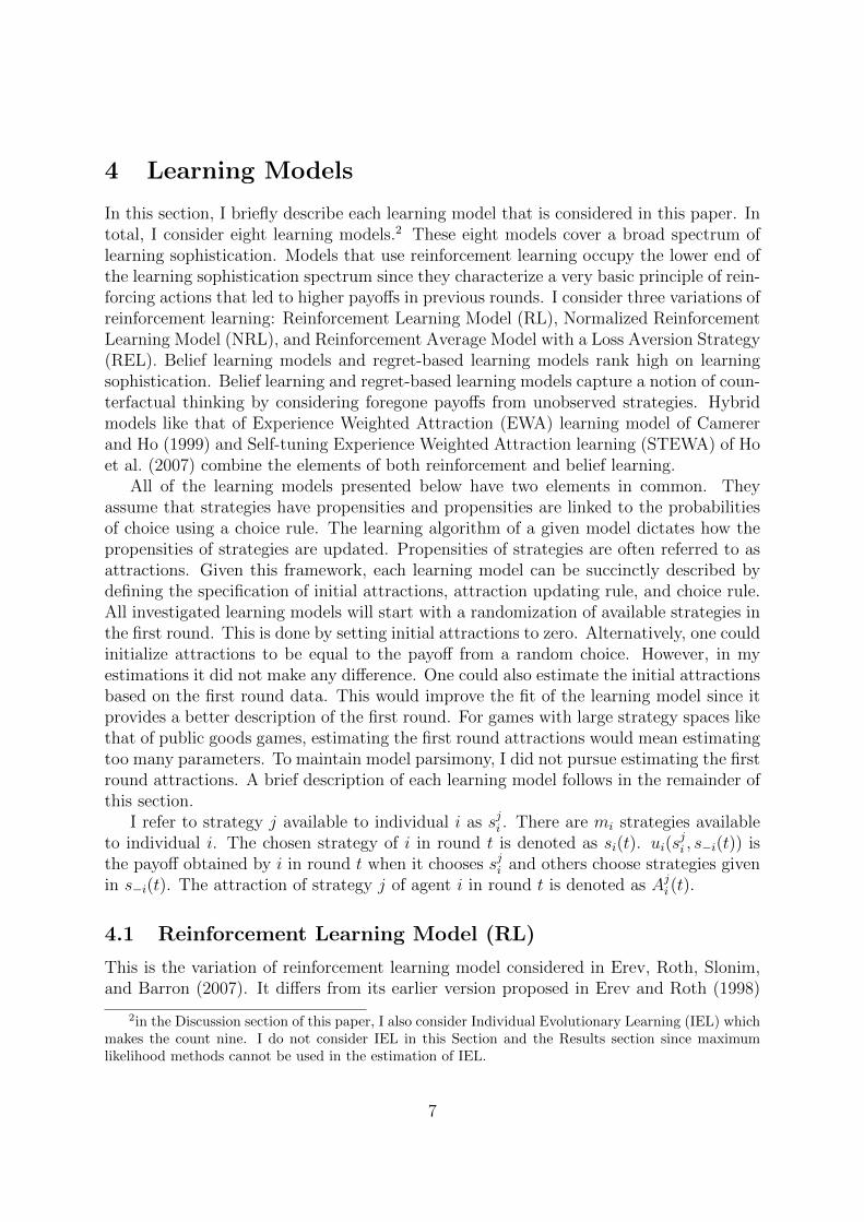
4 Learning Models
In this section, I briefly describe each learning model that is considered in this paper. Intotal, I consider eight learning models.2 These eight models cover a broad spectrum oflearning sophistication. Models that use reinforcement learning occupy the lower end ofthe learning sophistication spectrum since they characterize a very basic principle of rein-forcing actions that led to higher payoffs in previous rounds. I consider three variations ofreinforcement learning: Reinforcement Learning Model (RL), Normalized ReinforcementLearning Model (NRL), and Reinforcement Average Model with a Loss Aversion Strategy(REL). Belief learning models and regret-based learning models rank high on learningsophistication. Belief learning and regret-based learning models capture a notion of coun-terfactual thinking by considering foregone payoffs from unobserved strategies. Hybridmodels like that of Experience Weighted Attraction (EWA) learning model of Camererand Ho (1999) and Self-tuning Experience Weighted Attraction learning (STEWA) of Hoet al. (2007) combine the elements of both reinforcement and belief learning.
All of the learning models presented below have two elements in common. Theyassume that strategies have propensities and propensities are linked to the probabilitiesof choice using a choice rule. The learning algorithm of a given model dictates how thepropensities of strategies are updated. Propensities of strategies are often referred to asattractions. Given this framework, each learning model can be succinctly described bydefining the specification of initial attractions, attraction updating rule, and choice rule.All investigated learning models will start with a randomization of available strategies inthe first round. This is done by setting initial attractions to zero. Alternatively, one couldinitialize attractions to be equal to the payoff from a random choice. However, in myestimations it did not make any difference. One could also estimate the initial attractionsbased on the first round data. This would improve the fit of the learning model since itprovides a better description of the first round. For games with large strategy spaces likethat of public goods games, estimating the first round attractions would mean estimatingtoo many parameters. To maintain model parsimony, I did not pursue estimating the firstround attractions. A brief description of each learning model follows in the remainder ofthis section.
I refer to strategy j available to individual i as sji . There are mi strategies availableto individual i. The chosen strategy of i in round t is denoted as si(t). ui(s
ji , s−i(t)) is
the payoff obtained by i in round t when it chooses sji and others choose strategies givenin s−i(t). The attraction of strategy j of agent i in round t is denoted as Aji (t).
4.1 Reinforcement Learning Model (RL)
This is the variation of reinforcement learning model considered in Erev, Roth, Slonim,and Barron (2007). It differs from its earlier version proposed in Erev and Roth (1998)
2in the Discussion section of this paper, I also consider Individual Evolutionary Learning (IEL) whichmakes the count nine. I do not consider IEL in this Section and the Results section since maximumlikelihood methods cannot be used in the estimation of IEL.
7
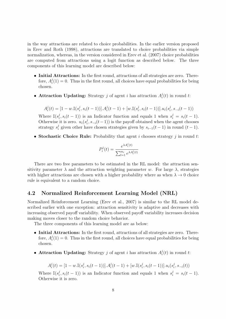
in the way attractions are related to choice probabilities. In the earlier version proposedin Erev and Roth (1998), attractions are translated to choice probabilities via simplenormalization, whereas, in the version considered in Erev et al. (2007) choice probabilitiesare computed from attractions using a logit function as described below. The threecomponents of this learning model are described below:
• Initial Attractions: In the first round, attractions of all strategies are zero. There-fore, Aji (1) = 0. Thus in the first round, all choices have equal probabilities for beingchosen.
• Attraction Updating: Strategy j of agent i has attraction Aji (t) in round t:
Aji (t) = [1− w.I(sji , si(t− 1))].Aji (t− 1) + [w.I(sji , si(t− 1))].ui(sji , s−i(t− 1))
Where I(sji , si(t − 1)) is an Indicator function and equals 1 when sji = si(t − 1).Otherwise it is zero. ui(s
ji , s−i(t−1)) is the payoff obtained when the agent chooses
strategy sji given other have chosen strategies given by si−1(t− 1) in round (t− 1).
• Stochastic Choice Rule: Probability that agent i chooses strategy j in round t:
P ji (t) =
eλAji (t)∑mi
l=1 eλAjl (t)
There are two free parameters to be estimated in the RL model: the attraction sen-sitivity parameter λ and the attraction weighting parameter w. For large λ, strategieswith higher attractions are chosen with a higher probability where as when λ→ 0 choicerule is equivalent to a random choice.
4.2 Normalized Reinforcement Learning Model (NRL)
Normalized Reinforcement Learning (Erev et al., 2007) is similar to the RL model de-scribed earlier with one exception: attraction sensitivity is adaptive and decreases withincreasing observed payoff variability. When observed payoff variability increases decisionmaking moves closer to the random choice behavior.
The three components of this learning model are as below:
• Initial Attractions: In the first round, attractions of all strategies are zero. There-fore, Aji (1) = 0. Thus in the first round, all choices have equal probabilities for beingchosen.
• Attraction Updating: Strategy j of agent i has attraction Aji (t) in round t:
Aji (t) = [1− w.I(sji , si(t− 1))].Aji (t− 1) + [w.I(sji , si(t− 1))].ui(sji , s−i(t))
Where I(sji , si(t − 1)) is an Indicator function and equals 1 when sji = si(t − 1).Otherwise it is zero.
8
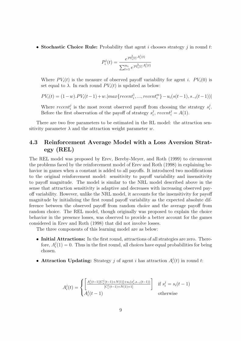
• Stochastic Choice Rule: Probability that agent i chooses strategy j in round t:
P ji (t) =
eλ
PVi(t)Aji (t)∑mi
l=1 eλ
PVi(t)Ajl (t)
Where PVi(t) is the measure of observed payoff variability for agent i. PVi(0) isset equal to λ. In each round PVi(t) is updated as below:
PVi(t) = (1−w).PVi(t−1)+w.|max{recent1i , ..., recentmi }−ui(s(t−1), s−i(t−1))|
Where recentji is the most recent observed payoff from choosing the strategy sji .Before the first observation of the payoff of strategy sji , recent
ji = A(1).
There are two free parameters to be estimated in the RL model: the attraction sen-sitivity parameter λ and the attraction weight parameter w.
4.3 Reinforcement Average Model with a Loss Aversion Strat-egy (REL)
The REL model was proposed by Erev, Bereby-Meyer, and Roth (1999) to circumventthe problems faced by the reinforcement model of Erev and Roth (1998) in explaining be-havior in games when a constant is added to all payoffs. It introduced two modificationsto the original reinforcement model: sensitivity to payoff variability and insensitivityto payoff magnitude. The model is similar to the NRL model described above in thesense that attraction sensitivity is adaptive and decreases with increasing observed pay-off variability. However, unlike the NRL model, it accounts for the insensitivity for payoffmagnitude by initializing the first round payoff variability as the expected absolute dif-ference between the observed payoff from random choice and the average payoff fromrandom choice. The REL model, though originally was proposed to explain the choicebehavior in the presence losses, was observed to provide a better account for the gamesconsidered in Erev and Roth (1998) that did not involve losses.
The three components of this learning model are as below:
• Initial Attractions: In the first round, attractions of all strategies are zero. There-fore, Aji (1) = 0. Thus in the first round, all choices have equal probabilities for beingchosen.
• Attraction Updating: Strategy j of agent i has attraction Aji (t) in round t:
Aji (t) =
[Aji (t−1)[C
ji (t−1)+N(1)]+ui(s
ji ,s−i(t−1))
[Cji (t−1)+N(1)+1]
]if sji = si(t− 1)
Aji (t− 1) otherwise
9

where Cji (t) is the number of times sji has been chosen in the first t rounds and
N(1) is a free parameter that determines the strength of the initial attractions. Alarge N(1) means that effect of actual payoffs in later rounds on attractions will besmaller. The attractions of unchosen strategies are not updated.
• Stochastic Choice Rule: Probability that agent i chooses strategy j in round t:
P ji (t) =
eλ
PVi(t)Aji (t)∑mi
l=1 eλ
PVi(t)Ajl (t)
where λi is a free parameter that determines the reinforcement sensitivity of theindividual i. PVi(t) is the measure of payoff variability.
The payoff variability is updated according to:
PVi(t) =[PVi(t− 1)(t− 1 +miN(1)) + |ui(si(t− 1), s−i(t− 1))− PAi(t− 1)|]
[t+miN(1)]
where PAi(t) is the accumulated payoff average in round t and m is the number ofstrategies. PVi(1) > 0 is initialized as the the expected absolute difference betweenthe obtained payoff from a random choice and the average payoff from a randomchoice.
PAi(t) is calculated in a similar manner.
PAi(t) =[PAi(t− 1)(t− 1 +miNi(1)) + ui(si(t− 1), s−i(t− 1))]
[t+miNi(1)]
I initialized PAi(1) as initial attraction of a any strategy which is 0. There aretwo free parameters to be estimated in the REL model: the attraction sensitivityparameter λ and the strength of initial attractions N(1).
4.4 Stochastic Fictitious Play (SFP)
Stochastic Fictitious Play (SFP) (Fudenberg & Levine, 1998; Cheung & Friedman, 1997;Cooper, Garvin, & Kagel, 1997) is a prototypical characterization of belief learning. HereI consider the variation of the model described in Erev et al. (2007).
• Initial Attractions: In the first round, attractions of all strategies are zero. There-fore, Aji (1) = 0. Thus in the first round, all choices have equal probabilities for beingchosen.
• Attraction Updating: Strategy j of agent i has attraction Aji (t) in round t:
Aji (t) = [1− w].Aji (t− 1) + w.ui(sji , s−i(t− 1))
ui(sji , s−i(t − 1)) is the payoff obtained when the agent chooses strategy sji given
other have chosen strategies given by s−i(t− 1) in round (t− 1).
10
• Stochastic Choice Rule: Probability that agent i chooses strategy j in round t:
P ji (t) =
eλAji (t)∑mi
l=1 eλAjl (t)
There are two free parameters to be estimated in the SFP model: the attractionsensitivity parameter λ and the attraction weight parameter w.
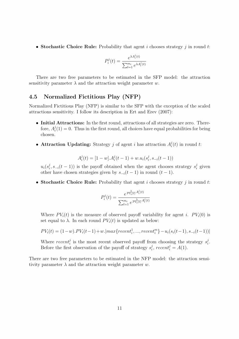
4.5 Normalized Fictitious Play (NFP)
Normalized Fictitious Play (NFP) is similar to the SFP with the exception of the scaledattractions sensitivity. I follow its description in Ert and Erev (2007):
• Initial Attractions: In the first round, attractions of all strategies are zero. There-fore, Aji (1) = 0. Thus in the first round, all choices have equal probabilities for beingchosen.
• Attraction Updating: Strategy j of agent i has attraction Aji (t) in round t:
Aji (t) = [1− w].Aji (t− 1) + w.ui(sji , s−i(t− 1))
ui(sji , s−i(t − 1)) is the payoff obtained when the agent chooses strategy sji given
other have chosen strategies given by s−i(t− 1) in round (t− 1).
• Stochastic Choice Rule: Probability that agent i chooses strategy j in round t:
P ji (t) =
eλ
PVi(t)Aji (t)∑mi
l=1 eλ
PVi(t)Ajl (t)
Where PVi(t) is the measure of observed payoff variability for agent i. PVi(0) isset equal to λ. In each round PVi(t) is updated as below:
PVi(t) = (1−w).PVi(t−1)+w.|max{recent1i , ..., recentmi }−ui(si(t−1), s−i(t−1))|
Where recentji is the most recent observed payoff from choosing the strategy sji .Before the first observation of the payoff of strategy sji , recent
ji = A(1).
There are two free parameters to be estimated in the NFP model: the attraction sensi-tivity parameter λ and the attraction weight parameter w.
11
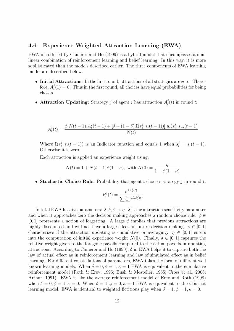
4.6 Experience Weighted Attraction Learning (EWA)
EWA introduced by Camerer and Ho (1999) is a hybrid model that encompasses a non-linear combination of reinforcement learning and belief learning. In this way, it is moresophisticated than the models described earlier. The three components of EWA learningmodel are described below.
• Initial Attractions: In the first round, attractions of all strategies are zero. There-fore, Aji (1) = 0. Thus in the first round, all choices have equal probabilities for beingchosen.
• Attraction Updating: Strategy j of agent i has attraction Aji (t) in round t:
Aji (t) =φ.N(t− 1).Aji (t− 1) + [δ + (1− δ).I(sji , si(t− 1))].ui(s
ji , s−i(t− 1)
N(t)
Where I(sji , si(t − 1)) is an Indicator function and equals 1 when sji = si(t − 1).Otherwise it is zero.
Each attraction is applied an experience weight using:
N(t) = 1 +N(t− 1)φ(1− κ), with N(0) =η
1− φ(1− κ)
• Stochastic Choice Rule: Probability that agent i chooses strategy j in round t:
P ji (t) =
eλAji (t)∑mi
l=1 eλAjl (t)
In total EWA has five parameters: λ, δ, φ, κ, η. λ is the attraction sensitivity parameterand when it approaches zero the decision making approaches a random choice rule. φ ∈[0, 1] represents a notion of forgetting. A large φ implies that previous attractions arehighly discounted and will not have a large effect on future decision making. κ ∈ [0, 1]characterizes if the attraction updating is cumulative or averaging. η ∈ [0, 1] entersinto the computation of initial experience weight N(0). Finally, δ ∈ [0, 1] captures therelative weight given to the foregone payoffs compared to the actual payoffs in updatingattractions. According to Camerer and Ho (1999), δ in EWA helps it to capture both thelaw of actual effect as in reinforcement learning and law of simulated effect as in belieflearning. For different constellations of parameters, EWA takes the form of different wellknown learning models. When δ = 0, φ = 1, κ = 1 EWA is equivalent to the cumulativereinforcement model (Roth & Erev, 1995; Bush & Mosteller, 1955; Cross et al., 2008;Arthur, 1991). EWA is like the average reinforcement model of Erev and Roth (1998)when δ = 0, φ = 1, κ = 0. When δ = 1, φ = 0, κ = 1 EWA is equivalent to the Cournotlearning model. EWA is identical to weighted fictitious play when δ = 1, φ = 1, κ = 0.
12
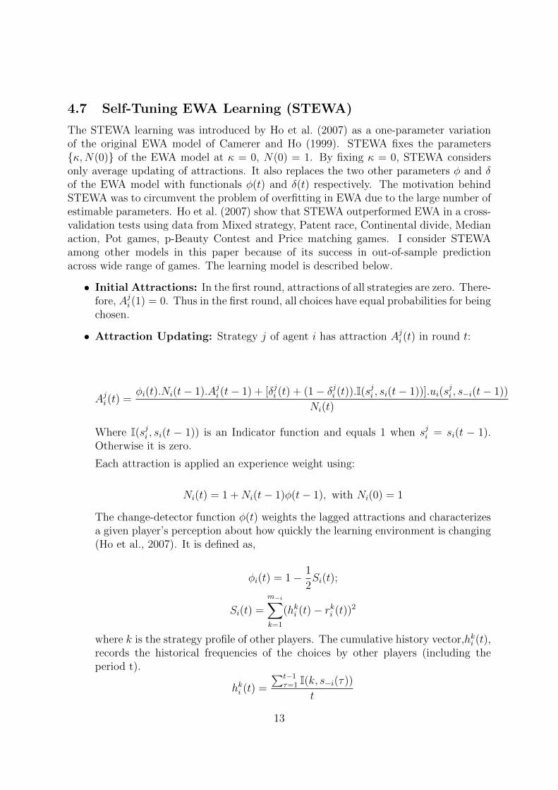
4.7 Self-Tuning EWA Learning (STEWA)
The STEWA learning was introduced by Ho et al. (2007) as a one-parameter variationof the original EWA model of Camerer and Ho (1999). STEWA fixes the parameters{κ,N(0)} of the EWA model at κ = 0, N(0) = 1. By fixing κ = 0, STEWA considersonly average updating of attractions. It also replaces the two other parameters φ and δof the EWA model with functionals φ(t) and δ(t) respectively. The motivation behindSTEWA was to circumvent the problem of overfitting in EWA due to the large number ofestimable parameters. Ho et al. (2007) show that STEWA outperformed EWA in a cross-validation tests using data from Mixed strategy, Patent race, Continental divide, Medianaction, Pot games, p-Beauty Contest and Price matching games. I consider STEWAamong other models in this paper because of its success in out-of-sample predictionacross wide range of games. The learning model is described below.
• Initial Attractions: In the first round, attractions of all strategies are zero. There-fore, Aji (1) = 0. Thus in the first round, all choices have equal probabilities for beingchosen.
• Attraction Updating: Strategy j of agent i has attraction Aji (t) in round t:
Aji (t) =φi(t).Ni(t− 1).Aji (t− 1) + [δji (t) + (1− δji (t)).I(s
ji , si(t− 1))].ui(s
ji , s−i(t− 1))
Ni(t)
Where I(sji , si(t − 1)) is an Indicator function and equals 1 when sji = si(t − 1).Otherwise it is zero.
Each attraction is applied an experience weight using:
Ni(t) = 1 +Ni(t− 1)φ(t− 1), with Ni(0) = 1
The change-detector function φ(t) weights the lagged attractions and characterizesa given player’s perception about how quickly the learning environment is changing(Ho et al., 2007). It is defined as,
φi(t) = 1− 1
2Si(t);
Si(t) =
m−i∑k=1
(hki (t)− rki (t))2
where k is the strategy profile of other players. The cumulative history vector,hki (t),records the historical frequencies of the choices by other players (including theperiod t).
hki (t) =
∑t−1τ=1 I(k, s−i(τ))
t
13
where s−i(τ) is the observed choice of strategies by others in round τ . The im-mediate history vector, rki (t), is a vector of 1’s and 0’s. Therefore in the round t,rki (t) = I(k, s−i(t). S(t) is the quadratic distance between the cumulative historyvector hki (t) and the immediate history vector rki (t). It captures the degree of sur-prise due to change in the observed choices of the other players. It will always liebetween 0 and 2 and so φi(t) lies in between 0 and 1.
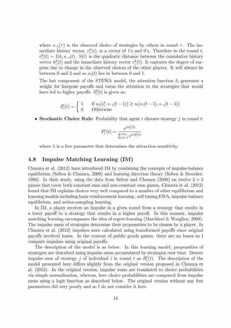
The last component of the STEWA model, the attention function δi generates aweight for foregone payoffs and turns the attention to the strategies that wouldhave led to higher payoffs. δqi (t) is given as:
δqi (t) =
{1 if ui(s
qi , s−i(t− 1)) ≥ ui(si(t− 1), s−i(t− 1))
0 Otherwise
• Stochastic Choice Rule: Probability that agent i chooses strategy j in round t:
P ji (t) =
eλAji (t)∑mi
l=1 eλAjl (t)
where λ is a free parameter that determines the attraction sensitivity.
4.8 Impulse Matching Learning (IM)
Chmura et al. (2012) have introduced IM by combining the concepts of impulse-balanceequilibrium (Selten & Chmura, 2008) and learning direction theory (Selten & Stoecker,1986). In their study, using the data from Selten and Chmura (2008) on twelve 2 × 2games that cover both constant sum and non-constant sum games, Chmura et al. (2012)found that IM explains choices very well compared to a number of other equilibrium andlearning models including basic reinforcement learning , self tuning EWA, impulse-balanceequilibrium, and action-sampling learning.
In IM, a player receives an impulse in a given round from a strategy that results ina lower payoff to a strategy that results in a higher payoff. In this manner, impulsematching learning encompasses the idea of regret-learning (Marchiori & Warglien, 2008).The impulse sums of strategies determine their propensities to be chosen by a player. InChmura et al. (2012) impulses were calculated using transformed payoffs since originalpayoffs involved losses. In the context of public goods games, there are no losses so Icompute impulses using original payoffs.
The description of the model is as below. In this learning model, propensities ofstrategies are described using impulse sums accumulated by strategies over time. Denoteimpulse sum of strategy j of individual i in round t as Rj
i (t). The description of themodel presented here differs slightly from the original version proposed in Chmura etal. (2012). In the original version, impulse sums are translated to choice probabilitiesvia simple normalization, whereas, here choice probabilities are computed from impulsesums using a logit function as described below. The original version without any freeparameters did very poorly and so I do not consider it here.
14
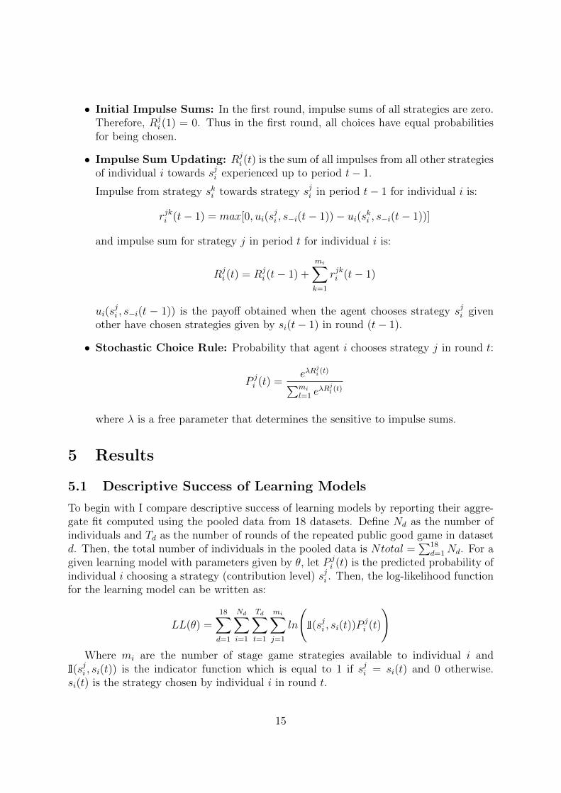
• Initial Impulse Sums: In the first round, impulse sums of all strategies are zero.Therefore, Rj
i (1) = 0. Thus in the first round, all choices have equal probabilitiesfor being chosen.
• Impulse Sum Updating: Rji (t) is the sum of all impulses from all other strategies
of individual i towards sji experienced up to period t− 1.
Impulse from strategy ski towards strategy sji in period t− 1 for individual i is:
rjki (t− 1) = max[0, ui(sji , s−i(t− 1))− ui(ski , s−i(t− 1))]
and impulse sum for strategy j in period t for individual i is:
Rji (t) = Rj
i (t− 1) +
mi∑k=1
rjki (t− 1)
ui(sji , s−i(t − 1)) is the payoff obtained when the agent chooses strategy sji given
other have chosen strategies given by si(t− 1) in round (t− 1).
• Stochastic Choice Rule: Probability that agent i chooses strategy j in round t:
P ji (t) =
eλRji (t)∑mi
l=1 eλRjl (t)
where λ is a free parameter that determines the sensitive to impulse sums.
5 Results
5.1 Descriptive Success of Learning Models
To begin with I compare descriptive success of learning models by reporting their aggre-gate fit computed using the pooled data from 18 datasets. Define Nd as the number ofindividuals and Td as the number of rounds of the repeated public good game in datasetd. Then, the total number of individuals in the pooled data is Ntotal =
∑18d=1Nd. For a
given learning model with parameters given by θ, let P ji (t) is the predicted probability of
individual i choosing a strategy (contribution level) sji . Then, the log-likelihood functionfor the learning model can be written as:
LL(θ) =18∑d=1
Nd∑i=1
Td∑t=1
mi∑j=1
ln
(I(sji , si(t))P
ji (t)
)Where mi are the number of stage game strategies available to individual i and
I(sji , si(t)) is the indicator function which is equal to 1 if sji = si(t) and 0 otherwise.si(t) is the strategy chosen by individual i in round t.
15
I used Broyden-Fletcher-Goldfarb-Shanno (BFGS) algorithm with numerical deriva-tives to maximize the log-likelihood function and estimate the parameters for each learn-ing model. The fit of each learning model is described using four metrics: Log-Likelihood(LL), Akaike Information Criterion (AIC), Bayesian Information Criterion (BIC), andPseudo-R2. LL is the maximum log-likelihood achieved by a learning model. The lastthree metrics are defined as below for a learning model:
AIC = LL− k
BIC = LL− k
2ln(Ntotal)
Pseudo-R2 =AIC − LLR
LLR
Where k is the number of parameters of the learning model, Ntotal is the total numberof observations, and LLR is the log-likelihood obtained by a random choice model. Sincechoices of an individual are not independent I consider the number of individuals as theeffective size of the sample in the computation of BIC. Therefore, Ntotal is equal to1201 here. AIC and BIC penalize models for their complexity and therefore are superiormetrics than log-likelihood for model comparison.
In evaluating models in terms of their descriptive and predictive success, I also considertwo basic benchmarks. The first benchmark is derived from a random choice model.Denote the random choice model as RAND. Since the datasets differ in terms of thenumber of strategies(contribution levels) available to individuals, it should be noted thatRAND model can only be derived at the dataset level. For example, in a dataset wherethe endowment is 20, e.g. as in DS9, RAND model predicts any given observed choice inthat data set with a probability of 1
21. Instead, if the endowment in a data set is 50 as in
DS1, RAND model predicts any given observed choice in that data set with a probabilityof 1
51. Obviously, the RAND benchmark is not a serious benchmark and I expect that
every learning model should beat it. The second benchmark is derived from a model thatis derived from the overall empirical frequencies of choices in each dataset. This modelis referred to as EMP in the remainder of the paper. In the context of my analysis,EMP has 18 degrees of freedom since it is derived separately for each dataset. Thus,it is allowed to differ across datasets. A problem in deriving one model for the pooleddata of 18 datasets is that, the number of strategies available to individuals varies acrossdatasets. Without some kind of artificial aggregation of strategies (for example, one canput available strategies into three groups as low contribution, medium contribution, highcontribution and then derive empirical frequencies of these constructed strategies acrossthe pooled data), one cannot derive a single model of empirical frequencies by combiningthe data from all datasets. Since EMP is based on observed empirical frequencies ofchoices and is derived at the dataset level, it has a strong potential to fit the data verywell. Thus, EMP is a very challenging benchmark for learning models to beat.If a learningtheory successfully describes choice adjustments over time in a data set, it would obtainbetter fit than EMP since the latter does not depend upon temporal information.
16
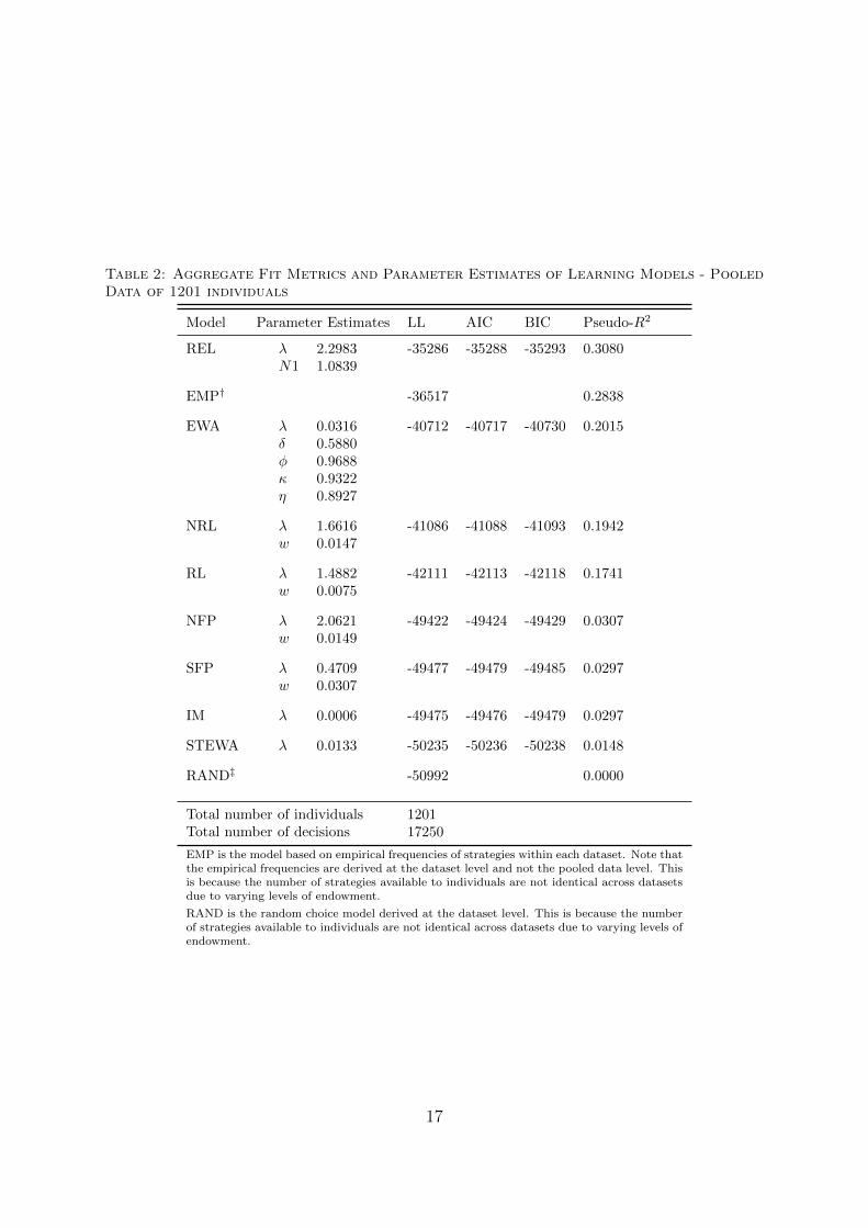
Table 2: Aggregate Fit Metrics and Parameter Estimates of Learning Models - PooledData of 1201 individuals
Model Parameter Estimates LL AIC BIC Pseudo-R2
REL λ 2.2983 -35286 -35288 -35293 0.3080N1 1.0839
EMP† -36517 0.2838
EWA λ 0.0316 -40712 -40717 -40730 0.2015δ 0.5880φ 0.9688κ 0.9322η 0.8927
NRL λ 1.6616 -41086 -41088 -41093 0.1942w 0.0147
RL λ 1.4882 -42111 -42113 -42118 0.1741w 0.0075
NFP λ 2.0621 -49422 -49424 -49429 0.0307w 0.0149
SFP λ 0.4709 -49477 -49479 -49485 0.0297w 0.0307
IM λ 0.0006 -49475 -49476 -49479 0.0297
STEWA λ 0.0133 -50235 -50236 -50238 0.0148
RAND‡ -50992 0.0000
Total number of individuals 1201Total number of decisions 17250
EMP is the model based on empirical frequencies of strategies within each dataset. Note thatthe empirical frequencies are derived at the dataset level and not the pooled data level. Thisis because the number of strategies available to individuals are not identical across datasetsdue to varying levels of endowment.
RAND is the random choice model derived at the dataset level. This is because the numberof strategies available to individuals are not identical across datasets due to varying levels ofendowment.
17
Table 2 presents the parameter estimates that maximized the log-likelihood of thepooled data for each learning model. It also presents four aggregate fit metrics com-puted using the maximum likelihood parameter estimates. The fit achieved by the twobenchmarks, RAND and EMP, is also reported for comparison. Using these results, thelearning models can be ordered in terms of their performance as REL, EWA, NRL, RL,SFP, NSFP, IM, STEWA. This ordering holds according to any of the four fit metricsthat are reported. REL outperforms all other models and the performance gap betweenREL and the second best performer EWA is quite large. This convinces at least from anaggregate descriptive fit point of view that REL explain the aggregate data convincinglybetter than all other models that are considered in this paper. As expected, all learningmodels are able to the perform better than the random choice benchmark. However,except REL all learning models fail to explain the data at least as well as EMP accordingto all four reported metrics. REL outperforms EMP meaning that REL is able to explainchoice adjustment over time.
One of the clear patterns in Table 2 is that reinforcement learning models do relativelybetter in comparison to belief learning or regret learning models in explaining the data.Furthermore, models with adaptive attraction sensitivity, i.e. NRL and NFP, fit bettercompared to their counterparts, i. e. RL and SFP. Thus, adaptive attraction sensitivitythat depends upon observed payoff variability seems to be important in explaining be-havior in repeated public goods games. Despite having more degrees of freedom, EWAperforms significantly worse than REL. IM and STEWA lie at the bottom of the tableand perform marginally (but significantly according to likelihood ratio tests) better thana random choice model.
Another way to look into descriptive success of a learning model is by evaluatinghow well one set of parameters of the model that is estimated using the pooled data canexplain observed choices in different datasets that correspond to different sets of gameparameters. This is one way to evaluate the generalizability of a given learning model interms of its descriptive success. A model that is generalizable should be able to explainbehavior across games with varying game parameters (MPCR, endowment, number ofrounds, and matching) without the need to adjust its learning parameters based on theparameters of the games. To evaluate models’ descriptive generalizability, I computeLL, BIC, and Mean Quadratic Score of each learning model for each of the 18 datasetsseparately. In doing so, I use the parameter estimates of each learning model computedfrom the pooled data reported in Table 2.
The computation of LL and BIC was introduced earlier. Mean Quadratic Score (MQS)of a learning model is computed for a dataset using the quadratic scoring rule. Thequadratic scoring rule was first introduced by Brier (1950), and was axiomatically char-acterized in Selten (1998). Let, for a subject i in round t of a repeated game, a givenlearning model predicts each strategy sij with a probability pij(t). If the subject’s observedstrategy in round t is sik, then the quadratic score of the learning model in round t isgiven as:
18
qi(t) = 2pik(t)−mi∑j=1
(pij(t))2
Thus, in computing the quadratic score, the observed choice is interpreted as a de-generate probability distribution with observed strategy having a probability of 1 and allother strategies having a probability of 0. The quadratic score ranges between [-1, +1].3
Higher scores indicate the relative success of a model in predicting observed choices.If there are Nd individuals in dataset d and the public goods game is repeated for Td
rounds, then the MQS achieved by the learning model for the dataset d is:
MQS =
Nd∑i=1
[ Td∑t=1
qi(t)
Nd × Td
]Table 3 compares LL, BIC, and MQS achieved by each learning model at the dataset
level. For each learning model, I compute the three fit metrics for each of the 18 datasets.For each pair of learning models, one sided p-value favoring the learning model in the rowis reported using the 18 measures of each fit metric computed at the dataset level. Thep-values are computed using the Exact Wilcoxon Signed-Rank Test for matched pairs.The results in Table 3 lead to similar conclusions as in Table 2. REL outperforms allother learning models in terms its descriptive success at the dataset level according to LL,BIC, and MQS metrics. This indicates that the parameter estimates of REL obtainedusing the estimation with pooled data are quite general that they explain behavior indifferent public goods games with parameters spanning a broad spectrum. What thisindicates is that the parameters of REL need not to be significantly adjusted basedon the parameters of the game to describe choice behavior in it. REL outperformsEMP in terms of MQS but performs equally as well as EMP in terms of LL and BIC.However, one need to keep in mind that EMP is a very tough benchmark to beat sincethe EMP model is derived separately for each data set helping it to fine tune its fitat the data set level. None of the other learning models are able to outperform EMPaccording to LL and BIC. NRL, EWA, and RL perform as well as EMP in terms ofMQS. NRL and EWA jointly take the second place. They both perform equally well inexplaining behavior across datasets with one set of parameters according to LL, BIC,and MQS metrics. RL comes third. As observed earlier, belief learning models do notperform well in explaining the data in comparison to the reinforcement models. NSFP,SFP, IM, and STEWA are statistically indistinguishable in terms of their performance.It is interesting to note that the top two models, REL and NRL, are similar in thesense they both use adapt attraction sensitivity based on the observed payoff variability.NRL performs significantly better than RL which is its identical counterpart without
3If the observed choice is completely in line with prediction of the model then quadratic score achieves+1. This happens if the model puts a probability of one on the observed choice. The quadratic scorewould be minimum at -1 if the model puts all the probability on a strategy different from that of theobserved strategy. All other probability distributions over strategies result in a score strictly between -1and +1.
19
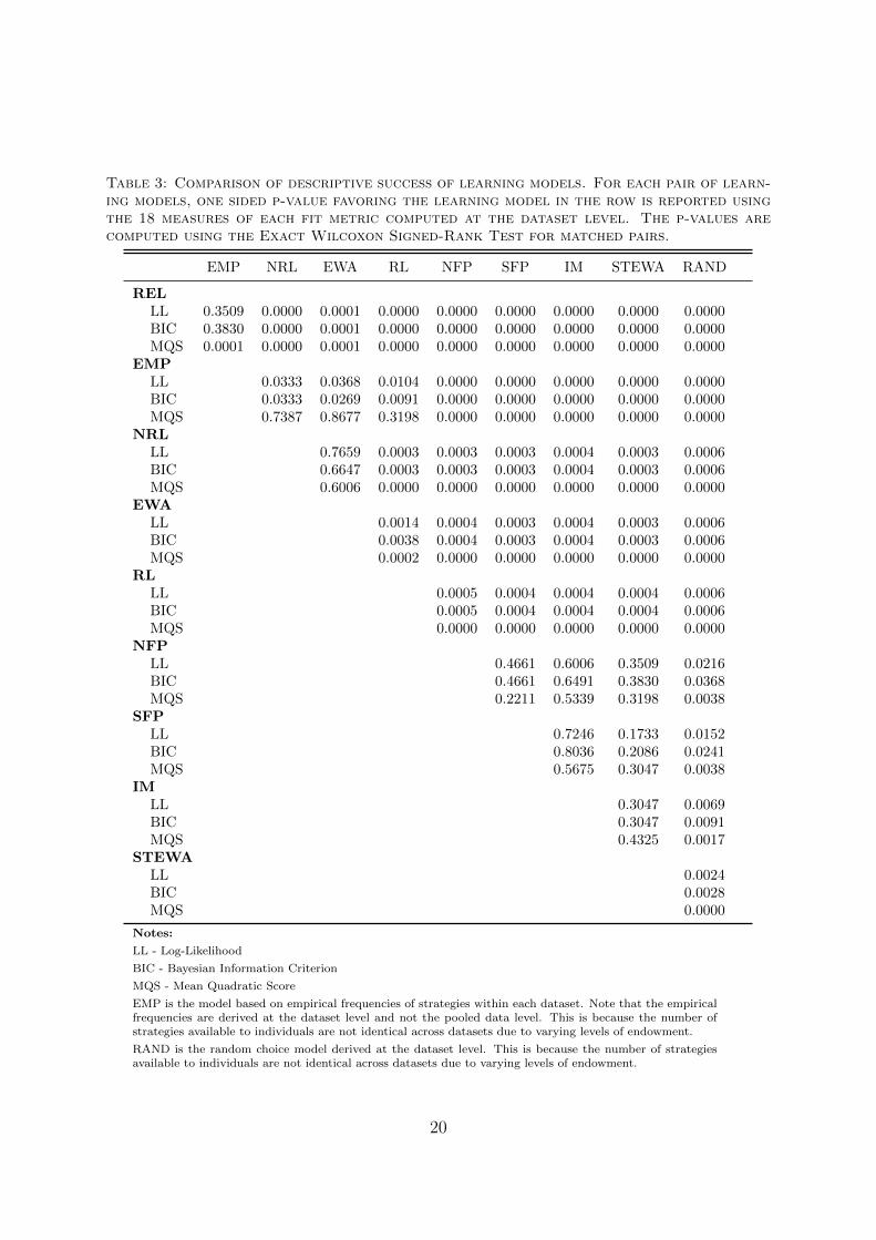
Table 3: Comparison of descriptive success of learning models. For each pair of learn-ing models, one sided p-value favoring the learning model in the row is reported usingthe 18 measures of each fit metric computed at the dataset level. The p-values arecomputed using the Exact Wilcoxon Signed-Rank Test for matched pairs.
EMP NRL EWA RL NFP SFP IM STEWA RAND
RELLL 0.3509 0.0000 0.0001 0.0000 0.0000 0.0000 0.0000 0.0000 0.0000BIC 0.3830 0.0000 0.0001 0.0000 0.0000 0.0000 0.0000 0.0000 0.0000MQS 0.0001 0.0000 0.0001 0.0000 0.0000 0.0000 0.0000 0.0000 0.0000
EMPLL 0.0333 0.0368 0.0104 0.0000 0.0000 0.0000 0.0000 0.0000BIC 0.0333 0.0269 0.0091 0.0000 0.0000 0.0000 0.0000 0.0000MQS 0.7387 0.8677 0.3198 0.0000 0.0000 0.0000 0.0000 0.0000
NRLLL 0.7659 0.0003 0.0003 0.0003 0.0004 0.0003 0.0006BIC 0.6647 0.0003 0.0003 0.0003 0.0004 0.0003 0.0006MQS 0.6006 0.0000 0.0000 0.0000 0.0000 0.0000 0.0000
EWALL 0.0014 0.0004 0.0003 0.0004 0.0003 0.0006BIC 0.0038 0.0004 0.0003 0.0004 0.0003 0.0006MQS 0.0002 0.0000 0.0000 0.0000 0.0000 0.0000
RLLL 0.0005 0.0004 0.0004 0.0004 0.0006BIC 0.0005 0.0004 0.0004 0.0004 0.0006MQS 0.0000 0.0000 0.0000 0.0000 0.0000
NFPLL 0.4661 0.6006 0.3509 0.0216BIC 0.4661 0.6491 0.3830 0.0368MQS 0.2211 0.5339 0.3198 0.0038
SFPLL 0.7246 0.1733 0.0152BIC 0.8036 0.2086 0.0241MQS 0.5675 0.3047 0.0038
IMLL 0.3047 0.0069BIC 0.3047 0.0091MQS 0.4325 0.0017
STEWALL 0.0024BIC 0.0028MQS 0.0000
Notes:
LL - Log-Likelihood
BIC - Bayesian Information Criterion
MQS - Mean Quadratic Score
EMP is the model based on empirical frequencies of strategies within each dataset. Note that the empiricalfrequencies are derived at the dataset level and not the pooled data level. This is because the number ofstrategies available to individuals are not identical across datasets due to varying levels of endowment.
RAND is the random choice model derived at the dataset level. This is because the number of strategiesavailable to individuals are not identical across datasets due to varying levels of endowment.
20
the dynamic attraction sensitivity adjustment confirming adaptive attraction sensitivityis an important construct in explaining behavior in repeated public goods games. Inaddition, REL scales the initial attraction sensitivity parameter using the expected payoffvariability due to a random choice. What this scaling does is, it makes the learning modelinsensitive to payoff magnitudes. This appears to be instrumental in explaining learningbehavior across different datasets involving a wide range possible payoffs. Thus, bothof these features, the dynamic adjustment of attraction sensitivity based on observedpayoff variability and the scaling of initial attraction sensitivity using a baseline payoffvariability, appear to be important components of a learning model that does successfullyexplain behavior in repeated public goods games across a wide range of game parameters.
5.2 Predictive Accuracy of Learning Models
A more challenging test of model robustness and generalizability concerns with out-of-sample predictive accuracy of a given model. This line of analysis was pioneered in thecontext of learning in games in earlier studies by Erev and Roth (1998) and Ho et al.(2007). These studies have compared learning models by first estimating the parametersof the models using data on a set of games and then comparing how well the modelspredict choices in a new game with the estimated model parameters. My analysis here isdifferent in that I study only one type of games here. But, the parameters of the game varyacross datasets. To compare the out-of-sample predictive accuracy of learning models,I predict choices according to each learning model in each of the 18 datasets using theparameters estimated for the learning model using the remaining 17 datasets excludingthe data set under consideration. These results test whether a model that is fitted usingthe data on public goods games with a set of given parameters (e.g. group size, marginalper capita return, number of rounds, matching protocol) can successfully predict choicesin a public goods game with a set of game parameters that was not observed previously.
I characterize dataset level predictive accuracy of each learning model using five met-rics: LL, AIC, BIC, Pseudo-R2, and Mean Quadratic Score (MQS). Table 4 presentsresults about the predictive accuracy of models. For each dataset, I report LL, AIC,BIC, Pseudo-R2, MQS achieved by each learning model with the parameters estimatedfrom the remaining 17 datasets. The performance of RAND and EMP benchmarks isalso reported for each dataset. Both of these benchmarks represent models derived atthe data set level using the data within the dataset. In that sense, their scores do notreflect their predictive success but their descriptive success. A challenge in reporting pre-dictive accuracy of these models is that data from different datasets cannot be pooled toderive empirical frequencies since the datasets vary in terms of the number of strategies(meaning they involve different levels of endowment) available to individuals. Since EMPreflects within data set empirical frequencies, it is impressive for a learning model if itcan do as well as or better than EMP in prediction. In Table 4 , I marked the best scoreachieved for a given data set by any learning model with an asterisk. I marked EMPwith a dagger in data sets where none of the learning models performed at least well asEMP in their predictions.
21
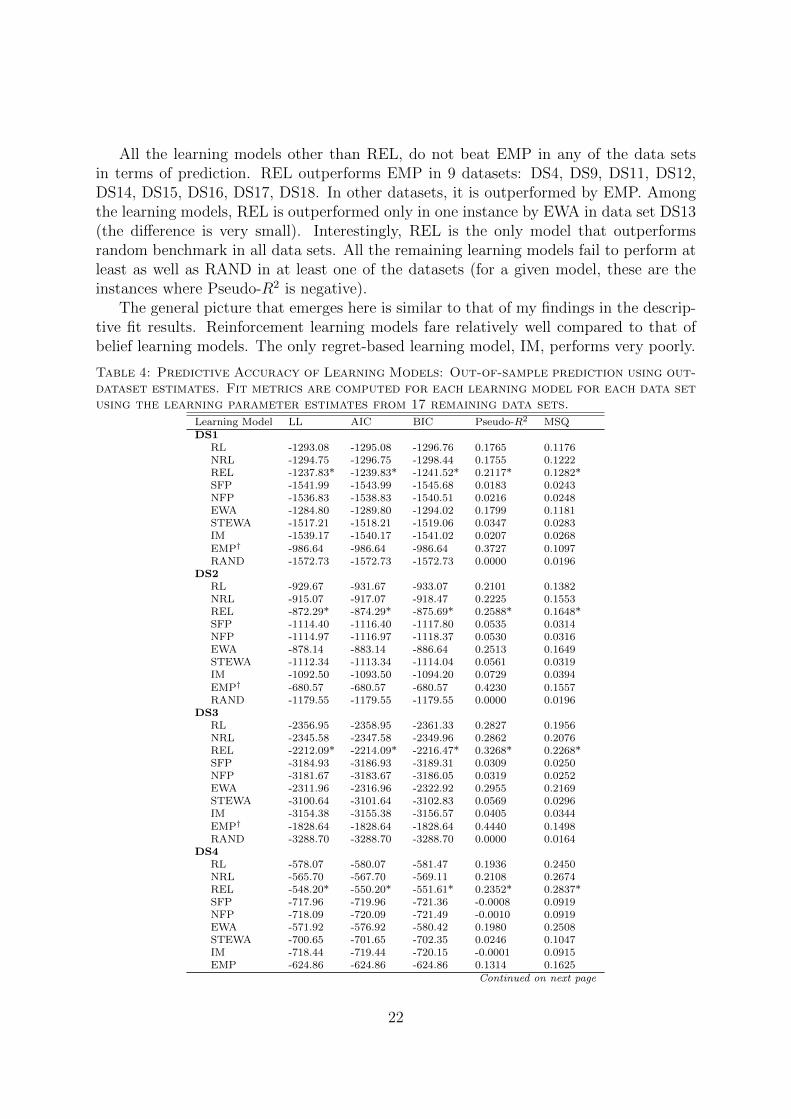
All the learning models other than REL, do not beat EMP in any of the data setsin terms of prediction. REL outperforms EMP in 9 datasets: DS4, DS9, DS11, DS12,DS14, DS15, DS16, DS17, DS18. In other datasets, it is outperformed by EMP. Amongthe learning models, REL is outperformed only in one instance by EWA in data set DS13(the difference is very small). Interestingly, REL is the only model that outperformsrandom benchmark in all data sets. All the remaining learning models fail to perform atleast as well as RAND in at least one of the datasets (for a given model, these are theinstances where Pseudo-R2 is negative).
The general picture that emerges here is similar to that of my findings in the descrip-tive fit results. Reinforcement learning models fare relatively well compared to that ofbelief learning models. The only regret-based learning model, IM, performs very poorly.
Table 4: Predictive Accuracy of Learning Models: Out-of-sample prediction using out-dataset estimates. Fit metrics are computed for each learning model for each data setusing the learning parameter estimates from 17 remaining data sets.
Learning Model LL AIC BIC Pseudo-R2 MSQDS1
RL -1293.08 -1295.08 -1296.76 0.1765 0.1176NRL -1294.75 -1296.75 -1298.44 0.1755 0.1222REL -1237.83* -1239.83* -1241.52* 0.2117* 0.1282*SFP -1541.99 -1543.99 -1545.68 0.0183 0.0243NFP -1536.83 -1538.83 -1540.51 0.0216 0.0248EWA -1284.80 -1289.80 -1294.02 0.1799 0.1181STEWA -1517.21 -1518.21 -1519.06 0.0347 0.0283IM -1539.17 -1540.17 -1541.02 0.0207 0.0268EMP† -986.64 -986.64 -986.64 0.3727 0.1097RAND -1572.73 -1572.73 -1572.73 0.0000 0.0196
DS2RL -929.67 -931.67 -933.07 0.2101 0.1382NRL -915.07 -917.07 -918.47 0.2225 0.1553REL -872.29* -874.29* -875.69* 0.2588* 0.1648*SFP -1114.40 -1116.40 -1117.80 0.0535 0.0314NFP -1114.97 -1116.97 -1118.37 0.0530 0.0316EWA -878.14 -883.14 -886.64 0.2513 0.1649STEWA -1112.34 -1113.34 -1114.04 0.0561 0.0319IM -1092.50 -1093.50 -1094.20 0.0729 0.0394EMP† -680.57 -680.57 -680.57 0.4230 0.1557RAND -1179.55 -1179.55 -1179.55 0.0000 0.0196
DS3RL -2356.95 -2358.95 -2361.33 0.2827 0.1956NRL -2345.58 -2347.58 -2349.96 0.2862 0.2076REL -2212.09* -2214.09* -2216.47* 0.3268* 0.2268*SFP -3184.93 -3186.93 -3189.31 0.0309 0.0250NFP -3181.67 -3183.67 -3186.05 0.0319 0.0252EWA -2311.96 -2316.96 -2322.92 0.2955 0.2169STEWA -3100.64 -3101.64 -3102.83 0.0569 0.0296IM -3154.38 -3155.38 -3156.57 0.0405 0.0344EMP† -1828.64 -1828.64 -1828.64 0.4440 0.1498RAND -3288.70 -3288.70 -3288.70 0.0000 0.0164
DS4RL -578.07 -580.07 -581.47 0.1936 0.2450NRL -565.70 -567.70 -569.11 0.2108 0.2674REL -548.20* -550.20* -551.61* 0.2352* 0.2837*SFP -717.96 -719.96 -721.36 -0.0008 0.0919NFP -718.09 -720.09 -721.49 -0.0010 0.0919EWA -571.92 -576.92 -580.42 0.1980 0.2508STEWA -700.65 -701.65 -702.35 0.0246 0.1047IM -718.44 -719.44 -720.15 -0.0001 0.0915EMP -624.86 -624.86 -624.86 0.1314 0.1625
Continued on next page
22
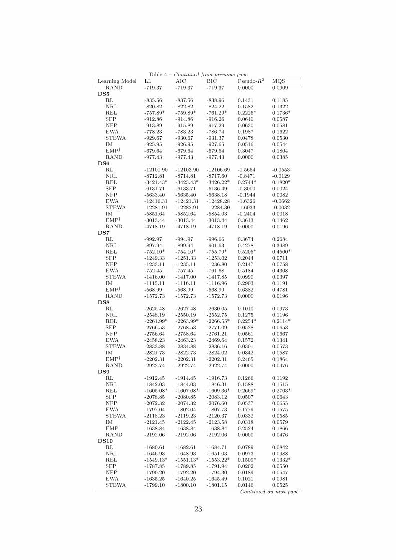
Table 4 – Continued from previous pageLearning Model LL AIC BIC Pseudo-R2 MQS
RAND -719.37 -719.37 -719.37 0.0000 0.0909DS5
RL -835.56 -837.56 -838.96 0.1431 0.1185NRL -820.82 -822.82 -824.22 0.1582 0.1322REL -757.89* -759.89* -761.29* 0.2226* 0.1736*SFP -912.86 -914.86 -916.26 0.0640 0.0587NFP -913.89 -915.89 -917.29 0.0630 0.0581EWA -778.23 -783.23 -786.74 0.1987 0.1622STEWA -929.67 -930.67 -931.37 0.0478 0.0530IM -925.95 -926.95 -927.65 0.0516 0.0544EMP† -679.64 -679.64 -679.64 0.3047 0.1804RAND -977.43 -977.43 -977.43 0.0000 0.0385
DS6RL -12101.90 -12103.90 -12106.69 -1.5654 -0.0553NRL -8712.81 -8714.81 -8717.60 -0.8471 -0.0129REL -3421.43* -3423.43* -3426.22* 0.2744* 0.1820*SFP -6131.71 -6133.71 -6136.49 -0.3000 0.0024NFP -5633.40 -5635.40 -5638.18 -0.1944 0.0082EWA -12416.31 -12421.31 -12428.28 -1.6326 -0.0662STEWA -12281.91 -12282.91 -12284.30 -1.6033 -0.0032IM -5851.64 -5852.64 -5854.03 -0.2404 0.0018EMP† -3013.44 -3013.44 -3013.44 0.3613 0.1462RAND -4718.19 -4718.19 -4718.19 0.0000 0.0196
DS7RL -992.97 -994.97 -996.66 0.3674 0.2684NRL -897.94 -899.94 -901.63 0.4278 0.3489REL -752.10* -754.10* -755.79* 0.5205* 0.4500*SFP -1249.33 -1251.33 -1253.02 0.2044 0.0711NFP -1233.11 -1235.11 -1236.80 0.2147 0.0758EWA -752.45 -757.45 -761.68 0.5184 0.4308STEWA -1416.00 -1417.00 -1417.85 0.0990 0.0397IM -1115.11 -1116.11 -1116.96 0.2903 0.1191EMP† -568.99 -568.99 -568.99 0.6382 0.4781RAND -1572.73 -1572.73 -1572.73 0.0000 0.0196
DS8RL -2625.48 -2627.48 -2630.05 0.1010 0.0973NRL -2548.19 -2550.19 -2552.75 0.1275 0.1196REL -2261.99* -2263.99* -2266.55* 0.2254* 0.2114*SFP -2766.53 -2768.53 -2771.09 0.0528 0.0653NFP -2756.64 -2758.64 -2761.21 0.0561 0.0667EWA -2458.23 -2463.23 -2469.64 0.1572 0.1341STEWA -2833.88 -2834.88 -2836.16 0.0301 0.0573IM -2821.73 -2822.73 -2824.02 0.0342 0.0587EMP† -2202.31 -2202.31 -2202.31 0.2465 0.1864RAND -2922.74 -2922.74 -2922.74 0.0000 0.0476
DS9RL -1912.45 -1914.45 -1916.73 0.1266 0.1192NRL -1842.03 -1844.03 -1846.31 0.1588 0.1515REL -1605.08* -1607.08* -1609.36* 0.2669* 0.2703*SFP -2078.85 -2080.85 -2083.12 0.0507 0.0643NFP -2072.32 -2074.32 -2076.60 0.0537 0.0655EWA -1797.04 -1802.04 -1807.73 0.1779 0.1575STEWA -2118.23 -2119.23 -2120.37 0.0332 0.0585IM -2121.45 -2122.45 -2123.58 0.0318 0.0579EMP -1638.84 -1638.84 -1638.84 0.2524 0.1866RAND -2192.06 -2192.06 -2192.06 0.0000 0.0476
DS10RL -1680.61 -1682.61 -1684.71 0.0789 0.0842NRL -1646.93 -1648.93 -1651.03 0.0973 0.0988REL -1549.13* -1551.13* -1553.22* 0.1509* 0.1332*SFP -1787.85 -1789.85 -1791.94 0.0202 0.0550NFP -1790.20 -1792.20 -1794.30 0.0189 0.0547EWA -1635.25 -1640.25 -1645.49 0.1021 0.0981STEWA -1799.10 -1800.10 -1801.15 0.0146 0.0525
Continued on next page
23
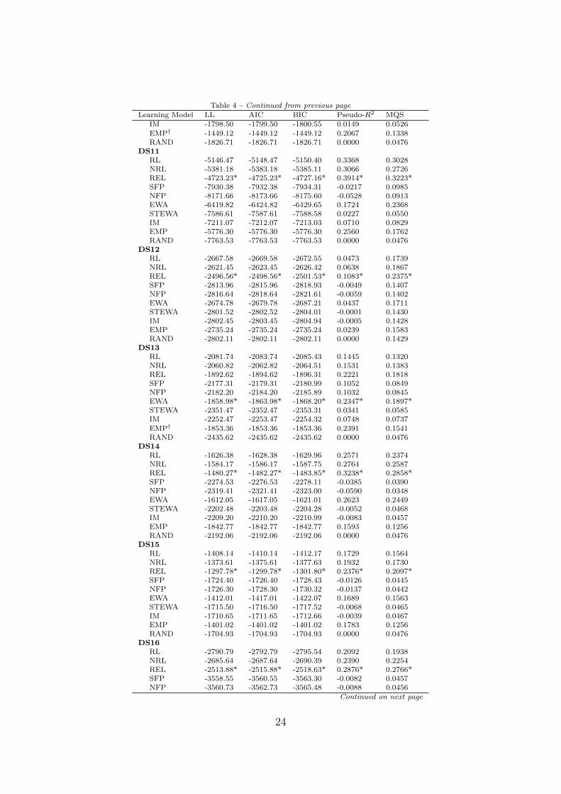
Table 4 – Continued from previous pageLearning Model LL AIC BIC Pseudo-R2 MQS
IM -1798.50 -1799.50 -1800.55 0.0149 0.0526EMP† -1449.12 -1449.12 -1449.12 0.2067 0.1338RAND -1826.71 -1826.71 -1826.71 0.0000 0.0476
DS11RL -5146.47 -5148.47 -5150.40 0.3368 0.3028NRL -5381.18 -5383.18 -5385.11 0.3066 0.2726REL -4723.23* -4725.23* -4727.16* 0.3914* 0.3223*SFP -7930.38 -7932.38 -7934.31 -0.0217 0.0985NFP -8171.66 -8173.66 -8175.60 -0.0528 0.0913EWA -6419.82 -6424.82 -6429.65 0.1724 0.2368STEWA -7586.61 -7587.61 -7588.58 0.0227 0.0550IM -7211.07 -7212.07 -7213.03 0.0710 0.0829EMP -5776.30 -5776.30 -5776.30 0.2560 0.1762RAND -7763.53 -7763.53 -7763.53 0.0000 0.0476
DS12RL -2667.58 -2669.58 -2672.55 0.0473 0.1739NRL -2621.45 -2623.45 -2626.42 0.0638 0.1867REL -2496.56* -2498.56* -2501.53* 0.1083* 0.2375*SFP -2813.96 -2815.96 -2818.93 -0.0049 0.1407NFP -2816.64 -2818.64 -2821.61 -0.0059 0.1402EWA -2674.78 -2679.78 -2687.21 0.0437 0.1711STEWA -2801.52 -2802.52 -2804.01 -0.0001 0.1430IM -2802.45 -2803.45 -2804.94 -0.0005 0.1428EMP -2735.24 -2735.24 -2735.24 0.0239 0.1583RAND -2802.11 -2802.11 -2802.11 0.0000 0.1429
DS13RL -2081.74 -2083.74 -2085.43 0.1445 0.1320NRL -2060.82 -2062.82 -2064.51 0.1531 0.1383REL -1892.62 -1894.62 -1896.31 0.2221 0.1818SFP -2177.31 -2179.31 -2180.99 0.1052 0.0849NFP -2182.20 -2184.20 -2185.89 0.1032 0.0845EWA -1858.98* -1863.98* -1868.20* 0.2347* 0.1897*STEWA -2351.47 -2352.47 -2353.31 0.0341 0.0585IM -2252.47 -2253.47 -2254.32 0.0748 0.0737EMP† -1853.36 -1853.36 -1853.36 0.2391 0.1541RAND -2435.62 -2435.62 -2435.62 0.0000 0.0476
DS14RL -1626.38 -1628.38 -1629.96 0.2571 0.2374NRL -1584.17 -1586.17 -1587.75 0.2764 0.2587REL -1480.27* -1482.27* -1483.85* 0.3238* 0.2858*SFP -2274.53 -2276.53 -2278.11 -0.0385 0.0390NFP -2319.41 -2321.41 -2323.00 -0.0590 0.0348EWA -1612.05 -1617.05 -1621.01 0.2623 0.2449STEWA -2202.48 -2203.48 -2204.28 -0.0052 0.0468IM -2209.20 -2210.20 -2210.99 -0.0083 0.0457EMP -1842.77 -1842.77 -1842.77 0.1593 0.1256RAND -2192.06 -2192.06 -2192.06 0.0000 0.0476
DS15RL -1408.14 -1410.14 -1412.17 0.1729 0.1564NRL -1373.61 -1375.61 -1377.63 0.1932 0.1730REL -1297.78* -1299.78* -1301.80* 0.2376* 0.2097*SFP -1724.40 -1726.40 -1728.43 -0.0126 0.0445NFP -1726.30 -1728.30 -1730.32 -0.0137 0.0442EWA -1412.01 -1417.01 -1422.07 0.1689 0.1563STEWA -1715.50 -1716.50 -1717.52 -0.0068 0.0465IM -1710.65 -1711.65 -1712.66 -0.0039 0.0467EMP -1401.02 -1401.02 -1401.02 0.1783 0.1256RAND -1704.93 -1704.93 -1704.93 0.0000 0.0476
DS16RL -2790.79 -2792.79 -2795.54 0.2092 0.1938NRL -2685.64 -2687.64 -2690.39 0.2390 0.2254REL -2513.88* -2515.88* -2518.63* 0.2876* 0.2766*SFP -3558.55 -3560.55 -3563.30 -0.0082 0.0457NFP -3560.73 -3562.73 -3565.48 -0.0088 0.0456
Continued on next page
24
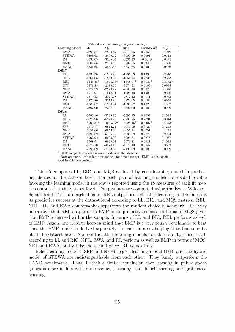
Table 4 – Continued from previous pageLearning Model LL AIC BIC Pseudo-R2 MQS
EWA -2799.87 -2804.87 -2811.75 0.2058 0.1919STEWA -3498.62 -3499.62 -3500.99 0.0091 0.0523IM -3534.05 -3535.05 -3536.43 -0.0010 0.0475EMP -2704.55 -2704.55 -2704.55 0.2342 0.1620RAND -3531.65 -3531.65 -3531.65 0.0000 0.0476
DS17RL -1933.20 -1935.20 -1936.89 0.1930 0.2340NRL -1861.05 -1863.05 -1864.74 0.2230 0.2673REL -1644.38* -1646.38* -1648.07* 0.3134* 0.3372*SFP -2371.23 -2373.23 -2374.91 0.0103 0.0994NFP -2377.79 -2379.79 -2381.48 0.0076 0.1016EWA -1913.91 -1918.91 -1923.13 0.1998 0.2370STEWA -2370.28 -2371.28 -2372.12 0.0111 0.0963IM -2372.80 -2373.80 -2374.65 0.0100 0.0959EMP -1960.87 -1960.87 -1960.87 0.1823 0.1907RAND -2397.90 -2397.90 -2397.90 0.0000 0.0909
DS18RL -5586.16 -5588.16 -5590.95 0.2232 0.2543NRL -5226.96 -5228.96 -5231.75 0.2731 0.3044REL -4093.37* -4095.37* -4098.16* 0.4307* 0.4393*SFP -6670.77 -6672.77 -6675.56 0.0724 0.1258NFP -6651.66 -6653.66 -6656.44 0.0751 0.1275EWA -5190.02 -5195.02 -5201.99 0.2778 0.2964STEWA -6992.92 -6993.92 -6995.31 0.0278 0.1037IM -6968.91 -6969.91 -6971.31 0.0311 0.1052EMP -4570.10 -4570.10 -4570.10 0.3647 0.3653RAND -7193.69 -7193.69 -7193.69 0.0000 0.0909
† EMP outperforms all learning models in this data set.∗ Best among all other learning models for this data set. EMP is not consid-ered in this comparison.
Table 5 compares LL, BIC, and MQS achieved by each learning model in predict-ing choices at the dataset level. For each pair of learning models, one sided p-valuefavoring the learning model in the row is reported using the 18 measures of each fit met-ric computed at the dataset level. The p-values are computed using the Exact WilcoxonSigned-Rank Test for matched pairs. REL outperforms all other learning models in termsits predictive success at the dataset level according to LL, BIC, and MQS metrics. REL,NRL, RL, and EWA comfortably outperform the random choice benchmark. It is veryimpressive that REL outperforms EMP in its predictive success in terms of MQS giventhat EMP is derived within the sample. In terms of LL and BIC, REL performs as wellas EMP. Again, one need to keep in mind that EMP is a very tough benchmark to beatsince the EMP model is derived separately for each data set helping it to fine tune itsfit at the dataset level. None of the other learning models are able to outperform EMPaccording to LL and BIC. NRL, EWA, and RL perform as well as EMP in terms of MQS.NRL and EWA jointly take the second place. RL comes third.
Belief learning models (SFP and NFP), regret learning model (IM), and the hybridmodel of STEWA are indistinguishable from each other. They barely outperform theRAND benchmark. Thus, I reach a similar conclusion that learning in public goodsgames is more in line with reinforcement learning than belief learning or regret basedlearning.
25

Table 5: Comparison of predictive accuracy of learning models. For each pair oflearning models, one sided p-value favoring the learning model in the row is reportedusing the 18 measures of each fit metric computed at the dataset level. The p-valuesare computed using the Exact Wilcoxon Signed-Rank Test for matched pairs.
EMP NRL EWA RL NFP SFP IM STEWA RAND
RELLL 0.3669 0.0000 0.0000 0.0000 0.0000 0.0000 0.0000 0.0000 0.0000BIC 0.3994 0.0000 0.0000 0.0000 0.0000 0.0000 0.0000 0.0000 0.0000MQS 0.0002 0.0000 0.0000 0.0000 0.0000 0.0000 0.0000 0.0000 0.0000
EMPLL 0.0269 0.0028 0.0091 0.0000 0.0000 0.0000 0.0000 0.0000BIC 0.0269 0.0028 0.0091 0.0000 0.0000 0.0000 0.0000 0.0000MQS 0.6170 0.6953 0.2899 0.0000 0.0000 0.0000 0.0000 0.0000
NRLLL 0.5169 0.0008 0.0010 0.0010 0.0010 0.0000 0.0010BIC 0.3994 0.0008 0.0010 0.0010 0.0010 0.0000 0.0010MQS 0.2341 0.0003 0.0000 0.0000 0.0000 0.0000 0.0000
EWALL 0.0333 0.0010 0.0010 0.0010 0.0000 0.0010BIC 0.0708 0.0010 0.0010 0.0010 0.0000 0.0010MQS 0.0104 0.0000 0.0000 0.0000 0.0000 0.0000
RLLL 0.0010 0.0010 0.0010 0.0000 0.0010BIC 0.0010 0.0010 0.0010 0.0000 0.0010MQS 0.0001 0.0001 0.0000 0.0000 0.0000
NFPLL 0.4493 0.5841 0.3994 0.1144BIC 0.4493 0.6331 0.4325 0.1519MQS 0.2899 0.3353 0.0982 0.0060
SFPLL 0.7914 0.3830 0.0770BIC 0.8376 0.3994 0.0982MQS 0.3509 0.1061 0.0069
IMLL 0.1733 0.0080BIC 0.1733 0.0104MQS 0.0837 0.0033
STEWALL 0.0024BIC 0.0028MQS 0.0024
Notes:
LL - Log-Likelihood
BIC - Bayesian Information Criterion
MQS - Mean Quadratic Score
EMP is the model based on empirical frequencies of strategies within each dataset. Note that the empiricalfrequencies are derived at the dataset level and not the pooled data level. This is because the number ofstrategies available to individuals are not identical across datasets due to varying levels of endowment.
RAND is the random choice model derived at the dataset level. This is because the number of strategiesavailable to individuals are not identical across datasets due to varying levels of endowment.
26
6 Discussion
6.1 EWA Overfits and REL Generalizes Well
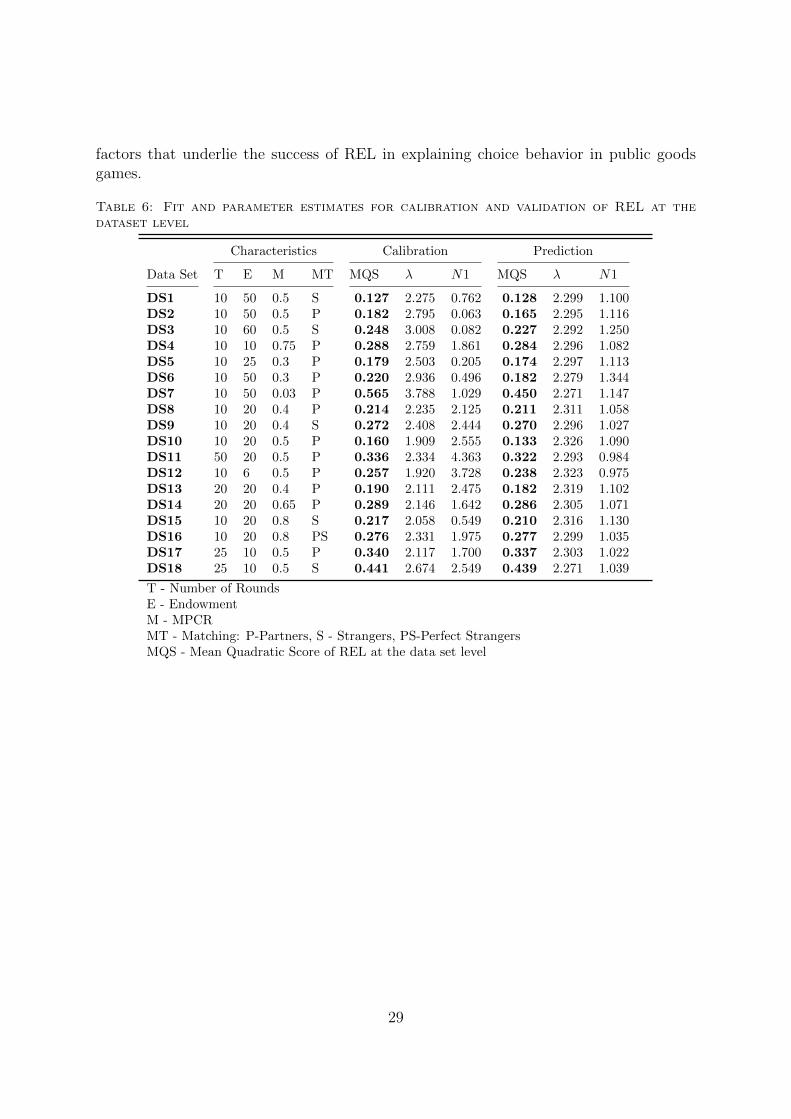
In this subsection I discuss the factors that contribute to REL’s success in its descriptivesuccess and predictive accuracy. First, I compare it side by side with EWA which doesnot do as as well. Among the learning models that are considered in this paper, EWAis the most flexible model since it has free parameters that help it to adjust the rate ofdiscounting previous attractions using φ, type of learning (i.e. reinforcement or beliefbased or a mix of the two) using δ, the type of attraction updating (i.e. cumulativeor averaging) using the parameter κ. Despite all the flexibility it has, it does not fareas well as REL. To gain insight into what is behind the superior performance of RELcompared to EWA in its generalizability, I fit these two models at the data set level.Under Calibration in Table 6, the parameter values that maximized log-likelihood of agiven dataset are reported for the REL Model. Under Prediction in Table 6, the parametervalues that maximized log-likelihood across the 17 datasets other than a given dataset arereported. These are the parameters that were used to predict the choices in the dataset inSection 5.2. MQS values achieved in calibration and prediction are also reported. Table7 presents parameter estimates and MQS achieved for both calibration and predictionfor EWA model. The parameters in the calibration of EWA help it to fit the choices ineach dataset separately giving it a much better chance in fitting the data due to its highdegrees of freedom. Indeed, when we compare the MQSs achieved by EWA and RELat the dataset level calibration, EWA outperforms REL (Exact Wilcoxon Signed-RankTest: p < 0.001). However, as we noted in the Results section 5.2, in prediction RELoutperforms EWA (Exact Wilcoxon Sign-Rank Test: p < 0.001). This highlights theproblem with EWA: it overfits the data.
The parameter values for REL are very close in both calibration and prediction for alldatasets helping it to achieve very close performance in both calibration and prediction.Note that one cannot achieve a better fit than the fit achieved in calibration. However, inthe context of EWA, there are significant differences in the estimated parameter valuesin calibration and prediction. Since the parameters used for prediction are way far awayfrom the calibration parameters that lead to the maximum possible likelihood using thelearning model (the log-likelihood in calibration), the achieved prediction MQS valuesare quite low.
The most important parameters in EWA learning model are the rate of forgettingparameter φ, the aspiration level parameter δ that determines the type of learning, andκ that determines whether attractions are updated cumulatively or by averaging. Table7 shows that large discrepancies are occurring in terms of κ and δ between the calibratedparameters and prediction parameters. κ’s used for prediction are closer to 1 meaningattraction updating is cumulative, but the calibrated parameter values are significantlysmaller indicating that learning that achieves the best fit is actually closer to an averagingattraction updating model. Similarly, the prediction δ values lean towards more of belieflearning (δ = 1 indicates pure belief learning and δ = 0 indicates pure reinforcement
27
learning). However, for many data sets (for example DS6, DS15, DS16), the calibrated δis very close to 0 indicating the learning that explains the data in those datasets is muchcloser to that of reinforcement learning. The parameters that are used for prediction arevery close the parameters that maximized log-likelihood for the pooled data reported inTable 2, which makes sense because these parameters were estimated with 17 of the 18datasets. The take away from the comparison of calibration and prediction parameters ofEWA is that the model parameters need to be adjusted significantly based on the gameparameters to explain behavior and it has a hard time finding one set of parametersthat can describe well the behavior across public goods games with a wide range ofparameters. Such discrepancies between the parameters estimated using pooled data andthe parameters estimated at the individual dataset level are also reported in Erev andHaruvy (2005). These results demonstrate how easy it is to run into overfitting problemswhen studying learning in games. For example, if we take any of the 18 datasets inisolation, EWA achieves significantly better performance than REL in fitting the data,therefore one may have to conclude learning is more in line with that of EWA. We are onlyable to identify the overfitting problem of EWA by studying its performance in describingand predicting choices in multiple datasets that have data on public goods games with awide ranging parameters.
There are two components in REL that set it apart from other models in the rein-forcement family: adaptive attraction sensitivity that decreases with increasing payoffvariability and its insensitivity to payoff magnitude. By comparing RL and NRL, onecan conclude that adaptive attraction sensitivity that decreases with increasing payoffvariability is important in explaining choice behavior in public goods environment. NRLis identical to RL but has an adaptive attraction sensitivity and achieves a significantlybetter performance in both descriptive fit and predictive accuracy. Apart from very mi-nor specification details, both REL and NRL are identical in that they both use averagechoice reinforcement and both employ an adaptive attraction sensitivity that decreaseswith increasing payoff variability. Here, I assess if REL’s insensitivity to payoff magni-tude puts it ahead of NRL. REL achieves insensitivity to payoff magnitude by scaling theattraction sensitivity parameter (λ) by baseline payoff variability that is computed basedon a random choice in the first round. Therefore, first round’s effective attraction sensi-tivity is λ/PV 1. For example, in DS1 where E = 50 and M = 0.5, PV1 is 26.07. Whereasin DS4 where E = 10 and M = 0.75, PV1 is 18.47. First round effective attraction sensi-tivity of the REL learning model will be different for individuals in these two data sets.In contrast, NRL’s first round payoff variability is initialized as PV 1 = λ. This makes theeffective attraction sensitivity, λ/PV 1, equal to 1 in any dataset irrespective of E or M.Thus, in NRL learning will be sensitive to payoff magnitudes in the game which dependupon the game’s E and M. To evaluate how much REL’s payoff magnitude insensitivitycontribute to its success , I estimate a variation of REL model where I initialize PV 1 = λmaking the first round effective attraction sensitivity equal to 1 as in NRL. The resultingmodel indeed performs significantly worse than the original REL (Likelihood Ratio Test,χ2 = 842, p < 0.0001). I conclude that both adaptive attraction sensitivity that scaleswith payoff variability and leaning that is insensitive to payoff magnitudes are important
28
factors that underlie the success of REL in explaining choice behavior in public goodsgames.
Table 6: Fit and parameter estimates for calibration and validation of REL at thedataset level
Characteristics Calibration Prediction
Data Set T E M MT MQS λ N1 MQS λ N1
DS1 10 50 0.5 S 0.127 2.275 0.762 0.128 2.299 1.100DS2 10 50 0.5 P 0.182 2.795 0.063 0.165 2.295 1.116DS3 10 60 0.5 S 0.248 3.008 0.082 0.227 2.292 1.250DS4 10 10 0.75 P 0.288 2.759 1.861 0.284 2.296 1.082DS5 10 25 0.3 P 0.179 2.503 0.205 0.174 2.297 1.113DS6 10 50 0.3 P 0.220 2.936 0.496 0.182 2.279 1.344DS7 10 50 0.03 P 0.565 3.788 1.029 0.450 2.271 1.147DS8 10 20 0.4 P 0.214 2.235 2.125 0.211 2.311 1.058DS9 10 20 0.4 S 0.272 2.408 2.444 0.270 2.296 1.027DS10 10 20 0.5 P 0.160 1.909 2.555 0.133 2.326 1.090DS11 50 20 0.5 P 0.336 2.334 4.363 0.322 2.293 0.984DS12 10 6 0.5 P 0.257 1.920 3.728 0.238 2.323 0.975DS13 20 20 0.4 P 0.190 2.111 2.475 0.182 2.319 1.102DS14 20 20 0.65 P 0.289 2.146 1.642 0.286 2.305 1.071DS15 10 20 0.8 S 0.217 2.058 0.549 0.210 2.316 1.130DS16 10 20 0.8 PS 0.276 2.331 1.975 0.277 2.299 1.035DS17 25 10 0.5 P 0.340 2.117 1.700 0.337 2.303 1.022DS18 25 10 0.5 S 0.441 2.674 2.549 0.439 2.271 1.039
T - Number of RoundsE - EndowmentM - MPCRMT - Matching: P-Partners, S - Strangers, PS-Perfect StrangersMQS - Mean Quadratic Score of REL at the data set level
29
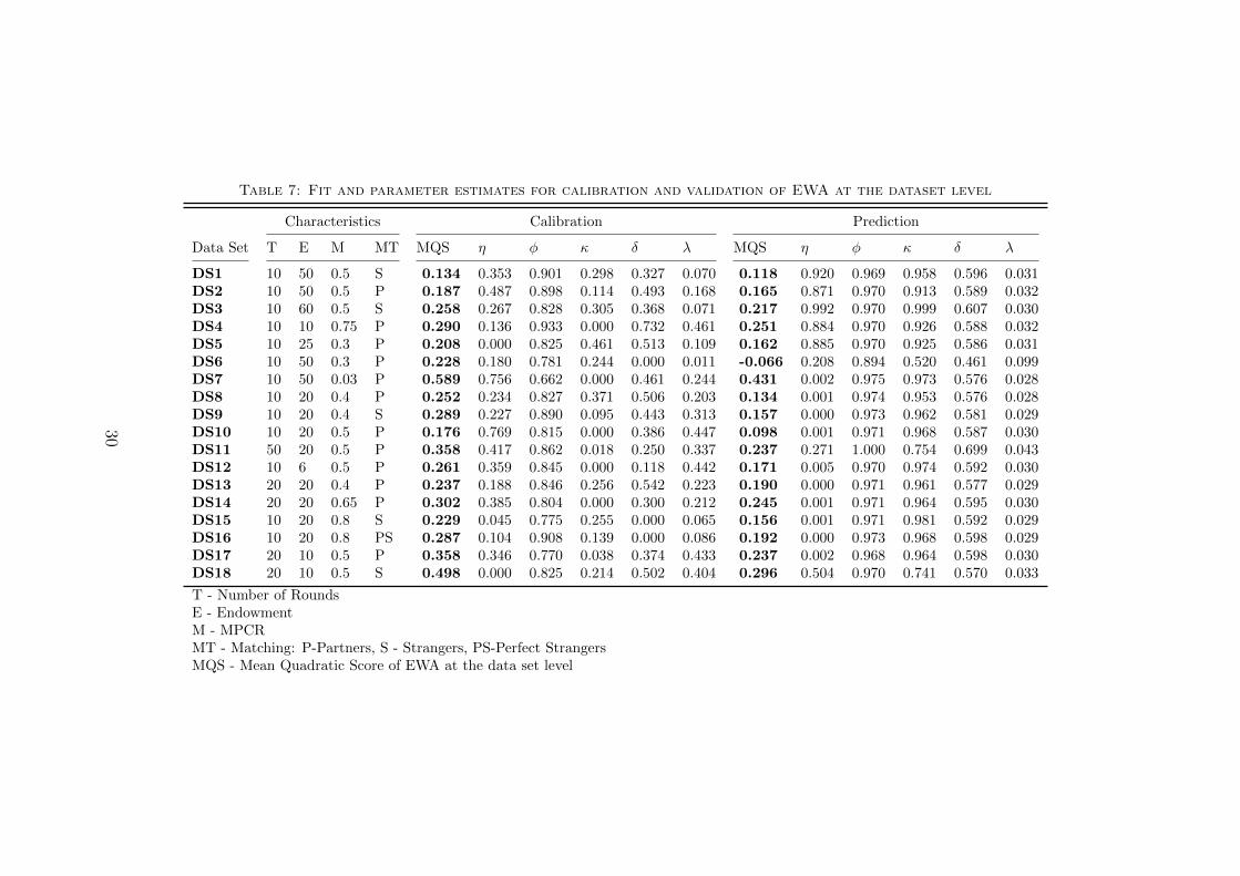
Table 7: Fit and parameter estimates for calibration and validation of EWA at the dataset level
Characteristics Calibration Prediction
Data Set T E M MT MQS η φ κ δ λ MQS η φ κ δ λ
DS1 10 50 0.5 S 0.134 0.353 0.901 0.298 0.327 0.070 0.118 0.920 0.969 0.958 0.596 0.031DS2 10 50 0.5 P 0.187 0.487 0.898 0.114 0.493 0.168 0.165 0.871 0.970 0.913 0.589 0.032DS3 10 60 0.5 S 0.258 0.267 0.828 0.305 0.368 0.071 0.217 0.992 0.970 0.999 0.607 0.030DS4 10 10 0.75 P 0.290 0.136 0.933 0.000 0.732 0.461 0.251 0.884 0.970 0.926 0.588 0.032DS5 10 25 0.3 P 0.208 0.000 0.825 0.461 0.513 0.109 0.162 0.885 0.970 0.925 0.586 0.031DS6 10 50 0.3 P 0.228 0.180 0.781 0.244 0.000 0.011 -0.066 0.208 0.894 0.520 0.461 0.099DS7 10 50 0.03 P 0.589 0.756 0.662 0.000 0.461 0.244 0.431 0.002 0.975 0.973 0.576 0.028DS8 10 20 0.4 P 0.252 0.234 0.827 0.371 0.506 0.203 0.134 0.001 0.974 0.953 0.576 0.028DS9 10 20 0.4 S 0.289 0.227 0.890 0.095 0.443 0.313 0.157 0.000 0.973 0.962 0.581 0.029DS10 10 20 0.5 P 0.176 0.769 0.815 0.000 0.386 0.447 0.098 0.001 0.971 0.968 0.587 0.030DS11 50 20 0.5 P 0.358 0.417 0.862 0.018 0.250 0.337 0.237 0.271 1.000 0.754 0.699 0.043DS12 10 6 0.5 P 0.261 0.359 0.845 0.000 0.118 0.442 0.171 0.005 0.970 0.974 0.592 0.030DS13 20 20 0.4 P 0.237 0.188 0.846 0.256 0.542 0.223 0.190 0.000 0.971 0.961 0.577 0.029DS14 20 20 0.65 P 0.302 0.385 0.804 0.000 0.300 0.212 0.245 0.001 0.971 0.964 0.595 0.030DS15 10 20 0.8 S 0.229 0.045 0.775 0.255 0.000 0.065 0.156 0.001 0.971 0.981 0.592 0.029DS16 10 20 0.8 PS 0.287 0.104 0.908 0.139 0.000 0.086 0.192 0.000 0.973 0.968 0.598 0.029DS17 20 10 0.5 P 0.358 0.346 0.770 0.038 0.374 0.433 0.237 0.002 0.968 0.964 0.598 0.030DS18 20 10 0.5 S 0.498 0.000 0.825 0.214 0.502 0.404 0.296 0.504 0.970 0.741 0.570 0.033
T - Number of RoundsE - EndowmentM - MPCRMT - Matching: P-Partners, S - Strangers, PS-Perfect StrangersMQS - Mean Quadratic Score of EWA at the data set level
30
6.2 Comparison of REL with Individual Evolutionary Learning
There is one thing that is common among the learning models that are considered so far inthis paper. All of them are based on interpretable cognitive or psychological mechanismsthat were put forward by decades of experimental research on humans and animals. Forexample, the idea of reinforcing actions that led to higher payoffs in the previous roundsof play with higher probabilities is one of the simplest and oldest of learning models andits origins can be traced to the psychological learning theories of Luce (2005), Thurstone(1930) and Bush and Mosteller (1955). Thus, learning models considered until now rankhigh in terms of cognitive plausibility. On the other end of the spectrum are learningmodels based on the template of evolution. These models are often hard to interpretin terms of underlying cognitive or neural mechanism substrates. A number of papershave considered if evolutionary learning models can provide a successful account of theoutcomes in linear public goods games. For example see Clemens and Riechmann (2006);Miller and Andreoni (1991); Arifovic and Ledyard (2012).
In this subsection, I compare the Individual Evolutionary Learning (IEL) model putforward by Arifovic and Ledyard (2012) with REL model in its ability to explain con-tribution patterns observed in the data considered in this paper Arifovic and Ledyard(2012) have shown that IEL in conjunction with their social preference model can explainmany observed regularities in repeated public goods games. To put IEL and REL on thesame footing, in this paper I do not consider social preferences in conjunction with IEL.A brief description of IEL learning model is provided in Appendix 8. There are two freeparameters in IEL model: memory size (J), experimentation probability (ρ). J denotesthe size of the set of strategies an individual remembers and ρ determines the probabil-ity with which each strategy in the memory of an individual gets replaced by a randomstrategy that is picked from all available strategies.
Standard econometric methods like maximum likelihood estimation are difficult touse with IEL since it induces a Markov process on the sets of actions rather than onindividual actions. Therefore, I use simulation methods to compare IEL with REL interms of how closely they fit the distribution of choices in the data.
Since the decision making process in the learning models is stochastic, I conduct 100simulations per dataset and derive a measure of how close the simulated contributions areto the observed contributions. One way to evaluate the closeness of observed contribu-tions and simulated contributions is to compare the average contributions in simulationswith the average contributions observed in each dataset over the rounds. First averagecontribution in each round is computed in each simulation run to derive the path of av-erage contributions. These simulated paths of average contributions over 100 simulationare averaged to obtain the representative path of average contributions. One can thencompute the distance between the computed path of average contributions with the ac-tual path of average contributions in the dataset. This distance measure average over 18data sets would give a measure of how successful a learning model is in generating theaverage contributions that are closer to the observed average contributions. This is theapproach taken by a number of previous papers in evaluating learning models (Deadman,1999; Janssen & Ahn, 2006; Castillo & Saysel, 2005). However, contributions in public
31
good experiments are consistently observed to be multi modal with generally three peaksat zero, half endowment, and full endowment(Ledyard, 1995). While contributions de-crease over time, multi modal nature of them persists. Thus a model that produces avery close pattern of average contributions over time might not necessarily capture thedistributional aspect of the contributions well. In light of this, a good model should bethe one that generates a distribution of contributions in each round that is close to thedistribution of observed contributions in that round. I characterize the similarity betweenthe distribution of choices simulated by a learning model in a round with the distributionof the observed choices using two distributional distance measures. I use two measures,since it was observed in previous literature that different choices of distance measures canlead to different conclusions in model selection (Feltovich, 2000). To guard the analysisfrom such an occurrence here, I use two distance measures to compare REL and IEL.
To compare how well IEL and REL generate contributions that are closer to theobserved contributions, I use two distributional distance measures. A number of dis-tance metrics are proposed to measure the distance between two probability distribu-tions. The Kullback-Leibler (KL) divergence and Pearson’s-χ2 divergence are two of thewell-known such metrics. A particular concern in using these widely used metrics is thatthey are asymmetric. To circumvent this problem, I use symmetric versions of thesedivergence measures: Jensen-Shannon divergence (Lin, 1991) is a symmetric extension ofKullback-Leibler (KL) divergence and Probabilistic Symmetric−χ2 (Deza & Deza, 2006)is a symmetric variation of the Pearson’s-χ2. Say the empirical discrete distribution ofthe observed contributions in a given round is P and the empirical discrete distributionof the simulated choices in the round is Q. If E is the endowment, there are E+ 1 strate-gies (discrete contribution levels from 0 to E.). The two distance measures can then bedefined as:
1. Probabilistic Symmetric−χ2 distance:
dχ2 = 2E∑j=0
(Pj −Qj)2
Pj +Qj
2. Jensen-Shannon divergence:
dJS =1
2
[ E∑j=0
Pjln
(2Pj
Pj +Qj
)+
E∑j=0
Qjln
(2Qj
Pj +Qj
)]
For REL and IEL, I compute the distance measures for each of the 18 datasets usingsimulation. I take an average of the dataset level distance measures as the overall measureof distance between the simulated and observed contributions. I conduct a grid search tofind the values of learning parameters that minimize the distances for each model. ForREL, I varied λ from 0 to 4 in increments of 0.1 and varied N1 from 0 to 10 in incrementsof 1. For IEL, I varied J from 50 to 200 in increments of 10 and varied ρ from 0 to 1 inincrements of 0.02. Achieved distance measures over the corresponding grids are shown in
32
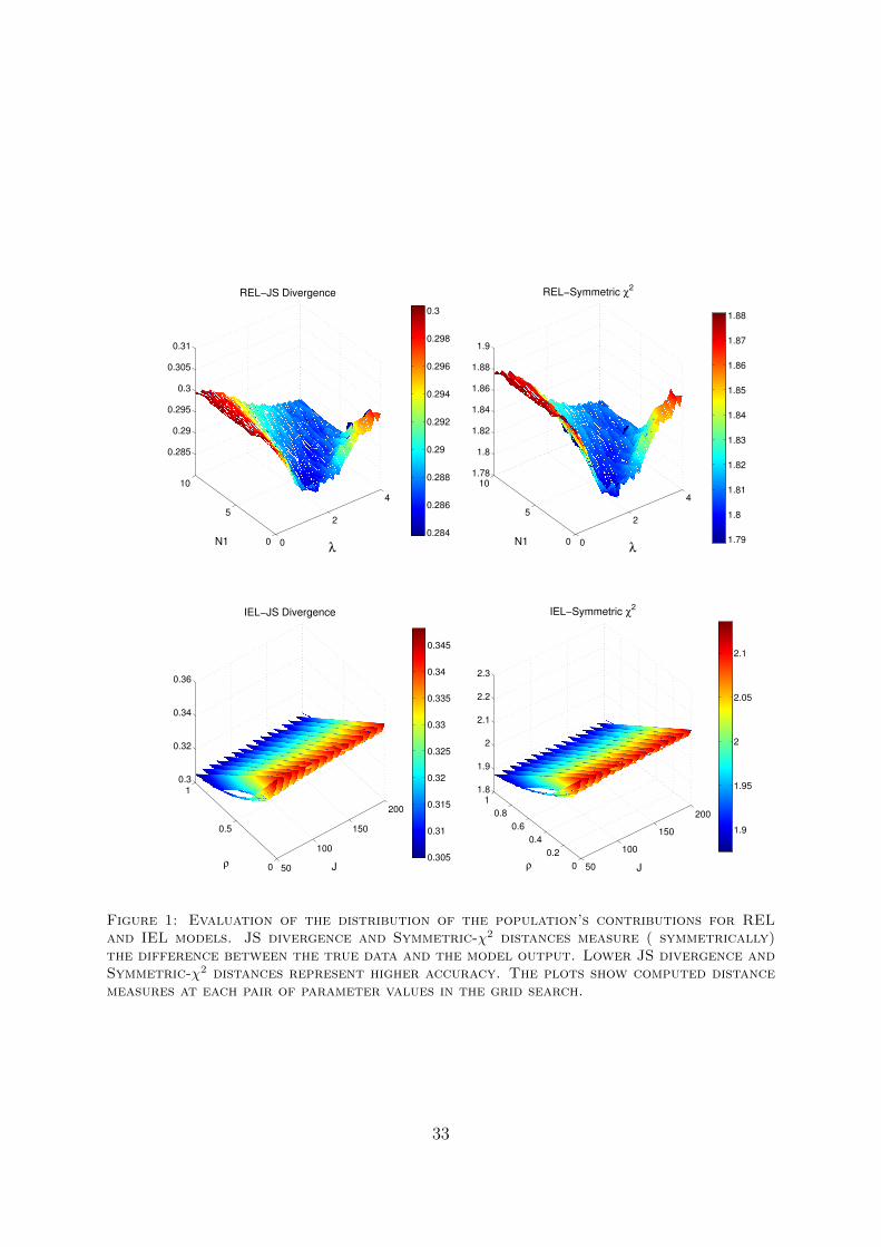
0
2
4
0
5
10
0.285
0.29
0.295
0.3
0.305
0.31
λ
REL−JS Divergence
N1 0.284
0.286
0.288
0.29
0.292
0.294
0.296
0.298
0.3
0
2
4
0
5
101.78
1.8
1.82
1.84
1.86
1.88
1.9
λ
REL−Symmetric χ2
N1
1.79
1.8
1.81
1.82
1.83
1.84
1.85
1.86
1.87
1.88
50
100
150
200
0
0.5
10.3
0.32
0.34
0.36
J
IEL−JS Divergence
ρ 0.305
0.31
0.315
0.32
0.325
0.33
0.335
0.34
0.345
50
100
150
200
0
0.2
0.4
0.6
0.8
11.8
1.9
2
2.1
2.2
2.3
J
IEL−Symmetric χ2
ρ
1.9
1.95
2
2.05
2.1
Figure 1: Evaluation of the distribution of the population’s contributions for RELand IEL models. JS divergence and Symmetric-χ2 distances measure ( symmetrically)the difference between the true data and the model output. Lower JS divergence andSymmetric-χ2 distances represent higher accuracy. The plots show computed distancemeasures at each pair of parameter values in the grid search.
33
Table 8: Evaluation of the distribution of the population’s contributions for REL andIEL models. JS divergence and Symmetric-χ2 measure ( symmetrically) the distancebetween the true data and the model output. Lower JS divergence and Symmetric-χ2
distances represent higher accuracy. Reported are the minimum distances achieved byeach model.
JS-Divergence Symmetric-χ2
Model Parameters dJS Parameters dχ2
REL λ = 1.9, N1 = 2 0.2838 λ = 1.9, N1 = 2 1.7885
IEL J = 50, ρ = 1 0.3048 J = 50, ρ = 1 1.8750
Figure 1 for both models. The smallest distances achieved for two models are presentedin Table 8. REL outperforms IEL in predicting the full distribution of contributions overrounds. From Figure 1 it can be noted that IEL performs better for high values of ρ. Thebest score achieved by IEL is for ρ = 1 which means that every strategy in the memoryis replaced by a random strategy with a probability of 1 in each round. REL does betterthan a random choice model since the best score REL achieves is better than what itachieves when λ = 0 (when λ = 0, REL is equivalent to the random choice model). Iconclude that REL outperforms IEL in predicting full distribution of contributions.
7 Conclusions
In this paper, the models of reinforcement learning (RL), normalized reinforcement learn-ing (NRL), reinforcement average model with loss aversion strategy (REL), stochasticfictitious play (SFP), normalized stochastic fictitious play (NFP), experience weightedattraction learning (EWA), self-tuning EWA (STEWA), and impulse matching learning(IM) were applied and tested in the environment of public goods games with a wide rang-ing game parameters. Experimental data from 12 published studies was used to construct18 datasets each of which is different from the remaining in at least one the public goodsgame parameters: marginal per capita return, group size, number of rounds, endowment,and matching protocol. Learning models were compared on the basis of their descriptivefit and prediction accuracy.
The main finding in this study is that REL outperforms all other learning models interms of both descriptive fit and prediction accuracy. It is the only model to outperformdataset level overall empirical frequencies in both descriptive fit and predictive accuracywhen model performance is compared using Mean Quadratic Score (MQS). In terms oflog-likelihood (LL) and BIC, REL performs as well as the dataset level overall empiricalfrequencies in both comparisons. None of the remaining models out-perform the datasetlevel overall empirical frequencies in both comparisons according to any of the metrics.EWA and NRL jointly take the second place. They are outperformed by the dataset leveloverall empirical frequencies in terms of LL and BIC. But, they do as well as the dataset
34
level overall empirical frequencies in terms of MQS. The ordering of learning models inboth comparisons is identical: REL, NRL, EWA, RL, NSFP, SFP, IM, STEWA (the or-dering is not strict in all cases. REL performs strictly better than all other models). RELalso outperforms individual evolutionary learning (IEL) in predicting full distribution ofcontributions.
The results in this paper suggest that belief learning models and regret-based learningmodels perform poorly in comparison to reinforcement models in public goods environ-ments. Learning in public goods games appears to be more in line with reinforcementlearning. Average reinforcement learning that is adaptive to observed payoff variabilityand insensitive to the payoff magnitude underlies the success of REL. These results standin stark contrast to the results from studies with 2×2 games. For example, Chmura et al.(2012) finds that regret-based models and belief learning models out-perform reinforce-ment learning models in explaining data from twelve 2×2 games that cover both constantsum and non-constant sum games. One potential reason for the success of reinforcementlearning models in public goods games could be that individuals perceive public goodsenvironments being too complex and thus resort to simple experience based reinforcementlearning model rather than much more complex belief learning or regret-based learning.
There could be two additional potential reasons behind the failure of belief basedand regret-based learning models in linear public goods environments. First, in the basicpublic goods game setting, these models imply a faster learning of the Nash equilibriumcontribution which is zero. Thus contributions drop very fast to near zero. This alsohappens with IEL model without social preferences. But in the data, the movementtowards zero is slow and contributions in the later rounds of a repeated game are multi-modal with a non-trivial probability mass at non-zero contribution levels. Second, it ispossible that individuals could be forming beliefs in a way very different from that ofwhat is captured in the belief learning models like SFP and NFP. In my follow up papers,I evaluate if belief learning models can perform better at explaining public goods gamedata when they are combined with a model of social preferences. Social preferences helpthe learning models not to drop to zero contributions since multiple Nash equilibria arepossible and not all of them involve zero contributions. I also study if elicited beliefscapture the learning much more accurately than the beliefs modeled by prominent belieflearning models. To do so, I conduct experiments where I elicit beliefs of individuals ineach round of a repeated public goods game in an incentive compatible manner.
References
Andreoni, J. (1988). Why free ride?: Strategies and learning in public goods experiments.Journal of Public Economics , 37 (3), 291–304.
Andreoni, J. (1995a). Cooperation in public-goods experiments: kindness or confusion?The American Economic Review , 891–904.
Andreoni, J. (1995b). Warm-glow versus cold-prickle: the effects of positive and negativeframing on cooperation in experiments. The Quarterly Journal of Economics , 1–21.
35
Arifovic, J., & Ledyard, J. (2012). Individual evolutionary learning, other-regarding pref-erences, and the voluntary contributions mechanism. Journal of Public Economics ,96 (9), 808–823.
Arthur, W. B. (1991). Designing economic agents that act like human agents: A be-havioral approach to bounded rationality. The American Economic Review , 81 (2),353–359.
Botelho, A., Harrison, G. W., Pinto, L. M. C., & Rutstrom, E. E. (2009). Testing staticgame theory with dynamic experiments: a case study of public goods. Games andEconomic behavior , 67 (1), 253–265.
Brier, G. W. (1950). Verification of forecasts expressed in terms of probability. Monthlyweather review , 78 (1), 1–3.
Bush, R. R., & Mosteller, F. (1955). Stochastic models for learning.Camerer, C., & Ho, T.-H. (1999). Experience-weighted attraction learning in normal
form games. Econometrica, 67 , 827–874.Castillo, D., & Saysel, A. K. (2005). Simulation of common pool resource field ex-
periments: a behavioral model of collective action. Ecological economics , 55 (3),420–436.
Cheung, Y.-W., & Friedman, D. (1997). Individual learning in normal form games: Somelaboratory results. Games and Economic Behavior , 19 (1), 46–76.
Chmura, T., Goerg, S. J., & Selten, R. (2012). Learning in experimental 2× 2 games.Games and Economic Behavior , 76 (1), 44–73.
Clemens, C., & Riechmann, T. (2006). Evolutionary dynamics in public good games.Computational Economics , 28 (4), 399–420.
Cooper, D. J., Garvin, S., & Kagel, J. H. (1997). Signalling and adaptive learning in anentry limit pricing game. The RAND Journal of Economics , 662–683.
Cooper, D. J., & Stockman, C. K. (2002). Fairness and learning: an experimentalexamination. Games and Economic Behavior , 41 (1), 26–45.
Cross, J. G., et al. (2008). A theory of adaptive economic behavior. Cambridge Books .Deadman, P. J. (1999). Modelling individual behaviour and group performance in an
intelligent agent-based simulation of the tragedy of the commons. Journal of En-vironmental Management , 56 (3), 159–172.
Deza, M.-M., & Deza, E. (2006). Dictionary of distances. Elsevier.Erev, I., Bereby-Meyer, Y., & Roth, A. E. (1999). The effect of adding a constant to
all payoffs: experimental investigation, and implications for reinforcement learningmodels. Journal of Economic Behavior & Organization, 39 (1), 111–128.
Erev, I., Ert, E., & Roth, A. E. (2010). A choice prediction competition for market entrygames: An introduction. Games , 1 (2), 117–136.
Erev, I., & Haruvy, E. (2005). Generality, repetition, and the role of descriptive learningmodels. Journal of Mathematical Psychology , 49 (5), 357–371.
Erev, I., & Haruvy, E. (2013). Learning and the economics of small decisions. Thehandbook of experimental economics , 2 .
Erev, I., & Roth, A. E. (1998). Predicting how people play games: Reinforcement learningin experimental games with unique, mixed strategy equilibria. American economic
36
review , 848–881.Erev, I., Roth, A. E., Slonim, R. L., & Barron, G. (2007). Learning and equilibrium as
useful approximations: Accuracy of prediction on randomly selected constant sumgames. Economic Theory , 33 (1), 29–51.
Ert, E., & Erev, I. (2007). Replicated alternatives and the role of confusion, chasing, andregret in decisions from experience. Journal of Behavioral Decision Making , 20 (3),305–322.
Fehr, E., & Gachter, S. (2000). Cooperation and punishment in public goods experiments.American Economic Review , 90 (4), 980–994.
Feltovich, N. (2000). Reinforcement-based vs. belief-based learning models in experimen-tal asymmetric-information games. Econometrica, 68 (3), 605–641.
Fudenberg, D., & Levine, D. K. (1998). The theory of learning in games (Vol. 2). MITpress.
Gachter, S., Renner, E., & Sefton, M. (2008). The long-run benefits of punishment.Science, 322 (5907), 1510–1510.
Ho, T. H., Camerer, C. F., & Chong, J.-K. (2007). Self-tuning experience weightedattraction learning in games. Journal of Economic Theory , 133 (1), 177–198.
Hopkins, E. (2002). Two competing models of how people learn in games. Econometrica,2141–2166.
Isaac, R. M., & Walker, J. M. (1988). Group size effects in public goods provision:The voluntary contributions mechanism. The Quarterly Journal of Economics ,179–199.
Isaac, R. M., Walker, J. M., & Williams, A. W. (1994). Group size and the voluntaryprovision of public goods: experimental evidence utilizing large groups. Journal ofPublic Economics , 54 (1), 1–36.
Janssen, M. A., & Ahn, T.-K. (2006). Learning, signaling, and social preferences inpublic-good games. Ecology and society , 11 (2), 21.
Keser, C., & Van Winden, F. (2000). Conditional cooperation and voluntary contributionsto public goods. The Scandinavian Journal of Economics , 102 (1), 23–39.
Kosfeld, M., Okada, A., & Riedl, A. (2009). Institution formation in public goods games.The American Economic Review , 1335–1355.
Ledyard, J. O. (1995). Public goods: some experimental results. In J. Kagel & A. Roth(Eds.), Handbook of experimental economics. Princeton, NJ: Princeton UniversityPress.
Lin, J. (1991). Divergence measures based on the shannon entropy. Information Theory,IEEE Transactions on, 37 (1), 145–151.
Luce, R. D. (2005). Individual choice behavior: A theoretical analysis. Courier Corpora-tion.
Marchiori, D., & Warglien, M. (2008). Predicting human interactive learning by regret-driven neural networks. Science, 319 (5866), 1111–1113.
Miller, J. H., & Andreoni, J. (1991). Can evolutionary dynamics explain free riding inexperiments? Economics Letters , 36 (1), 9–15.
Nikiforakis, N., & Normann, H.-T. (2008). A comparative statics analysis of punishment
37
in public-good experiments. Experimental Economics , 11 (4), 358–369.Roth, A. E., & Erev, I. (1995). Learning in extensive-form games: Experimental data and
simple dynamic models in the intermediate term. Games and economic behavior ,8 (1), 164–212.
Salmon, T. C. (2001). An evaluation of econometric models of adaptive learning. Econo-metrica, 69 (6), 1597–1628.
Sefton, M., Shupp, R., & Walker, J. (2007). The effect of rewards and sanctions inprovision of public goods. Economic Inquiry , 45 (4), 671–690.
Selten, R. (1998). Axiomatic characterization of the quadratic scoring rule. ExperimentalEconomics , 1 (1), 43–62.
Selten, R., & Chmura, T. (2008). Stationary concepts for experimental 2× 2-games. TheAmerican Economic Review , 938–966.
Selten, R., & Stoecker, R. (1986). End behavior in sequences of finite prisoner’s dilemmasupergames a learning theory approach. Journal of Economic Behavior &Organization, 7 (1), 47–70.
Suri, S., & Watts, D. (2011). Cooperation and contagion in web-based, networked publicgoods experiments. PloS one, 6 (3), e16836. doi: 10.1371/journal.pone.0016836
Thurstone, L. L. (1930). The learning function. The Journal of General Psychology ,3 (4), 469–493.
Wang, J., Suri, S., & Watts, D. J. (2012). Cooperation and assortativity with dy-namic partner updating. Proceedings of the National Academy of Sciences , 109 (36),14363–14368.
Wunder, M., Suri, S., & Watts, D. J. (2013). Empirical agent based models of cooperationin public goods games. In Proceedings of the fourteenth acm conference on electroniccommerce (pp. 891–908).
8 Appendix
8.1 Individual Evolutionary Learning (IEL)
Denote a given repeated public goods game as (G, T ). Where G is the stage game andT is the number of rounds. The stage game G = (N,X, u, r) consists of the number ofplayers in the group N, the strategy space X i = [0, E] for i ∈ N , the payoff functionui = ui(x1, x2, ..., xN), and the information reported to player i at the end of a round,ri(x). IEL posits that individual i remembers a finite set of strategies Ait in round t andAit ⊂ X i. The size of the set Ait, which can be interpreted as memory size, is boundedand is a parameter of the learning model. It is assumed that the size |Aij| = J is identicalfor all rounds t ∈ T and across all agents. The probability that a strategy aij,t ∈ Ait ischosen by i is computed from a probability measure on Ait.
IEL has four components as described below:
• Initilization:Following, Arifovic and Ledyard (2012) I assume things begin randomly. This
38
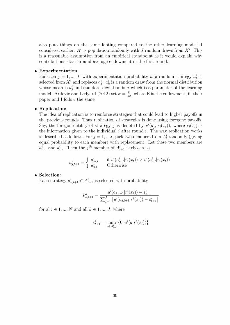
also puts things on the same footing compared to the other learning models Iconsidered earlier. Ai1 is population randomly with J random draws from X i. Thisis a reasonable assumption from an empirical standpoint as it would explain whycontributions start around average endowment in the first round.
• Experimentation:For each j = 1, ..., J , with experimentation probability ρ, a random strategy aik isselected from X i and replaces aij. a
ik is a random draw from the normal distribution
whose mean is aij and standard deviation is σ which is a parameter of the learning
model. Arifovic and Ledyard (2012) set σ = E10
, where E is the endowment, in theirpaper and I follow the same.
• Replication:The idea of replication is to reinforce strategies that could lead to higher payoffs inthe previous rounds. Thus replication of strategies is done using foregone payoffs.Say, the foregone utility of strategy j is denoted by vi(aijt|ri(xt)), where ri(xt) isthe information given to the individual i after round i. The way replication worksis described as follows. For j = 1, ...J , pick two members from Ait randomly (givingequal probability to each member) with replacement. Let these two members areaim,t and ain,t. Then the jth member of Ait+1 is chosen as:
aij,t+1 =
{aim,t if vi(aim,t|ri(xt)) > vi(ain,t|ri(xt))ain,t Otherwise
• Selection:Each strategy aik,t+1 ∈ Ait+1 is selected with probability
P ik,t+1 =
ui(ak,t+1|ri(xt))− εit+1∑Jj=1
[ui(aj,t+1|ri(xt))− εit+1
]for al i ∈ 1, ..., N and all k ∈ 1, ..., J , where
εit+1 = mina∈Ait+1
{0, ui(a|ri(xt))}
39