learning graphical models fundamental …learning graphical models fundamental limits and efficient...
TRANSCRIPT

LEARNING GRAPHICAL MODELS
FUNDAMENTAL LIMITS AND EFFICIENT ALGORITHMS
A DISSERTATION
SUBMITTED TO THE DEPARTMENT OF ELECTRICAL
ENGINEERING
AND THE COMMITTEE ON GRADUATE STUDIES
OF STANFORD UNIVERSITY
IN PARTIAL FULFILLMENT OF THE REQUIREMENTS
FOR THE DEGREE OF
DOCTOR OF PHILOSOPHY
Jose Bento
August 2012

Preface
Graphical models provide a flexible and yet powerful language to describe high di-
mensional probability distributions. Over the last 20 years, graphical models methods
have been successfully applied to a broad range of problems, from computer vision to
error correcting codes to computational biology, to name a few.
In a graphical model, the graph structure characterizes the conditional indepen-
dence properties of the underlying probability distributions. Roughly speaking, it
encodes key information about which variables influence each other. It allows us to
answer questions of the type: are variablesX and Y dependent because they ‘interact’
directly, or because they are both dependent on a third variable Z? In many applica-
tions, this information has utmost practical importance, and it is therefore crucial to
develop efficient algorithms to learn the graphical structure from data. This problem
is largely unsolved and for a long time several heuristics have been used without a
solid theoretical foundation in place.
In the first part of this work, we consider the problem of learning the structure
of Ising models (pairwise binary Markov random fields) from i.i.d. samples. While
several methods have been proposed to accomplish this task, their relative merits and
limitations remain somewhat obscure. By analyzing a number of concrete examples,
we show that low-complexity algorithms often fail when the Markov random field
develops long-range correlations. More precisely, this phenomenon appears to be
related to the Ising model phase transition (although it does not coincide with it).
An example of an important algorithm that exhibits this behavior is the ℓ1-
regularized logistic regression estimator introduced by Ravikumar et al. [94]. Raviku-
mar et al. [94] proved a set sufficient conditions under which this algorithm exactly
iv

learns Ising models, the most interesting being a so-called incoherence condition. In
this thesis we show that this incoherence condition is also necessary and analytically
establish whether it holds for several families of graphs. In particular, denoting by θ
the edge strength and by ∆ the maximum degree, we prove that regularized logistic
regression succeeds on any graph with ∆ ≤ 3/(10θ) and fails on most regular graphs
with ∆ ≥ 2/θ.
In the second part of this work, we address the important scenario in which data
is not composed of i.i.d. samples. We focus on the problem of learning the drift
coefficient of a p-dimensional stochastic differential equation (SDE) from a sample
path of length T . We assume that the drift is parametrized by a high-dimensional
vector, and study the support recovery problem in the case where p is allowed to grow
with T .
In particular, we describe a general lower bound on the sample-complexity T
by using a characterization of mutual information as a time integral of conditional
variance, due to Kadota, Zakai, and Ziv. For linear SDEs, the drift coefficient is
parametrized by a p-by-p matrix which describes which degrees of freedom interact
under the dynamics. In this case, we analyze an ℓ1-regularized least-squares estimator
and describe an upper bound on T that nearly matches the lower bound on specific
classes of sparse matrices.
We describe how this same algorithm can be used to learn non-linear SDEs and
in addition show by means of a numerical experiment why one should expect the
sample-complexity to be of the same order as that for linear SDEs.
v

vi

Acknowledgements
The work of this thesis was accomplished with support of many ‘hands’.
First, I am happy to thank God for His love. Without Him, my endeavors at
Stanford are worthless.
I would also like to thank Professor Andrea Montanari, my advisor, for his support,
encouragement, and guidance, and above all, for being an example of excellence in
research. The passion he has for his work has taught me first-hand a valuable lesson:
only those who love their work can excel.
I have also been privileged to be a part Andrea’s research group. During my stay
at Stanford I was able to interact with Sewoong, Satish, Moshen, Morteza, Raghu,
Adel, Yash and Yash. In particular, I was able to collaborate with Sewoong and
Morteza on two different projects.
In addition, I must thank my friends for their care and presence in my life through-
out these years. I would have to double the number of pages in this thesis if I even
attempted to summarize in a list the many benefits I have been granted through
them.
My family has also been indispensable in my success, for the indescribable joy
they bring me which fuels my life and gives me strength. In particular, I must thank
my mother, Nina, for always having many interesting stories to tell every Sunday
afternoon over Skype. I am also very happy for the support I have received from my
Godmother, Teresa. More visibly in the first years of my life but certainly still now,
at a distance.
I am also very thankful for all the help Professor Persi Diaconis gave me during
my time at Stanford and for the several interesting topics I have learned about from
vii

him. In particular, I am thankful for his availability to meet and help me overcome
mathematical hurdles and for kindly and habitually inquiring about the wellbeing of
my family.
I would also like to acknowledge Professor Iain Johnstone for his availability to
regularly discuss my research with him and also Professor Emmanuel Candes and
Professor Ramesh Johari for being part of my thesis defense and reading committee.
More over, I must thank Professor Tsachy Weissman for the availability to work with
me and guide me in my first year at Stanford.
Furthermore, I would like to thank Hewlett-Packard Labs and Technicolor Labs
in Palo Alto for providing me two wonderful summer internships. In particular, I
would like to thank Niranjan, Emon and Jerry from HP and Jinyun, Stratis, Nadia
and Jean from technicolor.
Finally, this work was partially supported by the Portuguese Doctoral FCT fel-
lowship SFRH / BD / 28924 / 2006.
viii

Contents
Preface iv
Acknowledgements vii
1 Introduction 1
1.1 Graphical models . . . . . . . . . . . . . . . . . . . . . . . . . . . . . 1
1.2 Structural learning in graphical models . . . . . . . . . . . . . . . . . 3
1.2.1 Sample-complexity and computational-complexity . . . . . . . 6
1.2.2 Dependencies in data . . . . . . . . . . . . . . . . . . . . . . . 8
1.3 Contributions . . . . . . . . . . . . . . . . . . . . . . . . . . . . . . . 10
1.4 Notation . . . . . . . . . . . . . . . . . . . . . . . . . . . . . . . . . . 15
2 Learning the Ising model 19
2.1 Introduction . . . . . . . . . . . . . . . . . . . . . . . . . . . . . . . . 20
2.1.1 A toy example . . . . . . . . . . . . . . . . . . . . . . . . . . . 23
2.2 Related work . . . . . . . . . . . . . . . . . . . . . . . . . . . . . . . 25
2.3 Main results . . . . . . . . . . . . . . . . . . . . . . . . . . . . . . . . 28
2.3.1 Simple thresholding algorithm . . . . . . . . . . . . . . . . . . 29
2.3.2 Conditional independence test . . . . . . . . . . . . . . . . . . 30
2.3.3 Regularized logistic regression . . . . . . . . . . . . . . . . . . 32
2.4 Important remark . . . . . . . . . . . . . . . . . . . . . . . . . . . . . 39
2.5 Numerical results . . . . . . . . . . . . . . . . . . . . . . . . . . . . . 39
2.6 Proofs for regularized logistic regression . . . . . . . . . . . . . . . . . 41
2.6.1 Notation and preliminary remarks . . . . . . . . . . . . . . . . 42
ix

2.6.2 Necessary conditions for the success of Rlr . . . . . . . . . . . 43
2.6.3 Specific graph ensembles . . . . . . . . . . . . . . . . . . . . . 44
2.6.4 Proof of Theorem 2.3.6 . . . . . . . . . . . . . . . . . . . . . . 46
2.6.5 Proof of Theorem 2.3.6: θ∆ ≤ 3/10 . . . . . . . . . . . . . . . 47
2.6.6 Proof of Theorem 2.3.6: θ∆ ≥ 2 . . . . . . . . . . . . . . . . . 47
2.6.7 Discussion . . . . . . . . . . . . . . . . . . . . . . . . . . . . . 49
2.7 Regularized logistic regression and graph families with additional struc-
ture . . . . . . . . . . . . . . . . . . . . . . . . . . . . . . . . . . . . 50
3 Learning stochastic differential equations 52
3.1 Introduction . . . . . . . . . . . . . . . . . . . . . . . . . . . . . . . . 54
3.2 Related work . . . . . . . . . . . . . . . . . . . . . . . . . . . . . . . 57
3.3 Main results . . . . . . . . . . . . . . . . . . . . . . . . . . . . . . . . 59
3.3.1 Notation . . . . . . . . . . . . . . . . . . . . . . . . . . . . . . 60
3.3.2 Regularized least squares . . . . . . . . . . . . . . . . . . . . . 60
3.3.3 Sample complexity for sparse linear SDE’s . . . . . . . . . . . 62
3.3.4 Learning the laplacian of graphs with bounded degree . . . . . 64
3.4 Important remark . . . . . . . . . . . . . . . . . . . . . . . . . . . . . 66
3.5 Important steps towards the proof of main results . . . . . . . . . . . 68
3.5.1 Discrete-time model . . . . . . . . . . . . . . . . . . . . . . . 68
3.5.2 General lower bound on time complexity . . . . . . . . . . . . 71
3.6 Numerical illustrations of the main theoretical results . . . . . . . . . 74
3.7 Extensions . . . . . . . . . . . . . . . . . . . . . . . . . . . . . . . . . 76
3.7.1 Learning Dense Linear SDE’s . . . . . . . . . . . . . . . . . . 76
3.7.2 Learning Non-Linear SDE’s . . . . . . . . . . . . . . . . . . . 77
3.8 Numerical illustration of some extensions . . . . . . . . . . . . . . . . 79
3.8.1 Mass-spring system . . . . . . . . . . . . . . . . . . . . . . . . 79
3.8.2 Biochemical pathway . . . . . . . . . . . . . . . . . . . . . . . 83
A Learning the Ising model 87
A.1 Simple Thresholding . . . . . . . . . . . . . . . . . . . . . . . . . . . 87
A.2 Incoherence is a necessary condition: Proof of Lemma 2.6.1 . . . . . . 89
x

A.3 Proof of Theorem 2.3.6: θ∆ ≤ 3/10 . . . . . . . . . . . . . . . . . . . 92
A.4 Graphs in Gdiam(p,∆): Proof of Lemma 2.6.3 . . . . . . . . . . . . . . 97
A.4.1 Graphs Gdiam(p) from the Section 2.6.3: Remark 2.3.1 and Re-
mark 2.6.1 . . . . . . . . . . . . . . . . . . . . . . . . . . . . . 104
A.5 Graphs in Grand(p,∆): Proof of Lemma 2.6.4 . . . . . . . . . . . . . . 108
B Learning stochastic differential equations 110
B.1 Upper bounds on sample complexity of the regularized least squares
algorithm . . . . . . . . . . . . . . . . . . . . . . . . . . . . . . . . . 110
B.2 Necessary condition for successful reconstruction of SDEs . . . . . . . 111
B.3 Concentration bounds . . . . . . . . . . . . . . . . . . . . . . . . . . 112
B.4 Proof of Theorem 3.5.1 . . . . . . . . . . . . . . . . . . . . . . . . . . 113
B.4.1 Details of proof of Theorem 3.5.1 . . . . . . . . . . . . . . . . 114
B.5 Proof of Theorem 3.3.1 . . . . . . . . . . . . . . . . . . . . . . . . . . 116
B.5.1 Auxiliary lemma for proof of Theorem 3.3.1 . . . . . . . . . . 117
B.6 Proofs for the lower bounds . . . . . . . . . . . . . . . . . . . . . . . 117
B.6.1 A general bound for linear SDE’s . . . . . . . . . . . . . . . . 118
B.6.2 Proof of Theorem 3.3.3 . . . . . . . . . . . . . . . . . . . . . . 119
Bibliography 124
xi

List of Tables
xii

List of Figures
1.1 Topology of G5: PG5(x1, ..., x5) = exp(x1x3 + x1x4 + x1x5 + x2x3 +
x2x4 + x2x5). . . . . . . . . . . . . . . . . . . . . . . . . . . . . . . . 6
1.2 From left to right: Graph for variant 1, variant 2 and variant 3. . . . 6
1.3 Learning uniformly generated random regular graphs of degree ∆ = 4
for the Ising model from samples using regularized logistic regression.
Red curve: success probability as a function of the edge-strength, i.e.
θij ∈ 0, θ . . . . . . . . . . . . . . . . . . . . . . . . . . . . . . . . . 12
1.4 Reconstruction of non-linear SDEs. Curves show minimum observation
time TRls required to achieve a probability of reconstruction of Psucc =
0.1, 0.5 and 0.9 versus the size of the network p. All non-linear SDEs
are associated to random regular graphs of degree 4 sampled uniformly
at random. The points in the plot are averages over different graphs
and different SDEs trajectories. . . . . . . . . . . . . . . . . . . . . . 13
2.1 Two families of graphs Gp and G′p whose distributions PGp,θ and PG′
p,θ′
merge as p gets large. . . . . . . . . . . . . . . . . . . . . . . . . . . 23
2.2 Learning random subgraphs of a 7 × 7 (p = 49) two-dimensional grid
from n = 4500 Ising models samples, using regularized logistic regres-
sion. Left: success probability as a function of the model parameter θ
and of the regularization parameter λ0 (darker corresponds to highest
probability). Right: the same data plotted for several choices of λ ver-
sus θ. The vertical line corresponds to the model critical temperature.
The thick line is an envelope of the curves obtained for different λ, and
should correspond to optimal regularization. . . . . . . . . . . . . . . 40
xiii

2.3 Learning uniformly random graphs of degree ∆ = 4 from Ising models
samples, using regularized logistic regression. Left: success probability
as a function of the number of samples n for several values of θ. Dotted:
θ = 0.10, 0.15, 0.20, 0.35, 0.40 (in all these cases θ < θthr(∆ = 4)).
Dashed: θ = 0.45, 0.50, 0.55, 0.60, 0.65 (θ > θthr(4), some of these
are indistinguishable from the axis). Right: the same data plotted for
several choices of λ versus θ as in Fig. 2.2, right panel. . . . . . . . . 41
2.4 Diamond graphs Gdiam(p). . . . . . . . . . . . . . . . . . . . . . . . . 44
3.1 (left) Probability of success vs. length of the observation interval nη.
(right) Sample complexity for 90% probability of success vs. p. . . . . 74
3.2 (right)Probability of success vs. length of the observation interval nη
for different values of η. (left) Probability of success vs. η for a fixed
length of the observation interval, (nη = 150) . The process is gener-
ated for a small value of η and sampled at different rates. . . . . . . . 76
3.3 Evolution of the horizontal component of the position of three masses
in a system with p = 36 masses interacting via elastic springs (cf.
Fig. 3.4 for the network structure). The time interval is T = 1000. All
the springs have rest length Dij = 1, the damping coefficient is γ = 2,
cf. Eq. (3.8.1), and the noise variance is σ2 = 0.25. . . . . . . . . . . 80
3.4 From left to right and top to bottom: structures reconstructed using
Rlr with observation time T = 500, 1500, 2500, 3500 and 4500. For
T = 4500 exact reconstruction is achieved. . . . . . . . . . . . . . . . 81
3.5 (left) Probability of success versus length of observation time window,
T , for different network sizes (p = 8, 16, 32, 64 and 128). (right) Min-
imum number of samples required to achieve a probability of recon-
struction of Psucc = 0.1, 0.5 and 0.9 versus the size of the network p.
All networks where generated from random regular graphs of degree 4
sampled uniformly at random. The dynamics’ parameters were set to
σ = 0.5 and γ = 0.1 . . . . . . . . . . . . . . . . . . . . . . . . . . . . 83
xiv

3.6 (left) True positive rate (right) false positive rate vs. λ for the duration
of observation T = 1200. . . . . . . . . . . . . . . . . . . . . . . . . . 85
3.7 (left) ROC curves for different values of T . (right) Area under the
ROC curve vs. T . . . . . . . . . . . . . . . . . . . . . . . . . . . . . . 86
3.8 (left) NRMSE vs. λ; T = 1200. (right) NRMSE vs. T for the optimum
value of λ. . . . . . . . . . . . . . . . . . . . . . . . . . . . . . . . . . 86
A.1 For this family of graphs of increasing maximum degree ∆ Rlr(λ) will
fail for any λ > 0 if θ ≥ 2/∆. . . . . . . . . . . . . . . . . . . . . . . 104
A.2 Solution curves of Rlr(λ) as a function of λ for different values of θ
and p = 5. Along each curve, λ increases from right to left. Plot
points separated by δλ = 0.05 are included to show the speed of the
parameterization with λ. For λ → ∞ all curves tend to the point
(0, 0). For λ = 0, θ13 = θ. Remark: Curves like the one for θ = 0.55
are identically zero above a certain value of λ. . . . . . . . . . . . . . 105
A.3 F (β) for p = 6. Red θ = 0.1, 0.2, 0.3. Blue θ = 0.4, 0.5, 0.6. . . . . . . 107
xv

Chapter 1
Introduction
In a nutshell, in this thesis we look at stochastic models parametrized by an unknown
graph - graphical models - and address the following question:
Question. Is it possible to recover the graph from data?
1.1 Graphical models
Graphical models are a language to compactly describe large joint probability dis-
tributions using a set of ‘local’ relationships among neighboring variables in a graph
[33, 74, 77, 71]. The ‘local’ relationships are described by functions involving neigh-
boring variables in this graph that are related to conditional probability distributions
over these variables. The product of these functions equals the joint distribution. Let
us be precise. Given a set of variables x = x1, ..., xp that take a value in −1,+1,we can start from a local model of how likely it is that any two variables assume the
same value, −1 or +1, and obtain a joint model for the probability that x takes a
certain value in −1, 1p. For example, the local model can describe two scenarios:
any two variables xi, xj , are either ‘connected’ with strength θij 6= 0 or ‘disconnected’,
θij = 0. If two variables xi and xj are connected, we include a factor eθijxixj in the
joint probability distribution, and if disconnected, we include a factor 1. Given a
1

CHAPTER 1. INTRODUCTION 2
weighted graph G = (V,E) with vertex set V and edge set E, (V = [p] ≡ 1, ..., p,E = (i, j) : θi,j 6= 0) and assuming every two variables obey the same local model
described above, the joint probability distribution of a configuration of x is given by
PG(x) =1
ZG
∏
(i,j)∈Eeθijxixj , (1.1.1)
where ZG is a normalization constant. The above model is an example of a graphical
model and is known as the Ising model.
Graphical models find many applications. For example, the above model has been
used to understand the evolution of opinions in closed communities [105]. There, G
describes a set of acquaintanceships among individuals in a community. Individuals
‘connected’ by a positive bond θij > 0 are more likely to assume the same opinion,
−1 or −1, on a given matter. Ising models are also used in computer vision, where
G describes a set of pixels in an image to be de-noised [112, 79] or pixels in a pair of
stereoscopic images to be used for depth perception [106]. Computational biologists
use other graphical models where G represents a network of interacting genes that
regulate cell activities [48, 47, 73, 58] or the amino-acids in a protein that interact
with themselves and other bio-entities to determine their shape and function [59,
111]. In digital communications, codes are constructed by designing graphs that
represent parity-check constraints on the bits of codewords and decoding is done
by computations on these graphs [50, 28, 80, 95]. In computational neurobiology,
to understand the functioning of the brain, scientists use graphical models where G
represents a map of neural connections in the brain [34, 64, 22, 113]. Graphical models
also find applications in meteorology [23].
These applications pose different challenges related to graphical models. Four
of the main problems are: representation, sampling, inference and learning. See
[69, 18, 75] for a review on the several research questions associated with graphical
models. Representation concerns choosing the right model for the application at
hand. Different kinds of graphical models include Markov random fields (based on
undirected graphs) , Bayesian networks (based on directed graphs) and factor graphs.
In this thesis we focus only on pair-wise Markov random fields and on stochastic

CHAPTER 1. INTRODUCTION 3
differential equations. Sampling refers to the problem of generating samples from
the model’s probability distribution. Inference is about using the model to answer
probabilistic queries - for example, computing marginal probabilities or inferring the
value of unobserved variables. The problem of learning focuses on recovering the
model from data, as when we estimate the values of the parameters θij in model
(1.1.1). This is important because often we start with no details about the model.
In many applications the interest is specifically in recovering the support of these
parameters. For the Ising model, this corresponds to determining which coefficients
θij are non-zero. Herein lies the focus of this thesis, which can be described as an
investigation into how the graph G can be learned from data. Concerning this last
problem, we note that several variants can be conceived which we do not address.
For example, how do we learn the graph from partially hidden data? Regarding the
questions addressed in this thesis, these hidden data can come, for example, from
unobserved nodes in the graph [97, 46, 7]. This is relevant in evolutionary biology as
a way to model the change in gene-data along the evolution-tree of a group of species
[84, 99]. Hidden data can also arise from points in the trajectory of a stochastic
differential equation which are not sampled [31, 91, 5]. This is the case in many
applications where sampled data come at a very low frequency compared with the
dominant frequency modes in the system.
1.2 Structural learning in graphical models
One of the most important properties of graphical models is that the underlying graph
describes a set of conditional independence relations among variables. This relation
is made precise by the Hammersley-Clifford theorem [57, 17],
Theorem 1.2.1. Let G = (V = [p], E) be an undirected graph and CG the set of all
maximal cliques in G. A probability distribution P(x1, ..., xp) > 0 factorizes according
to G
P(x) =1
Z
∏
c∈CG
Φc(xc) (1.2.1)

CHAPTER 1. INTRODUCTION 4
if and only if,
P(xi|xG\i) = P(xi|x∂i), for all i ∈ V . (1.2.2)
In the expressions above, Z is a normalization constant, for any set c ⊆ V , xc = xj :
j ∈ c and ∂i = j ∈ V : (i, j) ∈ E.
In fact, when the above equivalence holds, all the following three conditional
independence relations hold:
• A variable is conditionally independent of all other variables given its neighbors;
• Any two non-connected variables ((i, j) /∈ E) are conditionally independent
given all other variables;
• Any two subsets of variables, A, B, are conditionally independent given a sep-
arating subset C, where every path from A to B passes through C.
For the Ising model (1.1.1) over a graph G, since PG(x) > 0 and PG(x) factorizes
according to G, all conditional independence property above hold.
Understanding the dependencies among a set of variables is of great importance
for many applications and is almost always a prerequisite for further modeling efforts.
In particular, it allows us to solve the confounding variable problem: Given three
different variables - X , Y and Z - does X affect Z directly, or only through Y ?
For concrete examples, these conditional dependencies can have interesting in-
terpretations. Consider the Ising model where the vertices represent people holding
one of two opinions, −1 or +1, on a certain matter. The edges, all with equal posi-
tive weight, represent influence links. Two people who are connected have a higher
chance of holding the same opinion. Now let A, B and C be groups of individuals
(A,B,C ⊂ V ) such that, if members of group C were to disappear, there would be
no connection between group A and B. Then, conditioned on the opinion of all the
members of group C being fixed, the members of group A and B cannot influence
each other.
The question formulated in the beginning which motivates the work in this thesis
amounts to recovering this set of dependencies. For the Ising model (1.1.1), a partic-
ular instance of this problem can be written as

CHAPTER 1. INTRODUCTION 5
Question. Is it possible to recover G given n independent identically distributed
(i.i.d.) samples from PG(x)?
This problem appears in the literature under the name of structural learning of
graphical models (e.g. [25, 42, 47, 18, 3, 29, 2]). Learning G is equivalent to learning
which coefficients of θ ≡ θij are non-zero, i.e. learning the support of θ, i.e. supp(θ).The problem of learning G is a special case of the general estimation problem [78,
41]. In the general estimation problem, given samples x(ℓ) from a parametrized
probability distribution Pθ(x), the objective is to compute an estimate θ for θ under
an appropriate loss function. Structural learning is estimation under the loss function
C(θ, θ) = I(supp(θ) 6= supp(θ)). (1.2.3)
When related to graphical models, the estimation problem often goes under the sim-
pler name of learning graphical models, to distinguish it from structural learning, and
often the cost function assumed is the Euclidean norm of the difference between true
and estimated parameters.
This difference in norms does change our problem from the usual estimation prob-
lem in a fundamental way. In particular, there is a difference between knowing
whether a given coefficient is approximately zero (approximating θ) and knowing
whether a coefficient is exactly zero, i.e., estimating G. Recovering G = (V,E) from
data allows us, for example, to find a sets A,B,C ∈ V such that, conditioned on the
variables in C, the variables in A and B are independent. However, from a set real
parameters θij, some of smaller magnitude than others, it is unclear how we should
select such sets.
In addition, in parameter learning for graphical models we know from the start
the structure of the solution, i.e., which coefficients are non-zero [86]; while in this
thesis, finding them is our objective.

CHAPTER 1. INTRODUCTION 6
2
3
5
4
1
Figure 1.1: Topology of G5: PG5(x1, ..., x5) = exp(x1x3 + x1x4+ x1x5+ x2x3 +x2x4 +x2x5).
2
3
5
4
1
θ = 0.1θ = 1θ = 1
Figure 1.2: From left to right: Graph for variant 1, variant 2 and variant 3.
1.2.1 Sample-complexity and computational-complexity
To illustrate some of the challenges of structural learning we now focus on a particular
instance of the model (1.1.1). There is a set of five nodes connected by two kinds
of links: any two nodes are either connected, θij = 1, or disconnected, θij = 0. In
this model, the graph, G5, has the topology shown in Figure 1.1. Since (1.1.1) is an
exponential family, given n i.i.d samples from PG5(x), the set of empirical covariances
Cij = (1/n)∑n
ℓ=1 x(ℓ)i x
(ℓ)j is a sufficient statistic to recover G5 [78]. As a first attempt
to recover G5, we compute all Cij and use the following threshold rule: If Cij > τ ,
we conclude that (i, j) ∈ E; otherwise, we do not. However, even in the favorable
case where n = ∞, one can see that such an attempt would not work. For n = ∞,
C12 ≈ 0.963 > C13 ≈ 0.946 and the threshold rule says either that both edges (1, 2)
and (1, 3) are in E or that E excludes both. In either case, we do not recover G5
correctly. Consider now the following three variants of the network of Figure 1.1.
These variants are illustrated in Figure 1.2.
• Variant 1 (topological change): Start fromG5 and remove edges (1, 5) and (5, 2).

CHAPTER 1. INTRODUCTION 7
• Variant 2 (topological change): Start from G5 and add edges (3, 4) and (4, 5).
• Variant 3 (edge-strength change): Start from G5 and reduce the edge-weights
from θij ∈ 0, 1 to θij ∈ 0, 0.1.
Surprisingly, for these three variants, at least when n = ∞, we can recover the
underlying graph from this simple threshold rule. When n = ∞, successful recon-
struction by thresholding for variant 1 and variant 3 is equivalent, by symmetry,
to C13 > maxC34, C12. Namely, for variant 1, C13 ≈ 0.100, C34 ≈ 0.020 and
C12 ≈ 0.020 and for variant 3, C13 ≈ 0.102, C34 ≈ 0.020 and C12 ≈ 0.030. For variant
2, when n = ∞, the success is equivalent, by symmetry, to minC13, C34 > C12.
Correspondingly, C13 ≈ 0.989, C34 ≈ 0.993 and C12 ≈ 0.987.
The above examples show that while some graphs are recoverable by fairly simple
algorithms, other similar graphs might be harder to learn. Because of this, most
algorithms proposed in the literature are only guaranteed to work under specific
restrictions on the class of graphs [3, 21, 94, 1]. In addition, the class of graphs that in
principle it might be possible to learn does not seem to have a simple characterization.
Making a graph denser (by adding edges) or sparser (by removing edges) sometimes
makes a particular algorithm succeed and other times fail. Furthermore, not only the
topology, but also the edges-weights, must be taken into account.
There are other nuances: among graphs that are recoverable with simple algo-
rithms there are also differences. The gap between the correlation of connected and
disconnected nodes is greater than 0.07 in variants 1 and 3 but in variant 2 is smaller
than 0.002. Using the thresholding algorithm to recover variant 1 and 3 therefore
requires using less samples (smaller n) than to recover variant 2. The notions of
sample-complexity and computational-complexity are introduced to quantify these dif-
ferences. Given an algorithm Alg that receives as input n samples from PG(x) and
outputs a graph G, the sample-complexity is defined by
NAlg(G) ≡ minn0 ∈ N : PG,nG = G ≥ 1− δ for all n ≥ n0
(1.2.4)
where PG,n denotes probability with respect to n i.i.d. samples with distribution PG,n.
The computational complexity χAlg(G) is the running time of Alg on an input of size

CHAPTER 1. INTRODUCTION 8
n = NAlg(G). The question generally addressed in this thesis can be expressed using
these two quantities:
Question. What are the values of NAlg(G) and χAlg(G) for different families of graphs
and algorithms?
We are particularly interested in understanding how NAlg(G) and χAlg(G) scale
with the size p of G (recall |V | = p). This is different from the classical learning
setting where n ≫ p. The recent explosion of data collection and storage puts many
applications in the regime n ≫ p, but for many problems, the number of variables
involved is unavoidably greater than the amount of data. To attack these problems,
we wish to find algorithms for which both the sample-complexity and computational-
complexity scale slowly with p. How slowly can these quantities scale? As a reference
for computational-complexity, notice that the thresholding algorithm used above,
one of the simplest algorithms we can think of, has a running time that scales likes
O(np2) 1. As a reference for sample-complexity, consider the minimum number of i.i.d.
samples needed to identify a graph among the class of graphs of degree bounded by
∆. Each sample on a graph with p nodes gives p bits of information and the number
of graphs of degree bounded by ∆ on p nodes is O((
p∆
)p)hence pn = O
(p log
(p∆
))
or n = O(∆ log p).
1.2.2 Dependencies in data
In our discussion of learning the Ising model, we have assumed data are composed of
i.i.d. samples from the constructed probability distribution. However, in many ap-
plications data are gathered in time and samples are not independent but correlated.
This reality brings additional questions to the problem of structural learning. This
thesis addresses some of them. Going back to the Ising model, a simple dynamical
model can be obtained by constructing a Gibbs sampler for (1.1.1) [51, 24]: If at time
1There are p2 empirical correlations to be computed each taking O(n) time steps to be computed.
CHAPTER 1. INTRODUCTION 9
t the configuration is x(t), we form the configuration at time t+1, x(t+1), by choos-
ing a node i uniformly at random from V and ‘flipping’ its value with probability
min1, exp(−2xi
∑j θijxj(t)). This dynamical model is a reversible Markov chain
with unique stationary measure equal to the model (1.1.1). If we have an algorithm
Alg for learning G that provably works when the input values are i.i.d. samples, one
can now think of circumventing the correlation among samples by inputting to Alg the
subsequence x(m), x(2m), ..., x(m⌊n/m⌋). If m is sufficiently large, x(im is close to
set of i.i.d. samples and we expect that Alg(x(im) = G with high probability. But
is this the best we can do? Discarding information increases the sample-complexity,
hence the general question:
Question. How does NAlg(G) change when learning is done from correlated samples?
The answer to this question depends on the stochastic process generating the
correlated samples. In this thesis we study an extreme case of structural learning
with correlations in data: dynamical processes in continuous time. In particular,
our focus is on stochastic differential equations parametrized by graphs. A good
introduction to SDEs is found in [88]. At this point it is easier to have in mind a
concrete example. One of the simplest SDE models represents the fluctuation of the
value of a node i, xi(t), as a linear combination of the fluctuation of the value of
neighboring nodes in a graph G. More precisely, given a weighted graph G = (V,E)
with V = [p], E = (i, j) : θij 6= 0, we define
dxi(t) =∑
j
θijxj(t)dt+ dbi(t), (1.2.5)
where b(t) is a p-dimensional standard Brownian motion. The above equation is a
linear stochastic differential equation and is also a graphical model: the support of the
matrix Θ = θij defines the adjacency matrix of the graph G. Given the evolution
of these values, x(t), in a time window of length T , the particular question we are
interested in is:

CHAPTER 1. INTRODUCTION 10
Question. It is possible to recover G from x(t)Tt=0?
Unlike in the previous questions, no matter how small T is, we now have at our
disposal an infinite number of samples, since the trajectories are continuous. Perhaps,
then, we only need an arbitrarily small time window to recover G? But samples
obtained close it time exhibit a strong correlation, and it is reasonable to expect that
larger graphs (bigger p) require longer observation time windows to be recovered.
Hence, perhaps T scales like O(p)? Given an algorithm Alg that receives as input
a trajectory x(t)Tt=0 and outputs a graph G, we introduce the following modified
notion of sample-complexity for SDEs,
TAlg(G) = infT0 ∈ R
+ : PG,TG = G ≥ 1− δ for all T ≥ T0
, (1.2.6)
where PG,T denotes probability with respect to a trajectory of length T . The problem
of structural learning for SDEs that we address in this thesis is now precisely defined:
Question. What are the values of TAlg(G) and χAlg(G) for different families of SDEs
and algorithms?
Here also, our focus is on the regime of ‘large-systems and few data’, or p ≫ T .
The more classical problem of estimating the values of Θ [76, 12], known as system-
identification or drift-estimation, is again related to the problem we address, under
a suitable choice of error function. However, past work has not focused on support
recovery.
1.3 Contributions
Apart from the Introduction and Conclusion, this thesis is divided into two main
chapters. Chapter 2 concerns learning the structure the Ising model. This model

CHAPTER 1. INTRODUCTION 11
is interesting because of its applications (e.g., in computer vision and biology) and
its simplicity: it is the simplest model on binary variables for which the set of all
pair-wise correlations forms a sufficient statistic. While several methods have been
proposed to recover G in the Ising model, their relative merits and limitations remain
somewhat obscure. We analyze three different reconstruction algorithms and relate
their success or failure to a single criterion [68]:
Contribution. When the Ising model develops long-range correlations these algo-
rithms fail to reconstruct G in polynomial time (χG = O(poly(p))).
More concretely, for three polynomial time algorithms, and for Ising models of
bounded degree ∆ with homogeneous edge-weights of strength θ, there are constants C
and C ′ such if ∆θ < C then NAlg(G) = O(log p) and if if ∆θ > C ′ then NAlg(G) = ∞.
Among the three algorithms studied, most of our focus was on the regularized lo-
gistic regression algorithm introduced by by Ravikumar et al. [94]. [94]. [94] proved
a set sufficient conditions under which this algorithm exactly learns Ising models,
the most interesting being a so-called incoherence condition. In Chapter 2, we show
that this incoherence condition is also necessary and analytically establish whether it
holds or not for several families of graphs. In particular, for this algorithm we obtain
a sharp characterization of the two unspecified constants above [16].
Contribution. Regularized logistic regression succeeds on any graph with ∆θ ≤ 3/10
and fails on most regular graphs with ∆θ ≥ 2.
These results are well illustrated by Figure 1.3. The plot illustrates the probability
of successful reconstruction of regular graphs of degree 4 using regularized logistic
regression as a function of θ when θij ∈ 0, θ. When θ > θc, it is no longer possible
to learn G. θc is the critical temperature of the lattice and, for regular graphs, scales
like 1/∆, just as predicted by our sharp bounds.

CHAPTER 1. INTRODUCTION 12
0
0.2
0.4
0.6
0.8
1
1.2
0 0.1 0.2 0.3 0.4 0.5 0.6 0.7 0.8θ
θc
Psucc
Figure 1.3: Learning uniformly generated random regular graphs of degree ∆ = 4 forthe Ising model from samples using regularized logistic regression. Red curve: successprobability as a function of the edge-strength, i.e. θij ∈ 0, θ .
Chapter 3 treats of learning systems of SDEs. There we prove a general lower
bound on the sample-complexity TAlg(G) by using a characterization of mutual in-
formation as time a integral of conditional variance, due to Kadota, Zakai, and Ziv.
For linear SDEs, we analyze an ℓ1-regularized least-squares algorithm, Rls, and prove
an upper bound on TRls(G) which nearly matches the general lower bound [14, 15, 13].
Contribution. For linear and stable SDEs, if G has maximum degree bounded by
∆ then TRls(G) = O(log p) and any algorithm Alg with probability of success greater
than 1/2 on this class of graphs has TAlg(G) = Ω(log p). If G is a dense graph then
TRls(G) = O(p) and any algorithm Alg with probability of success greater than 1/2 on
this class of graphs has TAlg(G) = Ω(p). In both cases, the upper bound is achieved by
Rls and χRls = O(poly(p)).
Although our theoretical results only apply for linear SDEs, the algorithm pro-
posed has much greater applicability. In particular, it seems to be able to learn
even non-linear SDEs. This result is summarized in Figure 1.4 for the case of sparse
graphs. As the figure shows, even for non-linear SDEs, the sample-complexity in

CHAPTER 1. INTRODUCTION 13
2^3 2^4 2^5 2^6 2^7
0
25
50
75
100
125
150
175
200
225
250
Psucc
= 0.1
Psucc
= 0.5
Psucc
= 0.9
p
TRls
Figure 1.4: Reconstruction of non-linear SDEs. Curves show minimum observationtime TRls required to achieve a probability of reconstruction of Psucc = 0.1, 0.5 and0.9 versus the size of the network p. All non-linear SDEs are associated to randomregular graphs of degree 4 sampled uniformly at random. The points in the plot areaverages over different graphs and different SDEs trajectories.

CHAPTER 1. INTRODUCTION 14
reconstructing sparse graphs scales like O(log p).

CHAPTER 1. INTRODUCTION 15
1.4 Notation
Throughout this thesis, notation is introduced as needed. However, for convenience,
we summarize here the main conventions used, unless stated otherwise.
N Set of natural numbers 1, 2, ...;Z Set of integer numbers ...,−2,−1, 0, 1, 2, ...;R Set of real numbers;
[i] Subset of integer numbers 1, 2, ..., i;supp(.) Support of a vector/matrix, i.e., the set of indices
with non-zero values;
sign(.) Signed support of a vector/matrix, i.e., the set of
indices with positive values and the set of indices
with negative values;
AC ⊆ B If A is a subset of B then AC is the complement
of A in B. It will be clear from the context what B is;1 All-ones vector;I Identity matrix;
v∗,M∗ Transpose of vector v or matrix M ;
‖.‖0, ‖.‖1, ‖.‖2, ‖.‖F , ‖.‖∞ 0-norm, 1-norm, euclidean norm, Frobenius norm,
infinity norm;
Λmax(M),Λmin(M) Maximum and minimum eigenvalue of matrix M ;
σmax(M), σmin(M) Maximum and minimum singular of matrix M ;
〈v, w〉 Inner product of vector v and w (dot-product in
euclidean space);
Tr(A) Trace of matrix A;
|A| Determinant of matrix A;
vA,MAB If A and B are subset of indices then vA is the vector
formed by the entries of v whose indices are in A
and MAB is matrix formed by the entries of M whose

CHAPTER 1. INTRODUCTION 16
row indices are in A and column indices are in B;
∇f Gradient of function f ;
Hess(f) Hessian of function f ;
J(f) Jacobian of function f ;
θ, θ,Θ Parameters describing probability distributions;
θ0,Θ0 Unknown value of parameters whose support
estimation is this thesis’ main focus;
θ, Θ Estimate of parameters θ0 and Θ0;
S, S0 support of θ and θ0;
S Estimate of S0;
z0 Sub-gradient of ‖θ‖1 evaluated at θ0;
z Sub-gradient of ‖θ‖1 evaluated at θ;
P(.) Probability distribution parameterized by (.);
‘i.i.d.’ Independent and identically distributed;
P(.),n Probability distribution of n i.i.d samples from P(.);
E(.) Expected value over the probability distribution P(.);
E(.),n Expected value over the probability
distribution P(.),n;
Var(.) Variance with respect to the probability
distribution P(.);
Psucc Probability of successful reconstruction of a graph
G = (V,E) (successful reconstruction means full exact
recovery of E);
b(t) Standard Brownian motion;
x,X Sample from P(.) (deterministic and random variables
respectively);
x(ℓ), X(ℓ), x(t), X(t) Samples from P(.) indexed by integer number ℓ and
indexed by real number t;
Xn0 , X
T0 Samples x(ℓ)nℓ=0 and x(t)Tt=0;
G = (V,E) Graph with edge set E and vertex set V ;
∆G Laplacian of graph G;

CHAPTER 1. INTRODUCTION 17
∂r ⊆ V Neighborhood of node r ∈ V of
a graph G;
deg(r) Degree of node r, i.e., number of neighbors of node
r ∈ V of a graph G;
∆ Maximum degree across all nodes in a graph G;
p Number of nodes in graph G, the dimension of θ or
the ‘width’ of a matrix Θ ∈ Rm×p;
Gone Family of ‘one-edge’ graphs introduced in
Section 2.6.3;
Gdiam Family of ‘diamond’ graphs introduced in
Section 2.6.3;
Grand Family of regular graphs introduced in Section 2.6.3;
n Number of samples being used for reconstruction;
T Length of trajectory being used for reconstruction;
Alg General reconstruction algorithm;
Thr Thresholding algorithm of Section 2.3.1;
Ind Conditional independence algorithm of Section 2.3.2;
Rlr Regularized logistic regression algorithm of
Section 2.3.3;
Rls Regularized least squares algorithm of Section 3.3.2;
λ Regularization parameter;
NAlg(G) Minimum number of samples that Alg requires to
reconstruct the graph G of a specific graphical model;
NAlg(G, θ) Minimum number of samples that Alg requires to
reconstruct G for an homogeneous-edge-strength Ising
model of edge-strength θ;
NAlg(p,∆, θ) Minimum number of samples required
by Alg to reconstruct any graph G with p
nodes and maximum degree ∆ for an
homogeneous-edge-strength Ising model of
edge-strength θ;
CHAPTER 1. INTRODUCTION 18
TAlg(G) Minimum observation time that Alg requires to
reconstruct the graph G of a SDE parametrized by G;
TAlg(Θ) Minimum observation time that Alg requires to
reconstruct the signed support of Θ of a
SDE parametrized by Θ;
TAlg(A) Minimum observation time required by Alg to
reconstruct a family of SDEs denoted by A;
χAlg(G) Number of computation steps that Alg requires to
reconstruct the graph G of a specific graphical model
when run on NAlg(G) samples;
χAlg(G, θ) Number of computation steps that Alg requires to
reconstruct G for an homogeneous-edge-strength Ising
model of edge-strength θ when run on NAlg(G, θ)
samples;
χAlg(p,∆, θ) Number of computation steps required to
reconstruct any graph G with p nodes and maximum
degree ∆ for an homogeneous-edge-strength Ising
model of edge-strength θ when run on NAlg(p,∆, θ)
samples;
SDE Stochastic differential equation;
NRMSE Normalized root mean squared error
(‖Θ0 − Θ‖2/‖Θ0‖2);
Chapter 2
Learning the Ising model
This chapter is devoted to studying the sample-complexity and computational-complexity
of learning the Ising model for a number of reconstruction algorithms and graph mod-
els. The Ising model has already appeared in Chapter 1 in equation (1.1.1), but is
introduced in more detail in Section 2.1. In particular, we consider homogeneous
edge-strengths, i.e. θij ∈ 0, θ, and graphs of maximum degree bounded by ∆.
Results of this analysis are presented in Section 2.3 for three algorithms. A sim-
ple thresholding algorithm is discussed in Section 2.3.1. In Section 2.3.2, we look
at the conditional independence test method of [21]. Finally, in Section 2.3.3, we
study the penalized pseudo-likelihood method of [94]. In Section 2.5, we validate our
analysis through numerical simulations, and Section 2.6 contains the proofs of these
conclusions, with some technical details deferred to the appendices.
Our analysis unveils a general pattern: when the model develops strong correla-
tions, several low-complexity algorithms fail, or require a large number of samples.
What does ‘strong correlations’ mean? Correlations arise from a trade-off between
the degree (which we characterize here via the maximum degree ∆), and the interac-
tion strength θ. It can be ascribed to a few strong connections (large θ) or to a large
number of weak connections (large ∆). Is there any meaningful way to compare and
combine these quantities (θ and ∆)? An answer is suggested by the theory of Gibbs
measures which predicts a dramatic change of behavior of the Ising model when θ
crosses the so-called ‘uniqueness threshold’ θuniq(∆) = atanh(1/(∆ − 1)) [52]. For
19
CHAPTER 2. LEARNING THE ISING MODEL 20
θ < θuniq(∆), Gibbs sampling mixes rapidly and far-apart variables in G are roughly
independent [85]. Conversly, for any θ > θuniq(∆), there exist graph families on which
Gibbs sampling is slow, and far-apart variables are strongly dependent [53]. While
polynomial sampling algorithms exist for all θ > 0 [70], for θ < 0, in the regime
|θ| > θuniq(∆) sampling is #-P hard [101]. Related to the uniqueness threshold is the
critical temperature, which is graph-dependent, with typically θcrit ≤ const./∆.
In this chapter we see that the theory of Gibbs measure is indeed a relevant
way of comparing interaction strength and graph degree for the problem of structural
learning. All the algorithms we analyzed provably fail for θ ≫ const./∆, for a number
of ‘natural’ graph families. This chapter raises several fascinating questions, the
most important being the construction of structural learning algorithms with provable
performance guarantees in the strongly dependent regime θcrit ≫ const./∆. The
question as to whether such an algorithm exists is left open by the present thesis (but
see Section 2.2 for an overview of earlier work).
Let us finally emphasize that we do not think that any of the specific families
of graphs studied in the present thesis is intrinsically ‘hard’ to learn. For instance,
we show in Section 2.3.3 that the regularized logistic regression method of [94] fails
on random regular graphs, while it is easy to learn such graphs using the simple
thresholding algorithm of Section 2.3.1. The specific families were indeed chosen
mostly because they are analytically tractable.
The work in this chapter is based on joint work with Montanari [68, 16].
2.1 Introduction
Given an undirected graph G = (V = [p], E), and a positive parameter θ > 0, the
ferromagnetic Ising model on G is the pair-wise Markov random field
PG,θ(x) =1
ZG,θ
∏
(i,j)∈Eeθxixj (2.1.1)
over binary variables x = (x1, x2, . . . , xp), xi ∈ +1,−1. Apart from being one of the
best-studied models in statistical mechanics [66, 56], the Ising model is a prototypical

CHAPTER 2. LEARNING THE ISING MODEL 21
undirected graphical model. Since the seminal work of Hopfield [65] and Hinton
and Sejnowski [62], it has found application in numerous areas of machine learning,
computer vision, clustering and spatial statistics. The obvious generalization of the
distribution (2.1.1) to edge-dependent parameters θij , (i, j) ∈ E is of central interest
in such applications
Pθ(x) =1
Zθ
∏
(i,j)∈E(Kp)
eθijxixj , (2.1.2)
where E(Kp) ≡ (i, j) : i, j ∈ V is the edge set of the complete graph and
θ = θij(i,j)∈E(Kp) is a vector of real parameters. The support of the parameter
θ specifies a graph. In fact, model (2.1.1) corresponds to θij = 0, ∀(i, j) /∈ E and
θij = θ, ∀(i, j) ∈ E. Let us stress that we follow the statistical mechanics convention
of calling (2.1.1) an Ising model even if the graph G is not a grid.
In this section we focus on the following structural learning problem:
Given n i.i.d. samples x(1), x(2),. . . , x(n) ∈ +1,−1p with distribution
PG,θ( · ), reconstruct the graph G.
For the sake of simplicity, we assume the parameter θ is known, and that G has no
double edges (it is a ‘simple’ graph). It follows from the general theory of exponential
families that, for any θ ∈ (0,∞), the model (2.1.1) is identifiable [78]. In particular,
the structural learning problem is solvable with unbounded sample complexity and
computational resources. The question we address is: for which classes of graphs
and values of the parameter θ is the problem solvable under realistic complexity
constraints? More precisely, given a graph G, an algorithm Alg that outputs an
estimate G = Alg(x(1), x(2), . . . , x(n)), a value θ of the model parameter, and a small
δ > 0, the sample complexity is defined as
NAlg(G, θ) ≡ minn0 ∈ N : PG,θ,nG = G ≥ 1− δ for all n ≥ n0
, (2.1.3)
where PG,θ,n denotes probability with respect to n i.i.d. samples with distribution
PG,θ. Further, we let χAlg(G, θ) denote the number of operations of the algorithm Alg,
when applied to NAlg(G, θ) samples. The general problem is therefore to characterize
CHAPTER 2. LEARNING THE ISING MODEL 22
the functions NAlg(G, θ) and χAlg(G, θ), and to design algorithms that minimize the
complexity.
Let us emphasize that these are not the only possible definitions of sample and
computational complexity. Alternative definitions are obtained by requiring that the
reconstructed structure Alg(x(1), . . . , x(n)) is only partially correct. However, for the
algorithms considered in this paper, such definitions should not result in qualitatively
different behavior1
General upper and lower bounds on the sample complexity NAlg(G, θ) were proved
by Santhanam and Wainwright [108, 98], without however taking into account com-
putational complexity. At the other end of the spectrum, several low complexity
algorithms have been developed in the last few years (see Section 2.2 for a brief
overview). Yet the resulting sample complexity bounds only hold under specific as-
sumptions on the underlying model (i.e., on the pair (G, θ)). A general understanding
of the trade-offs between sample complexity and computational complexity is largely
lacking.
This paper is devoted to the study of the tradeoff between sample complexity
and computational complexity for some specific structural learning algorithms, when
applied to the Ising model. An important challenge consists in the fact that the
model (2.1.1) induces subtle correlations between the binary variables (x1, . . . , xp).
The objective of a structural learning algorithm is to disentangle pairs xi, xj that are
conditionally independent given the other variables (and hence are not connected by
an edge) from those that are instead conditionally dependent (and hence connected
by an edge in G). This becomes particularly difficult when θ becomes large and hence
pairs xi, xj that are not connected by an edge in G become strongly dependent. The
next section sets the stage for our work by discussing a simple and concrete illustration
of this phenomenon.

CHAPTER 2. LEARNING THE ISING MODEL 23
Figure 2.1: Two families of graphs Gp and G′p whose distributions PGp,θ and PG′
p,θ′
merge as p gets large.
2.1.1 A toy example
As a toy illustration2 of the challenges of structural learning, we will study the two
families of graphs in Figure 2.4. The two families will be denoted by Gpp≥3 and
G′pp≥3 and are indexed by the number of vertices p. Later on, in Section 2.6.3, the
family Gp will again be studied under the name of Gdiam(p).
GraphGp has p vertices and 2(p−2) edges. Two of the vertices (vertex 1 and vertex
2) have degree (p−2), and (p−2) have degree 2. GraphG′p has also p vertices, but only
one edge between vertices 1 and 2. In other words, graph G′p corresponds to variables
x1 and x2 interacting ‘directly’ (and hence not in a conditionally independent way),
while graph Gp describes a situation in which the two variables interact ‘indirectly’
through numerous weak intermediaries (but they are still conditionally independent
since they are not connected). Fix p, and assume that one of Gp or G′p is chosen
randomly and i.i.d. samples x(1), . . . , x(n) from the corresponding Ising distribution
are given to us.
Can we efficiently distinguish the two graphs, i.e., infer whether the samples were
generated using Gp or G′p? As mentioned above, since the model is identifiable, this
task can be achieved with unbounded sample and computational complexity. Further,
since model (2.1.1) is an exponential family, the p×p matrix of empirical covariances
(1/n)∑n
ℓ=1 x(ℓ)(x(ℓ))T provides a sufficient statistic for inferring the graph structure.
In this specific example, we assume that different edge strengths are used in the
1Indeed the algorithms considered in this paper reconstruct G by separately estimating the neigh-borhood of each node i. This implies that any significant probability of error results in a substantiallydifferent graph.
2A similar example was considered in [87].
CHAPTER 2. LEARNING THE ISING MODEL 24
two graphs: θ for graph Gp and θ′ for graph G′p (i.e. we have to distinguish between
PGp,θ and PG′p,θ
′). We claim that, by properly choosing the parameters θ and θ′, we
can ensure that the covariances approximately match |EGp,θxixj − EG′p,θ
′xixj| =O(1/
√p). Indeed the same remains true for all marginals involving a bounded
number of variables. Namely, for all subsets of vertices U ⊆ [p] of bounded size
|PGp,θ(xU) − PG′p,θ
′(xU)| = O(1/√p). Low-complexity algorithms typically estimate
each edge using only a small subset low–dimensional marginal. Hence, they are bound
to fail unless the number of samples n diverges with the graph size p. On the other
hand, a naive information-theoretic lower bound (in the spirit of [108, 98]) only yields
NAlg(G, θ) = Ω(1). This sample complexity is achievable by using global statistics to
distinguish the two graphs.
In other words, even for this simple example, a dichotomy emerges: either the
number of samples has to grow with the number of parameters, or the algorithms
have to exploit a large number of marginals of PG,θ.
To confirm our claim, we need to compute the covariances of the Ising measures
distributions PGp,θ, PG′p,θ
′. We easily obtain, for the latter graph
EG′p,θ
′x1x2 = tanh θ′ , (2.1.4)
EG′p,θ
′xixj = 0 . (i, j) 6= (1, 2) . (2.1.5)
The calculation is somewhat more intricate for graph Gp. The details can be found
in [67]. Here we report only the result for p ≫ 1, θ ≪ 1:
EGp,θx1x2 = tanhpθ2 − O(pθ4)
, (2.1.6)
EGp,θxixj = O(θ + pθ3) , i ∈ 1, 2, j ∈ 3, . . . , p , (2.1.7)
EGp,θxixj = O(θ2 + pθ4) , i, j ∈ 3, . . . , p . (2.1.8)
In other words, variables x1 and x2 are strongly correlated (although not connected),
while all the other variables are weakly correlated. By letting θ =√
θ′/p this covari-
ance structure matches Eqs. (2.1.4), (2.1.5) up to corrections of order 1/√p.
Notice that the ambiguity between the two models Gp and G′p arises because

CHAPTER 2. LEARNING THE ISING MODEL 25
several weak, indirect paths between x1 and x2 in graph Gp add up to the same
effect as a strong direct connection. This toy example is hence suggestive of the
general phenomenon that strong long-range correlations can ‘fake’ a direct connection.
However, the example is not completely convincing for several reasons:
i. Most algorithms of interest estimate each edge on the basis of a large number
of low-dimensional marginals (for instance all pairwise correlations).
ii. Reconstruction guarantees have been proved for graphs with bounded degree
[3, 21, 108, 98, 94], while here we are letting the maximum degree be as large
as the system size. The graph is sparse but only on ‘average’.
iii. It may appear that the difficulty in distinguishing graphGp from G′p is related to
the fact that in the former we take θ = O(1/√p). This is however the natural
scaling when the degree of a vertex is large, in order to obtain a non-trivial
distribution. If the graph Gp had θ bounded away from 0, this would result in a
distribution µGp,θ(x) concentrated on the two antipodal configurations: all-(+1)
and all-(−1). Structural learning would be equally difficult in this case.
Despite these shortcommings, this model provides already a useful counter-example.
In Appendix A.4.1 show why, even for bounded p (and hence θ bounded away from
0) the model Gp in Figure 2.1 ‘fools’ the regularized logistic regression algorithm of
Ravikumar, Wainwright and Lafferty [94]. Regularized logistic regression reconstructs
G′p instead of Gp.
2.2 Related work
Traditional algorithms for learning Ising models were developed in the context of
Boltzmann machines [62, 4, 61]. These algorithms try to solve the maximum likelihood
problem by gradient ascent. Estimating the gradient of the log-likelihood function
requires to compute expectations with respect to the Ising distribution. In these
works, expectations were computed using the Markov Chain Monte Carlo (MCMC)
method, and more specifically Gibbs sampling.

CHAPTER 2. LEARNING THE ISING MODEL 26
This approach presents two type of limitations. First of all, it does not output a
‘structure’ (i.e. a sparse subset of the(p2
)potential edges): because of approximation
errors, it yields non-zero values for all the edges. This problem can in principle
be overcome by using suitably regularized objective functions, but such a modified
algorithm was never studied.
Second, the need to compute expectation values with respect to the Ising distribu-
tion, and the use of MCMC to achieve this goal, poses some fundamental limitations.
As mentioned above, the Markov chain commonly used by these methods is simple
Gibbs sampling. This is known to have mixing time that grows exponentially in the
number of variables for θ > θuniq(∆), and hence does not yield good estimates of the
expectation values in practice. While polynomial sampling schemes exist for models
with θ > 0 [70], they do not apply to θ < 0 or to general models with edge-dependent
parameters θij . Already in the case θ < 0, estimating expectation values of the Ising
distribution is likely to be #-P hard [100, 101].
Abbeel, Koller and Ng [3] first developed a method with computational complex-
ity provably polynomial in the number of variables, for bounded maximum degree,
and logarithmic sample complexity. Their approach is based on ingenious use of
the Hammersley-Clifford representation of Markov random fields. Unfortunately, the
computational complexity of this approach is of order p∆+2 which becomes imprac-
tical for reasonable values of the degree and network size (and superpolynomial for
∆ diverging with p). The algorithm by Bresler, Mossel and Sly [21] mentioned in
Section 2.3.2 presents similar limitations, that the authors overcome (in the small θ
regime) by exploiting the correlation decay phenomenon.
An alternative point of view consists in using standard regression methods. This
approach was pionereed by Meinshausen and Buhlmann [82] in the context of Gaus-
sian graphical models. More precisely, [82] proposes to reconstruct the graph G by
sequentially reconstructing the neighborhood of each vertex i ∈ V . In order to achieve
the latter, the observed values of variable xi are regressed against the observed value
of all the other variables, using ℓ1-penalized least squares (a.k.a. the Lasso [107]).
The neighborhood of i is hence identified with the subset of variables xj , j ∈ V \ i
whose regression coefficients are non-vanishing. The regularized logistic regressionn

CHAPTER 2. LEARNING THE ISING MODEL 27
method of [94] studied in the present paper extends the work of Meinshausen and
Buhlmann [82] to non-Gaussian graphical models. Let us notice in passing that max-
imum likelihood or ℓ1-regularized maximum likelihood are computationally tractable
in the case of Gaussian graphical models [43].
More recently, several interesting results were obtained in research directions to
the ones addressed in this thesis.
Anandkumar, Tan and Willsky [1, 9] considered Gaussian graphical models under
a ‘local- separation property’, and proposed a conditional independence test that is
effective under the so-called walk-summability condition. The latter can be thought
of as a sufficient condition for correlation decay, and is hence related to the general
theme of the present Chapter.
The same authors considered Ising models in [1, 8], and prove structural consis-
tency of a conditional independence test under a condition θmax ≤ θ0. Here θ0 depends
on the graph family but is related once more to the correlation decay property. For
instance, in the case of random regular graphs, they prove ∆ tanh θ0 = 1 (while, as
already stated, the correlation decay threshold is (∆− 1) tanh θ = 1). In the case of
random irregular graphs, the average degree is showed to play a more important role
(again, in correspondence with correlation decay).
The conditional independence tests of [1, 9, 8] have complexity O(pη+2) with η
depending on the graph family. For general graphs of maximum degree ∆, we have
η = ∆, but η can be significantly smaller for locally tree-like graphs.
In a recent paper, Jalali, Johnson and Ravikumar [2] study a reconstruction al-
gorithm that optimizes the likelihood function (2.3.14) over sparse neighborhoods
through a greedy procedure. They prove that this procedure is structurally consis-
tent under weaker conditions than the one of [94], and has lower sample complexity,
namely n = O(∆2 log p). It would be interesting to investigate whether an analogous
of Theorem 2.3.6 hold for this algorithm as well.
Finally, Cocco and Monasson [29] propose an ‘adaptive cluster’ heuristics and
demonstrated empirically good performances for specific graph families, also in the
highly correlated regime i.e. for θ∆ large. A mathematical analysis of their method
is lacking.

CHAPTER 2. LEARNING THE ISING MODEL 28
2.3 Main results
Our main results mostly concern learning Ising models of maximum degree bounded
by ∆. As such, and before we proceed, it is convenient to introduce special notions
of sample-complexity and computational-complexity.
First, consider an algorithm Alg whose full specification requires choosing a value
for the set of parameters s in some domain D. Strictly speaking, a priori, Alg(s) and
Alg(′s) can be different algorithms. In particular, NAlg(s)(G, θ) and NAlg(s′)(G, θ)might
have different values. When dealing with algorithms whose output G(s) depends on
a free parameter s ∈ D that must be chosen, we use the following definition for
sample-complexity
NAlg(G, θ) ≡ min
n0 ∈ N : max
s∈DPG,θ,nG(s) = G ≥ 1− δ for all n ≥ n0
.(2.3.1)
This is to be distinguished from NAlg(s)(G, θ) for any particular s ∈ D. Similarly,
χAlg(G, θ) is defined as the running time of Alg(s0) when running onNAlg(G, θ) samples
and where s0 = argmaxs∈D PG,θ,NAlg(G,θ)G(s) = G. This is to be distinguished from
χAlg(s)(G, θ) for any particular s ∈ D.
Second, consider the family G(p,∆) of graphs on p nodes with maximum degree
∆ and an algorithm Alg (dependent or not on free parameters) that attempts to
reconstruct G from n i.i.d. samples from (2.1.1). We define (with a slight abuse of
notation)
NAlg(p,∆, θ) ≡ maxG∈G(p,∆)
NAlg(G, θ) . (2.3.2)
In words, NAlg(p,∆, θ) is the minimax sample complexity for learning graphs with p
vertices, maximum degree ∆ and edge strength θ, using Alg 3. Similarly, we define,
χAlg(p,∆, θ) ≡ maxG∈G(p,∆)
χAlg(G, θ) . (2.3.3)
3In fact, using Alg in the best possible way if there is a set of parameters s for tunning.

CHAPTER 2. LEARNING THE ISING MODEL 29
2.3.1 Simple thresholding algorithm
In order to illustrate the interplay between graph structure, sample-complexity and
interaction strength θ, it is instructive to consider a simple example. The thresholding
algorithm reconstructs G by thresholding the empirical correlations
Cij ≡1
n
n∑
ℓ=1
x(ℓ)i x
(ℓ)j , (2.3.4)
for i, j ∈ V .
Thresholding( samples x(ℓ), threshold τ )
1: Compute the empirical correlations Cij(i,j)∈V×V ;
2: For each (i, j) ∈ V × V
3: If Cij ≥ τ , set (i, j) ∈ E;
We denote this algorithm by Thr(τ). Notice that its complexity is dominated by
the computation of the empirical correlations, i.e. χThr(G, θ) = O(p2n). The sample
complexity NThr(G, θ) is bounded for specific classes of graphs as follows (for proofs
see Section A.1).
Theorem 2.3.1. If G is a tree, then
NThr(G, θ) ≤ 32
(tanh θ − tanh2 θ)2log
2p
δ. (2.3.5)
In particular Thr(τ) with τ(θ) = (tanh θ + tanh2 θ)/2, achieves this bound.
Theorem 2.3.2. If G has maximum degree ∆ > 1 and if θ < atanh(1/(2∆)) then
NThr(G, θ) ≤ 32
(tanh θ − 12∆
)2log
2p
δ. (2.3.6)
Further, Thr(τ) with the choice τ(θ) = (tanh θ + (1/2∆))/2 achieves this bound.
Theorem 2.3.3. There exists a numerical constant K such that the following is
true. If ∆ > 3 and θ > K/∆, there are graphs of bounded degree ∆ such that,

CHAPTER 2. LEARNING THE ISING MODEL 30
NThr(G, θ) = ∞, i.e. for these graphs the thresholding algorithm always fails with
high probability regardless of the value of τ .
These results confirm the idea that the failure of low-complexity algorithms is
related to long-range correlations in the underlying graphical model. If the graph G
is a tree, then correlations between far apart variables xi, xj decay exponentially with
the distance between vertices i, j. Hence trees can be learnt from O(log p) samples
irrespectively of their topology and maximum degree (assuming θ 6= ∞). The same
happens on bounded-degree graphs if θ ≤ const./∆. However, for θ > const./∆, there
exists families of bounded degree graphs with long-range correlations.
2.3.2 Conditional independence test
A recurring approach to structural learning consists in exploiting the conditional
independence structure encoded by the graph [3, 21, 30, 49].
Let us consider, to be definite, the approach of [21], specializing it to the model
(2.1.1). Fix a vertex r, whose neighborhood ∂r we want to reconstruct, and consider
the conditional distribution of xr given its neighbors4: PG,θ(xr|x∂r). Any change of
xi, i ∈ ∂r, produces a change in this distribution which is bounded away from 0. Let
U be a candidate neighborhood, and assume U ⊆ ∂r. Then changing the value of xj ,
j ∈ U will produce a noticeable change in the marginal of Xr, even if we condition
on the remaining values in U and in any W , |W | ≤ ∆. On the other hand, if U * ∂r,
then it is possible to find W (with |W | ≤ ∆) and a node i ∈ U such that, changing
its value after fixing all other values in U ∪W will produce no noticeable change in
the conditional marginal. (Just choose i ∈ U\∂r and W = ∂r\U). This procedure
allows us to distinguish subsets of ∂r from other sets of vertices, thus motivating the
following algorithm.
4If a is a vector and R is a set of indices then we denote by aR the vector formed by the componentsof a with index in R.

CHAPTER 2. LEARNING THE ISING MODEL 31
Local Independence Test( samples x(ℓ), thresholds (ǫ, γ) )1: Select a node r ∈ V ;
2: Set as its neighborhood the largest candidate neighbor U of
size at most ∆ for which the score function Score(U) > ǫ/2;
3: Repeat for all nodes r ∈ V ;
The score function Score( · ) depends on (x(ℓ),∆, γ) and is defined as follows,
minW,j
maxxi,xW ,xU ,xj
|PG,θ,nXi = xi|XW = xW , XU = xU−
PG,θ,nXi = xi|XW = xW , XU\j = xU\j , Xj = xj| . (2.3.7)
In the minimum, |W | ≤ ∆ and j ∈ U . In the maximum, the values must be such
that
PG,θ,nXW = xW , XU = xU > γ/2
PG,θ,nXW = xW , XU\j = xU\j , Xj = xj > γ/2 (2.3.8)
PG,θ,n is the empirical distribution calculated from the samples x(ℓ)nℓ=1. We denote
this algorithm by Ind(ǫ, γ). The search over candidate neighbors U , the search for
minima and maxima in the computation of the Score(U) and the computation of
PG,θ,n all contribute for χInd(G, θ).
Both theorems that follow are consequences of the analysis of [21], hence proofs
are omitted.
Theorem 2.3.4. Let G be a graph of bounded degree ∆ ≥ 1. For every θ there exists
(ǫ0, γ0), and a numerical constant K, such that
NInd(G, θ) ≤ 100∆
(ǫ0)2(γ0)4log
2p
δ, (2.3.9)
χInd(G, θ) ≤ K (2p)2∆+1 log p . (2.3.10)
More specifically, one can take ǫ0 = 14sinh(2θ), γ0 = e−4∆θ 2−2∆.

CHAPTER 2. LEARNING THE ISING MODEL 32
This first result implies in particular that G can be reconstructed with polyno-
mial computational-complexity for any bounded ∆. However, the degree of such
polynomial is pretty high and non-uniform in ∆. This makes the above approach
impractical.
A way out was proposed in [21]. The idea is to identify a set of ‘potential neighbors’
of vertex r via thresholding:
B(r) = i ∈ V : Cri > κ/2 . (2.3.11)
For each node r ∈ V , we evaluate Score(U) by restricting the minimum in Eq. (2.3.7)
over W ⊆ B(r), and search only over U ⊆ B(r). We call this algorithm IndD(ǫ, γ, κ).
The basic intuition here is that Cri decreases rapidly with the graph distance between
vertices r and i. As mentioned above, this is true at low temperature.
Theorem 2.3.5. Let G be a graph of bounded degree ∆ ≥ 1. Assume that θ < K ′/∆
for some small enough constant K ′. Then there exists ǫ0, γ0, κ0 such that
NIndD(G, θ) ≤ 16× 8∆ log4p
δ, (2.3.12)
χIndD(G, θ) ≤ K ′p∆∆ log(4/(∆κ0))
log(1/K′) +K ′∆p2 log p . (2.3.13)
More specifically, we can take κ0 = tanh θ, ǫ0 = 14sinh(2θ) and γ0 = e−4∆θ 2−2∆.
2.3.3 Regularized logistic regression
A common approach to learning the Ising model consists in maximizing an appropriate
empirical likelihood function [94, 63, 11, 114, 82, 107]. In order to control statistical
fluctuations, and select sparse graphs, a regularization term is often added to the
cost function. In this section we focus on a specific implementation of this idea, the
ℓ1-regularized logistic regression method of [94]. This algorithm is interesting because
of its low computational complexity and good empirical performance.

CHAPTER 2. LEARNING THE ISING MODEL 33
For each node r, the following likelihood function is considered
Ln(θ; x(ℓ)nℓ=1) = −1
n
n∑
ℓ=1
logPθ(x(ℓ)r |x(ℓ)
\r ), (2.3.14)
where x\r = xi : i ∈ V \ r is the vector of all variables except xr. Henceforth,
to simplify notation, we denote the function Ln(θ; x(ℓ)nℓ=1) by Ln(θ). From the
definition of Pθ in (2.1.2) and Bayes rule we have
logPθ(xr|x\r) = − log(e∑
j∈V \r θrjxj + e−∑
j∈V \r θrjxj
)+
∑
j∈V \rθrjxrxj . (2.3.15)
In particular, the function Ln(θ) depends only on the parameters θr,· = θrj : j ∈V \r. This is used to estimate the neighborhood of each node by the following
algorithm, denoted by Rlr(λ).
Regularized Logistic Regression( samples x(ℓ)nℓ=1, regularization (λ))
1: Select a node r ∈ V ;
2: Calculate θr,· = arg minθr,·∈Rp−1
Ln(θr,·) + λ‖θr,·‖1;
3: If θrj 6= 0, set (r, j) ∈ E;
For each node r ∈ V , Rlr(λ) solves a convex optimization problem in p variables
whose overall computational-complexity can be bounded by O(maxp, np3) [94]. Inthis section we focus on the algorithm’s sample-complexity, i.e. in the smallest num-
ber of samples that are required to reconstruct the graph G. In particular, we are
interested in computing bounds for the sample-complexity when the regularization
parameter λ is tuned optimally, as a function of the graph G, and when the graph is
of bounded degree ∆. (see (2.3.1)).
This is a somewhat optimistic assumption, that makes our negative results stronger,
and is further discussed below. Our main result establishes an approximate dichotomy
for this sample complexity. It might be usefull to recall the definition of NAlg(p,∆, θ)
introduced in (2.3.2).
Theorem 2.3.6. There exists universal constants C (with C ≤ 106) and ∆0 (with

CHAPTER 2. LEARNING THE ISING MODEL 34
∆0 ≤ 50), such that
θ∆ ≤ 3
10=⇒ NRlr(p,∆, θ) ≤ C
∆
θ2log(pδ
), (2.3.16)
2 ≤ θ∆ ≤ 3 =⇒ NRlr(p,∆, θ) = ∞, for ∆ ≥ ∆0 and all p large enough. (2.3.17)
In particular, for θ∆ ≤ (3/10), the above sample complexity is achieved by λ =
θ/(50√∆).
Further, for all θ∆ ≥ 2, ∆ ≥ 3 and ǫ > 0, for any λ1(p) → ∞ as p → ∞ and
λ2(n) → 0 as n → ∞,
maxλ∈[λ1(p)/
√n,λ2(n)]
PG(λ) = G ≤ ǫ for all n ∈ N, (2.3.18)
for all but a vanishing fraction of regular graphs G with p vertices and degree ∆.
Notice that the requirement λ ∈ [λ1(p)/√n, λ2(n)] in the last part of this state-
ment is very natural. Indeed, λ ≥ λ1(p)/√n is needed for the regularizer to over-
come statistical fluctuations, and λ ≤ λ2(n) is reuired for the estimator θ(λ) to be
asymptotically consistent as n → ∞. Typical prescriptions for λ are of the form
λ ∼√
(log p)/n. We also note that the universal constants C, ∆0 are in practice
significantly smaller than what stated formally.
Remark 2.3.1. The smallest value of the maximum degree ∆0 for which the negative
result (2.3.17) holds can be determined by optimizing a two-variable function (see
Appendix A.4.1). Numerical optimization implies that we can take ∆0 = 3, and that
the condition θ∆ ≤ 3 is not required.
Let us briefly outline the main technical developments in the proof. Ravikumar,
Wainwright and Lafferty [94] introduced a set sufficient conditions under which reg-
ularized logistic regression reconstructs graphs of maximum degree ∆. Under these
conditions the sample complexity was bounded5 in [94] as NRlr(λ,G, θ) = O(∆3 log p).
5Notice that the upper bound in Eq. (2.3.16) is consistent with the one of [94] since, for θ =Θ(1/∆) it yields NRlr(p,∆, θ) = O(∆3 log p).

CHAPTER 2. LEARNING THE ISING MODEL 35
A crucial role was played in particular by the so-called incoherence condition that de-
pends on the Hessian of the expected likelihood function
L(θ) ≡ EG,θ∗logPθ(Xr|X\r). (2.3.19)
Bellow we use θ0 or θ∗ to denote the true values of the parameters whenever useful for
clarity. Further, X ∈ Rp is a random variable with law PG,θ0 and EG,θ0 the expectation
with respect to this law.
Definition 2.3.2. Define Q0 ≡ Hess(L)(θ0), where Hess(L) denotes the Hessian of
L( · ). Let S = j : (r, j) ∈ E and SC = V \ (r ∪ S). Define the matrices
Q0SS = Q0
ij : i, j ∈ S and Q0SCS = Q0
ij : i ∈ SC , j ∈ S. Then (G, θ) satisfies the
incoherence condition with parameter α if
‖Q0SCS(Q
0SS)
−1‖∞ ≤ 1− α, (2.3.20)
where the matrix sup-norm is defined by ‖M‖∞ = maxi∑
j |Mij|.
The proof of Theorem 2.3.6 involves the following novel technical developments.
i. We prove that that incoherence is necessary, and when incoherence does not
hold, under some reasonable assumptions on λ, regularized logistic regression
fails with high probability.
ii. We prove that incoherence holds on bounded-degree graphs under the condition
∆ ≤ 3/(10θ), cf. Eq. (2.3.16). This requires bounding the entries of Hess(L).To estabilish such bounds, we use a technique based on a self avoiding walks
representation, due to Fisher [40].
iii. We prove that, if G is a uniformly random regular graph of degree ∆, then
incoherence fails to hold, with high probability for large p, provided ∆ ≥ 2/θ,
cf. Eq. (2.3.17). In other words, regularized logistic regression fails on most
∆-regular graphs, if ∆ ≥ 2/θ, under some reasonable assuptions on λ.

CHAPTER 2. LEARNING THE ISING MODEL 36
iv. We construct a family of simple graphs with degree ∆ and p = ∆ + 2 vertices
on which regularized logistic regression fails assymptotically (i.e. as n → ∞) if
∆ ≥ 2/θ and λ is bounded away from 0.
Theorem 2.3.6 follows by merging these developments.
Discussion and further results
Let us discuss a few extensions of Theorem 2.3.6, as well as some outstanding chal-
lenges.
Heterogeneous edge strengths. In the statement of Theorem 2.3.6 we assume
that all the edge strengths are equal, i.e. θij = θ > 0. In applications, it is more
realistic to assume unequal θij ’s. A natural class would be given by all models of the
form (2.1.2) with p nodes, degree bounded by ∆ and 0 < θmin ≤ |θij | ≤ θmax. We
denote this class of models (weighted graphs) by G(p,∆, θmin, θmax). The algorithm
Rlr remains unchanged in this case [94].
Consider first the negative result in Theorem 2.3.6, namely that for 2 ≤ θ∆ ≤ 3
regularized logistic regression fails irrespective of the number of samples. Of course
this conclusion does not change if we consider a more general class. In particular Rlr
fails on G(p,∆, θmin, θmax) if θmax∆ ≥ 2.
Next consider the positive part in Theorem 2.3.6, namely that for θ∆ ≤ 3/10
regularized logistic regression reconstructs G from a number samples that is logarith-
mic in p. It is not hard to check that the proof applies to the more general model
G(p,∆, θmin, θmax), essentially unchanged. The only part that need to be modified is
the estimate in Lemma A.3.1, that can be shown to hold with θ replaced by θmax.
Summarizing, we have the following.
Remark 2.3.3. Denoting by NRlr(p,∆, θmin, θmax) the sample complexity of regular-
ized logistic regression for the class G(p,∆, θmin, θmax), we have
θmax∆ ≤ 3
10=⇒ NRlr(p,∆, θmin, θmax) ≤ C
∆
θ2min
log(pδ
). (2.3.21)

CHAPTER 2. LEARNING THE ISING MODEL 37
Small graphs. The negative part of Theorem 2.3.6, cf. Eq. (2.3.17) is stated for
sufficiently large graph size p. A natural question is whether regularized logistic
regression also fails for moderate p. In Section ?? we will construct a class of graphs
with p = ∆+2 for which Rlr fails at n = ∞, for any λ > 0 and θ∆ ≥ 2. These graphs
are used as an intermediate step in the proof of Theorem 2.3.6 and indeed suggests
that (2.3.17) already holds at small p.
Strucured graphs. Finally, Theorem 2.3.6 states that, for θ∆ > 2, regularized
logistic regression fails on most ∆-regular graphs. However, graphs encountered in
applications are often highly structured (although this structure is a priori unknown).
One might wonder what happens if we consider a structured subclass of the graph
family G(p,∆). We consider two such examples:
i. If G is a tree, then Rlr(λ) recovers G with high probability for any θ (for a
suitable λ);
ii. if G is a large two dimensional grid, Rlr(λ) fails with high probability for θ large
enough and any λ that vanishes with n and satisfies nλ2 → ∞ with p.
Incoherence is necessary. An important technical step in proving the negative part
of Theorem 2.3.6, consists in proving that the incoherence condition is necessary for
Rlr to successfully reconstruct G. This is stated formally as Lemma 2.6.1. Although
a similar result was proven in [116] for model selection using the Lasso, the present
paper (and its conference version [68]) is the first to prove that a similar incoherence
condition is also necessary when the underlying model is the Ising model.
The intuition behind this condition is quite simple. When n → ∞, and under
the restriction that λ → 0, solutions given by Rlr converge to the ground truth θ0
as n → ∞ [94]. Hence, for large n, we can expand Ln in a quadratic function
centered around θ∗ plus a small stochastic error term. Consequently, when adding
the regularization term to Ln, we obtain a cost function analogous to the Lasso plus
an error term that needs to be controlled. The study of the dominating contribution
leads to the incoherence condition.

CHAPTER 2. LEARNING THE ISING MODEL 38
Correlation decay and computational phase transitions. The effectiveness of
regularized logistic regression changes dramatically as θ∆ increases from 3/10 to 2.
Similar computational phase transitions have been the object of significant attention
in the context of approximate counting. This is the problem of computing marginals
of (2.1.2), or the partition function Zθ, given the parameters θ. We refer to [100, 101]
and references therein for this line of work.
The proof of Theorem 2.3.6 indicates that the underlying mechanism is the same
in these two cases, namely the break down of ‘correlation decay’ as θ∆ increases.
More precisely for θ∆ small, the correlation between xi and xj under the measure
(2.1.1) decreases exponentially with the distance between i and j. On the other hand,
for θ∆ large it does not decrease anymore with the distance. The threshold separating
these two behaviors is located at (∆− 1) tanh θ = 1, i.e. for ∆θ = Θ(1).
Choice of the regularization parameter. The choice of λ is crucial for the
accuracy of regularized logistic regression. Our definition of sample complexity, cf.
Eq. (2.3.1) assumes that the same value of λ is used for all vertices, and that this
is chosen as to maximize the probability of correct reconstruction. In practice, the
optimal value of λ might be difficult to find and hence this assumption makes our
negative result (for θ∆ ≥ 2) stronger. As for our positive result (for θ∆ ≤ 3/10), an
explicit value of λ is given that works uniformly over all graphs with the prescribed
maximum degree.
An interesting open question is whether these are the only two possible behaviors
for the graph ensemble G(p,∆, θmin, θmax): either a universal value of λ exists that
performs uniformly well over the ensemble, or even tuning λ ‘graph by graph’ is
unsuccessful.
Finally, there is an even more ‘optimistic’ definition of sample complexity. In
principle, one might assume that a different value of λ is used for each vertex r ∈ V
and each of them is tuned optimally. This is however unrealistic as it would require
tuning p regularization parameters, and is unlikely to be ineffective. Indeed, the
graphs constructed for the negative part of Theorem 2.3.6 are regular and highly
homogeneous. Local graph properties do not appear to be sufficient to determine λ.

CHAPTER 2. LEARNING THE ISING MODEL 39
2.4 Important remark
If θ∆ ≥ C, for C large enough, all the above described algorithms fail in the regime
where they have polynomial computational-complexity. It is natural to ask whether
this difficulty is related to the specific algorithms, or is rather an ‘intrinsic’ compu-
tational barrier. While our results do not provide a definite answer to this question,
they point at an interesting possibility. Two simple but important observations are
the following. First of all, if such a barrier exists, it is computational and not sta-
tistical. In fact, the conditional independence test of [21] analysed in Section 2.3.2
reconstructs G with high probability for all θ,∆, although with complexity pO(∆) (see
Theorem 2.3.5). Second, it is likely that this barrier does not exist for attractive in-
teractions, i.e. if θij > 0 for all (i, j) ∈ E. Indeed counting is polynomial in this case
[70], and hence the maximum likelihood estimator can be approximately evaluated.
With these caveats, we notice that, for general ∆, θmax ≥ θmin > 0, no algo-
rithm is known that provably reconstructs G ∈ G(p,∆, θmin, θmax) with computational
complexity bounded by pC , and sample complexity bounded by (∆ log p)C for C a
universal constant.
2.5 Numerical results
In order to explore the practical relevance of the above results, we carried out extensive
numerical simulations using the regularized logistic regression algorithm Rlr(λ). For
a given graph construction with maximum degree ∆, it is convenient to compare the
edge strength θ with two distinct thresholds. The first one, defined as θuniq(∆) =
atanh(1/(∆ − 1)), is the threshold for correlation decay (and uniqueness of Gibbs
measures) on graphs of maximum degree ∆. The second, denoted by θcrit, is the
phase transition threshold. The latter is defined only for specific graph sequences,
but provides a finer (not worst case) control of correlation decay in many cases.
Samples from the Ising model (2.1.1) were generated using Gibbs sampling (a.k.a.
Glauber dynamics). Mixing time can be very large for θ ≥ θuniq, and was estimated
using the time required for the overall bias to change sign (this is a quite conservative

CHAPTER 2. LEARNING THE ISING MODEL 40
0 0.1 0.2 0.3 0.4 0.5 0.6 0.7 0.8 0.9 1
0.1 0.2 0.3 0.4 0.5 0.6 0.7 0.8 0.9 1
5
10
15
20
0
0.2
0.4
0.6
0.8
1
1.2
0 0.2 0.4 0.6 0.8 1
λ0
θθ
Psucc
Figure 2.2: Learning random subgraphs of a 7 × 7 (p = 49) two-dimensional gridfrom n = 4500 Ising models samples, using regularized logistic regression. Left:success probability as a function of the model parameter θ and of the regularizationparameter λ0 (darker corresponds to highest probability). Right: the same dataplotted for several choices of λ versus θ. The vertical line corresponds to the modelcritical temperature. The thick line is an envelope of the curves obtained for differentλ, and should correspond to optimal regularization.
estimate at low temperature). Generating the samples x(ℓ) was indeed the bulk of
our computational effort and took about 50 days CPU time on Pentium Dual Core
processors. Notice that Rlr(λ) had been tested in [94] only on tree graphs G, or in
the weakly coupled regime θ < θuniq. In these cases sampling from the Ising model is
easy, but structural learning is also intrinsically easier.
Figure 2.2 reports the success probability of Rlr(λ) when applied to random sub-
graphs of a 7× 7 two-dimensional grid. Each such graphs was obtained by removing
each edge independently with probability ρ = 0.3. Success probability was esti-
mated by applying Rlr(λ) to each vertex of 8 graphs (thus averaging over 392 runs
of Rlr(λ)), using n = 4500 samples. We scaled the regularization parameter as
λ = 2λ0θ(log p/n)1/2 (this choice is motivated by the algorithm analysis [94] and
is empirically the most satisfactory), and searched over λ0.
The data clearly illustrate the phenomenon discussed in the previous pages. De-
spite the large number of samples n ≫ log p, when θ crosses a threshold, the algorithm
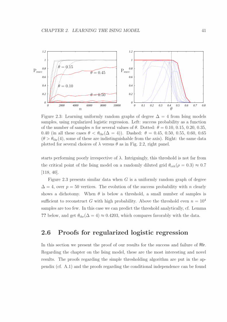
CHAPTER 2. LEARNING THE ISING MODEL 41
0
0.2
0.4
0.6
0.8
1
1.2
0 2000 4000 6000 8000 10000 0
0.2
0.4
0.6
0.8
1
1.2
0 0.1 0.2 0.3 0.4 0.5 0.6 0.7 0.8
Psucc
n
θ = 0.10
θ = 0.15
θ = 0.45
θ = 0.50
θ
Psucc
Figure 2.3: Learning uniformly random graphs of degree ∆ = 4 from Ising modelssamples, using regularized logistic regression. Left: success probability as a functionof the number of samples n for several values of θ. Dotted: θ = 0.10, 0.15, 0.20, 0.35,0.40 (in all these cases θ < θthr(∆ = 4)). Dashed: θ = 0.45, 0.50, 0.55, 0.60, 0.65(θ > θthr(4), some of these are indistinguishable from the axis). Right: the same dataplotted for several choices of λ versus θ as in Fig. 2.2, right panel.
starts performing poorly irrespective of λ. Intriguingly, this threshold is not far from
the critical point of the Ising model on a randomly diluted grid θcrit(ρ = 0.3) ≈ 0.7
[118, 40].
Figure 2.3 presents similar data when G is a uniformly random graph of degree
∆ = 4, over p = 50 vertices. The evolution of the success probability with n clearly
shows a dichotomy. When θ is below a threshold, a small number of samples is
sufficient to reconstruct G with high probability. Above the threshold even n = 104
samples are too few. In this case we can predict the threshold analytically, cf. Lemma
?? below, and get θthr(∆ = 4) ≈ 0.4203, which compares favorably with the data.
2.6 Proofs for regularized logistic regression
In this section we present the proof of our results for the success and failure of Rlr.
Regarding the chapter on the Ising model, these are the most interesting and novel
results. The proofs regarding the simple thresholding algorithm are put in the ap-
pendix (cf. A.1) and the proofs regarding the conditional independence can be found

CHAPTER 2. LEARNING THE ISING MODEL 42
in [21]. The proofs for Rlr were first introduced in [68, 16].
The proof regarding the result on Rlr builds on four lemmas that will be proved in
the appendices. Conceptually, the proof relies on two types of technical results. First,
we estabilish that the incoherence condition introduced in [94] is roughly necessary
for regularized logistic regession to succeed, cf. Lemma 2.6.1. Second, we use this
fact, together with the main result of [94] to characterize the success probability on
three graph families, cf. Lemmas 2.6.2, 2.6.3, 2.6.4. Finally, in order to prove the
negative part in Theorem 2.3.6 we simply construct a graph by taking the disjoint
union of elements from each of these families.
2.6.1 Notation and preliminary remarks
Before proceeding it is convenient to recall some notation and make some preliminary
remarks.
We denote by [m] = 1, 2, . . . , m the set of first m integers. If v ∈ Rm is a vector
and R ⊆ [m] is an index set then vR ≡ (vi)i∈R denotes the vector formed by the
entries with index in R. Similarly, if M ∈ Rm×n is a matrix and R ⊆ [m], P ⊆ [n] are
index sets, then MR,P ≡ (Mij)i∈R,j∈P denotes the submatrix indexed by rows in R
and columns in P . We denote the maximum and minimum eigenvalue of a symmetric
matrixM by σmax(M) and σmin(M) respectively. Recall that ‖M‖∞ = maxi∑
j |Mij |.We denote by 1 the all-ones vector
As before, we let r be the vertex whose neighborhood we are trying to reconstruct
and define S = ∂r and SC = V \(∂r∪r). Since the function Ln(θ; x(ℓ)nℓ=1)+λ‖θ‖1only depends on θ through the components θr,· = θrj : j ∈ V \r (see equation
(2.3.15)), we hereafter neglect all the other parameters and write θ as a shorthand of
θr,·. As mentioned above, whenever necessary to avoid confusion, we will write θ0 or
θ0 (if viewed as a vector) for the true parameters values. Namely θ0 = θrj : θij =
0, ∀j /∈ ∂r, θrj = θ0, ∀j ∈ ∂r.We denote by z0 a sub-gradient of ‖θ‖1 evaluated at the true parameters values
θ0. Note that, since we are working in the ferromagnetic domain, i.e. (θ0S)i > 0
for all i ∈ S, we have z0S = 1. We define W n(θ) to be minus the gradient of Ln,

CHAPTER 2. LEARNING THE ISING MODEL 43
W (θ) to be the minus the gradient of L, Qn(θ) to be the Hessian of Ln(θ) and Q(θ)
to be the Hessian of L(θ). Notice that, by the law of large numbers, for every θ,
limn→∞Ln(θ) = L(θ), limn→∞W n(θ) = W (θ), and limn→∞Qn(θ) = Q(θ).
The gradient and Hessian of L admit indeed fairly explicit expressions. For all
i, j ∈ V \r we have,
Qnij(θ) =
1
n
n∑
ℓ=1
x(ℓ)i x
(ℓ)j
cosh2(∑
t∈V \r θrtx(ℓ)t
) , (2.6.1)
Qij(θ) = EG,θ
(XiXj
cosh2(∑
t∈V \r θrtXt)
), (2.6.2)
−W ni (θ) = [∇Ln(θ)]i =
1
n
n∑
ℓ=1
x(ℓ)i
(tanh
( ∑
t∈V \rθrtx
(ℓ)t
)− x(ℓ)
r
), (2.6.3)
−Wi(θ) = [∇L(θ)]i = EG,θ
Xi tanh
( ∑
t∈V \rθrtXt
)− EG,θXiXr. (2.6.4)
Note that, from the last expression, it follows that ∇L(θ0) = 0. This in turn is related
to asymptotic consistency: if λ → 0 as n → ∞ then θ → θ0.
We let θ denote the parameter estimate computed by Rlr(λ) when applied to
samples x(ℓ)nℓ=1.
We will omit arguments whenever clear from the context. Any quantity evaluated
at the true parameter values will be represented with a 0, e.g. Q0 = Q(θ0). We use
instead a hat (as in θ) to denote estimates based on x(ℓ)nℓ=1. When clear from the
context we might write EG,θ as simply E. Similarly, PG,θ will be sometimes written
as simply P.
Throughout this paper, Psucc will denote the probability of success of Rlr, that is,
the probability that the algorithm is able to recover the underlying G exactly. Also,
G will be a graph of maximum degree ∆.
2.6.2 Necessary conditions for the success of Rlr
Our first technical result establishes that, if λ is small and ‖Q0SCS(Q
0SS)
−1z0S‖∞ > 1,
then Rlr(λ) fails to reconstruct the neighborhood S correctly. (Recall that z0S is the

CHAPTER 2. LEARNING THE ISING MODEL 44
Figure 2.4: Diamond graphs Gdiam(p).
subgradient of ‖θ‖1 evaluated at θ0.) Notice that, under the incoherence condition
‖Q0SCS(Q
0SS)
−1z0S‖∞ ≤ (1 − α)‖z0S‖∞ ≤ (1 − α). Hence this lemma suggests that
incoherence is roughly necessary for regularized logistic regression to succeed. Its
proof can be found in Appendix A.2. (It is not quite necessary because it could in
principle be the case that ‖Q0SCS(Q
0SS)
−1‖∞ > 1 but ‖Q0SCS(Q
0SS)
−1z0S‖∞ < 1.)
Lemma 2.6.1. Assume [Q0SCS(Q
0SS)
−1z0S]i ≥ 1 + ǫ for some ǫ > 0 and some row
i ∈ V , σmin(Q0SS) ≥ Cmin > 0, and λ < C3
minǫ/(27(1 + ǫ2)∆3). Then the success
probability of Rlr(λ) is upper bounded as
PG(λ) = G ≤ 4∆2e−nδ2A + 4∆ e−nλ2δ2B (2.6.5)
where δA = (C2min/32∆)ǫ and δB = (Cmin/64
√∆)ǫ.
2.6.3 Specific graph ensembles
In this section we consider the performances of Rlr(λ) on three graph ensembles.
In the proof of Theorem 2.3.6, we will take the disjoint union of one graph from
each ensemble. This trick allows us to rule out a subset of values of λ for each
graph ensemble. Notice that, in each case, we single out a specific vertex r whose
neighborhood is to be reconstructed. Equivalently, we define here ensembles of rooted
graphs. The three graph ensembles are defined as follows:
One-edge graphs Gone(p). This is the set of graphs with vertex set V = [p] and
only one edge involving the distinguished vertex r, E = (r, i) (e.g. r = 1,
i = 2).
Diamond graph Gdiam(p). This is the set of graphs with p vertices and 2(p − 2)
edges (see Figure 2.4). Two of the vertices to be denoted as vertex 1 and vertex

CHAPTER 2. LEARNING THE ISING MODEL 45
2 have degree (p− 2). They are connected to each of vertices 3, . . . , p which
have in turn degree 2. The maximum degree is ∆ = p− 2. We will identify the
root vertex with r = 1.
These graphs capture a situation in which the two variables interact ‘indirectly’
through numerous weak intermediaries.
Random regular graph Grand(p,∆). Finally we denote by Grand(p,∆) the set of
regular graphs with p nodes and degree ∆. This is naturally endowed with
the uniform probability distribution. With a slight abuse of notation, we shall
use Grand(p,∆) to denote the resulting probability law over graphs, and write
G ∼ Grand(p,∆) for a uniformly random regular graph. The root r is also chosen
uniformly at random in V .
The proof of the first lemma can be found in [16] and the proofs of the two other are
included in Appendices A.4 and A.5.
The first lemma of this section considers one-edge graphs in Gone(p). It implies
that, unless nλ2 is increasing with p, Rlr(λ) fails with significant probability.
Lemma 2.6.2 (One-edge graphs Gone(p)). There exist M = M(K, θ) > 0 decreasing
with K for θ > 0 such that the following is true. If G ∈ Gone(p) and nλ2 ≤ K, then
PG(λ) = G ≤ e−M(K,θ)p + e−n(1−tanh θ)2/32 . (2.6.6)
The same upper bounds holds for the probability of reconstructing the neighborhood of
the root r.
The second lemma deals with diamond graphs Gdiam(p). It shows that Rlr(λ) fails
if λ is bounded away from 0 provided θ∆ ≥ 2.
Lemma 2.6.3 (Diamond graphs Gdiam(p)). There exists ∆0 ≥ 3 (with ∆0 ≤ 50) such
that the following happens for all ∆ ≥ ∆0 and 2 ≤ θ∆ ≤ 3. For any G ∈ Gdiam(p =
∆+ 2) and any fixed λmin > 0,
supλ≥λmin
PG(λ) = G ≤ ǫ for all n > n0(∆, ǫ, λmin) . (2.6.7)
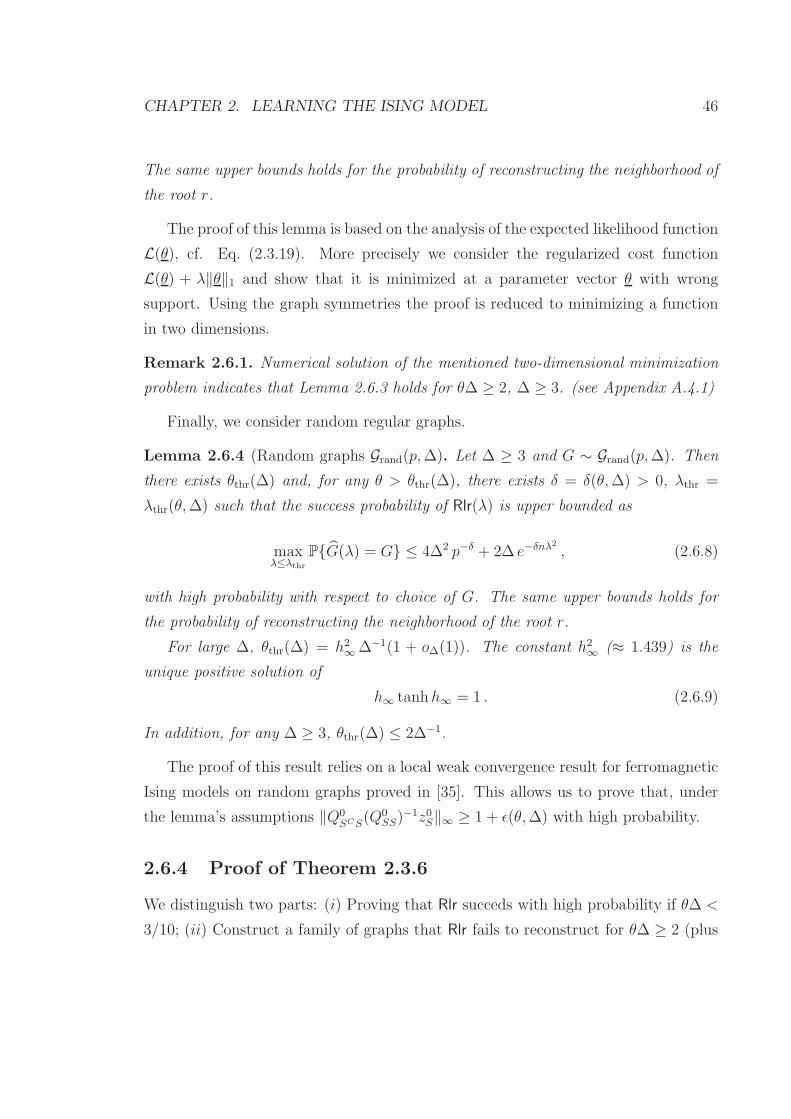
CHAPTER 2. LEARNING THE ISING MODEL 46
The same upper bounds holds for the probability of reconstructing the neighborhood of
the root r.
The proof of this lemma is based on the analysis of the expected likelihood function
L(θ), cf. Eq. (2.3.19). More precisely we consider the regularized cost function
L(θ) + λ‖θ‖1 and show that it is minimized at a parameter vector θ with wrong
support. Using the graph symmetries the proof is reduced to minimizing a function
in two dimensions.
Remark 2.6.1. Numerical solution of the mentioned two-dimensional minimization
problem indicates that Lemma 2.6.3 holds for θ∆ ≥ 2, ∆ ≥ 3. (see Appendix A.4.1)
Finally, we consider random regular graphs.
Lemma 2.6.4 (Random graphs Grand(p,∆). Let ∆ ≥ 3 and G ∼ Grand(p,∆). Then
there exists θthr(∆) and, for any θ > θthr(∆), there exists δ = δ(θ,∆) > 0, λthr =
λthr(θ,∆) such that the success probability of Rlr(λ) is upper bounded as
maxλ≤λthr
PG(λ) = G ≤ 4∆2 p−δ + 2∆ e−δnλ2
, (2.6.8)
with high probability with respect to choice of G. The same upper bounds holds for
the probability of reconstructing the neighborhood of the root r.
For large ∆, θthr(∆) = h2∞∆−1(1 + o∆(1)). The constant h2
∞ (≈ 1.439) is the
unique positive solution of
h∞ tanh h∞ = 1 . (2.6.9)
In addition, for any ∆ ≥ 3, θthr(∆) ≤ 2∆−1.
The proof of this result relies on a local weak convergence result for ferromagnetic
Ising models on random graphs proved in [35]. This allows us to prove that, under
the lemma’s assumptions ‖Q0SCS(Q
0SS)
−1z0S‖∞ ≥ 1 + ǫ(θ,∆) with high probability.
2.6.4 Proof of Theorem 2.3.6
We distinguish two parts: (i) Proving that Rlr succeds with high probability if θ∆ <
3/10; (ii) Construct a family of graphs that Rlr fails to reconstruct for θ∆ ≥ 2 (plus

CHAPTER 2. LEARNING THE ISING MODEL 47
the mentioned conditions).
The second part is the most challenging technically, and builds on Lemmas 2.6.2,
2.6.3, 2.6.4.
2.6.5 Proof of Theorem 2.3.6: θ∆ ≤ 3/10
The proof consists in checking the sufficient conditions for the success of Rlr described
in [94, Theorem 1] hold true. Namely we prove the following Lemma.
Lemma 2.6.5. For θ∆ ≤ 3/10, there exists constants Cmin > 0, Dmax < ∞ and
α < 1 such that
σmin(Q0SS) > Cmin, (2.6.10)
σmax(EG,θ(XSX∗S)) < Dmax, (2.6.11)
‖Q0SCS(Q
0SS)
−1‖∞ ≤ 1− α. (2.6.12)
This is proved in Appendix A.3 by estabilishing estimates on the entries Q0 using
a technique of Fisher [40]. Once this lemma is established, the upper-bound on the
sample-complexity follows by carefully carrying all the proofs in [94, Theorem 1]
without dropping any constants.
2.6.6 Proof of Theorem 2.3.6: θ∆ ≥ 2
First consider the last part of the Theorem, cf. Eq. (2.3.18). By Lemma 2.6.4, we
have
maxλ∈[λ1(p)/
√n,λ2(n)]
PG(λ) = G ≤ 4∆2 p−δ + 2∆ e−δλ1(p)2) ,
for all but a vanishing fraction of graphs G ∈ Grand(p,∆). Since δ > 0 and λ1(p) → ∞as p → ∞, the right hand side will be smaller than ǫ for all p large enough. Therefore,
maxλ∈[λ1(p)/
√n,λ2(n)]
PG(λ) = G ≤ ǫ , for all n ∈ N,
for all but a vanishing fraction of graphs G ∈ Grand(p,∆).
CHAPTER 2. LEARNING THE ISING MODEL 48
Next consider the claim (2.3.17). Fix ∆ ≥ ∆0, whereby ∆0 is defined in such a
way that Lemma 2.6.3 holds, and θ so that 2 ≤ θ∆ ≤ 3. We construct a graph G
with ptot = 2p + (∆ + 2) vertices as a disjoint union of G = G1 ∪ G2 ∪ G3. Here
G1 = (V1, E1) ∈ Gone(p) is a one-edge graph with p vertices and root r1; G2 =
(V2, E2) ∈ Gdiam(∆ + 2) is a diamond graph with ∆ + 2 vertices and root r2; G3 =
(V3, E3) ∼ Grand(p,∆) is a uniformly random regular graph with degree ∆, rooted at
r3. It is sufficient to prove that, for all n large enough
supλ∈R+
PG,θ,n(G(λ) = G) ≤ 1
2.
For ℓ ∈ 1, 2, 3, let Eℓ(λ) be the event that Rlr(λ) reconstructs the neighborhood
of rℓ correctly. Further let E0(λ) be the event that Rlr(λ) does not return any edge
across vertex sets V1, V2, V3 (such edges are absent from the ground truth). We then
have
supλ∈R+
P(G(λ) = G) ≤ supλ∈R+
minP(E1(λ) ∩ E0(λ)); P(E2(λ) ∩ E0(λ)); P(E3(λ) ∩ E0(λ))
It is therefore sufficient to show that there exists a function p 7→ λ1(p) and a constant
λ2 > 0 such that, with positive probability with respect to the choice of the random
graph G, we have
supλ∈[0,λ1(p)/
√n]
P(E1(λ) ∩ E0(λ)) ≤ 1
2,
supλ∈[λ1(p)/
√n,λ2]
P(E3(λ) ∩ E0(λ)) ≤ 1
2,
supλ∈[λ2,∞)
P(E2(λ) ∩ E0(λ)) ≤ 1
2.
We fix the function p 7→ λ1(p) such that λ1(p) → ∞ as p → ∞ and M(λ1(p)2, θ)p ≥
log p, where M(· · · ) is defined as per Lemma 2.6.2. This is possible since M(K, θ) is
decreasing and strictly positive at any K < ∞.
Notice that, under E0(λ), Rlr(λ) outputs θr1,j = 0 for any j ∈ V2 ∪ V3. We can
therefore bound P(E1(λ) ∩ E0(λ)) as if G2 and G3 were absent. Using Lemma 2.6.2

CHAPTER 2. LEARNING THE ISING MODEL 49
we get
supλ∈[0,λ1(p)/
√n]
P(E1(λ) ∩ E0(λ)) ≤ e−M(λ1(p)2,θ)p + e−n(1−tanh θ)2/32
≤ 1
p+ e−n(1−tanh θ)2/32 ≤ 1
2,
where the last inequality follows for p ≥ 4 and n ≥ 64/(1− tanh θ)2.
Analogously, we can use Lemma 2.6.4 to upper bound the probability of E3(λ).We get, for δ = δ(θ,∆) > 0,
supλ∈[λ1(p)/
√n,λ2]
P(E3(λ) ∩ E0(λ)) ≤ 4∆2 p−δ + 2∆ e−δnλ2
≤ 4∆2 p−δ + 2∆ e−δλ1(p)2 ≤ 1
2,
where the last inequality follows for p ≥ p0(∆, θ).
Finally, using Lemma 2.6.3 we obtain the desired bound on P(E2(λ) ∩ E0(λ)), forn > n0(∆, 1/2, λ2).
2.6.7 Discussion
The construction used in the proof of Theorem 2.3.6 for θ∆ > 2 might appear some-
what contrived. In reality it exposes quite clearly the basic mechanisms at work.
First of all, it is necessary to scale λ ≥√λ1(p)/n, with λ1(p) → ∞. Indeed, if
this is not the case, Rlr(λ) will fail reconstructing the neighborhood of any vertex that
is connected only to a few neighbors, and essentially independent from most other
vertices. This phenomenon is independent of the tradeoff between ∆ and θ, and of
the correlation decay properties. The graph G1 ∈ Gone(p) is only a particularly simple
example that demonstrates it.
On the other hand we expect that, to demonstrat failure of Rlr(λ) for λ ≥√λ1(p)/n, either of the two graphs G2 ∈ Gdiam(∆ + 2) or G3 ∼ Grand(p,∆) should
be sufficient. The main reason to use the disjoint union of G2 and G3 is that each
of the two cases is easier to treat in a distinct regime. Further, each of the two

CHAPTER 2. LEARNING THE ISING MODEL 50
types of graphs is interesting in its own. While G2 ∈ Gdiam(∆ + 2) is extremely sim-
ple, G3 ∼ Grand(p,∆) is ‘typical’ (as it reproduces the behavior of most graphs with
degree ∆).
The insight associated to failure on Gdiam(∆ + 2) or Grand(p,∆) is similar. Strong
correlations between vertices that are not directly connected fool the algorithm.
2.7 Regularized logistic regression and graph fam-
ilies with additional structure
Our main result concerning Rlr, Theorem 2.3.6, implies that regularized logistic re-
gression generally fails when ∆max(ij)∈E |θij| ≥ 2. It is natural to wonder whether
this conclusion changes under additional assumptions on the graph G.
The next result is a striking example of this type.
Proposition 2.7.1. If G is a tree with maximum degree ∆ then, for any θ > 0,
NRlr(G, θ) ≤ C∆
θ2log(pδ
). (2.7.1)
The proof of this proposition is obtained by showing that, for any θ,∆, the Ising
measure on a tree G with maximum degree ∆ satisfies the incoherence condition. The
proof of this proposition can be found in the appendix of [67].
The last statement might appear to contradict Lemma 2.6.4. The proof of the
latter is based on the local weak convergence of the distribution (2.1.1) for random
regular graph to an Ising measure on a regular tree. For the latter measure, we prove
that the incoherence condition is violated for ∆θ large enough.
Remark 2.7.1. There is no contradiction between Proposition 2.7.1 and Lemma
2.6.4. The Ising measure on a random regular graph converges to the measure on a
tree with plus boundary conditions. The relevant measure for a finite tree, used in
Proposition 2.7.1 has free boundary conditions.
Our last example concerns loopy graphs, namely two dimensional grids. It implies

CHAPTER 2. LEARNING THE ISING MODEL 51
that Rlr(λ) fails above a certain threshold in θ: in this case, additional structure does
not change the qualitative conclusion of Theorem 2.3.6.
Proposition 2.7.2. There exists θ2d such that the following happens for all θ > θ2d.
Let G be a two-dimensional grid of size√p × √
p with periodic boudary condition,
and, p 7→ λ1(p) and n 7→ λ2(n) be such that λ1(p) → ∞ as p → ∞ and λ2(n) → 0 as
n → ∞. Then for any ǫ > 0 there esist p0, n0 such that, if p ≥ p0, n ≥ n0, then
supλ∈[λ1(p)/
√n,λ2(d)]
PG,θ,n(G(λ) = G) ≤ ǫ .
The proof uses once more Lemma 2.6.1 and shows that the incoherence condition
is violated at large enough θ. The proof of this fact is very technical and can be found
in the appendix of [67].
Assuming λ ∈ [λ1(p)/√n, λ2(d)] is natural for the same reasons as explained after
the statement of Theorem 2.3.6.

Chapter 3
Learning stochastic differential
equations
In this chapter we study the sample-complexity and computational-complexity in
learning graphical models from data with correlations. The focus is on stochastic
differential equations (SDEs) and learning from continuous trajectories. A specific
type of SDE already appeared in the Introduction (Chapter 1 equation (1.2.5)): in
linear SDEs the rate of change of each variable is a linear combination of neighboring
variables in a graph G. However, our interest is broader, and in Section 3.1, a very
general family of non-linear SDEs parametrized by graphs is introduced and is then
analyzed throughout the chapter.
An ℓ1-regularized least-squares algorithm to learn these non-linear SDEs is dis-
cussed in Section 3.3.2. We denote it by Rls. Our main results (Section 3.3) charac-
terize the sample-complexity of Rls in learning linear SDEs with sparse representation
from continuous trajectories. A general result is presented in Section 3.3.3, and, to
facilitate its interpretation, in Section 3.3.4 we look at the simpler case of linear SDEs
parametrized by the Laplacian of a graph. In Section 3.5, we study two essential re-
sults that are the basis of our main results. Namely, in Section 3.5.1, we focus on
52

CHAPTER 3. LEARNING STOCHASTIC DIFFERENTIAL EQUATIONS 53
learning stochastic linear difference equations 1 – of which learning SDEs from con-
tinuous trajectories is a limiting case – and in Section 3.5.2, we describe a general
lower bound on the sample-complexity of learning SDEs – from which we derive a
lower bound matching the upper bound on the sample-complexity of Rls. In Section
3.7.1, we look at a lower bound on the sample-complexity of learning dense linear
SDEs and in Section 3.7.2 at a lower bound when learning non-linear SDEs.
Our results show that the presence of correlations in the samples is balanced by the
infinite number of data points from the continuous trajectories and results in a change
of the sample-complexity (regarding the dependency in p) only by a multiplicative
factor in comparison with when samples are independent. Why is this so and what
is this multiplicative factor?
Let us look at the autocorrelation function of the sampled stationary trajectory
of the following 1-D linear SDE
dx(t) = −ρx(t)dt + db(t). (3.0.1)
For ρ > 0 the SDE admits a unique stationary solution [88] and we obtain
Ex(0)x(ℓη) =1
2ρe−ρℓη. (3.0.2)
If η ≫ 1/ρ, consecutive samples are approximately independent. From a different
perspective, in n samples spaced in time by η, the number of approximately inde-
pendent samples is O(nmin1, ηρ). Hence, for example, if learning sparse graphs
of bounded degree ∆ from n independent samples can be, in principle, done for
n < O(∆ log p) [21], then learning sparse graphs for SDEs should be possible for
n < O(∆max1, (ηρ)−1 log p). Since nη is the length T of the observation window
of the trajectory, we can write T < O(∆maxη, ρ−1 log p). As η → 0, the bound
converges to T < O(∆ρ−1 log p) and it is tempting to regard this metric as a bound
on the sample complexity when learning from continuous time data. In particular,
1Throughout this thesis we often refer to stochastic difference equations as linear SDEs in discretetime. A simple example of a linear SDE in discrete time is x(n + 1) = 0.5x(n) + w(n), n = 0, 1, ...where x(0) = 0 and w(n)∞n=0 are i.i.d. N(0,1) random variables.

CHAPTER 3. LEARNING STOCHASTIC DIFFERENTIAL EQUATIONS 54
this bound predicts that the smaller ρ is, the more information we need to learn G.
In this section we show the above relation between η, n and ρ is partially correct.
More precisely, we prove an upper bound that is similar to the bounds for independent
samples and behaves like ρ−1 for ρ small. In our result, ρ is the decay rate of the
slowest mode of the SDE. In other words, Rls performs worse as the SDE approaches
instability. However, the same upper-bound also predicts that, as ρ increases, the
sample-complexity degrades. This is at odds with the bound we obtained here but
is the correct behavior. In fact, this is the best possible behavior for ρ large since,
for this regime, we can prove a matching lower bound for any algorithm with success
probability greater than 1/2. To understand this, look at the SDE as a dynamical
system driven by white-noise. For ρ large, the system quickly filters any inputs and
the driving white-noise cannot excite the system enough for us to learn it from data.
The question of characterizing the sample-complexity of learning from a sampled
continuous trajectory remains open (but see Section 3.2 for an overview on related
work).
The work in this chapter is based on joint work with Ibrahimi and Montanari
[14, 15, 13].
3.1 Introduction
Consider a continuous-time stochastic process x(t)t≥0, x(t) = [x1(t), . . . , xp(t)] ∈R
p, which is defined by a stochastic differential equation (SDE) of diffusion type
dx(t) = F (x(t); θ0) dt+ db(t) , (3.1.1)
where b(t) is a p-dimensional standard Brownian motion and the drift coefficient 2,
F (x(t); θ0) = [F1(x(t); θ0), . . . , Fp(x(t); θ
0)] ∈ Rp, is a function of x(t) parametrized
by θ0. This is an unknown vector, with dimensions scaling polynomially with p.
In this chapter we consider the problem of learning the support of the vector θ0
2Throughout this chapter, vectors are ‘column vector’ even if they are represented in row formfor typographical reasons.

CHAPTER 3. LEARNING STOCHASTIC DIFFERENTIAL EQUATIONS 55
from a sample trajectory XT0 ≡ x(t) : t ∈ [0, T ]. More precisely, we focus on
the high-dimensional limit, where p can grow with T , and determine necessary and
sufficient conditions for recovering the signed support of θ0 with high probability 3.
As stated in the introductory Chapter 1, we refer to the smallest T that allows us
to achieve a prescribed success probability as the ‘sample-complexity’ of the problem
(although the number of samples is, strictly speaking, infinite). We are particularly
interested in achieving the optimal scaling of sample-complexity with the problem
dimensions through computationally efficient procedures.
Concretely, given a SDE parametrized by θ0 and an algorithm Alg = Alg(XT0 ) that
outputs an estimate θ, we define the sample-complexity TAlg(θ0) as
TAlg(θ0) = infT0 ∈ R
+ : Pθ0,Tsign(θ) = sign(θ0) ≥ 1− δ for all T ≥ T0. (3.1.2)
In the expression above, Pθ0,T denotes probability with respect to the trajectory XT0 .
Obviously, TAlg(θ0) defined above is an upper bound for sample-complexity of learning
the support alone.
In addition to this definition, given a class of A of parameters we define,
TAlg(A) = maxΘ0∈A
TAlg(θ0). (3.1.3)
Models based on SDEs play a crucial role in several domains of science and technol-
ogy, ranging from chemistry to finance. Correspondingly, parameter estimation has
been intensely studied in this context. We refer to Section 3.2 for a brief overview.
A complete understanding of parameter estimation in a high-dimensional setting is
nevertheless missing.
Our results address these challenges for special classes of SDEs of immediate rele-
vance. A first class is constituted by drift coefficients that are parametrized linearly.
3Recall that the signed support of θ0 is represented by sign(θ0) and corresponds to the partitionof the set of indices of θ0 into three sets: indices with positive value, indices with negative value andindices with zero value.

CHAPTER 3. LEARNING STOCHASTIC DIFFERENTIAL EQUATIONS 56
Explicitly, we are given a set of basis functions
F (x) = [f1(x), f2(x), . . . , fm(x)], (3.1.4)
with fi : Rp → R. The drift is then given as F (x; Θ0) = Θ0F (x), with Θ0 ≡
(θ0ij)i∈[p],j∈[m] ∈ Rp×m. In this chapter we often use the notation Θ0 instead of θ0 to
stress that the unknown parameter has a natural matrix presentation. We then have,
for each i ∈ Rp,
dxi(t) =m∑
j=1
θ0ijfj(x(t)) dt+ dbi(t) . (3.1.5)
Suitable sets of basis functions can be provided by domain-specific knowledge. As
an example, within stochastic models of chemical reactions, the drift coefficient is
a low-degree polynomial. For instance, the reaction A + 2B → C is modeled as
dxC = kC,ABxAx2Bdt + dbC, where xA, xB and xC denote the concentration of the
species A, B and C respectively, and dbC is a chemical noise term. In order to learn
a model of this type, one can consider a basis of functions F (x) that comprises all
monomials up to a maximum degree.
An important subclass of models of the last type is provided by linear SDEs.
In this case, the drift is a linear function of x(t), namely F (x; Θ0) = Θ0x(t) with
Θ0 ≡ (θ0ij)i,j∈[p] ∈ Rp×p. Explicitly, for each i ∈ R
p,
dxi(t) =
p∑
j=1
θ0ijxj(t) dt+ dbi(t) . (3.1.6)
A model of this type is a good approximation for many systems near a stable equi-
librium. The model (3.1.6) can be used to trace fluctuations of the species’ concen-
trations in proximity to an equilibrium point. The matrix Θ0 would represent in this
case the linearized interactions between different chemical factors.
More generally, we can associate to the model (3.1.6) a directed graph G = (V,E)
with edge weight θ0ij ∈ R associated with the directed edge (j, i) from j ∈ V to i ∈ V .
Each component xi(t) of the vector x(t) describes the state of a node i ∈ V . The
graph G describes which nodes interact: the rate of change of xi(t) is given by a

CHAPTER 3. LEARNING STOCHASTIC DIFFERENTIAL EQUATIONS 57
weighted sum of the current values of its neighbors, corrupted by white noise. In
other words linear SDE’s can be seen as graphical models – a probabilistic model
parametrized by a graph.
This thesis establishes lower bounds on the sample-complexity for estimating the
general model (3.1.1). These bounds are based on information theoretic techniques
and apply irrespective of computational considerations. For linear models of the form
(3.1.6), we put forward a low-complexity estimator and derive upper bounds on its
sample-complexity. Upper and lower bounds are shown to be within a constant factor
for special classes of sparse networks Θ0.
3.2 Related work
The problem of estimating the parameters of a diffusion plays a central role in several
applied domains, the most notable being econometrics, chemistry and system biology.
In the first context, diffusions are used to model the evolution of price indices
[92]. While the most elementary process is the (geometric) Brownian motion [10, 19],
a number of parametric families have been introduced to account for nonlinearities.
The number of parameters is usually small and parameter estimation is addressed via
maximum likelihood (ML). We refer to [12, 76] for proofs of consistency and asymp-
totic normality of the ML estimator. Much of the recent research has focused on
dealing with the challenges posed by the fact that the diffusion is sampled at discrete
intervals, and the transition probabilities cannot be computed in closed form. A short
list of contributions on this problem includes [31, 91, 5]. In particular, asymptoti-
cally consistent methods based on approximate transition probabilities exist, see for
instance [90, 26]. Nonparametric estimation of the drift coefficient has been studied
as well [39, 104, 32].
Let us emphasize that all of these works focus on the low-dimensional setting: the
vector of parameters to be estimated is p-dimensional, and the diffusion is observed
for a time T → ∞. Hence there is little overlap with the present work. In particular,
simple ML estimators are not viable in the high-dimensional setting. At the same
time, it would be interesting to address the problems posed by discrete sampling and

CHAPTER 3. LEARNING STOCHASTIC DIFFERENTIAL EQUATIONS 58
non-parametric estimation in the high-dimensional setting as well.
Applications to chemistry and system biology have been mentioned in Section
3.1. A large variety of chemical reaction is modeled by diffusions with suitably
parametrized drift terms [54, 60]. Of particular interest here are special classes of
drift coefficients, for instance those exhibiting time-scale separation [89] or gradients
of a potential [93]. As for econometrics applications, these works have focused on
low-dimensional diffusions.
Technically, our work fits on recent developments in learning high-dimensional
graphical models. The typical setting assumes that the data are i.i.d. samples from a
high-dimensional Gaussian distribution with sparse inverse covariance. The underly-
ing graph structure (the support of the inverse covariance) is estimated using convex
regularizations that promote sparsity. Well known examples include the graphical
LASSO [44] and the pseudo-likelihood method of [81]. In the context of binary pair-
wise graphical models, similar methods were developed in Ref. [110]. To the best of
our knowledge the work described by this thesis is the first one moving beyond the
assumption of i.i.d. samples. While we extend ideas and methods from this literature,
dealing with dependent samples raises new mathematical challenges.
Our methods build on the work on ℓ1-regularized least squares, and its variants
[107, 36, 37, 115, 109]. The most closely related results are the one concerning high-
dimensional consistency for support recovery [81, 110, 116]. Our proof for our upper
bound follows indeed the approach developed in these papers, with two important
challenges. First, the design matrix is in our case produced by a stochastic diffu-
sion, and it does not necessarily satisfies the irrepresentability conditions used by
these works. Second, the observations are not independent and therefore elementary
concentration inequalities are not sufficient.
Most of these proofs build on the technique of [116]. A naive adaptation to the
present case allows to prove some performance guarantee for the discrete-time setting.
However the resulting bounds are not uniform as the sampling interval η tends to
0 for nη = T fixed. In particular, they do not allow to prove an analogous of our
continuous time result, Theorem 3.3.1. A large part of our effort is devoted to proving
more accurate probability estimates that capture the correct scaling for small η.

CHAPTER 3. LEARNING STOCHASTIC DIFFERENTIAL EQUATIONS 59
Finally, the related topic of learning graphical models for autoregressive processes
was studied recently in [102, 103]. These papers propose a convex relaxation that
is different from the one studied in this paper, without however estabilishing high-
dimensional consistency for model selection.
Preliminary report of our work were presented at NIPS 2010 [14] and ISIT 2011
[15]. Subsequent work by Bolstad, Van Veen and Nowak [20] establishes high-dimensional
consistency for estimating autoregressive models through a related approach. These
guarantees are non-uniform in the sampling rate η.
3.3 Main results
Our main contributions are the following:
Information-theoretic lower bound. We establish a general lower bound on the
sample complexity for estimating the signed support of the drift coefficient of a
diffusion of the form (3.1.1). By specializing this result, we obtain bounds for
the linearly parametrized model (3.1.5), and the linear model (3.1.6).
Upper bound via penalized least squares. For the linear model (3.1.6), and suit-
able classes of sparse matrices Θ0, we prove high-dimensional consistency of the
penalized least-squares method introduced in Section 3.3.2. The resulting upper
bound on sample complexity matches the information theoretic lower bound up
to constant factors.
In this section we focus on the case of sparse linear SDE’s, stating upper and lower
bounds in this case, cf. Section 3.3.3. We then illustrate the general theory by
analyzing a specific but rich problem: learning the Laplacian of a sparse graph, cf.
Section 3.3.4.
Related results extending the ones presented here (in particular, general lower
bounds on the sample complexity) are discussed in Section 3.5 and in Section 3.7.

CHAPTER 3. LEARNING STOCHASTIC DIFFERENTIAL EQUATIONS 60
3.3.1 Notation
Let us recall some important notation is used in this chapter.
For N ∈ N, we let [N ] = 1, 2, . . . , q. Given a matrix Q, its transpose is denoted
by Q∗ and its support supp(Q) is the 0 − 1 matrix such that supp(Q)ij = 1 if and
only if Qij 6= 0. The support supp(v) is defined analogously for a vector v ∈ RN .
With a slight abuse of notation, we occasionally write supp(v) for the subset of indices
i ∈ [N ] such that vi 6= 0. The signed support of a matrix (or vector) Q, denoted by
sign(Q), is the matrix defined by sign(Q)ij = sign(Qij) if Qij 6= 0 and sign(Q)ij = 0
otherwise. The r-th row of a matrix Q is denoted by Qr.
Given a matrix Q ∈ RM×N , and sets L ⊆ [M ], R ⊆ [N ], we denote by QL,R the
sub-matrix QL,R ≡ (Qij)i∈L,j∈R.
For q ≥ 1, the ℓq norm of a vector v ∈ RN is given by ‖v‖q ≡ (
∑i∈[N ] |vi|q)1/q.
This is extended in the usual way to q = ∞. As usual, the misnomer ‘0-norm’ is used
for the size of the support ov v, namely ‖v‖0 is the number of non-zero entries of v.
The ℓq operator norm of a matrix Q ∈ RM×N is denoted by |||Q|||q. In fact, we only
use the ℓ∞ operator norm, which is given by |||Q|||∞ ≡ maxr∈[M ] ‖Qr‖1.If Q ∈ R
N×N is symmetric, then its eigenvalues are denoted by λ1(Q) ≤ λ2(Q) ≤· · · ≤ λN(Q). The minimum and maximum eigenvalues are also denoted as λmin(Q) ≡λ1(Q) and λmax(Q) ≡ λN(Q). For a general (non-symmetric) matrix Q ∈ R
M×N we
let 0 ≤ σ1(Q) ≤ · · · ≤ σM∧N (Q) denote its singular values. Further σmin(Q) = σ1(Q)
and σmax(Q) = σM∧N (Q) are the minimum and maximum singular values.
Throughout this chapter, we denote by C, C1, C2, etc, constants that can be
adjusted from point to point.
3.3.2 Regularized least squares
Before introducing the upper bounds for the sample-complexity of learning SDEs we
must introduce the algorithm with which we achieve them.
Regularized least squares is an efficient and well-studied method for support recov-
ery. In order to describe its application to estimating the signed support of the drift co-
efficient of a high-dimensional diffusion, we consider the general linearly parametrized

CHAPTER 3. LEARNING STOCHASTIC DIFFERENTIAL EQUATIONS 61
model (3.1.5).
We estimate independently each row of the matrix Θ0 ∈ Rp×m. The rth row,
denoted by Θ0r, is estimated by solving the following convex optimization problem
minΘr∈Rp
L(Θr; x(t)t∈[0,T ]) + λ‖Θr‖1 , (3.3.1)
where the log-likelihood function L is defined by
L(Θr; x(t)t∈[0,T ]) =1
2T
∫ T
0
〈Θr, F (x(t))〉2 dt− 1
T
∫ T
0
〈Θr, F (x(t))〉 dxr(t) . (3.3.2)
(Here and below 〈u, v〉 denotes the standard scalar product of vectors u, v ∈ RN .).
We denote this algorithm by Rls(λ).
Notice that in Chapter 2 we used two different notations (Ln and L) to distinguish
the likelihood function when n < ∞ from when n = ∞. In this chapter, L always
represents the case T < ∞.
The ℓ1 regularization term in Eq. (3.3.1) has the role of shrinking to 0 all the
entries θrj , except the most significant ones, thus effectively selecting the support of
Θ.
The normalized log-likelihood function (3.3.2) is the appropriate generalization of
the sum of square residuals for a continuous-time process. To see this heuristically,
one can formally write xr(t) = dxr(t)/dt. A naive sum of square residuals would take
the form∫(〈Θr, F (x(t))〉 − xr(t))
2dt. Unfortunately, this expression is not defined
because xr(t) is not differentiable. On the other hand, expanding the square, we get
2TL(Θr; x(t)[0,T ]) +∫(xr(t))
2dt. The first term is well defined, as is clear from
Eq. (3.3.2), and the second is independent of Θ and hence can be dropped.
Notice that constructing a well-defined cost function as in Eq. (3.3.2) is not a
purely academic problem. Indeed, a cost function that included the time derivative
x(t) would in practice require to estimate x(t) itself. This is all but hopeless because
x(t) does not exist in the model.

CHAPTER 3. LEARNING STOCHASTIC DIFFERENTIAL EQUATIONS 62
3.3.3 Sample complexity for sparse linear SDE’s
In order to state our results, it is convenient to define the class of sparse matrices
A(S), depending on parameters ∆, p ∈ N, ∆ ≥ 3, θmin, ρmin > 0
A(S) = A(S)(∆, p, θmin, ρmin) ⊆ Rp×p (3.3.3)
by letting Θ ∈ A(S) if and only if
(i) ‖Θr‖0 ≤ ∆ for all r ∈ [p].
(ii) |θij| ≥ θmin for all i, j ∈ [p] such that θij 6= 0.
(iii) λmin(−(Θ + Θ∗)/2) ≥ ρmin > 0.
Notice in particular that condition (iii) implies that the system of linear ordinary
differential equations x(t) = Θx(t) is stable. Equivalently, the spectrum of Θ is
contained in the half plane z ∈ C : Re(z) < 0. As a consequence, if Θ0 ∈ A(S),
then the diffusion process (3.1.6) has a unique stationary measure which is Gaussian
with covariance Q0 ∈ Rp×p and is given by the unique solution of Lyapunov’s equation
[117]
Θ0Q0 +Q0(Θ0)∗ + I = 0. (3.3.4)
Hence XT0 = x(t) : t ∈ [0, T ] is stationary trajectory distributed according to the
linear model (3.1.6) if x(t = 0) ∼ N(0, Q0) is a Gaussian random variable independent
of b(t).
We consider the linear model (3.1.6) with Θ0 ∈ A(S). Considering a row index
r ∈ [p], let S0 = S0(r) be the support of Θ0r.
Assumption 1 (Restricted convexity). For Cmin > 0, we have
λmin(Q0S0,S0) ≥ Cmin . (3.3.5)
Assumption 2 (Irrepresentability). For some α > 0, we have
|||Q0(S0)C ,S0
(Q0
S0,S0
)−1 |||∞ ≤ 1− α . (3.3.6)
CHAPTER 3. LEARNING STOCHASTIC DIFFERENTIAL EQUATIONS 63
We refer to [116, 81] for the original development of these conditions in the context
of sparse regression.
Our first theorem establishes high-dimensional consistency of ℓ1-penalized least
squares for estimating sign(Θ0) from a stationary trajectory XT0 according to the
linear model (3.1.6) when Θ0 ∈ A(S). The details of its proof can be found in Section
3.5 and Appendix B.5. In particular in Appendix B.5.
Theorem 3.3.1. If Θ0 ∈ A(S)(∆, p, θmin, ρmin) satisfies assumptions 1 and 2 above
for all r ∈ [p] and some Cmin, α > 0, then there exists λ = λ(T ) such that
TRls(λ)(Θ0) ≤ 2 · 104∆2(∆ ρ−2
min + θ−2min)
α2ρminC2min
log(4p∆
δ
). (3.3.7)
In particular, one can choose
λ =
√36
Tα2ρminlog(4pδ
). (3.3.8)
Remark 3.3.1. Note that our notion of sample-complexity is well-defined for re-
construction algorithms that depend on T , the length of the stationary trajectory XT0 .
This is the case with the regularized least squares algorithm Rlr(λ), since λ can depend
on T .
Corollary 3.3.2. If there exists Cmin, α > 0 such that assumptions 1 and 2 hold for
all r ∈ [p] and for all Θ0 ∈ A(S)(∆, p, θmin, ρmin), then we can replace TRls(λ)(Θ0) by
TRls(λ)(A(S)) in (3.3.7).
The next theorem establishes a lower bound on the sample complexity of learning
the signed support of Θ0 ∈ A(S) from a stationary trajectory, XT0 , distributed accord-
ing to the linear model (3.1.6). The details of the proof of this theorem can be found
in appendix B.6. In particular, in appendix B.6.2.
Theorem 3.3.3. Let Alg = Alg(XT0 ) be an estimator of sign(Θ0). There is a constant
C(∆, δ), such that, for all p large enough,
TAlg(A(S)) ≥ C(∆, δ) maxρmin
θ2min
,1
θmin
log p . (3.3.9)

CHAPTER 3. LEARNING STOCHASTIC DIFFERENTIAL EQUATIONS 64
The last two theorems establish that, under assumptions 1 and 2 above, the time
complexity of learning the support of the diffusion coefficient for sparse linear SDEs
in the class A(S) is of order log p.
Notice that both upper and lower bounds depend in a non-trivial way on the
parameter ρmin. In order to gain intuition on this quantity, consider Eq. (3.1.6) in
absence of the driving term dbi(t). By using the Lyapunov function ‖x(t)‖22, it is easyto verify that ‖x(t)‖2 ≤ ‖x(0)‖2 e−ρmint/2. Hence ρ−1
min provides a general upper bound
on the mixing time of the diffusion (3.1.6). The upper bound is essentially tight if
the matrix Θ0 is symmetric.
Theorems 3.3.1 and 3.3.3 can therefore be used to characterize the dependence
of the sample complexity on the mixing time. One subtle aspect is that Cmin and
ρmin cannot be varied independently because of the Lyapunov equation, Eq. (3.3.4).
In order to clarify this dependency, we apply our general results to the problem of
learning the Laplacian of an undirected graph.
3.3.4 Learning the laplacian of graphs with bounded degree
Given a simple graph G = (V,E) on vertex set V = [p], its Laplacian ∆G is the
symmetric p × p matrix which is equal to the adjacency matrix of G outside the
diagonal, and with entries ∆Gii = −deg(i) on the diagonal [27]. (Here deg(i) denotes
the degree of vertex i.)
It is well known that ∆G is negative semidefinite, with one eigenvalue equal to 0,
whose multiplicity is equal to the number of connected components of G. The matrix
Θ0 = −mI +∆G fits into the setting of Theorem 3.3.1 for m > 0. The corresponding
model (3.1.6) describes the over-damped dynamics of a network of masses connected
by springs of unit strength, and connected by a spring of strength m to the origin.
Let Gbounded = Gbounded(∆, p) be the class of graphs on p nodes with maximum
vertex degree bounded by ∆. Define,
A(L)(m, p,∆) = Θ0 : Θ0 = −mI +∆G, st. m > 0, G ∈ Gbounded (3.3.10)
The following result holds. Its proof can be found in the appendix of [14, 13].
CHAPTER 3. LEARNING STOCHASTIC DIFFERENTIAL EQUATIONS 65
Theorem 3.3.4. Consider the model (3.1.6) with Θ0 ∈ A(L)(m, p,∆). Then there
exists λ such that
TRls(λ)(A(L)) ≤ 4 · 105∆2(∆+m
m
)5(∆ +m2) log
(4p∆δ
), (3.3.11)
In particular one can take, λ =√
36(∆ +m)2 log(4p/δ)/(Tm3).
In other words, for m bounded away from 0 and ∞, regularized least squares
regression correctly reconstructs the graph G from a trajectory of time length which
is polynomial in the degree and logarithmic in the graph size.
Using this theorem we can write the following corollary that helps compare the
bounds obtained in Theorems 3.3.1 and 3.3.3 above.
Corollary 3.3.5. Assume the same setting as in Theorem 3.3.4. There exist con-
stants λ = λ(T ), C1 = C1(∆, δ) and C2 = C2(∆, δ) such that, for all p large enough,
m < ∆ ⇒ C1 log p ≤ TRls(λ)(A(L)) ≤ C2m−5 log p, (3.3.12)
m ≥ ∆ ⇒ C1m log p ≤ TRls(λ)(A(L)) ≤ C2m2 log p . (3.3.13)
In addition, the lower-bounds hold regardless of the choice of λ.
Proof. The proof of this corollary follows immediately from Theorem 3.3.4 and The-
orem 3.3.3.
Notice that the upper bound on TRlr presents a non-trivial behavior in m. It
diverges both at largem, and at small m. The reasons of these behaviors are different.
For smallm, the mixing time of the diffusion (which is proportional to 1/m) gets large,
and hence a large time is necessary to accumulate information about Θ0. Vice-versa
for largem, Θ0 gets close to −mI and hence it depends weakly on the graph structure.
Notice that the lower bound also diverges as m → ∞, hence confirming the above
picture. On the other hand, the behavior of TRls as m → 0 remains an open question
since our lower bound stays bounded in that limit.

CHAPTER 3. LEARNING STOCHASTIC DIFFERENTIAL EQUATIONS 66
3.4 Important remark
Given that Rls(λ) can be tuned using λ, it is natural to asks whether we can write
the above results in a from resembling Theorem 2.3.6 of Chapter 2 for Rlr(λ). In
particular, if we define
TRls(Θ0) = infT0 ∈ R
+ : supλ>0
PΘ0,TRls(λ) = sign(Θ0) ≥ 1− δ for all T ≥ T0,
can we say something about TRls(A) = maxΘ0∈A TRls(Θ0)?
Since TRls(Θ0) ≤ TRls(λ)(Θ
0) for all λ and for all Θ0, the upper bounds in this
chapter still hold if TRls(λ) is replaced by TRls. However, the same is not true for the
lower bounds.
Here is the difference. The lower bound of Theorem 2.3.6 tell us that, for n smaller
than a certain value (∞ in this case), there exists a graph G such that, for all λ > 0,
Rlr(λ) fails with high probability. The lower bound of Theorem 3.3.3 says that, for T
smaller than a certain value, for every λ > 0 there exists a graph G 4 such that Rls(λ)
fails with high probability.
In other words, in the first case we prove there is a graph so ‘pathological’ that
Rlr(λ) fail on this graph no matter what λ is, while in the second case, we did not
find such a graph. Rather, for each λ we might have to find a different graph to make
Rls(λ) fail.
There reason for this difference can be traced back to the kind of argument used
to prove the two bounds. The lower bound of Chapter 2 is proved by showing that a
certain necessary condition for success is violated uniformly over λ for certain graphs.
The lower bound of this chapter however, is proved by a ‘counting’ argument. Con-
cretely, unless T is large enough, the amount of information available is not enough
for any algorithm to distinguish among the graphs in a certain class of graphs. Just
like with one bit we cannot distinguish among more than 2 objects/graphs. Hence, for
a particular algorithm (i.e. a particular λ), there are graphs in this class that cannot
be distinguished from each other. The particular graphs that cannot be distinguished
4G is the support of Θ0.
CHAPTER 3. LEARNING STOCHASTIC DIFFERENTIAL EQUATIONS 67
might dependent on the algorithm (i.e. on λ).
Does this mean that, for every graph G we can find a λ for which Rls(λ) succeeds?
In principle yes. However, we do not know G a priori, λ cannot be a function of G.
What is true is that, λ = λ(XT0 ) and hence the right way to interpret our lower bound
is: for any function λ = λ(XT0 ), if T is smaller than what the lower bound prescribes,
then there exists a graph that with high probability cannot be correctly recovered by
Rls.
A more conceptual way to distinguish the results from Chapter 2 and the results
from this chapter is as follows. Regarding the Ising model, the lower bounds were
derived to prove that the algorithms fail on certain graphs. Here the lower bounds
are derived to inform us about how tight the upper bounds are.
Finally, it is important to point out that, although the results in this chapter
cannot be encapsulated in a form similar to the one of Chapter 2, the form in which
we presented them in Sections 3.3.3 and 3.3.4 is certainty not the only one.
For example, the following alternative theorem also follows from the proofs of our
main results. Given a class A of parameters Θ0 and a probability distribution over
this class, define
TRls(A) = infT0 ∈ R+ : sup
λ>0EPΘ0,TRls(λ) = sign(Θ0) ≥ 1− δ for all T ≥ T0.
Above, E represents expectation over the random variable Θ0 ∈ A.
Theorem 3.4.1. Consider the model (3.1.6). There exists a constant C(∆, δ) such
that, for all p large enough,
TRls(A(L)) ≤ 4 · 105∆2(∆+m
m
)5(∆ +m2) log
(4p∆δ
)
and
TRls(A(L)) ≥ C(∆, δ) maxm, 1 log p .
Note that in the above theorem there is no longer an explicit reference to λ.

CHAPTER 3. LEARNING STOCHASTIC DIFFERENTIAL EQUATIONS 68
3.5 Important steps towards the proof of main re-
sults
In this section we begin by presenting an analogous of Theorem 3.3.1 for the case of
a discrete time system. This is an important result in itself and also constitutes the
basis for the proof of Theorem 3.3.1. In fact, Theorem 3.3.1 is proved by letting η → 0
in the result bellow. We then present a general lower bound on the time complexity
of learning continuous stochastic differential equations. Theorem 3.3.3 follows as a
consequence of this general bound. Later, in Section 3.5.2, using this result, lower
bounds for the time complexity of linear SDE’s with dense matrices Θ0 and non-linear
SDE’s are derived.
3.5.1 Discrete-time model
The problem of learning stochastic differential equations in discrete time is important
in itself and also because it relates to the problem of learning a continuous-time
stochastic differential equation from discretely sampling its continuous trajectory.
Focusing on continuous-time dynamics allowed us to obtain the elegant statements of
Section 3.3.3. However, much of the theoretical analysis concerning the regularized
least squares algorithm is in fact devoted to the analysis of the following discrete-time
dynamics, with parameter η > 0:
x(t) = x(t− 1) + ηΘ0x(t− 1) + w(t), t ∈ N0 . (3.5.1)
Here x(t) ∈ Rp is the vector collecting the dynamical variables, Θ0 ∈ R
p×p specifies
the dynamics as above, and w(t)t≥0 is a sequence of i.i.d. normal vectors with
covariance η Ip×p (i.e. with independent components of variance η). We assume
that consecutive samples Xn0 ≡ x(t) : 0 ≤ t ≤ n are given and ask under which
conditions regularized least squares reconstructs the signed support of Θ0.
The parameter η has the meaning of a time-step size. The continuous-time model
(3.1.6) is recovered, in a sense made precise below, by letting η → 0. Indeed we prove
reconstruction guarantees that are uniform in this limit as long as the product nη

CHAPTER 3. LEARNING STOCHASTIC DIFFERENTIAL EQUATIONS 69
(which corresponds to the time interval T in the Section 3.3.3 ) is kept constant. For
a formal statement we refer to Theorem 3.5.1. Theorem 3.3.1 is indeed proved by
carefully controlling this limit. The mathematical challenge in this problem is related
to the fundamental fact that the samples x(t)0≤t≤n are dependent (and strongly
dependent as η → 0).
Discrete time models of the form (3.5.1) can arise either because the system un-
der study evolves by discrete steps, or because we are sub-sampling a continuous
time system modeled as in Eq. (3.1.1). Notice that in the latter case the matrices
Θ0 appearing in Eq. (3.5.1) and (3.1.1) coincide only to the zeroth order in η. Ne-
glecting this technical complication, the uniformity of our reconstruction guarantees
as η → 0 has an appealing interpretation already mentioned above. Whenever the
samples spacing is not too large, the time complexity (i.e. the product nη) is roughly
independent of the spacing itself.
Consider a system evolving in discrete time according to the model (3.5.1), and
let Xn0 be the observed portion of the trajectory. The rth row Θ0
r is estimated by
solving the following convex optimization problem
minimizeΘr∈Rp
L(Θr;Xn0 ) + λ‖Θr‖1 , (3.5.2)
where
L(Θr;Xn0 ) ≡
1
2η2n
n−1∑
t=0
xr(t+ 1)− xr(t)− η 〈Θr, x(t)〉2 . (3.5.3)
Apart from an additive constant, the η → 0 limit of this cost function can be shown
to coincide with the cost function in the continuous time case, cf. Eq. (3.3.2). Indeed
the proof of Theorem 3.3.1 amounts to a more precise version of this statement.
Furthermore, L(Θr;Xn0 ) is easily seen to be the log-likelihood of Θr within model
(3.5.1).
Let us introduce the class of sparse matrices A′(S) as being exactly equal to the
class A(S) introduced in Section 3.3.3 but with condition (iii) replaced by
1− σmax(I + ηΘ0)
η≥ D > 0 (3.5.4)
CHAPTER 3. LEARNING STOCHASTIC DIFFERENTIAL EQUATIONS 70
If Θ0 ∈ A′(S) then, under the model (3.5.1), x(t) has a unique stationary measure
which is Gaussian with covariance Q0 determined by the following modified Lyapunov
equation
Θ0Q0 +Q0(Θ0)∗ + ηΘ0Q0(Θ0)∗ + I = 0 . (3.5.5)
It will be clear from the context whether Θ0 (or Q0) refers to the dynamics matrix
(or covariance of the stationary distribution) from the continuous or discrete time
system.
The following theorem establishes the conditions under which ℓ1-penalized least
squares recovers sign(Θ0) with high probability. Its proof can be found in Appendix
B.4. The adaptation of the proof of this theorem to the proof of the main Theorem
3.3.1 can be found in Appendix B.5.
Theorem 3.5.1. Assume that Θ0 ∈ A′(S)(∆, p, θmin, D) and that Θ0r satisfies assump-
tions 1 and 2 of Section 3.3.3 for constants Cmin, α > 0. Let Xn0 be a stationary tra-
jectory distributed according to the linear model (3.5.1). There exists λ = λ(nη) > 0
such that if
n η ≤ 104∆2(∆D−2 + θ−2min)
α2DC2min
log(4p∆
δ
)., (3.5.6)
the ℓ1 regularized least-squares recovers the signed support of Θ0 with probability larger
than 1− δ. In particular one can take λ =√
(36 log(4p/δ))/(Dα2nη).
In other words the discrete-time sample complexity, n, is logarithmic in the model
dimension, polynomial in the maximum network degree and inversely proportional to
the time spacing between samples. The last point is particularly important. It enables
us to derive the bound on the continuous-time sample complexity as the limit η → 0
of the discrete-time sample complexity. It also confirms our intuition mentioned in
the Introduction: although one can produce an arbitrary large number of samples
by sampling the continuous process with finer resolutions, there is limited amount of
information that can be harnessed from a given time interval [0, T ].
Remark 3.5.1. The form of Theorem 3.5.1 is different than that of Theorem 3.3.1.
In Theorem 3.5.1 we do not compute a bound on NRls(λ)(Θ0), the sample-complexity

CHAPTER 3. LEARNING STOCHASTIC DIFFERENTIAL EQUATIONS 71
of reconstructing sign(Θ0), but rather a bound on the sample-complexity, n, of recon-
structing the signed support of a particular row r, sign(Θ0r). Obviously, if assumptions
1 and 2 hold for the same constants Cmin, α > 0 across r ∈ [p], then replacing δ by
δ/p in 3.5.6 allows us to use union bound an conclude that there exists λ for which
NRls(λ)(Θ0) η ≤ 2 · 104∆2(∆D−2 + θ−2
min)
α2DC2min
log(4p∆
δ
). (3.5.7)
(Notice the factor of 2). The reason why we present Theorem 3.5.1 in a different
form is to emphasize the fact that the proofs for the upper bounds focus only on the
success of Rls for reconstructing a particular row r. This was the case in Chapter 2
is Rlr and is also the case with Rls here.
3.5.2 General lower bound on time complexity
In this section we derive a general lower bound on the minimum time T required to
learn a property M(Θ0) associated to Θ0 from a trajectory XT0 distributed according
to the general model (3.1.1). This result is used in Section 3.7 to derive lower bounds
for the time complexity of linear SDE’s with dense matrices Θ0 (Section 3.7.1) and
non-linear SDE’s (Section 3.7.2).
The general form of the results in this section, and in the remainder of Section
3.7, is as follow: If MT (XT0 ), an estimator of M(Θ0) based on XT
0 , achieves successful
recover with probability greater than 1/2 for every Θ0 in a class A, then T must
be greater then a certain value that is dependent on properties of A (cf. Theorems
3.7.1 and 3.7.2). These results however are a corollary of a more relaxed version
(Theorem 3.5.2 and Corollary 3.5.3) where we only require that the expected rate of
miss-estimation is small when Θ0 is drawn at random from the ensemble A. Clearly,
if an estimator performs well over all Θ0 ∈ A then it must also perform well in
expectation regardless of the distribution assumed over A.
CHAPTER 3. LEARNING STOCHASTIC DIFFERENTIAL EQUATIONS 72
Special notation
Without loss of generality, in the remainder of this section, the parameter Θ0 is a
random variable chosen with some unknown prior distribution PΘ0 (subscript is be
often omitted).
Regarding this section we have to point out a small change in our notation. Out-
side Section 3.5.2, where Θ0 is a matrix of real numbers, PΘ0 represents a probability
distribution over XT0 parametrized by Θ0. In this section however, subscripts indi-
cate that probabilities and expectations are to be taken with respect to the random
variable in the subscript. Hence, PΘ0 is a probability distribution for the random
variable PΘ0
Unless specified otherwise, P and E denote probability and expectation with re-
spect to the joint law of x(t)t≥0 and Θ0. As mentioned before XT0 ≡ x(t) : t ∈
[0, T ] denotes the trajectory up to time T . Also, we define the variance of a vector-
valued random variable as the sum of the variances over all components, i.e.,
VarΘ0|Xt0(F (x(t); Θ0)) =
p∑
i=1
VarΘ0|Xt0(Fi(x(t); Θ
0)). (3.5.8)
Results
The following general lower bound is a consequence of an identity between mutual
information and the integral of conditional variance proved by Kadota, Zakai and Ziv
[72] and a similar result by Duncan [38].
Theorem 3.5.2. Let XT0 be a trajectory of system (3.1.1) with initial state x(0) for a
specific realization of the random variables x(0) and Θ0. Let MT (XT0 ) be an estimator
of M(Θ0) based on XT0 . If Px(0),Θ0,XT
0(MT (X
T0 ) 6= M(Θ0)) < 1
2then
T ≥ H(M(Θ0))− 2I(Θ0; x(0))1T
∫ T
0EXt
0VarΘ0|Xt
0(F (x(t); Θ0))dt
. (3.5.9)
Proof. Equation (3.1.1) can be regarded as describing a white Gaussian channel with
feedback where Θ0 denotes the message to be transmitted. For this scenario, Kadota

CHAPTER 3. LEARNING STOCHASTIC DIFFERENTIAL EQUATIONS 73
et al. [72] give the following identity for the mutual information between XT0 and Θ0
when the initial condition is x(0) = 0,
I(XT0 ; Θ
0) =1
2
∫ T
0
EXt0VarΘ0|Xt
0(F (x(t); Θ0))dt. (3.5.10)
For the general case where x(0) might depend on Θ0 (if, for example, x(0) is the
stationary state of the system) we can write I(XT0 ; Θ
0) = I(x(0); Θ0)+I(XT0 ; Θ
0|x(0))and apply the previous identity to I(XT
0 ; Θ0|x(0)). Taking into account that
I(MT (XT0 ));M(Θ0)) ≤ I(XT
0 ; Θ0) (3.5.11)
and making use of Fano’s inequality
I(MT (XT0 ));M(Θ0)) ≥ P(MT (X
T0 ) = M(Θ0))H(MT (X
T0 ))) (3.5.12)
the results follows.
The bound in Theorem 3.5.2 is often too complex to be evaluated. Instead, the
following corollary provides a more easily computable bound for the case when XT0 is
a stationary process.
Corollary 3.5.3. Assume that (3.1.1) has a stationary distribution for every real-
ization of Θ0 and let XT0 be a trajectory following any such stationary distribution
for a specific realization of the random variable Θ0. Let MT (XT0 ) be an estimator of
M(Θ0) based on XT0 . If PΘ0,XT
0(MT (X
T0 ) 6= M(Θ0)) < 1
2then
T ≥ H(M(Θ0))− 2I(Θ0; x(0))
Ex(0)VarΘ0|x(0)(F (x(0); Θ0)) . (3.5.13)
Proof. Since conditioning reduces variance, we have
EXt0VarΘ0|Xt
0(F (x(t); Θ0)) ≤ Ex(t)VarΘ0|x(t)(F (x(t); Θ0)). (3.5.14)

CHAPTER 3. LEARNING STOCHASTIC DIFFERENTIAL EQUATIONS 74
0 50 100 150 200 250 300 350 400 4500
0.1
0.2
0.3
0.4
0.5
0.6
0.7
0.8
0.9
1
T = n η
Prob
abili
ty o
f su
cces
s
p = 16
p = 32
p = 64
p = 128
p = 256
p = 512
101
102
103
1200
1400
1600
1800
2000
2200
2400
2600
2800
p
Min
. # o
f sa
mpl
es f
or s
ucce
ss p
rob.
= 0
.9
Figure 3.1: (left) Probability of success vs. length of the observation interval nη.(right) Sample complexity for 90% probability of success vs. p.
Using stationarity, we have
Ex(t)VarΘ0|x(t)(F (x(t); Θ0)) = Ex(0)VarΘ0|x(0)(F (x(0); Θ0)), (3.5.15)
which simplifies (3.5.9) to (3.5.13).
In Section 3.7, we apply this lower bound to special classes of SDE’s, namely linear
SDE’s with dense matrices Θ0 and non-linear SDE’s.
3.6 Numerical illustrations of the main theoretical
results
In this section we present numerical validation of our main results on synthetic data.
They confirm our observations in Theorems 3.3.1, 3.3.3 and 3.3.4 that the time com-
plexity for learning linear sparse SDEs scales logarithmically with the number of
nodes in the network p, given a constant maximum degree. They also confirm the
implication of Theorem 3.5.1 that the time complexity is roughly independent of the
sampling rate, assuming that we are in the regime of small η. Or, in other words, that
our reconstruction guarantees are uniform in the sampling rate for small η. In Fig-
ures 3.1 and 3.2 we consider the discrete-time setting, generating data as follows. We

CHAPTER 3. LEARNING STOCHASTIC DIFFERENTIAL EQUATIONS 75
draw Θ0 as a random sparse matrix in 0, 1p×p with elements chosen independently
at random with P(θ0ij = 1) = ∆/p, ∆ = 5 and form Θ0 = −7I + Θ0. The process
Xn0 ≡ x(t) : 0 ≤ t ≤ n is then generated according to Eq. (3.5.1). Then we choose
an r ∈ [p] uniformly at random and solve the regularized least squares problem 5 for
a different number of observations n and different values of λ. We record a 1 or a
0 if the correct signed support of Θ0r is recovered or not. For every value of n and
λ, the probability of successful recovery is then estimated by taking the average of
these errors over all realizations of Θ0, Xn0 and r. Finally, for each fixed n, we take
the maximum over λ of these probability of success. In other words, the numerical
definition of sample-complexity we are using is
TRls(A) = infT0 ∈ R+ : sup
λ>0EPΘ0,TRls(λ) = sign(Θ0) ≥ 1− δ for all T ≥ T0.
Above, P and E represent empirical expectation and empirical probability and A is
the class of all matrices that can be generated by the random procedure described
before. Hence, the definition is a numerical approximation of the sample-complexity
introduced in Section 3.4.
The plots we present would look similar similar if instead we used the notion of
sample complexity adopted for our main results.
The left plot in Fig. 3.1 depicts the probability of success versus nη for η =
0.1 and different values of p. Each curve is obtained using 211 instances, and each
instance is generated using a new random matrix Θ0. The right plot in Fig.3.1 is the
corresponding curve of the sample complexity versus p. The sample-complexity is
computed for as the minimum value of nη with probability of success of 1− δ =90%.
As predicted by Theorem 3.3.4, the curve shows a logarithmic scaling of the sample
complexity with p.
In Fig. 3.2 we turn to the continuous-time model (3.1.6). Trajectories are gen-
erated by ‘discretizing’ this stochastic differential equation with a time step much
smaller than the sampling rate η. We draw random matrices Θ0 as before and plot
the probability of success for p = 16, ∆ = 4 and different values of η, as a function of
5For discrete-time SDEs, the cost function is given explicitly in Eq. (3.5.2).

CHAPTER 3. LEARNING STOCHASTIC DIFFERENTIAL EQUATIONS 76
0 50 100 150 200 250
0.1
0.2
0.3
0.4
0.5
0.6
0.7
0.8
0.9
1
T = n η
Prob
abili
ty o
f su
cces
s
η = 0.04
η = 0.06
η = 0.08
η = 0.1
η = 0.14
η = 0.18
η = 0.22
0.04 0.06 0.08 0.1 0.12 0.14 0.16 0.18 0.2 0.220.55
0.6
0.65
0.7
0.75
0.8
0.85
0.9
0.95
1
η
Prob
abili
ty o
f su
cces
s
Figure 3.2: (right)Probability of success vs. length of the observation interval nηfor different values of η. (left) Probability of success vs. η for a fixed length of theobservation interval, (nη = 150) . The process is generated for a small value of η andsampled at different rates.
T . We used 211 instances for each curve. As predicted by Theorem 3.5.1, for a fixed
observation interval T , the probability of success converges to some limiting value as
η → 0.
3.7 Extensions
In this section we present some extensions to our previous result.
3.7.1 Learning Dense Linear SDE’s
A different regime of interest in learning the network of interactions for a linear SDE
is the case of dense matrices. This regime exhibits fundamentally different behavior
in terms of sample complexity compared to the regime of sparse matrices.
Let A(D) ⊂ Rp×p be the set of dense matrices defined as Θ ∈ A(D) if and only if,
(i) θmin ≤ |θij|p1/2 ≤ θmax∀i, j : θij 6= 0,
(ii) λmin(−(Θ + Θ∗)/2) ≥ ρmin > 0.
CHAPTER 3. LEARNING STOCHASTIC DIFFERENTIAL EQUATIONS 77
The following theorem provides a lower bound for learning the signed support of
models from the class A(D) from stationary trajectories XT0 of (3.1.6).
Theorem 3.7.1. Let Alg = Alg(XT0 ) be an estimator of sign(Θ0). There is a constant
C(∆, δ) such that, for all p large enough,
TAlg(A(D)) ≥ C(∆, δ)maxρmin
θ2min
,1
θmin
p. (3.7.1)
The sample complexity bound is similar to the one in Theorem 3.3.3 but the
scaling with p has now increased from O(log p) to O(p). The lack of structure in Θ0
requires exponentially more samples for successful reconstruction. The proof of this
theorem can be bound in appendix of [13].
Remark 3.7.1. Although the above theorem only gives a lower bound on TRls(λ)(A(D)),
it is not hard to upper bound TRls(λ)(A(D)) for linear dense systems of SDEs and certain
values of λ. In particular, it is not hard to upper bound TRls(λ=0)(A(D)) by O(p). This
can be done in two steps. First, taking λ = 0, one can compute a closed form solution
for Rlr. This solution is an unbiased estimator involving sums of dependent Gaussian
random variables. Second, one can prove concentrations bounds similar to the ones
proved for Theorem 3.3.1, and compute the trajectory length T required to guarantee
that
‖Θ−Θ0‖∞ ≤ θmin/2 (3.7.2)
with probability greater than 1− δ. This value of T is an upper bound on TRlr(0)(A(D))
since (3.7.2) is enough to guarantee that, using a simple thresholding 6
sign(Θ) = sign(Θ0). (3.7.3)
3.7.2 Learning Non-Linear SDE’s
In this section we assume that the observed samples XT0 come from a stochastic
process driven by a general SDE of the form (3.1.1).
6If |θij | < θmin/2 declare 0, if θij < −θmin/2 declare −1 and if θij > θmin/2 declare +1.
CHAPTER 3. LEARNING STOCHASTIC DIFFERENTIAL EQUATIONS 78
We recall that, vi denotes the ith component of vector v. For example, x3(2) is
the 3th component of the vector x(t) at time t = 2. In this section, JF ( · ; Θ0) ∈ Rp×p
denotes the Jacobian of the function F ( · ; Θ0).
For fixed L, B and D ≥ 0, define the class of functions A(N) = A(N)(L,B,D) by
letting F (x; Θ) ∈ A(N) if and only if
(i) the support of JF (x; Θ) has at most ∆ non-zero entries for every x,
(ii) the SDE (3.1.1) admits a stationary solution with covariance matrix, Q0, satis-
fying λmin(Q0) ≥ L,
(iii) Varx(0)|Θ(xi(0) ≤ B ∀i,
(iv) |∂Fi(x; Θ)/∂xj | ≤ D for all x ∈ Rp i, j ∈ [p].
For simplicity we write F (x; Θ0) ∈ A(N) as Θ0 ∈ A(N).
Our objective is different than before. Given Θ0 ∈ A(N), we are interested in
recovering the smallest support M(Θ0) for which supp(JF (x; Θ0)) ⊆ M(Θ0) ∀x.Hence, we consider the following modified definition of sample-complexity that can
be applied to learning SDEs of the form (3.1.1),
TAlg(A(N)) = supΘ0∈A(N)
infT0 ∈ R+ : PΘ0,TAlg(XT
0 ) = M(Θ0) ≥ 1−δ for all T ≥ T0.
The following theorem holds for this class of functions and stationary trajectories
of (3.1.1). Its proof can be found the appendix of [13, 15].
Theorem 3.7.2. Let Alg = Alg(XT0 ) be an estimator of M(Θ0). Then
TAlg(A(D)) ≥ ∆ log p/∆− logB/L
C + 2∆2D2B, (3.7.4)
where C = maxi∈[p]EFi(Ex(0)|Θ0(x(0)); Θ0).
Remark 3.7.2. The assumption that F is Lipschitz is not very restrictive as it is a
sufficient condition commonly used to guarantee existence and uniqueness of a solution
of the SDE (3.1.1) with finite expected energy, [88].

CHAPTER 3. LEARNING STOCHASTIC DIFFERENTIAL EQUATIONS 79
3.8 Numerical illustration of some extensions
In Theorem 3.3.1 we described a set of conditions under which it is possible to success-
fully reconstruct the dynamics of a sparse system of linear SDEs. A natural question
that arises is: Are these conditions natural enough to hold when Θ0 describes a system
of SDEs related to some real world problem? Or even more generally, given that all
models described in this thesis constitute most often nothing but approximations to a
real phenomenon we are trying to understand, how good are the models and learning
algorithms developed when applied to these? Answering this question is non-trivial.
In part because it is also non-trivial to get a clear intuition of what assumptions
like Assumption 1 and Assumption 2 of Section 3.3.3 translate to in practice. The
same difficulty arises with analogous results on the high-dimensional consistency of
the LASSO [110, 116].
In this section we study the performance of Rls when applied to more realistic
scenarios. We compare its performance to the performance bounds predicted by our
theorems and observe that, despite the potentially assumptions made in them, the
bounds capture the right behavior of Rls.
3.8.1 Mass-spring system
Consider a system of p masses in Rd connected by damped springs that is vibrating
under the influence of white-noise. These can be thought of, for example, as points
on a vibrating object whose physical structure we are trying to reconstruct from the
measured amplitude of vibrations over time on a grid of points at its surface.
Let C0 be the corresponding adjacency matrix, i.e. C0ij = 1 if and only if masses
i and j are connected, and D0ij be the rest length of the spring (i, j). Assuming unit
masses, unit rest lengths and unit elastic coefficients, the dynamics of this system in
the presence of external noisy forces can be modeled by the following damped Newton

CHAPTER 3. LEARNING STOCHASTIC DIFFERENTIAL EQUATIONS 80
0 100 200 300 400 500 600 700 800 900 10002
3
4
5
6
7
8
9
Time
Displacement
Figure 3.3: Evolution of the horizontal component of the position of three masses in asystem with p = 36 masses interacting via elastic springs (cf. Fig. 3.4 for the networkstructure). The time interval is T = 1000. All the springs have rest length Dij = 1,the damping coefficient is γ = 2, cf. Eq. (3.8.1), and the noise variance is σ2 = 0.25.
equations
dv(t) = −γv(t)dt−∇U(q(t)) dt + σ db(t), (3.8.1)
dq(t) = v(t)dt , (3.8.2)
U(q) ≡ 1
2
∑
(i,j)
C0ij(‖qi − qj‖ −D0
ij)2 ,
where q(t) = (q1(t), . . . , qp(t)), v(t) = (v1(t), . . . , vp(t)), and qi(t), vi(t) ∈ Rd denote
the position and velocity of mass i at time t. This system of SDE’s can be written
in the form (3.1.1) by letting x(t) = [q(t), v(t)] and Θ0 = [C0, D0]. A straightfor-
ward calculation shows that the drift F (x(t); Θ0) can be further written as a linear
combination of the following basis of non-linear functions
F (x(t)) =[vi(t)i∈[p], ∆ij(t)i,j∈[p],
∆ij(t)
‖∆ij(t)‖i,j∈[p]
], (3.8.3)

CHAPTER 3. LEARNING STOCHASTIC DIFFERENTIAL EQUATIONS 81
Figure 3.4: From left to right and top to bottom: structures reconstructed using Rlr
with observation time T = 500, 1500, 2500, 3500 and 4500. For T = 4500 exactreconstruction is achieved.
where ∆ij(t) = qi(t)− qj(t) and [p] = 1, . . . , p. Hence, the system can be modeled
according to (3.1.5). In many situations, only specific properties of the parameters
are of interest, for instance one might be interested only in the network structure of
the springs.
Figure 3.3 shows the trajectories of three masses in a two-dimensional network of
36 masses and 90 springs evolving according to Eq. (3.8.1) and Eq. (3.8.2). How long
does one need to observe these (and the other masses) trajectories in order to learn
the structure of the underlying network? Notice that the system being considered
is non-linear and hence, a priori, we cannot apply any of our theorems to guarantee
that correct reconstruction will be achieved for any T . Figure 3.4 shows the network
structure reconstructed using the least-squares algorithm described in Sec. 3.3.2 for
increasing observation intervals T . Despite the non-linearities, the inferred structure
converges to the true one when T is large enough 7.
To understand the efficiency of the regularized least-squares in learning non-
linear SDEs we generated multiple spring-mass networks of sizes p = 8, 16, 32, 64
7The data was generated by a simulation of Newton’s equations of motion using an Euler ap-proximation with discrete time step of size 0.1s
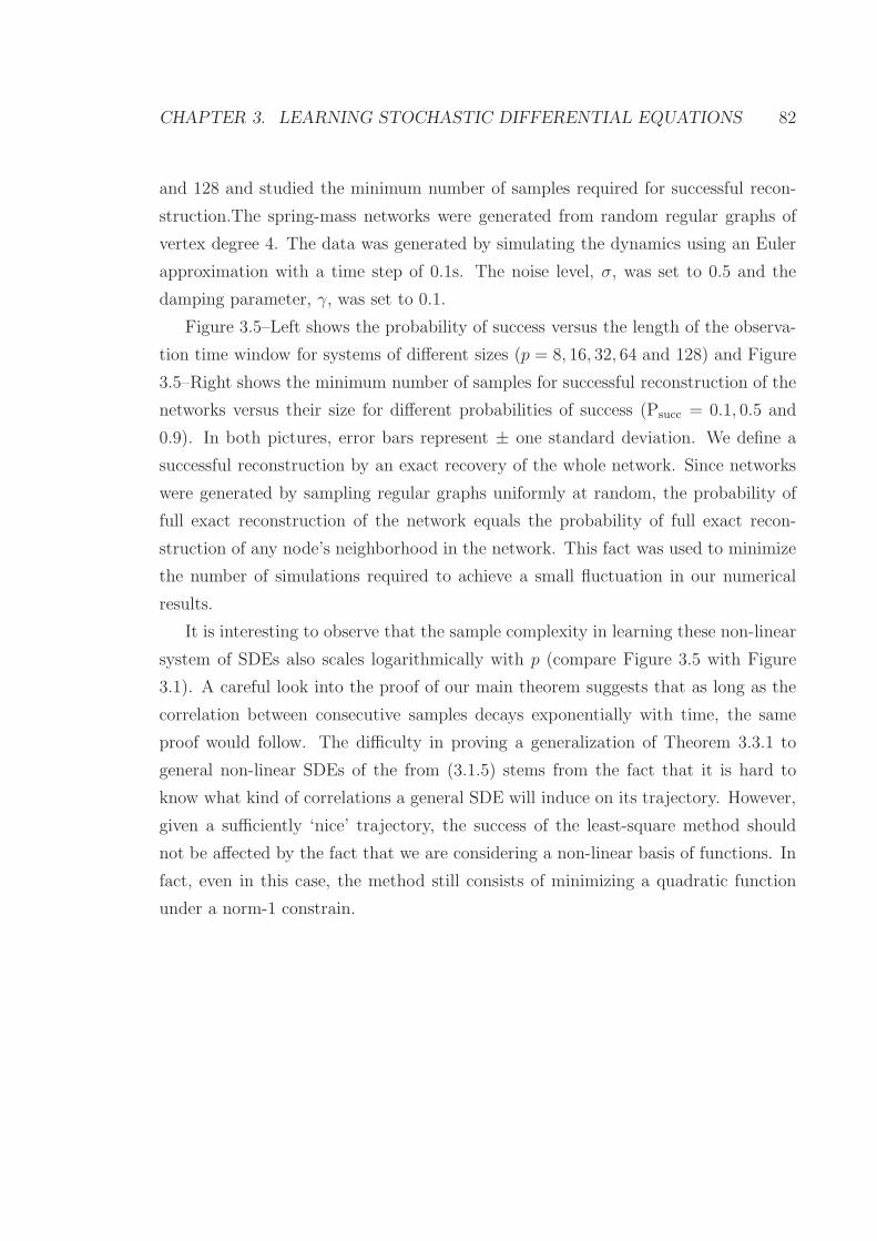
CHAPTER 3. LEARNING STOCHASTIC DIFFERENTIAL EQUATIONS 82
and 128 and studied the minimum number of samples required for successful recon-
struction.The spring-mass networks were generated from random regular graphs of
vertex degree 4. The data was generated by simulating the dynamics using an Euler
approximation with a time step of 0.1s. The noise level, σ, was set to 0.5 and the
damping parameter, γ, was set to 0.1.
Figure 3.5–Left shows the probability of success versus the length of the observa-
tion time window for systems of different sizes (p = 8, 16, 32, 64 and 128) and Figure
3.5–Right shows the minimum number of samples for successful reconstruction of the
networks versus their size for different probabilities of success (Psucc = 0.1, 0.5 and
0.9). In both pictures, error bars represent ± one standard deviation. We define a
successful reconstruction by an exact recovery of the whole network. Since networks
were generated by sampling regular graphs uniformly at random, the probability of
full exact reconstruction of the network equals the probability of full exact recon-
struction of any node’s neighborhood in the network. This fact was used to minimize
the number of simulations required to achieve a small fluctuation in our numerical
results.
It is interesting to observe that the sample complexity in learning these non-linear
system of SDEs also scales logarithmically with p (compare Figure 3.5 with Figure
3.1). A careful look into the proof of our main theorem suggests that as long as the
correlation between consecutive samples decays exponentially with time, the same
proof would follow. The difficulty in proving a generalization of Theorem 3.3.1 to
general non-linear SDEs of the from (3.1.5) stems from the fact that it is hard to
know what kind of correlations a general SDE will induce on its trajectory. However,
given a sufficiently ‘nice’ trajectory, the success of the least-square method should
not be affected by the fact that we are considering a non-linear basis of functions. In
fact, even in this case, the method still consists of minimizing a quadratic function
under a norm-1 constrain.

CHAPTER 3. LEARNING STOCHASTIC DIFFERENTIAL EQUATIONS 83
0 25 50 75 100 125 150 175 200 225 250 275 300
0
0.1
0.2
0.3
0.4
0.5
0.6
0.7
0.8
0.9
1
T
Pro
babi
lity
of s
ucce
ss
p = 8p = 16p = 32p = 64p = 128
2^3 2^4 2^5 2^6 2^7
0
25
50
75
100
125
150
175
200
225
250
p
Min
. # s
ampl
es fo
r su
cces
s pr
ob. =
0.1
, 0.5
, 0.9
Psucc
= 0.1
Psucc
= 0.5
Psucc
= 0.9
Figure 3.5: (left) Probability of success versus length of observation time window, T ,for different network sizes (p = 8, 16, 32, 64 and 128). (right) Minimum number ofsamples required to achieve a probability of reconstruction of Psucc = 0.1, 0.5 and 0.9versus the size of the network p. All networks where generated from random regulargraphs of degree 4 sampled uniformly at random. The dynamics’ parameters were setto σ = 0.5 and γ = 0.1
3.8.2 Biochemical pathway
As another example, we look at a biochemical pathway describing a general response
of a cell to a change in its environment. This change can be, for instance, a lesion on
the skin. The lesion causes some cells to generate diffusible ligands (L). These ligands
come upon receptors (R) on the cell membrane, which act like antennas. Receptors
that have caught a ligand can then be modified (phosphorylated ∗) by enzymes called
kinases (K). These modifications enable interactions with other substrates (S) which
eventually turn on the genetic program of platelets to move towards the source of
the injury. This sequence of events is what is called the chemical pathway and can
be thought of as a sequence of chemical reactions describing the interaction between
difference species inside and outside the cell. The general pathway in consideration is
described in [6] and reproduced bellow for completeness. Below, kf and kr describe
forward and backward rates of reaction. Expressions inside parenthesis, e.g. (LR∗),
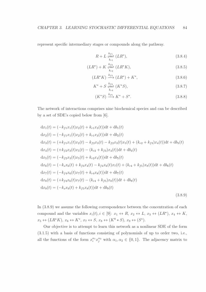
CHAPTER 3. LEARNING STOCHASTIC DIFFERENTIAL EQUATIONS 84
represent specific intermediary stages or compounds along the pathway.
R + Lkf1−−−−kr1
(LR∗), (3.8.4)
(LR∗) +Kkf2−−−−kr2
(LR∗K), (3.8.5)
(LR∗K)kf3−−→ (LR∗) +K∗, (3.8.6)
K∗ + Skf4−−−−kr4
(K∗S), (3.8.7)
(K∗S)kf5−−→ K∗ + S∗. (3.8.8)
The network of interactions comprises nine biochemical species and can be described
by a set of SDE’s copied below from [6].
dx1(t) = (−kf1x1(t)x2(t) + kr1x3(t))dt+ db1(t)
dx2(t) = (−kf1x1(t)x2(t) + kr1x3(t))dt+ db2(t)
dx3(t) = (+kf1x1(t)x2(t)− kf2x3(t)− kf2x3(t)x5(t) + (kr2 + kf3)x4(t))dt+ db3(t)
dx4(t) = (+kf2x3(t)x5(t)− (kr2 + kf3)x4(t))dt + db4(t)
dx5(t) = (−kf2x3(t)x5(t) + kr2x4(t))dt+ db5(t)
dx6(t) = (−ksx6(t) + kf3x4(t)− kf4x6(t)x7(t) + (kr4 + kf5)x8(t))dt + db6(t)
dx7(t) = (−kf4x6(t)x7(t) + kr4x8(t))dt+ db7(t)
dx8(t) = (+kf4x6(t)x7(t)− (kr4 + kf5)x8(t))dt + db8(t)
dx9(t) = (−ksx9(t) + kf5x8(t))dt + db9(t)
(3.8.9)
In (3.8.9) we assume the following correspondence between the concentration of each
compound and the variables xi(t), i ∈ [9]: x1 ↔ R, x2 ↔ L, x3 ↔ (LR∗), x4 ↔ K,
x5 ↔ (LR∗K), x6 ↔ K∗, x7 ↔ S, x8 ↔ (K8 ∗ S), x9 ↔ (S∗).
Our objective is to attempt to learn this network as a nonlinear SDE of the form
(3.1.5) with a basis of functions consisting of polynomials of up to order two, i.e.,
all the functions of the form xα1i xα2
j with α1, α2 ∈ 0, 1. The adjacency matrix to

CHAPTER 3. LEARNING STOCHASTIC DIFFERENTIAL EQUATIONS 85
be learned is Θ0 ∈ R9×46 which translates into approximately 400 parameters to be
estimated. We simulate the system in (3.8.9) using the Euler-Maruyama method to
obtain sample trajectories. We repeat the experiment 10 times, sampling independent
traces of the SDE’s trajectory. We obtain the following curves. Error bars represent
plus-minus one (empirical) standard deviation.
Figure 3.6 shows the true and false positive rates in reconstructing the support of
matrix Θ0.
Truepostive
rate
λ
10−1 100 101 102 1030.2
0.3
0.4
0.5
0.6
0.7
0.8
0.9
False
positiverate
λ
10−1 100 101 102 103
0.05
0.1
0.15
0.2
0.25
0.3
0.35
0.4
0.45
0.5
Figure 3.6: (left) True positive rate (right) false positive rate vs. λ for the durationof observation T = 1200.
Figure 3.7 shows the corresponding true positive rate versus false positive rate
curve (ROC curve) for different values of observation length T . The area under the
ROC curve is shown on the right plot in this figure. This value is an approximation
of the probability of choosing a random existing edge over a random non-existing
negative.
Finally, Fig. 3.8 shows the normalized root mean squared error (RMSE) defined
as
NRMSE ≡ ‖Θ0 − Θ‖2‖Θ0‖2
. (3.8.10)
The left plot shows the NRMSE versus λ. There exist an optimal value for the
parameter λ that minimized NRMSE. The right plot depicts NRMSE at the optimum
value of the parameter λ versus the length of the observation interval. NRMSE

CHAPTER 3. LEARNING STOCHASTIC DIFFERENTIAL EQUATIONS 86
T = 3000
T = 150
Tru
epositiverate
False positive rate0 0.2 0.4 0.6 0.8 1
0
0.1
0.2
0.3
0.4
0.5
0.6
0.7
0.8
0.9
1
Observation length500 1000 1500 2000 2500 3000
0.86
0.88
0.9
0.92
0.94
0.96
0.98
1.00
1.02
1.04
1.06
Figure 3.7: (left) ROC curves for different values of T . (right) Area under the ROCcurve vs. T .
drops below one as the observation length increases suggesting that the algorithm is
succeeding in reconstructing the signed support of the adjacency matrix Θ0.
NRMSE
λ
10−1 100 101 102 103
1
1.05
1.1
1.15
1.2
1.25
1.3
1.35
1.4
Observation time500 1000 1500 2000 2500 3000
0.89
0.9
0.91
0.92
0.93
0.94
0.95
0.96
0.97
0.98
0.99
Figure 3.8: (left) NRMSE vs. λ; T = 1200. (right) NRMSE vs. T for the optimumvalue of λ.

Appendix A
Learning the Ising model
A.1 Simple Thresholding
In the following we let Cij ≡ EG,θXiXj where expectation is taken with respect to
the Ising model (2.1.1).
Proof. (Theorem 2.3.1 ) If G is a tree then Cij = tanh θ for all (ij) ∈ E and Cij ≤tanh2 θ for all (ij) /∈ E. To see this notice that only paths that connect i to j
contribute to Cij and given that G is a tree there is only one such path and its length
is exactly 1 if (i, j) ∈ E and at least 2 when (i, j) /∈ E. The probability that Thr(τ)
fails is
1− Psucc = Pn,G,θCij < τ for some (i, j) ∈ E or Cij ≥ τ for some (i, j) /∈ E .(A.1.1)
Let τ = (tanh θ+tanh2 θ)/2. Applying Azuma-Hoeffding inequality to Cij =1n
∑nℓ=1 x
(ℓ)i x
(ℓ)j
we have that if (i, j) ∈ E then,
Pn,G,θ(Cij < τ) = Pn,G,θ
(n∑
ℓ=1
(x(ℓ)i x
(ℓ)j − Cij) < n(τ − tanh θ)
)≤ e−
132
n(tanh θ−tanh2 θ)2
(A.1.2)
87

APPENDIX A. LEARNING THE ISING MODEL 88
and if (i, j) /∈ E then similarly,
Pn,G,θ(Cij ≥ τ) = Pn,G,θ
(n∑
ℓ=1
(x(ℓ)i x
(ℓ)j − Cij) ≥ n(τ − tanh2 θ)
)≤ e−
132
n(tanh θ−tanh2 θ)2 .
(A.1.3)
Applying union bound over the two possibilities, (i, j) ∈ E or (i, j) /∈ E, and over the
edges (|E| < p2/2), we can bound Psucc by
Psucc ≥ 1− p2 e−132
n(tanh θ−tanh2 θ)2 . (A.1.4)
Imposing the right hand side to be larger than δ proves our result.
Proof. (Theorem 2.3.2) We will prove that, for θ < arctanh(1/(2∆)), Cij ≥ tanh θ
for all (i, j) ∈ E and Cij ≤ 1/(2∆) for all (ij) /∈ E. In particular Cij < Ckl for all
(i, j) /∈ E and all (k, l) ∈ E . The theorem follows from this fact via union bound
and Azuma-Hoeffding inequality as in the proof of Theorem 2.3.1.
The bound Cij ≥ tanh θ for (ij) ∈ E is a direct consequence of Griffiths inequality
[55] : compare the expectation of xixj in G with the same expectation in the graph
that only includes edge (i, j).
The second bound is derived using the technique of [40], i.e., bound Cij by the
generating function for self-avoiding walks on the graphs from i to j. More precisely,
assume l = dist(i, j) and denote by Nij(k) the number of self avoiding walks of length
k between i and j on G. Then [40] proves that
Cij ≤∞∑
k=l
(tanh θ)kNij(k) ≤∞∑
n=l
∆k−1(tanh θ)k ≤ ∆l−1(tanh θ)l
1−∆tanh θ≤ ∆(tanh θ)2
1−∆tanh θ.(A.1.5)
If θ < arctanh(1/(2∆)) the above implies Cij ≤ 1/(2∆) which is our claim.
Proof. (Theorem 2.3.3) The theorem is proved by constructing G as follows: sample a
uniformly random regular graph of degree ∆ over the p−2 vertices 1, 2, . . . , p−2 ≡[p − 2]. Add an extra edge between nodes p − 1 and p. The resulting graph is
not connected. We claim that for θ > K/∆ and with probability converging to 1

APPENDIX A. LEARNING THE ISING MODEL 89
as p → ∞, there exist i, j ∈ [p − 2] such that (i, j) /∈ E and Cij > Cp−1,p. As a
consequence, thresholding fails.
Obviously Cp−1,p = tanh θ. Choose i ∈ [p − 2] uniformly at random, and j a
node at a fixed distance t from i. We can compute Cij as p → ∞ using the same
local weak convergence result as in the proof of Lemma ??. Namely, Cij converges to
the correlation between the root and a leaf node in the tree Ising model (A.5.1). In
particular one can show, [83], that
limp→∞
Cij ≥ m(θ)2 , (A.1.6)
wherem(θ) = tanh(∆h0/(∆−1)) and h0 is the unique positive solution of Eq. (A.5.2).
The proof is completed by showing that tanh θ < m(θ)2 for all θ > K/∆.
A.2 Incoherence is a necessary condition: Proof of
Lemma 2.6.1
This proof follows closely the proof of Proposition 1 in [94]. For a matter of clarity
of exposition we include all the steps, even if these do not differ from the exposition
done in [94].
Here we show that, under the assumptions of the Lemma on the incoherence
condition, on σmin(Q0SS) and on λ, the probability that Rlr(λ) returns a θ satisfying θ =
(θS, θSC ) = (θS, 0) with θS > 0 is upper bounded as in Eq. (2.6.5). More specifically,
we will show that this θ will not satisfy the stationarity condition ∇Ln(θ) + λz = 0
with high probability for any sub-gradient z of the function ‖θ‖1 at θ.
To simplify notation we omit x(ℓ) in all the expressions involving and derived
from Ln.
Assume the event ∇Ln(θ) + λz = 0 holds for some θ as specified above. An
application of the mean value theorem yields
∇2Ln(θ0)[θ − θ0] = W n − λz − Rn , (A.2.1)

APPENDIX A. LEARNING THE ISING MODEL 90
where we recall W n = −∇Ln(θ0) and [Rn]j = [∇2Ln(θ(j))−∇2Ln(θ0)]∗j(θ − θ0) with
θ(j)
a point in the line from θ to θ0. Notice that by definition ∇2Ln(θ0) = Qn0 =
Qn(θ0). To simplify notation we omit the 0 in all Qn0. All Qn in this proof are thus
evaluated at θ0.
Breaking this expression into its S and SC components and since θSC = θ0SC = 0
we can write
QnSCS(θS − θ0S) = W n
SC − λzSC +RnSC , (A.2.2)
QnSS(θS − θ0S) = W n
S − λzS +RnS. (A.2.3)
Eliminating θS − θ0S from the two expressions we obtain
[W nSC −Rn
SC ]−QnSCS(Q
nSS)
−1[W nS −Rn
S] + λQnSCS(Q
nSS)
−1zS = λzSC . (A.2.4)
Now notice that QnSCS(Q
nSS)
−1 = T1 + T2 + T3 + T4 where
T1 = Q0SCS[(Q
nSS)
−1 − (Q0SS)
−1] , T2 = [QnSCS −Q0
SCS]Q0SS
−1,
T3 = [QnSCS −Q0
SCS][(QnSS)
−1 − (Q0SS)
−1] , T4 = Q0SCSQ
0SS
−1.
Recalling that zS = 1 and using the above decomposition we can lower bound the
absolute value of the indexed-i component of zSC by
|zi| ≥ ‖[Q0SCSQ
0SS
−1zS]i‖∞ − ‖T1,i‖1 − ‖T2,i‖1 − ‖T3,i‖1 (A.2.5)
−∣∣∣W
ni
λ
∣∣∣−∣∣∣R
ni
λ
∣∣∣− ‖[QnSCS(Q
nSS)
−1]i‖(∥∥∥W
nS
λ
∥∥∥∞+∥∥∥R
nS
λ
∥∥∥∞
).
We now assume that the samples x(ℓ) are such that the following event holds (notice
that i ∈ SC),
Ei ≡‖Qn
S∪i S −Q0S∪i S‖∞ < ξA,
∥∥∥W n
S∪iλ
∥∥∥∞
< ξB
, (A.2.6)
where ξA ≡ C2minǫ/(8∆) and ξB ≡ Cminǫ/(16
√∆).
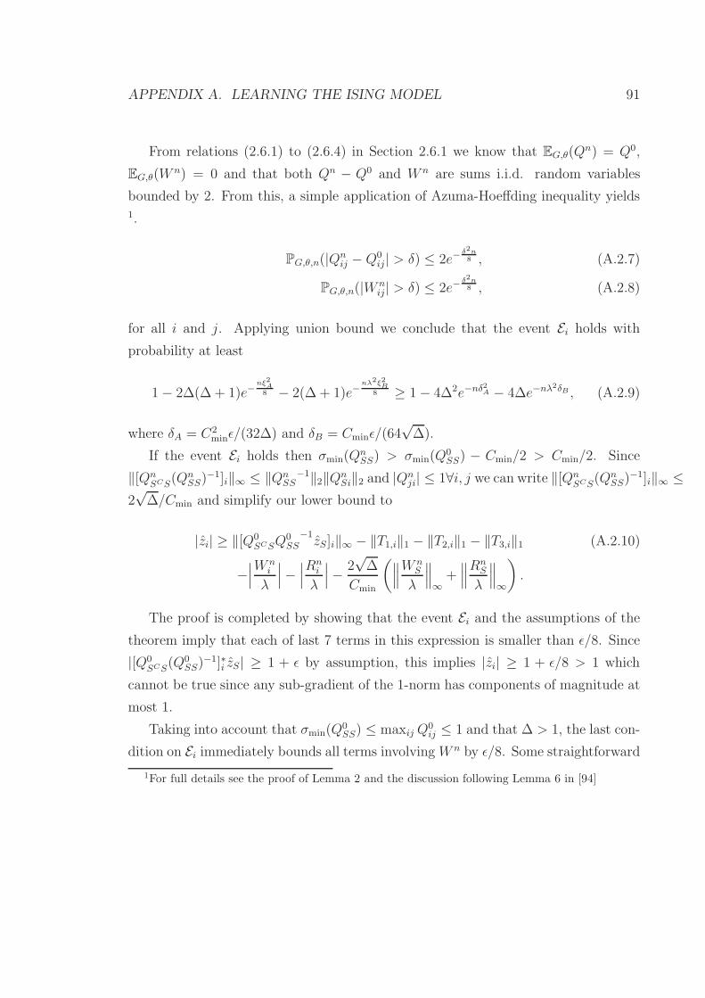
APPENDIX A. LEARNING THE ISING MODEL 91
From relations (2.6.1) to (2.6.4) in Section 2.6.1 we know that EG,θ(Qn) = Q0,
EG,θ(Wn) = 0 and that both Qn − Q0 and W n are sums i.i.d. random variables
bounded by 2. From this, a simple application of Azuma-Hoeffding inequality yields1.
PG,θ,n(|Qnij −Q0
ij | > δ) ≤ 2e−δ2n8 , (A.2.7)
PG,θ,n(|W nij| > δ) ≤ 2e−
δ2n8 , (A.2.8)
for all i and j. Applying union bound we conclude that the event Ei holds with
probability at least
1− 2∆(∆ + 1)e−nξ2A8 − 2(∆ + 1)e−
nλ2ξ2B8 ≥ 1− 4∆2e−nδ2A − 4∆e−nλ2δB , (A.2.9)
where δA = C2minǫ/(32∆) and δB = Cminǫ/(64
√∆).
If the event Ei holds then σmin(QnSS) > σmin(Q
0SS) − Cmin/2 > Cmin/2. Since
‖[QnSCS(Q
nSS)
−1]i‖∞ ≤ ‖QnSS
−1‖2‖QnSi‖2 and |Qn
ji| ≤ 1∀i, j we can write ‖[QnSCS(Q
nSS)
−1]i‖∞ ≤2√∆/Cmin and simplify our lower bound to
|zi| ≥ ‖[Q0SCSQ
0SS
−1zS]i‖∞ − ‖T1,i‖1 − ‖T2,i‖1 − ‖T3,i‖1 (A.2.10)
−∣∣∣W
ni
λ
∣∣∣−∣∣∣R
ni
λ
∣∣∣− 2√∆
Cmin
(∥∥∥WnS
λ
∥∥∥∞+∥∥∥R
nS
λ
∥∥∥∞
).
The proof is completed by showing that the event Ei and the assumptions of the
theorem imply that each of last 7 terms in this expression is smaller than ǫ/8. Since
|[Q0SCS(Q
0SS)
−1]∗i zS| ≥ 1 + ǫ by assumption, this implies |zi| ≥ 1 + ǫ/8 > 1 which
cannot be true since any sub-gradient of the 1-norm has components of magnitude at
most 1.
Taking into account that σmin(Q0SS) ≤ maxij Q
0ij ≤ 1 and that ∆ > 1, the last con-
dition on Ei immediately bounds all terms involving W n by ǫ/8. Some straightforward
1For full details see the proof of Lemma 2 and the discussion following Lemma 6 in [94]

APPENDIX A. LEARNING THE ISING MODEL 92
manipulations imply (see Lemma 7 from [94] for a similar computation)
‖T1,i‖1 ≤∆
C2min
‖QnSS −Q0
SS‖∞ , ‖T2,i‖1 ≤√∆
Cmin‖[Qn
SCS −Q0SCS]i‖∞ ,
‖T3,i‖1 ≤2∆
C2min
‖QnSS −Q0
SS‖∞‖[QnSCS −Q0
SCS]i‖∞ ,
and thus, again making use of the fact that σmin(Q0SS) ≤ 1, all will be bounded by
ǫ/8 when Ei holds. The final step of the proof consists in showing that if Ei holds andλ satisfies the condition given in the Lemma enunciation then the terms involving Rn
will also be bounded above by ǫ/8. The details of this calculation can be found in
[16].
A.3 Proof of Theorem 2.3.6: θ∆ ≤ 3/10
Before we prove the first part of Theorem 2.3.6 we need an auxiliary step to bound the
covariance Cij ≡ EG,θ(XiXj) between any two variables i, j ∈ V in our model (2.1.1).
This bound is derived using the technique of [40], i.e., bound Cij by the generating
function for self-avoiding walks on the graphs from i to j.
Lemma A.3.1. Assume l = dist(i, j) is the distance between node i and j in G and
denote by Nij(k) the number of self avoiding walks of length k between i and j on G.
Then [40] proves that
Cij ≤∞∑
k=l
(tanh θ)kNij(k) ≤∞∑
n=l
∆k−1(tanh θ)k (A.3.1)
≤ ∆l−1(tanh θ)l
1−∆tanh θ≤ ∆(tanh θ)2
1−∆tanh θ. (A.3.2)
The proof of the first part of our main theorem consists in showing that, in the
regime when θ∆ ≤ 3/10, all conditions of Theorem 1 in [94] (denoted there by A1
and A2) hold. In the process of verifying these conditions, we get explicit bounds for
several constants that remain unspecified in [94]. With this, we are able obtain our
bound on the sample complexity.

APPENDIX A. LEARNING THE ISING MODEL 93
In this proof all the functions are assumed to be evaluated at the true value of
the parameters θ0. Hence, throughout this proof, and to simplify notation, we denote
Qn0 = Qn(θ0) simply by Qn and W n0 = W n(θ0) by W n. In what follows, Cmin is a
lower bound for σmin(Q0SS) and Dmax
2 is an upper bound for σmax(Eθ(XSX∗S)). We
define 1−α ≡ ‖Q0SCS(Q
0SS)
−1‖∞ and let θmin denote the minimum absolute value of the
components of θ0. In our case we have θmin = θ. Throughout this proof we also have
Cmin ≡ σmin(QnSS), Dmax ≡ σmax
(1n
∑nl=1 x
(l)S x(l)∗
S
)and 1− α ≡ ‖Qn
SCS(QnSS)
−1‖∞.
We begin by noting that Theorem 1 in [94] can be rewritten in the following form,
Theorem A.3.1. If 0 < α < 1 and the events E and A hold true, then Rlr will not
fail.
The event E consists of the following conditions 3,
In Lemma 5,[94]: ‖QnSS −Q0
SS‖2 <Cmin
2, (A.3.3)
In Lemma 6,[94]: for T1 σmin(QnSS) ≥
Cmin
2, (A.3.4)
for T1 ‖QnSS −Q0
SS‖∞ ≤ 1
12
α
1− α
Cmin√∆
, (A.3.5)
for T2 ‖QnSCS −Q0
SCS‖∞ ≤ α
6
Cmin√∆
, (A.3.6)
for T3 ‖QnSCS −Q0
SCS‖∞ ≤√
α
6, (A.3.7)
In Lemma 7,[94]: σmin(QnSS) ≥
Cmin
2and (A.3.8)
‖QnSS −Q0
SS‖2 ≤√
α
6
C2min
2√∆
, (A.3.9)
In Proposition 1,[94]:‖W n‖∞
λ<
α
4(2− α). (A.3.10)
2It is easy to prove that Cmin ≤ Dmax
3These conditions are the conditions required for Theorem 1 in [94] to be applicable and arelabeled by the names of the intermediary results in [94] required to prove Theorem 1 in [94]

APPENDIX A. LEARNING THE ISING MODEL 94
The event A consists of the following bounds on the value of λ in Rlr(λ),
In Lemma 3,[94]: λ∆ ≤ C2min
10Dmax
, (A.3.11)
In Proposition 3,[94]:5
Cmin
λ√∆ ≤ θmin
2. (A.3.12)
Ravikumar et al. [94] show that the condition from Lemma 5 together with the
definition of Cmin and Dmax implies that Cmin ≥ Cmin/2 and Dmax ≤ 2Dmax. In
addition, the proof of Lemma 6 in [94] shows that, if (A.3.4) to (A.3.7) hold, then,
without loss of generality, we can assume α = α/2. This allows us to rewrite the right
hand side of all the above inequalities with constants only and no random variables
(remember that α, Dmax and Cmin are random variables). We call the new events
involving only constants on the right hand side by E ′ ⊆ E and A′ ⊆ A respectively.
Having the definition of E ′ and A′ in mind, Theorem 1 in [94] can be rewritten in
the following form,
Theorem A.3.2. If 1− α < 1 and the events A′ and E ′ hold true, then Rlr will not
fail.
The event E ′ consists of deviations of random vectors and matrices, under dif-
ferent norms, to their corresponding expected values. A straightforward application
of Azuma’s inequality yields the following upper bound on the probability of these
assumptions not occurring together 4,
Pn,G,θ(E ′c) ≤ 2e−n 132∆2 (d
(2)SS)
2+2 log∆ + 2e−n 132∆2 (d
(∞)SS )2+2 log∆ (A.3.13)
+ 2e−n 132∆2 (d
(∞)
SCS)2+log∆+log p−∆ + 2e−nλ2
27( α4−α
)2+log p ,
4The first three terms are for the conditions involving matrix Qn and the fourth with the eventdealing with matrix Wn

APPENDIX A. LEARNING THE ISING MODEL 95
where
d(2)SS = min
Cmin
2,
√α
6
C2min
2√∆
, (A.3.14)
d(∞)SS =
1
12
α
1− α
Cmin√∆
, (A.3.15)
d(∞)
SCS= min
α6
Cmin√∆
,
√α
6
. (A.3.16)
We want this probability to be upper bounded by δ/p. If this is the case, an appli-
cation of union bound allows to conclude that Rlr correctly recovers the neighborhood
of every node, and hence the whole graph G, with probability greater then 1− δ.
In the regime where θ∆ ≤ 3/10, we now compute explicit bounds for Cmin, Dmax
and α. Replacing them in (A.3.13) we simplify expression (A.3.13). Finally, from
this expression, we prove that the λ chosen in our main theorem suffices to obtain
the sample complexity stated.
In what follows we let K1 = 3/10. Also, recall that tanh x ≤ x for all x ≥ 0.
First notice that by (2.6.2) we have Cmin = σminEG,θ((1− tanh2 θM)XSX∗S) where
M =∑
t∈∂r Xt. Since θM ≤ θ∆ ≤ K1 we have, Cmin ≥ (1−K21 )σmin(EG,θXSX
∗S).
Now write EG,θXSX∗S ≡ I + T and notice that by (A.3.2) in Lemma A.3.1, T
is a symmetric matrix whose entries are non-negative and smaller than tanh θ/(1 −∆tanh θ). Since σmin(EG,θXSX
∗S) = 1 − v∗(−T )v for some unit norm vector v
and since, by Cauchy–Schwarz inequality, we have v∗(−T )v ≤ ‖v‖21maxij |Qij| ≤∆tanh θ/(1 − ∆tanh θ) ≤ K1/(1 − K1), it follows that σmin(EG,θXSX
∗S) ≥ (1 −
2K1)/(1 −K1). Consequently, Cmin ≥ (1 +K1)(1 − 2K1) = 13/25. Again using the
bound (A.3.2), we can write Dmax ≤ 1+∆ tanh θ/(1−∆tanh θ) ≤ (1−K1)−1 = 10/7.
Finally, we bound ‖Q0SCS(Q
0SS)
−1‖∞.
Before proceeding however, we need the follow technical Lemma.
Lemma A.3.2. If θ > 0, i ∈ S and j ∈ SC then,
Q0ij = EG,θ(1− tanh2(θM))XiXj ≤ EG,θ1− tanh2(θM)EG,θXiXj. (A.3.17)
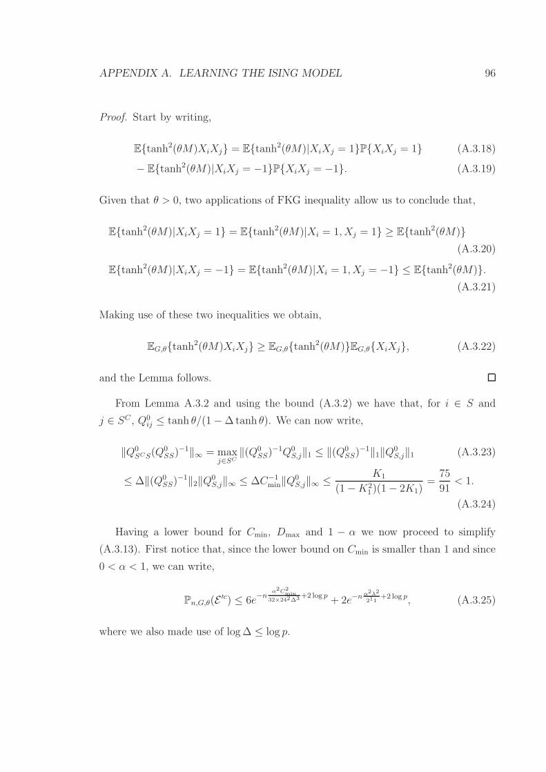
APPENDIX A. LEARNING THE ISING MODEL 96
Proof. Start by writing,
Etanh2(θM)XiXj = Etanh2(θM)|XiXj = 1PXiXj = 1 (A.3.18)
− Etanh2(θM)|XiXj = −1PXiXj = −1. (A.3.19)
Given that θ > 0, two applications of FKG inequality allow us to conclude that,
Etanh2(θM)|XiXj = 1 = Etanh2(θM)|Xi = 1, Xj = 1 ≥ Etanh2(θM)(A.3.20)
Etanh2(θM)|XiXj = −1 = Etanh2(θM)|Xi = 1, Xj = −1 ≤ Etanh2(θM).(A.3.21)
Making use of these two inequalities we obtain,
EG,θtanh2(θM)XiXj ≥ EG,θtanh2(θM)EG,θXiXj, (A.3.22)
and the Lemma follows.
From Lemma A.3.2 and using the bound (A.3.2) we have that, for i ∈ S and
j ∈ SC , Q0ij ≤ tanh θ/(1−∆tanh θ). We can now write,
‖Q0SCS(Q
0SS)
−1‖∞ = maxj∈SC
‖(Q0SS)
−1Q0S,j‖1 ≤ ‖(Q0
SS)−1‖1‖Q0
S,j‖1 (A.3.23)
≤ ∆‖(Q0SS)
−1‖2‖Q0S,j‖∞ ≤ ∆C−1
min‖Q0S,j‖∞ ≤ K1
(1−K21 )(1− 2K1)
=75
91< 1.
(A.3.24)
Having a lower bound for Cmin, Dmax and 1 − α we now proceed to simplify
(A.3.13). First notice that, since the lower bound on Cmin is smaller than 1 and since
0 < α < 1, we can write,
Pn,G,θ(E ′c) ≤ 6e−n
α2C2min
32×242∆3+2 log p+ 2e−nα2λ2
211+2 log p, (A.3.25)
where we also made use of log∆ ≤ log p.

APPENDIX A. LEARNING THE ISING MODEL 97
Bounding the first term by (3δ)/(4p) and the second term by δ/(4p) is enough to
guarantee that the probability of full reconstruction of G is greater then 1−δ. Taking
into account the values of the bounds for α and Cmin, we conclude that
n > 32× 242∆3α−2C−2min log(8p
3/δ), (A.3.26)
suffices for the bound on the first term to hold. For the bound on the second term to
hold, it suffices that
nλ2 > 211α−2 log(8p3/δ). (A.3.27)
Now notice that event A′ imposes the following two conditions on λ,
λ ≤ C2min
80∆Dmax
, (A.3.28)
λ ≤ θCmin
20√∆. (A.3.29)
It is not hard to see that, for ∆ ≥ 3 and if θ∆ ≤ K1, the second condition on λ
implies the first one. Having this in mind one easily sees that, when λ ≤ 13θ500
√∆, the
second restriction on n (A.3.27) implies the first one (A.3.26). This proves the first
part of Theorem 2.3.6.
A.4 Graphs in Gdiam(p,∆): Proof of Lemma 2.6.3
Let us focus on reconstructing the neighborhood of node r = 1 in G ∈ Gdiam(p,∆). If
we cannot reconstruct this neighborhood then we also cannot reconstruct the graph
G correctly.
First notice that, by strong duality, the convex problem minθ∈Rp−1 Ln(θ) + λ‖θ‖1can be equivalently written as minθ∈Rp−1:‖θ‖1≤C Ln(θ) for some C = C(λ) > 0.
We denote any solution of these problem by θ(λ) and θ(C) respectively. Notice
also that λ ≥ λmin is equivalent to C ∈ [0, Cmax] for some Cmax = Cmax(∆, λmin).
Therefore, without loss of generality, we can assume that θ belongs to the compact
set ‖θ‖1 ≤ Cmax. Furthermore, notice that Ln(θ) = (1/n)∑n
ℓ=1 f(θ,X(ℓ)) where

APPENDIX A. LEARNING THE ISING MODEL 98
f(x, y) ≤ 2Cmax + log 2 and is Lipschitz in x for every y. Consequently, since X(ℓ)are i.i.d. random variables, this representation of Ln(.) guarantees that with proba-
bility one, Ln(θ) converges to L(θ) uniformly over ‖θ‖1 ≤ Cmax as n → ∞, [96].
Secondly, it is not hard to see that L(θ) is strictly convex. Hence the problem
minθ∈Rp−1:‖θ‖1≤C L(θ) has a unique solution. Call it θ∞(C) ∈ Rp−1. Because with
probability one, Ln(θ) converges to L(θ) uniformly over ‖θ‖ ≤ Cmax, and because
both L and Ln are continuous, we have that any θ(C) converges to θ∞(C) uniformly
over C ∈ [0, Cmax] as n → ∞.
Finally, as a consequence the equivalence between the two optimization problems
mentioned in the first paragraph, we have
supλ≥λmin
PG(λ) = G ≤ supC∈[0,Cmax]
Psupp(θ∞(C)) = ∂r. (A.4.1)
Consequently, if we prove that supp(θ∞(C)) 6= ∂r for all C ∈ [0, Cmax] then
supλ≥λmin
PG(λ) = G ≤ supC∈[0,Cmax]
Psupp(θ∞(C)) = ∂r → 0, as n → ∞ (A.4.2)
and therefore,
supλ≥λmin
PG(λ) = G ≤ ǫ, for all n ≥ n0(∆, ǫ, λmin), (A.4.3)
which would finish the proof.
In order to prove that supp(θ∞(C)) 6= ∂r first observe that by symmetry, the
unique solution θ∞ = θ∞12, θ∞13, ..., θ∞1p ∈ Rp−1 satisfies, θ∞13 = θ∞14, ..., θ
∞1p. Hence,
all we need to prove is that we cannot have θ∞12 = 0 and θ∞13 6= 0. To study these
two components of θ∞, we define L(θ13, θ12) = L(θ12, θ13, θ13, ..., θ13) and solve the
optimization problem
minθ13,θ12∈R
L(θ13, θ12) + λ∆|θ13|+ λ|θ13|. (A.4.4)
The following lemma now completes the proof.

APPENDIX A. LEARNING THE ISING MODEL 99
Lemma A.4.1. For ∆ ≥ 50, if 2 ≤ ∆θ ≤ 3 and λ > 0 then no solution of
minθ13,θ12
L(θ13, θ12) + λ∆|θ13|+ λ|θ13| (A.4.5)
simultaneously satisfies θ12 = 0 and θ13 6= 0.
Proof. Let L(θ13, θ12) = L(θ13, θ12) + λ∆|θ13|+ λ|θ13|. A solution of the convex opti-
mization problem (A.4.5) satisfies θ12 = 0 and θ13 6= 0 for some λ > 0 if and only if,
for some λ > 0, θ12 = 0 and θ13 6= 0 , we have
∂L∂θ12
∋ 0, (A.4.6)
∂L∂θ13
∋ 0. (A.4.7)
Above we use ‘∋ 0’ to signify that the sub-gradient of L must contain 0.
Let Z = X3 + ... +Xp and notice that
L(θ13, θ12) = log 2 + Elog cosh(Zθ13 +X2θ12) −∆θ13EX1X3 − θ12EX1X2.(A.4.8)
Since (log cosh x)′ = tanh x the above optimality conditions can be written as,
∂L∂θ12
∣∣∣∣θ12=0,θ13>0
= EX2 tanh(Zθ13) − EX1X2+ λ∂|θ12|∂θ12
∋ 0, (A.4.9)
∂L∂θ13
= EZ tanh(Zθ13) −∆EX1X3+ λ∆∂|θ13|∂θ13
(A.4.10)
= ∆EX3 tanh(Zθ13) −∆EX1X3+ λ∆∂|θ13|∂θ13
(A.4.11)
= ∆EX3 tanh(Zθ13) −∆EX1X3 ± λ∆ = 0, (A.4.12)
where in the last line we used the fact that, for θ13 6= 0 we have ∂|θ13|∂θ13
∈ −1, 1.From the last condition we conclude that λmust satisfy λ = EX1X3−EX3 tanh(Zθ13)
if θ13 > 0 or λ = −EX1X3 + EX3 tanh(Zθ13) if θ13 < 0. But by symme-
try EX3 tanh(Zθ13) = ∆−1EZ tanh(Zθ13) which is strictly negative if θ13 < 0.
Hence, not to contradict the fact that λ > 0, it must be that θ13 > 0 and λ =

APPENDIX A. LEARNING THE ISING MODEL 100
EX1X3 − EX3 tanh(Zθ13).From now on we assume that EX1X3−EX3 tanh(Zθ13) > 0, otherwise λ ≤ 0
and the proof again follows by contradiction. Replacing this value in the first condition
we obtain,∂|θ12|∂θ12
∋ EX1X2 − EX2 tanh(Zθ13)EX1X3 − EX3 tanh(Zθ13)
. (A.4.13)
The sub-gradient of the modulus function can only take values in [−1, 1]. To
finish the proof we now show that, under the conditions of Lemma A.4.1 and for any
θ13 > 0,
EX1X2 − EX2 tanh(Zθ13) − EX1X3+ EX3 tanh(Zθ13) > 0. (A.4.14)
This implies that the optimality conditions cannot be satisfied for any λ > 0 when
θ13 > 0 and θ12 = 0.
Let us define, β ≡ θ13 and
F (β) ≡ EX1X2 − EX2 tanh(Zβ) − EX1X3+ EX3 tanh(Zβ). (A.4.15)
Since PGp,θ(X1 = 1|X2, ..., Xp) = eθZ/(eθZ+e−θZ) we have that EX1|Z = EX2|Z =
tanh(Zθ). This allows us to make the following substitutions in (A.4.15),
EX1X2 = EX2 tanh(θZ), (A.4.16)
EX1X3 = EX3 tanh(θZ), (A.4.17)
EX2 tanh(Zβ) = Etanh(θZ) tanh(Zβ), (A.4.18)
and by symmetry, EX3 tanh(θZ) = ∆−1EZ tanh(θZ). With these substitutions,
and introducing Z = ∆−1Z, we obtain
F (β) = E(tanh(θ∆Z)− Z)(tanh(θ∆Z)− tanh(β∆Z)). (A.4.19)
Let us denote the expression inside the expectation byH(Z), that is, F (β) = EH(Z).
APPENDIX A. LEARNING THE ISING MODEL 101
Since H(Z) is an even function of Z we can write,
F (β) = 2EH(Z)IZ>0 = 2EH(Z)IZ>0,θ∆Z>γ+ 2EH(Z)IZ>0,θ∆Z≤γ. (A.4.20)
We now make use of the following inequalities
(1− tanh2 a)(a− b) ≤ tanh(a)− tanh(b) ≤ a− b, 0 ≤ a ≤ b, (A.4.21)
tanh(a) ≥ aγ−1 tanh γ, 0 ≤ a ≤ γ, (A.4.22)
to obtain a lower bound on F (β). First notice that,
2EH(Z)IZ>0,θ∆Z≤γ ≥ 2E(θ∆Z tanh γ
γ− Z
)(1− tanh2 γ)(θ − β)∆Z IZ>0,θ∆Z≤γ
(A.4.23)
= 2
(θ∆tanh γ
γ− 1
)(1− tanh2 γ)(θ − β)∆E
Z2 IZ>0,θ∆Z≤γ
(A.4.24)
=
(θ∆tanh γ
γ− 1
)(1− tanh2 γ)(θ − β)∆E
Z2 I|Z|≤ γ
∆θ
,
(A.4.25)
and also that,
2EH(Z)IZ>0,θ∆Z>γ ≥ −2E(1 − tanh(θ∆))(θ − β)∆Z IZ>0,θ∆Z>γ (A.4.26)
≥ −2(1 − tanh(θ∆))(θ − β)∆EIZ>0,θ∆Z>γ (A.4.27)
= −2(1− tanh(θ∆))(θ − β)∆PZ > 0, θ∆Z > γ (A.4.28)
= −(1− tanh(θ∆))(θ − β)∆P|Z| > γ
θ∆
. (A.4.29)
Since |Z| ≤ 1,
EZ2 I|Z|≤ γ
∆θ
≥ EZ2 − P
|Z| ≤ γ
∆θ
, (A.4.30)

APPENDIX A. LEARNING THE ISING MODEL 102
summing both expressions above and rearranging terms we obtain
F (β)
∆(θ − β)≥(θ∆tanh γ
γ− 1
)(1− tanh2 γ)EZ2 (A.4.31)
−((
θ∆tanh γ
γ− 1
)(1− tanh2 γ) + (1− tanh(θ∆))
)P|Z| > γ
θ∆
.
(A.4.32)
We now set γ = 1.64. Since ∆θ ≥ 2, a quick numerical calculation shows that(θ∆tanh γ
γ− 1)(1− tanh2 γ) > 3.3224(1− tanh(θ∆)) > 0 and hence,
F (β)
∆(θ − β)≥(θ∆tanh γ
γ− 1
)(1− tanh2 γ)
(EZ2 − 1.3010P
|Z| > γ
θ∆
).
(A.4.33)
We compute a value for EZ2 and then an upper bound for P|Z| > γ
θ∆
.
Using the fact that EXiXj = EX3X4 for all i 6= j, i, j /∈ 1, 2 we have
EZ2 = ∆−2EZ2 = ∆−2(∆ +∆(∆− 1)EX3X4) = ∆−1 + (∆− 1)∆−1EX3X4.(A.4.34)
For the probability bound, start by noticing that PX1 = X2 = 1 ≥ PX1 =
1, X2 = −1. Then we can write,
P|Z| > γ
θ∆
≤ 2
(P|Z| > γ
θ∆
∣∣∣X1 = X2 = 1+ P
|Z| > γ
θ∆
∣∣∣X1 = 1, X2 = −1)
(A.4.35)
× PX1 = X2 = 1. (A.4.36)
Conditioned on X1 = X2 = 1, the random variable Z is the average of i.i.d. random
variables that take values in −1, 1 and whose mean is tanh 2θ. Now we apply the
Chernoff-Hoeffding bound. Since ∆ ≥ 50 and θ∆ ≤ 3 we have γθ∆
− tanh(2θ) ≥
APPENDIX A. LEARNING THE ISING MODEL 103
1.64/3− tanh(2× 3/50) ≥ 0.4272 and we can write,
P|Z| > γ
θ∆
∣∣∣X1 = X2 = 1≤ 2P
Z >
γ
θ∆− tanh 2θ
∣∣∣X1 = X2 = 1
(A.4.37)
≤ 2e−12∆( γ
θ∆−tanh 2θ)
2
≤ 2e−0.09126∆. (A.4.38)
Conditioned on X1 = 1, X2 = −1, the random variable Z is the average of i.i.d.
random variables that take values in −1, 1 and whose mean is zero. Again using
the Chernoff-Hoeffding bound, and since γθ∆
≥ 1.64/3 we obtain,
P|Z| > γ
θ∆
∣∣∣X1 = 1, X2 = −1≤ 2e−
12∆( γ
θ∆)2
≤ 2e−0.1494∆. (A.4.39)
Putting these two last bounds together, we obtain
P|Z| > γ
θ∆
≤ 4e−0.09126∆PX1 = X2 = 1 = 4e−0.09126∆
(1 + EX1X2
4
).
(A.4.40)
In order to guarantee that F (β) > 0 it suffices that,
∆−1 > 1.3010e−12∆(tanh 2θ)2 , (A.4.41)
∆− 1
∆EX3X4 > 1.3010e−
12∆(tanh 2θ)2EX1X2. (A.4.42)
Since
EX1X2 = tanh(∆atanh((tanh θ)2)), (A.4.43)
EX3X4 = 2(tanh(2θ))2PX1 = X2 = 1 = 1/2(tanh(2θ))2(1 + EX1X2),(A.4.44)
we have EX3X4/EX1X2 ≥ 2/∆. In addition, since ∆ ≥ 50 we have (∆−1)/∆ ≥49/50 and hence it suffices that
∆−1 − 1.3010e−0.09126∆ > 0. (A.4.45)

APPENDIX A. LEARNING THE ISING MODEL 104
Figure A.1: For this family of graphs of increasing maximum degree ∆ Rlr(λ) will failfor any λ > 0 if θ ≥ 2/∆.
Since 1/50− 1.3010e−0.09126×50 = 0.006429 > 0 the proof now follows.
A.4.1 Graphs Gdiam(p) from the Section 2.6.3: Remark 2.3.1
and Remark 2.6.1
In Section A.4 we proved Lemma 2.6.3: Rlr(λ), λ > 0, fails to reconstruct graphs
from Gdiam(p) assymptotically (as n → ∞ with λ fixed) when 2 ≤ θ∆ ≤ 3. In this
section we numerically investigate the behavior of Rlr in more detail and numerically
demonstrate that in fact we do not need to impose that ∆θ ≤ 3 and that we can take
∆0 = 3.
As we saw in Section A.4, for large n, the success of Rlr is dictated by
minθ13,θ12∈R
L(θ13, θ12) + λ∆|θ13|+ λ|θ12| (A.4.46)
having an optimal solution with θ13 6= 0 and θ12 = 0.
Since it only involves two variables, we can easily analyze this optimization prob-
lem by solving it numerically. Figure A.2 shows the solution path of this problem as
a function of λ for p = 5 and for different values of θ.
From the plots we see that for high values of θ, Rlr will never yield a correct
reconstruction (unless we assume λ = 0) since for these θs the curves are strictly
above the horizontal (θ12 > 0) for all λ > 0. However, if θ is bellow a certain value,
call it θT (θT ≈ 0.61 for p = 5), then there are λ > 0 for which the solution yields a
correct reconstruction. In fact, for θ < θT all curves exhibit a portion (above a certain
λ) that have θ12 = 0 and θ13 > 0. In addition, we observe that there is a value θL
such that if θ < θL the curves identify themselves with the horizontal axis for all λ.

APPENDIX A. LEARNING THE ISING MODEL 105
θ = 0.51
θ = 0.55
θ = 0.65
θ = 0.61
λ = 0θ13 = θ
λ = ∞ θ13
θ12
Figure A.2: Solution curves of Rlr(λ) as a function of λ for different values of θ andp = 5. Along each curve, λ increases from right to left. Plot points separated byδλ = 0.05 are included to show the speed of the parameterization with λ. For λ → ∞all curves tend to the point (0, 0). For λ = 0, θ13 = θ. Remark: Curves like the onefor θ = 0.55 are identically zero above a certain value of λ.
APPENDIX A. LEARNING THE ISING MODEL 106
All the above observations hold in the limit when n → ∞. For high finite n,
with probability close to one (and uniformly over θ13, θ13 and λ – cf. Section A.4)
the solution curves will not be the ones plotted but rather be random fluctuations
around these. For λ = 0, finite n and θ > θL, the solution curves will no longer start
from θ = (θ13, θ13) = θ0 = (θ, 0) but will have a positive non vanishing probability of
having θ12 > 0. This reflects the fact that for finite n the success of Rlr(λ) requires
λ to be positive. However, for θ < θL and λ > 0 such that we are in the region
where the curves for n = ∞ are identically zero, the curves for finite n will have an
increasing probability of being identically zero too. Thus, for these values of λ and
θ, the probability of successful reconstruction will tend to 1 as n → ∞. From the
plots we also conclude that, unless the whole curve (for n = ∞) is identified with
zero, Rlr(λ) restricted to the assumption λ → 0 will fail with positive non vanishing
probability for finite n. For θ < θL, when the curves (for n = ∞) become identically
zero, there will be a scaling of λ with n to zero that will allow for a probability of
success converging to 1 as n → ∞.
When λ → 0 with n, θL is the critical value above which reconstruction with
Rlr fails. This is the related to the requirement that λ is small in Lemma 2.6.3. In
fact, θL coincides with the value above which ‖Q0SCS(Q
0SS)
−1z0S‖∞ > 1. However, we
do not have to choose λ → 0. We thus conclude that, for graphs in Gdiam(p), the
true condition required for successful reconstruction is not ‖Q0SCS(Q
0SS)
−1‖∞ < 1 but
rather that θ < θT . Surprisingly, for graphs in Gdiam(p), this condition coincides with
EG,θ(X1X3) > EG,θ(X1X2), i.e. the correlation between neighboring nodes must be
bigger than that between non-neighboring nodes.
This can be see in the following way. In the proof of Lemma 2.6.3 we proved that
the failure of Rlr(λ) for λ > 0 is equivalent to F (β) being positive for all 0 ≤ β < θ.
From equation (A.4.19) in the proof, we also know that F (θ) = 0. We now argue that
F also has the following property: θ is the smallest positive solution of F (β) = 0. A

APPENDIX A. LEARNING THE ISING MODEL 107
0.2 0.4 0.6 0.8 1.0
- 0.05
0.05
θ = 0.1
θ = 0.2θ = 0.6
θ = 0.5
θ = 0.3
θ = 0.4
β
F (β)
Figure A.3: F (β) for p = 6. Red θ = 0.1, 0.2, 0.3. Blue θ = 0.4, 0.5, 0.6.
brute force computation shows that F (β) can be written as,
F (β) =
(1
2
(tanh
((p− 2) tanh−1
(tanh2(θ)
))+ 1)− 1
)
×(
p−3∑
r=0
23−p
(p− 3
r
)tanh(β(−p+ 2r + 2)) + 1
)
−(1− e2θ
e−2θ + e2θ
)(tanh
((p− 2) tanh−1
(tanh2(θ)
))+ 1)
×(
p−3∑
r=0
(e2θ
e−2θ + e2θ
)r (p− 3
r
)(1− e2θ
e−2θ + e2θ
)p−r−3
tanh(β(−p+ 2r + 2))− 1
).
With this function we produced Figure A.3, where we plot F (β) for several values of
θ for p = 6 (similar plots are observed for other values of p ≥ 5). From the plots, one
observes that in fact, the smallest value of β > 0 for which F (β) = 0 corresponds to
β = θ. Because of this, F (0) > 0 if and only if F (β) > 0, ∀β ∈ [0, θ). Hence, the
asymptotic failure of Rlr(λ) for λ > 0 is equivalent to F (0) = EX1X2−EX1X3 >
0. Or in other words, the success is equivalent to EX1X3 > EX1X2.

APPENDIX A. LEARNING THE ISING MODEL 108
Remark A.4.1. Notice that this condition is also the condition required for the sim-
ple thresholding algorithm Thr(τ) to reconstruct a graph: the correlation between con-
nected nodes needs to be greater than the correlation between non-connected nodes.
We will now prove that if ∆ ≥ 3 and ∆θ ≥ 2 then EX1X2 > EX1X3.Let 1 and 2 be the two nodes with degree greater than 2 and let 3 be any other
node (of degree 2), see Figure A.1. Define x∆ = EG,θ(X1X2) and y∆ = EG,θ(X1X3).
It is not hard to see that,
x∆+1 =x∆ + tanh2 θ
1 + tanh2 θ x∆
y∆+1 =tanh θ x∆ + tanh θ
1 + tanh2 θ x∆
. (A.4.47)
From these expression we see that the condition x∆(θ) > y∆(θ) is equivalent to
x∆−1(θ) > tanh θ.
Since tanh(a + b) = tanh a+tanh b1+tanh a tanh b
, from the recursion for x∆ we can obtain
x∆−1 = tanh((∆− 1)arctanh(tanh2(θ))
). (A.4.48)
Therefore, x∆(θ) > y∆(θ) is equivalent to (∆− 1)arctanh(tanh2(θ)) > θ. But for θ >
0, θ > θ−1arctanh(tanh2(θ)). Hence, if (∆− 1)θ ≥ 1 we have EX1X2 > EX1X3.But (∆−1)θ ≥ 1 is equivalent to ∆θ ≥ ∆/(∆−1) and for ∆ ≥ 3, ∆/(∆−1) ≤ 3/2 ≤ 2
so our claim follows.
A.5 Graphs in Grand(p,∆): Proof of Lemma 2.6.4
To prove this theorem we will show that there exists θThr(∆) such that, when θ >
θThr(∆), we can compute constants ǫ = ǫ(∆, θ) and Cmin = Cmin(∆, θ) such that all
the conditions of Lemma 2.6.1 hold when we define λThr(∆, θ) = C3minǫ/(2
7(1+ǫ2)∆3).
First, let us state explicitly the local weak convergence result mentioned in Sec. ??
right after our statement of Lemma 2.6.4. For t ∈ N, let T(t) = (VT, ET) be the regular
rooted tree of degree ∆ of t generations and define the associated Ising measure as
µ+T,θ(x) =
1
ZT,θ
∏
(i,j)∈ET
eθxixj
∏
i∈∂T(t)eh
0xi . (A.5.1)

APPENDIX A. LEARNING THE ISING MODEL 109
Here ∂T(t) is the set of leaves of T(t) and h0 is the unique positive solution of
h = (∆− 1) atanh tanh θ tanhh . (A.5.2)
It was proved in [83] that non-trivial local expectations with respect to PG,θ(x) con-
verge to local expectations with respect to µ+T,θ(x), as p → ∞.
More precisely, let Br(t) denote a ball of radius t around node r ∈ G (the node
whose neighborhood we are trying to reconstruct). For any fixed t, the probability
that Br(t) is not isomorphic to T(t) goes to 0 as p → ∞.
Let g(xBr(t)) be any function of the variables in Br(t) such that g(xBr(t)) =
g(−xBr(t)). Then almost surely over graph sequences Gp of uniformly random regular
graphs with p nodes (expectations here are taken with respect to the measures (2.1.1)
and (A.5.1))
limp→∞
EG,θg(XBr(t)) = ET(t),θ,+g(XT(t)) . (A.5.3)
Notice that this characterizes expectations completely since if g(xBr(t)) = −g(−xBr(t))
then,
EG,θg(XBr(t)) = 0. (A.5.4)
The main part of the proof consists in considering [Q0SCSQ
0SS
−1z0S]i for t = dist(r, i)
bounded. We then write (Q0SS)lk = EG,θgl,k(X
Br(t)) and (Q0
SCS)il = EG,θgi,l(XBr(t)
)for some functions g·,·(X
Br(t)) and apply the weak convergence result (A.5.3) to these
expectations. We thus reduced the calculation of [Q0SCS(Q
0SS)
−1z0S]i to the calculation
of expectations with respect to the tree measure (A.5.1). The latter can be imple-
mented explicitly through a recursive procedure, with simplifications arising thanks
to the tree symmetry and by taking t ≫ 1. A similar computation is done with
regards to obtaining Cmin, the lower bound on σmin(Q0SS). The actual calculations
consist in a (very) long exercise in calculus and can be found in the appendix of [16].

Appendix B
Learning stochastic differential
equations
In this appendix we include all details of the proofs of Chapter 3. We start by
proving the upper bounds on the sample complexity and then proceed to prove the
lower bounds. Each of these proofs are included in a separate section. Auxiliary
lemmas are be introduced as needed and are proven in a separate subsection inside
sections.
B.1 Upper bounds on sample complexity of the
regularized least squares algorithm
Our result for the continuous time model follows from an analysis of the problem for
discrete time, introduced in Section 3.5.1, and taking the limit when η → 0. Hence,
we first prove Theorem 3.5.1, then we prove Theorem 3.3.1 and finally we prove the
specialization this bound to the case of the Laplacian of a graph, Theorem 3.3.4.
110

APPENDIX B. LEARNING STOCHASTIC DIFFERENTIAL EQUATIONS 111
B.2 Necessary condition for successful reconstruc-
tion of SDEs
In this Section we prove our main result for discrete-time dynamics, i.e., Theorem
3.5.1. We start by stating a set of sufficient conditions for regularized least squares
to work. Then we present a series of concentration lemmas to be used to prove the
validity of these conditions, and then finalize the proof.
As mentioned, the proof strategy, and in particular the following proposition,
Proposition B.2.1, which provides a compact set of sufficient conditions for the support
to be recovered correctly, is analogous to the one in [116]. A proof of this proposition
can be found in the end of this subsection.
In the following we denote by X ∈ Rp×n the matrix whose (t + 1)th column
corresponds to the configuration x(t), i.e. X = [x(0), x(1), . . . , x(n − 1)]. Further
∆X ∈ Rp×n is the matrix containing consecutive state changes, namely ∆X = [x(1)−
x(0), . . . , x(n) − x(n − 1)]. It is important not to confuse Xn0 ≡ x(t) : 0 ≤ t ≤ n
with X defined here. These are not the same. In addition, although both are related,
Xn0 should not be confused with the nth power of X (which is never mentioned in this
thesis). Finally we write W = [w(1), . . . , w(n− 1)] ∈ Rp×n for the matrix containing
the Gaussian noise realization. Equivalently,
W = ∆X − ηΘX .
The rth row of W is denoted by Wr.
In order to lighten the notation, we omit the reference to Xn0 in the likelihood
function (3.5.3) and simply write L(Θr). We define its normalized gradient and
Hessian by
G = −∇L(Θ0r) =
1
nηXW ∗
r , Q = ∇2L(Θ0r) =
1
nXX∗ . (B.2.1)
Proposition B.2.1. Let α,Cmin > 0 be be defined by
λmin(Q0S0,S0) ≡ Cmin , |||Q0
(S0)C ,S0
(Q0
S0,S0
)−1 |||∞ ≡ 1− α . (B.2.2)

APPENDIX B. LEARNING STOCHASTIC DIFFERENTIAL EQUATIONS 112
If the following conditions hold,
‖G‖∞ ≤ λα
3, ‖GS0‖∞ ≤ ΘminCmin
4∆− λ, (B.2.3)
|||Q(S0)C ,S0 −Q0(S0)C ,S0|||∞ ≤ α
12
Cmin√∆
, |||QS0,S0 −Q0S0,S0|||∞ ≤ α
12
Cmin√∆
, (B.2.4)
then the regularized least squares solution (3.5.2) correctly recovers sign(Θ0r). Further
the same statement holds for the continuous model 3.3.2, provided G and Q are the
gradient and the hessian of the likelihood (3.3.2).
The proof of Theorem 3.5.1 consists in checking that, under the hypothesis (3.5.6)
on the number of consecutive configurations, conditions (B.2.3) to (B.2.4) hold with
high probability. Checking these conditions can be regarded in turn as concentration-
of-measure statements. Indeed, if expectation is taken with respect to a stationary
trajectory, we have EG = 0, EQ = Q0.
The proof of B.2.1 can be bound in the appendix of [13].
In Section B.3 we state the concentration bounds that are used with Proposition
B.2.1 to prove Theorem 3.5.1.
B.3 Concentration bounds
In this section we state the necessary concentration lemmas for proving Theorem 3.5.1.
These are non-trivial because G, Q are quadratic functions of dependent random
variables(the samples x(t)0≤t≤n
). The proofs of Proposition B.3.1, of Proposition
B.3.2, and Corollary B.3.3 can be found in the appendix of [13].
Our first proposition implies concentration of G around 0.
Proposition B.3.1. Let S ⊆ [p] be any set of vertices and ǫ < 1/2. If σmax ≡σmax(I + ηΘ0) < 1, then
P‖GS‖∞ > ǫ
≤ 2|S| e−n(1−σmax) ǫ2/4. (B.3.1)
We furthermore need to bound the matrix norms as per (B.2.4) in proposition
APPENDIX B. LEARNING STOCHASTIC DIFFERENTIAL EQUATIONS 113
B.2.1. First we relate bounds on |||QJS − Q0JS|||∞ with bounds on |Qij − Q0
ij |, (i ∈J, j ∈ S) where J and S are any subsets of 1, ..., p. We have,
P(|||QJS −Q0JS)|||∞ > ǫ) ≤ |J ||S| max
i∈J,j∈SP(|Qij −Q0
ij | > ǫ/|S|). (B.3.2)
Then, we bound |Qij −Q0ij | using the following proposition
Proposition B.3.2. Let i, j ∈ 1, ..., p, σmax ≡ σmax(I + ηΘ0) < 1, T = ηn > 3/D
and 0 < ǫ < 2/D where D = (1− σmax)/η then,
P(|Qij −Q0ij)| > ǫ) ≤ 2e
− n32η2
(1−σmax)3ǫ2. (B.3.3)
Finally, the next corollary follows from Proposition B.3.2 and Eq. (B.3.2).
Corollary B.3.3. Let J, S (|S| ≤ ∆) be any two subsets of 1, ..., p and σmax ≡σmax(I + ηΘ0) < 1, ǫ < 2∆/D and nη > 3/D (where D = (1− σmax)/η) then,
P(|||QJS −Q0JS|||∞ > ǫ) ≤ 2|J |∆e
− n32∆2η2
(1−σmax)3ǫ2. (B.3.4)
B.4 Proof of Theorem 3.5.1
With the above concentration bounds, we now prove Theorem 3.5.1. All we need to
do is to compute the probability that the conditions given by Proposition B.2.1 hold.
From the statement of the theorem we have that the first two conditions (α,Cmin > 0)
of Proposition B.2.1 hold. In order to make the first condition on G imply the second
condition on G we assume that λα/3 ≤ (θminCmin)/(4∆)− λ which is guaranteed to
hold if
λ ≤ θminCmin/8∆. (B.4.1)

APPENDIX B. LEARNING STOCHASTIC DIFFERENTIAL EQUATIONS 114
We also combine the two last conditions on Q, thus obtaining the following
|||Q[p],S0 −Q0[p],S0|||∞ ≤ α
12
Cmin√∆
, (B.4.2)
since [p] = S0 ∪ (S0)C . We then impose that both the probability of the condition
on Q failing and the probability of the condition on G failing are upper bounded by
δ/2 using Proposition B.3.1 and Corollary B.3.3. As explained next, this leads to the
bound on the sample-complexity (3.5.6) stated in the theorem.
B.4.1 Details of proof of Theorem 3.5.1
Using Proposition B.3.1 we see that the condition on G fails with probability smaller
than δ/2 given that the following is satisfied
λ2 = 36α−2(nηD)−1 log(4p/δ). (B.4.3)
But we also want (B.4.1) to be satisfied and so substituting λ from the previous
expression in (B.4.1) we conclude that n must satisfy
n ≥ 2304∆2Cmin−2θmin
−2α−2(Dη)−1 log(4p/δ). (B.4.4)
In addition, the application of the probability bound in Proposition B.3.1 requires
thatλ2α2
9< 1/4 (B.4.5)
so we need to impose further that,
n ≥ 16(Dη)−1 log(4p/δ). (B.4.6)
To use Corollary B.3.3 for computing the probability that the condition on Q holds
we need,
nη > 3/D, (B.4.7)
APPENDIX B. LEARNING STOCHASTIC DIFFERENTIAL EQUATIONS 115
andαCmin
12√∆
< 2∆D−1. (B.4.8)
The last expression imposes the following conditions on ∆,
∆3/2 > 24−1αCminD. (B.4.9)
The probability of the condition on Q is upper bounded by δ/2 if
n > 4608η−1∆3α−2Cmin−2D−3 log 4p∆/δ. (B.4.10)
The restriction (B.4.9) on ∆ looks unfortunate but since ∆ ≥ 1 we can actually show
it always holds. Just notice α < 1 and that
σmax(Q0S0,S0) ≤ σmax(Q
0) ≤ η
1− σmax⇔ D ≤ σ−1
max(Q0S0,S0) (B.4.11)
therefore CminD ≤ σmin(Q0S0,S0)/σmax(Q
0S0,S0) ≤ 1. This last expression also allows
us to simplify the four restrictions on n into a single one that dominates them. In
fact, since CminD ≤ 1 we also have C−2minD
−2 ≥ C−1minD
−1 ≥ 1 and this allows us to
conclude that the only two conditions on n that we actually need to impose are the
one at Equations (B.4.4), and (B.4.10). A little more of algebra shows that these two
inequalities are satisfied if
nη >104∆2(∆D−2 + θ−2
min)
α2DC2min
log(4p∆/δ). (B.4.12)
This concludes the proof of Theorem 3.5.1.

APPENDIX B. LEARNING STOCHASTIC DIFFERENTIAL EQUATIONS 116
B.5 Proof of Theorem 3.3.1
To prove Theorem 3.3.1 we recall that Proposition B.2.1 holds provided the appro-
priate continuous time expressions are used for G and Q, namely
G = −∇L(Θ0r) =
1
T
∫ T
0
x(t) dbr(t) , Q = ∇2L(Θ0r) =
1
T
∫ T
0
x(t)x(t)∗ dt .(B.5.1)
These are of course random variables. In order to distinguish these from the discrete
time version, we adopt the notation Gn, Qn for the latter. We claim that these random
variables can be coupled (i.e. defined on the same probability space) in such a way
that Gn → G and Qn → Q almost surely as n → ∞ for fixed T . Under assumption
(3.3.7), and making use of Lemma B.5.1 it is easy to show that (3.5.6) holds for all
n > n0 with n0 a sufficiently large constant.
Therefore, by the proof of Theorem 3.5.1, the conditions in Proposition B.2.1 hold
for gradient Gn and Hessian Qn for any n ≥ n0, with probability larger than 1 − δ.
But by the claimed convergence Gn → G and Qn → Q, they hold also for G and Q
with probability at least 1− δ which proves the theorem.
We are left with the task of showing that the discrete and continuous time pro-
cesses can be coupled in such a way that Gn → G and Qn → Q. With slight abuse of
notation, the state of the discrete time system (3.5.1) is denoted by x(i) where i ∈ N
and the state of continuous time system (3.1.1) by x(t) where t ∈ R. We denote by
Q0 the solution of the Lyapunov equation (3.3.4) and by Q0(η) the solution of the
modified Lyapunov equation (3.5.5). It is easy to check that Q0(η) → Q0 as η → 0
by the uniqueness of stationary state distribution (recall that the uniqueness follows
because we have stability).
The initial state of the continuous time system x(t = 0) is a N(0, Q0) random
variable independent of b(t) and the initial state of the discrete time system is defined
to be x(i = 0) = (Q0(η))1/2(Q0)−1/2x(t = 0). At subsequent times, x(i) and x(t)
are generated by the respective dynamical systems using the same matrix Θ0 using
common randomness provided by the standard Brownian motion b(t)0≤t≤T in Rp.
In order to couple x(t) and x(i), we construct w(i), the noise driving the discrete time

APPENDIX B. LEARNING STOCHASTIC DIFFERENTIAL EQUATIONS 117
system, by letting w(i) ≡ (b(T i/n)− b(T (i− 1)/n)).
The almost sure convergence Gn → G and Qn → Q follows then from standard
convergence of random walk to Brownian motion.
B.5.1 Auxiliary lemma for proof of Theorem 3.3.1
Lemma B.5.1. Let σmax ≡ σmax(I + ηΘ0) and ρmin = −λmax((Θ0 + (Θ0)∗)/2) > 0
then,
−λmin
(Θ0 + (Θ0)∗
2
)≥ lim sup
η→0
1− σmax
η, (B.5.2)
lim infη→0
1− σmax
η≥ −λmax
(Θ0 + (Θ0)∗
2
). (B.5.3)
Proof.
1− σmax
η=
1− λ1/2max((I + ηΘ0)∗(I + ηΘ0))
η(B.5.4)
=1− λ
1/2max(I + η(Θ0 + (Θ0)∗) + η2(Θ0)∗Θ0)
η(B.5.5)
=1− (1 + ηu∗(Θ0 + (Θ0)∗ + η(Θ0)∗Θ0)u)1/2
η, (B.5.6)
where u is some unit vector that depends on η. Thus, since√1 + x = 1+x/2+O(x2),
lim infη→0
1− σmax
η= − lim sup
η→0u∗(Θ0 + (Θ0)∗
2
)u ≥ −λmax
(Θ0 + (Θ0)∗
2
). (B.5.7)
The other inequality is proved in a similar way.
B.6 Proofs for the lower bounds
In this section we prove Theorem 3.3.3 and Theorem 3.5.2 to Theorem 3.7.2.
APPENDIX B. LEARNING STOCHASTIC DIFFERENTIAL EQUATIONS 118
Throughout, x(t)t≥0 is assumed to be a stationary process. It is immediate to
check that under the assumptions of the Theorems 3.3.3 and 3.7.1, the SDE admit a
unique stationary measure, with bounded covariance. This covariance is denoted by
Q0 = Ex(0)x(0)∗ − Ex(0)(Ex(0))∗ = Ex(t)x(t)∗ − Ex(t)(Ex(t))∗.
Special notation
Recall that regarding the proofs of the lower bounds the notation is a bit different.
This is also true in Appendix B.6. In particular, PΘ0 is not a probability distribution
parametrized by Θ0 but rather a probability distribution for the random variable Θ0.
Similarly, for example, Ex(0) denotes an expectation only with regards to the random
variable x(0), keeping everything else fixed. When we write simply P or E we mean
that the expectation is taken with regards to all random variables.
B.6.1 A general bound for linear SDE’s
Before passing to the actual proofs, it is useful to establish a general bound for linear
SDE’s (3.1.6) with symmetric interaction matrix Θ0. In what follows Θ0 is a random
variable whose outcome always leads to a stable system of SDEs and M(Θ0) is a
certain property/function of the matrix Θ0, e.g. its signed support.
Lemma B.6.1. Let XT0 be the unique stationary process generated by the linear SDE
(3.1.6) for a certain realization of the symmetric random matrix Θ0. Let MT (XT0 ) be
an estimator of M(Θ0) based on XT0 . If P(MT (X
T0 ) 6= M(Θ0)) < 1
2then
T ≥ H(M(Θ0))− 2I(Θ0; x(0))12TrE−Θ0 − (E −(Θ0)−1)−1
. (B.6.1)
Proof. The bound follows from Corollary 3.5.3 after showing that
Ex(0)VarΘ0|x(0)(Θ0x(0))) ≤ (1/2)TrE−Θ0 − (E −(Θ0)
−1)−1 (B.6.2)
APPENDIX B. LEARNING STOCHASTIC DIFFERENTIAL EQUATIONS 119
First note that
Ex(0)VarΘ0|x(0)(Θ0x(0)) = Ex(0)||Θ0x(0)− EΘ0|x(0)(Θ
0x(0)|x(0))||22. (B.6.3)
The quantity in (B.6.3) can be thought of as the ℓ2-norm error of estimating Θ0x(0)
based on x(0) using EΘ0|x(0)(Θ0x(0)|x(0)). Since conditional expectation is the min-
imal mean square error estimator, replacing EΘ0|x(0)(Θ0x(0)|x(0)) by any estimator
of Θ0x(0) based on x(0) gives an upper bound for the expression in (B.6.3). We
choose as an estimator a linear estimator, i.e., an estimator of the form Bx(0) where
B = (EΘ0Θ0Q0)(EΘ0Q0)−1. We get,
Ex(0)||Θ0x(0)− EΘ0|x(0)(Θ0x(0)|x(0))||22 ≤ Ex(0)||Θ0x(0)− Bx(0)||22
= TrEΘ0x(0)(x(0))∗Θ0∗ − 2TrBEx(0)(x(0))∗Θ0∗+ TrBEx(0)(x(0))∗B∗. (B.6.4)
Furthermore, for a linear system, Q0 satisfies the Lyapunov equation
Θ0Q0 +Q0(Θ0)∗+ I = 0. (B.6.5)
For Θ0 symmetric, this implies Q0 = −(1/2)(Θ0)−1. Substituting this expression in
(B.6.3) and (B.6.4) finishes the proof.
B.6.2 Proof of Theorem 3.3.3
We prove Theorem 3.3.3 by showing that the same complexity bound holds in the case
when we are trying to estimate the signed support of Θ0 for an Θ0 that is uniformly
randomly chosen with a distribution supported on A(S) and we simultaneously require
that the average probability of error is smaller than 1/2. This guarantees that unless
the bound holds, there exists A ∈ A(S) for which the probability of error is bigger
than 1/2. The complexity bound for random matrices Θ0 is proved using Lemma
B.6.1.
In order to generate Θ0 at random we proceed as follows. Let G be the a random

APPENDIX B. LEARNING STOCHASTIC DIFFERENTIAL EQUATIONS 120
matrix constructed from the adjacency matrix of a uniformly random∆-regular graph.
Generate Θ0 by flipping the sign of each non-zero entry in G with probability 1/2
independently. We define Θ0 to be the random matrix
Θ0 = −(γ + 2θmin
√∆− 1)I + θminΘ
0 (B.6.6)
where γ = γ(Θ0) > 0 is the smallest value such that the maximum eigenvalue of Θ0
is smaller than −ρ. This guarantees that Θ0 satisfies the four properties of the class
A(S).
The following lemma encapsulates the necessary random matrix calculations.
Lemma B.6.2. Let Θ be a random matrix defined as above and
Q(θmin,∆, ρ) ≡ limp→∞
1
pTrE(−Θ) − Tr(E(−Θ−1))−1.
Then, there exists a constant C ′ only dependent on ∆ such that
Q(θmin,∆, ρ) ≤ minC ′∆θ2min
ρ,∆θmin√∆− 1
. (B.6.7)
Proof. First notice that
limp→∞
1
pETr−Θ = lim
p→∞E(γ) + 2θmin
√∆− 1 (B.6.8)
= ρ+ 2θmin
√∆− 1. (B.6.9)
This holds since by Kesten-McKay law [45], for large p, the spectrum of Θ has support
in (−ǫ− 2θmin
√∆− 1, 2θmin
√∆− 1+ ǫ) with high probability. Notice that unless we
randomize each entry of Θ with −1,+1 values, every Θ will have ∆ as its largest
eigenvalue and the above limit will not hold.
For the second term we will compute a lower bound. For that purpose let λi > 0

APPENDIX B. LEARNING STOCHASTIC DIFFERENTIAL EQUATIONS 121
be the ith eigenvalue of the matrix E(−Θ−1). We can write,
1
pTr(E(−Θ−1))−1 =
1
p
p∑
i=1
1
λi(B.6.10)
≥ 11p
∑pi=1 λi
=1
E1pTr(−Θ)−1 (B.6.11)
where we applied Jensen’s inequality in the last step. By Kesten-McKay law we now
have that,
limp→∞
E1pTr(−Θ)−1 = E lim
p→∞
1
pTr(−Θ)−1 (B.6.12)
=1
θminG(∆, ρ/θmin + 2
√∆− 1) (B.6.13)
where
G(∆, z) =
∫ −1
ν − zdµ(ν). (B.6.14)
µ(ν) is the Kesten-McKay distribution and inside its support, ν ∈ [−2√∆− 1,−2
√∆− 1],
it is defined by
dµ(ν) =∆
2π
√4(∆− 1)− ν2
∆2 − ν2dν.
Computing the above integral we obtain
G(∆, z) = −(∆− 2)z −∆√−4∆ + z2 + 4
2 (z2 −∆2)(B.6.15)
whence
limρ→0
Q(θmin,∆, ρ) =θmin∆√∆− 1
, (B.6.16)
limρ→∞
ρQ(θmin,∆, ρ) = ∆(θmin)2. (B.6.17)
Since Q(θmin,∆, ρ)/θmin is a function of ∆ and ρ/θmin that is strictly decreasing with
APPENDIX B. LEARNING STOCHASTIC DIFFERENTIAL EQUATIONS 122
ρ/θmin, the claimed bound follows.
Proof of Theorem 3.3.3
Starting from the bound of Lemma B.6.1, we divide both terms in the numerator and
the denominator by p. The term H(M(Θ0))/p can be lower bounded by
p−1 log
((p
∆
)2∆)p
≥ ∆ log(2p/∆) (B.6.18)
and Lemma B.6.2 gives an upper bound on the denominator when p → ∞.
We now prove that limp→∞ I(x(0); Θ0)/p ≤ 1. This finishes the proof of Theorem
3.3.3 since after multiplying by a small enough constant (only dependent on ∆) the
bound obtained by replacing the numerator and denominator with these limits is valid
for all p large enough.
First notice that h(x(0)) ≤ (1/2) log(2πe)p|EQ0| and hence,
I(x(0); Θ0) = h(x(0))− h(x(0)|Θ0) (B.6.19)
≤ 1
2log(2πe)p|EQ0| − E
12log(2πe)p|Q0|
, (B.6.20)
where Q0 = −(1/2)(Θ0)−1
is the covariance matrix of the stationary process x(t) and
|.| denotes the determinant of a matrix. Then we write,
I(x(0); Θ0) ≤ (1/2) log |E−(βΘ0)−1|+ (1/2)Elog(| − βΘ0|) (B.6.21)
≤ 1
2TrE(−I − (βΘ0)−1+ 1
2ETr−I − βΘ0 (B.6.22)
where β > 0 is an arbitrary rescaling factor and the last inequality follows from
log(I +M) ≤ Tr(M). From this and equations (B.6.8) and (B.6.12) it follows that,
limp→∞
1
pI(x(0); Θ0) ≤ −1 + (1/2)(β ′z + β ′−1G(∆, z)) (B.6.23)
where z = ρ/θmin + 2√∆− 1 and β ′ = βθmin. To finish, note that optimizing over β ′

APPENDIX B. LEARNING STOCHASTIC DIFFERENTIAL EQUATIONS 123
and then over z gives,
β ′z + β ′−1G(∆, z) ≤ 2√zG(∆, z) ≤
√8(∆− 1)
∆− 2≤ 4. (B.6.24)

Bibliography
[1] V. Tan A. Anandkumar and A. Willsky. High-dimensional graphical model
selection: Tractable graph families and necessary conditions. In Proceedings of
Neural Information Processing Systems (NIPS), 2011.
[2] C. C. Johnson A. Jalali and P. Ravikumar. On learning discrete graphical
models using greedy methods. In Proceedings of Neural Information Processing
Systems (NIPS), 2011.
[3] P. Abbeel, D. Koller, and A.Y. Ng. Learning factor graphs in polynomial time
and sample complexity. The Journal of Machine Learning Research, 7:1743–
1788, 2006.
[4] D.H. Ackley, G.E. Hinton, and T.J. Sejnowski. A learning algorithm for boltz-
mann machines. Cognitive science, 9(1):147–169, 1985.
[5] Y. AıtaARSahalia. Maximum likelihood estimation of discretely sampled diffu-
sions: a closed-form approach. Econometrica, 70:223–262, 2002.
[6] B.B. Aldridge, J.M. Burke, D.A. Lauffenburger, and P.K. Sorger. Physicochem-
ical modelling of cell signalling pathways. Nature cell biology, 8(11):1195–1203,
2006.
[7] A. Anandkumar and E. Mossel. Learning high-dimensional latent graphical
models: Girth-constrained graph families. 2011.
124

BIBLIOGRAPHY 125
[8] A. Anandkumar, V. Tan, and A. Willsky. High dimensional structure learning
of ising models on sparse random graphs: Local separation criterion. Arxiv
preprint arXiv:1107.1736, 2011.
[9] A. Anandkumar, V.Y.F. Tan, and A. Willsky. High-dimensional gaussian graph-
ical model selection: Walk summability and local separation criterion. Arxiv
preprint arXiv:1107.1270, 2011.
[10] L. Bachelier. Theorie de la spAl’culation. Annales Scientifiques de laAZEcole
Normale Suprieure, 3:21aAS86, 1900.
[11] O. Banerjee, L. El Ghaoui, and A. d’Aspremont. Model selection through sparse
maximum likelihood estimation for multivariate gaussian or binary data. The
Journal of Machine Learning Research, 9:485–516, 2008.
[12] I.V. Basawa and B.L.S. Prakasa Rao. Statistical inference for stochastic pro-
cesses. Academic Press, London, 1980.
[13] J. Bento, M. Ibrahimi, and A. Montanari. Estimating the drift coefficient of
high-dimensional diffusions. In preparation, 2012.
[14] J. Bento, Morteza Ibrahimi, and Andrea Montanari. Learning networks of
stochastic differential equations. Advances in Neural Information Processing
Systems 23, pages 172–180, 2010.
[15] J. Bento, Morteza Ibrahimi, and Andrea Montanari. Information theoretic
limits on learning stochastic differential equations. In IEEE Intl. Symp. on
Inform. Theory, St. Perersbourg, August 2011.
[16] J. Bento and A. Montanari. Thresholds in maximum degree for learning ising
models via l1-regularized logistic regression. In preparation, 2012.
[17] J. Besag. Spatial interaction and the statistical analysis of lattice systems.
Journal of the Royal Statistical Society. Series B (Methodological), pages 192–
236, 1974.

BIBLIOGRAPHY 126
[18] C.M. Bishop and SpringerLink (Service en ligne). Pattern recognition and ma-
chine learning, volume 4. springer New York, 2006.
[19] F. Black and M. Scholes. The pricing of options and corporate liabilities. Journal
of Political Economy, 81:637aAS654, 1973.
[20] A. Bolstad, B. Van Veen, and R. Nowak. Causal network inference via group
sparse regularization. IEEE transactions on signal processing, 59:2628–2641,
2011.
[21] G. Bresler, E. Mossel, and A. Sly. Reconstruction of markov random fields from
samples: Some observations and algorithms. Approximation, Randomization
and Combinatorial Optimization. Algorithms and Techniques, pages 343–356,
2008.
[22] E.T. Bullmore and D.S. Bassett. Brain graphs: graphical models of the human
brain connectome. Annual review of clinical psychology, 7:113–140, 2011.
[23] R. Cano, C. Sordo, and J.M. Gutierrez. Applications of bayesian networks in
meteorology. Studies in Fuzziness And Soft Computing, 146:309–328, 2004.
[24] G. Casella and E.I. George. Explaining the gibbs sampler. American Statisti-
cian, pages 167–174, 1992.
[25] E. Castillo, J.M. Gutierrez, and A.S. Hadi. Expert systems and probabilistic
network models. Springer Verlag, 1997.
[26] J. Chang and Chen S. X. On the approximate maximum likelihood estimation
for diffusion processes. The Annals of Statistics, 39:2820–2851, 2011.
[27] F.R.K. Chung. Spectral Graph Theory. CBMS Regional Conference Series in
Mathematics, 1997.
[28] S.Y. Chung, T.J. Richardson, and R.L. Urbanke. Analysis of sum-product
decoding of low-density parity-check codes using a gaussian approximation. In-
formation Theory, IEEE Transactions on, 47(2):657–670, 2001.

BIBLIOGRAPHY 127
[29] S. Cocco and R. Monasson. Adaptive cluster expansion for inferring boltzmann
machines with noisy data. Physical Review Letters, 106, 2011.
[30] I. Csiszar and Z. Talata. Consistent estimation of the basic neighborhood of
markov random fields. In Information Theory, 2004. ISIT 2004. Proceedings.
International Symposium on, page 170. IEEE, 2004.
[31] D. Dacunha-Castelle and D. Florens-Zmirou. Estimation of the coefficients of
a diffusion from discrete observations. Stochastics, 19:263–284, 1986.
[32] A. Dalalyan. Sharp adaptive estimation of the drift function for ergodic diffu-
sions. The Annals of Statistics, 33:2507–2528, 2005.
[33] J.N. Darroch, S.L. Lauritzen, and TP Speed. Markov fields and log-linear
interaction models for contingency tables. The Annals of Statistics, pages 522–
539, 1980.
[34] P. Dayan, L.F. Abbott, and L. Abbott. Theoretical neuroscience: Computa-
tional and mathematical modeling of neural systems. 2001.
[35] A. Dembo and A. Montanari. Ising models on locally tree-like graphs. The
Annals of Applied Probability, 20(2):565–592, 2010.
[36] D.L. Donoho. For most large underdetermined systems of equations, the mini-
mal l1-norm near-solution approximates the sparsest near-solution. Communi-
cations on Pure and Applied Mathematics, 59(7):907–934, 2006.
[37] D.L. Donoho. For most large underdetermined systems of linear equations the
minimal l1-norm solution is also the sparsest solution. Communications on Pure
and Applied Mathematics, 59(6):797–829, 2006.
[38] T.E. Duncan. On the calculation of mutual information. SIAM Journal on
Applied Mathematics, 19(1):215–220, 1970.
[39] J. Fan. A selective overview of nonparametric methods in financial econometrics.
Statist. Sci., 20:317aAS357, 2005.

BIBLIOGRAPHY 128
[40] M.E. Fisher. Critical temperatures of anisotropic ising lattices. ii. general upper
bounds. Physical Review, 162(2):480, 1967.
[41] R.A. Fisher. Theory of statistical estimation. In Mathematical Proceedings
of the Cambridge Philosophical Society, volume 22, pages 700–725. Cambridge
Univ Press, 1925.
[42] B.J. Frey. Graphical models for machine learning and digital communication.
MIT press, 1998.
[43] J. Friedman, T. Hastie, and R. Tibshirani. Sparse inverse covariance estimation
with the graphical lasso. Biostatistics, 9(3):432–441, 2008.
[44] J. Friedman, T. Hastie, and R. Tibshirani. Sparse inverse covariance estimation
with the graphical lasso. Biostatistics, 9(3):432, 2008.
[45] Joel Friedman. A proof of Alon’s second eigenvalue conjecture. Proceedings of
the thirty-fifth annual ACM symposium on Theory of computing, pages 720–724,
2003.
[46] N. Friedman. Learning belief networks in the presence of missing values and hid-
den variables. In MACHINE LEARNING-INTERNATIONAL WORKSHOP
THEN CONFERENCE-, pages 125–133. MORGAN KAUFMANN PUBLISH-
ERS, INC., 1997.
[47] N. Friedman. Inferring cellular networks using probabilistic graphical models.
Science’s STKE, 303(5659):799, 2004.
[48] N. Friedman, M. Linial, I. Nachman, and D. Pe’er. Using bayesian networks
to analyze expression data. Journal of computational biology, 7(3-4):601–620,
2000.
[49] N. Friedman, I. Nachman, and D. Peer. Learning bayesian network structure
from massive datasets: the «sparse candidate «algorithm. In Proceedings of the
Fifteenth conference on Uncertainty in artificial intelligence, pages 206–215.
Morgan Kaufmann Publishers Inc., 1999.

BIBLIOGRAPHY 129
[50] R. Gallager. Low-density parity-check codes. Information Theory, IRE Trans-
actions on, 8(1):21–28, 1962.
[51] S. Geman and D. Geman. Stochastic relaxation, gibbs distributions, and the
bayesian restoration of images. Pattern Analysis and Machine Intelligence,
IEEE Transactions on, (6):721–741, 1984.
[52] H.O. Georgii. Gibbs measures and phase transitions. Walter de Gruyter, 1988.
[53] A. Gerschcnfeld and A. Monianari. Reconstruction for models on random
graphs. In Foundations of Computer Science, 2007. FOCS’07. 48th Annual
IEEE Symposium on, pages 194–204. IEEE, 2007.
[54] D.T. Gillespie. Stochastic simulation of chemical kinetics. Annual Review of
Physical Chemistry, 58:35–55, 2007.
[55] R.B. Griffiths. Correlations in ising ferromagnets. i. Journal of Mathematical
Physics, 8:478, 1967.
[56] G. Grimmett. The random-cluster model, volume 333. Springer Verlag, 2006.
[57] J. Hammersley and P. Clifford. Markov fields on finite graphs and lattices.
Unpublished manuscript, 1971.
[58] M. Hecker, S. Lambeck, S. Toepfer, E. Van Someren, and R. Guthke. Gene
regulatory network inference: Data integration in dynamic models–a review.
Biosystems, 96(1):86–103, 2009.
[59] T. Hertz and C. Yanover. Pepdist: a new framework for protein-peptide binding
prediction based on learning peptide distance functions. BMC bioinformatics,
7(Suppl 1):S3, 2006.
[60] D. Higham. Modeling and Simulating Chemical Reactions. SIAM Review,
50:347–368, 2008.
[61] G.E. Hinton, S. Osindero, and Y.W. Teh. A fast learning algorithm for deep
belief nets. Neural computation, 18(7):1527–1554, 2006.

BIBLIOGRAPHY 130
[62] G.E. Hinton and T.J. Sejnowski. Analyzing cooperative computation. In Pro-
ceedings of the Fifth Annual Conference of the Cognitive Science Society, pages
2554–2558, 1983.
[63] H. Hofling and R. Tibshirani. Estimation of sparse binary pairwise markov
networks using pseudo-likelihoods. The Journal of Machine Learning Research,
10:883–906, 2009.
[64] J. Honorio and D. Samaras. Multi-task learning of gaussian graphical models.
In Proceedings of the 27th Conference on Machine Learning, 2010.
[65] J.J. Hopfield. Neural networks and physical systems with emergent collec-
tive computational abilities. Proceedings of the national academy of sciences,
79(8):2554–2558, 1982.
[66] K. Huang. Statistical mechanics, 18.3, 1987.
[67] A. Montanar J. Bento. On the trade-off between complexity and correlation
decay in structural learning algorithms. Arxiv preprint arXiv:1110.1769, 2011.
[68] A. Montanari J. Bento. Which graphical models are difficult to learn? In
Proceedings of Neural Information Processing Systems (NIPS), 2009.
[69] F.V. Jensen. An introduction to Bayesian networks, volume 36. UCL press
London, 1996.
[70] Mark Jerrum and Alistair Sinclair. Polynomial-time approximation algorithms
for the ising model. SIAM Journal on Computing, 22:1087–1116, 1993.
[71] M.I. Jordan, Z. Ghahramani, T.S. Jaakkola, and L.K. Saul. An introduction
to variational methods for graphical models. Machine learning, 37(2):183–233,
1999.
[72] T. Kadota, M. Zakai, and J. Ziv. Mutual information of the white gaussian
channel with and without feedback. IEEE Trans. Inf. Theory, IT-17(4):368–
371, July 1971.

BIBLIOGRAPHY 131
[73] G. Karlebach and R. Shamir. Modelling and analysis of gene regulatory net-
works. Nature Reviews Molecular Cell Biology, 9(10):770–780, 2008.
[74] R. Kindermann, J.L. Snell, and American Mathematical Society. Markov ran-
dom fields and their applications. American Mathematical Society Providence,
RI, 1980.
[75] D. Koller and N. Friedman. Probabilistic graphical models: principles and tech-
niques. The MIT Press, 2009.
[76] Yu.A. Kutoyants. Statistical Inference for Ergodic Diffusion Processes. Springer,
New York, 2004.
[77] S.L. Lauritzen. Graphical models, volume 17. Oxford University Press, USA,
1996.
[78] E.L. Lehmann and G. Casella. Theory of point estimation, volume 31. Springer
Verlag, 1998.
[79] S.Z. Li. Markov random field modeling in image analysis. Springer-Verlag New
York Inc, 2009.
[80] M.G. Luby, M. Mitzenmacher, M.A. Shokrollahi, and D.A. Spielman. Improved
low-density parity-check codes using irregular graphs. Information Theory,
IEEE Transactions on, 47(2):585–598, 2001.
[81] N. Meinhshausen and P. Buhlmann. High-Dimensional Graphs and Variable
Selection with the LASSO. Annals of Statistics, 34:1436–1462, 2006.
[82] N. Meinshausen and P. Buhlmann. High-dimensional graphs and variable se-
lection with the lasso. The Annals of Statistics, 34(3):1436–1462, 2006.
[83] A. Montanari, E. Mossel, and A. Sly. The weak limit of ising models on locally
tree-like graphs. Probability Theory and Related Fields, pages 1–21, 2012.
BIBLIOGRAPHY 132
[84] E. Mossel and S. Roch. Learning nonsingular phylogenies and hidden markov
models. In Proceedings of the thirty-seventh annual ACM symposium on Theory
of computing, pages 366–375. ACM, 2005.
[85] E. Mossel and A. Sly. Exact thresholds for ising-gibbs samplers on general
graphs. Arxiv preprint arXiv:0903.2906, 2009.
[86] K. Murphy. An introduction to graphical models. Rap. tech, 2001.
[87] P. Netrapalli, S. Banerjee, S. Sanghavi, and S. Shakkottai. Greedy learning of
markov network structure. In Communication, Control, and Computing (Aller-
ton), 2010 48th Annual Allerton Conference on, pages 1295–1302. IEEE, 2010.
[88] B.K. Øksendal. Stochastic differential equations: an introduction with applica-
tions. Springer Verlag, 2003.
[89] G.A. Pavliotis and A.M. Stuart. Parameter estimation for multiscale diffusions.
J. Stat. Phys., 127:741–781, 2007.
[90] Asger Roer Pedersen. Consistency and asymptotic normality of an approxi-
mate maximum likelihood estimator for discretely observed diffusion processes.
Bernoulli, 1:pp. 257–279, 1995.
[91] Asger Roer Pedersen. A new approach to maximum likelihood estimation for
stochastic differential equations based on discrete observations. Scandinavian
Journal of Statistics, 22(1):pp. 55–71, 1995.
[92] Peter C. B. Phillips and Jun Yu. Maximum likelihood and gaussian estimation
of continuous time models in finance. In Thomas Mikosch, Jens-Peter Krei,
Richard A. Davis, and Torben Gustav Andersen, editors, Handbook of Financial
Time Series, pages 497–530. Springer, 2009.
[93] Y. Pokern, A.M. Stuart, and E. Vanden-Eijnden. Remarks on drift estimation
for diffusion processes. Multiscale Modeling & Simulation, 8:69–95, 2009.

BIBLIOGRAPHY 133
[94] P. Ravikumar, M.J. Wainwright, and J.D. Lafferty. High-dimensional ising
model selection using 21131-regularized logistic regression. The Annals of Statis-
tics, 38(3):1287–1319, 2010.
[95] T.J. Richardson, M.A. Shokrollahi, and R.L. Urbanke. Design of capacity-
approaching irregular low-density parity-check codes. Information Theory,
IEEE Transactions on, 47(2):619–637, 2001.
[96] H. Rubin. Uniform convergence of random functions with applications to statis-
tics. The Annals of Mathematical Statistics, pages 200–203, 1956.
[97] S. Russell, J. Binder, D. Koller, and K. Kanazawa. Local learning in proba-
bilistic networks with hidden variables. In INTERNATIONAL JOINT CON-
FERENCE ON ARTIFICIAL INTELLIGENCE, volume 14, pages 1146–1152.
Citeseer, 1995.
[98] N. Santhanam and M.J. Wainwright. Information-theoretic limits of selecting
binary graphical models in high dimensions. Arxiv preprint arXiv:0905.2639,
2009.
[99] A. Siepel and D. Haussler. Phylogenetic hidden markov models. Statistical
methods in molecular evolution, pages 325–351, 2005.
[100] A. Sly. Computational transition at the uniqueness threshold. In Foundations
of Computer Science (FOCS), 2010 51st Annual IEEE Symposium on, pages
287–296. IEEE, 2010.
[101] A. Sly and N. Sun. The computational hardness of counting in two-spin models
on d-regular graphs. Arxiv preprint arXiv:1203.2602, 2012.
[102] J. Songsiri, J. Dahl, and L. Vandenberghe. Graphical models of autoregressive
processes, pages 89–116. Cambridge University Press, 2010.
[103] J. Songsiri and L. Vandenberghe. Topology selection in graphical models of au-
toregressive processes. Journal of Machine Learning Research, 2010. submitted.
BIBLIOGRAPHY 134
[104] V.G. Spokoiny. Adaptive drift estimation for nonparametric diffusion model.
The Annals of Statistics, 28:815–836, 2000.
[105] K. Sznajd-Weron and J. Sznajd. Opinion evolution in closed community. Arxiv
preprint cond-mat/0101130, 2001.
[106] M.F. Tappen andW.T. Freeman. Comparison of graph cuts with belief propaga-
tion for stereo, using identical mrf parameters. In Computer Vision, 2003. Pro-
ceedings. Ninth IEEE International Conference on, pages 900–906. Ieee, 2003.
[107] R. Tibshirani. Regression shrinkage and selection via the lasso. Journal of the
Royal Statistical Society. Series B (Methodological), pages 267–288, 1996.
[108] M.J. Wainwright. Information-theoretic limits on sparsity recovery in the high-
dimensional and noisy setting. Information Theory, IEEE Transactions on,
55(12):5728–5741, 2009.
[109] M.J. Wainwright. Sharp thresholds for high-dimensional and noisy sparsity
recovery using l1-constrained quadratic programming (Lasso). IEEE Trans.
Information Theory, 55:2183–2202, 2009.
[110] M.J. Wainwright, P. Ravikumar, and J.D. Lafferty. High-Dimensional Graphical
Model Selection Using l˜ 1-Regularized Logistic Regression. Advances in Neural
Information Processing Systems, 19:1465, 2007.
[111] M. Weigt, R.A. White, H. Szurmant, J.A. Hoch, and T. Hwa. Identification
of direct residue contacts in protein–protein interaction by message passing.
Proceedings of the National Academy of Sciences, 106(1):67–72, 2009.
[112] J. Woods. Markov image modeling. Automatic Control, IEEE Transactions on,
23(5):846–850, 1978.
[113] X. Wu, R. Li, A.S. Fleisher, E.M. Reiman, X. Guan, Y. Zhang, K. Chen, and
L. Yao. Altered default mode network connectivity in alzheimer’s diseaseaATa
resting functional mri and bayesian network study. Human brain mapping,
32(11):1868–1881, 2011.

BIBLIOGRAPHY 135
[114] M. Yuan and Y. Lin. Model selection and estimation in regression with grouped
variables. Journal of the Royal Statistical Society: Series B (Statistical Method-
ology), 68(1):49–67, 2006.
[115] T. Zhang. Some sharp performance bounds for least squares regression with L1
regularization. Annals of Statistics, 37:2109–2144, 2009.
[116] P. Zhao and B. Yu. On model selection consistency of lasso. Journal of Machine
Learning Research, 7(2):2541, 2007.
[117] K. Zhou, J.C. Doyle, and K. Glover. Robust and optimal control. Prentice Hall,
1996.
[118] D. Zobin. Critical behavior of the bond-dilute two-dimensional ising model.
Physical Review B, 18(5):2387, 1978.