Probabilistic Graphical Models

Tool for representing complex systems and performing sophisticated reasoning tasks

Fundamental notion: Modularity Complex systems are built by combining simpler parts

Why have a model? Compact and modular representation of complex

systems Ability to execute complex reasoning patterns Make predictions Generalize from particular problem

Probability Theory Probability distribution P over (, S) is a mapping from

events in S such that: P() 0 for all S P() = 1 If ,S and =, then P()=P()+P()

Conditional Probability:

Chain Rule:

Bayes Rule:

Conditional Independence:

)(

)()|(

P

PP

)(

)()|()|(

P

PPP

)()|()( PPP

)|()|()|( PP

Random Variables & Notation

Random variable: Function from to a value Categorical / Ordinal / Continuous Val(X) – set of possible values of RV X Upper case letters denote RVs (e.g., X, Y, Z) Upper case bold letters denote set of RVs (e.g., X, Y) Lower case letters denote RV values (e.g., x, y, z) Lower case bold letters denote RV set values (e.g., x) Values for categorical RVs with |Val(X)|=k: x1,x2,…,xk

Marginal distribution over X: P(X) Conditional independence: X is independent of Y

given Z if:

Pin )|(:,, zZyYxXZzYyXx

Expectation Discrete RVs:

Continuous RVs:

Linearity of expectation:

Expectation of products:(when X Y in P)

Xx

P xxPXE )(][

Xx

P xxpXE )(][

][][

)()(

),(),(

),(),(

),()(][

, ,

,

YEXE

yyPxxP

yxPyyxPx

yxyPyxxP

yxPyxYXE

x y

x y xy

yx yx

yxP

][][

)()(

)()(

),(][

,

,

YEXE

yyPxxP

yPxxyP

yxxyPXYE

yx

yx

yxP

Independence

assumption

Variance Variance of RV:

If X and Y are independent: Var[X+Y]=Var[X]+Var[Y]

Var[aX+b]=a2Var[X]

][][

][][][2][]][[]][2[][

][][2][][

22

22

22

22

2

XEXE

XEXEXEXEXEEXXEEXE

XEXXEXEXEXEXVar

PP

PPPP

PPPPP

PPP

PPP

Information Theory Entropy:

We use log base 2 to interpret entropy as bits of information Entropy of X is a lower bound on avg. # of bits to encode values

of X 0 Hp(X) log|Val(X)| for any distribution P(X)

Conditional entropy:

Information only helps: Mutual information:

0 Ip(X;Y) Hp(X) Symmetry: Ip(X;Y)= Ip(Y;X) Ip(X;Y)=0 iff X and Y are independent

Chain rule of entropies:

XxP xPxPXH )(log)()(

YyXx

PPP

yxPyxP

YHYXHYXH

,)|(log),(

)(),()|(

),...,|(...)(),...,( 1111 nnPPnP XXXHXHXXH

)()|( XHYXH PP

YyXx

PPP

xP

yxPyxP

YXHXHYXI

, )(

)|(log),(

)|()();(

Distances Between Distributions

Relative Entropy: D(P॥Q)0 D(P॥Q)=0 iff P=Q Not a distance metric (no symmetry and triangle inequality)

L1 distance: L2 distance: L distance:

21

22 ))()((

Xx

xQxPQP

Xx xQ

xPxPXQXPD

)(

)(log)())()((

XxxQxPQP |)()(|1

|)()(|max Xx xQxPQP

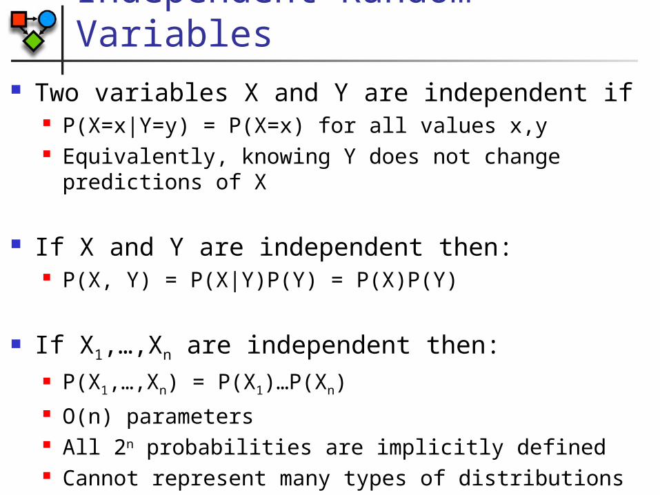
Independent Random Variables Two variables X and Y are independent if

P(X=x|Y=y) = P(X=x) for all values x,y Equivalently, knowing Y does not change predictions

of X

If X and Y are independent then: P(X, Y) = P(X|Y)P(Y) = P(X)P(Y)

If X1,…,Xn are independent then: P(X1,…,Xn) = P(X1)…P(Xn) O(n) parameters All 2n probabilities are implicitly defined Cannot represent many types of distributions

Conditional Independence X and Y are conditionally independent given Z

if P(X=x|Y=y, Z=z) = P(X=x|Z=z) for all values x, y, z Equivalently, if we know Z, then knowing Y does not

change predictions of X Notation: Ind(X;Y | Z) or (X Y | Z)

Conditional Parameterization S = Score on test, Val(S) = {s0,s1} I = Intelligence, Val(I) = {i0,i1}

I S P(I,S)

i0 s0 0.665

i0 s1 0.035

i1 s0 0.06

i1 s1 0.24

S

I s0 s1

i0 0.95

0.05

i1 0.2 0.8

I

i0 i1

0.7 0.3

P(S|I)P(I)P(I,S)

Joint parameterization Conditional parameterization

3 parameters 3 parameters

Alternative parameterization: P(S) and P(I|S)

Conditional Parameterization S = Score on test, Val(S) = {s0,s1} I = Intelligence, Val(I) = {i0,i1} G = Grade, Val(G) = {g0,g1,g2} Assume that G and S are independent given I

Joint parameterization 223=12-1=11 independent parameters

Conditional parameterization has P(I,S,G) = P(I)P(S|I)P(G|I,S) = P(I)P(S|I)P(G|I) P(I) – 1 independent parameter P(S|I) – 21 independent parameters P(G|I) - 22 independent parameters 7 independent parameters

Biased Coin Toss Example Coin can land in two positions: Head or Tail

Estimation task Given toss examples x[1],...x[m] estimate

P(H)= and P(T)=1-

Assumption: i.i.d samples Tosses are controlled by an (unknown) parameter Tosses are sampled from the same distribution Tosses are independent of each other

Biased Coin Toss Example Goal: find [0,1] that predicts the data well

“Predicts the data well” = likelihood of the data given

Example: probability of sequence H,T,T,H,H

m

i

m

iixPixxixPDPDL

11)|][()],1[],...,1[|][()|():(

23 )1()|()|()|()|()|():,,,,( HPHPTPTPHPHHTTHL

0 0.2 0.4 0.6 0.8 1

L(D

:)

Maximum Likelihood Estimator Parameter that maximizes L(D:)

In our example, =0.6 maximizes the sequence H,T,T,H,H

0 0.2 0.4 0.6 0.8 1

L(D

:)

Maximum Likelihood Estimator General case

Observations: MH heads and MT tails Find maximizing likelihood Equivalent to maximizing log-likelihood

Differentiating the log-likelihood and solving for we get that the maximum likelihood parameter is:

TH MMTH MML )1():,(

)1log(log):,( THTH MMMMl

TH

H

MM

M

Sufficient Statistics For computing the parameter of the coin toss

example, we only needed MH and MT since

MH and MT are sufficient statistics

TH MMDL )1():(

Sufficient Statistics A function s(D) is a sufficient statistics from

instances to a vector in k if for any two datasets D and D’ and any we have

):'():(])[(])[('][][

DLDLixsixsDixDix

Datasets

Statistics

Sufficient Statistics for Multinomial

A sufficient statistics for a dataset D over a variable Y with k values is the tuple of counts <M1,...Mk> such that Mi is the number of times that the Y=yi in D

Sufficient statistic Define s(x[i]) as a tuple of dimension k s(x[i])=(0,...0,1,0,...,0)

(1,...,i-1) (i+1,...,k)

k

i

Dsi

iDL1

)():(

Sufficient Statistic for Gaussian Gaussian distribution:

Rewrite as

sufficient statistics for Gaussian: s(x[i])=<1,x,x2>

2

2

12

2

1)(),(~)(

x

eXpNXP if

2

2

222

2

1exp

2

1)(

xxXp

Maximum Likelihood Estimation

MLE Principle: Choose that maximize L(D:)

Multinomial MLE:

Gaussian MLE: m

mxM

][1

m

i i

ii

M

M

1

m

mxM

2)][(1

MLE for Bayesian Networks Parameters

x0, x1

y0|x0, y1|x0, y0|x1, y1|x1

Data instance tuple: <x[m],y[m]> Likelihood

X

Y

Y

X y0 y1

x0 0.95

0.05

x1 0.2 0.8

X

x0 x1

0.7 0.3

):][|][():][(

):][|][():][(

):][],[():(

11

1

1

M

m

M

m

M

m

M

m

mxmyPmxP

mxmyPmxP

mymxPDL

Likelihood decomposes into two separate terms, one for each variable

MLE for Bayesian Networks Terms further decompose by CPDs:

By sufficient statistics

where M[x0,y0] is the number of data instances in which X takes the value x0 and Y takes the value y0

MLE

0 1

10

0 1

][: ][:||

][: ][:||

1

):][|][():][|][(

):][|][():][|][():][|][(

xmxm xmxmxYxY

xmxm xmxmXYXY

M

m

mxmyPmxmyP

mxmyPmxmyPmxmyP

1

11

1

01

11

][:

],[

|

],[

||):][|][(

xmxm

yxM

xY

yxM

xYxYmxmyP

][

],[

],[],[

],[1

01

1101

01

| 10

xM

yxM

yxMyxM

yxMxy

MLE for Bayesian Networks Likelihood for Bayesian network

if Xi|Pa(Xi) are disjoint then MLE can be

computed by maximizing each local likelihood separately

ii

i miii

m iiii

m

DL

mPamxP

mPamxP

mxPDL

):(

):][|][(

):][|][(

):][():(

MLE for Table CPD BayesNets Multinomial CPD

For each value xX we get an independent multinomial problem where the MLE is

)( )(

],[|

][|][| ):(

Xx

xx

XX

Val YValy

yMy

mmmyYY DL

][

],[| x

xx M

yM i

y i

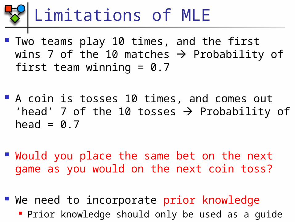
Limitations of MLE Two teams play 10 times, and the first wins 7

of the 10 matches Probability of first team winning = 0.7

A coin is tosses 10 times, and comes out ‘head’ 7 of the 10 tosses Probability of head = 0.7

Would you place the same bet on the next game as you would on the next coin toss?

We need to incorporate prior knowledge Prior knowledge should only be used as a guide

Bayesian Inference Assumptions

Given a fixed tosses are independent If is unknown tosses are not marginally

independent – each toss tells us something about The following network captures our

assumptions

X[1] X[M]X[2]…

0

1

][1

][)|][(

xmx

xmxmxP

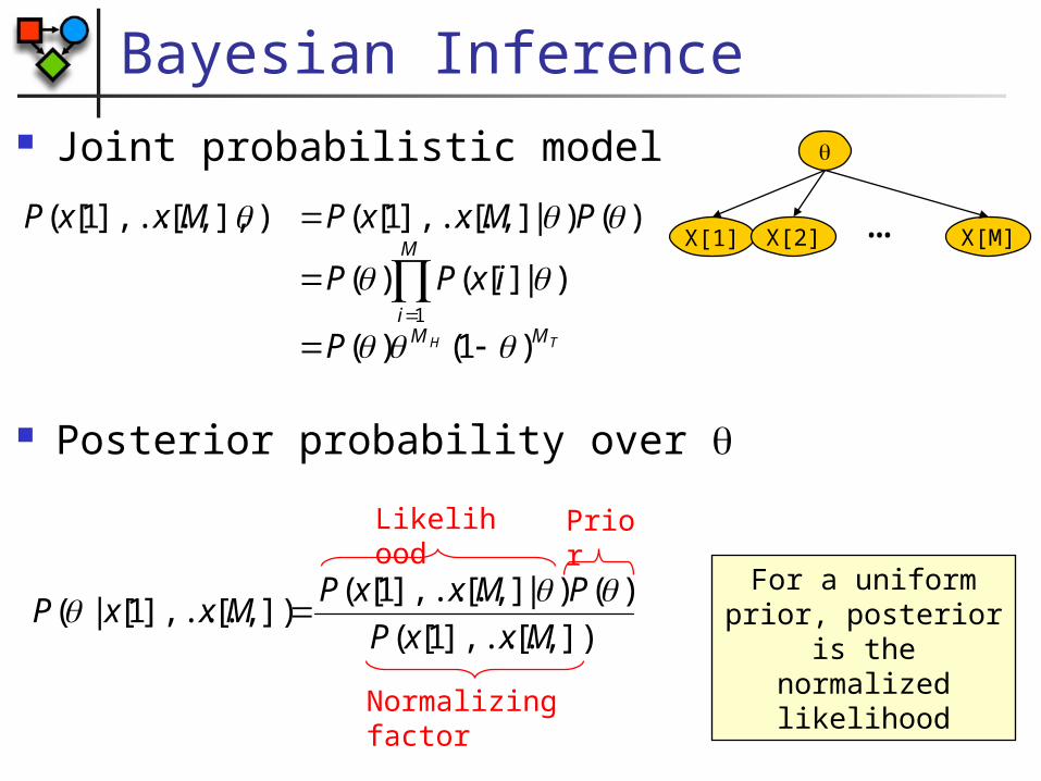
Bayesian Inference Joint probabilistic model

Posterior probability over

TH MM

M

i

P

ixPP

PMxxPMxxP

)1()(

)|][()(

)()|][],...,1[()],[],...,1[(

1

X[1] X[M]X[2] …

])[],...,1[(

)()|][],...,1[(])[],...,1[|(

MxxP

PMxxPMxxP

Likelihood

Prior

Normalizing factor

For a uniform prior, posterior is the

normalized likelihood

Bayesian Prediction Predict the data instance from the previous

ones

Solve for uniform prior P()=1 and binomial variable

dMxxPMxP

dMxxPMxxMxP

dMxxMxP

MxxMxP

])[],...,1[|()|]1[(

])[],...,1[|()],[],...,1[|]1[(

])[],...,1[|],1[(

])[],...,1[|]1[(

2

1

)1(])[],...,1[(

1)],[],...,1[|]1[( 1

TH

H

MM

MM

MMxxP

MxxxMxP TH

Example: Binomial Data Prior: uniform for in [0,1]

P() = 1 P( |D) is proportional to the likelihood L(D:)

MLE for P(X=H) is 4/5 = 0.8 Bayesian prediction is 5/7

)|][],1[(])[],1[|( MxxPMxxP

7142.07

5)|()|]1[( dDPDHMxP

0 0.2 0.4 0.6 0.8 1

(MH,MT ) = (4,1)

Dirichlet Priors A Dirichlet prior is specified by a set of (non-

negative) hyperparameters 1,...k so that

~ Dirichlet(1,...k) if

where and

Intuitively, hyperparameters correspond to the number of imaginary examples we saw before starting the experiment

k

kk

ZP 11

)( )(

)(

1

1

k

i i

k

i iZ

0

1)( dtetx tx

Dirichlet Priors – Example

0

0.5

1

1.5

2

2.5

3

3.5

4

4.5

5

0 0.2 0.4 0.6 0.8 1

Dirichlet(1,1)Dirichlet(2,2)

Dirichlet(0.5,0.5)Dirichlet(5,5)

Dirichlet Priors Dirichlet priors have the property that the

posterior is also Dirichlet Data counts are M1,...,Mk

Prior is Dir(1,...k) Posterior is Dir(1+M1,...k+Mk)

The hyperparameters 1,…,K can be thought of as “imaginary” counts from our prior experience

Equivalent sample size = 1+…+K The larger the equivalent sample size the more

confident we are in our prior

Effect of Priors

0.15

0.2

0.25

0.3

0.35

0.4

0.45

0.5

0.55

0 20 40 60 80 1000

0.1

0.2

0.3

0.4

0.5

0.6

0 20 40 60 80 100

Different strength H + T Fixed ratio H / T

Fixed strength H + T

Different ratio H / T

Prediction of P(X=H) after seeing data with MH=1/4MT as a function of the sample size

Effect of Priors (cont.)

0.1

0.2

0.3

0.4

0.5

0.6

0.7

5 10 15 20 25 30 35 40 45 50

P(X

= 1

|D)

N

MLEDirichlet(.5,.5)

Dirichlet(1,1)Dirichlet(5,5)

Dirichlet(10,10)

N

0

1Toss Result

In real data, Bayesian estimates are less sensitive to noise in the data

General Formulation Joint distribution over D,

Posterior distribution over parameters

P(D) is the marginal likelihood of the data

As we saw, likelihood can be described compactly using sufficient statistics

We want conditions in which posterior is also compact

)()|(),( PDPDP

)(

)()|()|(

DP

PDPDP

dPDPDP )()|()(

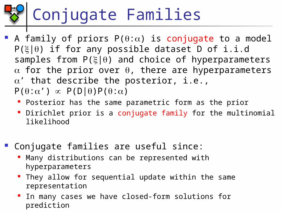
Conjugate Families A family of priors P(:) is conjugate to a model P(|) if

for any possible dataset D of i.i.d samples from P(|) and choice of hyperparameters for the prior over , there are hyperparameters ’ that describe the posterior, i.e.,P(:’) P(D|)P(:) Posterior has the same parametric form as the prior Dirichlet prior is a conjugate family for the multinomial

likelihood

Conjugate families are useful since: Many distributions can be represented with hyperparameters They allow for sequential update within the same

representation In many cases we have closed-form solutions for prediction

Parameter Estimation Summary

Estimation relies on sufficient statistics For multinomials these are of the form M[xi,pai] Parameter estimation

Bayesian methods also require choice of priors MLE and Bayesian are asymptotically

equivalent Both can be implemented in an online manner

by accumulating sufficient statistics

][

],[),|( ,

ipa

iipaxii paM

paxMDpaxP

i

ii

][

],[ˆ|

i

iipax paM

paxMii

MLE Bayesian (Dirichlet)

This Week’s Assignment Compute P(S)

Decompose as a Markov model of order k Collect sufficient statistics Use ratio to genome background

Evaluation & Deliverable Test set likelihood ratio to random locations &

sequences ROC analysis (ranking)

Hidden Markov Model Special case of Dynamic Bayesian network

Single (hidden) state variable Single (observed) observation variable Transition probability P(S’|S) assumed to be sparse

Usually encoded by a state transition graph

S S’

O’

G G0 Unrolled network

S0

O0

S0 S1

O1

S2

O2

S3

O3

Hidden Markov Model Special case of Dynamic Bayesian network

Single (hidden) state variable Single (observed) observation variable Transition probability P(S’|S) assumed to be sparse

Usually encoded by a state transition graph

S1

S2

S3

S4

s1 s2 s3 s4

s1 0.2 0.8 0 0

s2 0 0 1 0

s3 0.4 0 0 0.6

s4 0 0.5 0 0.5

P(S’|S)

State transition representation