learning bold response in fmri by reservoir computing paolo avesani 12, hananel hazan 3, ester...

LEARNING BOLD RESPONSE IN FMRI BY RESERVOIR COMPUTINGPaolo Avesani12, Hananel Hazan3, Ester Koilis3,

Larry Manevitz3, and Diego Sona12

1 NeuroInformatics Laboratory (NILab), Fondazione Bruno Kessler, Trento, Italy

2 Interdipartimental Mind/Brain Center (CIMeC), Università di Trento, Italy

3 Department of Computer Science, University of Haifa, Israel

2

fMRI – functional Magnetic Resonance Imaging

2011, November CS MSc University of Haifa

time

• Blood Oxygen Level-Dependent (BOLD) signal (oxygen hemodynamic response) is a measurement of the brain activity

• BOLD signal is recorded for each voxel inside the brain image

…

BOLD v1(t) Voxel 1

v2(t) Voxel 2

.

.

.

vN(t) Voxel N

fMRI Machine A sequence of stimuli Registered brain activity (over time)

3

Analysis of fMRI Data – Brain Mapping


• Highlighting areas of brain maximally relevant for a given cognitive or perceptual task

Relevant voxels are highlighted

Brain Map

BOLD

v1(t) Voxel 1

v2(t) Voxel 2

.

.

.

vN(t) Voxel N

4

GLM (General Linear Model) Method


• BOLD signal is reconstructed as a linear combination of input stimuli convolved with the expected ideal BOLD hemodynamic function (obtained theoretically).

GLM

Pre

dict

or Predicted BOLDsignal

Expected ideal BOLD

Stimuli sequence

Convolvedstimuli

sequence

)()(ˆ tXtv

)(1 tx

)(2 tx

5

Brain Mapping – GLM Method


• Good prediction accuracy indicates the relevance of the voxel for a given perceptual/cognitive task

Compare

Brain Map

Relevant voxels

Predicted BOLD

Original BOLD

)(ˆ tv

)(tv

GLM Approach Drawbacks• Prior assumption is made on the expected ideal BOLD

hemodynamic response• The ideal BOLD haemodynamics may vary for different

reasons• May lead to incorrect brain maps!!!

2011, November CS MSc University of Haifa 6

Expected Response

Real Responses

The Schema

• A predictor is trained to produce the BOLD voxel-wise given the sequence of stimuli based on a real training data

2011,November CS MSc University of Haifa 7

A A AB B B

time

train

Training data set

Pre

dict

or

]);;([ˆ 0 tStSftv

The Schema

• A predictor is trained to produce the BOLD voxel-wise given the sequence of stimuli based on a real data

• Good prediction accuracy indicates the relevance of the voxel for a given perceptual/cognitive task

2011,November CS MSc University of Haifa 8

B A BA B predict

Testing data set

Pre

dict

orCompare

Brain Map

Relevant voxels

Predicted BOLD

Original BOLD

)(ˆ tv

)(tv

?

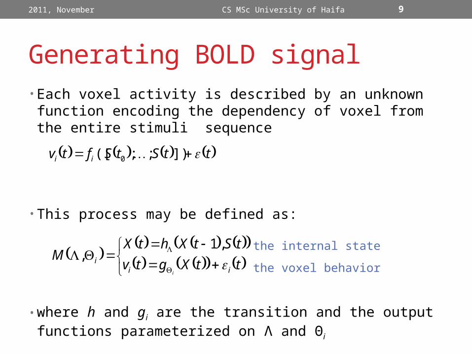
Generating BOLD signal• Each voxel activity is described by an unknown function

encoding the dependency of voxel from the entire stimuli sequence

• This process may be defined as:

• where h and gi are the transition and the output functions parameterized on Λ and Θi

ttStSftv ii ]);;([ 0


ttXgtv

tStXhtXM

iii

i,1

,the internal state

the voxel behavior

10

Reservoir Computing Model• Computational paradigm based on the recurrent networks of spiking neurons

• The recurrent nature of the connections project the time-varying stimuli into a reverberating pattern of activations, which is then read out by any learner (decoder) to generate the required BOLD signal

• Implementation details:• A Reservoir – an LSM network based on LIF neurons with fixed weights• Decoders – voxel-wise MLP trained with the resilient back-propagation algorithm


Reservoir

Voxel-wisedecoders

Input

hΛ

gΘi

X(t)S(t)

ttXgtv

tStXhtXM

iii

i,1

,

11

Experimental Material

• Synthetic datasets• Generated with a standard hemodynamic Balloon model plus

autoregressive white noise + some parameters adjustments• Both voxels related and not related to the stimuli were generated

• 3 different experiment designs:• Block, Event-Related, Fast Event-Related


sec0

a. Block design

sec0

b. Slow event related

sec0

c. Fast event related

12


• 5 different HRF shapes:• Baseline• Oscillatory• Stretched• Delayed• Twice


13


• Real datasets• Datasets collected on a real healthy subject performing a known

cognitive task (faces vs. scrambled faces).• A standard GLM approach was used to evaluate the relevance of

the selected voxels to a given task

• Evaluation• 4-fold cross-validation for each voxel• The prediction accuracy measured as a Pearson correlation

between the original and the reproduced BOLD signals averaged over all 4 folds

• RMSD values are calculated


Synthetic Datasets - Results

2011, June 1 CS MSc University of Haifa 14

Metrics

Voxels

Related

to

Stimuli

Noise Level ()

= 0.1 = 0.2 = 0.3 = 0.4 = 0.5

r (SD)

Yes0.707

(0.042)

0.533

(0.043)

0.468

(0.057)

0.350

(0.055)

0.292

(0.044)

No0.072

(0.046)

0.082

(0.051)

0.078

(0.038)

0.064

(0.048)

0.085

(0.058)

RMSD(SD)

Yes0.641

(0.091)

0.964

(0.073)

1.001

(0.064)

1.030

(0.063)

1.139

(0.037)

No1.413

(0.060)

1.374

(0.055)

1.389

(0.041)

1.438

(0.043)

1.388

(0.051)

• Event Related Design


2011, June 1 CS MSc University of Haifa 15

• Event Related Design



• Fast Event Related Design

• Block Design

Metrics

Voxels

Related

to

Stimuli

Noise Level ()

= 0.1 = 0.2 = 0.3 = 0.4 = 0.5

r (SD)

Yes0.423

(0.065)

0.288

(0.076)

0.277

(0.062)

0.208

(0.055)

0.170

(0.042)

No0.085

(0.032)

0.078

(0.018)

0.076

(0.026)

0.113

(0.041)

0.119

(0.049)

Metrics

Voxels

Related

to

Stimuli

Noise Level ()

= 0.1 = 0.2 = 0.3 = 0.4 = 0.5

r (SD)

Yes0.724

(0.043)

0.643

(0.046)

0.599

(0.065)

0.405

(0.054)

0.377

(0.050)

No0.045

(0.017)

0.090

(0.041)

0.062

(0.040)

0.066

(0.031)

0.057

(0.034)

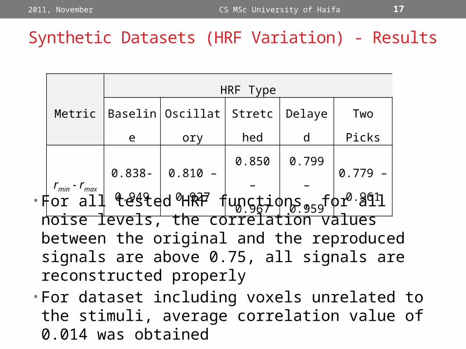
Synthetic Datasets (HRF Variation) - Results


MetricHRF Type

Baseline Oscillatory Stretched Delayed Two Picks

rmin - rmax

0.838-

0.949

0.810 –

0.927

0.850 –

0.967

0.799 –

0.959

0.779 –

0.961

• For all tested HRF functions, for all noise levels, the correlation values between the original and the reproduced signals are above 0.75, all signals are reconstructed properly

• For dataset including voxels unrelated to the stimuli, average correlation value of 0.014 was obtained

Real Datasets - Results


DesignVoxels Related to

Stimulir SD

BlockYes 0.568 0.062

No 0.094 0.044

Event Related Yes 0.348 0.053

No 0.056 0.042

Fast Event Related Yes 0.278 0.041

No 0.102 0.040

Real Datasets - Results


Relevant voxel

LSM

Real

Block

Irrelevant voxelBlock

PredictedReal

PredictedReal

Summary


Dataset Type Protocol

Accuracy by Voxel Type

Related to

Stimuli

Unrelated

to Stimuli

Both

Related &

Unrelated

to Stimuli

Synthetic Datasets

Block 100% 100% 100%

Slow ER 100% 100% 100%

Fast ER 100% 100% 100%

Oscillatory HRF 100% 100% 100%

Stretched HRF 100% 100% 100%

Delayed HRF 100% 100% 100%

Twice-Pick HRF 100% 100% 100%

Total Synthetic 100% 100% 100%

Real Datasets

Block 100% 92% 96%

Slow ER 96% 99% 98%

Fast ER 86% 88% 87%

Total Real 93% 94% 94%

All Total for All Sets 96.5% 97% 97%

• Percentage of correctly identified voxels based on calculated correlation values (r>0.15 – voxels related to the stimuli, otherwise – not related to the stimuli)

21

Next Steps

• Improve the analysis techniques for super fast event related design by introducing the reservoir computer training phase

• Include the entire brain into the analysis • Use reservoir computing for tracing signal history length


IDENTIFYING HUMAN MEMORY ENCODING MECHANISMS FROM PHYSIOLOGICAL FMRI DATA VIA MACHINE LEARNING TECHNIQUES

Asaf Gilboa12, Hananel Hazan3, Ester Koilis3,

Larry Manevitz3, and Tali Sharon2

1 Rotman Research Institute, Toronto, Canada

2 Department of Psychology, University of Haifa, Israel

3 Department of Computer Science, University of Haifa, Israel

23

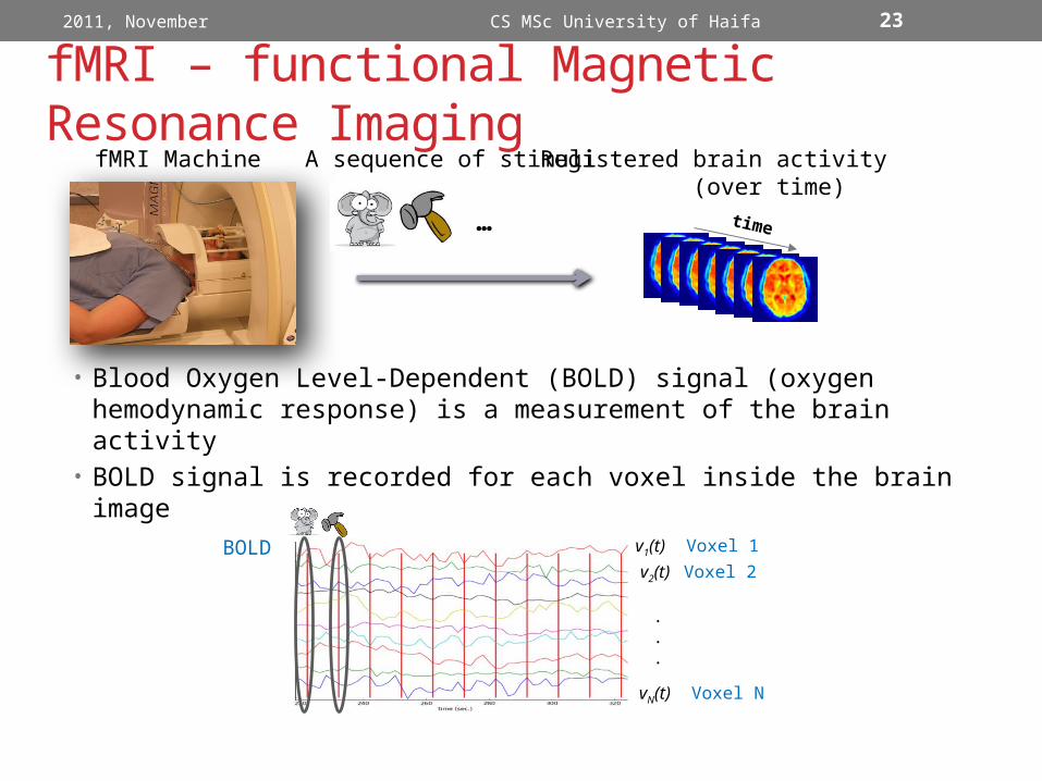
fMRI – functional Magnetic Resonance Imaging


time

• Blood Oxygen Level-Dependent (BOLD) signal (oxygen hemodynamic response) is a measurement of the brain activity

• BOLD signal is recorded for each voxel inside the brain image

…

BOLD v1(t) Voxel 1

v2(t) Voxel 2

.

.

.

vN(t) Voxel N

fMRI Machine A sequence of stimuli Registered brain activity (over time)

24

Analysis of fMRI Data• Brain decoding

• Prediction of the cognitive state given the brain activity

• Brain mapping• Highlighting areas of brain maximally related to some specific

cognitive or perceptual task

2011, November CS MSc, University of Haifa

time

predict

time

+generate

25

Areas of Research• Processing of senses: vision, hearing, perception• Physiology of cognitive functions: memory, decision

making, induction/deduction, categorization• Higher cognitive processes: executive attention, meta-

information processing


26

Memory Types


Procedural

Declarative

Memory

Unconscious procedures

Conscious recollection of facts and events

27

Declarative Memory Acquisition


EXPLICIT ENCODING

Neurocortex(Long-Term

Memory)

MTL (including hippocampus)

consolidation

It takes days to months to consolidate new information in the neurocortex

28

Declarative Memory Acquisition


FAST MAPPING Neurocortex

(Long-Term Memory)

Mom: Look at this yellow butterfly!

yellow

What about adults?

Tali Sharon, 2010 – adults with hippocampal lesions are able to learn new facts with Fast Mapping

29

Declarative Memory Acquisition (Sharon,2010) – Fast Mapping


30

Current Study


• Explore the neural correlates related to the FM (Fast Mapping) mechanism

• Compare the neurophysiological (fMRI) data collected from healthy adults performing FM (Fast Mapping) and EE (Explicit Encoding) tasks:• Is FM a complimentary mechanism for EE?• Does FM exist in healthy individuals?

31

Current Study – Materials (Sharon,2010)


• fMRI data of 24 healthy participants, 12 of them performing FM tasks, other performing EE tasks• FM task – “Is the inside of the lukuma red?”• EE task – “Remember the durion”

• Post-recollection success test is performed

32

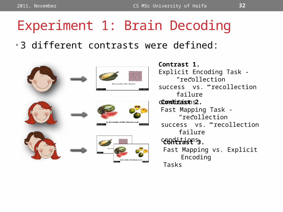
Experiment 1: Brain Decoding


• 3 different contrasts were defined:

Contrast 2. Fast Mapping Task - “recollectionsuccess” vs. “recollection failure”conditions.

Contrast 1. Explicit Encoding Task - “recollectionsuccess” vs. “recollection failure”conditions.

Contrast 3. Fast Mapping vs. Explicit EncodingTasks

33

• ML Classifier – stimulus prediction according to the brain image

• High classification accuracy is an indicator of information existence inside the data

Machine Learning - Classification


Classifier

Classifier

Classifier

Predicted Sample

Sample 1

Sample 2

Sample n

…

34

Classification Methods


• Multivariate classification, based on linear Support Vector Machine classifier:

• Classification accuracy as a measurement for the amount of relevant information

FMEE

Predicted class label

Classifier

n=517000

Given class label

35

• Dimensionality reduction –the most important features participate in the classification process

• 1000 top features were selected for all contrasts

Feature Selection


Feature Selector

36

• Three methods were explored:• Activity – the most active voxels are selected• Accuracy – voxels producing the most accurate predictions when

used for classification

• SVM-RFE (recursive-feature-elimination)

Feature Selection


FM EE

Predicted class label

Classifiervi

(1)

Prediction accuracy?

37

Final Architecture


• Multivariate classification, based on linear Support Vector Machine classifier, with feature selection:

FM EE

38

Classification Accuracy – Contrast 1 EE


Analysis Type

Feature

Selection

Method

Prediction

AccuracySD

Within-Subject

Accuracy 0.66 0.044

Activity 0.68 0.040

SVM-RFE 0.78 0.0237

Cross-Subject

Accuracy 0.61 0.0496

Activity 0.60 0.0452

SVM-RFE 0.73 0.0619

39

Classification Accuracy – Contrast 2 FM


Analysis TypeRanking

Metric

Prediction

AccuracySD

Within-Subject



SVM-RFE 0.81 0.0390

Cross-Subject



SVM-RFE 0.76 0.0307

40

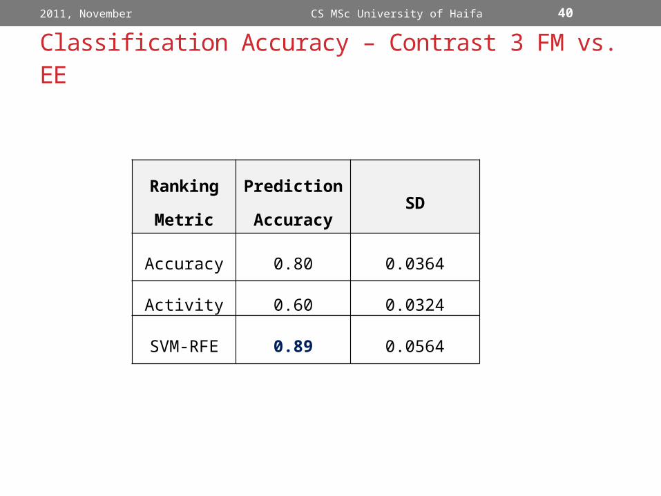
Classification Accuracy – Contrast 3 FM vs. EE


Ranking

Metric

Prediction

AccuracySD



SVM-RFE 0.89 0.0564

42

• Aim: to highlight the areas relevant for the required contrast, Contrast 1 FM or Contrast 2 EE

• Method: “searchlight” algorithm (Kriegeskorte, 2006)

Experiment 2: Brain Mapping


r=4

43

“Searchlight” Method


• Training classifiers on many small voxel sets which, put together, include the entire brain

• The search area includes voxel’s spherical neighborhood in radius r (r=4 in this study)

• SVM (Support Vector Machines) was used as the underlying classifier

• The accuracies of a classifier are used for highlighting the map voxels

44

Results – Contrast 1 EE


Hippocampus

45

Results – Contrast 2 FM


Temporal Pole

46

Experiment 3: Hippocampus vs. TP


• In this experiment, the classification was based on different brain areas

EE FM

Area

Prediction Accuracy

Within-

Subject

Cross-

Subject

All 0.778 0.732

Hippocampus Only 0.733 0.697

Temporal Pole Only 0.701 0.663

All w/o Hippo. 0.777 0.735

All w/o TP 0.777 0.734

Putamen Only 0.579 0.592

Area

Prediction Accuracy

Within-

Subject

Cross-

Subject

All 0.807 0.761

Hippocampus Only 0.723 0.686

Temporal Pole Only 0.756 0.713

All w/o Hippocampus 0.807 0.765

All w/o Temporal Pole 0.808 0.760

Putamen Only 0.567 0.557

47

Reverse pattern of FM and EE


• The same pattern of activity was detected in patients

Hippocampus Temporal Pole67

68

69

70

71

72

73

74

75

76

FM EE

Prediction success, %

Hippocampus Temporal Pole0

5

10

15

20

25

30

FM EE

Reduction in prediction success, %

48

Conclusions


• Using the multivariate methods for feature selection and classification purposes brought substantial increase to the classification performance

• Two different memory acquisition mechanism, FM and EE, are explored

• Fast Mapping network includes regions positioned more lateral in the temporal neocortex, and specifically in polar area, as opposed to medial temporal regions critical for episodic memory

learning bold response in fmri by reservoir computing paolo avesani 12, hananel hazan 3, ester...

Documents

bold original bold slide

bold voxelwise

brain image bold

brain activity bold

voxel activity

voxel behavior slide

highlighted brain map

ideal bold haemodynamics