ld du preez - repository.nwu.ac.za
TRANSCRIPT
1
Airborne radiometric surveys through the use of a handheld spectrometer fitted to a UAV
LD du Preez
orcid.org 0000-0001-9304-2805
Dissertation submitted in fulfilment of the requirements for the degree Master of Science in Environmental Sciences at
the North-West University
Supervisor: Dr SR Dennis
Graduation May 2018
23460318

2
Abstract Matter is made up of small particles called atoms of which some are unstable due to an
imbalance between protons and neutrons. This results in the particles being radioactive,
which will over time undergo radioactive decay in order to achieve a more stable state.
Measuring the radioactive decay of elements in the field is a physical and time-consuming
process that is conducted mainly through the use of handheld equipment such as
spectrometers and scintillometers. Alternative methods include aerial and car surveys, but
are more specialized, costly and situational.
This study is aimed at testing the viability of unmanned aerial vehicle (UAV) systems as an
alternative measuring platform. UAV systems are faster than walking, more accessible than
vehicles and cheaper than airplanes, making it theoretically a great platform for radiometric
surveys. Throughout the study, a total of three different UAV systems were used and
equipped with a handheld RS 230 spectrometer. A series of tests were conducted in order to
determine the measuring capabilities of the spectrometer at different heights above the
surface, as well the efficacy and accuracy of using a UAV system equipped with a
spectrometer.
A number of models were developed simulating the effect of a UAVs speed and height on
the spectrometers measuring accuracy. The effect of different radiological source sizes on
the measured radiation at a fixed height was measured. Furthermore, radiation was
measured at different heights using a constant radiation source. Results indicated that a
strong correlation existed between simulated and measured values.
The study provides sufficient evidence that the use of a UAV systems equipped with
handheld measuring equipment is capable of producing accurate and reliable radiological
data. However, the use of any elevated radiometric detection device has its limitations. An
area containing a homogenous radioactivity can be measured at greater altitudes than areas
having an inconsistent spread of radioactivity. For greater radiometric detection accuracy,
UAV systems used in areas with altering levels of radiation, are required to fly at lower
altitudes to be able to detect inconsistencies. The effect of the UAV system on the
spectrometer measuring capabilities has to be accounted for during data analysis.

3
Keywords
Airborne radiometric detection, UAV, New Machavie, RS 230.
Acknowledgements I would like to express my appreciation to:
Dr. R Dennis & Prof. I Dennis for their supervision and guidance.
Jaco Koch for all of his support and guidance
The team of Gyrolag (Gerhard & Laurent) for their support in the project designing
and field-testing.
New Machavie’s management for allowing the study to be conducted on their
property.
Haevic Drones for providing a UAV.
Pieter Holtzhausen for his assistance in the field.
Without their different inputs, this project would not have been successful.

4
Table of Contents
1 INTRODUCTION ......................................................................................................... 11
Research Problem ................................................................................................ 11
1.3 Aims and Objectives of this Study ......................................................................... 12
Layout of dissertation ............................................................................................ 13
2 Literature Review ......................................................................................................... 14
Basic radiometrics................................................................................................. 14
2.1.1 Alpha decay ................................................................................................... 17
2.1.2 Beta decay ..................................................................................................... 18
2.1.3 Gamma decay ............................................................................................... 21
Detection .............................................................................................................. 23
2.2.1 Radiometric detector ...................................................................................... 23
2.2.2 Environmental factors .................................................................................... 24
Radio Active material in gold tailings ..................................................................... 25
2.3.1 Uranium ......................................................................................................... 25
2.3.2 Thorium ......................................................................................................... 27
2.3.3 Potassium ...................................................................................................... 27
Previous work ....................................................................................................... 28
Data Representation ............................................................................................. 31
2.5.1 Scatter plots ................................................................................................... 32
2.5.2 Profile data representation ............................................................................. 32
2.5.3 Contour maps ................................................................................................ 32
2.5.4 Gridding ......................................................................................................... 33
Data sampling rates .............................................................................................. 33
Data Analysis ........................................................................................................ 34
2.7.1 Height correction ............................................................................................ 38
2.7.2 Circle of investigation ..................................................................................... 38

5
2.7.3 Edge detection ............................................................................................... 39
3 Study Area Description ................................................................................................ 40
Background information ........................................................................................ 40
3.1.1 Location and History ...................................................................................... 40
3.1.2 Climate .......................................................................................................... 41
3.1.3 Geology ......................................................................................................... 41
Site selection ........................................................................................................ 45
4 Materials and methods ................................................................................................. 46
Method of measurement ....................................................................................... 46
4.1.1 RS-230 Spectrometer .................................................................................... 46
4.1.2 Infotron IT 180 mini UAV ................................................................................ 46
Methods applied ................................................................................................... 47
4.2.1 Field of view estimation .................................................................................. 47
4.2.2 Effect of source size on measurements ......................................................... 49
4.2.3 Activity loss measurements with elevation. .................................................... 51
Measurement simulations ..................................................................................... 53
4.3.1 Elevation effect .............................................................................................. 54
4.3.2 Velocity effect ................................................................................................ 55
4.3.3 UAV measurement......................................................................................... 55
5 Results and discussion ................................................................................................ 57
Field of view .......................................................................................................... 57
5.1.1 Field of view results ....................................................................................... 57
Effect of source size on measurements ................................................................ 62
Activity loss measurements ................................................................................... 68
Measurement simulations ..................................................................................... 72
UAV measurements .............................................................................................. 75
Downscaling ......................................................................................................... 77
6 Conclusion and Recommendations .............................................................................. 79
7 References .................................................................................................................. 83

6
Abbreviations
𝑚. 𝑠−1 Meter per second
°C Degrees Celsius
AM Amplitude modulation
Ar Argon
BGO Bismuth Germinate oxide
Bq Becquerel
Bq/m² Becquerel per square meter
C Carbon
Ca Calcium
cm centimeter
cm³ Cubic centimeter
CPS Counts per second
Csl Caesium iodide
eV Electron volts
FM Frequency modulation
FOB Fraction of Background
FOV Field of View
FTA Fault Tree Analysis
g/T Gram per ton
GPS Global positioning system
GTK Geological Survey of Finland
He Helium
HGM Horizontal gradient magnitude
Hz Hertz
I Iodine
Ir Iridium
K Potassium
keV Kilo-electron Volt
kg Kilogram
km/h Kilometers per hour
m Meter

7
m³ Cubic meter
MeV Mega-electron volt
Mm Millimeter
NaI Sodium Iodide
Pa Protactinium
Pb Lead
PCA Principal Component Analysis
Po Polonium
PVC Polyvinyl chloride
RSD Radiation Survey Device
Sec Second
SNR Signal to noise ratio
Sv/h Sieverts per hour
Te Tellurium
Th Thorium
U Uranium
UAV Unmanned aerial vehicle
Α Alpha
Β Beta
Γ Gamma

8
List of Figures
Figure1: The structure of the atom (Lawson, 1999) ............................................................ 14
Figure 2: Carbon-14 decay sequence (Canadian Nuclear Safety Commission, 2012) ........ 16
Figure 3: Alpha decay (Based on Lawson, 1999) ................................................................ 18
Figure 4: Beta plus decay (Based on Lawson, 1999) .......................................................... 20
Figure 5: Beta minus decay (Based on Lawson, 1999) ....................................................... 21
Figure 6: Gamma decay (Based on Lawson, 1999) ............................................................ 23
Figure 7: Uranium decay series (after Koch, 2014) ............................................................. 26
Figure 8: Thorium decay series (after Koch, 2014) .............................................................. 27
Figure 9: Gamma analysis strategy (Erdi-Krausz & Nicolet , 2003) ..................................... 37
Figure 10: Circle of investigation at different altitudes. (Allyson, 1994) ................................ 39
Figure 11: New Machavie map location............................................................................... 40
Figure 12: Potchefstroom monthly rainfall ........................................................................... 41
Figure 13: New Machavie’s geology composition ................................................................ 43
Figure 14: Distribution of the Malmani Subgroup ................................................................. 44
Figure 15: Google earth view of New Machavie .................................................................. 45
Figure 16: Field of view ....................................................................................................... 48
Figure 17: Field of view experiment setup ........................................................................... 48
Figure 18: Spectrometer with smallest container ................................................................. 50
Figure 19: Container sizes .................................................................................................. 50
Figure 20: Spectrometer with largest container ................................................................... 50
Figure 21: Spectrometer with second largest container ....................................................... 50
Figure 22: Vertical activity loss test setup ............................................................................ 50
Figure 23: UAV over New Machavie ................................................................................... 52
Figure 24: Spectrometer connected to the Infotron 180 ....................................................... 52
Figure 25: Vertical activity loss test representation (UAV; New Machavie) .......................... 52
Figure 26: Pole activity loss measurements ....................................................................... 53
Figure 27: Line interval measurements ............................................................................... 53
Figure 28: Walking pole measurement setup ...................................................................... 54
Figure 29: Walking pole measurement setup ...................................................................... 54
Figure 30: UAV test flight at 5 meters .................................................................................. 56
Figure 31: Custom Octocopter ............................................................................................ 56

9
Figure 32: Field of view determination for a height of 1 meter ............................................. 58
Figure 33: Field of view determination for a height of 1.5 meter .......................................... 59
Figure 34: Field of view determination for a height of 2 meter ............................................. 60
Figure 35: FOV angle equation ........................................................................................... 61
Figure 36: Height response of circular sources ................................................................... 62
Figure 37: Line of best fit for the FOB values ...................................................................... 65
Figure 38: FOB equation representation for parameter a .................................................... 66
Figure 39: FOB equation representation for parameter b .................................................... 66
Figure 40: FOB equation representation for parameter c .................................................... 67
Figure 41: Fraction of background vs elevation of circular sources ..................................... 68
Figure 42: R value representation ....................................................................................... 69
Figure 43: UAV vs modelled activity loss ............................................................................. 70
Figure 44: Stationary pole vs modelled activity loss ............................................................ 71
Figure 45: Moving pole vs modelled activity loss ................................................................. 72
Figure 46: Simulated vs measured response at im elevation ............................................... 73
Figure 47: Simulated vs measured response at 3m elevation ............................................. 73
Figure 48: Simulated vs measured response at 5m elevation ............................................. 74
Figure 49: Effect of a UAV on a spectrometer ..................................................................... 75
Figure 50: UAV data vs simulated data ............................................................................... 76
Figure 51: Downscaling of 5 meter high measurements ...................................................... 77
Figure 52: New Machavie radioactivity distribution .............................................................. 78
Figure 53: Representation of the effect of FOV ................................................................... 78

10
List of Tables Table 1: Uranium decay series with half-lives and radiation type (after Grasty, 1979) ......... 26
Table 2: FOV observation radius ......................................................................................... 60
Table 3: FOV angle results.................................................................................................. 61
Table 4: Signal to noise ratio ............................................................................................... 64
Table 5: Equation parameter values .................................................................................... 65
Table 6: Representative parameter formula ........................................................................ 67

11
1 INTRODUCTION
The following chapter provides an introduction to the research problem, the aims and
objectives of the study and provides the layout for the dissertation.
Research Problem
Radiometric methods are based upon the measurement and detection of natural
radioactivity, with the focus upon gamma radiation, originating from three naturally occurring
radioactive elements: potassium, thorium and uranium. Radiation is formed during the
disintegration of unstable isotopes. During the disintegration three types of radiation are
emitted - alpha particles, beta particles and gamma rays. Alpha and beta particles can be
measured as the physical loss of particles within the element whereas gamma rays are
weightless, contain no charge and are classed as an electromagnetic radiation found at the
bottom of the electromagnetic spectrum with a frequency of 10²° Hz and a wavelength of
10ˉ¹² meters. The reason why gamma rays are preferred over alpha and beta particles is due
to the penetrating effect of gamma rays. Alpha particles have very little penetrating effect
and are absorbed within 10 cm of air. Beta particles have a higher penetrating effect than
alpha particles but will be absorbed in several meters of air. Gamma rays on the other hand
have a penetrating range of several hundred meters thus for field studies, providing a clear
idea of the isotopes producing the gamma radiation (Richards, 1981).
Obtaining radiometric data is a physical and time-consuming process that is conducted
mainly through the use of hand held equipment such as spectrometers and scintillometers.
Alternative methods such as aerial surveys are a viable option, but expensive with various
industrial sites having strict regulations concerning the use of aircraft at low altitudes. Aerial
surveying involves the measuring of gamma radiation emitted by the geochemical elements
in the upper 30 cm of the earth’s crust. Due to safety reasons the aircraft must be at a height
of 10m or more above the ground. As a result of the height difference the amount of gamma
radiation is greatly reduced. To compensate for the loss of radiation a spectrometer with a
higher sensitivity must be used. This requires a spectrometer containing a bigger crystal,
generally over 8.2 litres, which in turn increases the cost of the aerial survey (Richards,
1981).
Thus, the purpose of this dissertation is to develop a method of surveying that is cheaper
than aerial surveys and faster than physical handheld ground surveys. The proposed
method is to make use of drone technology and combine it with hand held equipment.

12
The testing will be conducted at the New Machavie Gold Mine tailing dams situated 22 km
outside the town of Potchefstroom. The mine was active from the 1930’s until the early
1940’s and was used to mine gold from the Black Reef Formation of the Transvaal
Supergroup. Uranium is a naturally occurring radioactive mineral that is commonly
associated with gold mining activities (Wendel, 1998). The chemical and physical processes
during gold mining result in the accumulation of radioactive minerals at certain stages during
the process, most commonly and in the case of the new Machavie Mine, at the tailing dam.
Although uranium is expected to be in large quantities, the occurrence of thorium and
potassium will also be measured in the tailing dam.
In 2013 an article was published describing an unmanned aerial vehicle (UAV) being fitted
with a radiation survey device (RSD). The purpose of the UAV was to serve as a
reconnaissance instrument in emergency situations. The new device was successfully
manufactured and tested. The RSD is capable of detecting dose rates between 10ˉ⁷ and 10ˉ¹
Sievert per hour and can detect surface contamination of 105 Bq/m² at a height of 100 m
(Bogatov, 2013). The study proved that an UAV can be fitted with radiation detectors and
accurately detect radiation. The success of a handheld spectrometer mounted onto a UAV
will need to be tested.
1.3 Aims and Objectives of this Study
The aim of this study is to determine whether mounting a handheld spectrometer onto a UAV
is a viable solution towards easier and faster radiation data collection. The specific
objectives for the study can be summarized as follows:
1. Determine handheld spectrometer detection capability at different heights vs.
different source sizes through stationary ground experiments.
2. Obtain accurate surface radiometric measurements along a predefined survey line,
which will be used as reference measurements.
3. The reference measurements will be compared to the experimental survey making
use of a handheld spectrometer and a drone. The experimental airborne survey will
be conducted at various heights to determine the resolution loss on the signal with
height.
4. Estimate the field of view (FOV) of the radiometric detector.
5. Process the experimental survey data and compare with the reference ground
survey.
6. Investigate the effect of the UAV flight speed on the recorded radiometric data.
7. Study the effect of noise generated by the UAV on the recorded data.

13
Layout of dissertation
This dissertation will contain the following chapters:
1. Introduction
2. Literature
Research about different radiometric methods, previous scientific studies, nature of
radiation, radioactive elements and detection methods.
3. Study Area
Description of the study area and test sites in terms of previous work conducted as
well as geology, climate and topography.
4. Materials and Methods
Description of project procedure and the equipment necessary for the project.
5. Results and Discussion
Discussion of the results obtained and the applicability in geophysical surveys
6. Conclusions and Recommendations
Discuss the conclusion that is derived from the results as well as the method
analysis. Based on the conclusion and shortcomings a recommendation will be
provided as to how the project can be improved.
7. References
8. Appendices

14
2 Literature Review
Basic radiometrics
Everything that is observed in the visible universe is comprised of endless numbers of
atoms. These atoms are combined into specific arrangements to form molecules and then
matter (Borgese, 1977:236). Some of these arranged elements give rise to matter that has
the unique characteristic of being radioactive. Radioactivity is a phenomenon that occurs
when radioactive minerals (manmade and natural) undergo the process of decay (Murray &
Holbert, 2015:31–46).
Atoms consist of three components as seen in Figure1: protons, neutrons and electrons.
Protons and neutrons are found in the centre of the atoms and together form the nucleus.
Electrons are much smaller and lighter than protons and neutrons and are located in orbits
around the nucleus (Borgese, 1977:236). The number of protons that an element contains is
known as the atomic number and is used to define the element, but it is possible for an
element to vary in mass through the addition or removal of neutrons. The number of protons
and neutrons is known as the mass number and represents the sum total of nucleons in the
nucleus of the atom. Although the atomic number of an element is required to remain at a
constant number to maintain the identity of the element the number of neutrons can differ
without compromising the identity of the element. This variation in atomic mass while having
a continuous atomic number is known as isotopes (Lawson, 1999:1–20).
Figure1: The structure of the atom (Lawson, 1999)

15
Some variations of elemental isotopes are unstable due to an imbalance between protons
and neutrons and will undergo radioactive decay to achieve a more stable state over time;
these isotopes are known as radio-isotopes. During the decaying proses, the radioactive
isotopes will become weaker as the decay process continues; once the element has reached
a stable state it will cease to produce radiation resulting in the radioactive activity to be zero.
The activity of a radioactive element refers to the number of disintegrations within the
radioactive material per unit time. The elements activity is measured in Becquerels (Bq),
where 1 Bq = 1 disintegration per second.
The law of radiometric decay is an equation that is used to express the decrease of atoms
situated within a radioactive element:
𝑁𝑡 = 𝑁0𝑒−𝜆𝑡
𝑁𝑡 Number of atoms remaining after a specified time (t)
𝑁0 Number of atom at time t=0
𝜆 The decay constant of radioactive elements
Another related constant is the half-life (𝑇21) of an element and is represented by the
following equation (Erdi-Krausz & Nicolet, 2003):
𝑇21 =
0.693
𝜆
Every radioactive element decays at a different rate and will determine the time it will take to
reach a stable state. The time it takes for an element to lose half of its activity from the start
of decaying is known as the radiological half-life. Some the elements only reach radiological
half-life after billions of years and some only after a fraction of a second. Examples of
elements with radical different decaying periods are iodine-131 and plutonium-239. Iodine-
131 will reach its half-life in only eight days whereas plutonium-239 will only reach its half-life
after 24 000 years.

16
Radioactive elements decay at an exponential rate and will experience several half-lives
before reaching a stable state and becoming non-radioactive. Figure 2 depicts the
exponential decay curve of carbon-14, with each half-life at 5700 year intervals (Canadian
Nuclear Safety Commission, 2012).
Figure 2: Carbon-14 decay sequence (Canadian Nuclear Safety Commission, 2012)
Small elements are commonly more stable when containing the same number of protons
and neutrons, but a larger element in a stable state contains a higher number of neutrons
than protons (Canadian Nuclear Safety Commission, 2012). The vast majority of isotopes
found on earth are in a stable state. The reason being that most of the short-lived isotopes
have already decayed throughout the history of the earth. There are currently 320 different
isotopes where 270 isotopes are in a stable state and 50 occurring naturally as
radioisotopes.
Radioactive decay can be divided into two different forms: particle or electromagnetic
radiation. Both are emitted from the nuclei of atoms into the surrounding environment. The
emitted radiation can either have an ionizing or non-ionizing effect:
Ionizing radiation is the process whereby the interaction of radiation with atoms can
upset the charge and electron/proton balance of atoms. This occurs when radiation

17
knocks electrons out of their orbits around the atom leaving the atom in a more
positive state. These electrically charged atoms and molecules are known as ions.
Ionizing radiation is considered to be hazardous to humans and can be caused by
natural as well as manmade radioactive minerals.
Non-ionizing radiation contains lower amounts of energy than that of ionizing
radiation and is not capable of producing ions. Examples of non-ionizing radiation
include radio waves, infrared, sunlight and visible light. Television stations, global
positioning systems, AM and FM radio, baby monitors and the earth’s magnetic field
are other forms of non-ionizing radiation and are not considered to be hazardous to
human health.
There are several different types of ionizing radiation, but the three most common forms are
gamma (), alpha (α) and beta (β) radiation. Although these different types of radiation differ
greatly from each other (as discussed further on) they are measured using the same units
known as electron volts (eV). Electron volts refers to the energy that an electron obtained
within a vacuum after it has been accelerated by a voltage of one volt. This unit of energy is
a tiny amount and is equivalent to 1.6 x 10⁻¹⁹ joules, but a more practical unit that is used for
radiometrics is mega-electron volt (MeV) and is equivalent to 106 eV. Even this unit is a tiny
amount of energy and it would take 2.5 x 10¹³ MeV to raise the temperature of one gram of
water by 1°C (Murray & Holbert, 2015:31–46).
2.1.1 Alpha decay
During the process of alpha decay, the nucleus of the atom emits a particle known as an
alpha particle. The particle is comprised of two protons and two neutrons, identical to that of
a helium atom (Richards, 1981). Alpha decay occurs mostly in atoms that contain a heavy
nucleus with a large proton to neutron ratio. The reason being that the nuclear forces holding
the nucleus together are very short ranged. Thus when too many nuclides are residing within
the nucleus, the nuclear forces will be weak between the individual nuclides and will not be
able to hold them together (Lawson, 1999.1–20).
The alpha particle is a very stable configuration of particles, leaving the parent atom in a
more stable state as well as reducing the proton to neutron ratio (Murray & Holbert,
2015:31–46). The alpha particle does not serve as an external threat to humans due to its
limited penetrating effect and will be absorbed within 10 cm of air or the outer layer of human
skin (Richards, 1981). However, when a source of alpha radiation is present within a human
body the energy will fully be absorbed into the bodily tissue (Canadian Nuclear Safety
Commission, 2012).

18
As seen in Figure 3 when uranium 234 decays two protons and neutrons are produced and
form a subsystem within the uranium’s nucleus. The binding forces of the two protons and
neutrons are stronger than any of the remaining binding forces within the nucleus and the
alpha particle is seen as a separate particle trapped within the nucleus. The separate
particle or alpha particle will tunnel through the nucleus away from the nuclear forces and
will be ejected from the nucleus by Coulomb forces. The combined 230 remaining protons
and neutrons within the nucleus will be identified as Thorium 230 (Hübsch, 1997).
Figure 3: Alpha decay (Based on Lawson, 1999)
2.1.2 Beta decay
Beta particles contain a negative charge and are identical to electrons differing only in origin.
Beta particles originate from the nucleus whereas electrons are found in orbit around the
nucleus. A Beta particle contains a higher penetration effect than an alpha particle, reaching
a few meters before being absorbed and is capable of penetrating the skin, transferring the
energy into the skin cells (Richards, 1981). Beta decay occurs when there are too many
neutrons or protons within the nucleus of the atom. The decay process will transform the
neutrons or protons into each other, with the aim of placing the atom in a more stable state.
It is believed that an isolated proton is stable and will not decay over time. When a neutron is
isolated, it is in an unstable state and will decay over a short time, reaching its halftime within
Alpha particle
He 4
2
230
98 Th
Daughter nucleus
Parent nucleus
U 234
90 Decay
Proton
Neutron

19
10.5 minutes (Murray & Holbert, 2015:31–46). To achieve stability within the atom, one of
two beta decay processes will occur, known as beta minus and beta plus.
Beta plus
Beta plus decay is the transformation of a proton into a neutron by emitting a positron (see
Figure 4). Unlike alpha decay, beta decay requires the emission of multiple particles to
balance the radioactive process. These particles include a daughter element as well as a
positron and a neutrino. The result of the positron emission is the decrease in atomic
number by one due to the proton turning into a neutron, whilst the atomic mass remains
constant.
A positron is the antiparticle of an electron and after being emitted will only travel a short
distance before being annihilated through contact with an electron. The positron, as well as
the electron, will both disappear, but the combined energy of both particles (equivalent to
511 keV) will be dispersed in the form of gamma rays.
The neutrino was first proposed in 1930 but was only verified in 1956. The purpose of the
neutrino was to explain certain observations that were made within radioactive decay and to
balance the energy levels (Lawson, 1999:1–20), but taking the laws of conservation into
account a number of constraints had to be fulfilled for the particle to exist: The particle had to
be neutral for the reaction was already balanced. The energy values of the electrons were at
the allowed maximum; therefore, the mass of the particle had to be extremely small. The
neutrino had to be an antiparticle to compensate the creation of the electron particle, and
finally, the neutrino had to be a subatomic particle with a half-integral spin to couple the total
final angular momentum to the initial spin (Loveland et al., 2006). With all these constraints it
has made the neutrino particle extremely hard to detect (Lawson, 1999:1–20).
N 𝑝 + 𝒆+ + v
N Original atom
𝑝 Daughter atom
𝒆+ Positron
v Neutrino

20
Beta minus
Beta minus decay is the conversion of a neutron into a proton by emitting an electron/beta
particle from within the nucleus due to a surplus of neutrons. Similar to that of beta plus
decay multiple particles are emitted during the radioactive process, but instead of a positron,
an electron is emitted together with a neutrino. The emission of an electron or beta particle
balances the charge of the nucleus and the neutrino balances the energy levels (see Figure
5). The result of the process increases the atomic number by one while the atomic mass
stays the same. The beta minus process can be written as follows (Lawson, 1999:1–20):
N 𝑝 + 𝒆− + 𝑣
N Original atom
𝑝 Daughter atom
𝒆+ Positron
𝑣 Antineutrino
Decay 124
53 I
Parent nucleus
Neutron
Proton
Excited
Daughter nucleus
𝒆+
124
52 Te*
Positron/ Beta particle
v
Neutrino
Figure 4: Beta plus decay (Based on Lawson, 1999)

21
2.1.3 Gamma decay
Gamma radiation differs significantly from that of Alpha and Beta radiation. Alpha and Beta
radiation consists of particles whereas gamma rays are a form of electromagnetic radiation
containing no charge or mass and can penetrate several hundred meters of air (Richards,
1981). Light and radio waves are also found within the electromagnetic spectrum, the
difference being the energy levels as well as the wavelengths (Lawson, 2013:19–34).
Gamma rays are found at the bottom of the spectrum with an average frequency of 10²² Hz
and a wavelength of 10⁻¹⁴ meters making them shortest wavelengths of the spectrum while
containing the highest amounts of energy (Richards, 1981).
Gamma rays originate from the rearrangement of protons and neutrons in atomic energy
levels. As previously discussed atoms naturally move towards a stable state where protons
and neutrons are in the proximity in equal numbers. If there is a more than optimal number
of neutrons in the nucleus, then it would be favourable for the neutrons to convert into
protons by beta minus decay. When the neutron is converted into a proton, the nucleus will
be in an energized state that is reduced to a stable state by the emitting of a gamma ray
Decay 234
90 Th
Parent nucleus
Neutron
Proton
Excited
Daughter nucleus
Electron/ Beta particle
234
91 Pa*
𝒗
𝒆−
Antineutrino
Figure 5: Beta minus decay (Based on Lawson, 1999)

22
(see Figure 6). In contrast, when there is a surplus of protons in the nucleus, the protons will
convert into neutrons through beta plus decay lowering the energy level of the nucleus and
also emitting a gamma ray (Lawson, 2013:19–34).
The Interaction of gamma rays with matter also differs from that of the Alpha and Beta
particle interactions. Alpha and Beta particles will undergo many individual interactions with
matter whereas gamma rays will move through matter with only one or two interactions, if
any at all. If gamma rays interact with matter it happens according to three processes:
photoelectric absorption, Compton scattering and pair production (Lawson, 1999:1–20).
Compton scattering refers to the decrease of gamma ray energy levels due to interaction
with electrons situated in the outer layer of atoms, absorbing a part of the gamma ray energy
levels. The reduced gamma ray continues with the decreased energy levels and is still able
to interact with other atoms (Richards, 1981). The amount of energy absorbed during the
Compton scattering interaction varies between interactions and directly affects the exiting
angle of the gamma ray. The smaller the energy reduction is, the smaller the exiting angle
will be and vice versa.
Photoelectric absorption occurs when gamma rays are completely absorbed by the atom’s
outer layer electrons. The complete absorption usually occurs after the energy levels have
decreased due to Compton scattering (Richards, 1981).
Pair production refers to the total absorption of gamma rays with energy levels surpassing 1
MeV. During pair production, both a positron and an electron will be produced at the same
time, but the positron will be destroyed after a while leaving the atomic electron to produce
two gamma rays of 511 KeV. The secondary electrons will then go on to produce ionization
of the material (Lawson, 1999:1–20).

23
Figure 6: Gamma decay (Based on Lawson, 1999)
Pa*
Excited daughter nucleus
Detection
2.2.1 Radiometric detector
Gamma-ray photons are neutral and do not create a direct ionization or excitation of the
materials through which they pass. Thus for the detection of gamma rays, it is critical that the
gamma-ray photons interact with the electron absorbing material within the detectors,
allowing the material to entirely or partially absorb the energy of the gamma ray (Knoll &
Wiley, 2000).
Normally a Sodium Iodide (NaI) crystal is used as the electron absorbing material within the
detector; the crystal has a high density that increases the interactions of gamma rays
(Richards, 1981). Alternatively, Bismuth Germinate oxide (BGO) crystals have been used as
an electron absorbing material in medium-energy detection device applications. A gamma
spectrometer is required to have a) a significant detection efficiency b) a good energy
resolution c) a low sensitivity to the room background. The BGO crystal delivers good results
on all of these requirements. Compared to the NaI the BGO crystal contains a higher density
and atomic number, making the BGO crystal more efficient in interacting with gamma rays.
Although the BGO crystal is more efficient, it also has its flaws. The crystal has a lower light
Neutron
Proton
Excited
Daughter nucleus
234
91 Pa*
Daughter nucleus
234
91 Pa
y
Emitted y photon

24
output due to the crystals high refraction index as well as the emission spectrum that is
shifted towards longer wavelengths. Large BGO crystals also have a chance to contain air
bubbles causing the light to be unevenly distributed throughout the crystal (Corvisiero et al.,
1990:478–484). It is essential for the electron absorbing materials within gamma detection
devices to contain a luminescent capability; whenever these crystals are introduced to a
gamma ray it will interact with the crystal and produce a flash of light found in the ultraviolet
range of the spectrum. The intensity of the light is measured by a photomultiplier and is
converted into an electrical signal. The electrical impulse produced by the detector is
proportional in amplitude to the intensity of the flash and thus proportional to the energy of
the original gamma ray.
A height pulse analyzer measures the amplitude of each pulse. The measured amplitude of
the pulse is then used to determine the counter or channel that will be used by the
spectrometer to register the pulse. The number of channels that a spectrometer may have,
varies between two and several hundred, but most handheld spectrometers contain only
three channels: Thorium, Uranium and Potassium, coupled with a total count channel
(Richards, 1981).
2.2.2 Environmental factors
Any material that is situated in between a radioactive source and a detector could cause
alterations to the measured radiation. During aerial surveys, the increase of height has a
major effect on the attenuation of gamma rays due to the interactions with suspended
elements, and this needs to be accounted for.
Overburden also has an effect on the attenuation of gamma rays; dense vegetation can
reduce gamma rays by 35% whilst snow cover of 10 cm will have the same effect as 10
meters of air.
The change of temperature will also affect gamma rays. Lower temperatures increase the
density of air, causing higher numbers of interactions, while higher temperatures will
decrease air density, causing fewer interactions.
Soil moisture can cause major alterations in gamma ray surveying. When soil moisture
increases by 10% the number of gamma rays leaving the soil will decrease by 10%.
Alternatively, radon particles attach themselves to dust particles that are suspended in the
air. During precipitation the dust particles are brought down to the ground possibly causing
uranium measurements to be increased by more than 2000%. Therefore, it is recommended
that surveys should be conducted at least 3 hours after it has rained so that the abnormal
surface activity can decay (Erdi-Krausz & Nicolet, 2003).

25
Radio Active material in gold tailings
New Machavie forms part of the Witwatersrand basin where gold mining is linked with the
occurrence of radioactive elements (Wendel, 1998:87–92). The mine produced five gold
bearing tailing dams, each containing fluctuating levels of radioactive material. The most
important natural occurring radioactive minerals that are brought to the surface during gold
mining operations are the elements originating from the uranium and thorium decay series
as well as potassium (Kamunda et al., 2016:138). Uranium, Potassium and Thorium are also
the only natural occurring radioisotopes that produce gamma rays that contain sufficient
energy and have a high enough intensity to be measured by airborne surveys (Minty,
1997:39–50). Potassium is deemed as a crucial radioactive mineral contributing significantly
to human exposure but does not fall under any decay series (Kamunda et al., 2016:138).
2.3.1 Uranium
Uranium is found throughout the earth’s crust with an abundance of 2.7 g/T. Due to the
radioactivity of uranium, the element is commonly found in association with its decay
products. The occurrence of uranium in gold-bearing ores would have been the result of at
least three geological processes: Firstly the uranium minerals would have been concentrated
into almost pure blocks of uranium, the uranium blocks would then have been weathered
into a granular detrital form and finally due to gravity the weathered uranium minerals would
have been deposited into reefs in the Witwatersrand basin as weathering products. The
presence of water during the forming of the reefs played an essential role throughout the
geological processes: Water has a significant effect on the chemical transformations of
minerals as well as a physical effect. Water contributes to the weathering of rocks as well as
the transportation of the weathered materials (Wendel, 1998:87–92).
The discovery of uranium in the Witwatersrand dates back to 1915, but the mineral was not
considered very hazardous even with the knowledge of it being a radioactive mineral
(Wendel, 1998:87–92). South Africa started extracting uranium from gold mines in 1951, but
it never became a primary source of export due to the low price of uranium. The high costs
of establishing and running uranium mines, competing markets and the ready availability of
uranium due to the dismantling of nuclear weapons after the cold war, limited the demand of
uranium (Dasnois, 2012:32).
The uranium decay series begins with Uranium 238 in an unstable state and ends with Lead
206 in a stable state. Figure 7 indicates the possible decay routes that can be followed by
the decay of uranium to reach a stable state. Although there are many possible routes to
achieve a stable state, only one will most likely be followed and is seen as the main route.

26
Figure 7: Uranium decay series (after Koch, 2014)
The route consists of 14 steps and is indicated in Table 1 along with the type of radioactive
decay and the half-life duration. From these 14 steps, six of them decay through beta minus
decay while the remaining eight decay by emitting an alpha particle (Arazo et al., 2016). The
uranium decay series also occurs over a wide span of time periods stretching from 𝑈92238
decaying over 4.5 billion years to reach 𝑇ℎ90234 , while 𝑃𝑜84
214 will decay in a time span of 164
micro seconds to form 𝑃𝑏82210 (Murray & Holbert, 2015:31–46)
Table 1: Uranium decay series with half-lives and radiation type (after Grasty, 1979)
Isotope Radiation Half life
𝑈238 𝑇ℎ234 𝑃𝑎234 𝑈234 𝑇ℎ230 𝑅𝑎226 𝑅𝑛222 𝑃𝑜218 𝑃𝑏214 𝐵𝑖214 𝑃𝑜214 𝑃𝑏210 𝐵𝑖210 𝑃𝑜210 𝑃𝑏206
α β β α α α α α β β α β β α Stable
4.507 x 10⁹ y 24.1 d 1.18 m 2.48 x 10⁵ y 7.52 x 10⁴ y 1600y 3.825 d 3.05 m 26.8 m 19.7 m 1.58 x 10ˉ⁴ s 22.3 y 5.02 d 138.4 d
Isotopes constituting less than 0.2 per cent of the decay products are omitted

27
2.3.2 Thorium
Thorium is a heavy metal found widely throughout the earth and is viewed as one of the
most vital resources for nuclear energy programs. Thorium is usually found in the minerals:
Monazite, Xenotime and Bastanasite. These minerals commonly make up a sizable fraction
of other elements such as aluminium, iron, lanthanides and actinides (Alipour et al.,
2016:19–29). Thorium is three times more abundant than uranium and is estimated by the
World Nuclear Association Website (accessed: 15 Sep 2016) to have a global joint mass of
6,355,000 tons with South Africa contributing 148,000 tons. Thorium is mildly radioactive and
found in Group 3 of the periodic table containing an atomic mass of 232.0381 with an atomic
number of 90 (Poole, 2004). The decay sequence as seen in figure 8 begins at Thorium²³²
and ends at Lead²º⁸.
Figure 8: Thorium decay series (after Koch, 2014)
2.3.3 Potassium
There are 24 known isotopes of potassium however only three occur naturally: 𝐾39, 𝐾40,
𝐾41. From the known isotopes only one is radioactive (𝐾40). The 𝐾40 isotope can decay
through two distinct processes each reaching a different end result/element. The first decay
process undergoes electron capture coupled with positron emission to produce stable 𝐴𝑟40.
The second decay process is through beta emission reaching the stable state of 𝐶𝑎40. In
practice radioactive potassium is used to determine the age of geological structures as well
as serving as a radioactive indicator in studies of weathering. Within a human body of 70 kg

28
an estimated 4400 nuclei of 𝐾40 decay per second making 𝐾40 the largest source of natural
radioactivity within the human body, topping that of 𝐶14 (Melorose et al., 2015)
Previous work
The combination of radiometric detection devices with UAVs (unmanned aerial vehicles) is
not a new concept and has been the centre of research in the past. However, most of these
studies were conducted with the aim to produce a product that can be used during a time of
crisis where the movement of humans is limited or restricted and not necessarily with the
purpose of developing a fast, accurate, efficient and cost-effective method of detecting
radioactivity with a commercial end goal.
In 2008, the STUK-Radiation and Nuclear Safety Authority of Finland published a study
where they mounted a commercial Csl radiation surveillance system onto a small-unmanned
aerial vehicle. The UAV system was a Patria mini-UAV, capable of cruising at speeds of 60
km/hˉ¹ at altitudes varying between 50 and 120 meters. Only one person is required to
operate the easy to use UAV system from a ground control station. The UAV system
constantly provided the operator with data originating from the radiation detector and
provided the operator with sufficient information to supervise and assess the mission status.
The detector that was used for the study was a commercial handheld radiation detector
containing a CsI probe that was set to measure the total count in cps every sec. Ground
measurements were taken to be compared to the UAV measurements as a function of
source-to-detector distance. The test was conducted at an airfield in Finland and aimed to
measure radioactive fallout in the air. The test started at an altitude of 150 meters and
decreased as the test progressed. The UAV flew over a Cs point source on the ground,
which was represented by peaks in the data whenever the UAV flew over the source. The
data had a strong correlation with altitude and increased accordingly with the decrease in
altitude. The test concluded that the detector was capable of detecting Cs and Ir point
sources on the ground, but admitted that a manned aircraft is more capable of mapping
radiation fallout. The study proved to be a success when aimed towards identifying radiation
hot spots for the health and safety of workers and the public (Pöllänen et al., 2009:340–344).
The Nuclear Safety Institute of Russia combined a md4-1000 UAV with a spectrometer and
two Geiger Muller counters with the goal to produce a radiation survey device that could be
used by rescue forces for reconnaissance in cases of an emergency. When choosing an
operating platform, the UAV had to fulfil certain criteria. Firstly, the UAV had to be easy to
control so that a non-professional pilot could operate the UAV; the UAV had to be reliable;
29
and finally, it had to be within a reasonable price range. The radiation survey device (RSD)
that was used during the project was developed by the Scientific and Industrial Centrum and
had to be able to operate within areas with large gamma dose intervals (10ˉ⁷ - 10ˉ¹ Sv/h). To
reach the requirement both a Geiger Muller counter and a spectrometer had to be flown
simultaneously. The spectrometer measures dose rates that range between 10ˉ⁷ and 10ˉ⁴
Sv/h, whereas the Geiger Muller counters measure dose rates between 10ˉ⁴ and 10ˉ¹ Sv/h.
The data analysis for the RSD was developed so that during the flight the UAV would send
location points with the corresponding dose rates to the operator for immediate
interpretation, but with a data packet loss of 5%. More accurate data analysis is conducted
once the UAV has landed and all the radiometric data can be extracted from the RSD. The
test proved to be a success and could detect a Cs point source with an activity of 10⁹ Bq
under 50 meters and a Cs surface contamination with an activity of 10⁵ Bq/m² according to
selected criterion below the height of 100 m (Bogatov and Mazny, 2013:4–6).
The Unmanned Systems Lab at Virginia Tech America developed a radiation remote
sensing system in response to the Fukushima disaster. The purpose of this system was to
limit the dangers for the first responders as well as to provide data to plan the actions of the
response team efficiently. For the carrier UAV, they used an Aeroscout B1-100 helicopter
coupled with a Sodium-iodide scintillating type detector. The detector measured the radiation
count every second for the duration of the mission. The study focused on two different
approaches in identifying radiation sources. The first approach focused on the localization of
a point source whereas the second approach focused on generating a complete radiation
map of an area. The system proved to be successful in the preliminary test, but
unfortunately, no complete tests were conducted with unshielded radioactive sources
(Towler et al., 2012:1995–2015).
The Geological Survey of Finland (GTK) commissioned an airborne radiometric study.
RadiaOy, a company that specializes in geophysical surveys and remote sensing with UAVs,
performed the study in the summer and autumn of 2016. The objective of the study was to
test the applicability of a radiometric system coupled with a UAV. The test area was at a
mine due to the elevated levels of uranium within the mines tailing dams. The radiometric
detection system that was used for the study was a D230A spectrometer, a product of
Georadis. The UAV was a custom-built quad-copter capable of carrying the 3.5 kg
spectrometer for 40 min, and could move at a speed of 10 m.sˉ¹.
Prior to the test, a measurement integration time of five seconds was chosen for the
sampling time. It was based on the UAVs movement speed during the flight (3-5 m.s). The
movement speed had to exceed that of a walking person (1.4-2 m.s) to make it a more

30
efficient technique. Initially, the spectrometer was placed 20 cm above the ground for 60
seconds to produce a base reading which was then compared to the measurements from
the spectrometer attached to the UAV at an altitude of 5 meters.
Initial comparison of the data indicated that the intensity of the measurements taken 20 cm
above the source was ten times greater than the intensity measured at an elevation of five
meters. The data measured at an elevated altitude was normalized and resulted in a higher
intensity than the ground measurements. The examiners described the intensity as a result
of overlapping material. The field of view of the elevated spectrometer included an area that
contained the peak radiometric anomaly of the tailings, increasing its intensity.
Data analysis was done through the use of GammaPros software and started by
• Combining all detectors values to produce the total yield.
• Merging four adjacent channels to produce 256 channel data.
• Normalizing the total count utilizing the time of measurements.
• Calculation of X and Y coordinates
• Compute and correct coordinates due to spectrometer movement.
• Determination of flight time and profile distance
• Store data in a format that is suitable for mapping as well as the combined 256 channel
spectra.
The data produced various total intensity images where some exhibited similarities between
them reflecting the geological background of the area, while others were not as clear. The
total intensity of gamma radiation indicated similarities, whereas uranium indicated some
similarities. Intensity maps of thorium and potassium were not as clear, questioning the
reliability of the measurements.
The objective of the study was to determine whether the use of a UAV system is a viable
substitute for walking and meant that many of the correction methods that are normally used
should be absent. The increase of height as well as variations were not taken into account
and could be the biggest defect of the survey. The height determination of the UAV wasn’t
accurate due to the laser altimeter influencing the UAVs stability and the use of outdated
digital terrain models during the flight. Despite the restrictions, the study concluded that a
UAV coupled with a radiometric detection device could serve as a feasible method for the
mapping of total radiometric intensity (Pirttijärvi & Oy, 2016)

31
All of the previous studies concluded that the use of a UAV as a detection platform is a
plausible alternative towards measuring radioactivity. However, differing from this study,
most of the previous studies were conducted with the aim to identify hotspot areas for times
of crisis and not for commercial use where accuracy is essential. The intensity of the
radiation may also differ from those of the previous studies. Because most of the previous
studies were primarily motivated to be used during times of crisis the amount of occurring
radiation will vary from the radiation that is to be found in nature or in tailing dams. The study
done by the Geological Survey of Finland proved that a UAV can be used over tailing dams,
but at a limited altitude. Unfortunately, the study did not account for accuracy and solely
focused on the possible usage of UAV technology for radiometric surveys. The current study
will focus on not only the usability of UAV systems, but also the accuracy of the measured
data.
Data Representation
Gamma-ray spectrometry data can be represented in a variety of ways that allows
interpretation of grids and radioelement profiles. Before the digital era (the 1980s) gamma
data was presented using contour maps and profiles. These methods still offer advantages
that makes them a viable representation method in today’s world. However, the progress of
digital technology provided a new platform to present data that benefits from digital image
processing techniques. Some of these techniques can be thought of as routine methods to
be used for most gamma representation. However, there is no universal technique that can
be applied to all gamma-ray mapping applications. Experimentation with different techniques
is vital to establish a method that is most suitable for specific requirements.
Before gamma-ray data can be represented, it has to be converted to a coordinate system,
map datum or map projection. By converting the data, we can accurately plot the data
according to its location on the earth. The conversion of data became important after the
integration of Global Positioning Systems (GPS) into geophysical surveys. Before GPS
systems were introduced the positioning of surveys was estimated by referencing aerial
photographs. The accuracy of these surveys was poor when compared to surveys done in
modern times. A GPS uses a variety of geocentric datum systems (Such as World Geodetic
System 1984) to estimate its position. Geocentric systems function on the concept that the
centre of the earth represents the true centre of gravity and plots position accordingly.
Representing radiometric data is commonly done through the use of one or multiple
methods. These methods include scatter plots, profiles, contour maps and grids (Erdi-Krausz
& Nicolet, 2003).

32
2.5.1 Scatter plots
Scatterplot graphs are the most useful way to display a relationship between two quantitative
variables. The values that represent one variable appear on the horizontal axis. The values
that represent the other variable are placed on the vertical axis (Moore et al., 2009). When
working with radiometric data, scatterplot graphs are a useful method to analyze the inter-
relationships between radioelements and to identify clusters and trends in the data.
However, the increase of radioelement concentration will result in greater scatter on the
graphs. This is because the error in the raw counts of radiometric data is Poisson distributed,
such that their amplitude increases with the square root of the detected count rate (Erdi-
Krausz & Nicolet, 2003).
2.5.2 Profile data representation
Profile data representation is commonly used for airborne spectrometric surveys. The use of
a profile representation is beneficial because it enables the interpreter to display the data at
full spatial resolution. Arithmetic combinations of radioelement channels and one-
dimensional filters can be used to enhance anomalies or reduce noise within the profile.
Profile plots can be stacked to provide the interpreter with visualizations that allow the
interpretation of inter-relationships between radioelements. The lithology of the study area is
commonly presented with stack profiles enabling easy analysis and correlation between the
anomalies and the lithology.
Multiple profile lines can be positioned next to each other to produce a single map. Each of
the profile lines represents a flight line that is referenced by (x,y) coordinates. However, the
height of the measuring equipment must be taken into account to prohibit the overlapping of
individual profile lines. The use of multi-profile line maps is extremely beneficial when
anomalies need to be identified (Erdi-Krausz & Nicolet, 2003).
2.5.3 Contour maps
In the past when an airborne survey was conducted the data was drawn by hand in the form
of contours. The quality of the drawing was directly influenced by the skill and experience of
the draftsman and could only be done by specialists. During the 1960s computer-based
contour maps replaced the hand-drawn maps and although image presentations of airborne
geophysical data is far more popular in modern times, the use of contour maps has not
completely been replaced. Contour mapping requires little space for storage and is
sometimes preferred when amplitude values need to extracted from data. The use of contour
maps is also advantageous when an undistorted presentation of an anomaly shape is
required.

33
Contour maps are produced by dividing the measured area into a grid. All the values within
every grid block are interpolated at a predetermined contour interval. Once the interpolation
is complete, the contour lines are drawn by connecting interpolation points that share similar
values. To prevent the contour lines from being ragged, the grid sizes need to be small in
comparison with the overall map size. The smaller the individual grids, the smoother the
lines will appear to be and vice versa (Erdi-Krausz & Nicolet, 2003).
2.5.4 Gridding
Gridding is the interpolation of data based on a mesh covering a surveyed area, each grid
node within the mesh contains a value. The data points that are captured within each grid
node determine the value of the node. The number of data points obtained within a node is
not necessarily the same number as the node next to it. Once the value of a node has been
established a contour can be generated between two nodes situated next to each other.
Alternatively, a rendered picture can represent each node without generating a contour.
Gridding can be represented by a variety of algorithms, but not every algorithm is suited to
represent airborne surveys. A suitable algorithm should be able to maintain the values that
have been assigned to the nodes while providing a smooth transition between them. An
example of an appropriate algorithm for gamma-ray spectrometric data is Kriging:
Radioactive decay has a random probability distribution that can be statistically analyzed but
cannot be precisely predicted. Kriging is an interpolation technique that assumes that the
direction and distance between the radiometric data points reflects a correlation that explains
a variation in the surface. The Kriging algorithm fits a mathematical function to data points
within a specific radius to determine an output value for each location. Kriging is commonly
used in soil sciences as well as geology but should be suitable for gamma-ray spectrometric
data (Erdi-Krausz & Nicolet, 2003).
Data sampling rates
During any elevated radiometric survey, the speed and altitude of the aircraft/UAV, as well
as the sampling time of the detector, are important influencing factors when accurate data is
a necessity. It is suggested that after the spatial wavelength or exploration sample size has
been established, the altitude of the aircraft/UAV is optimized at twice the spatial
wavelength. Based on this it is then possible to select from several combinations of sampling
times and speeds represented by:

34
∆𝑡 = ℎ/4𝑉
∆𝑡 Sample time in seconds
h Selected altitude in meters
V Aircraft’s or UAV’s speed in meters per second
After the combination has been determined and the UAV has been selected, the size of the
detector must be selected to produce viable counting statistics.
When the size of an anomaly is required, the anomaly can be thought of as a wavelength.
Therefore, the equation for determining the minimum wavelength of an anomaly is
represented by:
𝜆𝑚 = 2𝑉∆𝑡
𝜆𝑚 Anomaly size or minimum wavelength
∆t Sample time in seconds
V Aircraft’s or UAV’s speed in meters per second
When measuring count rates an acceptable standard deviation is said to be 10%−+ (Killeen,
1979:163–230)
Data Analysis
There is no single universal strategy that correctly interprets gamma radiological data, but it
is a process that has been influenced by various contributing factors throughout a survey.
The quality of data, survey area, and the purpose and scope of the interpretation significantly
affect the analysis of gamma rays.
Geographic Information Systems are now able to support the analysis and interpretation of
gamma radiation using image processing techniques. The enhancement techniques of these
systems are intended to assist visual interpretation and are a useful method to support
radiometric data analysis. Some of these techniques include mean differencing, principle
component analysis and regression that allow the interpreter to enhance small variations
that would have gone otherwise unnoticed. Other capabilities such as pattern recognition

35
use edge detection, classification and cluster analysis to automatically identify anomalies
and radioelement units.
Annotation of unit boundaries
After the gridded radiometric data has been enhanced, a GIS system can be equipped to
display the raster images and manually interpret the boundaries of distinct units and display
them as vector polygons.
Mean Differencing
Analyzing the radiometric elements (K, Th and U) within each interpreted unit will allow
information to be extracted from the data that is not immediately visible. The simplest of
analysis methods is to investigate the deviations from the unit means. Thorium, Uranium and
Potassium’s mean concentrations are determined for each unit and are subtracted, leaving
the residuals that are then imaged. If a large deviation occurs, it could be an indication of
geological processes (weathering, otherwise magma diversity) or it could be an error that
occurred during the mapping of unit boundaries.
Regression analysis
The effects of geological processes within the units can be removed by subtracting
regression models that were developed by forming single or multiple linear regression
models based on the estimated radioelement concentrations.
Classification techniques are based on pre-defined meaningful classes that have been
identified with respect to ground observations. The deciding rules for the distribution of these
classes are based on sample sites that are considered to be representative of the classes.
The use of classification techniques has been widely applied for the analysis of multispectral
image data originating from satellites orbiting the earth.
Figure 9 represents one of the many possible variations to accurately interpret gamma
spectrometric data. Based on Figure 9 the first step to interpreting gamma data is to
emphasize the overall change that occurs within the radioelement concentrations. Pseudo-
color coding, ternary mapping, contrast stretching and gradient enhancement are all
techniques that will contribute to the completion of the objective. Whenever gamma radiation
is masked by environmental factors such as water or overlaying material, the use of
arithmetic combinations, such as sum-normalized and ratios, can be used between different
data points to remove inconsistencies in the radiation response.

36
Multiple enhancements should preferably be used to determine all relevant features since no
single enhancement can adequately describe all relevant features (Erdi-Krausz & Nicolet,
2003).
The second step in the data interpretation is to outline all radiological anomalies as well as
areas that share similar data values. To substantiate the outlining of the radiological data
requires the use of the total count grid gradient that may be associated with the boundaries
of geological structures or soil units.
The application of principle component analyses, regression, or mean-differencing on each
of the outlined units will identify anomalies and enhance the gamma-ray responses against
the background variations. Based on the analysis of the data, the annotations of the unit
boundaries can be more accurately refined. Alternatively, by using pattern recognition
techniques, such as supervised classification and clustering, anomalies and units can be
identified.
The final step requires the integration of geological data into the gamma interpretation as
well as all other relevant information. To produce a visual interpretation, Geographic
Information System software can be used to display the radiometric data, topography,
geology, unit boundaries and anomalies as layers over each other.
When viewing the display results, special attention must be given to the topography and the
geomorphology of the area. The relation of these two layers governs the control and the
distribution of radiological elements. Data measured from material that has been transported
through human activities must be separated from data measured from bedrock formations.

37
Figure 9: Gamma analysis strategy (Erdi-Krausz & Nicolet , 2003)
In addition, when interpreting radiological data the interpreter must be aware of the
environmental factors that may influence the data accuracy; these include soil moisture
content, vegetation, alluvium and different weather exposures that can affect the data from a
homogeneous geological unit.
Whenever an important element shows an anomaly, which has a questionable source, the
anomaly must be checked by employing ground truthing. Ground truthing entails that the
source position of the anomaly must be checked by a radiometric detector on the ground.
The importance of ground truthing is enhanced by accurately displaying small areas of

38
radiation inconsistencies whereas areal measurements may indicate the same area as a
homogenous radiation zone. When areal measurement indicates an anomaly, ground
truthing can be conducted by employing a handheld spectrometer (Erdi-Krausz & Nicolet,
2003).
2.7.1 Height correction
During airborne surveys, the height of the detector changes constantly, possibly influencing
the gamma data. To compensate for the change in height the data needs to be corrected to
an insignificant height difference. Different heights that are typically reached during survey
flight can differ exponentially from each other. The following equation is used to determine
count rates at a nominal survey height:
𝑛 = 𝑛0𝑒−𝜇(𝐻−ℎ)
𝜇 Attenuation coefficient (per meter)
𝑛0 Observed count rate at STP height (h)
𝑛 Corrected count rate for the nominal survey terrain clearance (H)
This equation is suitable to be used in testing areas with an infinite source, areas with
homogenous topography and an altitude range between 50 and 250 meters (Erdi-Krausz &
Nicolet, 2003).
2.7.2 Circle of investigation
To accurately determine the counting rates of a test area the number of particles that cross a
certain point per unit time, also known as the fluence rate, has to be converted to a count
rate. The conversion requires knowledge about the detection cross-section of the detector at
a specified energy as well as the detector’s angular response. These requirements are
especially important when working with detectors that measure according to asymmetrical
geometries, such as the one used during this study.
The detection cross-section, also known as the circle of investigation, refers to the volume of
material that is measured directly underneath the detector during an aerial survey. As the
altitude of the detector increases the size of the circle of investigation increases accordingly
(as seen in Figure 10) but at the cost of signal intensity. During the measurement of a

39
homogenous infinite source, the increase of elevation will reach a point where no further
practical increase in intensity will occur.
The topography of the surrounding area can have a major influence resulting in inaccurate
measurements. To quantify the variations in topography Allyson, 1994 developed a
numerical formulation to compensate for the change in topography based on the most
commonly found geometries. However, this study was conducted on a mostly homogenous
source and requires no alterations according to topography changes (Allyson, 1994:1–293).
Figure 10: Circle of investigation at different altitudes. (Allyson, 1994)
2.7.3 Edge detection
Horizontal gradient magnitude (HGM), also known as an edge-detection filter, is an analysis
method used to help interpret gridded data sets as well as line-based profiles. The use of
this method allows the interpreter to identify anomalies in data that contains steep declines.
The analysis is commonly used in identifying gravitational anomalies, but can also be used
to analyse radiometric data. Horizontal gradient magnitude is represented by the following
equation (Beamish, 2016:75–86):
𝐻𝐺𝑀 = √(𝑑𝑥)2 + (𝑑𝑦)2
HGM Horizontal gradient magnitude
dx x-derivative
dy y-derivative

40
3 Study Area Description
Background information
3.1.1 Location and History
The New Machavie mine is a gold mine situated near the town of Potchefstroom in the North
West Province (Figure 11). The mine was active for 40 years extracting gold from the Black
Reef formation until the 1940s. During the excavations, the mine unearthed a total of 5147
kg of gold (Bever, 1997) and produced five tailing dams with a combined mass of about 2.5
million tons of processed materials (Aucamp, 2003:1–60).
Over the 40 years active period the New Machavie mine was operated by several
companies reaching a combined mining depth of 150m. The Black Reef quartzites were
mined in stretches from the northeast towards the southwest, dipping at an angle of 8-10˚ in
the southeast direction. Basal conglomerates up to 6.5 meters thick were mined by making
use of three trending channels spanning from the northeast towards the southwest (Bever,
1997).
Figure 11: New Machavie map location

41
3.1.2 Climate
South Africa is known as a semi-arid to arid country receiving an average rainfall of 500 mm
per annum, well below the world average of 860 mm. Furthermore, the rainfall is unevenly
distributed throughout the country with 65% of the country receiving less than 500 mm and
20% receiving less than 200 mm of rain (Annandale & Nealer, 2011). Potchefstroom
receives the most rain during the summer periods. The Geography Department at the North-
West University measured the last 30 years of monthly rainfall which is represented in Figure
12. On average, the Potchefstroom area receives an annual precipitation of 564 mm.
Figure 12: Potchefstroom monthly rainfall
Potchefstroom has a yearly average temperature of 16.9 °C, with the hottest temperatures
occurring during January, averaging 22.2°C. The coldest temperatures of the year occur
during June, with an average of 9.6°C.
3.1.3 Geology
The New Machavie mine is situated in an area underlined by of a variety of carbonic and
sedimentary rocks (see Figure 13) including limestone, dolomite, shale, quartzites. All of
these rock types form part of the Ghaap-Taupone-Chuniespoort Group also known as the
Malmani-Campbellrand carbonates (Figure 14), which is a subgroup of the Transvaal
Supergroup (Eriksson & Altermann, 1998:179–188). The Transvaal Supergroup contains a
0
20
40
60
80
100
120
Rai
n (
mm
)
Month
Monthly rainfall

42
mixed siliciclastic-carbonate ramp formed during a period when the area was covered by a
shallow-water shoreline or lagoon resulting in a low gradient slope (Wright & Burchette,
1998:1–5). The ramp grades upwards into a vast carbonate platform that is being overlaid by
a banded iron-formation. The supergroup was deposited onto the Kaapvaal craton consisting
of gneiss, granitoids and greenstone belts (Summer & Beukes, 2006:11–22). It is believed
that the Transvaal Supergroup is one of earth’s first major carbonic platforms (Schröder et
al., 2006:23–54).
The Malmani Subgroup is divided into five formations (Oaktree, Monte Christo, Frisco,
Eccles and Lyttelton) and is differentiated based on the chert content, stromatolite
morphology and the shale and chert-breccia horizons (Dirks & Berger, 2013:109–131).
These formations contain a variety of sequences, each representing periods where the
Kaapvaal Craton was submerged by water. There is a total of 12 sequences, each varying in
thickness with most sequences containing a variety of widespread carbonic rocks (Summer
& Beukes, 2006:11–22).
The New Machavie area contains only two of the five formations, with the Oaktree Formation
being the oldest followed by the Monte Christo Formation ( Anhaeusser et al, 2006). The
Oaktree formation has been estimated to have been deposited about 2588 million years ago.
The lower part of the Oaktree Formation forms part of the first geological sequence together
with lowermost Reivilo Formation, and the upper Blackreef Formation (Summer & Beukes,
2006:11–22). The thickness of the Oaktree formation varies between 100 and 150 meters
and is deposited on top of the Black Reef Formation. The Black Reef Formation is
comprised of quartzites and conglomerates and is a point of interest for mining companies
due to its gold-bearing ores. The Oaktree Formation consists of chert-poor dolomitic rocks
interbedded with shale layers thinner than 2 meters. The shale layers are carbonaceous and
contain two tuff layers thinner than 30 cm near the stratigraphic top (Dirks & Berger,
2013:109–131).
The second geological Formation that divides the New Machavie area is the Monte Christo (
Anhaeusser et al, 2006). The Monte Cristo Formation is a stromatolitic dolomite Formation,
rich in chert and contains oolite beds near its base. The Monte Cristo Formation like the
Oaktree Formation is interbedded with a thin shale layer thinner than 50 cm. The Formation
also contains a 5-meter thick layer of sheared-breccia in a dolomitic matrix (Dirks & Berger,
2013:109–131). The upper part of the Oaktree Formation together with the entire Monte
Cristo Formation and the middle Reivilo Formation make up the two to five geological
sequences (Craton et al., 2006:11–22).

43
Figure 13: New Machavie’s geology composition

44
Figure 14: Distribution of the Malmani Subgroup

45
Site selection
New Machavie was identified as an appropriate study area due to previous studies
conducted by North West University allowing for easy access. The New Machavie area
contains several tailing dams and selecting an appropriate tailing dam is based upon the
radioactive count emitted by the tailings, as well as the accessibility and condition of the
tailing dam's surface. Tailing dam T1 was initially selected to be used during the study but
was rejected due to the surface being inconsistent, containing individual tailing heaps on top
of the surface of the tailing dam, potentially producing inconsistent data. The tailing dam also
produced less radioactivity than the newly selected tailing dam. The new tailing dam T2 is
situated 280 meters South-West of T1 as seen in Figure 15. Although the tailing dam is
smaller in the overall surface area than T1 dam, it has a similar width of about 500 meters.
Figure 15: Google earth view of New Machavie
T1
T2

46
4 Materials and methods
Method of measurement
4.1.1 RS-230 Spectrometer
The detection device that was used during this study was an RS-230 handheld
spectrometer, a product of Radiation Solutions Inc. The RS-230 contains 103 cm³ bismuth
crystal rather than a Sodium-Iodine crystal. In comparison to Sodium-Iodine, a Bismuth
crystal has a higher density allowing more interactions with electrons, as well as gamma
rays resulting in a higher absorption percentage. The 103 cm³ bismuth crystal delivers 80%
of the performance of a 390-cm³ Sodium Iodide crystal. Bismuth crystals are more
commonly used within larger portable detection devices and are three times more powerful
than a Sodium Iodide crystal of the same size (Knoll & Wiley, 2000:816). The RS-230 has
two detection modes: survey and assay. The survey mode measures the sum total of all
disintegrations that occur in the surrounding area and is represented as the total count at a
rate of one measurement per sec. The assay mode measures the amount of potassium (K),
Uranium (U) and Thorium (Th) that is present in the area. Uranium and Thorium are
measured in parts per million whereas Potassium is measured as a percentage. The
detector also contains a 1024 radiometric channel coupled with a strong processor.
4.1.2 Infotron IT 180 mini UAV
The IT180-120 Unmanned Aerial Vehicle (UAV) that was used during the experiment is a
product of Infotron. The gasoline-driven IT180 was designed to be operated in extreme
weather conditions including heat, 60 km/h wind gusts, rain, snow and can be operated
during the day or night. The UAV has a flight time of 120 min and can carry a payload of up
to 5 kg. The working temperature of the UAV ranges from -10°C up to 40°C and the UAV
can reach a maximum speed of 70 km/h. The UAV is currently used by many industries
around the world, as well as firefighters in France.

47
Methods applied
4.2.1 Field of view estimation
As previously mentioned, the field of view (FOV) or circle of investigation is the area that is
observed by the radiometric detector during a survey. Knowing the field of view is crucial for
establishing the flight lines and determining the fluence rates. This will ensure that the
smallest number of lines will be flown to optimize the survey time and save money. The key
to elevated radiometric measurements is to find a balance between accuracy and efficiency.
If the surveyed area is too large, meaning that the UAV is too high, the data quality will be
dramatically reduced, possibly missing anomalies. However, if altitude and quality are
balanced the measurements will be fast and efficient, at a minimal cost to accuracy.
To calculate the RS 230 spectrometer’s FOV, an experimental test was developed to find the
maximum reach for the spectrometer’s detection radius.
The experiment started by identifying an area that contains a low homogenous radiometric
count rate as a testing platform. The spectrometer was connected to a pole marked with
three height intervals (1, 1.5 and 2 meters).
Initially, a control was established by measuring the radiometric decay of the area with no
radioactive source present. The control consisted of three measurements, one at each
height interval and the spectrometer was left for three minutes per height.
Once the control was established, a radioactive source was introduced and placed 12
meters away from the pole. After 2 minutes, the radioactive source was moved one-meter
closer to the pole. After 24 minutes, the radioactive source was directly underneath the
spectrometer as seen in Figure 17. After the 2-minute measuring period, the spectrometer
was moved again, but this time in the opposite direction, increasing the distance away from
the spectrometer after every 2 minutes. The spectrometer remained fixed at a predetermined
height and wasn’t moved until all required measurements were taken for the specific height.
Twenty-five measurements were taken in total per height interval, with 12 measurements
measured on each side of the spectrometer and one measurement taken directly
underneath the spectrometer. Figure 16 illustrates the experiment using sketches.

48
Figure 17: Field of view experiment setup
Once the data had been collected and plotted, data analysis techniques were applied to
determine the angle at which the spectrometer observes the surrounding area. The
Horizontal gradient magnitude analysis technique was used and is represented by:
𝐻𝐺𝑀 = √(𝑑𝑥)2 + (𝑑𝑦)2
HGM Horizontal gradient magnitude
dx x-derivative
dy y-derivative
1 m
Side view
2 m
Legend
Radiation Source
1 m interval pins
2 m high pole
RS 230 Spectrometer
Top view
1 m
Figure 16: Field of view

49
The horizontal gradient magnitude provides values representing the gradient of the plotted
values. The representative values were used to identify a distance point on the x axis where
the values dropped dramatically indicating the edge of the spectrometers detection range.
4.2.2 Effect of source size on measurements
As previously discussed, an increase of altitude increases the field of view as well as
decreasing the accuracy of the measurements. Due to the decrease in accuracy, some
anomalies that are situated within the field of view will be blended in or overshadowed by the
background noise.
Thus, a test was conducted to determine the loss of accuracy with the increased of field of
view. The purpose was to identify the height at which the background data would
overshadow a predetermined amount of radioactive source.
The test was conducted by measuring the amount of radiation emitted from a fixed source at
different height intervals. The test was repeated four times, with varying amounts of
radioactive material. The setup of the test consisted of a 2-meter pole with 20 cm height
intervals. The purpose of the pole was to keep the spectrometer centred above the
radioactive source and to serve as a height indicator. The spectrometer was mounted on a
frame that was fastened to the pole. The position of the spectrometer was maintained by
fastening the frame holding the spectrometer onto the pole with a clamp. The radioactive
source was placed within three different containers each varying in size (seen in Figure 18)
and would be filled to a height of 4 cm ensuring a constant depth of the samples then
differing only in radius and volume (0.0167 m³, 0.005 m³, 0.001 m³).
The starting point of the spectrometer was directly above the radioactive source; the
spectrometer would then measure the emitted gamma rays over a period of five minutes.
After five minutes the spectrometer would stop recording and be raised by 20 cm and held in
a position where the next measurement would be taken. The process was repeated until the
spectrometer reached a height of 1.8 meters producing a total of 10 measurements. Once
the 1.8-meter mark was reached, a smaller container would then replace the original
container (shown in Figures 19 to 21), and the experiment would then be repeated. Control
measurements were taken in the same way as the rest of the tests, but were not influenced
by any external radioactive source. Figure 22 displays the setup for the different sample
sizes as well as the control measurement.

50
Figure 18: Spectrometer with smallest container Figure 19: Container sizes
Figure 21: Spectrometer with second largest container
Figure 20: Spectrometer with largest container
Vertical activity loss display
RS 230 RS 230 RS 230 RS 230
Largest container Medium container Smallest
Control
Figure 22: Vertical activity loss test setup

51
The data resulting from the measurements was graphed and a function was established for
each of the four different measurements. The same function was used for all four of the
graphs, but varied based on each of their constant variables. The basic formulation of the
function is as follows:
𝑦 = 𝑎 − 𝑐𝑏𝑥
The use of the function together with the field of view results from the previous test can
accurately determine the loss of activity.
4.2.3 Activity loss measurements with elevation.
After the measuring angle of the RS230 spectrometer was established it could then be used
to calculate to the loss of accuracy due to the increase of the measuring area. This is
especially important when working with aerial surveys. The loss of accuracy due to the
interactions between gamma-rays and particles suspended in the air causes a major loss in
the number of measured gamma-rays.
To determine the loss of activity a test was designed to measure the activity loss at a single
location on top of a tailing dam (see Figure 23). The spectrometer was attached to the
underside of the Infotron 180 UAV (see Figure 24). The detector was turned sideways to
make the screen, as well as the button of the spectrometer, accessible to operate. Turning
the spectrometer on its side did not affect the accuracy of the spectrometer due to the
bismuth crystal being susceptible to radiation from all sides.
The protocol for the test entailed that the UAV would be flying for 5 minutes at seven
different altitudes: 20, 15, 10, 5, 2 meters above the tailing dam. The spectrometer used the
"on the fly" measuring technique, implying that a total count would be measured every
second.
The flight plan consisted of a base point that served as the location that would be used by
the UAV to take off as well as land. It also functioned as an emergency return point in the
case of low fuel or other internal as well as external complications. Figure 25 depicts the
UAV test setup over the tailing dam.

52
Radiometric data measured at a fixed location only differing in height, can accurately be
used to correct the measured gamma data by applying the height correction function.
𝑛 = 𝑛0𝑒−𝜇(𝐻−ℎ)
A more complex function is available, but due to the low measuring altitude and the
homogenous terrain, the use of the above equation will deliver accurate results (Erdi-Krausz
& Nicolet, 2003).
30 m
25 m
20 m
15 m
10 m
5 m
2 m
Vertical activity loss (UAV; New Machavie)
Figure 25: Vertical activity loss test representation (UAV; New Machavie)
Figure 24: Spectrometer connected to the Infotron 180
Figure 23: UAV over New Machavie

53
Measurement simulations
A detailed survey measuring every second for 210 seconds was conducted at 1 m intervals.
The survey was done by using a 6-meter PVC pole marked at different heights of 1, 3 and 5
meters (see Figure 26). Measurements were taken in a straight line along the centre of the
tailing dam, the meter intervals were measured through the use of a distance measuring
wheel seen in Figure 27. Each of the three height intervals recorded data for 210 seconds.
The spectrometer was mounted on a frame that allowed the least amount of influence by the
PVC pipe. The pole was fixed at a predetermined location by using three ropes connected to
the top of the pipe and then secured into the tailing dam using tent pins. The spectrometer
was connected through Bluetooth to a Garmin 10 GPS, logging its position.
The stationary pole test provided detailed results but didn’t represent a moving UAV. During
an aerial survey, the data that is measured would not be as detailed as the stationary pole
test. When a UAV moves over an area the spectrometer will only be able to take a few
measurements to represent the area. If a UAV moves at a speed of 1 m.sˉ¹ then the
spectrometer will only have one measuring point per meter and if the UAV’s speed increases
the number of measurements decrease, lowering the accuracy.
Figure 27: Line interval measurements Figure 26: Pole activity loss measurements

54
Thus, the next test was conducted to simulate a UAV moving at a speed of one meter per
second.
The 6-meter pole was fastened onto a frame which was strapped onto an operator as seen
in Figures 28 and 29. The spectrometer was mounted onto the pole at three height intervals:
1, 3 and 5 meters.
Once the spectrometer started recording, the operator walked with the pole on the same line
as the stationary pole test. The line was marked with metal pins every 10 meters. To
maintain a constant speed of 1 m.sˉ¹, the operator took 10 seconds to reach the next metal
pin. The test started at the 5-meter height interval and the operator walked the line four times
before lowering the spectrometer to the next height interval.
4.3.1 Elevation effect
No provisions were made to compensate for changes in elevation for the purpose of this
study. The fact that a UAV can fly at low altitude and mimic the surface topography in its
elevation profile, does not require elevation correction. Therefore, the instrument is used as
intended for a pseudo ground survey where the operator also follows the elevation profile.
Figure 29: Walking pole measurement setup Figure 28: Walking pole measurement setup

55
Height correction formulas focus primarily on aerial surveys done at altitudes of 50 meters
and higher. More sophisticated formulas emphasize areas with rugged topography as well
as the effects of varying air temperatures and air pressure. Both of these aspects largely
influence the attenuating properties of air (Erdi-Krausz & Nicolet, 2003).
However, according to Gsenviro the ratio between altitude and temperature is 6.5 degrees
per kilometer, making it an insignificant change at an altitude of 5 meters (Gsenviro, 2015).
The RS 230 spectrometer also contains a built-in temperature calibrator to adjust to any
changes in temperature.
4.3.2 Velocity effect
One of the factors that influence the measuring of count rates during an aerial survey is the
speed at which the aircraft or UAV is moving (Minty, 1997:39–50). Gamma data measured
by a spectrometer is commonly required to be measured at a rate of one meter per second.
During the one-second measuring period, the aircraft would have moved at a speed of 200
kilometers per hour covering 55 meters along the measuring line, leaving “gaps” in the data.
This is a typical occurrence in aerial surveys and is adjusted by introducing data reduction
procedures. These procedures require that the gamma data is summed up over a longer
period of time in order to reduce the fractional errors associated with each channel count,
but the results are represented in one-second intervals (Erdi-Krausz & Nicolet, 2003)
4.3.3 UAV measurement
The final drone test was conducted by strapping the RS 230 Spectrometer onto a custom
build octocopter from UAV industries as seen in Figure 31. The flight path of the drone was
across the same line as the stationary and moving pole measurements, but was lengthened
to fly across the entire tailing dam. The octocopter flew at a height of 5 meters above the
tailing damn as shown in figure 30. The height was maintained through the use of an
onboard barometer as well as GPS. The UAV flight plan was loaded onto a laptop that
monitored the UAV’s movements during the flight. The UAV flew at a constant speed of 1
meter per second and covered a distance of 350 meters of which 110 m was over the side of
the tailing dam.

56
Figure 31: Custom Octocopter
Figure 30: UAV test flight at 5 meters

57
5 Results and discussion
Field of view
The field of view data is represented by three graphs, each representative of a different
height interval (test shown in Figure 17). The x-axis of the graphs depicts the station of the
radiometric source, with zero being directly underneath the RS230 spectrometer while
stations -12 and 12 represent a distance of 12 meters away from the spectrometer in
opposite directions. The y-axis represents the measured data given in counts per second
(CPS), while the z-axis represents the horizontal gradient magnitude. Each graph can be
divided into two parts, with the first part displaying the measured data while the second part
displays the results of the horizontal gradient magnitude.
Measured data
The measured data includes the averages as well as the minimum and maximum values for
each station. The solid black line in Figures 32 to 34 represents the averages while the
minimum and maximum values are displayed as the grey area surrounding the average line.
Horizontal gradient magnitude
The HGM is determined for every station and is represented by the yellow bar graphs.
Determining the HGM required the use of the HGM formula:
𝐻𝐺𝑀 = √(𝑑𝑥)2 + (𝑑𝑦)2
HGM Horizontal gradient magnitude
dx The difference in distance between the next and the previous station position
dy The difference in CPS between the next and previous station position
5.1.1 Field of view results
The measurements obtained with the spectrometer elevated to one meter is represented by
Figure 32. The averages remain at a relatively constant level of 105 cps until it reaches
stations -3 and 3. From there the cps starts to climb and rapidly increases towards the
maximum value of 155 cps at station 0. The minimum and maximum values fluctuate to an
extent as expected, but remain reasonably constant.
The HGM values follow the same trend as that of the measured data remaining mostly
constant until reaching stations -3 and 3. After stations -3 and 3 the HGM values increase
rapidly until reaching the zero position. By using the HGM values the edge of the field of
view can be pinpointed, by identifying the station where the HGM values increase the most.

58
Based on Figure 32 we can identify the edge position as station -2 and 2, resulting in an
edge value of two.
Figure 33 represents the measurements taken at an altitude of 1.5 meters. The measured
values remained at a constant cps of 105 until reaching station -3 and 3 from where it
increased toward the maximum value of 125 at station zero. The increase in the cps values
were less than the measurements taken during the first test. This is an expected result, due
to the increase in altitude the interaction with air particles will increase accordingly resulting
in lower gamma-ray measurements. Similar to the previous test, the minimum and maximum
values vary from each other, but still remain relatively constant.
Due to the subtle decrease of cps the HGM values will be more difficult to differentiate from
each other. As seen in Figure 37 the HGM values are not mirrored on both sides of the zero
station. However, the biggest increase still remains at station -2 and 2 giving an edge value
of 2.
Figure 32: Field of view determination for a height of 1 meter

59
Figure 34 represents the measurements taken at an altitude of 2 meters. Similar to the
previous test the increase of height reduces the measured gamma-ray activity. The
measurements at the 2 meters altitude indicate only a slight increase in cps. The left side of
station zero indicates almost no increase in cps until it reaches station -1, whereas the right
side indicates a slight increase of cps at station 4. The minimum and maximum values still
remain constant, but the maximum measurements from station 12 and -12 almost reach the
same cps values as that of the station zero, indicating that the radioactive source has almost
been completely blended into the background noise.
Due to the lack of increase on the left side, the HGM value is scattered, making it unreliable.
However, the right side indicates a high increase at station 3. Due to the unreliability of the
left side, only the right side will be taken into account when determining the edge value. The
HGM of the right side indicates the biggest increase to occur at station 3 resulting in an edge
value of 3.
Figure 33: Field of view determination for a height of 1.5 meter

60
Determining the field of view for each of the previous graphs requires the use of their edge
values respectively. The edge value represents the station where a drastic increase in HGM
occurred indicating the maximum reach of the spectrometer observation area. Thus, the
observation radius of the spectrometer can be determined by subtracting the source radius
from the edge value (shown in Table 2).
Table 2: FOV observation radius
height source radius edge value FOV observation
Radius (meter)
1.0 0.13 2 1.87
1.5 0.13 2 1.87
2.0 0.13 3 2.87
Figure 34: Field of view determination for a height of 2 meter

61
By using the inverse of tan, the angle at which the spectrometer observes the surrounding
area can be determined. The two distances that are used for the trigonometry formulation
are the FOV observation radius and the height of the spectrometer. Figure 35 illustrates the
relationship between the distances as well as the formulation of the angle θ.
Figure 35: FOV angle equation
Table 3: FOV angle results
Radiometric Solutions is a geophysical company that developed the RS 230 spectrometer
and confirmed that the field of view for the device is at an angle of 60 degrees. Table 3
contains the results of the three tests each represented by an experimental angle. The
angles between the three tests, differ slightly from one another, with the 1 meter calculation
accurately portraying the spectrometer’s viewing angle. The 1.5 and 2 meter angle tests
provided angles that varied between 10 and 5 degrees, respectively. The difference may be
a result of inadequate variation in data or the distance between the stations was too large.
As observed, the HGM graphs became difficult to distinguish as the spectrometers height
increased and it could possibly have been easier if there were more stations situated closer
to one another. If the 1.5 meter test had an edge value of 2.5, the resulting angle would have
been 58 degrees, resembling the correct angle.
height Angle 𝜃
1.0 61.9
1.5 51.3
2.0 55.1
FOV radius
Spectrometer
Height
𝜃
Equation
θ = tan−1FOV radius
Height

62
Knowing what the spectrometers observation angle is allows the interpreter to determine the
radius of the survey. If the spectrometer is situated at a height of 2 meters then the FOV will
be 3.4 meters
Effect of source size on measurements
A radiometric anomaly is an important occurrence in the field of geophysics, and can vary in
size and intensity. At close range, anomalies will easily be detected, but with an increase of
elevation, the anomalies may be overshadowed at a certain height by the surrounding
radiation or background noise. The development of an experiment was required to illustrate
the effect of background noise on anomalies with the increase of height.
Three radiometric sources of different sizes were measured by a spectrometer at different
height intervals. Figure 36 illustrates the loss of radioactivity with the increase in height. The
blue, yellow and green lines represent the radiometric sources, while the black line
represents the control or background noise and the grey area indicates the minimum and
maximum background values. The radius of the three different sources is indicated at the
bottom of the figure.
Figure 36: Height response of circular sources

63
When viewing the figure we can easily distinguish the different source sizes based on the
loss of cps. As expected, the smallest source will reach the lowest altitude before being
overshadowed, while the largest source will take the longest to be overshadowed.
Signal to noise ratio
If the background noise of a surveyed area is known then it is possible to determine a signal
to noise ratio (SNR). Knowing the SNR allows the determination of a possible height where
the anomaly will be overshadowed by the background noise.
The SNR is determined by dividing the measured cps average by the known background
noise value and is represented by the following equation (Coetzee, 2008):
𝑆𝑁𝑅 =√𝐶𝑃𝑆 𝑅𝑎𝑑𝑖𝑜𝑚𝑒𝑡𝑟𝑖𝑐 𝑠𝑖𝑔𝑛𝑎𝑙
√𝐶𝑃𝑆 𝐵𝑎𝑐𝑘𝑔𝑟𝑜𝑢𝑛𝑑 𝑛𝑜𝑖𝑠𝑒
The signal as well as the noise values are square rooted allowing the data to be transformed
decreasing the variations in the data. If the background noise and measured signal data is at
a 1:1 ratio then the radiometric source has become equal or less than the background noise.
However, if the signal value is greater than the noise value then the radiometric anomaly is
worth mentioning.
Table 4 indicates the signal to noise ratios for the previous experiment. The ratio between
the smallest source and the background noise becomes extremely small very rapidly, only
reaching a 1:1 ratio at 1.8 meters, but is almost indistinguishable at 80 cm. The middle
source remains above the 1:1 ratio until it reaches a height of 160 cm. The largest source
does not reach the same ratio as the previous two sources, but does reach a small ratio of
1:1.09 indicating only a small difference.

64
Table 4: Signal to noise ratio
Height
(cm)
Source Radius (cm)
9 20 36.5
20
40
60
80
100
120
140
160
180
1.27
1.08
1.04
1.03
1.02
1.01
1.01
1.02
1.00
1.79
1.33
1.17
1.12
1.07
1.05
1.04
1.03
1.04
2.50
1.82
1.50
1.33
1.23
1.15
1.12
1.09
1.09
Fraction of background
The signal to noise ratio produces a rough estimate of the maximum height where the
anomaly will still be detected. However, only the overshadowing height is not representative
of the anomaly value. For instance, if an anomaly is 90% overshadowed is the anomaly still
relevant? It is thus important to determine the percentage of overshadowing for an anomaly
with the increase of the measuring height.
Using the results from the previous test allows for the formulation of a universal equation to
represent the three different graph lines (each representing a different source size).
However, the use of a single equation to represent numerous lines will result in variating
parameter values with the only constant being the height represented by (x).
Origen pro was used to determine which equation would provide the best fitted line. A series
of different equations was simulated and the equation that provided the best R value was
then selected to represent the measured data. The equation that provided the best
correlation is depicted in Error! Reference source not found. and can be formulated as
follows:
𝑦 = 𝑎 − 𝑏𝑐𝑥
Each parameter value (a, b and c) of the three lines is provided in Table 5. However, to ease
the interpretation of the equation the x and y values are replaced with the correct
corrensponding symbol. The y value is replaced with counts per second (CPS), while the x
value is replaced with height (H). The resulting equation is then as follows:

65
𝐶𝑃𝑆 = 𝑎 − 𝑏𝑐𝐻
Table 5: Equation parameter values
To create a single representative formula for the three source sizes, it is firstly necessary to
determine the relationship between the different formula parameters.
The relationship between the parameter values is determined by plotting all of the different
values for one of the parameters on a single graph (Figure 37). A line of best fit is then
drawn between the parameter values. The best fit line’s equation is then used to represent
the specific parameter. This is then repeated with the remaining two parameters. The
parameter graphs are depicted in Figures 38 to 40:
Figure 37: Line of best fit for the FOB values
Source radius (cm)
a
b
c*1000
36.5 0.20133 -1.80757 16.490
20.0 0.17765 -0.97039 6.000
9.0 0.16655 -0.37107 0.440

66
Figure 38: FOB equation representation for parameter a
Figure 39: FOB equation representation for parameter b
Source radius vs. a-parameter
Source radius vs. b-parameter

67
To obtain an easier line of best fit the values for parameter C were multiplied by a factor of
1000, but will then be divided by 1000 within the final equation.
Figure 40: FOB equation representation for parameter c
Each of the parameter representative equations (table 6) is then used to replace the
parameter in the original FOB equation producing a universal equation that represents all
three original source lines:
Table 6: Representative parameter formula
Parameter Representative parameter formula
a
b
c
a = 0.123(𝑥)0.132
𝑏 = −0.0521(𝑥)
𝑐 = 0.0131(𝑥)2 − 0.0278(𝑥)
𝐶𝑃𝑆 = 𝑎 − 𝑏𝑐𝐻 𝐶𝑃𝑆 = (0.123 ∗ (𝑥)0.132) − (−0.0521(𝑥)) ∗ (0.0131(𝑥)2 −
0.0278(𝑥))𝐻
H Height above ground (meters)
x Source radius (meters)
The final equation is then used to produce fractional background values for a circular
anomaly cross section ranging in radii sizes from 1 to 7 meters and is depicted in figure 41.

68
Figure 41: Fraction of background vs elevation of circular sources
The x-axis indicates the elevation of the spectrometer in meters. Whereas, the y-axis
represents the fraction of background or the percentage of overshadowing. When viewing a
radioactive source that contains a cross-sectional radius of 1 meter it can be estimated that
the source will be completely overshadowed by background noise at an altitude of 4 meters
while only 50% of the source will be overshadowed at an altitude of 1.5 meters.
Activity loss measurements
By using the height correction formula coupled with the FOV measurements, a simulation
can be produced to determine the loss of activity as compared to field-tested activity loss
measurements. To simulate the activity loss the parameters for the height correction
equation have to be established:
n = n0e−μ(H−h)
𝑛0 The initial cps value measured at ground level
−𝜇 Linear coefficient of 0.00505 given by (Minty, 1997:39–50)
(H-h) The H-h refers to the elevation height minus the depth of radiometric influence for
an infinite homogenous surface (Erdi-Krausz & Nicolet, 2003),
The use of the equation is ideally suited for a homogenous environment. However, due to
the inconsistent radiometric levels underneath the tailing dam surface results can be varied.
Thus for the purpose for this study we will assume that the depth value (h) is equal to zero.

69
Leaving only the height of the UAV (H) to have an influence. Figure 42 depicts the circle of
investigation of an elevated UAV:
Figure 42: R value representation
Figure 43 depicts the loss of activity on both the measured as well as the modelled data. The
black line represents the UAV measured cps values at altitudes of 2, 5, 10, 15 and 20
meters, while the yellow line represents the modelled data through the use of the height
correction formula. The increase of height results in an increase of FOV and is represented
by the orange bar graphs.
R
r
Height

70
Figure 43: UAV vs modelled activity loss
The activity loss of both the measured and modelled cps values follow a very similar trend
with almost identical values up to a height of five meters, but separates more significantly
with the further increase of altitude. The end cps values of both measured and modelled
data differ by 35 meters or 7.5 percent, indicating a good correlation between the measured
and modelled values. One possible explanation for the separation of the measured and
modelled data is that the increase of height resulted in a large FOV area and due to the
equation simulating a homogenous area could have caused variating results.
Figure 44 presents a loss of activity test that was conducted by using a 6 meter PVC pole
while remaining stationary. The pole measurements were taken at 1 meter height intervals
up to a maximum height of 5 meters.

71
Figure 44: Stationary pole vs modelled activity loss
The modelled and measured data shows an extremely close correlation up until the highest
altitude of 5 meters. The percentage difference between the modelled and measured data at
5 meters is only one percent.
The final test shown in Figure 45 was also done through the use of the PVC pole but differed
from the stationary test by moving at a constant speed of one meter per second, resulting in
only a single measurement.

72
Figure 45: Moving pole vs modelled activity loss
Similar to the stationary pole the moving pole showed a close correlation between the
modelled and measured activity loss. The percentage difference between the modelled and
measured data at 5 meters is also only one percent. The activity loss graph also portrays a
similar trend to that of the FOV and SNR graphs where all the graphs are represented by an
exponential equation. The increase in FOV also allows a larger area to influence the activity
and serves as a buffer against the loss of activity due to the attenuation coefficient. The
resulting graph appears linear, but with higher altitudes a steeper decline is to be expected.
Measurement simulations
A series of simulations were developed to examine the effect of speed on the accuracy of
radiometric data. Three different height intervals (1, 3 and 5 meters) were chosen for the
simulation with each height being subjected to speed simulations of one, two and four
meters per second. The detailed stationary pole data was initially used as the base data for
the simulations of the three different height intervals.
The black dotted line represents the average stationary base data, while the solid green,
yellow and black lines represent the simulated data, with the green line representing the 1
meter per second simulation, the yellow line representing the 2 meters per second
simulation and the black line representing the 4 meters per second simulation. The grey area
represents the minimum and maximum values.
Figures 46 to 48 represent respectively the one, three and five meter elevated simulations.

73
Figure 46: Simulated vs measured response at im elevation
Figure 47: Simulated vs measured response at 3m elevation

74
Figure 48: Simulated vs measured response at 5m elevation
All three graphs portray a similar form. The stationary measurements remain the smoothest
as expected, but as soon as the spectrometer starts to move the values begin to fluctuate.
Based on the simulation it seems that the higher the moving speed the smoother the data
will appear.
When the spectrometer is moving at a slow speed, the measurements are situated close to
each other and any variations in measurements may cause a graph to appear jagged. An
area measured at a slow speed could also overlap with the previous measurements area.
This can cause alliterations especially if an anomaly is present within the area. If a UAV
moves at an increased speed the amount of overlapping area are decreased, the
measurements is also situated further apart giving the data a smoothed appearance.
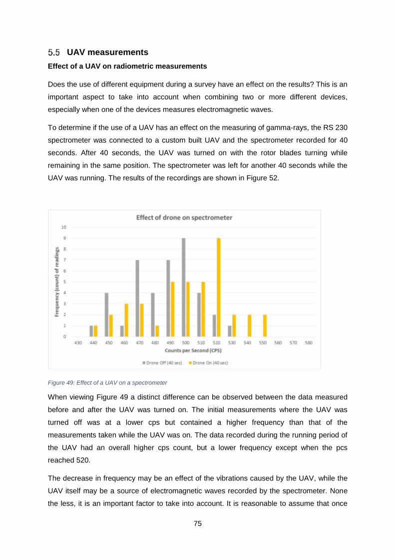
75
UAV measurements
Effect of a UAV on radiometric measurements
Does the use of different equipment during a survey have an effect on the results? This is an
important aspect to take into account when combining two or more different devices,
especially when one of the devices measures electromagnetic waves.
To determine if the use of a UAV has an effect on the measuring of gamma-rays, the RS 230
spectrometer was connected to a custom built UAV and the spectrometer recorded for 40
seconds. After 40 seconds, the UAV was turned on with the rotor blades turning while
remaining in the same position. The spectrometer was left for another 40 seconds while the
UAV was running. The results of the recordings are shown in Figure 52.
Figure 49: Effect of a UAV on a spectrometer
When viewing Figure 49 a distinct difference can be observed between the data measured
before and after the UAV was turned on. The initial measurements where the UAV was
turned off was at a lower cps but contained a higher frequency than that of the
measurements taken while the UAV was on. The data recorded during the running period of
the UAV had an overall higher cps count, but a lower frequency except when the pcs
reached 520.
The decrease in frequency may be an effect of the vibrations caused by the UAV, while the
UAV itself may be a source of electromagnetic waves recorded by the spectrometer. None
the less, it is an important factor to take into account. It is reasonable to assume that once

76
the UAV is running the increased cps will remain constant throughout the survey. Each UAV
may also have a different effect on the data acquired by a spectrometer and has to be
adjusted according to its own effect.
UAV flight
The final UAV system was subjected to strong winds influencing the movement speed as
well as the height correlation. However, despite the environmental factors the UAV finished
the measurements and is represented by Figure 50.
Figure 50: UAV data vs simulated data
The UAV data was compared to a simulation determining the accuracy of the UAV’s
measurements. The yellow line represents the UAVs measurements while the black line
represents the simulation values. Initially, the UAV contained a higher cps value and wasn’t
lined up with the simulation. However, the simulation does not include the effect of the UAV
on radiometric data as well as the influence of strong winds on the positioning of the UAV.
To compensate for the influence of the wind the UAV data was subjected to a 5 point moving
average making the data more relatable to the simulated values.

77
Downscaling
The purpose of UAV measurements is to produce data that is accurate and relatable to
ground measurements. By downscaling the UAV data, we are able to determine if the UAV
measurements can be converted to represent data measured on the ground.
To test the accuracy of downscaling, prior ground measurements need to be available to
compare the results. By altering the H and 𝑛0 value of the height correction equation we can
possibly predict the activity at lower altitudes. The H value needs to represent the distance
between the spectrometer and the ground of the lower altitude, while the 𝑛0value
represents the initial activity value of the higher measured altitude.
𝑛 = 𝑛0𝑒−0.00505∗𝐻
Figure 51 portrays detailed radiometric pole measurements at altitudes of 5, 3, and 1 meter.
The solid lines represent the measured values while dotted lines represent the downscaled
data from five meters to three and one meter.
Figure 51: Downscaling of 5 meter high measurements
Prior to 80 meters the five meter downscaled values convincingly represent the measured
three and one meter values. However, after 80 meters the downscaled values start to drift
away from the actual measurements, indicating a poor correlation. The only difference

78
between the area before and after 80 meters is the activity of the terrain. Prior to the 80
meters readings, the terrain has a homogenous activity with little to no anomalies, but after
80 meters the surface activity values become inconsistent with areas containing a much
higher activity count than the other surrounding areas. Figure 52 illustrates the distribution of
activity over the surface of the tailing dam with each dot representing a 20 meter interval.
The dotted circle indicates the FOV of the spectrometer at an altitude of 5 meters.
Figure 52: New Machavie radioactivity distribution
The FOV is larger at higher altitudes, increasing the amount of anomaly material that is
included than the FOV at lower altitudes, illustrated by Figure 53. Thus, the downscaling
after 80 meters did not take the loss of anomaly detection into account, resulting in an
inaccurate prediction. However, the use of downscaling proved to be an accurate
representation when the area contains a homogenous surface.
Area of higher
radioactivity
Figure 53: Representation of the effect of FOV

79
6 Conclusion and Recommendations
The aim of this study was to determine whether mounting a handheld spectrometer onto a
UAV is a viable solution towards easier and faster radiation data collection. Traditionally
radiometric data is measured by means of a handheld detector operated by a technician
walking survey lines over a test area. The testing method is cheap, but is a time consuming
process and the study area may be unsafe for the operator. Cars or aeroplanes are also
used as alternative radiometric platforms. However, they have restrictions; the use of a car is
faster than walking, but is limited to areas only accessible to vehicles. A confounding factor
is the fact that the vehicle may mask the radiation, resulting in non-accurate readings.
Airborne radiometric surveys are fast and capable of surveying large areas. However, it is a
complex, specialized and extremely costly method (Richards, 1981). Thus, the search for an
alternative surveying method motivated the testing of UAV systems as possible platforms.
UAV systems are faster than walking, more accessible than vehicles and cheaper than
aeroplanes, making them theoretically a great platform for radiometric surveys. Equipping a
UAV with a handheld spectrometer provides a system that is a potential cheap and effective.
The first objective of this study was to determine the detection capabilities of a handheld
spectrometer at different heights above different source sizes. By using the spectrometer’s
field of view (FOV) and a height correction formula, the study proved that the RS 230
spectrometer is capable of accurately measuring gamma rays up to a height of 20 meters.
However, the terrain must be radiologically homogenous. If not homogenous, the measured
data may be misrepresented, due to the influence of radiological hot spots altering the cps
values. The study also proved, by determining the fraction of background (FOB), that an
elevated spectrometer might measure smaller radiological hotspots as background noise. If
the detection of anomalies is important, the spectrometer should be operated at a lower
height.
The second objective was to obtain accurate surface radiometric measurements at different
heights along a predefined survey line. A gold tailings dam was chosen to be used as a
source of radioactive material and a survey line across the tailing dam was identified.
Detailed surveys at different altitudes were conducted, providing valuable data.
Results showed that a handheld spectrometer attached to a stationary UAV is capable of
providing accurate data up to a height of 20 meters. However, in order to complete a survey,
the spectrometer must be able to provide accurate data whilst moving. It became evident
that high speeds had a smoothing effect on the data. When the spectrometer is moving at a

80
slow speed, the measurements are situated close to each other and any variations in
measurements may cause a graph to appear jagged. An area measured at a slow speed
may also overlap with the previously measured area. This can cause alterations especially if
an anomaly is present within the area. If a UAV moves at an increased speed the amount of
overlapping area is decreased, the measurements are also situated further apart giving the
data a smoothed appearance.
It is important to note that the faster a UAV moves, the more the data will be shifted to a
side. If a UAV moves at a speed of four meters per second, then the initial measured count
would have been shifted by roughly four meters. Therefore, it is important for the UAV to
maintain a constant speed throughout the survey and that the data are adjusted accordingly
to represent the correct data at the correct location.
The third objective was to compare the stationary measurements with the UAV surveyed
data. Data obtained by the UAV system differed from that of the reference measurements.
Strong prevailing winds led to the inconsistent flight of the UAV system, which subsequently
influenced the measuring capabilities of the spectrometer. After considering the influence of
the wind on the data, a much stronger correlation with the referenced measurements was
observed.
The last objective was to compare the experimental survey data with the reference ground
survey. The experimental survey data results were downscaled to be compared to the
ground survey. However, certain areas of the tailings dam correctly represented lower
altitude values while other areas misrepresented lower altitude values. The whole test area
was surveyed and indicated areas with elevated cps values or hot spots. The areas that
correctly represented the lower altitude values were homogeneous, containing a constant
cps value. Thus, the downscaling of areas containing hotspots misrepresents the lower
altitude values. The spectrometer’s field of view at higher altitudes included anomalies that
were missed by ground surveys.
Studies exploring the capabilities of UAV technology as an alternative measuring method are
not a new concept. Pirttijärvi & Oy (2016) researched the possibility of a UAV system
replacing walking measurement. However, their findings were solely based on observations
made by generating kriging maps.
This study focused on proving the usability of a UAV system using various mathematical
simulations, and not solely based on visual interpretations. Towler et al, (2012), as well as
Bogatov and Mazny (2013) undertook research studies aimed at using UAV systems during
times of crisis such as the events of Fukushima and Chernobyl. These studies focused on

81
ways of identifying radiological hotspots without putting a human in danger. They did,
however, only focus on identifying hotspots and not on the accuracy of the UAV system.
Previous studies focused on whether it is possible to see a mark on a map, whereas this
study aimed to determine the significance of the mark.
Using a UAV for radiometric measurements may have many positive aspects, but there are
also negative aspects. During the course of the study, three different UAV systems were
used and all three systems were damaged, mostly resulting in incomplete surveys. Thus, a 6
meter PVC pipe was used to mimic a UAV. Appendix 1 contains a fault tree analysis as well
as a critical analysis for each of the failed UAV systems. The system failures included
human error, mechanical damages, depleted power supplies, excessive vibration as well as
miscellaneous failures.
The fault tree analysis identifies the root cause of the failure, while the critical analysis
classifies the failure according to severity, probability and according to the threat of failure.
The severity of the failures varied between critical and catastrophic, while the probability was
less serious only varying between occasional probability and extremely unlikely probability.
Two of the three failures have a moderate threat of failure, while the third one has a low
threat of failure.
Based on simulations and tests, the study proved that the use of an UAV combined with a
spectrometer is a viable alternative for radiometric measurements. A good correlation
between measured and simulated activity values, up to a height of 20 meters, was produced.
The results also presented the effect of speed on measured values and portrayed the effect
of a UAV system on the measuring capabilities of a spectrometer.
The limiting factor of a UAV spectrometer system is the reliability of the UAV itself. The loss
of three UAV systems caused a significant loss of time as well as resources, limiting the
number of tests. Another limiting factor is that some areas contain an inconsistent
distribution of radioactive material. The higher the UAV is situated, the bigger the field of
view will be, resulting in the loss of anomaly values. If a homogenous area is surveyed, the
UAV can measure up to 20 meters in the air, but if the area is inconsistent, the UAV should
remain at an elevation of approximately three meters.
A recommendation for future research into the usability of a UAV system for radiometric
surveys is to include more measurements by using a UAV system that is reliable and cost
effective. The UAV should be able to manage the weight of the detector, while maintaining a
constant height and speed. Ideally, the UAV should also be able to remain airborne for the
whole duration of the survey but if not possible, the tested UAV should require the minimum

82
amount of refueling/recharging. The effects of anomalies on the quality of data should be
further researched. Identifying the optimum height should not solely be based on the size of
the anomaly, but also its radioactive intensity. Finally, the usability of handheld detectors
must be tested at higher altitudes as well as areas with a varying topography.

83
7 References
Alipour, D., Keshtkar, A.R., & Moosavian, M.A. 2016. Adsorption of thorium(IV) from
simulated radioactive solutions using a novel electrospun PVA/TiO2/ZnO nanofiber
adsorbent functionalized with mercapto groups: Study in single and multi-component
systems. Appl. Surf. Sci. Elsevier B.V. 366:19–29.
Allyson, J.D. 1994. Environmental Spectrometry : Simulation of Absolute Calibration of In-
Situ and Airborne Spectrometers for Natural and Anthropogenic Sources by
Submitted to The University of Glasgow for the degree of Doctor of Philosophy
September 1994 This research was c. :1–293.
Anhaeusser, C.R., Johnson, M.R. & Thomas, R.J. 2006. The Geology of South Africa. The
Geological Society of South Africa. Pretoria. ISBN 1-919908-77-3. 691 p
Annandale, E. & Nealer, E. 2011. Exploring aspects of the water history of the
Potchefstroom region and the local management of it. New Contree (Novemer
2011):111–124.
Arazo, M., Barroso, M., Torre, Ó. De, Moreno, L., Ribes, P., Ventura, A., & Orellana-martín,
D. 2016. Uranium- decay chain. Research Group on Natural Computing: 114-130
Aucamp, P. 2003. Trace-element pollution of soils by abandoned gold-mine tailings near
Potchefstroom, South Africa. Bull. Counc. Geosci. (130):1–60.
Beamish, D. 2016. Enhancing the resolution of airborne gamma-ray data using horizontal
gradients. J. Appl. Geophys. Elsevier B.V. 132:75–86.
Bever, N.J. 1997. Proterozoic, auriferous black reef placer in the Transvaal basin
Supervisor : Prof John Moore.
Bogatov, S., Mazny, N., Pugachev, A., Tkachenko, S., Shevdov, A. 2013. Emergency
Radiation Survey Device Onboard the Uav. Int. Arch. Photogramm. Remote Sens.
ans Spat. Inf. Sci. XL-1/W2(September):4–6.
Canadian Nuclear Safety Commission. 2012. Introduction to radiation. British medical
journal. (2):1-38
Coetzee, H. 2008. Acquisition, Processing and Enhancement of Multi- Channel
Radiometric Data Collected With Ultralight Aircraft Mounted Detectors.
Corvisiero, P., Anghinolfi, M., Dzhilavyan, L. z., Gervio, G., Grosso, L., Ricco, G., Sanzone,
M., Taiuti, M., & Zucchiatti, A. 1990. P-14.pdf. Nucl. Instruments Methods Phys.
Res. (A294):478–484.

84
Craton, K., Africa, S., Sumner, D.Y., & Beukes, N.J. 2006. University of California
Postprints Sequence stratigraphic development of the Neoarchean Transvaal
carbonate Sequence stratigraphic development of the Neoarchean Transvaal
carbonate platform , Kaapvaal Craton , South Africa. Africa (Lond). :11–22.
Dasnois, N. 2012. Uranium Mining in Africa: A Continent at the Centre of a Global Nuclear
Renaissance. Gov. Africas Resour. Program. (122):32.
Dirks, P.H.G.M. & Berger, L.R. 2013. Hominin-bearing caves and landscape dynamics in
the Cradle of Humankind, South Africa. J. African Earth Sci. Elsevier Ltd. 78:109–
131.
Erdi-Krausz, G.J., Nicolet, P.N. 2003. Mapping Using Gamma Ray. IAEA: Vienna.
Eriksson, P.G. & Altermann, W. 1998. An overview of the geology of the Transvaal
supergroup dolomites (South Africa). Environ. Geol. 36(1–2):179–188.
Franco, B.J. & Goes, L.C. 2007. Failure Analysis Methods in Unmanned Aerial Vehicle
(UAV) Applications. 19th Int. Congr. Mech. Eng. (November): 5-9
Grasty, R.L. 1979. Gamma ray spectrometric methods in Uranium exploration – theory and
operational procedures, Economic Geology Report 31. p. 147-161, 1979.
Gsenviro. "What is the relationship between altitude and temperature of a place?" eNotes,
27 Nov. 2015, https://www.enotes.com/homework-help/what-relationship-between-
altitude-temperature-556362. Accessed 2 Dec. 2017
Hübsch, T. 1997. The Theory of Alpha Decay. Uranium. (Term paper. Howard University,
Washington)
Kamunda, C., Mathuthu, M., & Madhuku, M. 2016. An Assessment of Radiological Hazards
from Gold Mine Tailings in the Province of Gauteng in South Africa. Int. J. Environ.
Res. Public Health. 13(1):138.
Killeen, P.G. 1979. Gamma-ray spectrometric methods in uranium exploration - application
and interpretation. Geophys. Geochemistry Search Met. Ores. :163–230.
Knoll, G.E. & Wiley, J. 2000. Radiation Detection and Measurement Third Edition. John
Wiley & Sons, Inc
Koch, J. 2014. Miugration of gamma ray assessment of uranium on a gold tailings disposal
facility. Potchsefstroom: NWU. (Thesis – MSc)
85
Lawson, R. 1999. An Introduction to Radioactivity by. An Introd. to Radioact. (October
1999):1–20.
Lawson, R.S. 2013. Practical SPECT/CT in Nuclear Medicine. :19–34.
Loveland, W., Morrissey, D.J., & Seaborg, G.T. 2006. Beta Decay. , Modern Nuclear
Chemistry.
Melorose, J., Perroy, R., & Careas, S. 2015. No Title No Title. Statew. Agric. L. Use
Baseline 2015. 1.
Minty, B.R.S. 1997. Fundamentals of airborne gamma-ray spectrometry. AGSO J. Aust.
Geol. Geophys. 17(2):39–50.
Murray, R.L. & Holbert, K.E. 2015. Chapter 3 - Radioactivity. Nucl. Energy (Seventh Ed.
:31–46.
Pirttijärvi, M. & Oy, R. 2016. Radai’s UAV based radiometric measurements at Rautuvaara
mine in Kolari. (Report, radai)
Pöllänen, R., Toivonen, H., Peräjärvi, K., Karhunen, T., Ilander, T., Lehtinen, J., Rintala, K.,
Katajainen, T., Niemelä, J., & Juusela, M. 2009. Radiation surveillance using an
unmanned aerial vehicle. Appl. Radiat. Isot. 67(2):340–344.
Poole, C.P. 2004. Encyclopedic dictionary of condensed matter physics: Volume 1 A-M.
Richards, D.J. 1981. Geophysical field manual for technicians. South African geophysical
association No. 2.
Schröder, S., Lacassie, J.P., & Beukes, N.J. 2006. Stratigraphic and geochemical
framework of the Agouron drill cores, Transvaal Supergroup (Neoarchean-
Paleoproterozoic, South Africa). South African J. Geol. 109(1–2):23–54.
Summer, D.Y. & Beukes, N.J. 2006. Sequence stratigraphic development of the
Neoarchean Transvaal carbonate platform. South African Journal of Geology.
109:11–22.
Towler, J., Krawiec, B., & Kochersberger, K. 2012. Terrain and radiation mapping in post-
disaster environments using an autonomous helicopter. Remote Sens. 4(7):1995–
2015.
Wendel, G. 1998. Radioactivity in mines and mine water — sources and mechanisms A
Curie of Rock. Most. (April):87–92.

86
Wright, V.P. & Burchette, T.P. 1998. Carbonate ramps: an introduction. Geological Society
of London. 149:1–5.

87
8 Appendix
List of Figures
Figure 1: Complete fault tree analysis (Franco et al, 2007) ................................................. 89
Figure 2: Fault tree analysis (Loss of propeller) ................................................................... 91
Figure 3: Fault tree analysis (Human Failure) ..................................................................... 95
Figure 4: Fault tree analysis (Fuel system failure) ............................................................... 96
List of Tables
Table 1: Failure severity classification (Franco et al, 2007) ................................................. 90
Table 2: Failure occurrence probability (Franco et al, 2007) ................................................ 90
Table 3: Failure severity analysis (Gyrolag) ........................................................................ 92
Table 4: Failure occurrence probability (Gyrolag) ................................................................ 92
Table 5: Estimating future threat (Gyrolag) .......................................................................... 93
Table 6: Failure severity calssification (Haevic drones) ....................................................... 97
Table 7: Failure occurrence probability (Haevic drones) ...................................................... 97
Table 8: Threat of Failure (Haevic drones) .......................................................................... 98
Table 9: Failure severity classification (UAV industries) .................................................... 100
Table 10: Failure occurrence probability (UAV industries) ................................................. 100
Table 11: Threat of failure (UAV industries) ...................................................................... 101

88
Method assessment
8.1.1 Introduction
During the research study, a number of incidents took place regarding the performance of
different UAV systems providing merit for the use of objective as well as subjective
assessments on the reliability and usability of UAV systems in the commercial market. The
reliability of UAVs is influenced by a wide range of environmental, human and mechanical
factors contributing or prohibiting to the performance of a UAV during field tests. Franco and
Goes defines UAV reliability as “the probability that a UAV will operate without failure for the
duration (t) of a specified mission profile, given that it was fully operation at the time (t=0), as
well as during in preflight tests.”
When a UAV is compared to a manned aircraft, it is desired that the UAV will be a more
cost-effective substitute while still providing services that are at an acceptable level for the
research mission. These services include the level of safety, operability, mission reliability
and survivability (Franco & Goes, 2007).
During the project a total of three UAVs had been used to obtain the required data, all three
of the drones sustained damage during the test period. The complications took place at
different stages of the flight and varied from mechanical, human, environmental, product
limitations and miscellaneous errors.
Initial background information will be provided explaining the circumstances for each case
study including the capability of the operator, mechanical reliability, UAV limitations,
miscellaneous occurrences, and the environmental factors. After the background information
has been established a Fault Tree Analysis (FTA) will be conducted identifying the cause of
the failed attempt. Finally, a Critical Analysis (CA) will be performed to determine the
probability of the mishap occurring again in the future.
A fault tree analysis (FTA) is a safety design analysis that is used to represent a failure or
combination of failures as a graphical representation. The analysis starts by identifying the
“top events” of the failure referring to the effects of the system failure. The analysis proceeds
by determining how the top event can be caused by a single or combination of lower level
failures according to a known set of failure modes. The fault tree analysis functions on the
logical interactions between different systems and how the fault of one or a combination of
systems can affect the product as a whole. Figure 1 depicts the complete fault tree system
with the top event as the loss of propulsion and from there the tree branches out and
becomes more specific as it moves down towards lower level failures.

89
Figure 1: Complete fault tree analysis (Franco et al, 2007)
A critical analysis will rank the failure of the UAV by the probability of it happening again as
well as the effect that the failure had on the mission and the UAV.
Loss of Propulsion
OR
Human failure Loss of Propeller Loss of Engine
Structural Failure Propeller stops abruptly
Connection Failure
Engine failure
Engine control Failure
Mechanical Failure
Lubrification System Failure
Fuel Improper
Fire
Engine failure
Induction system Engine Control Failure
Fuel System Failure
OR OR
OR OR

90
Table 1: Failure severity classification (Franco et al, 2007)
Category Description Mishap Definition
1 Catastrophic A failure which may cause system of UAV Platform loss
2 Critical A failure which may cause major system damage which will
result in a UAV mission loss
3 Marginal A failure which may cause minor system damage which will
result in a delay or loss of availability or mission degradation.
4 Minor A failure not serious enough to cause system damage, but
which will result in unscheduled maintenance or repair.
Table 1 classifies the effect that the failure may have on the mission as well as the UAV,
whereas table 2 ranks the failure according to the probability of it happening again.
Table 2: Failure occurrence probability (Franco et al, 2007)
Level Occurrence Probability
A Frequent 0>0.2
B Reasonable probability 0.10>0>0.2
C Occasional probability 0.01>0>0.1
D Remote probability 0.001>0>0.1
E Extremely unlikely probability 0<0.001
8.1.2 Gyrolag: Infotron IT 180
The geophysics company Gyrolag provided the University with an Infotron IT 180 UAV with
the goal to research the usability of drones in the commercial market. The UAV was initially
designed for military operations and has been used by the French army since 2012. The
UAV is powered by a gasoline engine capable of flying with a 3+ kg payload for 25 minutes.
The UAV operator is a licensed pilot with vast knowledge regarding the rules and regulations
of aerospace. Safety is a priority for the company and they ensured that all safety equipment
and procedures were followed. The UAV flight plan was preemptively installed onto the

91
ground control station (GCS) and had the necessary emergency protocols to react to an
unforeseen complication.
The preflight didn’t indicate any malfunctions and the go-ahead was given. But during the
startup, the UAV began to shake uncontrollably and forced the pilot to push the fail switch to
disable the UAV. After the UAV came to rest, a quick inspection revealed that a mechanical
breakage occurred at one of the blade’s angle stabilizers. The stabilizer broke off and
damaged some of the rotor blades, making the UAV unstable resulting in the UAV shaking
uncontrollably further damaging the internal structures.
Fault tree (Gyrolag)
The damaged internal structure was a result of excessive vibrations and is categorized as a
mechanical failure. However, the excessive vibrations were a result of the rotor blade
stabilizers breaking off and damaging the blades making the UAV unstable. The instability of
the UAV caused the excessive vibrations damaging the structure. Thus the damage caused
to the UAV structure is a combination of mechanical and rotor failure, but the initial damage
to the propeller instigated a chain reaction (figure 2).
Figure 254: Fault tree analysis (Loss of propeller)
Connection Failure
OR
Propeller stops abruptly Structural Failure
Loss of Propeller

92
Critical analysis (Gyrolag)
The mechanical failure resulted in significant system damage, grounding the UAV and
prohibiting any further measurements. Based on the criteria from the failure severity
classification system the mechanical failure is categorized as second degree as seen in
table 3.
Table 3: Failure severity analysis (Gyrolag)
Category Description Mishap Definition
1 Catastrophic A failure which may cause System of UAV Platform loss
2 Critical A failure which may cause major system damage which will
result in a UAV mission loss
3 Marginal A failure which may cause minor system damage which will
result in a delay or loss of availability or mission degradation.
4 Minor A failure not serious enough to cause system damage, but
which will result in unscheduled maintenance or repair.
Mechanical failure is a part of normal wear and will happen throughout the UAV’s operating
lifespan. The quality of the UAV’s production will affect the amount of normal wear that will
occur and influence the time intervals between the failures. Due to the complexity and quality
of the UAV’s production, it will be expected that normal wear will occur occasionally as seen
in table 4.
Table 47: Failure occurrence probability (Gyrolag)
Level Occurrence Probability
A Frequent 0>0.2
B Reasonable probability 0.10>0>0.2
C Occasional probability 0.01>0>0.1
D Remote probability 0.001>0>0.1
E Extremely unlikely probability 0<0.001
After cross referencing the classification from table 3 and 4 and plotting it onto table 5.Table

93
Table 58: Estimating future threat (Gyrolag)
Level A
Frequent
CRITICAL
Level B
Reasonably
probable
Level C
Occasional
Level D
Remote
Level E
Extremely
unlikely
LOW
Category 4
Minor
Category 3
Marginal
Category 2
Critical
Category 1
Catastrophic
Based on table 1 we can estimate that the mechanical failure poses a moderate threat to
future UAV operations. A possible solution to limit the occurrence or damages as a result of
mechanical failures is regular maintenance, diligent preflight checks, using high-quality UAV
systems, skilled operators and correct emergency protocol.

94
8.1.3 Haevic Drones
After Gyrolag’s UAV failure, a new drone was required to finish the radiometric
measurements. Haevic drones, a side branch company of Triomf, was approached to work
in collaboration with the university to complete the radiometric measurements. The drone
that was suggested for the test was a custom built six blade UAV. The UAV was previously
used for distributing agricultural pesticides and is capable of carrying 5 kg. The UAV is
battery powered and can fly with a payload for 10 minutes.
The flight plan was established and developed a few days before the mission flight. Safety
precautions were a priority, and all necessary gear was present the day of the flight. Before
the flight commenced, a preflight check was conducted and the go-ahead was given. After
the UAV took flight, it proceeded to move towards the initial test line. The initial speed of the
UAV was at a startling slow pace. A few minutes later, the UAV signaled red indicating that
the battery has been depleted. Shortly after the initial warning, the UAV started to lose
altitude at an increasing rate. The UAV made contact with the ground, breaking off two of the
rotor limbs and damaged the UAV’s framework. When the UAV crashed the RS 230
spectrometer broke loose from its frame hitting the ground and damaged the casing, but no
internal damage resulted.
There were no immediate explanations for why the UAV crashed, but after further
investigations, two possible factors were suggested that might have contributed to the crash.
Firstly the flight plan that was inserted into the computer was incomplete. It didn’t specify the
speed at which the UAV should initially move towards the starting point resulting in the slow
hovering UAV losing battery life as it went on. Although the battery charge time is
supposedly 10 minutes, the operator suggested that the weight of the payload may have
influenced the flight time. As previously mentioned the drone is said to be able to carry 5 kg,
but the difference being from a fixed payload the 5 kg payload becomes lighter over time
once the distribution of pesticides has started. Thus, a fixed weight payload might have
shortened the expected flight time and together with the loss of initial battery life could have
been enough to cause a crash.

95
Fault tree (Haevic Drones)
The Haevic drones mission failure was a result of inadequate procedure planning as well as
loss of battery power. The insufficient knowledge regarding the correct insertion of a mission
plan contributed to energy wasted on positioning. The weight of the spectrometer could also
have influenced the battery life, as previously mentioned the operator suggested that the
fixed weight of the spectrometer could have influenced the rapid depletion of the UAV’s
batteries. Based on the fault tree analysis the inadequate procedure planning falls under the
Human Failure fault tree (figure 3) whereas the insufficient battery power is identified as Fuel
Depletion under the fuel system failure as seen in figure 4 (The fault tree is developed for
fuel powered UAV’s, but can be slightly altered for battery-powered UAV systems).
Figure 3: Fault tree analysis (Human Failure)
Human Failure
Wrong Reaction
To Failure
Excessive Workload
Fatigue
Ergonomics
Inadequate
Training
Inadequate
MMI
Misjudgement
(Weather)
Inadequate
Procedures
OR

96
Figure 4: Fault tree analysis (Fuel system failure)
Critical analysis (Haevic Drones)
The UAV failure caused catastrophic system damage to its systems, resulting in a complete
termination of any further measurements. Based on the criteria from the failure severity
classification system the mechanical failure is categorized as a first degree catastrophe as
seen in table 6.
Fuel System Failure
Loss of Fuel
Supply
Failure of Engine
Fuel System
Fire / Explosion
Fuel Depleted
Penetration of Fuel Lines
Penetration of Fuel Tank
Hydrodynamic Ram
Fuel Tank Line Failure Fuel pump Line Failure
Fuel pump Failure
Fire
Carburettor Failure

97
Table 69: Failure severity calssification (Haevic drones)
Category Description Mishap Definition
1 Catastrophic A failure which may cause System or UAV Platform loss
2 Critical A failure which may cause major system damage which will
result in a UAV mission loss
3 Marginal A failure which may cause minor system damage which will
result in a delay or loss of availability or mission degradation.
4 Minor A failure not serious enough to cause system damage, but
which will result in unscheduled maintenance or repair.
Human error can occur in every study where direct interaction is needed influencing the
results of a product or study. The possibility of a human error occurring at a company is
dependent on the capability and experience of the people working for the company. It is
difficult to estimate the chance of it happening again when only taking a few companies into
account. But when reviewing the overall capability of the companies worked with in this
study, it can be assumed to happen only rerely. For Haevic Drones the study was a new
experience for the company increasing the likelihood for something to go wrong.
Due to the UAV being custom built meant that the manufactures didn’t have to test the
product to determine its maximum capabilities. Thus, the probability of a custom-built UAV to
be inadequate to successfully finish is greater than a UAV that is regulated by the market.
The probability of a failure happening again is based on the competency of the company and
as previously mentioned the overall capability of the companies worked with was
outstanding, making it a rare occurrence (table 7).
Table 7: Failure occurrence probability (Haevic drones)
Level Occurrence Probability
A Frequent 0>0.2
B Reasonable probability 0.10>0>0.2
C Occasional probability 0.01>0>0.1
D Remote probability 0.001>0>0.1
E Extremely unlikely probability 0<0.001
When plotting the plausibility over the severity of the failure, we can estimate the threat of
failure. Although the failure led to catastrophic damage to the UAV making it unusable for

98
any further studies it was due to a rare chance of human error as well as faulty design
making it less of a threat.
Table 8: Threat of Failure (Haevic Drones)
Level A
Frequent CRITICAL
Level B
Reasonably
probable
Level C
Occasional
Level D
Remote
Level E
Extremely
unlikely
LOW
Category 4
Minor
Category 3
Marginal
Category 2
Critical
Category 1
Catastrophic
When reviewing the threat of failure table (table 8), we can estimate the specific failures to
be a moderate threat towards UAV flight missions. Thus, it is of the utmost importance that
any company that works with UAVs is familiar with all of the different components that may
influence the UAV’s flight path or the success of the flight mission. This includes the physical
capabilities of the UAV, the UAV’s software system as well as the competency of the pilot or
operator.
8.1.4 UAV industries
With limited useable data due to multiple failed UAV attempts, a third company was
approached to finish the flight mission. UAV industries a professional UAV company based
in Cape Town was contracted to continue the measurements at New Machavie. The
company specializes in videography for movies and sports events but was eager to broaden
its capabilities to accommodate research studies. The drone that was proposed for the study

99
was a custom-built octocopter and was previously used to carry camera equipment that
weighs up to six kg being more than capable of transporting the RS 230 spectrometer.
The flight planning entailed a detailed flight path developed using google earth, establishing
the aims and objectives of the study, and requesting permission from the mine as well as the
army due to the testing area being within the field-testing radius of the army. UAV industries
send two employees for the field-testing of whom one was the operator and the other the
manager. Before the flight, the landing zone was identified, and a temporary base station
was established. The UAV was assembled and moved towards the landing zone where
numerous preflight checks were conducted. Just before takeoff, a warning was broadcast on
the radio to any aeroplanes within the vicinity of the testing site. After takeoff, the UAV
struggled to obtain a connection with satellites due to the fast prevailing wind speeds
pushing the UAV off course. After numerous failed attempts, the operator decided to fly the
UAV by hand at an altitude of five meters above the tailing dam. Due to the prevailing winds,
the first flight attempt by hand proved to be too difficult causing the UAV to vary its altitude
during the flight resulting in inconsistent data.
The drone eventually established a GPS connection and was able to finish the first mission
flight at an altitude of five meters. The second test required the UAV to fly horizontal lines at
an altitude of 5 meter over the tailingdam. The total distance for the survey proved to be too
long for the UAV to fly it on one set of batteries. After the first battery change, the UAV had
to established a GPS connection and started to continue with the survey. However, as soon
as the UAV began with the survey it flipped upside down and crashed into the tailing dam.
The crash caused two rotor limbs to break off as well as major structural damage to the
frame and hardware. The test was cancelled, and no further data was obtained.
Directly after the crash both UAV industry employees tried to determine the cause of failure,
but with no success.
Fault tree analysis (UAV industries)
Due to the uncertainty of the crash, it is difficult to assign a cause to the failure. The purpose
of the fault tree analysis is to establish the cause so that it can be used to prevent future
failures. Unfortunately, there is no miscellaneous or unknown category within the fault tree
system. Therefore this specific failure cannot be categorized according to it.

100
Critical analysis (UAV industries)
The crash resulted in catastrophic damage rendering the UAV useless. On the severity of
failure table, it is classified as catastrophic due to mayor system damage (table 9).
Table 9: Failure severity classification (UAV industries)
Category Description Mishap Definition
1 Catastrophic A failure which may cause System or UAV Platform loss
2 Critical A failure which may cause major system damage which will
result in a UAV mission loss
3 Marginal A failure which may cause minor system damage which will
result in a delay or loss of availability or mission degradation.
4 Minor A failure not serious enough to cause system damage, but
which will result in unscheduled maintenance or repair.
Due to the uncertainty of the crash, it is difficult to confidently classify the plausibility of it
happening again in the future. According to the UAV operator, he has never experienced the
specific failure before and had no idea what caused the failure. Thus, based on the
operator's experience and the unknown cause of the failure the plausibility is classified as a
level E (table 10).
Table 10: Failure occurrence probability (UAV industries)
Level Occurrence Probability
A Frequent 0>0.2
B Reasonable probability 0.10>0>0.2
C Occasional probability 0.01>0>0.1
D Remote probability 0.001>0>0.1
E Extremely unlikely probability 0<0.001
After plotting UAV industries product failure of plausibility over the severity on the threat of
failure table (table 11), we can deduce that the crash was an extremely unlikely event that
caused catastrophic damage to the UAV system. Although the damages to the system were
severe, the unusual likelihood of the failure happening again classifies the failure as a low
threat of failure.

101
Table 11: Threat of failure (UAV industries)
Level A
Frequent
CRITICAL
Level B
Reasonably
probable
Level C
Occasional
Level D
Remote
Level E
Extremely
unlikely
LOW
Category 4
Minor
Category 3
Marginal
Category 2
Critical
Category 1
Catastrophic