lbm 2008 (cla 2008) · 2008-10-11 · palacky´ university, olomouc, czech republic lattice-based...

LBM 2008 (CLA 2008)Proceedings of the Lattice-Based Modeling Workshop, in conjunction withThe Sixth International Conference on Concept Lattices and Their Applications

Palacky University, Olomouc, Czech Republic

ISBN 978–80–244–2112–4

Palacky University, Olomouc, Czech Republic

Lattice-Based Modeling Workshop

LBM 2008

Olomouc, Czech RepublicOctober 21–22, 2008

CLA 2008The Sixth International Conference on

Concept Lattices and Their Applications

Edited by

Vassilis KaburlasosUta Priss

Manuel Grana

LBM 2008 (CLA 2008)c© Vassilis Kaburlasos, Uta Priss, Manuel Grana, Editors

This work is subject to copyright. All rights reserved. Reproduction or publica-tion of this material, even partial, is allowed only with the editors’ permission.

Technical Editor:Jan Outrata, [email protected]

Page count: x+67Impression: 70Edition: 1st

First published: 2008

Published and printed by:Palacky University, Olomouc, Czech Republic

Organization

LBM 2008 was organized in conjunction with CLA 2008 by the Palacky Univer-sity, Olomouc, and the State University of New York at Binghamton.

CLA 2008 General Chairs

Radim Belohlavek State University of New York at Binghamton, USASergei O. Kuznetsov State University Higher School of Economics, Moscow,

Russia

Program Chairs

Vassilis Kaburlasos Technological Educational Institution of Kavala, GreeceUta Priss Napier University, Edinburgh, United KingdomManuel Grana Universidad del Pais Vasco, San Sebastian, Spain

Program Committee

Manuel Grana Universidad del Pais Vasco, San Sebastian, SpainAnestis Hatzimichailidis Technological Educational Institution of Kavala, GreeceVassilis Kaburlasos Technological Educational Institution of Kavala, GreeceEtienne Kerre Ghent University, BelgiumJun Liu University of Ulster, Northern Ireland, United KingdomStelios Papadakis Technological Educational Institution of Kavala, GreeceUta Priss Napier University, Edinburgh, United KingdomGerhard Ritter University of Florida, Gainesville, USAPeter Sussner State University of Campinas, BrasilGonzalo Urcid National Institute of Astrophysics, Optics, and Elec-

tronics; Puebla, MexicoIvan Villaverde Universidad del Pais Vasco, San Sebastian, SpainYang Xu Southwest Jiaotong University, Chengdu, Sichuan,

China

Organization Committee

Michal Krupka (Chair) Palacky University, Olomouc, Czech RepublicEduard Bartl State University of New York at Binghamton, USAJan Konecny State University of New York at Binghamton, USATomas Kuhr Palacky University, Olomouc, Czech RepublicPetr Osicka Palacky University, Olomouc, Czech RepublicJan Outrata Palacky University, Olomouc, Czech Republic

Sponsoring Institutions

PIKE ELECTRONIC, Czech Republic – main sponsor

PIKE Electronic is one of the leading Central European IT companies providingcomplex service in the field of software application development. The Companydelivers or participates on large-scale projects around the globe, cooperating withpartners such as Siemens AG, Siemens E&A, SMS DEMAG, TIBCO, Hewlett–Packard, Accenture or Oracle. The main strategic target is specialization in “corebusiness” areas, consolidation, effective distribution and use of long-term expe-riences and know-how in segments of Process Automation, SOA & EnterpriseApplication Integration , Information Systems for Health Insurance, BusinessIntelligence, Telecommunication, Banking, and Logistic.PIKE ELECTRONIC and the Department of Computer Science of Palacky Uni-versity have been cooperating for more than ten years. In the recent years, PIKEELECTRONIC participated in a large research project on Relational Data Anal-ysis which was supported by the Academy of Sciences of the Czech Republicduring 2004–2008. The principal investigator was Professor Radim Belohlavekfrom the Department of Computer Science, the principal co-investigator was Dr.Stanislav Opichal from PIKE. The research results of this project were publishedin premier international journals and in proceedings of recognized internationalconferences.

SwissCentrum software, Czech Republic

Faculty of Science, Palacky University, Czech Republic

Table of Contents

Preface

Papers

Lattice-based Modelling of Thesauri . . . . . . . . . . . . . . . . . . . . . . . . . . . . . . . . . 1Uta Priss, L. John Old

Piecewise-Linear Approximation of Nonlinear Models Based on IntervalNumbers (INs) . . . . . . . . . . . . . . . . . . . . . . . . . . . . . . . . . . . . . . . . . . . . . . . . . . . 13

Vassilis G. Kaburlasos, S. E. Papadakis

Computation of a Sufficient Condition for System Input Redundancy . . . . 23S. E. Papadakis, V. G. Kaburlasos

An Approach from Lattice Computing to fMRI Analysis . . . . . . . . . . . . . . . 33Manuel Grana, Maite Garcıa-Sebastian, Ivan Villaverde, ElsaFernandez

Redundant Encoding of Patterns in Lattice Associative Memories . . . . . . . 45Gonzalo Urcid, Gerhard X. Ritter, Jose-Angel Nieves-V.

A Novel Fuzzy Implication Stemming from a Fuzzy Lattice InclusionMeasure . . . . . . . . . . . . . . . . . . . . . . . . . . . . . . . . . . . . . . . . . . . . . . . . . . . . . . . . . 59

Anestis G. Hatzimichailidis, Vassilis G. Kaburlasos

Author Index . . . . . . . . . . . . . . . . . . . . . . . . . . . . . . . . . . . . . . . . . . . . . . . . 67

Preface

With the proliferation of computers, a variety of domain-specific informationprocessing paradigms have emerged. The corresponding analysis- and design-tools (of mathematical nature) are largely disparate due to the need to cope withdisparate types of data including logic values, (fuzzy) numbers/sets, symbols,graphs, etc. A unification of the aforementioned tools is expected to result in auseful technology cross-fertilization. Nevertheless, an “enabling” mathematicalframework is currently missing.It turns out that popular types of data, including the aforementioned ones, arelattice-ordered. Hence, lattice theory (LT) emerges as a promising “enabling”mathematical framework; furthermore, Lattice Computing (LC) emerges as thecorresponding information processing paradigm. In contrast to typical informa-tion processing, which carries out “number crunching” techniques in space RN ,an additional advantage of LC is its capacity to carry out semantic computing.There is a number of isolated research communities, or Communities for short,which employ LT in various information processing domains including 1) Logicand Reasoning, for automated decision-making [5], 2) Mathematical Morphology,for signal- and imageprocessing [4], 3) Formal Concept Analysis, for knowledge-representation and information retrieval [1], 4) Computational Intelligence, forclustering, classification, and regression [2]. However, despite a creative interac-tion within a Community, different Communities typically work separately [3].Hence, practitioners of LT typically develop their own tools/practices withoutbeing aware of valuable contributions by colleagues in other Communities. Inconclusion, potentially useful work may be ignored or duplicated.This workshop is an initiative towards a creative interaction/integration. Sixpapers are presented in this volume. The first one is a review paper, whereas theremaining ones present original (preliminary, though) research results in differentdomains of interest as explained in the following.The paper by Priss and Old revisits ideas on lattices as underlying conceptualstructures in information retrieval and machine translation applications.The paper by Kaburlasos and Papadakis presents techniques for piecewise-linearapproximation of nonlinear models based on Interval Numbers (INs).The paper by Papadakis and Kaburlasos introduces a technique for input vari-able selection based on lattice-ordered Interval Numbers (INs).The paper by Grana, Garcıa-Sebastian, Villaverde, and Fernandez introducesan approach to fMRI (image) analysis based on the lattice associative memory(LAM) endmember induction heuristic algorithm (EIHA).The paper by Urcid, Ritter, and Nieves-Vazquez presents lattice-associativememories able to recall (image) patterns degraded by mixed or random noise.Finally, the paper by Hatzimichailidis and Kaburlasos introduces a fuzzy impli-cation stemming from a fuzzy lattice inclusion measure.

Vassilis Kaburlasos [email protected] Priss [email protected] Grana [email protected]

Chairs, Lattice-Based Modeling (LBM 2008) Workshopin the context of

The Sixth Intl. Conf. on Concept Lattices and Their Applications (CLA 2008)21–23 October 2008, Olomouc, Czech Republic

References

1. B. Ganter, R. Wille, Formal Concept Analysis. Berlin, Germany: Springer, 1999.2. V.G. Kaburlasos, Towards a Unified Modeling and Knowledge-Representation

Based on Lattice Theory. Berlin, Germany: Springer, Studies in ComputationalIntelligence 27, 2006.

3. V.G. Kaburlasos, G.X. Ritter (eds.), Computational Intelligence Based on LatticeTheory. Berlin, Germany: Springer, Studies in Computational Intelligence 67, 2007.

4. G.X. Ritter, J.N. Wilson, Handbook of Computer Vision Algorithms in ImageAlgebra, 2nd ed. Boca Raton, FL: CRC Press, 2000.

5. Y. Xu, D. Ruan, K. Qin, J. Liu, Lattice-Valued Logic. Heidelberg, Germany:Springer, Studies in Fuzziness and Soft Computing 132, 2003.

Lattice-based Modelling of Thesauri

Uta Priss and L. John Old

Napier University, School of Computingu.priss,[email protected]

Abstract. This paper revisits ideas about the use of lattices as under-lying conceptual structures in information retrieval and machine trans-lation as suggested by researchers in the 1950s and 1960s. It describeshow these ideas were originally presented, how they are related to eachother and how they are represented in modern research, particularly withrespect to Formal Concept Analysis.

Key words: Lattice-based modelling, thesauri, machine translation, in-formation retrieval

1 Introduction

Over the past 20 years, Formal Concept Analysis1 (FCA) has gained interna-tional recognition with respect to its applications of lattice theory to fields suchas knowledge representation, information retrieval and linguistics. But there havealso been other non-FCA applications of lattice theory in the same areas. Someof these are very similar to FCA applications in that they also emphasise a dual-ity between two sets (what FCA calls “formal objects” and “formal attributes”)which forms a Galois connection. Other non-FCA applications use only the lat-tice operations, but do not emphasise the Galois connection. For this paper weinvestigate two historic (1950-60s), non-FCA applications of lattice theory tothe area of semantic structures, modelled using thesauri. In particular, we areinterested in the impact that these developments had: is modern research in thisarea a continuation or just a repetition of ideas that were suggested 40-50 yearsago? Do these old research papers still inspire modern work, or have the immenseimprovements in hardware and software made the old research obsolete?

The two research areas we are considering are the work by Margaret Mas-terman as the founder of the Cambridge Language Research Unit in the area of“mechanical translation” and the lattice-based retrieval model by Mooers andSalton that was proposed in Salton’s (1968) influential textbook on informationretrieval. Masterman et al. (1959) argue that both fields are part of a more gen-eral field of “semantic transformation” because mechanical translation uses athesaurus as a retrieval tool in a similar manner to how thesauri are used as aninterlingua in information retrieval. In modern terminology such a field might be

1This paper is not an introduction to FCA. Such an introduction can be found inGanter and Wille (1999) or via the bibliography at http://www.fcahome.org.uk.

c© Vassilis Kaburlasos, Uta Priss, Manuel Grana (Eds.): LBM 2008 (CLA 2008),pp. 1–12, ISBN 978–80–244–2112–4, Palacky University, Olomouc, 2008.

called “conceptual structures” and would contain a range of formal structures(class hierarchies, ontologies, conceptual graphs), not just thesauri.

Both groups of researchers selected for this paper have had a tremendous im-pact on the development of their respective fields (natural language processingand information retrieval). But although the fields have grown, it seems to usthat the use of lattice theory in these fields has not grown to the same degreeand some of the original ideas appear lost in later work. While there is some useof lattices in modern information retrieval, most modern retrieval applicationsuse the vector space model (which was also described by Salton (1968)) insteadof the lattice model. Most modern natural language processing uses statisticaland other non-lattice methods. Nevertheless there are a few modern lattice ap-plications in these areas which are promising. Thus, it may be useful to revisitthe old ideas.

The lattice-based applications we are interested in are not predominantlyBoolean lattices. Many researchers have observed that Boolean lattices form atheoretical basis for information retrieval because the set of all possible subsetsof documents or the set of all possible subsets of keywords form Boolean lattices.The elements of a Boolean logic or Boolean algebra also form a Boolean lattice.Thus, any computer program that uses 0’s and 1’s and AND, OR and NOToperates on Boolean lattices. Even the ancient Chinese book, the I Ching, with its64 trigrams each consisting of 6 lines that can either be broken (i.e. correspondingto 0) or solid (i.e. corresponding to 1), describes a Boolean lattice with 26 = 64elements. Leibniz’s representation of “primitive concepts by prime numbers andcompound concepts by products of primes” (Sowa, 2006) in the 17th centuryis another Boolean lattice. Unfortunately, forming such Boolean lattices doesnot yield much information. In Leibniz’s example, each possible combinationof different prime numbers yields another element of the lattice. The I Chingcontains every possible combination of a 6 character string of 0’s and 1’s. Thisis equivalent to forming every possible subset of a set with 6 elements. Thus,Boolean lattices occur in many situations but in each case they only list allpossible combinations of a certain kind. In information retrieval applications, aBoolean lattice of query terms (or keywords) simply records the fact that everyset of query terms can be formed. In Masterman’s idea of using lattices as aninterlingua for translating between languages, a Boolean lattice represents everypossible combination of words.

In order to illustrate how such Boolean lattices can be visualised, an exampleusing Docco 2 is shown in Fig. 1. Docco is an FCA-based tool that indexes fileson a computer. In the example in Fig. 1, Docco was used to index a directorywith email folders. The folders serve as the formal objects of the concept lattice.Their counts are displayed below the nodes representing the formal concepts. Theformal attributes are terms entered into the search field. An attribute belongsto an object if the term occurs in any of the emails in that folder. The attributenames are displayed slightly above the nodes to which they belong. In this casea search for “meeting Friday project student” was submitted. A Boolean lattice

2http://tockit.sourceforge.net/docco

2 Uta Priss, L. John Old

with four atoms is automatically drawn by Docco in response to the four searchterms. Each concept in the lattice corresponds to a combination of the searchterms. For example, the first node that can be reached by travelling down from“meeting” and “Friday” has three formal objects. Fig. 1 demonstrates how, afterclicking on that concept, the result of a more narrow query, “meeting and Friday”within the broader query, is shown. The file hierarchy on the right is expandedto show the names of the three email folders which contain both the words“meeting” and “Friday”, but not “project” or “student”. In this case there is afolder with the name “studentproject”, which is quite likely relevant to the query.Coincidentally, the emails in the studentproject folder do not themselves containthe words “project” and “student”, but this can happen. The nodes below andabove this concept are also highlighted in the diagram because quite often, ifusers do not find an exact match, slightly expanding or restricting a query willshow relevant results. The idea for using a lattice representation instead of alisting of the results, is so that users obtain feedback on the structure of theresult set.

Boolean lattices easily become too large to be represented graphically. UsingDocco, it would be difficult to visualise searches with more than five or six terms,but most users probably only use two or three terms for these kinds of searchesanyway. A Boolean lattice with n atoms contains 2n elements. Thus, unless theapplication domain is very small, it is not practical to graphically represent theBoolean lattice and to plot actually occurring combinations on it. From an in-formation theoretic viewpoint, lattices that are not Boolean are usually muchmore interesting because they contain information about which elements can-not be combined with which other elements, or which combinations of elementsmight imply other combinations of elements. Thus, while Boolean lattices are oftheoretical value for describing, for example, query languages and interlinguas,for many applications, smaller, non-Boolean lattices or substructures of latticesare more interesting. Methods that extract such smaller lattices or substructuresare of importance. This might be an explanation for why there was an initialenthusiasm about lattices in information retrieval and natural language process-ing: initially, it was discovered that Boolean lattices are of relevance in bothdomains. But until methods were developed that focused on extracting smallersubstructures (as is achieved by FCA methods), the interest in lattices subsided.

The remainder of this paper is organised as follows: Section 2 describes thelattice model of information retrieval as described by Mooers and Salton in the60s. Section 3 provides an overview of the application of lattice theory to themodelling of thesauri as proposed by the Cambridge Language Research Groupunder Margaret Masterman. Section 4 then revisits both ideas from a modernperspective and analyses how the ideas appear in modern implementations.

2 The Mooers-Salton Lattice-Based Retrieval Model

Salton’s (1968) famous textbook on information retrieval contains a section on“retrieval models”. It discusses several different mathematical models including

Lattice-based Modelling of Thesauri 3

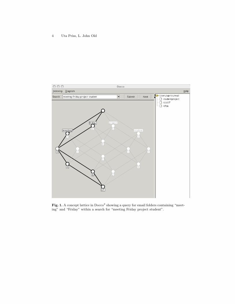
Fig. 1. A concept lattice in Docco2 showing a query for email folders containing “meet-ing” and “Friday” within a search for “meeting Friday project student”.


a lattice-based model which is in some ways similar to FCA. This lattice-basedinformation retrieval model was described by Mooers (1958) in a semi-formalmanner and elaborated with mathematical proofs by Woods (1964). Mooerscredits Fairthorne (1947, 1956) with being the first person to suggest using lat-tices for information retrieval. Mooers (1958) sees Boolean lattices as the mostimportant lattices. He describes different transformations from a space of “re-trieval prescriptions” into the lattice of all possible document subsets. Whilehis transformation T1 selects the set of documents that contain “exactly” therequested prescriptions, T2 selects the documents which contain “at least” therequested prescriptions. The transformation T2 represents “the well-known factthat as one adds more and more descriptors to a retrieval prescription, the set ofretrieved documents becomes smaller and smaller, and that each of the smallersets of documents is included within the larger set which is obtained with fewerdescriptors in a prescription” (Mooers, 1958, p. 1342). Thus, T2 is a Galois con-nection between documents and prescriptions. In FCA terms, Mooers’ discoverycould be described much simpler by stating that prescriptions are the formalobjects and the documents the formal attributes of a formal context (similar tothe example in Fig. 1, although upside down).

In general, the information retrieval problem is described by Mooers as aproblem of mappings between the space of retrieval prescriptions and the spaceof document descriptors. The mappings become more complicated if an addi-tional hierarchy is defined on the descriptors (such as a library classificationscheme), or if they can be combined using AND, OR and NOT. Woods (1964)and Soergel (1967) formalise and elaborate these mappings further. Woods’s pa-per was written as a student paper and would probably have been forgotten ifSalton had not included it in his book. Salton (1968) considers “inclusive retrievalfunctions” which are order-inverting maps between the retrieval space and thedocument space (because more prescriptions retrieve fewer documents and viceversa). The use of additional operators or of a classification system yields latticeswhich are even larger and more complicated than Boolean lattices. Salton showsa free distributive lattice resulting from three descriptors and a single operator,which has the meaning “having a topic in common” (p. 216). He also discussesthe problems of negation in some detail (p. 223-227).

One of Salton’s examples (p. 219) is shown in Fig. 2 (although with a slightlymore FCA-like notation). This example is very similar to concept lattices in FCA.The request space is a Boolean lattice of three prescriptions. But the space ofretrieved documents is not Boolean. In FCA terms, it is the concept lattice ofa formal context of prescriptions and documents. The dashed arrows show the(order-inverting) retrieval mapping from each document to its set of prescrip-tions. Unfortunately, neither Salton, nor Woods, Mooers or Soergel saw the po-tential of these kinds of non-Boolean lattices. Salton’s main interest was Booleanlattices because his concluding theorem shows under which circumstances theresulting lattice (as in Fig. 2) is Boolean.

As far as we know, Salton and Soergel eventually lost interest in lattices.Woods remains fascinated by lattices, but is less focused on their mathemat-


A

A,B,C

A,C B,CA,B

32

C B

A

1

4

Request space: prescriptions A, B, C

Space of retrieved documentsdocuments 1, 2, 3, 4

each document ismapped onto set ofprescriptions

B C

Fig. 2. Salton’s example - similar to a concept lattice, but 15 years before FCA!

ical details. Towards developing intelligent computer assistants, Woods (1978)proposes situation lattices. These organise “things to be done and goals to beachieved” into a conceptual taxonomy of situations (p. 33). A situation descrip-tion must be composite and structured, subparts of which will be instances ofother concepts, and makes use of concepts of objects, (substances, times, events,places, individuals) represented as configurations of attributes standing in spec-ified relationships to each other.

Woods credits Brachman (1978) for the generalisation, in his model, of thevarious notions of feature etc. to a single notion. “A concept node in Brachman’sformulation consists of a set of “dattrs” [parts, constituents, features etc.] ... someof which are represented directly at a node, and others are inherited from othernodes” (p. 34). Situation descriptions may subsume other situation descriptionsat lower levels of detail. “The space of possible situation descriptions forms alattice under subsumption. At the top of the lattice is a single, most generalsituation we will call T ... anything that is universally true can be stored here”(p. 38). Conversely at the bottom of the lattice is a situation that is neversatisfied.

A situation description can be made more general by (amongst other things)relaxing the constraints of a dattr, or made more specific by (amongst otherthings) tightening the condition on a dattr. Wood’s description of the situationlattice, because it is meant to be a model of the working memory of an intelligentmachine, is embedded in a complex description of situation recognition andclassification, spreading activation (Quillian, 1967) and marker propagation, andother functions incorporated to make the lattice dynamic. Thus, Woods sees the


potential of lattices for describing conceptual structures, but he does not providea precise mathematical description of how to implement these.

3 Lattices and Thesauri in Mechanical Translation

The second example of lattice-based modelling is in the field of what is nowadayscalled “natural language processing”. As mentioned in the introduction, Master-man et al. (1959) argue that there is a connection between both fields becausethey both belong to the field of “semantic transformation”. In 1956 at the Inter-national Conference on Mechanical Translation at MIT, four researchers fromthe Cambridge Language Research Group (Masterman (1956), Richens (1956),Parker-Rhodes (1956), Halliday (1956)) reported on their research of using athesaurus as an interlingua in “mechanical translation” (MT), the term thenused for “machine translation”. The group’s founder, Masterman, envisionedusing mathematical lattice theory for building a thesaurus, i.e. a hierarchicalstructure with grouping of synonyms or near synonyms. She thought that a“multilingual MT dictionary is analogous in various respects, to a thesaurus”and that “the entries form, not trees, but algebraic lattices, with translationpoints at the meets of the sublattices” (Masterman, 1956). The advantage ofthis approach is that instead of having to consider different pairs of languagesseparately, each language needs to be translated only once (into the thesaurus).Adding a new language does not require any changes to the previously addedlanguages. Masterman stated that “the complexity of the entries need not in-crease greatly with the number of languages, since translation points can, anddo, fall on one another.”

Of course, computational research in the 50s and 60s was influenced bythe limitations of computers at that time. Considerations about computationalspeed and storage problems determined the algorithms. Parker-Rhodes (1956)extended Masterman’s ideas by describing a mechanical translation program forsuch an interlingual thesaurus that uses Boolean operations which “can be per-formed with very great speed.” The storage problem would be solved by storing“all the relevant information ... in the input and output dictionaries”. Richens(1956) described the algebraic interlingua, NUDE, its code and an overview ofits translation operations.

MT algorithms in that time often started with a chunk-by-chunk literal trans-lation (Masterman et al, 1959). Every word stem and every grammatical indi-cator was translated from the input language to the output language using adictionary and some rules. Masterman’s use of lattices was novel because otherlinguists in that time (for example Lehmann (1978)) saw translation as a map-ping between trees. A sentence from the input language was parsed into a treestructure. Each branch of the input language was mapped onto a branch ofthe output language. The branches in the output language formed another treewhich had the output sentence as their root. Masterman argued that from asemantic viewpoint, lattices are a better model than trees. In a lattice, pairs ofelements can have different numbers of parents and children, instead of having


only one parent each in a tree structure. Thus combinations of meanings can berepresented more naturally.

In particular, Masterman (1957) was interested in Roget’s Thesaurus (RT).Her idea was that each of the 1000 categories in RT could be used as a “head”which described the core meaning of a word. Because a word can occur morethan once in RT, a word can have several heads. This leads naturally to a lattice,not tree structure. Of course, this implies that the meets and joins need tobe calculated; without meets and joins, a thesaurus would be just a partiallyordered set, not a lattice. Multiple occurrences of a word in the thesaurus mightcorrespond to different meanings of the word or even homographs (such as “lead”the verb and “lead” the material). If one determines the heads of all the wordsof a sentence, the heads can provide an indication of what the sentence is about.Individual words can be disambiguated by comparing their heads to the otherheads in the sentence. If a word has two different heads and only one of thesealso occurs for other words in the same sentence, then it is quite likely that thathead corresponds to the meaning of the word in this sentence.

Masterman et al. (1959) saw a relationship between MT and informationretrieval because in both cases a thesaurus could be used: either for retrievalor as an interlingua. Even syntax was dealt with by the thesaurus (Masterman,1957) because grammatical indicators in the “intralinguistic context” relate tostructures in the “extralinguistic context” that are shared across languages. Forexample, some languages have no genders (English), others have two (French),three (German) or six (Icelandic). But the distinction between “male” and “fe-male” is extralinguistically motivated. Masterman et al, (1959) see an interlin-gua as consisting of a “logical system giving the structural principle on which alllanguages are based”. In modern terminology, the thesaurus represents the “con-ceptual structures” that underly information retrieval and natural languages. Inour opinion, this is quite similar to Woods’ (1978) situation lattices. Becausedifferent languages share conceptual structures, they could share a thesaurus orconceptual structure. Only the lists of synonyms that were attached to every the-saurus head would be different in the different languages. Masterman was awareof Mooers’ use of lattices and saw this as further evidence for the connectionbetween the two fields.

4 Modern Descendants

The Mooers-Salton lattice-based retrieval model appears to have mostly beenforgotten until it was rediscovered in the context of FCA (cf. Priss (2000) for anoverview). Without being aware of the model in Salton’s book, FCA researchersbuilt formal contexts of documents and terms and studied their concept lattices(starting with Godin et al. (1989)). There are many FCA applications in thisarea. Just to name one example: Credo3 provides an on-line interface for websearch engines.

3http://credo.fub.it/


Masterman’s research influenced many people, including Karen Sparck Joneswho is considered to be one of the pioneers in information retrieval and naturallanguage processing. Sparck Jones used Roget’s Thesaurus, but as far as weknow had not much interest in lattices. Similarly, Yarowsky (1992) described animplementation of the use of Roget’s for word-sense disambiguation which wasvery similar to Masterman’s ideas (although he does not cite her), but he usesstatistical methods instead of lattices.

In 1960s in the US, Sally Yeates Sedelow obtained funding to convert theAmerican edition of Roget’s (1962) into a machine readable format with thepurpose of aiding machine translation. The initial abstract models that she andher husband, Walter Sedelow, used did not rely on lattice theory (Dillon (1971),Bryan (1973), Bryan (1974), Talburt & Mooney (1989)). But Bryan’s modeldescribes a binary relation between words and senses, which is very similar to aformal context as used in FCA. Thus when the Sedelows met Rudolf Wille, thefounder of FCA, in the early 1990s, they were enthusiastic about the possibilitiesthat lattice theory had to offer for their research. Their paper about the concept“concept” (Sedelow & Sedelow, 1993) derives semantic neighbourhoods for wordsfrom the thesaurus which are then represented as “neighbourhood lattices”. Ourown research has used and elaborated this technique in a variety of papers (Priss& Old, 2004) and has recently led to the implementation of an on-line interface4,which allows users to interactively generate such lattices. Thus, one can arguethat this modern research is an implementation of Masterman’s ideas, althoughthe thesaurus research (of the Sedelow’s) was initially separated from latticeresearch and was only recombined through FCA.

Another modern instantiation of Masterman’s ideas is Helge Dyvik’s (2004)research, although, as far as we know, he was not directly influenced by or awareof either FCA or Masterman. Dyvik’s lattices are feature lattices in the senseof componential semantics. Dyvik’s Semantic Mirrors Method extracts semanticinformation from bilingual corpora. His assumption is that if the same sentenceis expressed in two different languages, then it should be possible to align wordsor phrases in one language with the corresponding words or phrases in the otherlanguage using statistical processes or semi-automated processes. Once the cor-pora are aligned the “translational images” of words in the other language arecomputed. This process can be repeated several times. Next, the translationalimages are algorithmically assigned to separate senses. The resulting structurescan be represented either graphically as lattices, or as a thesaurus (using aWordNet-style representation). Both structures can be generated interactivelythrough an on-line interface5. Priss & Old (2005) have shown that this procedureis similar to creating neighbourhood lattices in FCA, though Dyvik’s researchwas developed independently of FCA.

It could be argued that Dyvik’s Semantic Mirror’s method is a proof of con-cept for Masterman’s vision. Masterman’s (1956) statement that a “multilingualMT dictionary is analogous in various respects, to a thesaurus” and that “the en-

4http://www.roget.org5http://ling.uib.no/helge/mirrwebguide.html


tries form, not trees, but algebraic lattices, with translation points at the meetsof the sublattices” prescribes exactly what Dyvik has implemented. Of course,it would not have been possible to implement a system like Dyvik’s in the 1950sor 60s due to the limits of computers at that time. It seems to us, however, thatmaybe not all of Masterman’s ideas have fully been explored using modern tech-nology. For example, the “Twenty questions method of analysis” (Mastermanet al 1959) that was used for extracting extralinguistic (or “semantic”) informa-tion via an intralingual analysis appears to be similar to attribute explorationin FCA (Ganter & Wille, 1999). But this relationship has not yet been furtherinvestigated.

The modern descendants of Quillian (1967), Brachman (1978) and Woods(1978) are terminological or description logics, conceptual graphs and formalontologies as used in the context of the Semantic Web. It appears to be generallyaccepted that the class or type hierarchies in these formalisms form lattices. Butapart from the class or type hierarchies, these systems also contain a variety ofother formal structures that do not form lattices. Thus Masterman’s view of athesaurus-lattice as the driving component in conceptual structures (or semantictransformations) was only partly correct. Lattices are important components,but not the only structures used in such systems. The connections between FCAand these fields have been established and are well documented (e.g. Rudolph(2006)).

5 Conclusion

In the introduction we questioned whether modern research in this area is acontinuation or just a repetition of ideas that were suggested 40-50 years ago;whether this old research still inspires modern work; and whether improvementsin hardware and software have made the old research obsolete. Returning tothese questions, it can be stated that the 1950s and 60s research about lattice-based modelling of thesauri was visionary, but hindered by the limitations ofthe computer hardware and software of that time. In both fields, natural lan-guage processing and information retrieval, the theoretical relevance of latticetheory has been acknowledged since the 50s and 60s. But non-FCA researcherstend to use non-lattice operations for most of their algorithms. Only the FCAresearchers in these fields focus on exploiting the lattice operations. Practicalimplementations of software using lattice theory have only been feasible sincethe 1990s. Some of these modern implementations (such as neighbourhood lat-tices of Roget’s Thesaurus or Dyvik’s Semantic Mirrors method) can be seenas “proof of concept” for ideas suggested in the 50s. But in modern research,thesauri and lattices are usually complemented with other structures under thegeneral heading of “conceptual structures”. Thus the older ideas have been val-idated and but also been extended in modern research. It ultimately remains tobe seen what role lattices play with respect to the conceptual structures that un-derly these disciplines, whether lattices are a core, driving force in such systems


or whether they are merely one formal model amongst many other contributingmodels.

References

1. Brachman, R. J. (1978). A Structural Paradigm for Representing Knowledge.Technical Report No. 3605, Bolt, Beranek and Newman Inc., Cambridge,MA. (Available from the US Defense Technical Information Center (DTIC),http://www.dtic.mil/ ).

2. Bryan, R. (1973). Abstract Thesauri and Graph Theory Applications to ThesaurusResearch. In: Sedelow, Sally Y. (ed.). Automated Language Analysis. Report onresearch 1972-73, University of Kansas, Lawrence.

3. Bryan, R. (1974). Modeling in Thesaurus Research. In: Sedelow, Sally Y. (ed.).Automated Language Analysis. Report on research 1973-74, University of Kansas,Lawrence.

4. Dillon, M.; Wagner, D. J. (1971). Models of thesauri and their applications. In:Sedelow, Sally Y. (ed.). Automated Analysis of Language Style and Structure inTechnical and other Documents. Technical Report, University of Kansas, Lawrence.

5. Dyvik, H. (2004). Translations as semantic mirrors: from parallel corpus to word-net. Language and Computers, 49, 1, Rodopi, p. 311-326.

6. Fairthorne, R. A. (1947). The Mathematics of Classification. Proc. British Societyof International Bibliography, 9, 4.

7. Fairthorne, R. A. (1956). The Patterns of Retrieval. American Documentation, 7,p. 65-75.

8. Ganter, B.; Wille, R. (1999). Formal Concept Analysis. Mathematical Foundations.Berlin-Heidelberg-New York: Springer.

9. Godin, R.; Gecsei, J.; Pichet, C. (1989). Design of browsing interface for informa-tion retrieval. In: N. J. Belkin, & C. J. van Rijsbergen (Eds.), Proc. SIGIR ’89, p.32-39.

10. Halliday, M. A. K. (1956). The Linguistic Basis of a Mechanical Thesaurus. Me-chanical Translation 3, 3, p. 81-88.

11. Lehmann, W. P.; Pflueger, S. M.; Hewitt, H.-J. J.; Amsler, R. A.; Smith, H. R.(1978). Linguistic Documentation of Metal System. Final technical report, RomeAir Development Center, RADC-TR-78-100.

12. Masterman, M. (1956). Potentialities of a Mechanical Thesaurus. MIT Conferenceon Mechanical Translation, CLRU Typescript. [Abstract]. In: Report on research:Cambridge Language Research Unit. Mechanical Translation 3, 2, p. 36.

13. Masterman, M. (1957). The Thesaurus in Syntax and Semantics. MechanicalTranslation, 4, 1 and 2, p. 35-43.

14. Masterman, M.; Needham, R. M.; Sparck-Jones, K. (1959). The Analogy betweenMechanical Translation and Library Retrieval. In: Proceedings of the InternationalConference on Scientific Information (1958). National Academy of Sciences - Na-tional Research Council, Washington, D.C., 1959, Vol. 2, p. 917-935.

15. Mooers, C. N. (1958). A mathematical theory of language symbols in retrieval. In:Proc. Int. Conf. Scientific Information, Washington D.C.

16. Parker-Rhodes, A. F. (1956). Mechanical Translation Program Utilizing an Inter-lingual Thesaurus. [Abstract]. In: Report on research: Cambridge Language Re-search Unit. Mechanical Translation 3, 2, p. 36.


17. Priss, U. (2000). Lattice-based Information Retrieval. Knowledge Organization, 27,3, p. 132-142.

18. Priss, U.; Old, L. J. (2004). Modelling Lexical Databases with Formal ConceptAnalysis. Journal of Universal Computer Science, 10, 8, p. 967-984.

19. Priss, U.; Old, L. J. (2005). Conceptual Exploration of Semantic Mirrors. In:Ganter; Godin (eds.), Formal Concept Analysis: Third International Conference,ICFCA 2005, Springer Verlag, LNCS 3403, p. 21-32.

20. Quillian, M. R. (1967). Word Concepts: A Theory and Simulation of Some BasicSemantic Capabilities. Behavioural Science 12, 5, p. 410-430.

21. Richens, R. H. (1956). General Program for Mechanical Translation between anytwo Languages via an Algebraic Interlingua. [Abstract]. In: Report on research:Cambridge Language Research Unit. Mechanical Translation 3, 2, p.37.

22. Roget, P. M. 1962. Roget’s International Thesaurus. 3rd Edition Thomas Crowell,New York.

23. Rudolph, S. (2006). Relational Exploration - Combining Description Logics andFormal Concept Analysis for Knowledge Specification. PhD Dissertation, Univer-sitatsverlag Karlsruhe.

24. Salton, G. (1968). Automatic Information Organization and Retrieval. McGraw-Hill, New York.

25. Sedelow, S.; Sedelow, W. (1993). The Concept concept. Proceedings of the Fifth In-ternational Conference on Computing and Information, Sudbury, Ontario, Canada,p. 339-343.

26. Soergel, D. (1967). Mathematical Analysis of Documentation Systems. InformationStorage and Retrieval, 3, p. 129-173.

27. Sowa, J. (2006). Categorization in Cognitive Computer Science. in: H. Cohen &C. Lefebvre (eds.), Handbook of Categorization in Cognitive Science, Elsevier, p.141-163.

28. Talburt, J. R.; Mooney, D. M. (1989). The Decomposition of Roget’s InternationalThesaurus into Type-10 Semantically Strong Components. Proceedings. 1989 ACMSouth Regional Conference, Tulsa, Oklahoma, p. 78-83.

29. Woods, W. A., Jr (1964). Mathematical Theory of Retrieval Systems. HarvardUniversity. Applied Mathematics 221, Student Research Report.

30. Woods, W. A. (1978). Taxonomic Lattice Structures for Situation Recognition.In: Proceedings of the 1978 Workshop on Theoretical Issues in Natural LanguageProcessing, p. 33-41.

31. Yarowsky, D. (1992). Word-sense disambiguation using statistical models of Roget’scategories trained on large corpora. In: Proc. COLING92, Nantes, France.


Piecewise-Linear Approximation of NonlinearModels Based on Interval Numbers (INs)

Vassilis G. Kaburlasos and S. E. Papadakis

Technological Educational Institution of KavalaDepartment of Industrial Informatics

65404 Kavala, Greecevgkabs,[email protected]

Abstract. Linear models are ususally preferable due to their simplicity.However, nonlinear models often emerge in practice. A popular approachfor dealing with nonlinearities is using a piecewise-linear approximation.In such context, inspired from both Fuzzy Inference Systems (FISs) ofTSK type and Self-Organizing Maps (SOMs), this work introduces en-hancements based on Interval Numbers and, ultimately, on lattice theory.Advantages include a capacity to deal with granular inputs, introductionof tunable nonlinearities, representation of all-order statistics, and induc-tion of descriptive decision-making knowledge (rules) from the trainingdata. Preliminary computational experiments here demonstrate a goodcapacity for generalization; furthermore, only a few rules are induced.

Key words: Fuzzy inference systems (FIS), Genetic optimization, Gran-ular data, Interval number (IN), Lattice theory, Linear approximation,Rules, Self-organizing map (SOM), TSK model

1 Introduction

The need to employ a real function y : RN → RM , i.e. a model, arises frequentlyin practice. In particular, linear models y(x) = c0 + c1x1 + c2x2 + ...+ cNxN arepreferable due to simplicity. However, most often, the dependence of output yon the input variables x1, ..., xN is nonlinear.

A popular approach for dealing with nonlinearities is using a piecewise-linearapproximation. For instance, in the context of fuzzy logic, the TSK (Tagaki-Sugeno-Kang) fuzzy model [13], [14], [15], [16] is popular. The computation of aTSK model, in the first place, involves the computation of clusters.

A popular scheme for clustering is the self-organizing map (SOM) devisedfor visualization of nonlinear relations of multidimensional data [10]. Lately,granular extensions of SOM were proposed in classification applications [8], [11],where a data cluster was represented by a fuzzy interval number (FIN).

This work proposes simpler acronym IN (Interval Number) for a FIN. In thesequel, it explains that a IN is a mathematical object, which may be interpretedas a probability/possibility distribution, an interval, and/or a real number. Inconclusion, inspired from TSK modeling, this work proposes lattice computing


techniques for an advantageous, piecewise-linear approximation based on a IN-extension of SOM.

We remark that the term lattice computing, or LC for short, was coinedlately to denote an emerging Computational Intelligence paradigm based onlattice theory [3]. More accurately, LC is defined here as an evolving collectionof tools and methodologies that can process disparate types of data includinglogic values, numbers, sets, symbols, and graphs based on mathematical latticetheory with emphasis on clustering, classification, regression, pattern analysis,and knowledge representation applications.

This paper is organized as follows. Section 2 describes the mathematical back-ground. Section 3 outlines the proposed techniques. Section 4 presents prelimi-nary experimental results. Section 5 concludes by summarizing the contribution.The Appendix summarizes the WRLS algorithm for incremental learning.

2 Mathematical Background

Here we summarize useful mathematical notions and tools regarding IntervalNumbers (INs) [4], [6], [7], [8] using an improved mathematical notation [9].

2.1 The Vector Lattice (∆,≤) of Generalized Intervals

Assume the complete latice (R,≤) of real numbers with least and greatest elementsdenoted, respectively, by O = −∞ and I = +∞. A generalized interval is definedin the following.

Definition 1. A generalized interval is an element of lattice (R,≤∂)×(R,≤).

We remark that ≤∂ in Definition 1 denotes the dual (i.e. converse) of orderrelation ≤, i.e. ≤∂≡≥. Moreover, product lattice (R,≤∂)×(R,≤) ≡ (R×R,≥ × ≤)will be denoted by (∆,≤).

A generalized interval is denoted by [x, y], where x, y ∈ R. Apparently, thecorresponding meet and join in lattice (∆,≤) are given, respectively, by [a, b] ∧[c, d] = [a ∨ c, b ∧ d] and [a, b] ∨ [c, d] = [a ∧ c, b ∨ d], where a ∧ c (a ∨ c) denotesthe minimum (maximum) of real numbers a and c.

The set of positive (negative) generalized intervals [a, b], characterized bya ≤ b (a > b), is denoted by ∆+ (∆−). Apparently, lattice (∆+,≤) of positivegeneralized intervals is isomorphic1 to the lattice (τ(R),≤) of intervals (sets) in R,i.e. (τ(R),≤) ∼= (∆+,≤). We have augmented lattice (τ(R),≤) by a least (empty)interval, denoted by O = [+∞,−∞]. Note that a greatest interval I = [−∞,+∞]

1A map ψ : (P,≤) → (Q,≤) is called (order) isomorphism if and only if both“x ≤ y ⇔ ψ(x) ≤ ψ(y)” and “ψ is onto Q”. Two lattices (P,≤) and (Q,≤) arecalled isomorphic, symbolically (P,≤) ∼= (Q,≤), if and only if there is an isomorphismbetween them.

14 Vassilis G. Kaburlasos, S. E. Papadakis

already exists in τ(R). Hence, the complete lattice (τO(R) = τ(R) ∪ O,≤)emerges — For simplicity, we use symbols O and I to denote the least andgreatest element, respectively, in any complete lattice.

A (strictly) decreasing bijective, the latter means “one-to-one”, function θR :R → R implies an isomorphism (R,≤) ∼= (R,≥); i.e. x < y ⇔ θR(x) > θR(y),x, y ∈ R. Furthermore, a strictly increasing function vR : R → R is a positivevaluation2 in lattice (R,≤). Therefore, function v∆ : ∆ → R given by v∆([a, b]) =vR(θR(a)) + vR(b) is a positive valuation in lattice (∆,≤) [5]. It follows a metricfunction d∆ : R → R≥0 given by d∆([a, b], [c, d]) = v∆([a, b] ∨ [c, d])− v∆([a, b] ∧[c, d]) = [vR(θR(a ∧ c)) − vR(θR(a ∨ c))] + [vR(b ∨ d) − vR(b ∧ d)]. In particular,metric d∆ is valid in lattice (∆+ ∪ O,≤) ∼= (τO(R),≤).

Functions θR(.) and vR(.) can be selected in many different ways. For in-stance, choosing both θR(x) = −x and vR(.) such that vR(x) = −vR(−x) itfollows positive valuation v∆([a, b]) = vR(b) − vR(a); hence, it follows metricd∆([a, b], [c, d]) = [vR(a∨ c)− vR(a∧ c)]+ [vR(b∨d)− vR(b∧d)] [6]. In particular,for θR(x) = −x and vR(x) = x it follows metric d∆([a, b], [c, d]) = |a− c|+ |b−d|.In general, parametric functions θR(.) and vR(.) may imply tunable nonlinearities.

The space ∆ of generalized intervals is a real linear space [4], [8] with

– addition defined as [a, b] + [c, d] = [a + c, b + d].– multiplication (by a scalar k ∈ R) defined as k[a, b] = [ka, kb].

A generalized interval in real linear space ∆ is also called vector. A lattice-ordered vector space is called vector lattice [4].

A subset C of a linear space is called cone if and only if for x1, x2 ∈ C andreal numbers λ1, λ2 ≥ 0 it follows (λ1x1 + λ2x2) ∈ C. It turns out that set ∆+

is a cone. Likewise, set ∆− is a cone.

2.2 The Cone Lattice (F,≤) of Interval Numbers (INs)

Generalized interval analysis in the previous section is useful for studying intervalnumbers (INs) in this section. A more general number type is defined first, inthe following.

Definition 2. A generalized interval number, or GIN for short, is a functionG : (0, 1] → ∆.

Let G denote the set of GINs. It turns out that (G,≤) is a complete latticesince (G,≤) is the Cartesian product of complete lattices (∆,≤).

Addition and multiplication are extended from ∆ to G as follows.

– The sum G1 + G2, G1, G2 ∈ G is defined as Gs : Gs(h) = (G1 + G2)(h) =G1(h) + G2(h), h ∈ (0, 1].

2Positive valuation is a function v : (L,≤) × (L,≤) → R, which satisfies bothv(x) + v(y) = v(x ∧ y) + v(x ∨ y) and x < y ⇒ v(x) < v(y).

Piecewise-Linear Approximation of Nonlinear Models Based on IntervalNumbers (INs)

15

– The product kG1, k ∈ R and G1 ∈ G, is defined as Gp : Gp(h) = kG1(h),h ∈ (0, 1].

Our interest here focuses on the sublattice3 of interval numbers defined next.

Definition 3. An Interval Number, or IN for short, is a GIN F such that bothF (h) ∈ (∆+ ∪ O) and h1 ≤ h2 ⇒ F (h1) ≥ F (h2).

Let F denote the set of INs. Conventionally, a IN will be denoted by a capitalletter in italics, e.g. F ∈ F. Moreover, a N -tuple IN will be denoted by a capitalletter in bold, e.g. F = (F1, ..., FN ) ∈ FN .

From Definition 3 it follows that a general IN F is written as the set unionof (conventional) intervals, e.g. F = ∪

h∈(0,1][ah, bh], where both interval-ends

ah and bh are functions of h ∈ (0, 1] such that ah ≤ bh.We point out that a IN is a mathematical object, which may be interpreted

as a probability/possibility distribution, an interval, and/or a real number. Forinstance, IN F = ∪

h∈(0,1][a, b] represents interval [a, b] including real numbers

for a = b. Moreover, a IN F may represent a probability distribution such thatinterval F (h) includes 100(1 − h)% of the distribution, whereas the remaining100h% is split even both below and above interval F (h) [4], [7], [8]. In addition,a IN may represent a fuzzy number as explained in subsection 2.3 below. In allcases, a IN can be interpreted as a granule (of information).

It has been shown that for F,E ∈ F there follow both (F ∧ E) ∈ F and(F ∨ E) ∈ F [9]. Hence, (F,≤) is a lattice with ordering F1 ≤ F2 ⇔ F1(h) ≤F2(h),∀h ∈ (0, 1].

The following proposition introduces a metric in lattice (F,≤) based on apositive valuation function vR : R → R≥0 [9].

Proposition 1. Let F1 and F2 be INs in the lattice (F,≤) of INs. Assumingthat the following integral exists, a metric function dF : F× F → R≥0 is given by

dF(F1, F2) =

1∫0

d∆(F1(h), F2(h))dh (1)

We remark that a Minkowski metric dp : FN × FN → R≥0 can be definedbetween two N -tuple INs F1 = [F1,1, ..., F1,N ]T and F2 = [F2,1, ..., F2,N ]T as

dp(F1,F2) = [dpF(F1,1, F2,1) + ... + dp

F(F1,N , F2,N )]1/p (2)

Minkowski metric dp(F1,F2) may involve a point x = [x1, ..., xN ]T ∈ RN suchthat an entry xi is represented by trivial IN xi = ∪

h∈(0,1][xi, xi], i = 1, ..., N .

Space F is a cone for F1, F2 ∈ F and real numbers λ1, λ2 ≥ 0 it follows(λ1F1 + λ2F2) ∈ F.

3A sublattice of a lattice (L,≤) is another lattice (S,≤) such that S ⊆ L.


2.3 Perspectives

A fundamental result in fuzzy set theory is the “resolution identity theorem”,which states that a fuzzy set can, equivalently, be represented either by its mem-bership function or by its α-cuts [19]. The aforementioned theorem was givenlittle attention in practice, to-date. However, some authors have capitalized onit by designing fuzzy inference systems (FIS) based on α-cuts of fuzzy numbers,i.e. based on intervals in τ(R) [17], [18]. More specifically, advantages includefaster (parallel) data processing “level-by-level” as well as “orders-of-magnitude”smaller computer memory requirements for representing, equivalently, fuzzy setswith arbitrary membership functions.

This work builds on the resolution identity theorem by, first, dropping thepossibilistic interpretation for a (fuzzy) membership function and, second, byconsidering its equivalent α-cuts (interval) representation.

3 The Proposed Techniques

This section outlines computational techniques for achieving a piecewise-linearapproximation of nonlinear models based on INs. Further details will be pre-sented in a future publication.

3.1 Structure Identification

Structure identification is a term from “fuzzy TSK system modeling” [12],[15],[16]meaning a partition of a model’s input space in subspaces, or clusters, such thatthe output to an “input point x = [x1, ..., xN ]T , within a cluster” is a (usu-ally) linear combination of the N inputs x1, ..., xN . It turns out that the task ofstructure identification is not trivial as illustrated in the following.

Consider the data points shown together with piecewise-linear approxima-tions of two different single-input-single-output models in Fig. 1(a) and Fig. 1(b),respectively. Fig. 1(a) demonstrates an effective partition (of the input space)characterized by a small approximation error, whereas Fig. 1(b) demonstratesan ineffective partition characterized by a large approximation error.

A structure identification method is proposed next based (1) on a novel SOMextension, and (2) on an advantageous, novel structure identification algorithm.

3.2 A SOM Extension

Each cell Ci,j in the SOM proposed here stores both a N -dimensional IN Fi,j =[Fi,j,1, ..., Fi,j,N ]T and a (N+1)-dimensional vector ci,j = [ci,j,0, ci,j,1, ..., ci,j,N ]T ,where i = 1, ..., I, and j = 1, ..., J . On one hand, IN Fi,j ∈ FN represents apopulation of data assigned to cell Ci,j . On the other hand, vector ci,j ∈ RN+1

stores the parameters of the following hyperplane

pi,j(x) = ci,j,0 + ci,j,1x1 + ci,j,2x2 + ... + ci,j,NxN (3)


17

Fig. 1. Two different, piecewise-linear single-input-single-output models. (a) Thismodel partitions the input space effectively with a small approximation error usingthree lines. (b) This model partitions the input space ineffectively with a large approx-imation error using two lines.

A cell is called nonempty if at least one datum is assigned to it. A nonemptycell represents a rule. In particular, the N INs in Fi,j of cell Ci,j correspondto a (fuzzy) rule antecedent, whereas the N + 1 hyperplane parameters in ci,j

constitute the corresponding rule’s consequent.

3.3 INSOM: A Structure Identification Algorithm

Structure identification is carried out using the novel algorithm INSOM, below.

3.4 Parameter Identification

Algorithm INSOM above induces an “initial” (piecewise-linear) model from aseries (xk, yk) ∈ RN × R, k = 1, 2, ..., n of training data. The objective in thissection is to compute a globally optimum model.

The output of the aforementioned “initial” model is written analytically as

y(xk) = c0 +L∑

i=1

(ci,0σi +N∑

j=1

ci,jσixk,j) (4)

where xk = [xk,1, ..., xk,N ]T , furthermore the σis are functions of the (known)INs. In conclusion, a globally optimum set of hyperplanes is computed by algo-rithm WRLS in the Appendix.

Further improvement was sought by optimal parameter estimation tech-niques, which replaced a IN Fi,j by IN F ′

i,j = ai,jFi,j + bi,j , where ai,j ∈ (0, 3] isa scaling parameter and bi,j ∈ [−1, 1] is a translation parameter, i = 1, ..., L, j =1, ..., N . More specifically, the task was to compute optimal INs F ′

i,j , in a meansquare error sense, by optimal parameter ai,j , bi,j estimation.

Optimization was pursued by genetic algorithms (GA) [1],[12], where thephenotype of an “individual” consisted of specific values of parameters ai,j , bi,j .There was a total number of 2×N ×L parameters binary-encoded to the chro-mosome of an “individual”. We included 25 “individuals” per generation.

In conclusion, we point out that our “initial” model was computed by al-gorithm INSOM for structure identification without any employment of fuzzy


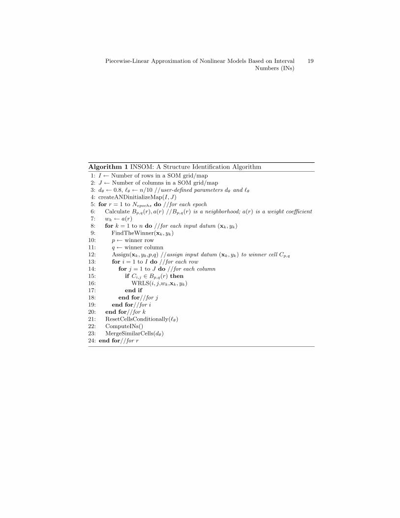
Algorithm 1 INSOM: A Structure Identification Algorithm1: I ← Number of rows in a SOM grid/map2: J ← Number of columns in a SOM grid/map3: dθ ← 0.8, `θ ← n/10 //user-defined parameters dθ and `θ4: createANDinitializeMap(I, J)5: for r = 1 to Nepochs do //for each epoch6: Calculate Bp,q(r), a(r) //Bp,q(r) is a neighborhood; a(r) is a weight coefficient7: wk ← a(r)8: for k = 1 to n do //for each input datum (xk, yk)9: FindTheWinner(xk, yk)

10: p← winner row11: q ← winner column12: Assign(xk, yk,p,q) //assign input datum (xk, yk) to winner cell Cp,q

13: for i = 1 to I do //for each row14: for j = 1 to J do //for each column15: if Ci,j ∈ Bp,q(r) then16: WRLS(i, j,wk,xk, yk)17: end if18: end for//for j19: end for//for i20: end for//for k21: ResetCellsConditionally(`θ)22: ComputeINs()23: MergeSimilarCells(dθ)24: end for//for r


19

logic. Whereas, thereafter, parameter identification was pursued based on stan-dard fuzzy TSK modeling techniques.

4 Preliminary Experimental Results

The effectiveness of our proposed (piecewise-linear approximation) techniques isdemonstrated in this preliminary work on a single-input-single-output nonlinearsystem. In the interest of simplicity positive valuation function vR(x) = x wasemployed. Furthermore, both input- and outputdata were normalized in theinterval [0, 1] by straightforward linear transformation. At the end of all com-putations, the output data were transformed back to their original domain formeaningful comparisons.

We considered the simple system described by the following equation.

y = sin(10x) (5)

where x ∈ [0, 1].Forty input/output data pairs (xk, yk) ∈ R × R, k = 1, ..., 40 were ran-

domly (uniformly) generated. The scatter plot of the generated input/outputdata points is shown in Fig. 2(a). Following a popular practice, we employed thesame data set for both training and testing. No validation set was employed.

A 4×4 SOM grid was used to compute a TSK model. The structure identifi-cation algorithm was applied for Nepochs = 100 epochs resulting in five nonemptycells — Recall that a nonempty cell represents a rule. The IN/antecedent andthe hyperplane/consequent (the latter is a line here) in each cell are shown inFig. 2(b) and Fig. 2(a), respectively. A visual inspection of Fig. 2 reveals thatthe proposed method partitions the input space well.

5 Conclusion

This work has proposed a new paradigm, inspired from both Fuzzy InferenceSystems (FISs) of TSK type and Self-Organizing Maps (SOMs), for piecewise-linear approximation of nonlinear models based on Interval Numbers (INs).

A unique advantage of INs here is their effectiveness in computing colinearpoints within a cluster as it will be detailed in a future publication. Another ad-vantage of our proposed techniques is the fast induction of an optimal number ofrules. Note that the employment of SOM in fuzzy system modeling applicationshas been rather sporadic to-date. Nevertheless, different authors have confirmedthe capacity of SOM for rapid data processing [2]. In our future work we havealso planned additional experiments including alternative data sets.


0,0 0,2 0,4 0,6 0,8 1,0

0,0

0,5

1,0

x

0,0 0,2 0,4 0,6 0,8 1,0

y=sin(x)

0,0

0,2

0,4

0,6

0,8

1,0

Fig. 2. (a) Scatter plot of function y = sin(10x) including 40 input/output data points.The five lines correspond, respectively, to the consequents of five rules. (b) The five INscorrespond, respectively, to the antecedents of five rules — Note that the correspondingconsequent (line) for a IN is shown above the IN.

Appendix

Here we show the Weighted Recursive Least Squares (WRLS) algorithm forincremental learning.

Consider a series of data vectors [xk,1, ..., xk,M , yk]T ∈ RM × R, k = 1, ..., n.The WRLS algorithm computes incrementally the parameters of a hyperplanein RM+1, optimally fitted, in a least square error sense, to the aforementioneddata. The corresponding equations are shown next.

ck+1 = ck +(yk+1 − xT

k+1 · ck

)kk

kk = Skxk+11

wk+xT

k+1Skxk+1

Sk+1 =(I− kkxT

k+1

)Sk

k = 1, 2, ..., n.

(6)

The equations above are initialized at k = 0 with c0 = 0 and S0 = aI, wherea ∈ R is typically large, e.g. a = 1000. Vector ck = [ck,0, ck,1, ..., ck,M ]T includesthe optimum hyperplane parameters at a step.

References

1. Cordon, O., Gomide, F., Herrera, F., Hoffmann, F., Magdalena, L.: Ten years ofgenetic fuzzy systems: current framework and new trends. Fuzzy Sets and Systems141(1) (2004) 5–31


21

2. Er, M. J., Li, Z., Cai, H., Chen, Q.: Adaptive noise cancellation using enhanceddynamic fuzzy neural networks. IEEE Trans. Fuzzy Systems 13(3) (2005) 331–342

3. Grana, M.: Lattice computing: lattice theory based computational intelligence. In:T. Matsuhisa, H. Koibuchi (eds) Proc. Kosen Workshop on Mathematics, Tech-nology, and Education (MTE), Irabaki National College of Technology, Ibaraki,Japan, 15-18 February 2008, pp. 19–27

4. Kaburlasos, V. G.: Towards a Unified Modeling and Knowledge-RepresentationBased on Lattice Theory. Springer, Heidelberg, Germany, ser Studies in Compu-tational Intelligence 27 (2006)

5. Kaburlasos, V. G., Athanasiadis, I. N., Mitkas, P. A.: Fuzzy lattice reasoning (FLR)classifier and its application for ambient ozone estimation. Intl. J. ApproximateReasoning 45(1) (2007) 152–188

6. Kaburlasos, V. G., Kehagias, A.: Novel fuzzy inference system (FIS) analysis anddesign based on lattice theory. part I: working principles. Intl. J. General Systems35(1) (2006) 45–67

7. Kaburlasos, V. G., Kehagias, A.: Novel fuzzy inference system (FIS) analysis anddesign based on lattice theory. IEEE Trans. Fuzzy Systems 15(2) (2007) 243–260

8. Kaburlasos, V. G., Papadakis, S. E.: Granular self-organizing map (grSOM) forstructure identification. Neural Networks 19(5) (2006) 623–643

9. Kaburlasos, V. G., Papadakis, S. E.: A granular extension of the fuzzy-ARTMAP(FAM) neural classifier based on fuzzy lattice reasoning (FLR). Neurocomputing(accepted).

10. Kohonen, T.: Self-Organizing Maps. Springer, Heidelberg, Germany, ser Informa-tion Sciences 30 (1995)

11. Papadakis, S. E., Kaburlasos, V. G.: Mass-grSOM: a flexible rule extraction forclassification. In: Proc. 5th Workshop Self-Organizing Maps (WSOM 2005), Paris,France, 5-8 September 2005, pp. 553–560

12. Papadakis, S. E., Theocharis, J. B.: A GA-based fuzzy modeling approach forgenerating TSK models. Fuzzy Sets and Systems 131(2) (2002) 121–152

13. Sugeno, M., Kang, G. T.: Fuzzy modelling and control of multilayer incinerator.Fuzzy Sets Systems 18(3) (1986) 329–346

14. Sugeno, M., Tanaka, K.: Successive identification of a fuzzy model and its ap-plications to prediction of a complex system. Fuzzy Sets Systems 42(3) (1991)315–334

15. Sugeno, M., Yasukawa, T.: A fuzzy-logic-based approach to qualitative modeling.IEEE Trans. Fuzzy Systems 1(1) (1993) 7–31

16. Takagi, T., Sugeno, M.: Fuzzy identification of systems and its applications tomodeling and control. IEEE Trans. Systems, Man & Cybernetics 15(1) (1985)116–132

17. Uehara, K., Fujise, M.: Fuzzy inference based on families of α-level sets. IEEETrans. Fuzzy Systems 1(2) (1993) 111–124

18. Uehara, K., Hirota, K.: Parallel and multistage fuzzy inference based on familiesof α-level sets. Information Sciences 106(1-2) (1998) 159–195

19. Zadeh, L. A.: The concept of a linguistic variable and its application to approximatereasoning - III. Information Sciences 9(1) (1975) 43–80


Computation of a Sufficient Condition forSystem Input Redundancy

S. E. Papadakis and V. G. Kaburlasos

Technological Institute of KavalaDepartment of Industrial Informatics

65404 Kavala, Greecespap,[email protected]

Abstract. The calculation of an optimal subset of inputs from a setof candidate ones is known in the bibliography of system modeling asthe input (or feature) selection problem. In this work we introduce aremarkable attribute of the FLR classifier: it’s capacity to identify re-dundant system inputs, from a set of input/output data. The proposedapproach is applicable beyond RN on any lattice ordered data set LN ,which may include disparate types of data. Also, the proposed approachcan deal with populations of data instead of crisp data vectors. Finally,it is highlighted that proposed approach can be employed for designingmodels with simple structure and significant performance. The methodis successfully applied here on two well known real world classificationproblems, identifying redundant inputs and inducing FLR classifiers withsimple structure and favorable classification performance.

Key words: Fuzzy Interval Number (FIN), Fuzzy Lattice Reasoning(FLR), classification, lattice theory

1 Introduction

One of the most important issues in computational intelligence is the structureidentification of the model to be used for modeling effectively a physical system.According to established modeling methodology, physical systems are treatedas black boxes where the only knowledge we have about them emanates from afinite set of samples, which are organized as ordered pairs of input (excitations)output (response) data. The next step in modeling, given a sufficient set ofinput/output data, is the definition of proper model’s structure and a learningrule. Since samples are always finite, an effective modeling must produce modelswith sound generalization capacities. That is, models which have as close aspossible behavior to physical system, especially on data lying outside the initialset of samples.

The related bibliography on effective model’s definition including fuzzy mod-eling [1–5], neural networks [6–8] , self organizing maps [9], mathematical models[10–12], etc is vast. In general, structure’s identification problem can be hierar-chically divided into three principal sub-problems. The first one, namely input


selection problem, is the choice from a set of (intuitively selected) candidateinputs of those ones that are necessary and sufficient to describe the specifiedtarget. Second, is the formation of inner model structure (i.e. number of rules, orneurons, input space partition etc.) in the space of selected inputs. Third, is theprocess of parameter identification (training) by applying a convenient learningrule.

The importance of input selection problem has been widely recognized bymany researchers [13, 14, 4] . For instance, in [3, 4] the authors claim that usinga scale of importance varying from one to one hundred, the input selectionproblem is rated as one hundred, the inner model’s structure is rated as ten,while the task of parameters identification is rated as one.

A detailed review of several input selection approaches is referred to in [13,15]. Although the proposed method encounter all aforementioned three types ofstructure identification problems, the discussion in this work focuses mainly oninput selection issues.

The basic advantage of our methodology, presented below, is that it can beapplied on non-homogeneous input/output data including real numbers, popula-tions of data represented by probability/possibility distributions,etc. Disparatetypes of data can be represented by Fuzzy Interval Numbers (FINs) [16–18]. Theset of FINs is lattice ordered, where a metric can be defined by establishing aparametric positive valuation function [16]. Parametric positive valuation func-tions introduce several tunable non-linearities, which are adjusted by a stochasticnon linear optimization method toward maximization of performance.

The layout of this preliminary work is as follows: Section 2 presents themathematical background. Section 3 presents the proposed method. Section 4presents experimental results. Finally, section 5 concludes by summarizing thecontribution of this work.


In order to make the proposed approach clear, some notions are shown next. Ageneralized interval is denoted by [x, y], x, y ∈ R. Let (∆,≤) = (R,≤∂)×(R,≤)be the complete product lattice of generalized intervals. Note that the inverse ≥of any order relation ≤ is itself an order relation. The order ≥ is called the dualof ≤, symbolically ≤∂ , or ≤−1, or ≥.

The corresponding meet and join in lattice (∆,≤) are given by [a, b]∧[c, d] =[a∨c, b∧d] and [a, b]∨ [c, d] = [a∧c, b∨d]. Note that (∆,≤) = (∆−,≤)∪(∆+,≤)where (∆−,≤) , (∆+,≤) is the set of negative (a > b) and positive (a ≤ b)generalized intervals, respectively. Note that lattice (∆+,≤) is isomorphic tolattice (τ(R),≤) of intervals in set R, That is (τ(R),≤) ∼= (∆+,≤).

A strictly decreasing function θR : R → R implies an isomorphism (R,≤) ∼= (R,≥). Furthermore, a strictly increasing function νR : R → R is a positivevaluation function in lattice (R,≤). Hence, function ν∆ : ∆ → R, given byν∆([a, b]) = νR(θR(a)) + νR(b) is a positive valuation function in lattice (∆,≤)[19]. It follows a metric d∆ : ∆×∆ → R+

0 given by

24 S. E. Papadakis, V. G. Kaburlasos

d∆([a, b], [c, d]) = [νR(θR(a ∧ c))− νR(θR(a ∨ c))] + [νR(b ∨ d)− νR(b ∧ d)] (1)

A Generalized Interval Number is a function f(0, 1] → ∆ where ∆ denotesa complete product lattice (∆,≤) = (R,≤∂)× (R,≤) of generalized intervals.

2.1 Fuzzy Interval Numbers

Fuzzy Interval Numbers or FINs have been extensively described in [16], [17],[18]. Let L to be the Lattice of FINs. Then a N-tuple FIN F ∈ LN . A FIN Fcan be represented as the union set of generalized intervals F = ∪

h∈(0,1][ah, bh].

IF ah = bh∀h ∈ (0, 1] the FIN is called trivial FIN. Given a strictly increasingfunction: ν(.) and a strictly decreasing one: θ(.) an inclusion measure is definedas a function σL : L× L → [0, 1], given by:

σL(F,E) =

1∫0

N∑i=1

[νR,i(θR,i(ci,h)) + νR,i(di,h)]

N∑i=1

[νR,i(θR,i(ai,h ∧ ci,h)) + νR,i(bi,h ∨ di,h)]dh (2)

Note that F,E are N-tuple FINs. Functions ν : R → R+0 and θ : R → R can

be given by:

νR,i(x) = Ai

1+e−λi(x−mi)

θR,i(x) = 1− 2mi

(3)

where i = 1, 2, ..., N . N denotes the number of inputs. Ai, λi,mi ∈ R tunableparameters. The size of a FIN is defined as a function ZF : F× F → R+

0 , givenby:

ZF (F) =

1∫0

d∆(ah, bh)dh (4)

where d∆(ah, bh) is computed by Eq. (1)

3 The Proposed Method

The granular FLR is a set of labeled pairs (Ei, ci) or granules , each representedby a N -tuple FIN Ei and a label ci. Linguistically, a granule defines a rule of theform: IF datum Fj is included in granule Ei then the class of datum Fj is ci.Hence a set RB = Ei, ci of granules defines a rule base for the FLR classifier.

The FLR algorithm is divided in two parts:

Computation of a Sufficient Condition for System Input Redundancy 25

Algorithm 1 FLR for training1: Initialize RB = E`, c` | ` = 1, 2, ..., L of granules E`. c` ∈ C is the label of granule

E`.2: Do set all pairs in RB. Present the next input pair (Fi, ci), i=1,...,n. Compute the

degree of inclusion σF (Fi ≤ E`) of input granule Fi to all granules E`, ` = 1, ..., L.3: IF no pairs are set in RB then store input pair (Fi, ci) in RB, L = L + 1, goto 2.4: The winner among set pairs in RB is Ej , cj such that j = arg max

`∈1,...LσF (Fi ≤ E`).

5: The Assimilation Condition: Both 1.) The size Z(Fi ∨ Ej) of granule Fi ∨ Ej isless than a user defined threshold size Zcrit and 2.) ci = cj .

6: if the Assimilation Condition is not satisfied then reset the winner and goto 3.Else, replace the winner with granule Fi ∧Ej ; and goto 2.

Algorithm 2 Stochastic optimization of tunable FLR parameters1: Select a population of individuals and encode Zcrit, Ai, λi, mi where i = 1, 2, ..., N

into chromosome.2: For each individual apply algorithm 1 and calculate its Fitness given by Eq. (5),

(see Section 4).3: Apply genetic operators to produce next generation.4: if stopping criterion is not satisfied then goto 2.5: Store the trained FLR, consisting of a RB of labeled granules and fine tuned pa-

rameters Zcrit, Ai, λi, mi.

The results of algorithm 1 depend on both Zcrit and parameters Ai, λi,mi |i =1, ..., N according to Eq. (2), (3). The tunable parameters Zcrit and parametersAi, λi,mi are optimized such that the rate of success classification is maximized.

In the case where νR,i(x) = consti ∀ x, i | consti ∈ R, it follows by equations1, 2 that any calculated distances and similarity measures take constant valuesfor every data Fj ,Fk 6=j . Hence, there is no any discretization information andall data are equally distant (or equally similar) to each other. The classificationprocess has to be entirely based only on the attributes (if any) with respectivenon flat sigmoid positive valuation functions. In other words attributes whichhave constant sigmoid positive valuation functions in the range of their interest,provides no discretization information and may be omitted. The aforementionedreasoning is experimentaly verified next.

4 Experimental Results

It has to be stressed that here we use input/output data, which are real numbers.However, the method has been developed using FINs data representation, whichare members of a lattice. Hence, without loss of generality, a FIN represents herea real number.


4.1 Fisher’s IRIS Classification Benchmark

Fisher Iris benchmark data set, downloaded from the UCI machine learningrepository [20], is used to demonstrate the proposed feature selection tech-nique. It includes measurements regarding four crinum flower attributes includ-ing x1:sepal-length, x2:sepal-width, x3:petal-length, x4:petal-width. The crinumsare classified in three classes, namely versicolor (i.e. class 1), setosa (i.e. class2), and virginica (i.e. class 3). In all, there are fifty 4-dimensional vectors perclass available. After a random data permutation we employed the first 50 datavectors (33.33%) for training the next 50 (33.33%) for validation and the last50 (33.33%) for testing. Each input datum is considered as a 4-tuple trivialFIN. Each sigmoid νi(x) | i = 1, 2, 3, 4, is defined by three tunable parametersAi, λi,mi.

The genetic algorithm, presented in [21], is used for the optimization of FLR.The optimization of FLR lies in the calculation of sigmoid’s parameter such thatthe rate of successful classification on both training and validation data set is ashigh as possible. Sigmoid parameters are binary encoded into the chromosomeof every individual, using a word of 16 bits per parameter. Each individual rep-resents a FLR model which is created using the encoded parameters’ value, andapplying the algorithm 2 on the training data set. Hence, the percent classifi-cation rate on both training and validation data set, namely (Rtrn) and (Rval)respectively, is calculated. The fitness function is calculated by Eq. (5)

Q(ps) = w ·Rtrn + (1− w) ·Rval +0.1L

(5)

The parameter ps = [Zcrit, A1, λ1,m1, ..., AN , λN ,mN ] denotes the vector oftunable parameter values, which are encoded into the chromoshome of individuals, s = 1, 2, ...S | S denotes the population size. For N attributes the vector ps has3N + 1 elements. Parameter L is a positive integer, which depends on the valueof parameter Zcrit and denotes the number of granules in RB that constitute theFLR model. Term 0.1/L in Eq. (5) is used to lead the evolution into FLR modelswith RB having small number of granules. Finally, w = 0.5 is a relaxation factor,used to direct the evolution out of over trained solutions. The GA populationincludes 25 individuals and the evolution terminates when the quality functionof the elite individual remains intact for 50 successive generations.

The sigmoid functions of the trained FLR are illustrated in Fig. 1. Stated byexperimental results, we conclude that attribute sepal width is negligible, sinceall sepal width input values are mapped to a constant value approximately equalto 2. As a result attribute sepal width does not provides any class discretizationinformation and should be removed. Our claim was experimentally verified by re-calculating the classification rate without using sepal width values. We remarkedthat ignorance of sepal width does not affect training, validation and checkingclassification rate.


8,06,04,0

5,04,03,02,0

3,0

2,5

2,0

1,5

1,0

0,5

0,0

7,04,01,0

3,0

2,5

2,0

1,5

1,0

0,5

0,0

2,01,00,0

3,0

2,5

2,0

1,5

1,0

0,5

0,0

Sepal Length Petal Length

Sepal witdh Petal Witdh

v1(x) v3(x)

v2(x) v4(x)

3,0

2,5

2,0

1,5

1,0

0,5

0,0

Fig. 1. The sigmoid positive valuation functions of the four attributes for the Fisher’sIRIS classification benchmark.Since the sigmoid function for Sepal width is flat weconclude that the corresponding input is redundant.

4.2 The Wine Classification Benchmark

A more complex problem, the well known wine classification benchmark, is usedin this example for further verification of proposed approach. In this problemis faced the classification of wines, in three categories according to 13 measuredchemical attributes. Each input datum is created as a 13-tuple trivial FIN. Eachdatum’s output takes an integer value 1,2, or 3 which represents the class ofspecific wine sample. The total of 178 input - output data were separated in threesubsets, namely, training (60 data), validation (60 data) and testing (58 data) set.Algorithm FLR was applied using all 13 attributes. After training, the sigmoidfunctions of attributes are illustrated in Fig. 2. It is clearly observed that sixattributes: Alcohol, Alkalinity of Ash, Magnesium, Total phenols, Nonflavonoidphenols and Proanthocyanins illustrate flat sigmoid in the range of interest.Thus, they are redundant. Ignoring redundant attributes a simplified FLR modelclassifier was built, which provides the same classification rate with FLR createdby all thirteen attributes. This result confirms experimentally the statement thatspecific attributes are unnecessary.

5 Discussion and Conclusion

A novel and effective method for the determination of redundant attributes inclassification problems was introduced. Our proposed method for input selection


Malic acid

5,95,24,43,73,02,21,50,7

3,0

2,0

1,0

0,0

Alcohol

15,014,013,012,011,0

15,0

14,5

14,0

Ash

3,12,72,21,81,3

1,0

0,5

0,0

Alcalinity of ash

30,025,020,015,010,0

10,0

9,5

9,0

Magnesium

157,5140,0122,5105,087,570,0

110,0

105,0

100,0

Total phenols

4,03,02,01,0

1,0

0,5

0,0

Flavanoids

5,44,12,71,4

0,8

0,4

0,0

Nonflavanoid phenols

0,70,50,40,30,1

1,0

0,5

0,0

Proanthocyanins

3,63,22,82,42,01,61,20,80,4

2,0

1,0

0,0

Color intensity

12,010,08,06,04,02,0

3,0

2,0

1,0

Hue

1,51,00,5

1,0

0,5

0,0

OD280/OD315 of diluted wines

4,03,02,01,0

1,0

0,5

0,0

Proline

1500,01000,0500,0

150,0

100,0

50,0

0,0

v1(x) v2(x) v3(x)

v4(x) v5(x) v6(x)

v7(x) v8(x) v9(x)

v10(x) v11(x) v12(x)

v13(x)

Fig. 2. The wine Classification Benchmark. Attributes with flat sigmoid positive valua-tion functions are redundunt ones since all their input values are mapped to a constantnumber.


using the FLR classifier computes only sufficient conditions. Hence when thesigmoid (positive valuation function) is constant in the range of interest of aninput variable then we conclude that the latter input variable is redundant andcan be omitted. In other words, for not-constant positive valuation functionswe cannot tell whether the corresponding input variable is redundant or not.More work needs to be done in this direction in the future. Considering that weneed only three tunable parameters per classifier’s input, we conclude that theproposed methodology produces FLR classifiers with simple structure. Moreover,the proposed technique is applied on data sets which are Lattices. In a futurework our proposed method will be applied on disparate types of data as symbolsand populations of measurements represented by probability distributions.

References

1. Papadakis, S., Theocharis, J.: A GA-based fuzzy modeling approach for generatingTSK models. Fuzzy Sets and Systems 131 (2002) 121–152

2. Simpson, P.: Fuzzy min-max neural networks -part i: Classification. IEEE Trans-actions on Neural Networks 3 (1992) 776–786

3. Sugeno, M., Tanaka, K.: Successive identification of a fuzzy model and its ap-plications to prediction of a complex system. Fuzzy Sets and Systems 42 (1989)315–334

4. Sugeno, M., Yasukawa, T.: A fuzzy-logic-based approach to qualitative modeling.IEEE Trans. Fuzzy Syst. 1 (1993) 7–31

5. Wang, X., Baets, B., Kerre, E.: A comparative study of similarity measures. FuzzySets and Systems 73 (1995) 259–268

6. Chakraborty, D., Pal, N.: A neuro-fuzzy scheme for simultaneous feature selectionand fuzzy rule-based classification. IEEE Transactions on Neural Networks 15(2004) 110–123

7. Patra, J., Pal, R., Chatterji, B., Panda, G.: Identification of nonlinear dynamicsystems using functional link artificial neural networks. IEEE Transactions onSystems, Man, and Cybernetics, Part B 29 (1999) 254–262

8. Rost, B., Sander, C.: Prediction of protein secondary structure at better than 70%accuracy. Journal of Molecular Biology 232 (1993) 584–599

9. Kohonen, T., Somervuo, P.: How to make large self-organizing maps for nonvec-torial data. Neural Networks 15 (2002) 945–952

10. Lichstein, J., Simons, T., Shriner, S., Franzreb, K.: Spatial autocorrelation andautoregressive models in ecology. Ecological Monographs 72 (2002) 445–463

11. Rabiner, Lawrence, R., Juang, Biing-Hwang: Introduction to hidden markov mod-els. IEEE ASSP magazine 3 (1986) 4–16

12. Zhang, B.: An EM algorithm for a semiparametric finite mixture model. Journalof Statistical Computation and Simulation 72 (2002) 791–802

13. Arauzo-Azofra, A., Benitez, J., Castro, J.: Consistency measures for feature selec-tion. Journal of Intelligent Information Systems 30 (2008) 273–292

14. Ivakhnenko, A., Ivakhnenko, N.: Long-term prediction of random processes bygmdh algorithms using the unbiasedness criterion and balance-of-variables crite-rion. Soviet Automation and Control 7 (1974) 40–45

15. Papadakis, S., Tzionas, P., Kaburlasos, V., Theocharis, J.: A genetic based ap-proach to the Type I structure identification problem. Informatica 16 (2005)365–382


16. Kaburlasos, V.: FINs lattice theoretic tools for improving prediction of sugarproduction from population of measurements. IEEE Transactions on System Manand Cybernetics, Part-B 34 (2004) 1017–1030

17. Kaburlasos, V., Papadakis, S.: Granular self organizing map (grSOM) for structureidentification. Neural Networks 19 (2006) 623–643

18. Papadakis, S., Marinagi, C., Kaburlasos, V., Theodorides, M.: Estimation of indus-trial production using the granular self-organizing map (grSOM). In: Proceedingsof the 12th Mediterranean Conference on Control and Automation (MED’04), Ku-sadasi, Turkey (2004) session TuM2-D,proceedings in CD-ROM.

19. Kaburlasos, V., Athanasiadis, I., Mitkas, P.: Fuzzy lattice reasoning (FLR) clas-sifier and its application for ambient ozone estimation. International Journal ofApproximate Reasoning 45 (2007) 152–188

20. Newman, D., Hettich, S., Blake, C., Merz, C.: UCI repository of machine learningdatabases. (1998)

21. Kazarlis, S., Papadakis, S., Theocharis, J.B., Petridis, V.: Micro-genetic algorithmsas generalized hill-climbing operators for GA optimazation. IEEE Transactions onEvolutionary Computation 5 (2001) 204–217


An Approach from Lattice Computing to fMRI Analysis

Manuel Graña, Maite García-Sebastián, Ivan Villaverde, Elsa Fernandez

Grupo de Inteligencia Computacional, UPV/EHUwww.ehu.es/ccwitnco

Abstract. We introduce an approach to fMRI analysis based on the Lattice As-sociative Memory (LAM) Endmember Induction Heuristic Algorithm (EIHA).Induced endmembers are used to compute the activation levels of voxels as resultof an unmixing process. The endmembers correspond to diverse activation pat-terns, one of these activation patterns corresponds to the rest state of the neuronaltissue. We introduce a lattice normalization which consists in the mean centeringfor each voxel patttern independently. This lattice normalization is needed to re-move scaling effects that rendered our approach inapplicable. Results on a casestudy are encouraging.

1 Introduction

Human brain mapping is a rapidly expanding discipline, and in recent years interest hasgrown in novel methods for imaging human brain functionality. Noninvasive techniquescan measure cerebral physiologic responses during neural activation. One of the rele-vant techniques is functional magnetic resonance imaging (fMRI) [6], which uses theblood oxygenation level dependent (BOLD) contrast. Slight physiological alterations,such as neuronal activation resulting in changes of blood flow and blood oxygenation,are detected. These signal changes are related to changes in the concentration of deoxy-hemoglobin, which acts as an intravascular contrast agent for fMRI. The most fMRIexaminations are performed with BOLD-based methods using techniques sensitive tolocal distortions in the magnetic field (susceptibility sensitive techniques). These are T2weighted spin echo pulse sequences or T2* weighted gradient echo pulse sequences.The various fMRI-methods have a good spatial and temporal resolution, limited onlyby the precision with which the autoregulatory mechanisms of the brain adjust bloodflow in space to the metabolic demands of neuronal activity. Since these methods arecompletely noninvasive, using no contrast agent or ionizing radiation, repeated single-subject studies are becoming feasible [5].

To evaluate the resulting fMRI image series, sophisticated algorithms and greatcomputational power are needed to separate the physiologically induced signals fromnoise or from artifacts resulting from patient movement or MRI detection techniques[13]. Appropriate postprocessing procedures for fMRI are currently being developed ata very rapid pace. Since many research groups are working in this area, no consensushas been reached about the analysis methods of the functional data up to now. A fur-ther reason for the large variety of different postprocessing procedures is the lack of acomplete underlying theory of the BOLD effect.


The fMRI experiment consists of a functional template or protocol (e.g., alternat-ing activation and rest for a certain time) that induces a functional response in thebrain.The aim of an fMRI experiment is to detect this stimulus response, resulting fromthe BOLD effect, in a defined volume element (voxel). The functional information ofa voxel has to be extracted from its functional time course. Therefore, for each func-tional time point one fMRI volume is recorded. The complete four-dimensional dataset(three dimensions in space, one dimension in time) consists of subsequently recordedthree-dimensional (3-D) volumes and thus for each voxel of a volume a functional timecourse exists. The acquisition of these functional volumes runs over periods lasting upto several minutes.

There are a number of sources of noise in the fMRI signal [14] that must be dealtwith in appropriate preprocessing steps. The pulse sequence and the magnetic fieldstregth used can have an effect on the image quality. The long time duration of theexperiments allow for head motions, even with strong restriction put into place. Experi-ment designs also affect the relative dynamics. We will assume that these noise sourceshave been dealt with appropriately.

The most extended analysis approach for fMRI signals is the Statistical ParametricMaps (SPM) [2] which has developed into a free open source software package. Thismethod consists in the separate voxel based test of the generalized linear model (GLM)corresponding to the experimental design, followed by a segmentation of the spatialdistribution of the individual voxel t-test values as a parametric map. There have beenalso approximations based on the Independent Component Analysis (ICA) [1] assum-ing that the time series observations are linear mixtures of independent sources whichcan not be observed. ICA assumes that the source signals are non-Gaussian and thatthe linear mixing process is unknown. The approaches to solve the ICA process ob-tain both the independent sources and the linear unmixing matrix. In previous workswe have proposed an heuristic algorithm, which we have called Endmember InductionHeuristic Algorithm (EIHA) in [3] to solve a similar problem. There the assumption isthat the data is generated from a set of endmembers which are the vertices of a convexpolytope covering the data observations. Our approach is based on the relation betweenthe Lattice Independence and Affine Independence [12], and the ability of Lattice As-sociative Memories to serve as detectors of Lattice Independent sets of vectors. Theoriginal works were devoted to unsupervised hyperspectral image segmentation, andhere we try to apply it to fMRI analysis. The results are promising. This approach fallsin the field of Lattice Computing algorithms, which have been introduced in [4] as theclass of algorithms that either apply lattice operators inf and sup or use lattice theoryto produce generalizations or fusions of previous approaches. In [4] an extensive andupdated list of references, including previous works from authors contributing to thisworkshop, can be found.

The outline of the paper is as follows: Section 2 will present the undelying linearmixing model. Section 3 presents an sketch of the relation between Lattice Indepen-dence and Linear (Affine) Independence through the LAM theory. Section 4 recalls ourheuristic algorithm. Section 5 presents results of the proposed approach on a case study.Section 6 provides some conclusions.

34 Manuel Grana, Maite Garcıa-Sebastian, Ivan Villaverde, Elsa Fernandez

2 The Linear Mixing Model

The linear mixing model can be expressed as follows:

x =M∑i=1

aisi + w = Sa + w, (1)

where x is the d-dimension pattern vector corresponding to the fMRI voxel time seriesvector, S is the d×M matrix whose columns are the d-dimension vertices of the convexregion covering the data corresponding to the so called endmembers si, i = 1, ..,M, ais the M -dimension fractional abundance vector, and w is the d-dimension additive ob-servation noise vector. The linear mixing model is subjected to two constraints on theabundance coefficients. First, to be physically meaningful, all abundance coefficientsmust be non-negative ai ≥ 0, i = 1, ..,M. Second, to account for the entire composi-tion, they must be fully additive

∑Mi=1 ai = 1. That means that we expect the vectors

in S to be affinely independent and that the convex region defined by them includes allthe data points.

Once the convex region vertices have been determined the unmixing process is thecomputation of the matrix inversion that gives the coordinates of the point relative tothe convex region vertices. The simplest approach is the unconstrained least squarederror (LSE) estimation given by:

a =(ST S

)−1ST x. (2)

The coefficients that result from equation 2 do not necessarily fulfill the non-negativityand full additivity conditions. For simplicity, we will use the unconstrained estimationof equation 2 to compute the abundance coefficients. Moreover, the heuristic algorithmEIHA described in section 4 from [3] always produces convex regions that lie inside thedata cloud, so that enforcing the non-negative and additivity to one conditions would beimpossible for some data points. Negative values are considered as zero values and theadditivity to one condition is not important as long as we are looking for the maximumabundances to assign meaning to the resulting spatial distribution of the coefficients.These coefficients are interpreted as fMRI voxel activation. That is, high positive val-ues are interpreted as high voxel activation if the corresponding endmember does notcorrespond to the random pattern obtained as the resting state response.

3 Lattice Independence and Lattice Autoassociative Memories

The work on Lattice Associative Memories (LAM) stems from the consideration ofthe algebraic lattice structure (R,∨,∧,+) as the alternative to the algebraic frameworkgiven by the mathematical field (R,+, ·) for the definition of Neural Networks compu-tation. The LAM were first introduced in [8,9] as Morphological Associative Memories,but we follow the new convention introduced in [11,12] because it sets the works in themore general framework of Lattice Computing. The operators ∨ and ∧ denote, respec-tively, the discrete max and min operators (resp. sup and inf in a continuous setting).

An Approach from Lattice Computing to fMRI Analysis 35

Given a set of input/output pairs of pattern (X, Y ) =(

xξ,yξ); ξ = 1, .., k

, a linear

heteroassociative neural network based on the pattern’s cross correlation is built up asW =

∑ξ yξ ·

(xξ

)′. Mimicking this constructive procedure [8,9] propose the following

constructions of Lattice Memories (LM):

WXY =k∧

ξ=1

[yξ ×

(−xξ

)′]and MXY =

k∨ξ=1

[yξ ×

(−xξ

)′], (3)

where × is any of the ∨2 or ∧2 operators. Here ∨2 and ∧2 denote the max and minmatrix product [8,9]. respectively defined as follows:

C = A ∨2 B = [cij ] ⇔ cij =∨

k=1,...,n

aik + bkj , (4)

C = A ∧2 B = [cij ] ⇔ cij =∧

k=1,...,n

aik + bkj . (5)

If X = Y then the LM memories are Lattice Autoassociative Memories (LAM).Conditions of perfect recall by the LM and LAM of the stored patterns proved in [8,9]encouraged the research on them, because in the continuous case, the LAM is ableto store and recall any set of patterns: WXX ∨2 X = X = MXX ∧2 X, for any X .However, this result holds when we deal with noise-free patterns. Research on robustrecall [7,9,10] based on the so-called kernel patterns lead to the notion of morphologicalindependence, in the erosive and dilative sense, and finally to the definition of LatticeIndependence (LI) and Strong Lattice Independence (SLI). We gather some results from[12] that set the theoretical background for the approach to endmember induction ap-plied.

Definition 1. Given a set of vectorsx1, ...,xk

⊂ Rn a linear minimax combination

of vectors from this set is any vector x ∈Rn±∞ which is a linear minimax sum of these

vectors:

x = L(x1, ...,xk

)=

∨j∈J

k∧ξ=1

(aξj + xξ

),

where J is a finite set of indices and aξj ∈ R±∞ ∀j ∈ J and ∀ξ = 1, ..., k.

Definition 2. The linear minimax span of vectorsx1, ...,xk

= X ⊂ Rn is the set of

all linear minimax sums of subsets of X, denoted LMS(x1, ...,xk

).

Definition 3. Given a set of vectors X =x1, ...,xk

⊂ Rn, a vector x ∈Rn

±∞ islattice dependent if and only if x ∈ LMS

(x1, ...,xk

). The vector x is lattice inde-

pendent if and only if it is not lattice dependent on X. The set X is said to be latticeindependent if and only if ∀λ ∈ 1, ..., k , xλ is lattice independent of X\

xλ

=

xξ ∈ X : ξ 6= λ

.

The definition of lattice independence supersedes and improves the early defini-tions [10] of erosive and dilative morphological independence, which, however, havemore intuitive appealing. Nevertheless, this definition has the additional advantage ofestablishing a formal parallelism with the definition of linear independence.


Definition 4. A set of vectors X =x1, ...,xk

⊂ Rn is said to be max dominant if

and only if for every λ ∈ 1, ..., k there exists and index jλ ∈ 1, ..., n such that

xλjλ− xλ

i =k∨

ξ=1

(xξ

jλ− xξ

i

)∀i ∈ 1, ..., n .

Similarly, X is said to be min dominant if and only if for every λ ∈ 1, ..., k thereexists and index jλ ∈ 1, ..., n such that

xλjλ− xλ

i =k∧

ξ=1

(xξ

jλ− xξ

i

)∀i ∈ 1, ..., n .

The expressions that compound this definition appeared in the early theorems aboutperfect recall of Morphological Associative Memories [8,9]. Their value as an identi-fiable property of the data has been discovered in the context of the formalization ofthe relationship between strong lattice independence, defined below, and the classicalaffine independence.

Definition 5. A set of lattice independent vectorsx1, ...,xk

⊂ Rn is said to be

strongly lattice independent (SLI) if and only if X is max dominant or min dominant orboth.

As said before, min and max dominance are the conditions for perfect recall. Perconstruction, the column vectors of Lattice Autoassociative Memories are min or maxdominant, depending of their erosive or dilative nature, therefore they will be stronglylattice independent, if they are lattice independent.

Conjecture 1. [12] If X =x1, ...,xk

⊂ Rn is strongly lattice independent then X

is affinely independent.

This conjecture (stated as theorem in [11]) is the key result whose proof wouldrelate the linear convex analysis and the non-linear lattice analysis. If true, it meansthat the construction of the LAM provides the starting point for obtaining sets of affineindependent vectors that could be used as endmembers for the unmixing algorithmsdescribed in section 2.

Theorem 1. [12] Let X =x1, ...,xk

⊂ Rn and let W ( M ) be the set of vectors

consisting of the columns of the matrix WXX (MXX .). Let F (X) denote the set of fixedpoints of the LAM constructed from set X . There exist V ⊂ W and N ⊂ M such that Vand N are strongly lattice independent and F (X) = F (V ) = F (N) or, equivalently,WXX = WV V and MXX = MNN .

The key idea of this theorem is to test the lattice independence of the already knownas min or max dominant sets of vectors. Removing lattice dependent vectors will notaffect this min/max dominance property. The smart way to test lattice dependence lies inthe fact that removing a lattice dependent vectors does not alter the set of fixed points ofthe remaining ones. This theorem is proved following a constructive reasoning, givingway to an algorithm for the construction of the set of affine independent sets of vectorsfrom LAM dicussed in [3,12].


Algorithm 1 Endmember Induction Heuristic Algorithm (EIHA)1. Shift the data sample to zero meanf c (i) = f (i)−−→µ ; i = 1, .., n.

2. Initialize the set of vertices E = e1 with a randomly picked sample. Initialize the set oflattice independent binary signatures X = x1 =

˘`e1

k > 0; k = 1, .., d´¯

3. Construct the LAM’s based on the lattice independent binary signatures: MXX and WXX .4. For each pixel f c (i)

(a) compute the noise corrections sign vectorsf+ (i) = (f c (i) + α−→σ > 0) and f− (i) =(f c (i)− α−→σ > 0)

(b) compute y+ = MXX ∧2 f+ (i)(c) compute y− = WXX ∨2 f− (i)(d) if y+ /∈ X or y− /∈ X then f c (i) is a new vertex to be added to E, execute once 3 with

the new E and resume the exploration of the data sample.(e) if y+ ∈ X and f c (i) > ey+ the pixel spectral signature is more extreme than the stored

vertex, then substitute ey+ with f c (i) .(f) if y− ∈ X and f c (i) < ey− the new data point is more extreme than the stored vertex,

then substitute ey− with f c (i) .

5. The final set of endmembers is the set of original data vectors f (i) corresponding to the signvectors selected as members of E.

4 Endmember Induction Heuristic Algorithm (EIHA)

For the sake of completeness we recall here our Endmember Induction Heuristic Al-gorithm (EIHA) maintaining the notation used in the original references. Let us denotef (i) ∈ Rd; i = 1, .., n

the high dimensional data that may be the time series in a

fMRI voxels, −→µ and −→σ are, respectively, the mean vector and the vector of standarddeviations computed over the data sample, α the noise correction factor and E the setof already discovered vertices. The noise amplitude of the additive noise in equation(1) is −→σ , the patterns are corrected by the addition and subtraction of α−→σ, before be-ing presented to the LAM’s. The gain parameter α controls the amount of flexibility inthe discovering of new endmembers. Let us denote by the expression x > 0 the con-struction of the binary vector (bi = 1 if xi > 0; bi = 0 if xi ≤ 0 ; i = 1, .., n) . Thedetailed description of the steps in the heuristic algorithm is presented as Algorithm 1.The starting endmember set consists of a randomly picked pixel. However, this selectionis not definitive, because the algorithm may later change this endmember for another,more extreme, one. The noise correction parameter α has a great impact on the numberof endmembers found. Low values imply large number of endmembers. It determinesif a vector is interpreted as a random perturbation of an already selected endmember.

5 A Case Study

The experimental data corresponds to auditory stimulation test data of single person. Itis freely available from ftp://ftp.fil.ion.ucI.ac.uk/spm/data, the file name is snrfM00223.zip.These data are the result of the preprocessing pipeline that removes many noise sources.


These whole brain BOLD/EPI images were acquired on a modified 2T Siemens MAG-NETOM Vision system. Each acquisition consisted of 64 contiguous slices. Each slicebeing a 2D image of one head volume cut. There are 64x64x64 voxels of size 3mm x3mm x 3mm. The data acquisition took 6.05s, with the scan-to-scan repeat time (RT)set arbitrarily to 7s. 96 acquisitions were made (RT=7s) in blocks of 6, i.e., 16 42sblocks. The condition for successive blocks alternated between rest and auditory stim-ulation, starting with rest. Auditory stimulation was bi-syllabic words presented bin-aurally at a rate of 60 per minute. The functional data starts at acquisition 4, imagesnrfMOO223-004. Due to T1 effects it is advisable to discard the first few scans (therewere no "dummy" lead-in scans). We have discarded the first 10 scans. Figure 1 showsthe plots of the time series corresponding to the slice #30 of the collected volume. Itcan be appreciated that there are an intensity displacement filling the whole range ofintensities. There are few voxels showing an activation pattern on the top of the plots,and the vast majority of the voxels time series correspond to random non activation pat-terns at diverse intensities. The result of our algorithm applied to these raw data wouldbe trivial and uninteresting, we would find the upper and lower patterns.

Fig. 1. Plot of the time series for the voxels of axial slice #30.

After susbtracting its mean to each voxel time series independently, the plots arecollapsed as shown in figure 2 around the origin. It can be appreciated that most deac-tivated voxels are collapsed into a quite similar pattern, and that the diverse activationpatterns stand out. This mean substraction corresponds to an scale normalization in thelattice computing sense. It removes scale effects that hinder the detection of meaningfullattice independent vectors.


Fig. 2. Plots of time series of voxels in axial slice #30 after susbtracting their mean values fromthem. The time series are collapsed in the neighborhood of zero.

The application of the EIHA algorithm with α = 20 to the lattice normalized timeseries of the whole 3D volume produces the collection of eleven endmembers shown infigure 3. Attending to the intensity scale it can be assumed that the first endmember (topleft plot) corresponds to the non activation pattern, while the remaining endmemberscorrespond to some kind of activation pattern. These patterns correspond to individualvoxels and do not reflect aggregated spatial behaviors like in other approaches.

The unmixing process applied to the whole volume voxels with the eleven end-members of figure 3 produces the abundance images that we interpret as the activationlevels of each pattern. To give an interpretation of these activation levels, we refer tothe standard results obtained with the SPM software, presented in figure 4 as localizedin the Talairach space, in sagital, coronal and axial cuts. There it can be observed thatthe activation appears around the axial slice #30. For this reason we present the abun-dances computed on this slice in figure 5. The figure presents the original slice where thevoxels with abundance value above the 99% percentile of the distribution of this end-member abundance over the whole volume are set to white. It can be appreciated thatthe abundances for endmembers #8 and #11 have some activation regions overlappingthe standard detections in figure 4, as well as showing some spurious activation regions.For a complete review of the activation detected by the endmember #11 abundances weshow the 99% percentile detection on all the slices in the axial direction in figure 6. Thefigure shows that there are many spurious detections in slices corresponding to brainregions far away from the activations shown in figure 4.


Fig. 3. Eleven endmbers detected by EIHA over the lattice normalized time series of the whole3D volume.

Fig. 4. Activation maps from SPM results over the experimental data


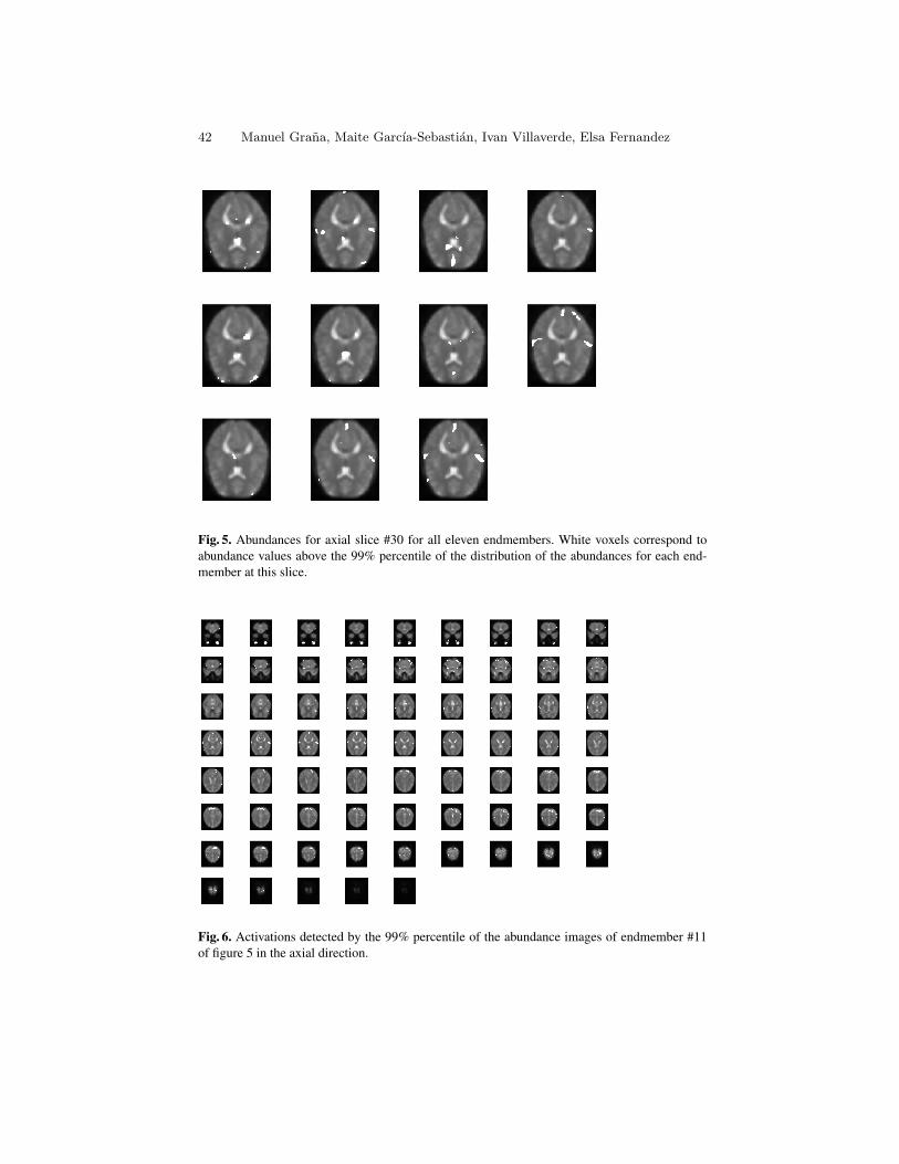
Fig. 5. Abundances for axial slice #30 for all eleven endmembers. White voxels correspond toabundance values above the 99% percentile of the distribution of the abundances for each end-member at this slice.

Fig. 6. Activations detected by the 99% percentile of the abundance images of endmember #11of figure 5 in the axial direction.


6 Conclusions and Discussion

We have proposed and applied the endmember induction algorithm EIHA discussed in[3] to the task of brain region activation in fMRI. The idea is to try to mimic ICA appli-cation to fMRI activation detection [1,13], where the sources correspond to endmem-bers detected by the EIHA algorithm and the activation is computed as the abundanceimages obtained by unmixing the voxel time series on the basis of the found endmem-bers. The first obstacle that we find in this endeavor is that the distribution of the timeseries is not well aspected for the detection of Lattice Independence as a meaningfulcharacteristic. In fact the voxel’s fMRI time series show a dense distribution of inten-sity displacements from the origin, so almost all of them are lattice dependent and ourproposed algorithm only recovers two endmembers. To overcome this problem we pro-pose a normalization which corresponds to a scale normalization in the sense of LatticeComputing. We substract its mean to each voxel time series. The resulting lattice nor-malized data set shows a much more rich structure in terms of Lattice Independence.Our computational experiment with a well known fMRI data set, provided with thedistribution of the SPM software, show some promising results in the sense that weare able to partially detect activations as the standard analysis with the SPM software.There are however some false detections that show that our approach is not consistentwith the SPM analysis. We think that further research may lead to obtain consistentresults. One important aspect of SPM is its process of the individual voxel t-test as arandom field, this processing is lacking in our initial works. Finding ways to harmo-nize global random field analysis and our lattice computing approach may lead to suchconsistency.

References

1. Calhoun, V.D.,Adali, T.: Unmixing fMRI with independent component analysis, Engineer-ing in Medicine and Biology Magazine, IEEE (2006) 25(2):79-90

2. Friston, K.J., Holmes, A.P., Worsley, K.J., Poline, J.P., Frith, C.D., Frackowiak, R.S.J.:Statistical parametric maps in functional imaging: A general linear approach, Hum. BrainMap. (1995) 2(4):189-210

3. Graña, M., Villaverde, I., Maldonado, J.O., Hernandez, C.: Two Lattice Computing ap-proaches for the unsupervised segmentation of Hyperspectral Images, Neurocomputing(2008) in press.

4. Graña, M.: A Brief Review of Lattice Computing, Proc. WCCI 2008, pp. 1777-17815. Muller, H.-P., Kraft, E., Ludolph, A., Erne, S.N.: New methods in fMRI analysis, Engineer-

ing in Medicine and Biology Magazine, IEEE, (2002) 21(5):134-1426. Pekar, J.J.: A brief introduction to functional MRI, Engineering in Medicine and Biology

Magazine, IEEE (2006) 25(2):24-267. Raducanu, B., Graña, M., Albizuri, X.: Morphological scale spaces and associative mor-

phological memories: results on robustness and practical applications, J. Math. Imagingand Vision (2003) 19(2):113–122

8. Ritter, G. X., Sussner, P., Diaz-de-Leon, J. L.: Morphological associative memories. IEEETrans. on Neural Networks, (1998) 9(2):281–292,

9. Ritter, G. X., Diaz-de-Leon, J. L., Sussner, P.: Morphological bidirectional associativememories. Neural Networks, (1999) 12:851–867,


10. Ritter, G.X., Urcid, G., Iancu, L.: Reconstruction of patterns from noisy inputs using mor-phological associative memories, J. Math. Imaging and Vision (2003) 19(2):95–112

11. Ritter, G.X., Gader, P., Fixed points of lattice transforms and lattice associative memoriesIn: Hawkes P (ed.) Advances in Imaging and Electron Physics (2006) 144:165–242, Else-vier, San Diego, CA

12. Ritter, G.X., Urcid, G., Schmalz, M.S.: Autonomous single-pass endmember approximationusing lattice auto-associative memories Neurocomputing (2008) in press

13. Sarty, G.E.: Computing Brain Activation Maps from fMRI Time-Series Images, CambridgeUniversity Press, 2007

14. Strother, S.C., Evaluating fMRI preprocessing pipelines, Engineering in Medicine and Bi-ology Magazine, IEEE (2006) 25(2):27-41


Redundant Encoding of Patternsin Lattice Associative Memories

Gonzalo Urcid1,?, Gerhard X. Ritter2, and Jose-Angel Nieves-V.1

1 Optics Department, INAOE, Tonantzintla, Pue. 72000, Mexicogurcid,[email protected]

2 CISE Department, University of Florida,Gainesville, FL 32611–6120, USA

[email protected]

Abstract. Lattice matrix auto-associative memories also known as auto-associative morphological memories are artificial neural networks used tostore and recall a finite set of binary or real valued patterns. They differfrom other auto-associative memory models in the way exemplar patternsare encoded in the network as well as in the computation performed torecall a pattern. Both storage and recall mechanisms are based on min-imax algebra operations that result in unique memory properties, suchas, single step recall, perfect retrieval of all exemplar patterns, and infi-nite storage capacity. Two dual lattice matrix auto-associative memorieshave been developed so far. The min-memory is robust to erosive noiseand the max-memory is robust to dilative noise; however, neither of thesememories is able to recall patterns degraded by mixed or random noise.This paper introduces a redundant encoding of patterns based on thegeometrical characterization of the set of fixed points common to bothmemories. Redundancy changes the size and shape of attraction basinsof exemplar patterns and expands the set of fixed points, hence recallcapability of patterns corrupted with random noise is possible using asimple scheme based on this type of memory networks.

Key words: Fixed point sets, Lattice associative memories, Minimaxalgebra, Morphological associative memories, Noisy patterns, Pattern re-call, Redundant encoding

1 Introduction

Lattice matrix auto-associative memories approach the problem of pattern asso-ciation from a minimax point of view. The Hebbian law of correlation encodingis still used to store a set of patterns but modified accordingly to be consis-tent with the mathematical framework of minimax algebra. Pattern retrievalis performed with minimax matrix products in a similar way as usual matrixmultiplication of linear algebra is used in linear correlation associative memorymodels. Brief but complete summaries of the different developments in the field? Corresponding author. Fax: +52 (222) 247-2940; Tel.: +52 (222) 266-3100 Ext.8205


of morphological associative memories can be consulted in [6, 10, 17, 18, 23]. Morerecently, the canonical lattice auto-associative memories (LAMs), also known asauto-associative morphological memories(AMMs), have been treated within themore general framework of lattice transforms. In this framework, the min-WXX

and max-MXX auto-associative memories are examples of lattice transforms be-tween n-dimensional real vectors. The set of fixed points of a lattice transformis a key concept since it provides a complete description of the transform behav-ior. Fixed points of AMMs where first presented in [15] and discussed further in[10, 18]; one of the main results is that WXX and MXX, have the same set offixed points denoted by F (X). Recently, an algebraic as well as a geometricalcharacterization of the set of fixed points F (X) has been established in [10, 12].This work proposes to exploit the infinite storage capacity and to take advantageof the geometrical nature of F (X), to enable recall capability of lattice matrixauto-associative memories for input patterns degraded by random noise.

Our work in the present paper is organized as follows: Section 2 provides thenecessary matrix operations borrowed from minimax algebra for dealing withlattice matrix associative memories. Also, an abstract overview of the main the-oretical results obtained from previous research on lattice auto-associative mem-ories is given very briefly. Section 3 describes the redundant encoding techniqueand simple examples with small sized matrix associative memories are given tomake explicit its potential. Section 4 presents some computational experimentswith a set of high-dimensional patterns, consisting of gray-scale images, thatdemonstrate the recall capability of canonical LAMs or AMMs when presentedwith noisy inputs. Finally, conclusions of this research are given in Section 5.


Mathematical definitions and key results about lattice matrix associative mem-ories are given here to support the geometrical encoding technique described inthe next section. For further material on the mathematical basis the reader isinvited to read previous works on the subject [4, 10, 18]. Computation in morpho-logical neural networks is performed within a mathematical framework that isbased on lattice algebra systems [1, 13]. More specifically, the extended real min-imax algebra [2, 5], denoted by (IR±∞,∧,∨,+,+′), is used for lattice associativememories where IR±∞ = IR ∪ −∞,+∞, the binary operations ∧,∨ denote,respectively, the min and max arithmetical operations between two numbers,and +,+′ correspond respectively, to addition and dual addition of arbitraryelements in IR±∞. For finite values x, y ∈ IR, we have that x+y = x+′ y. Matrixcomputations in minimax algebra are defined elementwise in a similar way asmatrix computations are defined in linear algebra. Two fundamental minimaxmatrix operations are matrix conjugation and matrix max-multiplication; givena matrix A of size m × p and a matrix B of size p × n over R±∞, for each

46 Gonzalo Urcid, Gerhard X. Ritter, Jose-Angel Nieves-V.

i = 1, . . . ,m and j = 1, . . . , n, they are defined as (t denotes transposition)

a∗ij = −aji or A∗ = −At (1)

cij =p∨

k=1

(aik + bkj) or C = A∨B. (2)

Dually, the min-product of matrices A and B, denoted by A∧B, is definedin terms of the generalized ∧-min operation. There are two canonical latticematrix associative memories known as the min-memory, denoted by WXY, andthe max-memory, denoted by MXY. Following a minimax correlated weight rule,each memory stores a set of k associations (xξ,yξ), represented by (X, Y ), whereX = (x1, . . . ,xk) ⊂ IRn and Y = (y1, . . . ,yk) ⊂ IRm. Left equations in (3) and(4) are given in entry format for i = 1, . . . ,m and j = 1, . . . , n; right equationsare in matrix notation.

wij = (WXY)ij =k∧

ξ=1

(yξi − xξ

j) ; WXY = Y ∨X∗ (3)

mij = (MXY)ij =k∨

ξ=1

(yξi − xξ

j) ; MXY = Y ∧X∗ (4)

If Y 6= X then a memory is called hetero-associative, otherwise it is calledauto-associative; this last case is where our attention is focused in this paper.We repeat two fundamental results on lattice auto-associative memories provedin [4]. First, WXX and MXX give perfect recall for perfect input in the sensethat, WXX ∨ xξ = xξ (resp. MXX ∧ xξ = xξ) for ξ = 1, . . . , k. Second, sincethe value of k is not restricted in anyway, WXX and MXX have infinite storagecapacity.

Missing parts, occlusions or corruption of exemplar patterns can be consid-ered as “noise” and we speak of random noise, when alterations in pattern entriesfollow a probability density function. Recall capabilities of LAMs for non-perfectinputs, requires noise to be classified in three basic types. Let I = 1, . . . , nthen, a distorted version x of pattern x has undergone an erosive change when-ever x ≤ x or equivalently if ∀i ∈ I, xi ≤ xi. A dilative change occurs wheneverx ≥ x or equivalently if ∀i ∈ I, xi ≥ xi. Let L,G ⊂ I be two non-empty disjointsets of indexes. If ∀i ∈ L, xi < xi and ∀i ∈ G, xi > xi, then the distorted patternx is said to contain mixed noise (random or structured). In practical situations,the “perfect recall” requirement is relaxed, and we say that WXX (resp. MXX)is an almost perfect recall memory for a set X of patterns if and only if thereexists a small rational number ε > 0 close to zero, such that µ(WXX ∨ x,x) ≤ ε(resp. µ(MXX ∧ x,x) ≤ ε) for all x ∈ X with respect to finite sets of noisyversions x of x, where µ(·) is an adequate measure tailored to treat with binaryor real valued patterns.

Redundant Encoding of Patterns in Lattice Associative Memories 47

The lattice matrix auto-associative memories WXX and MXX can be viewedas lattice transforms of the real vector space IRn into itself [5, 10, 24]. Thus, forexample, the min-memory is considered as a map WX : IRn → IRn for whichWX(x) = WXX ∨x for each x ∈ IRn. Sometimes, to simplify notation we writeW for the min-memory lattice transform instead of WX, if reference to the set Xis understood in the context of discourse. The natural factorization of the mapW , shown below in commutative diagram format, provides in a compact waythe action that W performs on input vectors.

IRn

π

W // IRn

IRn/RWη // ImW(IRn)

ι

OO (5)

In diagram (5), π : IRn → IRn/RW is the projection map (surjective) fromthe lattice transform domain IRn to the quotient set IRn/RW obtained from theinduced equivalence relation RW between pairs of n-dimensional vectors, i.e.,vector x is related to vector y if and only if W (x) = W (y). Let W (x) = x,then W (y) = x means that y is attracted to the fixed point x; otherwise, letW (x) = x′ 6= x, then W (y) = x′ and since x′ = W (x′) (one-step output re-call), y is attracted to another fixed point x′. The new fixed point x′ is simplya minimax combination of the exemplar patterns xξ ∈ X, a fact established in[10, 18]. The natural map (bijective), η : IRn/RW → ImW(IRn) establishes a oneto one and onto correspondence between each equivalence class ΩW(x) and thesingle image value W (x′) computed by W on each x′ ∈ ΩW(x). The equivalenceclass ΩW(x) corresponds to the orbit or attraction basin of a given input patternx; note that the input pattern may be an exemplar pattern xξ ∈ X and thatx′ may be a corrupted version xξ of xξ. The fact that ImW(IRn) equals the setof fixed points of the W transform was proved in [10], it is denoted by F (X)or alternatively by F (W ) = F (WX). It turns out that F (X) coincide for bothauto-associative memories, i.e., F (X) = F (W ) = F (M), and consists of the sameelements that belong to the linear minimax span of X. Under the natural mapη, the inverse image of any fixed point x gives its orbit, i.e., η−1(x) = ΩW(x).Finally, ι : F (X) → IRn is just an immersion map (injective) that assigns eachfixed point to itself within the original range of the W map.

To illustrate the previous ideas, we describe a simple example in detail for atwo-dimensional memory that stores just one pattern, i.e., let X = x1 wherex1 = (x1

1, x12) ∈ IR2; then, the min-memory matrix WXX is given by

WXX =(

w11 w12

w21 w22

)=

(0 w12

w21 0

). (6)

Without loss of generality we take x11 > x1

2, thus w12 = x11 − x1

2 > 0, w21 =x1

2 − x11 < 0, and w21 = −w12. There is no need to verify that WXX ∨x1 = x1,

since this is a specific instance of the perfect recall property that lattice auto-associative memories have on X [4]. Another useful result is that each column


vector of the matrix WXX is also a fixed point (a proof based on graph theoreticalconcepts appears in [18], for an alternative shorter argument see the Appendix).The recall stage for an input vector is explained next. Let x = (x1, x2) be aninput vector different to the stored exemplar pattern x1, i.e., x 6= x1 as shownin Fig. 1.

1x

2x

1x

2x

1

1x

1

2x

x

1x

12w

21w

1x

2x

1x

2x

1

1x

1

2x

x

1x

12w

21w

L( )x1

WM(.)

WM(.)

WW(.)

WW(.)

Fig. 1. The solid line L(x1) of slope 1 equals F (X), the set of fixed points of themin-WX transform for X = x1. In the diagram, x1, x ∈ F (X) but x 6= x1; the leftand bottom half rays form a single orbit under W , the upper and right half rays forma single orbit under M , and the arrows show the sense of attraction towards L(x1)

The entries of the output vector y recalled with the min-memory are com-puted as

y1 = (w11 + x1) ∨ (w12 + x2) = x1 ∨ (x11 − x1

2 + x2), (7)y2 = (w21 + x1) ∨ (w22 + x2) = x2 ∨ (x1

2 − x11 + x1). (8)

Consider the first coordinate y1 of the recalled pattern (abscissa of the newpoint) and let x2 = x1

2 (same vertical position), then

y1 = x11 ⇔ x1 < x1

1 (9)or y1 = x1 ⇔ x1 > x1

1, (10)

similarly, for the second coordinate y2 of the recalled pattern (ordinate of thenew point), let x1 = x1

1 (same horizontal position), hence

y2 = x12 ⇔ x2 < x1

2 (11)or y2 = x2 ⇔ x2 > x1

2. (12)


From (9) and (11), the orbit of the fundamental memory x1, denoted byΩW(x1), consists of all those points of IR2 that lie in the horizontal half-raydetermined by x1 ≤ x1

1 (eroded 1st coordinate) and x2 = x12, together with the

vertical half-ray determined by x1 = x11 and x2 ≤ x1

2 (eroded 2nd coordinate).Note that, less than or equal signs are used since x1 is included in the orbit,therefore

ΩW(x1) = x ∈ IR2|x1 ≤ x11, x2 = x1

2 ∪ x ∈ IR2|x1 = x11, x2 ≤ x1

2. (13)

On the other hand, from (10) and (12), if the abscissa of the input patternx ∈ IR2 is strictly to the right of x1

1 with x2 = x12, or its ordinate is strictly

above x12 with x1 = x1

1, then the recalled pattern is a fixed point different to thestored exemplar. Hence, x 6= x1 is such that WXX ∨x = x, or equivalently,

x1 = x1 ∨ (w12 + x2) and x2 = x2 ∨ (w21 + x1), (14)

which are satisfied, respectively, if x2 = w21 + x1 and x1 = w12 + x2.However, each one of the last two expressions implies the other by the fact,stated earlier, that w21 = −w12. Therefore, the coordinates of any new fixedpoint x 6= x1 are related by a single linear equation given by

x2 = x1 + w21, (15)

which is a line of positive slope equal to 1 and intercept at the origin equal tow21. The line passing through the points (0, w21), (x1

1, x12) = x1, and (x1, x2) = x,

is denoted by L(x1), to remind its relation to the exemplar pattern x1 ∈ X.Hence, the min-memory matrix transformation WX has an infinite number offixed points x 6= x1, such that x ∈ L(x1), and the whole plane IR2 is partitionedthrough their orbits, i.e.,

IR2 =⋃ΩW(x) | x ∈ L(x1). (16)

A similar analysis can be carried out for the max-memory transform MX

with X = x1. Although, the fixed points of M lie on the same line L(x1), theorbit of the fundamental memory x1, ΩM(x1) 6= ΩW(x1), since it is composedof points that lie in the horizontal half-ray determined by x1 ≥ x1

1 (dilated1st coordinate) and x2 = x1

2, together with the vertical half-ray determined byx1 = x1

1 and x2 ≥ x12 (dilated 2nd coordinate), hence

ΩM(x1) = x ∈ IR2|x1 ≥ x11, x2 = x1

2 ∪ x ∈ IR2|x1 = x11, x2 ≥ x1

2. (17)

Also, ΩW(x) ∩ ΩM(x) = x for any x ∈ L, and the dual partition of theplane IR2 is given by

⋃ΩM(x) | x ∈ L(x1). We remark that, the line given in

(15) can be obtained directly from the WXX matrix. Here, W1XX = (0, w21)t is

the intercept point on the x2 axis and W2XX = (w12, 0)t is the intercept point on

the x1 axis. These two points, depicted as hollow dots on Fig. 1, define L. For thisexample, given a distorted version of x1, denoted by x1, the min-memory WXX

(resp. max-memory MXX) is capable of perfect recall, i.e., WXX ∨ x1 = x1 (resp.MXX ∧ x1 = x1), if and only if x1 ∈ ΩW(x1) (resp. x1 ∈ ΩM(x1)), meaning thatx1 must be eroded (resp. dilated) in one of its two coordinates but not both.


3 Redundant Encoding

Besides the algebraic characterization given for F (X) in the previous section, ageometrical characterization of the set of fixed points has been recently devel-oped in [10, 12]. The shape of F (X) corresponds to an m-dimensional convexprismatic beam with 1 ≤ m ≤ n, and the value of m depends on the nature ofthe underlying finite set X of exemplar pattern vectors. Schematic visualizationof the set F (X) is possible only for n = 1, 2, 3; for higher dimensions, used ismade of concepts from n-dimensional geometry of which the necessary materialtogether with a detailed treatment of the shape of F (X) appears in [10, 12].Simple numerical examples in lower dimensions (small sized memories) makeevident the inherent limitations of any lattice matrix auto-associative memory,in the sense that, neither WXX nor MXX is able to recall correctly any exem-plar pattern that has been corrupted with random noise. Also, the surprisingrobustness of the min-memory WXX with respect to erosive noise as well asthe max-memory MXX against dilative noise is related to typical applicationswhose patterns are points in higher dimensional spaces, i.e., for ξ = 1, . . . , k,xξ ∈ IRn with n 1. Complementary theoretical developments coupled withcomputational techniques such as the kernel methods [3, 4, 6, 14, 16, 21], fuzzyMAM models [19, 20, 25], enhanced memory schemes [22, 26], and dendrite basedmodels [7–11], offer alternative solutions to robust pattern recall from noisyinputs. Recently, the technique of noise masking has been introduced to takeadvantage of the strong properties that single lattice matrix auto-associativememories have [23]. All the previous techniques share in common an increase incomputational complexity or in the definition of the network topology; however,none of them exploits the infinite storage capacity property that WXX and MXX

have. Therefore, we propose to use the aforementioned property together withthe geometrical characterization of the fixed point set of LAMs, to introduce asimple procedure based on redundant encoding, to enable the recall of patternapproximations to exemplars from distorted inputs.

Given a set X = x1,x2, . . . ,xk of k exemplar patterns xξ, with finite realentries, redundant encoding consists in the storage of additional, carefully designpatterns to set X. The new patterns must be spatially related to the original onesand for each xξ ∈ X, with ξ = 1, . . . , k, the same number p of related patterns,denoted by xξ1 ,xξ2 , . . . ,xξp, can be stored in the new min- and max-memoriesdefined on the augmented set XG given by

XG = X ∪k⋃

ξ=1

p⋃q=1

xξq (18)

If |X| = k then |XG| = k(p+1) which poses no problem, since W and M haveinfinite storage capacity. The purpose to add redundant patterns to the originalexemplar pattern set X is to increase the number of fixed points by changing thegeometrical shape of F (X), and to expand it, in the sense that F (XG) ⊃ F (X).It is essential for this scheme to work that the new encoded patterns includeerosive and dilative, or mixed approximations of each exemplar pattern. In other


words, lattice matrix auto-associative memories should remember not only theexemplars but also some eroded and dilated, or mixed resemblances of them.This simple mechanism endows them with recall capability in the presence ofarbitrary noisy inputs. In what follows, we consider the minimum redundantcase, in which only a single approximate pattern is considered for each exemplar.Thus, p = 1 and only 2k patterns, x1, . . . ,xk,x11, . . . ,xk1, are stored in theaugmented memories, WXGXG and MXGXG .

To illustrate the basic idea behind the proposed technique, we elaboratefurther the example provided in Section 2. Thus, if set X has a single patternx such that x1 = x2, then line L(x) passes through the origin, and contains allthe fixed points of the min- and max-transforms WX and MX, i.e., F (X) = L(x)as shown by the dotted line at 45 with respect to the x1 axis in Fig. 2. Thepoints to the left, right, below, and above, respectively, denoted by, x`,xr,xb,and xa, represent close approximations to the exemplar pattern x. For ε > 0,let the coordinates of these points be defined by x` = (x`

1, x`2) = (x1 − ε, x2),

xr = (xr1, x

r2) = (x1 + ε, x2), xb = (xb

1, xb2) = (x1, x2 − ε), and xa = (xa

1 , xa2) =

(x1, x2 + ε). Also, notice that, x` and xb are eroded, respectively, in its 1stand 2nd coordinates; similarly, xr and xa are dilated, respectively, in x1 andx2. Although we can adjoin all four points to X to build the augmented setXG, the addition of only two points not on the same line, such as x`,xr,xa,xb, x`,xb, or xa,xr, give the same set of fixed points for XG. LetXG = x,xa,xr, then the lattice auto-associative memories of XG, computedfrom (3) and (4), are given by

WXGXG =(

0 −ε−ε 0

)and MXGXG =

(0 εε 0

). (19)

Alternatively, the max-memory matrix can be computed using the fact thatM = W∗ together with (1). Next, to determine F (XG), we solve the equationWXGXG ∨x′ = x′ for x′ not in XG, equivalently, x′i =

∨2j=1(wij+x′j) for i = 1, 2.

The resulting expressions are given by x′1 = x′1 ∨ (x′2− ε) and x′2 = x′2 ∨ (x′1− ε),from which x′2 − ε ≤ x′1 and x′1 − ε ≤ x′2, consequently, x′1 − ε ≤ x′2 ≤ x′1 + ε.The boundary values for x′2 in this last compound inequality provide us withthe line equations of slope 1, x′2 = x′1 + ε and x′2 = x′1 − ε, labeled in Fig. 2as La = L(xa) and Lr = L(xr), respectively. Since x′2 ∈ [x′1 − ε, x′1 + ε], thefixed point set of XG consists of all points that belong to La and Lr, or liein the infinite band between them. Mathematically, if H−

a denotes the closedhalf plane on and below the line La and H+

r denotes the closed half plane onand above the line Lr, then, F (XG) = H−

a ∩ H+r . Notice that, by definition,

H+a ∩ H−

a = La and H+r ∩ H−

r = Lr, hence the boundary of the fixed pointset of XG is given by ∂F (XG) = La ∪ Lr. The geometric shape of F (X) forn-dimensional patterns is fully developed in [12]. In this example, by encodingtwo redundant patterns that are spatially related to the single exemplar in X,an expanded fixed point set is obtained such that F (X) ⊂ F (XG). For patternrecall in the presence of noise, we may consider all fixed points x′ ∈ F (XG)that satisfy the inequality, |x′1 − x1|+ |x′2 − x2| ≤ ε (hatched rhombus shown in


Fig. 2), to be “good” approximations to a given exemplar pattern x, in the sensedescribed earlier for almost perfect recall using a single lattice auto-associativememory. The parameter ε gives us the possibility to increase or decrease thesize of the rhombus shaped neighborhood and therefore to relax or constrain theadmissible memory outputs.

1x

2x

2

lx

1

bx

2

bx

x

bx

rL

1

lx

lx

aL

rx

ax

1

rx

2

ax

1x

2x

2

lx

1

bx

2

bx

x

bx

rL

1

lx

lx

aL

rx

ax

1

rx

2

ax

L( )x

WM(.)

WW(.)

WM(.)

WW(.)

e

-e

e

-e

Fig. 2. The solid line L(x) of slope 1 equals F (X), the set of fixed points of the min-WX transform for X = x. The points, x`, xr, xa, xb ∈ F (XG) are eroded or dilatedversions of x in a single coordinate. The left and bottom half rays are different orbitsunder WXG , the upper and right half rays are distinct orbits under MXG , and thearrows show the sense of attraction, respectively, towards La or Lr

It is reasonable to expect that for high dimensional patterns, redundant en-coding can be achieved in various ways. The extension of the base examples,described previously, to higher dimensions (n > 3) is impossible to visualize.However, the basic procedure is still the same, since a subset of the coordinatesof a given exemplar pattern in X can be eroded to a minimum prescribed valueand another subset of coordinates, disjoint from the first, may be dilated to amaximum prescribed value. The rest of the coordinate values would remain thesame as those in the original exemplar. In this manner, a single redundant pat-tern related spatially to each exemplar in X is encoded to build XG. Adjoinedpatterns are then approximations to exemplars which also can be regarded as“noisy” versions of them, in the sense that, mixed structured noise is inducedby eroding and dilating several coordinates. Clearly, the adequate selection ofthe coordinate subsets to be modified is determined by pattern dimensionalityas well as their nature in a given application.


4 Application Example

To test our proposal, we conducted a computer experiment using 10 gray scaleimages of size 53×53 pixels as integer valued patterns of dimension 2809. Fig. 3displays only four of these exemplar pattern images together with a single re-dundant encoded pattern obtained by assigning a minimum value (0 for extremeerosion) or a maximum value (255 for extreme dilation) to the gray values of asubset of the pixel coordinates, the same for each exemplar in X. Hence, using(3) and (4), the memory matrices WXGXG and MXGXG , of size 2809 × 2809,store all associations between the 20 patterns in the augmented set XG.

Fig. 3. 1st row: exemplar patterns x1, x3, x6, x8 ∈ X; 2nd row: redundant encodedpatterns x11, x31, x61, x81 adjoined to X to form XG; 3rd row: noisy versions of ex-emplars, respectively, with noise probabilities of 0.3, 0.4, 0.5, and 0.6; 4th row: recalledpattern approximations.

Each pattern in X was contaminated 100 times by adding random noise withprobabilities 0.1 to 0.9 and 128 as offset value. The measure µ(·) used for almostperfect recall is the normalized mean square error (NMSE) defined by σ(x, x) =∑n

i=1(xi − xi)2/∑n

i=1 x2i . Fig. 4 shows the performance curves obtained in the

recall stage using as final output, the arithmetical mean of the min and maxmemory outputs, since WXGXG attracts points towards F (XG) by increasingcoordinate values and MXGXG attracts points towards F (XG) by decreasingcoordinate values. Also, if more and more pattern entries are affected by noise,these modified entries are less likely to be equal in the remaining patterns, thusit is no surprise that NMSE decreases as the probability of error increases. Inspite of this abnormal behavior, adjoining redundant encoded patterns to the


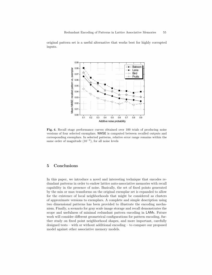
original pattern set is a useful alternative that works best for highly corruptedinputs.

0.1 0.2 0.3 0.4 0.5 0.6 0.7 0.8 0.9

0.00

0.01

0.02

0.03

0.04

0.05

0.06

0.07

0.08

0.09

Mean

NM

SE

:re

calle

dpattern

vs.exe

mpla

r

Additive noise probability

BaboonLenaBirdFruits

Fig. 4. Recall stage performance curves obtained over 100 trials of producing noiseversions of four selected exemplars. NMSE is computed between recalled outputs andcorresponding exemplars. In selected patterns, relative error range remains within thesame order of magnitude (10−2), for all noise levels

5 Conclusions

In this paper, we introduce a novel and interesting technique that encodes re-dundant patterns in order to endow lattice auto-associative memories with recallcapability in the presence of noise. Basically, the set of fixed points generatedby the min or max transforms on the original exemplar set is expanded to allowfor the existence of local neighborhoods that might be considered as clustersof approximate versions to exemplars. A complete and simple description usingtwo dimensional patterns has been provided to illustrate the encoding mecha-nism. Finally, a scenario for gray scale image storage and recall demonstrates thescope and usefulness of minimal redundant pattern encoding in LAMs. Futurework will consider different geometrical configurations for pattern encoding, fur-ther study on fixed point neighborhood shapes, and more important, carefullydesigned tests – with or without additional encoding – to compare our proposedmodel against other associative memory models.


Appendix

Theorem 1. Let X = (x1, . . . ,xk) ⊂ IRn be a set of k exemplar patterns andlet (w1, . . . ,wλ, . . . ,wn) denote the column vectors of the corresponding min-memory WXX of size n× n, then WXX ∨wλ = wλ for λ = 1, . . . , n. Therefore,any column of the matrix WXX is a fixed point for the min-memory transform.

Proof. By definition, the entries of the column vector wλ of WXX for j = 1, . . . , nare given by wλ

j =∧k

ξ=1(xξj−xξ

λ), and the entries of the recalled output pattern y

are computed as follows, yi = (WXX ∨wλ)i =∨n

j=1(wij+wλj ) = wλ

i ∨∨

j 6=i(wij+wλ

j ), for i = 1, . . . , n. Since, for all i, wij + wjλ ≤ wiλ = wλi , by Lemma 5.1 in

[10], then∨

j 6=i(wij + wλj ) ≤ wλ

i ⇒ yi = wλi .

A similar result holds for the max-memory MXX, i.e., any column of the MXX

matrix is a fixed point for the max-memory transform. Since WXX ∨WXX =WXX and MXX ∧MXX = MXX, the previous result is equivalent to the fact thatWXX and MXX are idempotent, respectively, under the max and min products.

Acknowledgment

Gonzalo Urcid thanks the National Research System (SNI) and the NationalCouncil of Science and Technology (CONACYT) in Mexico for the partial supportprovided for this work under grant 22036. Jose A. Nieves-Vazquez also thanksCONACYT for doctoral scholarship 181663.

References

1. Birkhoff, G.: Lattice Theory 3rd ed, Am. Math. Soc., Providence RI (1967).2. Cuninghame-Green, R.: Minimax algebra and applications. In: Hawkes, P. (ed)

Advances in Imaging and Electron Physics, 90, Academic Press, New York (1995)1–121.

3. Hattori, M., Fukui, A., Ito, H.: A fast method of constructing kernel patterns formorphological associative memories. Proc. 9th Int. Conf. on Neural InformationProcessing, Singapore China (2002) 1058–1063.

4. Ritter, G.X., Sussner, S., Diaz de Leon, J.L.: Morphological associative memories.IEEE Trans. on Neural Networks, 9(2) (1998) 281–293.

5. Ritter, G.X.: Lattice algebra & Minimax algebra. In: Image Algebra, unpublishedmanuscript available via anonymous ftp, CISE Department, University of Florida,Gainesville FL (1999) 121–135.

6. Ritter, G.X., Urcid, G., Iancu, L.: Reconstruction of noisy patterns using mor-phological associative memories. J. of Math. Imaging and Vision, 19(5) (2003)95–111.

7. Ritter, G.X., Iancu, L.: A morphological auto-associative memory based on den-dritic computing. Proc. IEEE (2004) 915–920.

8. Ritter, G.X., Iancu, L.: Lattice algebra approach to neural networks and patternclassification. Pattern Recognition and Image Analysis, 14(2) (2004) 190–197.


9. Ritter, G.X., Urcid, G., Schmalz, M.S.: Lattice associative memories that are ro-bust in the presence of noise. SPIE Proc., Mathematical Methods in Pattern andImage Analysis, 5916, San Diego CA (2005) 59160Q1–Q6.

10. Ritter, G.X., Gader, P.: Fixed Points of Lattice Transforms and Lattice AssociativeMemories. In: Hawkes, P.(ed) Adv. in Imaging and Electron Physics, 144. Elsevier,San Diego CA (2006) 165–242.

11. Ritter, G.X., Urcid, G.: Learning in Lattice Neural Networks that Employ Den-dritic Computing. In: Kaburlasos, V.G. & Ritter, G.X.(eds) Computational Intel-ligence based on Lattice Theory, 67. Springer, Heidelberg, Germany (2007) 25–44.

12. Ritter, G.X., Urcid, G.: Fast autonomous endmember determination using latticealgebra, in preparation for IEEE Trans. on PAMI.

13. Skornjakov, L.A.: Elements of Lattice Theory, Adam Hilger, Bristol UK (1977).14. Sussner, P.: Observations on morphological associative memories and the kernel

method. Neurocomputing, 31 (2000) 167–183.15. Sussner, P.: Fixed points of autoassociative morphological memories. Proc. of the

Int. Joint Conf. on Neural Networks, Como, Italy (2000) 611–616.16. Sussner, P.: Associative morphological memories based on variations of the kernel

and dual kernel methods. Neural Networks, 16(5) (2003) 625–632.17. Sussner, P.: Recall of patterns using binary and gray-scale autoassociative mor-

phological memories. SPIE Proc., Mathematical Methods in Pattern and ImageAnalysis, 5916, San Diego CA (2005) 59160M:1-10.

18. Sussner, P., Valle, M.E.: Gray-scale morphological associative memories. IEEETrans. on Neural Networks, 17(3) (2006) 559–570.

19. Sussner, P., Valle, M.E.: Implicative fuzzy associative memories. IEEE Trans. onFuzzy Systems, 14(6) (2006) 793–807.

20. Sussner, P., Valle, M.E.: Fuzzy Associative Memories and Their Relationship toMathematical Morphology. In: Pedrycz, W., Skowron, A. & Kreinovich, V. (eds)Handbook of Granular Computing, Ch. 33, Wiley, (2008).

21. Urcid, G., Ritter, G.X.: Kernel computation in morphological associative memoriesfor gray-scale image recollection. Proc. 5th IASTED Int. Conf. on Signal and ImageProcessing, Honolulu HI (2003) 450–455.

22. Urcid, G., Nieves-V., J.A. Reyes-G, C.A.: Enhanced fuzzy autoassociative morpho-logical memory for binary pattern recall. Proc. 4th IASTED Int. Conf. on SignalProcessing, Pattern Recognition, and Applications, Innsbruck, Austria (2007) 116–121.

23. Urcid, G., Ritter, G.X.: Noise Masking for Pattern Recall using a Single LatticeMatrix Associative Memory. In: Kaburlasos, V.G. & Ritter, G.X.(eds) Computa-tional Intelligence based on Lattice Theory, 67. Springer, Heidelberg, Germany(2007) 79–98.

24. Urcid, G., Valdiviezo-N., J.C., Generation of lattice independent vector sets forpattern recognition applications. SPIE Proc., Mathematics of Data/Image PatternRecognition, Compression, Coding, and Encryption X with Applications,6700, SanDiego CA (2007) 67000C :1–12.

25. Valle, M.E., Sussner, P.: A general framework for fuzzy morphological associativememories. Fuzzy Sets and Systems, 159(7) (2008) 747–768.

26. Wang, M., Chen, S.: Enhanced fuzzy morphological auto-associative memory basedon empirical kernel map. IEEE Trans. on Neural Networks, 16(3) (2005) 557–564.


A Novel Fuzzy Implication Stemming from aFuzzy Lattice Inclusion Measure

Anestis G. Hatzimichailidis and Vassilis G. Kaburlasos

Technological Educational Institution of KavalaDepartment of Industrial Informatics

65404 Kavala, [email protected];[email protected]

Abstract. We introduce a fuzzy implication stemming from a fuzzylattice inclusion measure. We study “reasonable axioms” and propertiesof the aforementioned fuzzy implication, which (properties) are typicalyrequired in the literature and could be important in certain applications.

Key words: Fuzzy lattice theory, Fuzzy implications, Inclusion measure

1 Introduction

A number of basic properties of the classical (logic) implication have been gener-alized in fuzzy implications; hence, a number of “reasonable axioms” have beenproposed tentatively for fuzzy implications [10], [12].

Lately, an inclusion measure function was introduced in a mathematical lat-tice (L,≤) for fuzzying the corresponding (crisp) partial order relation [6], [8].In this paper we study a fuzzy implication stemming from the aforementionedinclusion measure. We show that the proposed fuzzy implication satisfies most ofthe “reasonable axioms” proposed in the literature. We study additional proper-ties of our proposed fuzzy implication. The latter properties are typicaly requiredin the literature and could be important in certain applications.

The layout is as follows. Section 2 presents mathematical preliminaries. Sec-tion 3 introduces a novel fuzzy implication. Section 4 concludes by summarizingthe contribution including also a description of potential future work.

2 Mathematical Preliminaries

This section presents basic notions of (Fuzzy) Lattice Theory and Fuzzy SetsTheory [2], [3], [6], [8], [10], [11].

2.1 Inclusion Measure

Consider the following definitions.

Definition 1. Given a set P, a binary relation (≤) on P is called partial orderif and only if it satisfies the following conditions for all x, y, z ∈ P:


PO1. Reflexivity: x ≤ x.PO2. Antisymmetry: x ≤ y and y ≤ x ⇒ x=y.PO3. Transitivity: x ≤ y and y ≤ z ⇒ x ≤ z.

Condition PO2 can be replaced by the following equivalent condition:

PO2′. Antisymmetry: x ≤ y and x 6= y ⇒ y x.

Definition 2. A partially ordered set, or poset for short, is a pair (P,≤),where P is a set and ≤ is a partial order relation on P .

Definition 3. A (crisp) lattice is a poset (L,≤) any two of whose elementshave both a greatest lower bound and a least upper bound. A lattice (L,≤) iscalled complete when each of its subsets X has both a greatest lower bound anda least upper bound in L.

Definition 4. Let (L,≤) be a complete lattice with least and greatest elements Oand I, respectively. An inclusion measure in (L,≤) is a map σ : L×L → [0, 1],which satisfies the following conditions for u, w, x ∈ L:

IM0. σ(x, O) = 0,∀x 6= OIM1. σ(x, x) = 1,∀x ∈ LIM2. u ≤ w ⇒ σ(x, u) ≤ σ(x,w) (Consistency Property)IM3. x ∧ y < x ⇒ σ(x, y) < 1

For a non-complete lattice condition IM0 is dropped.Based on equivalence relation x ∧ y < x ⇐⇒ y < x ∨ y ([1]) it follows that

condition IM3 can, equivalently, be replaced by

IM3′. y < x ∨ y ⇒ σ(x, y) < 1.

Conditions IM1 and IM2 imply u ≤ w ⇒ σ(u, u) ≤ σ(u, w) ⇒ σ(u, w) = 1,u, w ∈ L. Hence, σ(x, I) = 1, ∀x in a complete lattice (L,≤).

2.2 Fuzzy Implications

Let X be a universe of discourse. A fuzzy set A in X ([14]) is defined as a setof ordered pairs A = (x, µA(x)) : x ∈ X, where function µA : X → [0, 1]indicates the degree of membership of an element x ∈ X in fuzzy set A.

Definition 5. A binary operation i : [0, 1] × [0, 1] → [0, 1], is called fuzzy in-tersection if it is an extension of the classical Boolean intersection as follows

BI1. i(a, b) ∈ [0, 1], ∀a, b ∈ [0, 1], andBI2. i(0, 0) = i(0, 1) = i(1, 0) = 0; i(1, 1) = 1

A canonical model of fuzzy intersections is the family of triangular norms,or t-norms for short, defined rigorously next.

60 Anestis G. Hatzimichailidis, Vassilis G. Kaburlasos

Definition 6. A t-norm is a function i : [0, 1] × [0, 1] → [0, 1], which is com-mutative, associative, non-decreasing, and i(α, 1) = α, ∀α ∈ [0, 1].

A t-norm i is called Archimedean if it is both continuous and a ∈ (0, 1) impliesi(a, a) < a; furthermore, a t-norm i is called nilpotent if it is both continuousand ∀α ∈ (0, 1) there is a ν ∈ N such that i(a, . . . , a) = 0. Archimedean normsare either nilpotent or non-nilpotent. The latter (norms) are also called strict.

Definition 7. A function n : [0, 1] → [0, 1] is called negation if it is bothnon-increasing, i.e. n(a) ≤ n(b) for a ≥ b, and n(0) = 1, n(1) = 0.

A negation n is called strict if and only if n is both continuous and strictlydecreasing, i.e. n(a) < n(b) for a > b, ∀a, b ∈ [0, 1]. A strict negation n is calledstrong if and only if it is self-inverse, i.e. n(n(a)) = a, ∀a ∈ [0, 1]. The mostpopular strong negation is the standard negation: nS = 1− a.

A triangular conorm, or t-conorm, is a function u : [0, 1] × [0, 1] → [0, 1],which satisfies the following properties:

i) u(a, 0) = a, ∀a ∈ [0, 1],ii) u(a, b) ≤ u(c, d) if both a ≤ c and b ≤ d,iii) u(a, b) = u(b, a), ∀a, b ∈ [0, 1], andiv) u(u(a, b), c) = u(a, u(b, c)), ∀a, b, c ∈ [0, 1].

A fuzzy implication is a function g : [0, 1] × [0, 1] → [0, 1], which for anytruth values a, b ∈ [0, 1] of (fuzzy) propositions p, q, respectively, gives the truthvalue g(a, b) of conditional proposition “if p then q”. Function g(., .) should bean extension of the classical implication from domain 0, 1 to domain [0, 1].

The implication operator of classical logic is a map m : 0, 1×0, 1 → 0, 1which satisfies the following conditions: m(0, 0) = m(0, 1) = m(1, 1) = 1 andm(1, 0) = 0. The latter conditions are typically the minimum requirements fora fuzzy implication operator. In other words, fuzzy implications are required toreduce to the classical implication when truth-values are restricted to 0 and 1;i.e. g(0, 0) = g(0, 1) = g(1, 1) = 1 and g(1, 0) = 0.

2.2.1 Properties of fuzzy implications

One way of defining an implication operator m in classical logic is usingformula m(a, b) = a∨b, a, b ∈ 0, 1, where a denotes the negation of a. Another(equivalent) way of defining implication operator m in classical logic is usingformula m(a, b) = maxx ∈ 0, 1 : a ∧ x ≤ b, a, b ∈ 0, 1.

Fuzzy logic extensions of the previous formulas, respectively, are

g(a, b) = u(n(a), b) (1)

and

g(a, b) = supx ∈ [0, 1] : i(a, x) ≤ b, (2)

A Novel Fuzzy Implication Stemming from a Fuzzy Lattice Inclusion Measure 61

∀a, b ∈ [0, 1], where u, i and n denote a fuzzy union, a (continuous) fuzzyintersection, and a fuzzy negation, respectively. Note that functions u and i aredual (with respect to n) — Recall that a t-norm i and a t-conorm u are called dual(with respect to a fuzzy negation n) if and only if both n(i(a, b)) = u(n(a), n(b))and n(u(a, b)) = i(n(a), n(b)) hold ∀a, b ∈ [0, 1].

Fuzzy implications obtained from (1) are usually referred to as S-implications,whereas fuzzy implications obtained from (2) are called R-implications.

Formula m(a, b) = a∨b can also be rewritten, based on the law of absorptionof negation in classical logic, as either m(a, b) = a∨(a∧b) or m(a, b) = (a∧b)∨b.Extensions of the latter equations in fuzzy logic are given, respectively, by

g(a, b) = u(n(a), i(a, b)) (3)

and

g(a, b) = u(i(n(a), n(b)), b), (4)

where u, i and n are required to satisfy the De Morgan laws. The fuzzyimplications obtained from (3) are called QL-implications because they wereoriginally introduced in quantum logic.

A number of basic properties of the classical (logic) implication have beengeneralized by fuzzy implications. Hence, a number of “reasonable axioms”emerged tentatively for fuzzy implications. Some of the aforementioned axiomsare displayed next [10], [12].

A1. a ≤ b ⇒ g(a, x) ≥ g(b, x) Monotonicity in first argumentA2. a ≤ b ⇒ g(x, a) ≤ g(x, b) Monotonicity in second argumentA3. g(a, g(b, x)) = g(b, g(a, x)) Exchange Property

This is a generalization of the equivalence between a ⇒ (b ⇒ x) and b ⇒(a ⇒ x) in classical implication.

A4. g(a, b) = g(n(b), n(a)) ContrapositionA5. g(1, b) = b Neutrality of truthA6. g(0, a) = 1 Dominance of falsityA7. g(a, a) = 1 IdentityA8. g(a, b) = 1 ⇐⇒ a ≤ b Boundary ConditionA9. g is a continuous function Continuity

We remark that one can easily prove that a S-implication fulfills axiomsA1, A2, A3, A5, A6 and, when negation n is strong, it also fulfills axiom A4.Furthermore, a R-implication fulfills axioms A1, A2, A5, A6, and A7.

3 A Novel Fuzzy Implication

An inclusion measure (σ) can be used to quantify partial (fuzzy) set inclusion. Inthis sense σ(x, y) is similar to alternative definitions proposed in the literature forquantifying a degree of inclusion of a (fuzzy) set into another one [6]. However,the aforementioned “alternative” definitions typically involve only overlapping


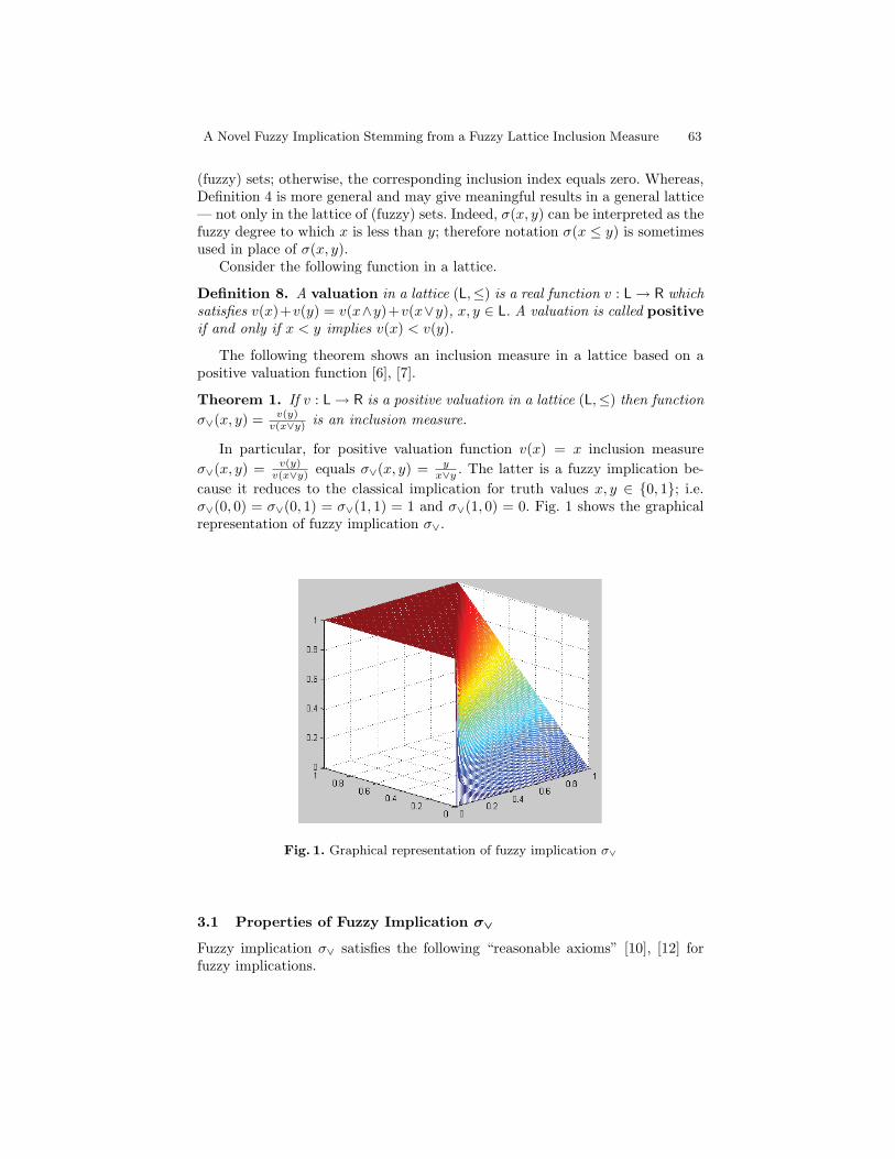
(fuzzy) sets; otherwise, the corresponding inclusion index equals zero. Whereas,Definition 4 is more general and may give meaningful results in a general lattice— not only in the lattice of (fuzzy) sets. Indeed, σ(x, y) can be interpreted as thefuzzy degree to which x is less than y; therefore notation σ(x ≤ y) is sometimesused in place of σ(x, y).

Consider the following function in a lattice.

Definition 8. A valuation in a lattice (L,≤) is a real function v : L → R whichsatisfies v(x)+v(y) = v(x∧y)+v(x∨y), x, y ∈ L. A valuation is called positiveif and only if x < y implies v(x) < v(y).

The following theorem shows an inclusion measure in a lattice based on apositive valuation function [6], [7].

Theorem 1. If v : L → R is a positive valuation in a lattice (L,≤) then functionσ∨(x, y) = v(y)

v(x∨y) is an inclusion measure.

In particular, for positive valuation function v(x) = x inclusion measureσ∨(x, y) = v(y)

v(x∨y) equals σ∨(x, y) = yx∨y . The latter is a fuzzy implication be-

cause it reduces to the classical implication for truth values x, y ∈ 0, 1; i.e.σ∨(0, 0) = σ∨(0, 1) = σ∨(1, 1) = 1 and σ∨(1, 0) = 0. Fig. 1 shows the graphicalrepresentation of fuzzy implication σ∨.

Fig. 1. Graphical representation of fuzzy implication σ∨

3.1 Properties of Fuzzy Implication σ∨

Fuzzy implication σ∨ satisfies the following “reasonable axioms” [10], [12] forfuzzy implications.


Proposition 1. Consider fuzzy implication σ∨. Let a, b, x ∈ [0, 1]. Then

A1. a ≤ b ⇒ σ∨(a, x) ≥ σ∨(b, x)A2. a ≤ b ⇒ σ∨(x, a) ≤ σ∨(x, b)A3. σ∨(a, σ∨(b, x)) = σ∨(b, σ∨(a, x))A4′. σ∨(a, b) = σ∨(n(b), n(a)) — see in the following remarkA5. σ∨(1, b) = bA6. σ∨(0, a) = 1A7. σ∨(a, a) = 1A8. σ∨(a, b) = 1 ⇐⇒ a ≤ bA9. σ∨ is a continuous function

We remark that axioms (A1) − (A3) and (A5) − (A9) in Proposition 1 canbe proved immediately. For the standard fuzzy complement n(a) = 1−a, axiom(A4) holds only if a ≤ b; whereas, for a > b, axiom (A4) holds only if a + b = 1.

Additional “reasonable axioms” [13] include the following.

A10. g(a, i(b, c)) = i(g(a, b), g(a, c))A11. i(g(a, b), g(n(a), b)) = bA12. i(g(0.5, b), g(0.5, b)) = bA13. g(a, g(b, c)) = g(i(a, b), c)

The next proposition shows how fuzzy implication σ∨ satisfies axioms (A10)-(A13) (with the “min” operator (∧) employed as a fuzzy t-norm).

Proposition 2. Consider fuzzy implication σ∨. Let a, b, c ∈ [0, 1]. Then

A10. σ∨(a, (b ∧ c)) = ∧(σ∨(a, b), σ∨(a, c))A11′. ∧(σ∨(a, b), σ∨(n(a), b)) > bA12′. ∧(σ∨(0.5, b), σ∨(0.5, b)) > bA13′. σ∨(a, σ∨(b, c)) = σ∨(∧(a, b), c), for c ≥ a ∧ b.

Proposition 2 can be proved immediately.The following propositions describe some properties of fuzzy implication σ∨,

which (properties) are often required in the literature because they could beimportant in certain applications [5], [10], [11].

Proposition 3. Let us denote σ∨(a, b) by a → b. Then

i) (a ∧ b) → c = (a → c) ∨ (b → c)ii) (a ∨ b) → c = (a → c) ∧ (b → c)

Proposition 3 can be proved immediately.

Proposition 4. Consider both fuzzy implication σ∨ and the standard negationnS = 1− a (a′ for short). Then

i) σ∨(a, 1) = 1, ∀a ∈ [0, 1]ii) σ∨(σ∨(a, b), c) ≤ σ∨(a, σ∨(b, c)), ∀a, b, c ∈ [0, 1]iii) ∨(a, σ∨(a, b)) = σ∨(a,∨(b, c)), for a ≤ b


iv) ∧(a, σ∨(a, b)) ≤ b, for a ≤ bv) σ∨(a, a′) > a′, ∀a ∈ [0, 1]vi) σ∨(a′, a) > a, ∀a ∈ [0, 1]vii) (σ∨(a, b))′ ≤ σ∨(a′, b′), ∀a, b ∈ [0, 1]viii) σ∨(a, b) ≥ b, ∀a, b ∈ [0, 1]ix) σ∨(a, b) ≥ a′, for a ≤ b


Proposition 5. Let us denote σ∨(a, b) by a → b. Then

i) (((a1 → a2) → a3) → . . .) → an = an

when a1 ≤ . . . ≤ an and n is odd, and(((a1 → a2) → a3) → . . .) → an = 1when a1 ≤ . . . ≤ an and n is even.

ii) (a1 → a2) → (a2 → a3) → . . . → (an−1 → an) = 1when a1 ≤ . . . ≤ an

Proposition 5 can be proved immediately.Choosing the bounded sum, i.e. a⊕b = 1∧(a+b), as a fuzzy union, it follows:

Proposition 6. Let us denote σ∨(a, b) by a → b. Furthermore, let a, b ∈ [0, 1].Then

i) a⊕ (a → b) = a → (a⊕ b), for a ≤ bii) a⊕ (a → b) ≤ a → (a⊕ b), for a > b


4 Discussion and Conclusion

This work has presented a novel fuzzy implication stemming from a fuzzy latticeinclusion measure function. It was shown that the proposed fuzzy implicationsatisfies a number of “reasonable axioms” and properties. Future work remainsto study a number of interesting issues with a significant potential in practicalapplications as explained in the following.

A straightforward future extension includes consideration of intervals of truth-values in [0, 1] instead of the sole consideration of trivial intervals (single num-bers) in [0, 1] — Note that the enabling technology for dealing with intervals wasintroduced recently [9]. An additional future extension regards consideration ofL-fuzzy sets [4] towards a fuzzy implication involving granular (fuzzy) inputs [8].

Finally, note that using a different positive valuation function v : L → Rthan v(x) = x is not expected to change any property because v is a strictlyincreasing function. We point out that a different inclusion measure function,

namely σ∧(a, b) =

v(a∧b)v(a) , a 6= 0

1, a = 0, [6], [7] is identical to inclusion measure

σ∨(a, b) under the assumptions of this work, i.e. σ∧(a, b) = σ∨(a, b).


References

1. Birkhoff, G.: Lattice Theory. American Mathematical Society, Providence, RI, serColloquium Publications 25 (1967)

2. Dubois, D., Prade, H.: Fuzzy Sets and Systems: Theory and Applications. Aca-demic Press, New York, NY (1980)

3. Fodor, J. C., Roubens, M.: Fuzzy preference modelling and multicriteria decisionsupport. In: Theory and Decision Library, Kluwer Academic Publishers, Dordrecht,The Netherlands (1994)

4. Goguen, J.: L-fuzzy sets. J. Math. Analysis and Applications 18(1) (1967) 145–1745. Hatzimichailidis, A. G, Kaburlasos, V. G., Papadopoulos, B. K.: An implication

in fuzzy sets. In: Proc. World Congress on Computational Intelligence (WCCI),FUZZ-IEEE Program, Vancouver, BC, Canada, 16-21 July 2006, pp. 203-208

6. Kaburlasos, V. G.: Towards a Unified Modeling and Knowledge-RepresentationBased on Lattice Theory. Springer, Heidelberg, Germany, ser Studies in Compu-tational Intelligence 27 (2006)

7. Kaburlasos, V. G., Athanasiadis, I. N., Mitkas, P. A.: Fuzzy lattice reasoning (FLR)classifier and its application for ambient ozone estimation. Intl. J. ApproximateReasoning 45(1) (2007) 152–188

8. Kaburlasos, V. G., Kehagias, A.: Novel fuzzy inference system (FIS) analysis anddesign based on lattice theory. IEEE Trans. Fuzzy Systems 15(2) (2007) 243–260

9. Kaburlasos, V. G., Papadakis, S. E.: A granular extension of the fuzzy-ARTMAP(FAM) neural classifier based on fuzzy lattice reasoning (FLR). Neurocomputing(accepted) (Special Issue: JCIS 2007)

10. Klir, G. J., Yuan, B.: Fuzzy Sets and Fuzzy Logic: Theory and Applications. Pren-tice Hall, Upper Saddle River, NJ (1995)

11. Nguyen, H. T., Walker, E. A.: A First Course in Fuzzy Logic. CRC Press (1997)12. Smets, P., Magrez, P.: Implication in fuzzy logic. Intl. J. Approximate Reasoning

1(4) (1987) 327–34713. Turksen, B., Kreinovich, V., Yager, R.R.: A new class of fuzzy implications. Axioms

of fuzzy implication revisited. Fuzzy Sets and Systems 100(1-3) (1998) 267–27214. Zadeh, L. A.: Fuzzy sets. Information and Control 8(3) (1965) 338–353


Author Index

Fernandez, Elsa, 33

Garcıa-Sebastian, Maite, 33Grana, Manuel, 33

Hatzimichailidis, Anestis G., 59

Kaburlasos, Vassilis G., 13, 23, 59

Nieves-V., Jose-Angel, 45

Old, L. John, 1

Papadakis, S. E., 13, 23Priss, Uta, 1

Ritter, Gerhard X., 45

Urcid, Gonzalo, 45

Villaverde, Ivan, 33

Editors: Vassilis Kaburlasos, Uta Priss, Manuel Grana

Publisher & Print: Palacky University, OlomoucKrızkovskeho 8, 771 47 OlomoucCzech Republic

Title: LBM 2008 (CLA 2008), Proceedings of the Lattice-Based Modeling Workshop, in conjunction with TheSixth International Conference on Concept Lattices andTheir Applications

Place, year, edition: Olomouc, 2008, 1st

Page count: x+67

Impression: 70

Not for sale

ISBN 978–80–244–2112–4