lattice boltzmann method based framework for simulating ... · keywords: lattice boltzmann method,...

Lattice Boltzmann Method Based Framework for SimulatingPhysico-Chemical Processes in Heterogeneous Porous Mediaand Its Application to Cement Paste

Ravi Patel

Promotoren: prof. dr. ir. G. De Schutter, prof. dr. ir. K. van BreugelProefschrift ingediend tot het behalen van de graad van Doctor in de Ingenieurswetenschappen: Bouwkunde

Vakgroep Bouwkundige ConstructiesVoorzitter: prof. dr. ir. L. TaerweFaculteit Ingenieurswetenschappen en ArchitectuurAcademiejaar 2015 - 2016

ISBN 978-90-8578-886-7NUR 956Wettelijk depot: D/2016/10.500/18

Supervisors

Prof. Geert De Schutter

Faculty of Engineering and Architecture - Ghent University

Prof. Klaas Van Breugel

Faculty of Civil Engineering & Geosciences - Delft University of Technology

Mentors

Dr. Janez Perko

Institute of Health, Environment and Safety - Belgian Nuclear Research Centre (SCK•CEN)

Dr. Diederik Jacques

Institute of Health, Environment and Safety - Belgian Nuclear Research Centre (SCK•CEN)

Doctoral committee

Prof. Luc Taerwe

Ghent university, Belgium

(Chairman)

Prof. Geert De Schutter

Ghent University, Belgium

(supervisor)

Dr. Janez Perko

Belgian Nuclear Research Centre, Belgium

Prof. Patrick Dangla

Universite Paris-Est, France

Prof. Guang Ye

Delft University of Technology, Netherlands

(Secretary)

Prof. Klaas Van Breugel

Delft University of Technology, Netherlands

(supervisor)

Prof. Amir Raoof

University of Utrecht, Netherlands

Prof. Veerle Cnudde

Ghent University, Belgium

Last stanza of The Road Not Taken

“I shall be telling this with a sigh

Somewhere ages and ages hence:

Two roads diverged in a wood, and I —

I took the one less traveled by,

And that has made all the difference.”

– Robert Frost

Summary

Concrete is one of the most widely used building materials and because of its durable

nature has also been used for structures where very long service life plays an important

role. For example, safety of near-surface radioactive waste disposal systems relies largely

on cementitious components. In order to understand the performance of such a system it

is essential to understand how the properties of concrete change over a very long period of

time. This is referred to as the ageing of concrete.

Concrete undergoes weathering in service environment due to varieties of physico-chemo-

mechanical processes, which change its physical structure. Slow chemical degradation

processes such as calcium leaching alters the cement matrix mineralogy (due to dissolution

of mineral phases) and consequently changes its transport and mechanical properties.These

processes are often accelerated for experimental studies. As a result only limited amount

of information exists concerning the influence of these processes on microstructure and

properties of concrete under environmental conditions. To bridge this gap and to gain

better insight into the material behaviour, it is of great use to develop a computational

simulation suite, which can simulate the changes in the microstructures due to chemical

degradation processes and is able to determine properties due to these changes. This

thesis presents the development of such a tool and demonstrates its application to predict

transport property (diffusivity) of cement paste and to simulate changes in microstructure

due to calcium leaching.

The specific goals of this thesis are—

• To develop a numerical framework to simulate the changes in microstructure of

cement paste due to reactive transport processes and to verify this framework through

numerical benchmarks

• To develop the description of C-S-H diffusivity based on morphological parameters

and to highlight contribution of different C-S-H pore spaces to the diffusivity of

Page i

hardened cement paste.

• To demonstrate the capability of the developed overall framework to from given

cement paste microstructure

• To develop reactive transport model and apply it to calcium leaching in hardened

cement paste

The proposed framework is based on the lattice Boltzmann (LB) method. The choice for

this method lies in its advantages such as an explicit algorithm with inherent parallelism

and simplistic application of zero flux boundary condition through a bounce-back rule

on an arbitrary geometry, which allows for easy handling of geometry update due to

dissolution or precipitation. The framework has been implemented in a newly developed

simulation tool called Yantra (in Sanskrit means a tool or a device).

In first part of the thesis, two existing LB schemes viz., single relaxation time (SRT) and

two relaxation time (TRT) method for mass transport at the pore-scale and multilevel

porous media have been analysed. A new generalized local approach to implement general

boundary conditions for solute transport has been developed. This approach is second-

order convergent and outperforms existing methods to implement boundary conditions in

the lattice Boltzmann method. Further, a new diffusion velocity SRT scheme has been

developed that allows for fixing the relaxation parameter to a value that best suites the

stability and accuracy with a flexibility of allowing for both variability of time step and

spatial heterogeneity of diffusion coefficients. This approach has been further extended to

simulate mass transport in a multi-level porous media. An adaptive relaxation scheme

has been developed and applied for LB method to effectively adapt time stepping. The

change in relaxation parameter is controlled such that the relative errors are kept below

certain threshold value. This scheme is best suited for TRT method where changing of

the relaxation parameters does not induce additional errors.

Further, a LB scheme for simulating multi-component reactive transport has been de-

veloped. Unlike existing approaches where heterogeneous reactions at the solid-fluid

interface are treated as flux boundary, an alternative approach developed in this work

treats heterogeneous reactions as pseudo-homogeneous reactions. Thus the heterogeneous

reactions are simply treated as an additional source/sink term at the node next to the solid

boundary, in turn allowing for uniform treatment of both heterogeneous and homogeneous

reactions. This approach, thus enables coupling of LB schemes with any geochemical

solver which makes it highly versatile. An approach to couple the LB schemes with the

geochemical code PHREEQC is proposed. Each of the new proposed approaches have

been verify for their numerical correctness through numerous benchmarks.

A series of simple examples highlighting the influence of parameters such as solution

composition, surface area and location of mineral phases and pore network characteristics

on dissolution of portlandite were carried out. Under diffusive transport conditions and

Page ii

an assumption of thermodynamic equilibrium, it has been shown that different initial pH

conditions do not influence the overall reaction kinetics (i.e. for different pH conditions

equilibrium is achieved at same time). This is due to the fact that the dissolution process is

diffusion-controlled. However lower pH values increase the amount of portlandite dissolved

resulting in smaller grains at the end of simulation. Further, it was found that spatial

distribution of the mineral grains is more important than their surface area. Different

spatial distributions of grains may cause faster local equilibrium in certain parts of the

domain resulting and thus inhibiting the further dissolution in that region. Finally, in order

to study the influence of pore network on portlandite dissolution, four cases consisting

of random porous media with portlandite as reacting phase are presented. All four cases

have the same fraction of portlandite phase but differ in particle sizes, total porosity and

tortuosity by introducing inert material. The results showed that characteristics of porous

media affecting ion transport such as tortuosity and porosity have a more pronounced

effect on dissolution compared to particle size and surface area.

The second part of the thesis discusses the application of the proposed framework to (i)

computation of diffusivity from virtual microstructure of cement paste, and (ii) simulation

of calcium leaching through cement paste microstructure. In order to better explain the

diffusion process through cement paste, a new two-scale model for C-S-H diffusivity based

on effective media theory has been proposed. This model allows separating the contribution

from the different types of pores in C-S-H. The above explained LB framework, the two-

scale model for C-S-H and microstructures generated from integrated kinetic models viz.,

HYMOSTRUC and CEMHYD3D provide a framework to explore the role of morphology

and different pore spaces of cement paste on diffusivity. It was found that the diffusivity

obtained from HYMOSTRUC generated microstructures was higher compared to that

from CEMHYD3D generated microstructures and experimental data. The reason for this

difference is a very low percolation threshold for HYMOSTRUC compared to CEMHYD3D.

Further the role of low density (LD) C-S-H porosity and high density (HD) C-S-H porosity

has been identified. It has been shown that diffusion of tracers, such as dissolved gases (e.g.

oxygen, helium) and HTO measured in through-diffusion experiments, occurs only through

LD C-S-H pores and that HD C-S-H pores does not contribute to transport. However,

for electrical resistivity measurements, all gel pores contribute to the diffusion process.

Due to this reason the relative diffusivity measured by electric resistivity as reported by

different researchers is higher than through-diffusion experiments.

A simplified reactive transport model to simulate calcium leaching (from portlandite

and C-S-H phase) through the microstructure of cement paste has been developed using

the proposed framework. In this model, transport of Ca and Si species is carried out

unlike a more common approach wherein only transport of Ca is considered. It was found

that it is essential to consider Si transport to obtain correct profiles in the inlet of the

domain where considerable leaching has occurred. The equilibrium curves were derived

Page iii

from a geochemical model (implemented in PHREEQC ) and implemented as a look-up

table. A comparison with calculation carried out with reactive transport model in which

reactions are computed using geochemical reaction approach reveals that the simplified

model provides the same level of accuracy. The simplified model however reduces the

computational time from days to few minutes. This in turn has made the simulation

of the reactive transport processes occurring in the microstructure of cement paste due

to calcium leaching (resulting in dissolution of portlandite and decalcification of C-S-H)

feasible.

Keywords: lattice Boltzmann method, pore scale reactive transport modelling, reactive

transport in multilevel porous media, microstructure modelling, diffusion in cement paste,

calcium leaching

Page iv

Samenvatting

Beton is een van de meest gebruikte bouwmaterialen. Dankzij het duurzaam karakter van

beton wordt het ook gebruikt voor constructies waarvoor een zeer grote gebruiksduur een

belangrijke rol speelt. Zo steunt de veiligheid van bergingsinstallaties voor radioactief afval

in grote mate op cementgebonden componenten. Teneinde de prestaties van dergelijke

systemen goed te begrijpen, is het essentieel om te begrijpen hoe betoneigenschappen

veranderen over een lange tijdsperiode. Hiernaar wordt verwezen met verouderen van

beton (ageing of concrete).

Beton ondergaat verwering in de gebruiksomgeving ten gevolge van een verscheiden-

heid aan fysico-chemo-mechanische processen. Hierdoor wordt de fysische structuur van

het beton gewijzigd. Trage chemische aantastingsprocessen zoals kalkuitloging wijzi-

gen de mineralogie van de cementmatrix (door het oplossen van mineralen), waardoor

ook transporteigenschappen en mechanische eigenschappen gewijzigd worden. Chemis-

che aantastingsprocessen in natuurlijke omgeving zijn meestal zeer traag, en worden in

experimentele studies doorgaans artificieel versneld. Hierdoor is slechts een beperkte

hoeveelheid informatie beschikbaar betreffende de invloed van de aantastingsprocessen op

de microstructuur en op de eigenschappen van beton in natuurlijke omgeving. Om deze

kenniskloof te overbruggen, en om een beter inzicht te krijgen in het materiaalgedrag, is

het zeer nuttig om een numerieke simulatieomgeving (computational simulation suite) te

ontwikkelen. Deze simulatieomgeving maakt het mogelijk wijzigingen in de microstructuur

te simuleren ten gevolge van chemische aantastingsmechanismen, en laat toe om de gewi-

jzigde eigenschappen te bepalen. Deze thesis beschrijft de ontwikkeling van een dergelijke

simulatieomgeving, met de mogelijkheid om microstructurele wijzigingen in cementpasta

door reactief transport te simuleren, en de gewijzigde transporteigenschappen (diffusiviteit)

te voorspellen, toegepast op de problematiek van kalkuitloging.

Specifiek worden in de thesis volgende doelstellingen beoogd:

• De ontwikkeling van een numerieke omgeving voor de simulatie van wijzigingen in

Page v

de microstructuur van cementpasta ten gevolge van reactieve transportprocessen, en

de validatie hiervan door middel van numerieke benchmarks

• De ontwikkeling van een beschrijvend model voor de diffusiviteit van C-S-H gebaseerd

op morfologische parameters, en het toelichten van de bijdrage van de verschillende

porositeiten in C-S-H op de diffusiviteit van cementpasta

• Het aantonen van de mogelijkheid van de ontwikkelde simulatieomgeving om diffu-

siviteitswaarden te bekomen voor een bepaalde microstructuur

• De ontwikkeling van reactieve transportmodellen en de toepassing hiervan op kalkuit-

loging in verharde cementpasta

De voorgestelde simulatieomgeving is gebaseerd op de lattice Boltzmann (LB) methode.

De keuze van deze methode is gebaseerd op de voordelen zoals een expliciet algoritme

met inherent parallellisme en eenvoudige toepassing van randvoorwaarden zonder flux

door middel van een terugkaatsregel op een arbitraire geometrie, wat een eenvoudige

aanpassing toelaat van de geometrie onder invloed van dissolutie of precipitatie. De

simulatiemethode werd gemplementeerd in een nieuw ontwikkelde simulatieomgeving

genaamd Yantra (Sanskriet voor hulpmiddel of toestel).

Twee bestaande LB schemas voor massatransport op porinschaal en voor multiscale

poreuze media werden geanalyseerd in deze studie, namelijk single relaxation time (SRT)

and two relaxation time (TRT) method. Een nieuwe veralgemeende lokale benadering werd

ontwikkeld voor de implementatie van algemene randvoorwaarden voor vloeistoftransport.

Deze benadering is tweede-orde convergent, en presteert beter dan bestaande methoden

voor de beschrijving van randvoorwaarden in de LB methode. Bovendien werd een nieuw

SRT schema ontwikkeld voor de diffusiesnelheid dat toelaat om de relaxatieparameter

vast te zetten op een waarde die best past voor de stabiliteit en de nauwkeurigheid, met

de flexibiliteit om een variatie toe te laten zowel in de tijdsstap als in de ruimtelijke

heterogeniteit van de diffusiecoefficienten. Deze aanpak werd verder uitgebreid voor de

simulatie van massatransport in multiscale poreuze materialen. Een aanpassend relaxati-

eschema werd ontwikkeld en toegepast voor de LB simulaties voor een efficiente aanpassing

van de tijdsstappen. De wijziging in relaxatieparameter wordt dermate gecontroleerd

dat de relatieve fouten beperkt worden. Dit schema is het meest aangewezen voor de

TRT methode, waarin wijzigingen van de relaxatieparameters geen bijkomende fouten

induceren.

Een LB schema werd ook ontwikkeld voor de simulatie van reactief transport met meerdere

componenten. Een alternatieve aanpak van de heterogene reacties die optreden in het

contactvlak tussen vaste stof en vloeistof werd voorgesteld. In tegenstelling tot bestaande

methoden waarbij de heterogene reacties behandeld worden als een flux-randvoorwaarde,

Page vi

behandelt de nieuwe methode de heterogene reacties als pseudo-homogene reacties. Hetero-

gene reacties worden op deze wijze eenvoudig behandeld als een bijkomende bronterm in

de knoop naast het vaste oppervlak, wat een uniforme behandeling van zowel heterogene

als homogene reacties toelaat. Deze aanpak laat toe om LB schemas te koppelen met een

externe geo-chemische module, wat het zeer veelzijdig maakt. De thesis stelt een aanpak

voor om de LB schemas te koppelen met het geo-chemisch model PHREEQC. Alle nieuw

voorgestelde methoden werden gevalideerd wat betreft numerieke correctheid door middel

van een verscheidenheid aan benchmarks.

Een reeks eenvoudige voorbeelden werd nagerekend, waarbij de invloed van verschillende

parameters op de dissolutie van portlandiet toegelicht werd, zoals de samenstelling van de

oplossing, de specifieke oppervlakte en locatie van de mineralen, en de karakteristieken

van het porinnetwerk. Bij diffusieve tranportcondities en mits het veronderstellen van

thermodynamisch evenwicht werd aangetoond dat de globale reactiesnelheid niet beınvloed

wordt door de initiele pH-condities. Voor verschillende pH-condities werd evenwicht bereikt

na eenzelfde tijdsperiode. Dit komt door het feit dat het dissolutieproces gecontroleerd

wordt door diffusie. Echter, lagere pH-waarden veroorzaken een hoger gehalte aan opgelost

portlandiet, wat resulteert in kleinere korrels op het einde van de simulatie. Verder werd

vastgesteld dat de ruimtelijke distributie van de minerale korrels belangrijker is dan de

specifieke oppervlakte. Verschillende ruimtelijke schikkingen van de korrels kunnen leiden

tot een sneller lokaal evenwicht in bepaalde zones van het domein, wat de lokale dissolutie

in deze zone verhindert. Teneinde de invloed van het porinnetwerk op de dissolutie

van portlandiet te bestuderen, werden finaal vier gevallen beschouwd van willekeurige

poreuze media met portlandiet al reactieve fase. De vier gevallen hebben eenzelfde fractie

portlandiet, doch verschillen in deeltjesgrootte, totale porositeit en tortuositeit door het

invoegen van een inert materiaal. De resultaten tonen aan dat tortuositeit en porositeit,

twee parameters die de poreuze structuur karakteriseren, een meer belangrijke invloed

hebben op de dissolutie in vergelijking met deeltjesgrootte en specifieke oppervlakte.

Het tweede deel van de thesis bespreekt de toepassing van de ontwikkelde simulatieomgeving

op (i) de berekening van de diffusiviteit op basis van een virtuele microstructuur, en (ii)

de simulatie van kalkuitloging in verharde cementpasta. Teneinde het diffusieproces in

verharde cementpasta beter te begrijpen, werd voor de diffusiviteit van C-S-H een nieuw

model met dubbele schaal voorgesteld, gebaseerd op de theorie van effectieve media.

Dit model laat toe een onderscheid te maken tussen de bijdrage van de verschillende

types van porin in C-S-H. De hoger beschreven LB methode, het C-S-H model met

dubbele schaal, en gesimuleerde microstructuren door middel van kinetische modellen

zoals HYMOSTRUC en CEMHYD3D, voorzien een omgeving voor de exploratie van de

rol van de morfologie en de verschillende porinruimtes in cementpasta op de resulterende

diffusiviteit. Er werd vastgesteld dat HYMOSTRUC steeds leidt tot hogere waarden in

vergelijking met CEMHYD3D en experimentele data. De reden voor dit verschil is de

Page vii

zeer lage percolatiedrempel voor HYMOSTRUC in vergelijking met CEMHYD3D. Voorts

werd de rol van de porositeit van LD C-S-H en van HD C-S-H geıdentificeerd. Er werd

aangetoond dat diffusie van tracers zoals opgeloste gassen (bv. zuurstof, helium) en HTO

enkel gebeurt door porien in LD C-S-H, terwijl de porien van HD C-S-H niet bijdragen tot

het transport. Echter, bij elektrische resistiviteitsmetingen dragen alle gelporien bij tot

het transport. Hierdoor ligt de relatieve diffusiviteit, gemeten door middel van elektrische

resistiviteitsmetingen zoals gerapporteerd door verschillende onderzoekers, hoger dan de

waarden bepaald door middel van diffusieproeven.

Door gebruik te maken van het de voorgestelde simulatieomgeving, werd een vereenvoudigd

reactief-transportmodel ontwikkeld voor de simulatie van kalkuitloging (van portlandiet en

C-S-H) uit de microstructuur van verharde cementpasta. In dit model wordt het transport

van Ca en Si beschouwd, in tegenstelling tot doorgaans gebruikte modellen waarin enkel

het transport van Ca beschouwd wordt. Er werd vastgesteld dat het beschouwen van

het transport van Si essentieel is voor het bekomen van correcte profielen in het eerste

deel van het domein waarin belangrijke uitloging opgetreden is. De evenwichtscurven

werden bepaald met het geo-chemisch model (geımplementeerd in PHREEQC ), en werden

gemplementeerd in tabelvorm. Een vergelijking met berekeningen met modellen waarbij de

reacties begroot worden door middel van geo-chemische thermodynamica wijst uit dat het

vereenvoudigd model een vergelijkbare nauwkeurigheid heeft. Het vereenvoudigd model

vermindert echter de rekentijd van dagen naar minuten. Dit biedt extra mogelijkheden voor

de simulatie van reactief transport in de microstructuur van verharde cementpasta onder

invloed van kalkuitloging (resulterend in het oplossen van portlandiet en de decalcificatie

van C-S-H).

Keywords: lattice Boltzmann methode, modelleren, reactief transport, porienschaal,

multiscale, microstructuur, diffusie, cementpasta, kalkuitloging

Page viii

Acknowledgements

This thesis is one of the outcomes of general project to assess the long term durability of

concrete funded by Belgian Nuclear Research Centre (SCK•CEN). This project was in a

close co-operation between Ghent University, Technical university of Delft. and Belgian

Nuclear Research Centre (SCK•CEN). The financial support SCK•CEN to carry out this

work is gratefully acknowledged.

Firstly, I would like to thank my promoters Prof. Geert De Schutter and Prof. Klaas Van

Breugel for providing me with the opportunity to carry out this research and providing

constant supervision for my work. Their discussions on monthly meetings and suggestions

on improving the quality of this manuscript are greatly appreciated. I would like to thank

my co-promoter Prof. Guang Ye for his discussions and suggestions during the monthly

project meetings. His help with the use of HYMOSTRUC code is appreciated.

Secondly, to my SCK•CEN mentors Janez Perko and Diederik Jacques for their daily

supervision and guidance during the course of this work, constant support, intriguing

discussions and critical comments on this manuscript. I have learned a lot from them

specifically on numerical methods from Janez and geochemistry from Diederik which have

been the focal subjects in this thesis. Their daily mentoring has helped me to flourish as

a researcher. I would also like to thank Janez and his wife Tanja for their help with the

practical matters during my stay at Mol. I would like to thank Suresh Seetharam for his

valuable discussions throughout the course of this work, suggestions and comments on this

manuscript and help with the practical matters during my stay at Mol.

Thirdly, to my colleagues of PAS expert group (at SCK•CEN) for discussions and making

the working at SCK•CEN enjoyable. I would also like to thank the PhD students at Magnel

laboratory for concrete Research at Ghent University for their discussions and sharing

their expertise on different aspects of concrete material science. I also owe my gratitude

to the High Performance Computing (HPC) group of Ghent University for organising

wonderful courses on wide range of subjects related to computing. The knowledge I gained

from these courses have been used extensively in the development of Yantra.

Special thanks go to my office mate and my friend Quoc Tri Phung for sharing his expertise

Page ix

on experimental material science of concrete. I would also like to thank permanent members

of my lunch group, Luca Fiorito, Delphine Durce and Dario Bisogni and other occasional

members for their enjoyable lunch time debates and talks. I would like to thank the

members of the “Boeretang kingdom” for making first two year of my stay in SCK•CEN

dorms memorable.

Finally, I would like to thank my Grandmother Veenaben Patel, my Parents Ajitbhai Patel

and kalavatiben Patel, my siblings Hiral Patel and Rashesh Patel and my brother-in-law

Jagdish patel and his mother Daxa Patel for their constant support, patience, love and

encouragement during the course of this work. Last but not least I would like to thank my

fiancee Rachna and her family for their love, support, encouragement and most importantly

being patient during the course of this work. Rachna I cant wait to start writing the new

chapter of my life with you.

This thesis is dedicated to my family and teachers for their love and the things I learnt

from them which has molded me to who I am today.

Ravi Patel

February 2016

Mol, Belgium

Page x

Table of Contents

Summary i

Samenvatting v

Acknowledgements ix

1 Introduction 1

1.1 Motivation . . . . . . . . . . . . . . . . . . . . . . . . . . . . . . . . . . . . 1

1.2 Need for multi-scale models to simulate ageing of concrete . . . . . . . . . 2

1.3 Research Objectives . . . . . . . . . . . . . . . . . . . . . . . . . . . . . . . 5

1.4 Scope and limitations . . . . . . . . . . . . . . . . . . . . . . . . . . . . . . 6

1.5 Research strategy . . . . . . . . . . . . . . . . . . . . . . . . . . . . . . . . 6

1.6 Summary of significant outcomes . . . . . . . . . . . . . . . . . . . . . . . 8

1.7 Outline of the thesis . . . . . . . . . . . . . . . . . . . . . . . . . . . . . . 9

Part I: Numerical model development 13

2 Lattice Boltzmann method for solute transport at pore-scale 15

2.1 Governing equations . . . . . . . . . . . . . . . . . . . . . . . . . . . . . . 16

2.2 Lattice Boltzmann method . . . . . . . . . . . . . . . . . . . . . . . . . . . 17

2.2.1 Equilibrium distribution function . . . . . . . . . . . . . . . . . . . 19

2.2.2 Lattice structures . . . . . . . . . . . . . . . . . . . . . . . . . . . . 19

2.2.3 Single relaxation time lattice Boltzmann method . . . . . . . . . . . 22

2.2.4 Two relaxation time lattice Boltzmann method . . . . . . . . . . . 29

2.2.5 A local approach to compute total flux . . . . . . . . . . . . . . . . 32

2.2.6 Diffusion velocity single relaxation time lattice Boltzmann method . 33

2.2.7 Conversion from LBM units to physical units . . . . . . . . . . . . 38

Page xi

2.2.8 Initial and Boundary conditions . . . . . . . . . . . . . . . . . . . . 38

2.3 Benchmarks and Examples . . . . . . . . . . . . . . . . . . . . . . . . . . . 45

2.3.1 Spatial variability of diffusion coefficients using diffusion velocity

scheme . . . . . . . . . . . . . . . . . . . . . . . . . . . . . . . . . . 46

2.3.2 Spatial and temporal variability of diffusion coefficients using diffu-

sion velocity scheme . . . . . . . . . . . . . . . . . . . . . . . . . . 48

2.3.3 Applying diffusion velocity to highly advective transport problems . 51

2.4 Conclusions . . . . . . . . . . . . . . . . . . . . . . . . . . . . . . . . . . . 54

3 Lattice Boltzmann method for solute transport in multilevel porous

media 55


3.2 Lattice Boltzmann method . . . . . . . . . . . . . . . . . . . . . . . . . . . 57

3.2.1 Diffusion velocity lattice Boltzmann scheme for multilevel porous

media . . . . . . . . . . . . . . . . . . . . . . . . . . . . . . . . . . 58

3.2.2 TRT scheme for Multilevel porous media . . . . . . . . . . . . . . . 59

3.3 Benchmarks . . . . . . . . . . . . . . . . . . . . . . . . . . . . . . . . . . . 61

3.4 Conclusions . . . . . . . . . . . . . . . . . . . . . . . . . . . . . . . . . . . 63

4 Lattice Boltzmann method for reactive transport 65


4.2 Lattice Boltzmann method for single component reactive transport . . . . 67

4.3 Lattice Boltzmann method for multi-component reactive transport . . . . . 69

4.3.1 Coupling with the External Geochemical solver . . . . . . . . . . . 72

4.4 Solid phase evolution onsite of reaction . . . . . . . . . . . . . . . . . . . . 75

4.5 Benchmarks . . . . . . . . . . . . . . . . . . . . . . . . . . . . . . . . . . . 77

4.5.1 Ion exchange . . . . . . . . . . . . . . . . . . . . . . . . . . . . . . 77

4.5.2 Portlandite dissolution without geometry update . . . . . . . . . . 78

4.5.3 C-S-H dissolution . . . . . . . . . . . . . . . . . . . . . . . . . . . . 80

4.6 Examples . . . . . . . . . . . . . . . . . . . . . . . . . . . . . . . . . . . . 81

4.6.1 Influence of pH on portlandite dissolution . . . . . . . . . . . . . . 82

4.6.2 Influence of surface area and spatial arrangement . . . . . . . . . . 85

4.6.3 Influence of pore network on dissolution . . . . . . . . . . . . . . . 88

4.7 Conclusions . . . . . . . . . . . . . . . . . . . . . . . . . . . . . . . . . . . 92

Part II: Applications to cement based materials 95

5 Critical appraisal of experimental data and models for diffusivity of

cement paste 97

5.1 Introduction . . . . . . . . . . . . . . . . . . . . . . . . . . . . . . . . . . . 97

Page xii

5.2 Comparison of relative diffusivities obtained by different techniques . . . . 99

5.3 Effective diffusivity models . . . . . . . . . . . . . . . . . . . . . . . . . . . 104

5.4 Comparison between effective diffusivity models . . . . . . . . . . . . . . . 110

5.5 Obtaining effective diffusivity from microstructures . . . . . . . . . . . . . 115

5.5.1 Diffusivity from virtual micro structures . . . . . . . . . . . . . . . 115

5.5.2 Diffusivity from 3D images . . . . . . . . . . . . . . . . . . . . . . . 116

5.5.3 Influence of resolution . . . . . . . . . . . . . . . . . . . . . . . . . 116

5.5.4 Size of representative element volume (REV) . . . . . . . . . . . . . 117

5.5.5 Diffusivity of C-S-H phase . . . . . . . . . . . . . . . . . . . . . . . 117

5.6 Concluding remarks . . . . . . . . . . . . . . . . . . . . . . . . . . . . . . . 118

6 Determination of effective diffusivity from integrated kinetic models:

role of morphology 121

6.1 Introduction . . . . . . . . . . . . . . . . . . . . . . . . . . . . . . . . . . . 121

6.2 Computational approach to determine diffusion coefficient . . . . . . . . . 122

6.3 Model to obtain diffusion of C-S-H phase . . . . . . . . . . . . . . . . . . . 125

6.4 Computation of volume fractions of different phases . . . . . . . . . . . . . 131

6.5 Results and discussions . . . . . . . . . . . . . . . . . . . . . . . . . . . . . 132

6.6 Conclusions . . . . . . . . . . . . . . . . . . . . . . . . . . . . . . . . . . . 138

7 Leaching of cement paste: mechanisms, influence on properties and ex-

isting modelling approaches 141

7.1 Introduction . . . . . . . . . . . . . . . . . . . . . . . . . . . . . . . . . . . 141

7.2 Chemical and physical mechanisms . . . . . . . . . . . . . . . . . . . . . . 142

7.3 Changes in solid phase composition, pore structure and properties . . . . . 145

7.4 Modelling approaches . . . . . . . . . . . . . . . . . . . . . . . . . . . . . . 149

7.4.1 Continuum models . . . . . . . . . . . . . . . . . . . . . . . . . . . 149

7.4.2 Models to simulate leaching through microstructure . . . . . . . . . 153

7.5 Conclusions . . . . . . . . . . . . . . . . . . . . . . . . . . . . . . . . . . . 155

8 Modelling changes in microstructure of cement paste under calcium

leaching 159

8.1 Introduction . . . . . . . . . . . . . . . . . . . . . . . . . . . . . . . . . . . 159

8.2 Simplified reactive transport model for leaching and its implementation . . 160

8.2.1 Updating of volume fractions due to leaching . . . . . . . . . . . . . 167

8.3 Results and Discussions . . . . . . . . . . . . . . . . . . . . . . . . . . . . 168

8.4 Conclusions . . . . . . . . . . . . . . . . . . . . . . . . . . . . . . . . . . . 179

9 Retrospection, Conclusions and Way forward 181

9.1 Retrospection . . . . . . . . . . . . . . . . . . . . . . . . . . . . . . . . . . 181

Page xiii

9.2 Conclusions . . . . . . . . . . . . . . . . . . . . . . . . . . . . . . . . . . . 182

9.3 Way forward . . . . . . . . . . . . . . . . . . . . . . . . . . . . . . . . . . . 185

Appendix 186

A Yantra: A lattice Boltzmann method based tool for multi-physics sim-

ulations in hetergoenous porous media 187

B From Boltzmann equation to lattice Boltzmann equation 191

C Equilibrium distribution function in lattice Boltzmann method 193

D Multiscale Chapman-Enskog expansion 195

E Quasi stationary assumption for heterogeneous reactions 197

F Summary of mathematical expressions for different effective diffusivity

models for cement paste 199

F.1 Empirical model . . . . . . . . . . . . . . . . . . . . . . . . . . . . . . . . . 199

F.2 Relationships derived from numerical models . . . . . . . . . . . . . . . . . 200

F.3 Effective media theories . . . . . . . . . . . . . . . . . . . . . . . . . . . . 200

F.3.1 Models conceptualizing morphology of cement paste in simplified way200

F.3.2 Models conceptualizing in detail the morphology of cement paste . 201

G A overview on effective media theories 205

H Extension of SciPy least square minimization method to account for

bounds 209

I PID relaxation scheme for LB methods 213

References 217

Page xiv

List of Figures

1.1 Near surface Belgian nuclear waste system (cAt). Figure adapted cAt

website and NIRAS’ report[1–3] . . . . . . . . . . . . . . . . . . . . . . . . 2

1.2 Mechanisms causing deterioration of concrete (adapted from [4]) . . . . . . 3

1.3 Multi-scale representation of concrete . . . . . . . . . . . . . . . . . . . . . 4

1.4 Oultine of the thesis . . . . . . . . . . . . . . . . . . . . . . . . . . . . . . 11

2.1 A representation of pore-scale system . . . . . . . . . . . . . . . . . . . . . 15

2.2 Behaviour of diffusion velocity formulation in terms of accuracy and stability

for pure diffusion . . . . . . . . . . . . . . . . . . . . . . . . . . . . . . . . 36

2.3 Behaviour of diffusion velocity formulation in terms of accuracy and stability

for advection-diffusion case . . . . . . . . . . . . . . . . . . . . . . . . . . . 37

2.4 Sketch of the typical 2D domain with D2Q9 lattice. The unknown distribu-

tion functions at the boundary are marked red and the known distribution

function at boundary are marked blue. lx and ly are the length of domain

in x and y direction. . . . . . . . . . . . . . . . . . . . . . . . . . . . . . . 40

2.5 Performance of different lattice Boltzmann implementation for Dirichlet

boundary condition at different grid Peclet numbers. . . . . . . . . . . . . 43

2.6 Performance of different lattice Boltzmann implementation for Cauchy

boundary condition at different grid Peclet numbers. . . . . . . . . . . . . 43

2.7 Convergence of different lattice Boltzmann implementation for Dirichlet

boundary condition (velocity in x-direction equal to 0.05 Lu/Ltu) . . . . . 44

2.8 Convergence of different lattice Boltzmann implementation for Cauchy

boundary condition (velocity in x-direction equal to 0.05 Lu/Ltu) . . . . . 44

2.9 Definition of the diffusion problem with large variations of spatial diffusion

coefficients. . . . . . . . . . . . . . . . . . . . . . . . . . . . . . . . . . . . 46

Page xv

2.10 Solution of two domain problem with contrasting diffusion coefficients in

domains; comparison with the reference solution at 500 days (a) for LB time

step based on Dref = Dhigh and (b) influence of time step to the accuracy

of the results. . . . . . . . . . . . . . . . . . . . . . . . . . . . . . . . . . . 47

2.11 Definition of the diffusion problem with spatially variable diffusion coeffi-

cients in three domains. . . . . . . . . . . . . . . . . . . . . . . . . . . . . 48

2.12 Comparison of numerical solution at 500 days for the domain with three

different diffusion coefficients for classical SRT formulation (denoted as τ)

and for new diffusion velocity (DV) formulation. Y-axis between 0 mol/m3

and 0.07 mol/m3 is not shown in figures. . . . . . . . . . . . . . . . . . . . 49

2.13 Results for 2D porous medium equation with n = 2 at final time 0.1 s.

Lighter grey colour denotes higher C values and darker lower C values . . . 50

2.14 Problem definition for advection cases. . . . . . . . . . . . . . . . . . . . . 51

2.15 Comparison of diffusion/advection problem between the reference solu-

tion and different reference diffusion parameters used in diffusion velocity

formulation for Pe = 1 (a) and Pe = 10 (b). . . . . . . . . . . . . . . . . . 52

2.16 Comparison of highly advection problem with Pe = 1000; solution at 0.1

day (a) and magnification of the relevant transition (b). . . . . . . . . . . . 53

3.1 A schematic representation of multilevel porous media (a) cracked concrete

(b) cement paste (only C-S-H and clinker are considered as the solid phases

for illustration) . . . . . . . . . . . . . . . . . . . . . . . . . . . . . . . . . 56

3.2 Geometry and dimensions (left) and solution based on constant porosity

value φ = 1 calculated with classical SRT formulation (right). Relaxation

times τ are indicated for each zone. . . . . . . . . . . . . . . . . . . . . . . 62

3.3 Concentration contours for the problem with constant porosity φ = 1 (left)

and spatially variable porosities φ = 0.5 and φ = 0.1 (right). Colours

represent reference FEM solution and dashed black lines LB solution. . . . 63

4.1 Contours of solute concentration at steady state - rectangular domain with

first order kinetic reaction along top boundary: a) k = 1× 10−7s−1, b) k =

1× 10−6 s−1. Dashed lines indicate results obtained from LB . . . . . . . . 71

4.2 Convergence with respect to grid spacing for rectangular domain with linear

kinetic reaction along top boundary . . . . . . . . . . . . . . . . . . . . . . 71

4.3 Schematic alogrithim for coupling of LB scheme with PHREEQC . . . . . 73

4.4 Diffusion controlled dissolution a) Influence of choice of φthresm , b) Influence

of grid resolution on front propogation . . . . . . . . . . . . . . . . . . . . 76

4.5 Cation Ion exchange: Evolution of concentrations of different components

at right boundary with time . . . . . . . . . . . . . . . . . . . . . . . . . . 78

Page xvi

4.6 Portlandite dissolution without geometry update: Variations of (a) Port-

landite concentration and (b) pH with time along the right hand side

boundary. . . . . . . . . . . . . . . . . . . . . . . . . . . . . . . . . . . . . 79

4.7 Portlandite dissolution without geometry update: Transient pH profiles

along the cross-section at the centre of the domain at (a) 5 h, (b) 15 h, (c)

30 h, and (d) 45 h. . . . . . . . . . . . . . . . . . . . . . . . . . . . . . . . 79

4.8 C-S-H dissolution: porfiles for Ca and Si concentration in aqueous and solid

phases at different times . . . . . . . . . . . . . . . . . . . . . . . . . . . . 80

4.9 C-S-H dissolution: porfiles for pH and porosity change at different times . 81

4.10 Geometry setup for simulations in Section 4.6.1. Region in black represents

portlandite grain. In Section 4.6.2 this geometry is referred to as case 1. . . 82

4.11 Average total Ca concentration with different NaOH solutions. Dashed lines

indicate equilibrium computed using PHREEQC assuming the problem

setup as a batch reactor . . . . . . . . . . . . . . . . . . . . . . . . . . . . 83

4.12 Normalized average total Ca concentration with respect to equilibrium for

different NaOH solutions. . . . . . . . . . . . . . . . . . . . . . . . . . . . . 83

4.13 Boundary contour for solid grain for 43 mM, 24 mM and 8 mM NaOH

solution (a) when the average concentration in domain is equal to the one

corresponding to equilibrium concentration of 43 mM NaOH solution (b) at

60 sec. . . . . . . . . . . . . . . . . . . . . . . . . . . . . . . . . . . . . . . 84

4.14 Geometry setup for simulations in section 4.6.2. Region in black represents

portlandite grain. a) referred as case 2, b) referred as case 3 in text . . . . 86

4.15 Average total Ca concentration showing influence of surface area and relative

location of portlandite grain. The first 6 sec of profile is magnified in inset.

Dashed line indicates equilibrium computed using PHREEQC. . . . . . . . 86

4.16 Total Ca concentration contour at 0.1668 s: a) Case 1, b) Case 2, c) Case 3

of Section 4.6.2 . . . . . . . . . . . . . . . . . . . . . . . . . . . . . . . . . 87

4.17 Boundary contour for solid grains: a) Case 2 of Section 4.6.2, b) Case 3 of

Section 4.6.2 . . . . . . . . . . . . . . . . . . . . . . . . . . . . . . . . . . . 87

4.18 Boundary contour for top-left ’L’ solid grain: a) Case 2, of Section 4.6.2, b)

Case 3 of Section 4.6.2 . . . . . . . . . . . . . . . . . . . . . . . . . . . . . 88

4.19 Generated porous media for Section 4.6.3 . . . . . . . . . . . . . . . . . . . 89

4.20 Time evolution of (a) average Ca concentration and (b) average portlandite

concentration. Averages are taken over phase volume . . . . . . . . . . . . 91

4.21 Ca profiles at the end of simulation (600s) . . . . . . . . . . . . . . . . . . 91

4.22 Time evolution of mean location of boundary where Ca is greater than 19mM 92

Page xvii

5.1 Relative diffusivity vs. (a) w/c and (b) capillary porosity - data is fitted

to exponential relationship (bold solid lines); shaded regions represent the

factor of five, two and four bounds for the exponential relationship fitted

with data from electrical resistivity, electro-migration and through diffusion,

respectively. . . . . . . . . . . . . . . . . . . . . . . . . . . . . . . . . . . . 103

5.2 Simplified equivalent systems proposed by Bejaoui and Bary [5] for HCP . 107

5.3 Comparison of relative diffusivity obtained from empirical relationships and

experimental data. Marker colours represent different experimental tech-

niques. Blue, red and green represents through-diffusion, electro migration,

and electric resistivity respectively. Shaded green region shows factor of

two bound and dashed line shows factor of five bounds. . . . . . . . . . . . 112

5.4 Comparison of relative diffusivity obtained from models which depend only

on capillary porosity and experimental data. Blue, red and green represents

through-diffusion, electro migration, and electric resistivity respectively.

Shaded green region shows factor of two bound and dashed line shows factor

of five bounds. . . . . . . . . . . . . . . . . . . . . . . . . . . . . . . . . . 113

5.5 Comparison of relative diffusivity obtained from models which take into

account morphology of cement paste in detail and experimental data. Blue,

red and green represents through-diffusion, electric migration, and electric

resistivity respectively. Shaded green region shows factor of two bound and

dashed line shows factor of five bounds. . . . . . . . . . . . . . . . . . . . 113

6.1 Numerical scheme to determine diffusion coefficient generated from inte-

grated kinetics model . . . . . . . . . . . . . . . . . . . . . . . . . . . . . . 123

6.2 Fit for transient outlet flux curve in x-direction using (a) Only the initial

portion (case a) (b) complete curve (case b) . . . . . . . . . . . . . . . . . 124

6.3 Morphological representation of porous C-S-H phase . . . . . . . . . . . . . 126

6.4 Pore diffusion coefficient predicted for different shapes by differential scheme129

6.5 Diffusion coefficient for C-S-H volume as predicted by proposed model (a)

Only nitrogen accessible pore contributes to diffusion coefficient (b) all

pores contribute to diffusion coefficient . . . . . . . . . . . . . . . . . . . . 130

6.6 Comparison between relative diffusivity obtained using microstructures

generated from integrated kinetic models for through diffusion experiments

with tracers such as dissolved oxygen (refs. [6]), HTO (refs. [7], [5]) and

dissolved helium (refs. [8]). The predictions from HYMOSTRUC and

CEMHYD3D are marked blue and red respectively. Black line represents

line of equality. Shaded green region shows factor of 2 bounds and dashed

line in red shows factor of 5 bounds. . . . . . . . . . . . . . . . . . . . . . . 133

Page xviii

6.7 Fraction of capillary pores percolated at different w/c during hydration for

cement composition of Bejaoui and Bary [5]. The results for HYMOSTRUC

and CEMHYD3D are marked blue and red respectively. . . . . . . . . . . . 134

6.8 Comparison between relative diffusivity obtained using microstructures

generated from integrated kinetic models for electric resistivity experiments

of Ma et al. [9]. The predictions from HYMOSTRUC, CEMHYD3D and

CEMYHD3D with only nitrogen accessible pores contributing to diffusion

are marked blue, red and green respectively. Black line represents line of

equality. Shaded green region shows factor of 2 bounds and dashed line

in red shows factor of 5 bounds. The area within factor of two bound is

represented by shaded region . . . . . . . . . . . . . . . . . . . . . . . . . . 135

6.9 Relationship between the steady stated chloride diffusion coefficient and

effective resistivity obtained for cement composition of Ma et al. [9]. . . . . 136

6.10 Comparison between relative diffusion coefficients obtained using microstruc-

tures generated from CEMHYD3D and experimental data of Bejaoui and

Bary [5] highlighting the influence of shape of elementary building block of

C-S-H. . . . . . . . . . . . . . . . . . . . . . . . . . . . . . . . . . . . . . . 137

7.1 Evolution of ratio of solid calcium to silica content as a function of cal-

cium concentration in the liquid (equilibrium curve) (a)deionized water as

published by Buil et al. [10] . The points indicates the experimental data

compiled by Berner [11] and solid line is fit to the data. (b) Ammonium

nitrate as published by Wan et al. [12]. Points indicate the experimental

data and solid line is fit to the data. . . . . . . . . . . . . . . . . . . . . . . 143

7.2 SEM image of transition zone of leached sample CH = portlandite, C =

residual cement clinkers (top); element (Si, Ca, Al, Fe) mapping generated

by X-ray imaging (bottom) (adapted from from [8]) . . . . . . . . . . . . . 147

7.3 Pore size distribution of the initial sample and that leached for 91 days [13].148

8.1 Overall approach to simulate leaching through hardened cement paste

microstructures generated using integrated kinetics models . . . . . . . . . 161

8.2 Relationships between Ca/Si in C-S-H and (a) Equilibrium Ca concentration

(b) Equilibrium Si concentration (c) Molar volume (d) ratio of moles of

C-S-H to initial moles of C-S-H . . . . . . . . . . . . . . . . . . . . . . . . 162

8.3 Portlandite dissolution benchmark: (a) evolution of average Ca concentra-

tion in aqueous phase. (b) Final shape of grain at the end of 60 s. Dotted

line represents simplified model and solid lines represents the model coupled

with geochemcial solver. . . . . . . . . . . . . . . . . . . . . . . . . . . . . 164

8.4 C-S-H dissolution benchmark: change in relaxation parameter as controlled

by PID scheme . . . . . . . . . . . . . . . . . . . . . . . . . . . . . . . . . 166

Page xix

8.5 C-S-H dissolution benchmark: profiles for Ca and Si concentration in

aqueous and solid phases at different times. In this case transport of both

Ca and Si is considered . . . . . . . . . . . . . . . . . . . . . . . . . . . . 166

8.6 C-S-H dissolution benchmark: profiles for Ca concentration in aqueous and

solid phases at different times. In this case transport of only Ca considered 167

8.7 Evolution of (a) average total calcium concentration in aqueous phase (b)

average total calcium concentration in solid phase (c) average calcium

concentration in C-S-H phase (d) average portlandite content over time. . 170

8.8 Profiles of (a) average Ca concentration in C-S-H phase (b) average port-

landite content (c) average Ca concentration in solid phase at the end of

800 s. Average is taken over the plane perpendicular to direction of leaching.171

8.9 Average total porosity profile at the end of 800 s. Average is taken over the

plane perpendicular to direction of leaching. . . . . . . . . . . . . . . . . . 172

8.10 Example of cement paste sample along with corresponding TGA results

after leaching (adapted from Kamali et al. [14]). . . . . . . . . . . . . . . . 172

8.11 Three dimensional veiw of Ca front for w/c=0.25. Region in red and

blue represents region with Ca ≥ 19mM and Ca < 19mM respectively. a)

CEMHYD3D b) HYMOSTRUC . . . . . . . . . . . . . . . . . . . . . . . . 173

8.12 Three dimensional veiw of Ca front for w/c=0.4. Region in red and blue

represents region with Ca ≥ 19mM and Ca < 19mM respectively. a)

CEMHYD3D b) HYMOSTRUC . . . . . . . . . . . . . . . . . . . . . . . . 174

8.13 Ca front for w/c=0.25 CEMHYD3D microstructure. Region in red and


back view b) front view c) bottom view d) top view . . . . . . . . . . . . . 175

8.14 Ca front for w/c=0.25 HYMOSTRUC microstructure. Region in red and



8.15 Ca front for w/c=0.4 CEMHYD3D microstructure. Region in red and blue

represents region with Ca ≥ 19mM and Ca < 19mM respectively. a) back

view b) front view c) bottom view d) top view . . . . . . . . . . . . . . . . 177

8.16 Ca front for w/c=0.4 HYMOSTRUC microstructure. Region in red and



A.1 Outline of Yantra framework . . . . . . . . . . . . . . . . . . . . . . . . . . 188

A.2 Output of Yantra . . . . . . . . . . . . . . . . . . . . . . . . . . . . . . . . 189

G.1 Effective diffusion coefficients relative to diffusion coefficient in matrix (D0)

as computed from different effective media theories for composite with

insulated spherical inclusions in matrix of diffusive phase . . . . . . . . . . 208

Page xx

I.1 Schematic diagram of PID-controller . . . . . . . . . . . . . . . . . . . . . 213

Page xxi

List of Tables

2.1 Velocity moments of different lattices upto 4th order . . . . . . . . . . . . . 22

2.2 Moments up to second orders of equilibrium distribution functions for

different lattices . . . . . . . . . . . . . . . . . . . . . . . . . . . . . . . . . 25

4.1 Characterization of generated porous media . . . . . . . . . . . . . . . . . 90

5.1 Cement composition of the collected data . . . . . . . . . . . . . . . . . . . 100

5.2 Curing conditions for the collected data . . . . . . . . . . . . . . . . . . . . 100

5.3 Summary of data of diffusion coefficient collected from literature: electric

resistivity technique . . . . . . . . . . . . . . . . . . . . . . . . . . . . . . . 101

5.4 Summary of data of diffusion coefficient collected from literature: Through

diffusion and electro-migration techniques . . . . . . . . . . . . . . . . . . 102

5.5 Values of coefficients and power for Archie’s relationship as derived by

different authors. a and n are coefficient and power which are to be fitted

for Archie’s relationship. . . . . . . . . . . . . . . . . . . . . . . . . . . . . 105

5.6 Values of unknown parameter used for different relative diffusivity models

of cement paste.The mathematical expression for this models can be found

in appendix F. . . . . . . . . . . . . . . . . . . . . . . . . . . . . . . . . . . 110

5.7 Volume fractions (in %) of different phases of cement paste computed using

Tennis and Jennings hydration model [15] for experiments used to compare

models considering detailed morphological aspects of cement paste . . . . . 111

5.8 Percentage of data lying between factor 2 bounds for different relationship

of relative diffusivity of cement paste. The number of experimental data

considered in each case is represented in brakets. . . . . . . . . . . . . . . . 114

Page xxiii

6.1 Comparison between approach to obtain diffusion coefficient using transient

outlet flux curve and Eq. (6.1) in case only the initial portion of curve is

used (case a) . . . . . . . . . . . . . . . . . . . . . . . . . . . . . . . . . . 125

6.2 Comparison between approach to obtain diffusion coefficient using transient

outlet flux curve and Eq. (6.1) in case the full curve is used (case b) . . . . 125

6.3 Influence of statistical variability: relative diffusivity obtained from HY-

MOSTRUC for the three simulations with different random seed . . . . . . 133

6.4 Influence of statistical variability: relative diffusivity obtained from CEMHYD3D

for the three simulations with different random seeds . . . . . . . . . . . . 133

7.1 Leaching kinetics parameter for ordinary portland cement paste as reported

in literature . . . . . . . . . . . . . . . . . . . . . . . . . . . . . . . . . . . 144

G.1 Different effective media approximation schemes. phase 1 is the pore space

and phase 2 is non-diffusive solid inclusions . . . . . . . . . . . . . . . . . . 208

Page xxiv

CHAPTER 1

Introduction

1.1 Motivation

This thesis is inspired from the very necessity to understand how the concrete would age

in a near surface Belgian nuclear waste disposal system (category A waste disposal facility

of Belgium is abbreviated as cAt). The major cementitious components of cAt are shown

in Fig. 1.1. These include module roof, walls, monoliths, base and sand-cement mixture

embankment, with their foreseen safety functions. The phenomenological understanding

of evolution of such a system is required for a very long period (around 1000 years which

is approximately 14 times average life expectancy of a human being). Therefore, the study

of aging of concrete becomes essential to gain an understanding of its performance.

Moreover, due to the high carbon penalty associated with cement production and its use,

there is an ongoing quest of developing sustainable concrete (concrete with less cement

content or no cement content!) and a growing need to improve the service life (up to 100

years) of concrete structures. Furthermore, sustainability and durability go hand in hand

and for a new concrete material to be sustainable it has to be durable. De Schutter [16] in

a recent publication states—

“The erroneous idea saying that ‘when it is strong enough, it is durable enough’, is getting

more and more risk-full when considering alternative ‘green’ binder systems. While tra-

ditionally, strength is first and most important concrete property to be considered, a new

approach should be followed in which ‘strength follows durability’”.

Hence, the “gerontology of concrete”1becomes an increasingly important subject of study.

1Gerontology is the termed coined by lya I. Mechnikov in 1903 which refers to the study of the social,psychological, cognitive, and biological aspects of aging. Gerontology of concrete thus refers to study ofvarieties of aspects of ageing of concrete.

Page 1

Radioactive waste

Concrete monoliths ONDRAF/NIRAS has developed three different

monoliths. The first type is suitable for encapsulating

standard drums, the second for non-standard drums.

The third type will be used for bulk waste, mainly

originating from dismantling nuclear facilities.

Disposal facility during operational stage

Disposal facility after operational stage

Concrete roof

Concrete

walls

Embankment

sand-cement mixture

Concrete base

Figure 1.1: Near surface Belgian nuclear waste system (cAt). Figure adapted cAt website andNIRAS’ report[1–3]

The ageing of concrete occurs due to wide range of physical-chemical-mechanical processes

occurring during the service life. Of concern are the processes that deteriorate concrete

performance. These processes can be broadly classified into two categories viz. physical

causes or chemical causes [4] as shown in Fig. 1.2. The physical causes are further divided

into two categories, surface wear or loss of mass due to abrasion, erosion and cavitation;

and cracking due to normal temperature, humidity gradients, crystallization of salts in

pores, structural loading, and exposure to temperature extremes such as freezing or fire.

Similarly, the chemical causes are grouped into three categories, hydrolysis of the cement

components by soft water; cation exchange reactions between aggressive fluids and cement

paste; and reactions leading to the formation of expansive products such as in the case of

sulfate attack, alkali-aggregate reaction, and corrosion of reinforcing steel in concrete. It

should be noted that this classification is just for convenience and in actual conditions these

processes are coupled (e.g. cracking can increase the flow of soft water and thus increase

the leaching rate, and leaching further weakens concrete and makes it more susceptible to

cracking).

1.2 Need for multi-scale models to simulate ageing

of concrete

Designing experiments replicating the exact sequence of physical-chemical-mechanical

events occurring during the ageing of concrete and studying all the aspects of mechanisms

Page 2

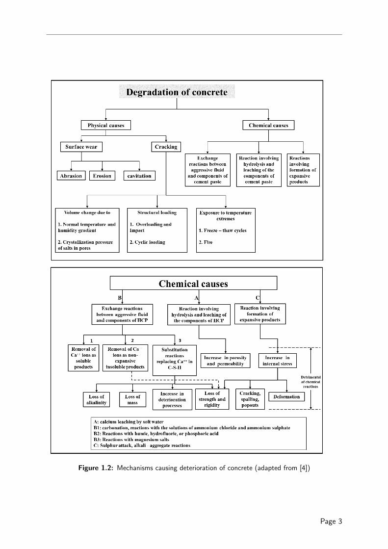
Figure 1.2: Mechanisms causing deterioration of concrete (adapted from [4])

Page 3

causing deterioration is a daunting task. Therefore reductionism2 is often applied while

studying deterioration of concrete both experimentally and numerically. Development of

experimental procedure for coupled processes is not always possible. However, numerical

models coupling different processes are relatively easy to develop. Moreover, many of the

deterioration mechanism are slow in nature (e.g. the progression of leaching under natural

condition is only upto few millimeters in hundred years! [17, 18]) and therefore often

the degradation processes are experimentally studied under accelerated conditions. Thus,

models form a crucial part in gerontology of concrete and can help to link the experimental

observations with reality.

Macro

Meso

Micro

Nano

Mortar, Concrete

Scale of interest

Cement paste

C-S-H

Concrete/mortar is treated as a homogenous material.

Morphological feature of concrete/mortar consists of cement paste, sand, aggregate and Interfacial Transition Zone (ITZ). Additionally thermal cracks formed during hydration and air voids can exist at this level.

Cement paste consists of amorphous C-S-H phase; crystalline hydration products such as portlandite, AFm phases (most common AFm phases are mono sulphate hydrates), AFt phases (most common AFt phase is ettringite), hydrogarnet; clinkers and capillary pores. The micro cracks formed during hydration can also exist at this level.

C-S-H phase consist of solid phase and gel porosity. There exist two types of C-S-H viz., low density C-S-H formed during earlier stage of hydration and high density C-S-H formed during later stage of hydration

Figure 1.3: Multi-scale representation of concrete

To better capture the behaviour at macroscopic scale due to ageing and its impact on

mechanical and transport properties, it is essential that the model accounts for changes

in morphology of concrete and able to simulate multi-physics processes. However, the

morphology of concrete presents a complex multi-scale nature as shown in Fig. 1.3 and

changes occur along each of this spatial scale during ageing. C-S-H forms the lowest

spatial scale (nano scale) of concrete. There is ample evidence to presume that C-S-H

exists in two different forms with two distinct volume fractions viz., low density C-S-H

(LD C-S-H) formed during early stage of hydration and (HD C-S-H) formed during later

stage of hydration in the pore spaces confined by existing C-S-H [15, 19–23]. The porosity

of the C-S-H matrix is commonly referred to as gel porosity. The gel pores can be further

2reductionism here refers to studying specific mechanism of deterioration and its influence on specificset of physical or chemical or mechanical property of concrete

Page 4

classified into interlayer pores, small gel pores (inter globule pores) and large gel mesopores

(inter LD pores) [22]. At micro scale concrete is represented by cement paste which

consists of C-S-H matrix, unhydrated clinker phases, crystalline hydration products such

as portlandite, AFm phases (most common AFm phases are mono sulphate hydrates),

AFt phases (most common AFt phase is ettringite), hydrogarnet; and capillary pores.

Additionally, at the micro scale, there might be micro cracks formed during hydration.

The meso scale refers to concrete/mortar that is composed of cement paste, aggregates

and interface between cement paste and aggregate the interface transition zone (ITZ). At

this level additionally large air voids and cracks formed during hydration can exist. Thus,

an accurate evaluation of concrete behavior due to aging requires the use of multi-scale

and multi-physics models.

The need for multi-scale models for concrete has been long realized in cement science.

Models have been proposed in order to provide the morphological description of concrete

at each of these scales during hydration (see for instance [24–29]). These models are

continuously being improved. Initiatives have also been undertaken to develop a multi-

scale framework to transfer parameters from lower scale to higher scales to obtain physical

and mechanical properties from these models (see for instance [29–33]).

There is still scope for improvement in these models in terms of providing reliable inputs

for these models (e.g. diffusivity of C-S-H). Secondly, there is a need to extend or develop

new multi-scale, multi-physics approaches for modeling ageing of concrete. The need for

such approaches is echoed in the concluding remarks of Ref. [34] by Prof. Klaas Van

Bruegel —

“Simulation models, based on sound material concepts, are of crucial importance for detecting

weak links in the quality chain. Furthermore, multi-scale and multidisciplinary models,

with a strong predictive power, will be essential for reliable service life predictions.”

Furthermore, development of multi-scale, multi-physics strategies would in turn require

development of models/tools to simulate changes due to aging in a wide range of length

scales (i.e., nano, micro and meso scale).

1.3 Research Objectives

Research objectives of this thesis are set based on the need to develop multi-scale and

multi-physics models in the field of gerontology of concrete. The specific objectives of this

thesis are defined as:

• To develop a numerical framework to simulate changes in morphology of cement

paste due to chemical degradation.

• Validate the numerical framework against several benchmark problems.

• To develop a more reliable approach to define transport parameters of C-S-H phase.

Page 5

• Demonstrating the usefulness of the developed framework by simulating calcium

leaching process.

1.4 Scope and limitations

The developed numerical framework considers only the reactive transport processes and its

application is limited to the ordinary Portland cement paste (micro scale of concrete) in

this study. However, the numerical framework developed in this study can be to meso and

macro length scales. Further, following modelling simplifications are made in this study

• Cement paste is considered to be fully saturated, which is not usually the case.

• Electro-kinetic effects on ion transport are not considered.

• Chemo-mechanical coupling (e.g., chemical shrinkage of C-S-H due to leaching) is

not considered.

• The influence of external temperature variations on chemical transport and reactions

is not considered.

1.5 Research strategy

A variety of approaches to model reactive transport processes at the pore-scale3 exist

(e.g. dissolution, precipitation or adsorption) and they involve different numerical schemes

such as finite volume method [35], pore network models [36, 37], smooth particle hydro-

dynamics [38, 39], hybrid approaches coupling different numerical methods[40–43] and

lattice Boltzmann methods [44–51]. In this study, lattice Boltzmann (LB) method has

been used as numerical framework. LB method presents a explicit algorithm with inherent

parallelism and simplistic handling of zero flux boundary condition through a bounce-back

rule4. Furthermore LB method also has certain advantages compared to other numerical

approaches commonly used such as —

• Geometry update (boundary tracking and remeshing) due to dissolution or precipi-

tation in traditional numerical methods (such as finite element and finite volume

methods) is time consuming.

• Algorithmic simplicity compared to the other methods

• Better stability and flexibility in time stepping compared to explicit finite difference

methods.

3pore-scale refers to the scale were pores and solids are explicitly resolved. Solids are considered to benon-diffusive at the pore-scale

4See chapter 2 for details

Page 6

• A three dimensional voxelized pore structure can be directly used for LBM whereas

for pore network method, an equivalent network representation of the pore structure

needs to be extracted.

Applicability of LBM has been successfully demonstrated for dissolution and precipitation

reactions [44–46, 49, 50]. This formulation has been further extended to incorporate

ion-exchange reactions [51]. However, in these approaches the heterogeneous reactions at

mineral grain boundary are conceptualized as as fluxes normal to the solid phase boundary,

which makes it difficult to separate the transport and reaction calculations and consequent

coupling of external geochemical codes. As a result, the applicability of LB method is yet

limited to fixed chemical systems. This shortcoming has also been highlighted in [35] —

“Lattice Boltzmann models are also efficient and scalable for flow and transport problems,

but they do not typically incorporate the wide range of geochemical reactions available in

many geochemical models.”

To eliminate this shortcoming, an alternate approach has been developed in this thesis

which enables coupling of LBM with external geochemical codes. Secondly, in case of

cement paste two scales co-exist. While C-S-H acts as a continuum media, crystalline

phases and clinker act as non diffusive phases and pore spaces are explicitly resolved

making a cement paste a multi-level porous media 5. Hence, a LBM for multi-level reactive

transport has also been developed in this thesis. The developed methods have been

implemented in a newly developed simulation tool called Yantra (in Sanskrit means a

tool or a device). The design philosophy and features of Yantra are detailed in Appendix

A. The developed framework has been applied to analyse the diffusivity of cement paste

microstructures and has been further adapted to simulate the calcium leaching of cement

paste. The diffusivity of C-S-H is determined by applying effective media theory. This

approach has been further extended to determine changes in diffusivity of C-S-H due to

leaching.

The input microstructures of the hydrated cement paste needed for these simulations are

obtained using the existing integrated kinetic models6. Several integrated kinetic models

exist, and have been reviewed in [28, 53]. These models simulate the microstructure

formation of cement paste during hydration using some basic inputs such as initial phase

composition of cement particles (clinkers), water to cement ratio, partial size distribution

or surface area of clinkers, and kinetic rate parameters which have been calibrated using

experimental data. These models can be divided into vector based models and lattice

5The term multi-level porous media is explained in Chapter 3.6The term integrated kinetic models has been coined by Van Breugel [52] to refer to hydration models

which describe the formation of inter particle contacts and their effect on the rate of reaction explicitly.These models, mostly computer-based simulation models, can be considered as operators, which generate,or have the potential to generate, micro-structural data in a direct way. Such an operator may consist ofa set of mathematical formulae or computational procedures for describing (changes in) the state of thespatial distribution of the anhydrous cement, the reaction products, the moisture state, and, if possible,the state of stresses which develop during hydration [28].

Page 7

based models [53].

In vector based models the cement particles are represented as spheres together with

co-ordinates of their centers. The hydration product are grown concentrically to the

cement particles. The dissolution of cement particles results in reduction in the radii of

clinker and growth of C-S-H layers results in increase of radii of C-S-H layers. The rate

of growth of C-S-H and reduction of clinkers is accounted for through a rate law. The

redistribution of product phases when growing product phases overlap is also accounted for

in such models. Phases such as calcium hydroxide grow spherically from initially defined

nuclei. The well-known vector models are HYMOSTRUC [52, 54] and µic [55, 56] (which

is a successor to Navi’s model [57, 58]).

In lattice based models a 3D cement paste microstructure is digitized on a uniform cubic

lattice and each volume element (voxel) is assigned certain material (e.g., water-filled

porosity, clinker phase, etc). The two well known lattice based models are CEMHYD3D

[59] and HydratiCA [60]. In CEMHYD3D the changes to the microstructure are simulated

through a large number of rules that are evaluated locally and depend on the materials

involved in the interaction, the temperature and, in some cases, global parameters describing

the microstructure such as the water/cement mass ratio or the volume fraction of a phase.

These rules are used to mimic the dissolution of solids, diffusion of dissolved species

according to a random walk algorithm, and nucleation and growth of hydration products

such as portlandite and C-S-H gel. HydratiCA is a reactive transport model based on

kinetic cellular automation and it directly simulates transport of ions, dissolution and

growth of mineral phases, complexation reactions at surface and nucleation of new phases.

In this thesis HYMOSTRUC and CEMHYD3D are used to obtain the input microstructures

of hydrated cement paste to cover both classes of cement paste microstructure models.

Both HYMOSTRUC and CEMHYD3D are available for download through following

links [61, 62] respectively, and almost all input parameters are self-explanatory in both

the models. The HYMOSTRUC model used in this thesis is more advanced than the

one available on-line and it includes also the nucleation and growth of portlandite. The

theoretical background for this version of HYMOSTRUC model can be found in reference

[63]

1.6 Summary of significant outcomes

• A new LB scheme (diffusion velocity lattice Boltzmann SRT scheme) has been

developed which allows for fixing the relaxation parameter to a value which best

suites the stability and accuracy with a flexibility of allowing for both variability of

time step and spatial heterogeneity of diffusion coefficients. This approach has been

further extended to simulate mass transport in a multi-level porous media.

Page 8

• A new approach has been developed to implement a generalized transport boundary

condition in LB scheme which is local and second order convergent.

• A new PID-controller (proportional, integral, differential) based adaptive relaxation

scheme has been developed to accelerate transient LB simulation.

• A new approach has been developed to treat heterogeneous reactions in LB reactive

transport schemes. This scheme has an ability to treat both homogeneous and

heterogeneous reactions in the same way thus replacing homogeneous and heteroge-

neous reactions with an equivalent total single source/sink term. This allows for the

coupling of LB schemes with the external geochemical codes.

• For the first time a successful coupling of LB schemes with the external geochemical

code PHREEQC [64] has been demonstrated.

• Extension of LB reactive transport schemes to multi-level porous media has been

demonstrated.

• A new two-scale model for C-S-H diffusivity based on effective media theory has

been developed. Using this model, developed LB framework for transport and

microstructures generated from integrated kinetic models viz., HYMOSTRUC and

CEMHYD3D the role of LD C-S-H porosity and HD C-S-H porosity has been

identified. It has been shown that for diffusion of tracers such as dissolved gases

(e.g. oxygen, helium) and HTO occurs only through LD C-S-H pores and HD C-S-H

pores do not contribute to transport. However, for electrical resistivity measurement

all gel pores contributes to the diffusion process. Due to this reason, the relative

diffusivity measured by electric resistivity techniques reported in literature is higher

than through diffusion experiments and electro-migration techniques.

• A simplified reactive transport model to simulate calcium leaching (from portlandite

and C-S-H phase) is developed. This model provides the same level of accuracy

as the detailed chemical reactions computation using geochemical thermodynamics.

The two scale diffusion model for C-S-H has been further extended to account for the

leaching. Using this approach for the first time (as per the best of author’s knowledge)

the reactive transport processes occurring in the microstructure of cement paste

due to calcium leaching (resulting in dissolution of portlandite and decalcification of

C-S-H) has been simulated.

1.7 Outline of the thesis

The outline of the thesis is schematically depicted in Fig. 1.4. The thesis is divided into

two parts. The numerical framework is presented in Part I. In chapter 2, a LB method is

Page 9

introduced and specific details for solute transport in a pore-scale system are introduced.

Two existing LB schemes viz., single relaxation method and two relaxation time method

are discussed. A newly developed diffusion velocity LB schemes is also detailed in this

chapter. Further, the existing approaches to implement generalized boundary conditions

for solute transport are compared and a new local approach to apply general boundary

conditions has been presented. In chapter 3, LB schemes to simulate solute transport in

multi-level porous media are presented. Two LB schemes to simulate solute transport

in multi-level porous media are discussed viz., diffusion velocity LB method and two

relaxation time LB method. In Chapter 4 LB schemes for simulating reactive transport

are presented. The LB scheme for simulating single mineral dissolution is first presented.

Next, the new LB scheme for multi-component reactive transport and coupling of LB

schemes with geochemical model PHREEQC is presented. Each of these chapters are

accompanied with series of benchmarks and examples to demonstrate the validity and

applicability of the developed schemes.

In Part II the developed framework is applied to obtain diffusivity from the microstructure,

generated from integrated kinetic models, and to simulate microstructural changes due

to calcium leaching in the cement paste. In Chapter 5 a critical appraisal of the existing

experimental data for cement paste is carried out. Further, a review of approaches

to estimate diffusivity and the models to obtain diffusivity from the microstructures

is presented. The approaches to estimate diffusivity are further compared with the

synthesised experimental data to reveal advantages and disadvantages of these approaches.

This chapter thus provides a state of the art and identifies the knowledge gaps in modeling

diffusivity of cement paste. In chapter 6, diffusivities are obtained from the microstructures

generated CEMHYD3D and HYMOSTRUC models. A new two-scale model for diffusivity

of C-S-H based on effective media theory has been presented. The diffusivity for a

wide range of experimental data is simulated from the microstructure generated from

integrated kinetic models and compared. Chapter 7 presents a review on the current

understanding on mechanisms of leaching, its impact on properties of cement paste and

both continuum and microstructural models developed for simulating leaching. Finally, in

Chapter 8, the developed numerical framework is applied to simulate leaching in cement

paste. A simplified approach to account for chemical reactions and the extension of the

two-scale diffusivity model for C-S-H, to account for leaching, is presented. Changes on

microstructure due to leaching are simulated on ordinary portland cement paste with two

different water-cement ratios. Chapter 9 presents a retrospection of the work carried out

in this thesis and the overall conclusions. It concludes with a brief discussion on a way

forward to extend the present work to address more complex issues in modeling of aging

concrete.

Page 10

Chap

ter

4:

latt

ice

Bolt

zman

n m

etho

d f

or

reac

tiv

e tr

ansp

ort

Chap

ter

3:

Lat

tice

Bolt

zman

n m

etho

d

for

solu

te t

ran

sport

in

mult

ilev

el

po

rou

s m

edia

Chap

ter

2:

Lat

tice

Bolt

zman

n

met

hod f

or

solu

te t

ran

spo

rt a

t

po

re s

cale

Ch

apte

r 1:

Intr

odu

ctio

n

Part

I:

Nu

meri

cal

fram

ewo

rk

Ch

apte

r 9:

Ret

rosp

ecti

on

, C

on

clu

sio

ns

and W

ay f

orw

ard

Pa

rt I

I: A

pp

lica

tio

ns

to

cem

en

t b

ase

d m

ate

rials

Ch

apte

r 5

: C

riti

cal

app

rais

al o

f ex

per

imen

tal

dat

a an

d m

odel

s fo

r

dif

fusi

vit

y o

f ce

men

t

pas

te

Chap

ter

6:

Det

erm

inat

ion

of

effe

ctiv

e dif

fusi

vit

y f

rom

inte

gra

ted

kin

etic

mo

del

s: r

ole

of

morp

ho

log

y

Ch

apte

r 8

: M

od

elli

ng

chan

ges

in m

icro

stru

cture

of

cem

ent

pas

te u

nd

er

calc

ium

lea

chin

g

Lit

erat

ure

rev

iew

rel

evan

t

to m

od

elin

g w

ork

per

form

ed i

n t

his

thes

is

Chap

ter

7:

Lea

chin

g o

f

cem

ent

pas

te:

mec

han

ism

s,

infl

uen

ce o

n p

roper

ties

and

exis

ting

mo

del

lin

g

appro

aches

Figure 1.4: Oultine of the thesis

Page 11

Part I: Numerical model development

Page 13

CHAPTER 2

Lattice Boltzmann method for solute transport at pore-scale

The pore-scale in this thesis refers to the explicit representation of the solids and pores

spaces as shown in Fig. 2.1. For the definition of the pore-scale used in this thesis solids

are considered non-diffusive. Thus diffusion occurs only through pore fluid.

Figure 2.1: A representation of pore-scale system

In this chapter the lattice Boltzmann (LB) method is introduced to solve the governing

equation (advection-diffusion equation) for solute transport at pore-scale. The details on

governing equation are presented in Chapter 2.1. The LB methods to solve the governing

equation are described in section 2.2. In this chapter first the general idea of LB methods is

introduced and two existing LB formulations single relaxation time (SRT) LB method and

two relaxation time (TRT) lattice Boltzmann method are presented. SRT LB is the most

Page 15

simple LB formulation however it has certain disadvantages such as restrictive variability

of relaxation parameter which in turn results in restrictive variability of diffusion coefficient

and slower convergence to steady state. To eliminate this shortcoming a new SRT diffusion

velocity LB formulation is developed. In the final part of this chapter approaches to

implement initial and Boundary conditions in LB method are presented. A particular focus

is laid in discussing and comparing different approaches to implement generalized boundary

conditions for advection-diffusion equation. Also, a new local approach to implement

generalized boundary condition for LB schemes with orthogonal lattices is proposed which

is better in terms of accuracy and convergence compared to existing approaches. Finally,

benchmarks and examples to highlight advantages of a SRT diffusion velocity LB method

over SRT scheme are presented in section 2.3.

2.1 Governing equations

The solute transport at the pore-scale can be described using advection-diffusion equation.

∂C

∂t= −~∇ · ~J (2.1)

~J = −D0~∇C + ~uC

where C is the concentration [NL−3], ~u is the pore velocity vector [LT−1], ~J is the flux

vector and D0 is the molecular diffusion coefficient of the solute in pore water [L2T−1].

As the solid phase is non-diffusive, a zero flux boundary condition is to be imposed at the

surface of the solids~J · n |Γs= 0 (2.2)

n is the unit normal vector and Γs represents the boundary of the non diffusive solid phase.

The domain boundary conditions in general can be written as

A1C + A2n~∇C = A3 (2.3)

A1, A2 and A3 are constants. The special forms of the boundary condition can be deduced

form Eq. (2.3) using different values of A1, A2 and A3 as given below

Dirichlet boundary: A1 = 1, A2 = 0

Neumann boundary: A1 = 0, A2 = 1

Cauchy boundary: A1 = ~ub, A2 = −D0 A3 = Cb~ub

Cb and ~ub are concentration and pore velocity at boundary.

Page 16

2.2 Lattice Boltzmann method

Lattice Boltzmann (LB) methods solves a discrete form of continuous Boltzmann equation.

The Boltzmann transport equation describes the evolution of the density of particles

f(~r, t, ~e) [N1L−3] at time t [T], at the point with position vector ~r [L], having same velocity

~e [L−1T]. Alternatively f(x, t, ~e) can also be thought of as the probability of finding a

particle with velocity ~e near the point with position vector ~r at time t and hence it is also

referred to as single particle distribution function. In this thesis f(~r, t, ~e) is shortly referred

to as distribution function. The Boltzmann transport equation in absence of external force

is given as∂f

∂t+ ~e · ~∇f = Ω (2.4)

Ω is the collision operator 1. The left hand side of Eq. (2.4) is referred to as streaming

operator and it relates to streaming of f from one point to another. This operator can be

physically viewed as streaming of f from ~r to ~r + ~e∆t in time interval ∆t in case there is

no collision i.e. right hand side of Eq. (2.4) is zero.

The discretization of the Boltzmann equation is carried out in space,time and velocity in

order to obtain LB equation. The Boltzmann equation discretized with respect to velocity

space can be written as

∂fi∂t

+ ~ei · ~∇fi = Ωi, i = 1, 2, ..., q (2.5)

~ei refers to discrete velocity vector. The velocity space in LB method is discretized in

a regular lattice arrangement (as discussed later). Therefore in LB method, streaming

occurs along the regular lattice. Hence the name “Lattice Boltzmann” method. Further

discretization of Eq. (2.5) with respect to space and time gives (for details see Appendix

B)

fi(~r + ~ei∆t, t+ ∆t) = fi(~r, t) + ∆tΩi(~r, t) (2.6)

Eq. (2.6) is the lattice Boltzmann equation. The collision term in its general form for LB

method can be written as

Ωi = −Λij

(fj − f eqj

)(2.7)

Λij is the matrix of the adjustable relaxation parameters, and f eq is the single particle

distribution function at equilibrium [N1L−3] which is shortly referred to as equilibrium

distribution function in this Thesis. The choice of the equilibrium distribution function

and the type of lattice depends on the type of equation (physics) to be solved.

The distribution function and equilibrium function additionally need to satisfy a certain

set of conditions in order to conserve certain physical quantities. For advection-diffusion

1In the original Boltzmann equation the collision operator is derived by considering interaction betweentwo particles during collision.

Page 17

only the conservation of mass is required during the collision step. This can be achieved

by enforcing following condition ∑i

fi =∑i

f eqi = C (2.8)

In case of Navier-Stokes equation additionally conservation of momentum is needed during

the collision step which can be achieved by following condition∑i

fi~ei =∑i

f eqi ~ei = ρf~u (2.9)

ρf being the density of the fluid [ML−3]. If energy has to be conserved in lattice Boltzmann

method following condition has to be met,∑i

fi(~ei − ~u) · (~ei − ~u) =∑i

f eqi (~ei − ~u) · (~ei − ~u) = 2ρfE (2.10)

where E is the energy [ML2T−2]. It can be shown that the solution of lattice Boltzmann

equation (Eq. (2.6)) leads to solution of advection-diffusion equation (Eq. (2.1)) at the

asymptotic limits through a multi-scale Chapman-Enskog expansion which is explained in

detail in later part of this chapter.

Remark 2.2.1 (History of lattice Boltzmann method) The predecessor to the lattice

Boltzmann method are lattice gas automata wherein the fluid is represented as a set of

particles moving on a defined lattice geometry and follows a simple set of collision rules. The

break through in field of lattice gas automata to simulate fluid was achieved when Frisch et al.

[65] demonstrated that particles moving on a defined lattice with a simple set of collision

rules are able to mimic fluid flow. Soon after the drawbacks of lattice gas automata were

realized such as large statistical noise, limited range of physical parameters, non-Galilean

invariance, and implementation difficulty in three dimensions. To circumvent this drawback

the lattice Boltzmann equation was introduced by Higuera and Jimenez [66]. In the original

lattice Boltzmann method the equilibrium distribution functions and the relaxation matrix

were derived from the underlying lattice gas automata models. Higuera et al. [67] further

showed that the lattice Boltzmann equations can be derived independently of underlying

lattice gas automata. Later on Qian et al. [68] suggested that the collision term can be

replaced by a a linear term with a single relaxation parameter similar to one proposed by

Bhatnagar et al. [69]. This is still the most popular LB scheme due to its algorithmic

simplicity. However it has certain drawbacks (discussed later in this section). About a

decade later, D’Humieres et al. [70] presented a theoretical framework for obtaining the

matrix of relaxation parameters. They introduced this framework as Multi Relaxation Time

(MRT) lattice Boltzmann method. The idea behind the MRT scheme is to relax the moments

Page 18

of distribution function rather than the distribution function as moments are related to

physical quantities. The distribution function are transformed to moment space using the

transformation matrix. The matrix of relaxation parameters is given by M−1 · S ·M . Here

M is the transformation matrix which maps the distribution function to moment space and

S is the matrix representing the relaxation parameter for the moments.

2.2.1 Equilibrium distribution function

The equilibrium distribution function (EDF) is based on the Maxwell-Boltzmann distribu-

tion (see Appendix C for detail discussion). Linear part of Maxwell-Boltzmann distribution

is enough for advection-diffusion equation, as it do not contain the second order terms of

pore velocity [71].

f eqi = wiC

(1 +

~ei · ~ue2s

)i > 0

= C −i=q∑i=1

f eqi i = 0

(2.11)

wi are the lattice weights and es is the pseudo lattice speed of sound. The values of wi

and es depend on type of lattice. Alternatively the second order EDF (quadratic with

respect to velocity terms) which is used for Navier-Stokes equation has also been used for

advection-diffusion equation. It will be shown in later part of the discussion that second

order EDF alongwith higher order lattice can recover advection-diffusion equation without

any error terms upto second order during Chapman-Enskog expansion.

f eqi = wiC

(1 +

~ei · ~ue2s

+~ei~ei : ~u~u

2e4s

− ~u · ~u2e2

s

)i > 0

= C −i=q∑i=1

fi i = 0

(2.12)

2.2.2 Lattice structures

A lattice structure with q lattice directions in d dimensions is commonly referred to as

”DdQq lattice” as suggested by Qian et al. [68]. The lattice structure defines the path for

streaming of distribution function from current cell to the neighbouring cell. The number

of neighbours in the lattice structure depends on the quantities to be conserved. For a

regular lattice a unique set of velocity moments exist only up to certain order. This is

referred to as isotropy of the lattice. The order of the moment upto which unique values

exists are referred to as order of isotropy of the lattice. Furthermore, the lattices with

more directions will have higher order of isotropy. For mass conservation lattices should

be at least second order isotropic. For mass and momentum conservation lattices with at

Page 19

least fourth order isotropy are required.

For advection-diffusion as only mass conservation is needed, the lattices should be at

least second order isotropic. The formal definition of the second order isotropic lattice

structures can be laid as, their exists wi, es and velocity vectors ~ei such that following

conditions are satisfied.∑i

wi = 1,∑i

wieiα = 0,∑i

wieiαeiβ = e2sδαβ (2.13)

Eq. 2.13 is written in indicial notations and α,β refers to spatial directions. In this thesis

indicial and vector notations are used interchangeably due to complexity of mathematical

expressions. The notations are kept in vector form where ever possible.

These criteria are easily met by lattices which are pointing toward its immediate neighbour.

In three-dimensions immediate neighbour refers to cells sharing faces, edge or corners.

For these lattices weights can be divided into three types: w0 for rest or zero velocity, ws

for lattice velocity in orthogonal direction and wl for lattice velocity in non orthogonal

direction. The commonly used lattices with immediate neighbours are given below

D2Q5

e2s = e/3 (2.14)

w0 = 2/6 ws = 1/6

~e0 = (0, 0)

~e1 = (e, 0) ~e2 = (0, e)

~e3 = (−e, 0) ~e4 = (0,−e)

D3Q7

e2s = e/3.5 (2.15)

w0 = 1/7 ws = 1/7

~e0 = (0, 0, 0)

~e1 = (e, 0, 0) ~e2 = (0, e, 0) ~e3 = (0, 0, e)

~e4 = (−e, 0, 0) ~e5 = (0,−e, 0) ~e6 = (0, 0,−e)

Page 20

D2Q9

e2s = e/3 (2.16)

w0 = 4/9 ws = 1/9 wl = 1/36

~e0 = (0, 0)

~e1 = (e, 0) ~e2 = (0, e) ~e3 = (−e, 0) ~e4 = (0,−e)

~e5 = (e, e) ~e6 = (−e, e) ~e7 = (−e,−e) ~e8 = (−e, e)

D3Q15

e2s = e/3 (2.17)

w0 = 2/9 ws = 1/9 wl = 1/72

~e0 = (0, 0, 0)

~e1 = (e, 0, 0) ~e2 = (0, e, 0) ~e3 = (0, 0, e)

~e4 = (−e, 0, 0) ~e5 = (0,−e, 0) ~e6 = (0, 0,−e)

~e7 = (−e,−e,−e) ~e8 = (−e,−e, e) ~e9 = (−e, e,−e)

~e10 = (−e, e, e) ~e11 = (e, e, e) ~e12 = (e, e,−e)

~e13 = (e,−e, e) ~e14 = (e,−e,−e)

D3Q19

e2s = e/3 (2.18)

w0 = 1/3 ws = 1/18 wl = 1/36

~e0 = (0, 0, 0)

~e1 = (e, 0, 0) ~e2 = (0, e, 0) ~e3 = (0, 0, e)

~e4 = (−e, 0, 0) ~e5 = (0,−e, 0) ~e6 = (0, 0,−e)

~e7 = (−e, 0, e) ~e8 = (0,−e,−e) ~e9 = (0,−e, e)

~e10 = (−e,−e, 0) ~e11 = (−e, e, 0) ~e12 = (−e, 0,−e)

~e13 = (e, e, 0) ~e14 = (e,−e, 0) ~e15 = (e, 0, e)

~e16 = (e, 0,−e) ~e17 = (0, e, e) ~e18 = (0, e,−e)

where e is ∆r/∆t. ∆r being distance between two lattice nodes [L] and ∆t is the discrete

time step [T].

Page 21

Table 2.1: Velocity moments of different lattices upto 4th order

moments of lattice weights D2Q5, D3Q7 D2Q9, D3Q15, D3Q19∑wi 1 1∑wieiα 0 0∑wieiαeiβ e2

sδαβ e2sδαβ∑

wieiαeiβeiγ 0 0∑wieiαeiβeiγeiδ e2

sδαβγδ e4s∆

4αβγδ

Remark 2.2.2 (Isotropy of velocity moments) Chen et al. [72] has provided the for-

mal definition of isotropy of velocity moments. A lattice is considered nth order isotropic if

following conditions are satsified:

∑i

eiα1eiα2 · · · eiαn = ens∆nα1α2···αn n = 2, 4, 6, · · ·

∑i

eiα1eiα2 · · · eiαn = 0 n = 1, 3, 5, · · ·

Here ∆nα1,α2,··· ,αn is the isotropic delta function. It is defined as the sum of n/2 products

of Kronecker delta functions δα1,α2 · · · δαn−1,αn in over all distinctive permutations of its

sub-indices. There are (n− 1)!!(≡ (n− 1) · (n− 3) · · · 3 · 1) distinctive terms in ∆nα1α2···αn.

For instance

∆2α1α2 = δα1α2

and

∆4α1α2α3α4 = δα1α2δα3α4 + δα1α3δα2α4 + δα1α4δα2α3

Table 2.1 shows the velocity moments for various lattices listed above upto 4th order. It

can be observed that orthogonal lattices only possesses 2nd order isotropy according to the

definition provided above and hence they fail to recover Naiver-Stokes equation [65].

2.2.3 Single relaxation time lattice Boltzmann method

In single relaxation time (SRT) LB method the matrix of the adjustable relaxation

parameters is replaced by the single relaxation parameter (τ). The resulting collision term

is the one proposed by Bhatnagar et al. [69] and it is therefore also referred to as BGK

collision term (ΩBGK). The SRT LB equation is given as

fi(~r + ~ei∆t, t+ ∆t) = fi(~r, t) + ∆tΩBGKi (~r, t) (2.19)

ΩBGKi (~r, t) = −1

τ(fi(~r, t)− f eqi (~r, t))

It can be shown using multi-scale Chapman-Enskog expansion that at asymptotic limit

Eq.(2.19) gives an advection-diffusion equation. The first step in Chapman-Enskog

Page 22

expansion is to expand left hand side of Eq. (2.19) using Taylor series expansion. Then the

space and time derivatives are expanded with respect to a small perturbation parameter ε.

The time derivative is expanded as

∂

∂t= ε

∂

∂t1+ ε2 ∂

∂t2+O(ε3) (2.20)

and space derivative is expanded as

~∇ = ε~∇∗ +O(ε2) (2.21)

The distribution function is likewise expanded starting from zeroth order.

fi = f(0)i + εf

(1)i + ε2f

(2)i +O(ε3) (2.22)

The space and time derivatives are then replaced using Eq. (2.21) and Eq. (2.20) and

distribution function is replaced using Eq. (2.22). The details of the derivation of

Chapman-Enskog expansion upto this step are presented in Appendix (D). Eq. (2.20)

implies that two time scales exist viz., advective time scale (t1) and diffusive time scale

(t2). The advective component is mapped as t1 → εt and diffusive component is mapped

as t2 → ε2t. The distribution function is thus mapped from fi(r, t) to fi(r∗, t1, t2). The

Chapman-Enskog expansion thus allows to separate the phenomena occurring at different

scales and by comparing the terms with same order of ε conservation laws and physical

phenomena at each scale can be discussed separately. For SRT LB equation applying

Chapman-Enskog expansion and comparing the terms with same order of ε leads to

following relations

O(ε0) :− ∆t

τ

(f

(0)i − f

eqi

)= 0 (2.23)

O(ε1) :

[∂

∂t1+ ~ei · ~∇∗

]f

(0)i = −1

τf

(1)i (2.24)

O(ε2) :

[∂

∂t2+

∆t

2

∂2

∂t21+ ∆t

∂

∂t1~ei · ~∇∗ +

∆t

2~ei~ei : ~∇∗~∇∗

]f

(0)i +

[∂

∂t1+ ~ei · ~∇∗

]f

(1)i

= −1

τf

(2)i (2.25)

from O(ε0) it can be deduced that f(0)i = f eqi and applying condition given by Eq. (2.8)∑

i

fi =∑i

f(0)i =

∑i

f eqi = C and∑i

f(1)i =

∑i

f(2)i = 0 (2.26)

Page 23

Taking zeroth order moment over O(ε1) equation and using Eq. (2.26) we get

∑i

[∂

∂t1+ ~ei · ~∇∗

]f

(0)i = 0 (2.27)

Substituting O(ε1) in O(ε2) equation we can rewrite O(ε2) in terms of f(0)i .[

∂

∂t2+

(∆t

2− τ)∂2

∂t21+ (∆t− 2τ)

∂

∂t1~ei · ~∇∗ +

(∆t

2− τ)~ei~ei : ~∇∗~∇∗

]f

(0)i = −1

τf

(2)i

(2.28)

Taking zeroth order moment over Eq. (2.28)

∂∑

i f(0)i

∂t2+

(∆t

2− τ)∂2∑

i f(0)i

∂t21+(∆t− 2τ)

∂

∂t1~∇∗·∑i

f(0)i ~ei+

(∆t

2− τ)~∇∗2

∑i

f(0)i ~ei~ei = 0

(2.29)

from Eq. (2.27)∂2

∑i f

(0)i

∂t21can be rewritten as

∂2∑

i f(0)i

∂t21= −~∇∗ ·

∑i

f(0)i ~ei (2.30)

substituting (2.30) in (2.29)

∂∑

i feqi

∂t2+

(∆t

2− τ)

∂

∂t1~∇∗ ·

∑i

f eqi ~ei +

(∆t

2− τ)~∇∗2

∑i

f eqi ~ei · ~ei = 0 (2.31)

substituting the relevant moments of f eqi in Eq. (2.31) advection diffusion equation can be

recovered. Table 2.2 shows the moments of f eqi for different lattice structures and choice

of EDF. The first LHS term of Eq. (2.31) irrespective of lattice structure or EDF can be

written as∂∑

i feqi

∂t2=∂C

∂t2(2.32)

using Eq.(2.20) Eq. (2.27) and (2.21) in Eq. (2.32)

∂∑

i feqi

∂t2=

1

ε2

(∂C

∂t+ ~∇·~uC

)(2.33)

The second LHS term of Eq. (2.31) irrespective of lattice structure and EDF can be

written as (∆t

2− τ)

∂

∂t1~∇∗ ·

∑i

f eqi ~ei =

(∆t

2− τ)~∇∗ ·

[~u∂C

∂t1+ C

∂~u

∂t1

](2.34)

Page 24

Table 2.2: Moments up to second orders of equilibrium distribution functions for different lattices

Lattices moments Linear QuadraticD2Q5,D3Q7

∑f eqi C C∑f eqi eiα Cuα Cuα∑f eqi eiαeiβ Ce2

sδαβ C[(e2s −

uγuγ2

)δαβ +

uγuδδαβγδ2e2s

]D2Q9,D3Q15,D3Q19

∑f eqi C C∑f eqi eiα Cuα Cuα∑f eqi eiαeiβ Ce2

sδαβ C [e2Sδαβ + uαuβ]

Considering no rapid time variation of flows ∂~u∂t1

= 0, assuming flow and using Eq. (2.27)(∆t

2− τ)

∂

∂t1~∇∗ ·

∑i

f eqi ~ei = −(

∆t

2− τ)~∇∗~u~u~∇∗C (2.35)

Assuming flow to be incompressible ∇ · ~u = 0 and using Eq. (2.21)(∆t

2− τ)

∂

∂t1~∇∗ ·

∑i

f eqi ~ei = − 1

ε2

(∆t

2− τ)~u · ~u~∇2C (2.36)

The third LHS term of Eq. (2.31) depends on type of EDF and lattice structure. For a

linear EDF irrespective of the lattice structure using (2.21) the third LHS term can be

rewritten as (∆t

2− τ)~∇∗2

∑i

f eqi ~ei · ~ei =1

ε2e2s

(∆t

2− τ)~∇2C (2.37)

For orthogonal lattice structures with quadratic EDF the third LHS term of Eq. (2.31)

becomes(∆t

2− τ)~∇∗2

∑i

f eqi ~ei · ~ei =1

ε2

[(e2s −

uγuγ2

)δαβ +

uγuδδαβγδ2e2

s

](∆t

2− τ)∇αβC

(2.38)

for higher order lattice structures with quadratic EDF the third LHS term of Eq. (2.31) is

then written as(∆t

2− τ)~∇∗2

∑i

f eqi ~ei · ~ei =1

ε2

(e2s + ~u · ~u

)(∆t

2− τ)~∇2C (2.39)

Finally the advection-diffusion equation can be recovered by re substituting these terms

back in Eq. (2.31).

• All lattice structures with linear EDF

∂C

∂t+ ~∇C · ~u =

(τ − ∆t

2

)(e2s − ~u · ~u

)~∇2C (2.40)

Page 25

• Orthogonal lattice structures with quadratic EDF

∂C

∂t+∇αCuα =

[e2sδαβ +

(uγuδδαβγδ

2e2s

− uγuγ2

δαβ − uαuβ)](

τ − ∆t

2

)∇αβC

(2.41)

• Higher order lattice structures with quadratic EDF

∂C

∂t+ ~∇C · ~u = e2

s

(τ − ∆t

2

)~∇2C (2.42)

Comparing equations Eq. (2.40), Eq. (2.41) and Eq. (2.42) the diffusion coefficient is

obtained as

D0 = e2s

(τ − ∆t

2

)(2.43)

It can be observed from Eq. (2.40), Eq. (2.41) and Eq. (2.42) that only higher order

lattice structures with quadratic EDF recover the advection-diffusion equation without

any error terms. This result has also been confirmed by other researchers [73, 74]. It can

be further deduced that for the linear EDF and orthogonal lattice structure with quadratic

EDF the error term vanishes under assumption ~u·~ue2s≈ 0. Flekkoy [71] was the first to

use linear EDF to recover advection diffusion equation. He argued that ~u is small in the

incompressibility limit 2 and the term ~u · ~u represents only 1% of correction and hence

these terms can be effectively neglected.

Remark 2.2.3 (removing error terms in case of linear EDF) The error terms aris-

ing while recovering the advection-diffusion equation using linear EDF can be corrected by

introducing a forcing term of form wi~ei · ~F [74, 75]. This forcing term is added to collision

term. During Chapman-Enskog expansion the the forcing term is expanded as ~F = ε~F(1)

and hence Eq. (2.24) can be rewritten as[∂

∂t1+ ~ei · ~∇∗

]f

(0)i = −1

τf

(1)i + wi~ei · ~F

(1)

Correspondingly the O(ε2) in terms of f(0)i can be written as

[∂

∂t2+

(∆t

2− τ)∂2

∂t21+ (∆t− 2τ)

∂

∂t1~ei · ~∇∗ +

(∆t

2− τ)~ei~ei : ~∇∗~∇∗

]f

(0)i +

τ

[∂

∂t1+ ~ei · ~∇∗

]wi~ei · ~F

(1)= −1

τf

(2)i

2Incompressibility refers to the assumption that if the flow remains within a Mach number limit(normally less than 0.3) the fluid flow is treated as incompressible flow

Page 26

Taking the zeroth moment over above equation we get

[∂

∂t2+

(∆t

2− τ)∂2

∂t21+ (∆t− 2τ)

∂

∂t1~ei · ~∇∗ +

(∆t

2− τ)~ei~ei : ~∇∗~∇∗

]∑i

f(0)i +

τe2s~∇∗ · ~F(1)

= 0

Further using Eq. (2.24), the term ∂2

∂t21

∑i fi can be replaced by − ∂

∂t1~ei · ~∇∗

∑i fi resulting

in [∂

∂t2

(∆t

2− τ)

∂

∂t1~ei · ~∇∗ +

(∆t

2− τ)~ei~ei : ~∇∗~∇∗

]∑i

f(0)i + τe2

s~∇∗ · ~F(1)

= 0

Further continuing the derivation for recovering the advection-diffusion equation from above

equation it can be observed that in order to recover the advection-diffusion equation without

error term following condition should be satisfied(τ − ∆t

2

)∂C~u

∂t− τe2

s~F = 0

which leads to

~F =1

e2s

(1− ∆t

2τ

)∂C~u

∂t=

1

e2s

(1− ∆t

2τ

)[C∂~u

∂t+ ~u

∂C

∂t

]=

1

e2s

(1− ∆t

2τ

)[C(t+∆t)~u

(t+∆t) − ~u(t)

∆t+ ~u(t+∆t)C

(t+∆t) − C(t)

∆t

]

In case the rest velocity is present in the lattice structure ∂C∂t can be expressed in terms of

fneq0 = f0 − feq0 using Eq. (2.24) as

∂C

∂t= − 1

τw0fneq0

Remark 2.2.4 (Implementation) LB methods has a Lagrangian nature. Hence conven-

tionally, LB methods is implemented in two steps: collide and stream. In collide step the

collision term is evaluated and in place modification of distribution function is made. In

the stream step the distribution functions are advected to the neighbouring node based on a

given lattice structure. The collide-stream algorithm for the two dimensional SRT lattice

Boltzmann method is shown in Algorithm 2.1. As shown in the pseudo code during streaming

step two copies of distribution function are required. This can be avoided by using a swap

algorithm [76]. Collide-stream algorithm needs at least two passes over the memory which is

memory band width intensive. To circumvent this several fused algorithms (applying collide

and stream in one go) have been proposed (for details of fused algorithms and comparison

Page 27

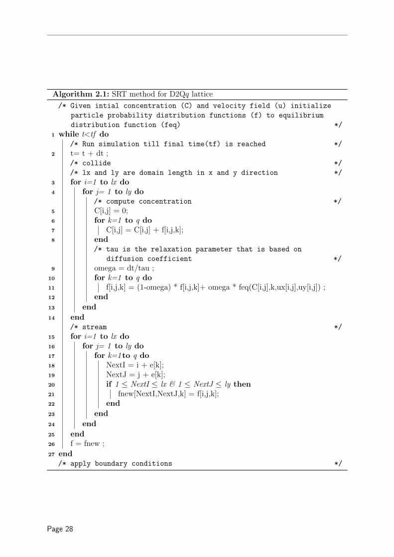
Algorithm 2.1: SRT method for D2Qq lattice

/* Given intial concentration (C) and velocity field (u) initialize

particle probability distribution functions (f) to equilibrium

distribution function (feq) */

1 while t<tf do/* Run simulation till final time(tf) is reached */

2 t= t + dt ;/* collide */

/* lx and ly are domain length in x and y direction */

3 for i=1 to lx do4 for j= 1 to ly do

/* compute concentration */

5 C[i,j] = 0;6 for k=1 to q do7 C[i,j] = C[i,j] + f[i,j,k];8 end

/* tau is the relaxation parameter that is based on

diffusion coefficient */

9 omega = dt/tau ;10 for k=1 to q do11 f[i,j,k] = (1-omega) * f[i,j,k]+ omega * feq(C[i,j],k,ux[i,j],uy[i,j]) ;12 end

13 end

14 end/* stream */

15 for i=1 to lx do16 for j= 1 to ly do17 for k=1 to q do18 NextI = i + e[k];19 NextJ = j + e[k];20 if 1 ≤ NextI ≤ lx & 1 ≤ NextJ ≤ ly then21 fnew[NextI,NextJ,k] = f[i,j,k];22 end

23 end

24 end

25 end26 f = fnew ;

27 end/* apply boundary conditions */

Page 28

between different algorithms refer [77, 78]).

Remark 2.2.5 (D2Q5 vs D2Q9) Suga [79] carried out stability analysis for D2Q5 and

D2Q9 lattices with linear EDF. His conclusions showed that the stability conditions of the

D2Q9 are more restrictive than those of D2Q5. Further, his numerical experiments suggest

that for a grid Peclet number greater than 10, D2Q9 gives more accurate results than D2Q5

lattice for a given Courant number. However in his study the e2s for D2Q5 and D2Q9 lattices

are different viz. 1/2 and 1/3 respectively. Hence for a given Courant number D2Q5 and

D2Q9 lattices yields different relaxation parameters. It has been shown by Servan-Camas

[74] that the accuracy of SRT scheme is dependent on relaxation parameter. Servan-Camas

[74] further showed that for a grid Peclet number 40, D2Q5 lattice with corrected linear

EDF ( see Remark 2.2.3) shows good match with analytical method. Moreover, D2Q5 is

more efficient than D2Q9 lattice both in terms of both memory and computation. Hence

D2Q5 lattice is a good choice for pore scale solute transport and for higher Peclet number

the correction to linear EDF should be taken into account.

2.2.4 Two relaxation time lattice Boltzmann method

In two relaxation time (TRT) lattice Boltzmann method the symmetric and anti-symmetric

parts of the particle distribution function are relaxed separately using two different

relaxation parameters. The symmetric (f+)and anti-symmetric parts (f−) of the particle

distribution functions are defined as

f+i =

fi + f−i2

& f−i =fi − f−i

2(2.44)

where fi and f−i refers to distribution functions corresponding to lattice velocity ~ei and

~e−i respectively; ~ei = −~e−i. The above definition of symmetric and anti-symmetric part

naturally imposes a condition that all the even moments of anti-symmetric part and odd

moments of symmetric parts are zero. The two relaxation time lattice Boltzmann equation

is written as follows [73]

fi(~r + ~ei∆t, t+ ∆t) = fi(~r, t) + ∆tΩTRTi (~r, t) (2.45)

ΩTRTi (~r, t) = − 1

τ+

(f+i (~r, t)− f eq+i (~r, t)

)− 1

τ−

(f−i (~r, t)− f eq−i (~r, t)

)(2.46)

Here, τ+ and τ− are relaxation parameters for the symmetric part and anti-symmetric part

respectively. Applying Chapman-Enskog expansion to TRT scheme given by Eq. (2.45)

Page 29

and separating the terms with same order of ε we get

O(ε0) :− ∆t

τ+

(f

+(0)i − f eq+i

)− ∆t

τ−

(f−(0)i − f eq−i

)= 0 (2.47)

O(ε1) :

[∂

∂t1+ ~ei · ~∇∗

]f

(0)i = − 1

τ+

f+(1)i − 1

τ−f−(1)i (2.48)

O(ε2) :

[∂

∂t2+

∆t

2

∂2

∂t21+ ∆t

∂

∂t1~ei · ~∇∗ +

∆t

2~ei~ei : ~∇∗~∇∗

]f

(0)i +

[∂

∂t1+ ~ei · ~∇∗

]f

(1)i

= − 1

τ+

f+(2)i − 1

τ−f−(2)i (2.49)

from O(ε0) terms under the condition imposed by Eq. (2.8) we get∑i

fi =∑i

f(0)i =

∑i

f+(0)i = C and∑

i

f(1)i =

∑i

f(2)i = · · · = 0 and∑

i

f+(1)i =

∑i

f+(2)i = · · · = 0 (2.50)

Taking zeroth moment over O(ε1) terms Eq. (2.27) can be recovered. Finally taking zeroth

moment over O(ε2) terms

∑i

[∂

∂t2+

∆t

2

∂2

∂t21+ ∆t

∂

∂t1~ei · ~∇∗ +

∆t

2~ei~ei : ~∇∗~∇∗

]f

(0)i + ~∇∗ ·

∑i

f(1)i ~ei = 0 (2.51)

using Eq. (2.27)

∂2∑

i f(0)i

∂t21= − ∂

∂t1~ei · ~∇∗

∑i

f(0)i (2.52)

Taking first moment over O(ε1) terms it can be shown that

~∇∗ ·∑i

f(1)i ~ei = ~∇∗ ·

∑i

f−(1)i ~ei = −τ−

∑i

[∂

∂t1~ei · ~∇+ ~ei~ei : ~∇∗~∇∗

]f

(0)i (2.53)

substituting Eq. (2.52) and Eq. (2.53) in Eq. (2.51)

∂∑

i feqi

∂t2+

(∆t

2− τ−

)∂

∂t1~∇∗ ·

∑i

f eqi ~ei +

(∆t

2− τ−

)~∇∗2

∑i

f eqi ~ei · ~ei = 0 (2.54)

Eq. (2.54) is same as Eq. (2.31) with τ now replaced by τ−. Following the further

derivation as shown in Section 2.2.3 it can be shown that similar to SRT scheme the

scheme advection-diffusion equation can be recovered at asymptotic limits.

Page 30

• All lattice structures with linear EDF

∂C

∂t+ ~∇C · ~u =

(τ− −

∆t

2

)(e2s − ~u · ~u

)~∇2C (2.55)

• Orthogonal lattice structures with quadratic EDF

∂C

∂t+∇αCuβ =

[e2sδαβ +

(uγuδδαβγδ

2e2s

− uγuγ2

δαβ − uαuβ)](

τ− −∆t

2

)∇αβC

(2.56)

• Higher order lattice structures with quadratic EDF

∂C

∂t+ ~∇C · ~u = e2

s

(τ− −

∆t

2

)~∇2C (2.57)

and the diffusion coefficient is given as

D0 = e2s

(τ− −

∆t

2

)(2.58)

While τ− is related to the diffusion coefficient, τ+ is the free parameter which can be

adjusted to improve the stability or accuracy of the scheme.

Remark 2.2.6 (SRT vs. TRT vs. MRT) One can view the MRT scheme as the most

general case of LB method. The TRT scheme can then be considered as a subset of the MRT

scheme and the SRT scheme in turn is the subset of TRT scheme. SRT scheme due to its

simplicity is still widely used LB scheme. However, the errors associated with the solution

of SRT scheme are highly dependent on the relaxation parameter [80, 81]. Moreover, the

accuracy of the bounce-back scheme (bounce-back scheme is described later in this chapter)

also depends on the relaxation parameter [82–85]. Furthermore the computed permeability

at pore-scale is affected by the choice of relaxation parameter [86]. For pore-scale simulation

this in turn implies that the relaxation parameter has to be kept fixed and preferably close to

one. The disadvantage of keeping relaxation parameter close to one is that the computation

of diffusivity or permeability using SRT scheme requires relatively large number of iterations

to reach steady state and hence it is computationally inefficient. Later in this section the

diffusion velocity SRT scheme is introduced which can be used to increase time step (in turn

reducing number of iterations) keeping relaxation parameter constant and thus improving

efficiency of SRT scheme.

In MRT scheme, while some relaxation parameters are related to physical moments other

set of relaxation parameters can be tweaked to remove the dependency of error on relaxation

parameters [86]. Similarly, for the TRT scheme which has two relaxation parameters, only

one relaxation parameter is linked to physical quantity and the other relaxation parameter

Page 31

can be tweaked to remove the errors associated with the choice of the relaxation parameter

[87, 88]. Hence this allows for the choice of higher values of relaxation parameters which in

turn reduces the number of iterations needed to reach steady state. On other hand, MRT is

computationally the most expensive and SRT is the least expensive scheme of all the three

schemes

Remark 2.2.7 (Choice of magic parameter) The stability and accuracy of TRT scheme

is related to the choice of the so called magic parameter (M) which is defined as

M = (τ− −1

2)(τ+ −

1

2)

For any values of τ+ and τ− the TRT scheme shows same stability if the value of M is kept

to 14 [89]. The third order advection terms can be successfully eliminated for M equal 1

12

[90]. Similarly for pure diffusion equation the fourth order error terms can be eliminated

for the value of M equal to 16 [91]. The solid boundary can be set exactly at the midway for

the bounce back condition in case of Poiseuille’s flow through inclined channel for M equal

to 316 [92].

2.2.5 A local approach to compute total flux

Taking the first moment over O(ε1) terms (Eq. (2.24)) we get

∂

∂t1

∑i

f(0)i ~ei + ~∇∗ ·

∑i

f(0)i ~ei · ~ei = −1

τ

∑i

f(1)i ~ei (2.59)

Substituting the of moments of f(0)i = f eqi as listed in Table 2.2.

∂C~u

∂t1+ e2

s(11 + In~u · ~u)~∇∗C = −1

τ

∑i

f(1)i ~ei (2.60)

Instead of using the∑

i f(0)i ~ei · ~ei as listed in Table 2.2 the above substitution is used for

the sake of generality. For higher order lattices with quadratic EDF In is equal to 1 and

for linear EDF In is equal to 0. Following the argumentation presented for deriving Eq.

(2.36) the term ∂C~u∂t1

can be replaced by −~u · ~u∇∗C. Substituting this in above equation

e2s (11 + (In − 1)~u · ~u) ~∇∗C = −1

τ

∑i

f(1)i ~ei (2.61)

Using Eq. (2.20), Eq. (2.21) and Eq. (2.22) we get

~∇C = − 1

τe2s (11 + (In − 1)~u · ~u)

[∑i

fi~ei − ~u∑i

fi

](2.62)

Page 32

The total flux as given in Eq. (2.1) can be written in terms of fi using above equation as

~J =D0

τe2s (11 + (In − 1)~u · ~u)

[∑i

fi~ei − ~u∑i

fi

]+ ~u

∑i

fi (2.63)

For TRT scheme τ in above equation is replaced with τ−.

Remark 2.2.8 (case of corrected linear EDF) As discussed in Remark 2.2.3 Linear

EDF can be corrected by removing numerical diffusion by introducing a forcing term at of

O(ε1). Eq. (2.60) can be rewritten as

e2s~∇∗C = −1

τ

∑i

f(1)i ~ei −

∆t

2τ

∂C~u

∂t1

Eq. (2.62) then becomes

~∇C = − 1

τe2s

[∑i

fi~ei − ~u∑i

fi +∆t

2

∂C~u

∂t

]

Finally the total flux is given by

~J =D0

τe2s

[∑i

fi~ei − ~u∑i

fi +∆t

2

∂C~u

∂t

]+ ~u

∑i

fi

As explained in Remark 2.2.3 ∂C~u∂t can be obtained using following equation

∂C~u

∂t=

[C(t+∆t)~u

(t+∆t) − ~u(t)

∆t− 1

τw0~u(t+∆t)fneq0

]

2.2.6 Diffusion velocity single relaxation time lattice Boltzmann

method

3 In SRT scheme, the time step depends on the magnitude of diffusion coefficient (see

Section 2.2.7 Eq. (2.76)). The variability in both time step and spatial heterogeneity of

diffusion coefficients are accommodated through the variation of the relaxation time. The

relaxation time however, should be selected in an interval (0.5, 5] to have reliable results

for diffusion equation [94]. Moreover the accuracy of no flux boundary applied using

bounce-back condition (for details on bounce back condition see Section 2.2.8) depends

on the value of relaxation parameter [82–85]. The relaxation parameter should be close

to unity to ensure the second order accurate bounce-back scheme. The diffusion velocity

3This section is based on the published paper titled “Single relaxation time lattice Boltzmann schemefor advective-diffusion problems with large diffusion coeffcient heterogeneities and high advective transport”[93]

Page 33

formulation allows for fixing the relaxation parameter to a value which best suites the

stability and accuracy with a flexibility of allowing for both variability of time step and

spatial heterogeneity of diffusion coefficients.

The central idea of diffusion velocity formulation is to divide diffusion coefficient into a

reference value Dref which is constant over entire domain and a fluctuating value D which

represents a deviation from the reference. This can be written as

D0 = Dref + D (2.64)

The reference part, is used to define the physical time scale as in Eq (2.76) (i.e. Dref instead

of D0). The fluctuating part, on the other hand, is transferred to a new velocity (hence

termed ”diffusion velocity”) which contributes to a new advection term. A similar procedure

has been used to achieve stability of advection dominant mass transport problems, e.g.

in atmospheric phenomena [95]. With the definition of the reference diffusion coefficient

Eq.(2.64), the corresponding fluxes as in Eq.(2.1) become

~J = −Dref~∇C − D~∇C + ~uC (2.65)

The second term in Eq. (2.65) represents flux from the fluctuating part which is transferred

to an advection term as

−D~∇C = ~udC (2.66)

from which the diffusion velocity ~ud can be derived

~ud = −D~∇CC

(2.67)

This diffusion velocity is an additional advection term in the advection-diffusion transport

equation~J = −Dref

~∇C + (~u+ ~ud)C (2.68)

By this, the total mass balance is still respected. The diffusion velocity can be calculated in

several ways, either directly from the macroscopic concentrations where the concentration

gradient are calculated by a finite difference scheme, or by the use of the O(ε1) of Chapman-

Enskog expansion.

Local approach to compute diffusion velocity

To compute diffusion velocity as given by Eq. (2.67) one needs to compute concentra-

tion gradients. Using Eq. (2.62) concentration gradients can be computed in terms of

distribution function as

~∇C = − 1

τe2s

[∑i

fi~ei − (~u+ ~ud)∑i

fi

](2.69)

Page 34

Substituting Eq. (2.69) in Eq. (2.67) and on rearrangement, the diffusion velocity can be

obtained using following equation

~ud =

Dτ e2s(

1 + Dτ e2s

) (∑i fi ~ei∑i fi− ~u). (2.70)

The diffusion velocity ~ud is finally added to velocity term before computing the collision

step. Above approach is fully local and was found to be more stable compared to the use

of finite difference scheme to compute the concentration gradient. The proposed approach

is easy to implement into existing LB scheme and comes with a marginal increase in

computational efforts.

Implications of diffusion velocity formulation

The diffusion velocity formulation carries several implications. The basic purpose of the

formulation is to numerically solve, within an LB framework, problems with large variation

in diffusion coefficients with adequate accuracy, stability and the efficiency. As the physical

time step is inversely related to the diffusion coefficient (see Section 2.2.7 Eq. (2.76)), time

step can be increased by transferring part of the diffusion flux in the advection term, i.e.

by setting Dref < D0. Time stepping flexibility, however, has its upper bound which still

ensures reasonably accurate solution. Accuracy of the solution decreases with the increase

of time step due to the explicit nature of the LBM and possibly larger numerical diffusion

due to higher diffusion velocity in case of linear EDF and orthogonal lattices. Apart form

the accuracy issues, the introduced diffusion velocity affects the stability as well. Because

the diffusion velocity formulation introduces an additional velocity, even in pure diffusion

systems it is necessary to examine its effect on the accuracy and stability when Dref 6= D.

To highlight this effect let us consider a simple one dimensional case where left boundary

is a concentration boundary and diffusion occurs inward in the domain. For this case, if

only diffusion is considered the field velocity is zero and the grid Courant number (Cr) is

thus defined as

Cr =∆t|~ud|

∆x(2.71)

In LB simulations ∆t and ∆x are usually set to 1 and hence the Cr = |~ud|. For stability

reasons the maximum Courant number that can be achieved in LB simulation is one and

|~ud| < 1. In case of very large time steps (i.e. Dref < D0) |~ud| as given by Eq. (2.67) will

be maximum when ∆CC→ 1 and hence |D| < 1 to ensure Cr < 1. In case of external

velocity field, Cr < 1 =⇒ |~ud|+ |~u| < 1.

In pure diffusion case the grid Peclet number (Pe) is defined as

Pe =|~ud|∆xDref

(2.72)

Page 35

L2

max(u)

max( u)

0

0.2

0.4

0.6

0.8

1

L 2

10−4

10−3

0.01

0.1

D0/Dref

0.01 0.1 1 10

Figure 2.2: Behaviour of diffusion velocity formulation in terms of accuracy and stability for purediffusion

As ∆x is usually taken as 1, the value of Pe equals to |~ud|Dref

. Further under the arguments

presented above for very high time steps

Pe ≈ |D|Dref

=

∣∣∣∣1− D0

Dref

∣∣∣∣ (2.73)

This equation suggests that if Pemax is the maximum Peclet number achievable for SRT

scheme then the Dref should be selected such that D0

Dref≤ (Pemax + 1) to ensure stable

and accurate solutions. The stability and accuracy of SRT scheme has been studied in

detail in Refs. [74, 79]. In case if advection is considered Pe is defined as

Pe ≈ |~ud + ~u|∆xDref

(2.74)

The above equation suggests that in case of advection-diffusion equation the Dref should

be selected such that D0

Dref≤(Pemax + 1− |~u|∆x

D0

)to ensure stable and accurate solution.

It can be further noted that in Eq. (2.74) Dref now defines the grid Peclet number instead

of D0. Hence if the Dref > D0 the grid Peclet number can be effectively reduced even if

relaxation parameter is kept close to 1. Thus stable and accurate solution can be achieved

even at very high Peclet number. However as time step is inversely proportional to diffusion

coefficient (as given by Eq. (2.76)) selecting higher Dref reduces the time step. Another

constraint for orthogonal lattices and schemes with linear EDF as discussed previously is

that ~u·~u~e2s 1 to avoid errors associated with numerical diffusion.

The points made above can be highlighted by a simple one-dimensional diffusion problem

in a 0.1 m long domain, discretized in 100 nodes and with diffusion coefficient D0 = 10−11

Page 36

L2

max(u + ud)

max( u + u

d )

0

0.5

1

1.5

2

2.5

3

L 20.1

1

D0/Dref

0.01 0.1 1 10

Figure 2.3: Behaviour of diffusion velocity formulation in terms of accuracy and stability foradvection-diffusion case

m2/s. Initially, the concentration in the domain is 0 mol/m3 and a constant concentration

of 1 mol/m3 at the left boundary. D2Q5 lattice with linear EDF was chosen for simulation.

Relaxation time τ is set to 1 which leads to time step ∆t = 0.193 days when D0 = Dref .

Relative error with respect between the numerical solution and analytical solution[96] is

represented in terms of L2 error norm which is given as

‖L2‖ =

√∑(Cnum − Cany)2∑

(Cany)2 (2.75)

here Cnum and Cany being the concentration matrix obtained by numerical solution and

analytical solution respectively. The relative errors are computed at t = 200 days for

different values of refrence diffusion and are shown in Fig. 2.2. It can be seen in Fig.

2.2 that higher diffusion velocity are associated with higher relative error. Suga [79] has

showed that for D2Q5 lattice with linear EDF the grid Peclet number greater than 10

results oscillatory behaviour for any set of the parameters. Therefore based on above

discussion D0/Dref ≤ 11 to avoid oscillations. It can be seen in Fig. 2.2 that for the choice

of D0/Dref above 10 very high relative error value is observed.

To simulate the advection-diffusion the case for diffusion discussed above is extended by

additional field velocity u=10−8 m/s. This choice of velocity gives grid Peclet number

of 1. In this case from above discussions it can be deduced that D0/Dref ≤ 10 to avoid

oscillations. It can be observed from Fig 2.3 that for the choice of D0/Dref around 5

very high relative error value are observed and instability was observed in simulations for

D0/Dref greater than 7.

Page 37

2.2.7 Conversion from LBM units to physical units

Lattice Boltzmann computations are usually carried out in lattice length units (lu) and

lattice time units (ltu) which are different from physical units. Hence, for real-world

problems conversion is required between two unit systems. This can be done by dimensional

mapping between these two systems for base quantities (viz., mass, length, amount of

substance and time) through conversion factors. Multiplying these conversion factors with

quantities in lattice units, corresponding quantities can be derived in terms of physical

units. Mass mapping is not required for advection diffusion equation and factor for amount

of substance N0 can be set to 1. Length mapping is imposed by the choice of discretization.

The lattice spacing ∆r is usually set to 1 lu and corresponding length factor L0 would

be equal to the spacing between the lattice nodes in physical units. Time mapping is

obtained from the diffusion coefficient. ∆t is usually set to 1 ltu. The diffusion coefficient

in terms of lattice units for a given relaxation parameter τ can be determined using Eq.

(2.43). Correspondingly the conversion factor for time is determined as

T0 = L20

e2s

(τ − 1

2

)D0

(2.76)

As ∆t in LB units is 1 the time step in terms of physical units would be equal to T0. The

conversion factors for derived quantities such as molar concentration, flux and velocity can

be expressed in terms of conversion factors for base quantities as N10L−30 T 0

0 , N10L−20 T−1

0

and N10L−10 T 0

0 , respectively.

2.2.8 Initial and Boundary conditions

In this section procedures to implement initial and boundary conditions for transport

equation are presented.

Initial conditions

The initial conditions are usually specified in terms of macroscopic variables i.e. C and ~u.

As the primary variable in lattice Boltzmann equation is distribution function fi, it needs

to be initialized in beginning of simulation. The equilibrium distribution function is used

as initial condition for fi.

Zero flux Boundary at Solid nodes

As given by Eq. 2.2 a normal gradient at solid boundary is enforced as zero. This

essentially can be implemented in lattice Boltzmann method using bounce back condition.

The bounce back condition essentially implies that the unknown incoming fi’s are set to

Page 38

the outgoing fi’s in opposite lattice direction i.e.

fi = f−i (2.77)

In case of higher order lattices above condition induces no slip conditions i.e. both normal

and tangential components are zero. Pure slip boundary condition to ensure that only

normal components are forced to zero can be implemented through specular reflection

bounce back condition [97, 98]. In specular reflection, for orthogonal direction bounce

back condition is applied whereas the diagonal fi are reflected as a ray of light.

Care should be taken while implementing the bounce-back boundary condition. Bounce-

back scheme is second order accurate only in the case when the boundary is located

midway between the two links.

Periodic boundary conditions

Periodic boundary can be used in the case were the solution pattern is repeating itself. It

is quite straight forward to implement the periodic boundary in lattice Boltzmann method.

The periodic boundary can be imposed by assigning the outgoing distribution function to

the incoming distribution function at other end. The typical two dimensional domain is

shown in Fig. 2.4. The unknown distribution in left boundary as shown in Fig. 2.4 are f1,

f5 and f8. The unknown distribution in right boundary as shown in Fig. 2.4 are f6, f3

and f7. The periodic boundary condition at left boundary can be imposed by

fi(0, y, t+ ∆t) = fi(lx, y, t), i = 1, 5, 8 (2.78)

and correspondingly at the right boundary the periodic boundary is imposed as

fi(lx, y, t+ ∆t) = fi(0, y, t), i = 3, 6, 7 (2.79)

The above periodic boundary condition ensures that

C(0, y, t+ ∆t) = C(lx, y, t+ ∆t) (2.80)

n · ~∇C(0, y, t+ ∆t) = −n · ~∇C(lx, y, t+ ∆t)

Generalized boundary conditions

4 The generalized boundary conditions as given by Eq. (2.3) are defined in terms of

macroscopic variable. However, in lattice Boltzmann method implementation of boundary

condition means determining the values of unknown distribution function (see Fig. 2.4).

4This section has been presented at DSFD 2014 conference

Page 39

(0,0)

(0,ly)

(lx,0)

(lx,ly)

Left boundary Right boundary

X

Y

f0

f2

f3

f4

f6

f7

f1

f5

f8

f3

f6

f7

f1f0

f2

f4

f5

f8

Figure 2.4: Sketch of the typical 2D domain with D2Q9 lattice. The unknown distribution functionsat the boundary are marked red and the known distribution function at boundary are marked blue.lx and ly are the length of domain in x and y direction.

Several methods exist to determine the values of unknown distribution functions which

represent a specific physical boundary condition. This section first reviews the existing

approaches used to define different boundary conditions in LB and presents a new boundary

condition utilizing the definition of gradient as given by Eq. (2.62) (Approach IV)

I Bounce back of non-equilibrium part

Zhang et al. [99] proposed this approach to implement generalized boundary con-

ditions for advection-diffusion equation. The primary assumption in this approach

that the non-equilibrium distribution function (fneqi ) of opposite velocity direction

are bounced back with negative sign i.e. fneqi = −fneq−i . This in turn gives

fi(~rb) + f−i(~rb) = f eqi (~rb) + f eq−i(~rb)

= 2wiC(~rb)

[1 + In

(~ei~ei : ~u~u

2e4s

− ~u · ~u2e2

s

)](2.81)

where In is one if quadratic EDF is used and zero if linear EDF is used. ~rb is the

position vector of boundary. The gradient of concentration required in Eq. (2.3) can

be computed using finite difference scheme and correspondingly the concentration at

the boundary can be calculated from prescribed boundary conditions as

C(~rb) =A3 − A2C(~rf )

n· ei∆x

A1 − A2n· ei∆x

(2.82)

~rf is the position vector of the fluid node adjacent the the boundary. This approach

can be viewed as an extension of the anti-bounceback scheme (as described in [100])

wherein the concentrations at the wall are determined by above equation.

II Extrapolation of non-equilibrium part

Page 40

The idea behind this boundary condition is that the distribution function can be

separated into equilibrium and non-equilibrium part [101, 102].

fi(~rb) = f eqi (~rb) + fneqi (~rb) (2.83)

Generally fneqi f eqi and hence it can be approximated as fneqi (~rb) = fi(~rf )−f eqi (~rf ).

The unknown distribution functions at boundary can be correspondingly determined

as

fi(~rb) = f eqi (~rb) + fi(~rf )− f eqi (~rf ) (2.84)

The concentration at the boundary needed to compute f eqi can be obtained using

Eq. (2.82).

III Regularized boundary condition

In this approach all the particle distribution functions at the boundary are replaced

with the regularized distribution function [103, 104] as given below

fi(~rb) = f eqi (~rb) + f(1)i (~rb) (2.85)

For advection-diffusion equation the f(1)i can be defined as

f(1)i = −τwi~ei · ~∇C (2.86)

This choice of f(1)i respects the constraints needed to recover advection diffusion

equation i.e.∑

i f(1)i = 0 as given by Eq. (2.27) and

∑i f

(1)i ~ei = −τe2

s~∇C as given

by Eq. (2.61) (if ~u · ~u term is ignored). This choice of f(1)i is similar to the one used

by Huang et al. [104]

The gradient needed in Eq. (2.86) can be obtained using forward difference scheme

which is a non local approach. Alternatively fi(~rb) can be first computed using Eq.

(2.85). f(1)i for the unknown velocity direction can be taken as f

(1)−i . This is valid due

to the choice of f(1)i as given by Eq. (2.86). f

(1)i can be computed as fi − f eqi . Once

all fi are determined, gradient can be obtained using Eq. (2.62). Once gradients

are computed all the particle distribution functions at boundary are replaced with

the regularized distribution functions. The concentration at the boundary can be

computed using Eq. (2.82).

IV Bounce back of non-equilibrium part with computation of gradient using

Eq. (2.62)

In case of orthogonal lattices with linear EDF under the assumption fi = −f−i Eq.

(2.81) can be rewritten as

C(~rb) =fi + f−i

2wi(2.87)

Page 41

Using (2.62) n · ~∇C is given as

n · ~∇C =1

τe2s

[(fi~ei + f−i~e−i)− ~u

(fi + f−i

2wi

)]· n (2.88)

Substituting above equations in Eq. (2.3) and rearranging, the unknown fi at the

boundary can be computed as

fi =A3 − f−i

[A1

2wi+ A2

τe2s

(~u

2wi− ~e−i

)· n]

A1

2wi+ A2

τe2s

(~u

2wi− ~ei

)· n

(2.89)

It is interesting to note that the above equation gives a bounce back scheme for

Neumann boundary condition and anti bounce back scheme for Dirichlet boundary

condition.

V Difference of boundary concentration and incoming distribution functions

In case of orthogonal lattices only one distribution function at boundary is unknown.

In this case the unknown distribution function can be simply obtained as the

difference between the concentration at the boundary and the sum of incoming

distribution function. That is

fi = C(~rb)−∑j 6=i

fj (2.90)

The concentration at the boundary wall can be then calculated using Eq. (2.82).

Comparision between different approaches to implement boundary conditions

A SRT scheme using D2Q5 lattice with corrected linear EDF is used to make comparison

between different approaches to implement boundary conditions. The dimensions of

simulation domain was taken as 200× 30 lu. Simulations were carried out for four different

relaxation parameters viz., 0.6, 0.8, 1 and 2.The corresponding diffusion coefficient can

be obtained using Eq. (2.43). The accuracy and convergence of different approaches for

both Dirichlet and Cauchy boundary conditions were tested. For the case of Dirichlet

boundary, the left boundary was set as constant concentration boundary with values of

A1, A2 and A3 as 1, 0 and 50 respectively. All other boundary conditions were set as zero

flux boundaries. In case of Cauchy boundary, A1, A2 and A3 were set as ~u, −D0 and 50~u

respectively for left boundary. All other boundaries were set as zero flux boundaries.

Fig. 2.5 and Fig. 2.6 shows performance of different approaches for Dirichlet boundary

conditions and Cauchy boundary conditions respectively for different grid Peclet number

at the end of 300 ltu. For these simulations the velocity was set as Pe×D0 and zero for x

and y directions respectively. The L2 error norm is computed using Eq. (2.75) and the

Page 42

BC IBC II

BC III (local)BC III (non local)

BC IVBC V

τ = 0.6L 2

10−4

10−3

0.01

0.1

1

Pe10−3 0.01 0.1 1 10

τ = 0.8

L 2

10−4

10−3

0.01

0.1

1

Pe10−3 0.01 0.1 1 10

τ = 1

L 2

10−4

10−3

0.01

0.1

1

Pe10−3 0.01 0.1 1 10

τ =2L 2

10−4

10−3

0.01

0.1

1

Pe10−4 10−3 0.01 0.1 1

Figure 2.5: Performance of different lattice Boltzmann implementation for Dirichlet boundarycondition at different grid Peclet numbers.

BC IBC II

BC III (local)BC III (non local)

BC IVBC V

τ = 0.6

L 2

10−4

10−3

0.01

0.1

1

Pe10−3 0.01 0.1 1 10

τ = 0.8

L 2

10−4

10−3

0.01

0.1

1

Pe10−3 0.01 0.1 1 10

τ = 1

L 2

10−4

10−3

0.01

0.1

1

Pe10−3 0.01 0.1 1 10

τ =2

L 2

10−4

10−3

0.01

0.1

1

Pe10−4 10−3 0.01 0.1 1

Figure 2.6: Performance of different lattice Boltzmann implementation for Cauchy boundary conditionat different grid Peclet numbers.

Page 43

BC IBC IIBC III (local)

BC III (non local)BC IVBC V

slope =1 slope = 2

τ = 0.6L 2

10−610−510−410−30.010.1

110

grid spacing (Lu)10.5 2 5

τ = 0.8

L 2

10−610−510−410−30.010.1

110


τ = 1

L 2

10−610−510−410−30.010.1

110


τ =2L 2

10−610−510−410−30.010.1

110


Figure 2.7: Convergence of different lattice Boltzmann implementation for Dirichlet boundarycondition (velocity in x-direction equal to 0.05 Lu/Ltu)

BC IBC IIBC III (local)

BC III (non local)BC IVBC V

slope =1 slope = 2

τ = 0.6

L 2

10−610−510−410−30.010.1

110


τ = 0.8

L 2

10−610−510−410−30.010.1

110


τ = 1

L 2

10−610−510−410−30.010.1

110


τ =2

L 2

10−610−510−410−30.010.1

110


Figure 2.8: Convergence of different lattice Boltzmann implementation for Cauchy boundary condition(velocity in x-direction equal to 0.05 Lu/Ltu)

Page 44

relevant analytical solution can be found in Ref [96]. The grid spacing was kept as 1 lu for

these simulations. The convergence of different implementations for Dirichlet and Cauchy

boundary are shown in Fig. 2.7 and Fig. 2.8 respectively. For these simulations the velocity

in x direction was kept constant at 0.05 Lu/Ltu. To keep the relaxation parameter constant

in these simulation the time steps were appropriately scaled as explained in section 2.2.7.

As seen in Fig. 2.7 all approaches are second order convergent for Dirichlet boundary

condition. However for Cauchy boundary condition approach IV is the only second order

convergent boundary condition. All other approaches show only first order convergence for

Cauchy boundary condition as they use first order finite difference scheme to approximate

the gradients. These figures also show that the local regularized approach show first

order convergence for Cauchy boundary and second order convergence for concentration

boundary only for τ = 1 and for other values of the relaxation parameters it does not show

a good convergence behaviour. The possible reason for this can be that as the collision step

is not regularized in these simulations, the reconstructed f(1)i used to compute gradients

do not preserve the moments correctly.

The numerical analysis reveals that both in terms of accuracy and convergence at different

Peclet number and relaxation parameters approach IV outperforms other approaches. The

advantage of using this approach is that it is fully local which is unique for a second order

convergent boundary condition. This approach for orthogonal lattices can be viewed as an

extension of bounce-back/anti-bounce-back condition and hence can be easily applied for

arbitrary domain geometry. However, it is not straight forward to extend this approach

to higher order lattices due to the contribution of the unknown diagonal term in∑fiei

which makes the system of equations non-linear.

2.3 Benchmarks and Examples

In the previous section existing LB methods for solute transport at pore-scale were

introduced. Further a newly developed diffusion velocity LB scheme was introduced

which allows for arbitrary variability of dissipative parameters keeping the relaxation time

constant and can be used to accelerate simulations by increasing the Dref to be lower than

D0. These features of SRT diffusion velocity LB scheme are highlighted through simple

benchmarks and examples. All simulations in this section have been carried out using

D2Q5 lattice with linear EDF. For diffusion velocity SRT scheme the relaxation parameter

τ is set to 1 unless specified. The problem definitions in some benchmarks and examples

are not truly representative of a pore-scale media but they are presented in this section to

highlight different features of SRT diffusion velocity LB scheme.

Page 45

Figure 2.9: Definition of the diffusion problem with large variations of spatial diffusion coefficients.

2.3.1 Spatial variability of diffusion coefficients using diffusion

velocity scheme

The ability of the diffusion velocity formulation to deal with highly contrasting diffusion

coefficient within a domain is demonstrated using a simple one dimensional model as

shown in Fig. 2.9. Initial domain concentration is set to 0.1 mol/m3. Left boundary

condition is of Dirichlet type with concentration 0 mol/m3 and right boundary is no-flux

Neumann boundary. The domain is 10 cm long, discretized in 100 nodes and is divided

into two domains. The left domain is 2 cm (20 nodes) long with a low diffusion coefficient

(Dlow = 10−11 m2/s). The diffusion coefficient in the remaining 8 cm (80 nodes) is 500

times higher (Dhigh = 5× 10−9 m2/s). Results are given at time 500 days. The reference

solution is obtained using a Comsol Multiphysics finite element code with sufficiently fine

discretization to ensure a grid independent solution. Relaxation time τ is set to 1. The

obvious decision for setting the reference diffusion to the lowest time step (Dref = Dhigh)

gives a good agreement with the reference solution as shown in (Fig. 2.10(a)). However,

based on the given discretization, the physical time step would be 33.3 seconds which

leads to 1296000 iterations to reach 500 days. Reduction of calculation time can be

accommodated through a lower reference diffusion Dref . The method was tested for (e.g.

Dref = Dlow) which reduces the number of iterations to 2592 iterations. The agreement

between results is good until Dref = Dlow/7 (370 iterations). Diffusion velocity in this case

is 0.85 in lattice units which is below the stability limit value of one. For Dref = Dlow/8

onwards (Dref = Dlow/10 in Fig. 2.10(b)), diffusion velocity in lattice units exceeds one

which results in oscillatory solution.

On a similar, but slightly more complex diffusive case which includes contrasting diffusion

coefficients it is of interest to compare the two approaches which deal with the variation of

diffusion coefficients in SRT scheme; the first one being by the variation of the relaxation

time and the second one by the diffusion velocity scheme. Three regions with different

diffusion coefficients are defined in order to impose multiple contrasting conditions within

the domain. The diffusion coefficient in the first and last 2 cm equals Dlow = 10−11 m2/s

from the previous example, while the middle domain has a higher diffusion. Three cases

are presented in which Dhigh is respectively 100, 500, and 2000 times the value of Dlow.

The reference diffusion Dref is set to Dlow in all cases which results in 2592 iterations to

Page 46

Figure 2.10: Solution of two domain problem with contrasting diffusion coefficients in domains;comparison with the reference solution at 500 days (a) for LB time step based on Dref = Dhigh

and (b) influence of time step to the accuracy of the results.

Page 47

Figure 2.11: Definition of the diffusion problem with spatially variable diffusion coefficients in threedomains.

reach the final time of 500 days. Corresponding relaxation time τ values which provide

the same number of iterations are τ = 1 in the first and the last region, while the values in

the middle region depend on Dhigh; consequently, τ = 50.5, τ = 250.5 and τ = 1000.5 for

Dhigh = 100 ,Dhigh = 500, and Dhigh = 2000 times the value of Dlow, respectively. Initial

and boundary conditions are the same as in the previous case. Because of lower diffusion

coefficient on the left hand side region there is a high concentration gradient until the

transition point to higher diffusion coefficient. There the concentration profile is almost

flat (i.e. with low concentration gradient). The low diffusion coefficient in the last 2 cm

causes again a steeper concentration gradient towards the right hand side boundary.

Fig. 2.12 illustrates that the approach using the relaxation time is only stable for lower

ratios of the diffusion coefficients. As such, with a ratio of only 100, both approaches

are in good agreement with the reference solution as shown in Fig. 2.12(a). Increase of

diffusion coefficient ratios causes the relaxation time formulation to give non-physical

results (decrease of concentration on interface of domain with different diffusion coefficients)

(Fig. 2.12(b)). This instability increases with larger contrasts in diffusion coefficients and

is clearly observed in Fig. 2.12(c) for the ratio of 2000. The instability related to the τ

variability can be reduced by the lower reference τ on the account of lower time step and

consequent more iterations to reach the same final time. Similar accuracy as obtained

by the diffusion velocity formulation in Fig. 2.12(c) can only be obtained by five times

more time steps when τ is varied (results not shown). On the other hand, the diffusion

velocity formulation provides correct results in all cases even for much larger ratios. This

demonstrates that the diffusion velocity formulation outperforms substantially the classical

SRT formulation when dealing with large variation of diffusion coefficients.

2.3.2 Spatial and temporal variability of diffusion coefficients

using diffusion velocity scheme

One dimensional cases in section 2.3.1 served for the analysis of diffusion velocity formula-

tion behaviour in terms of accuracy and stability. The additional analysis demonstrates

the applicability of the diffusion velocity formulation to higher space dimensions and for

non-linear problems. Non-linearity in this 2D problem is introduced through the diffusion

Page 48

Figure 2.12: Comparison of numerical solution at 500 days for the domain with three differentdiffusion coefficients for classical SRT formulation (denoted as τ) and for new diffusion velocity(DV) formulation. Y-axis between 0 mol/m3 and 0.07 mol/m3 is not shown in figures.

Page 49

Figure 2.13: Results for 2D porous medium equation with n = 2 at final time 0.1 s. Lighter greycolour denotes higher C values and darker lower C values

coefficient dependent on the primary variable. The numerical example is taken from the

field of porous medium equations applicable to many physical problems from gas flow

through porous medium, or non-linear heat transfer (e.g. heat propagation by radiation

occurring in an ionized gas) [105]. The general formulation of this equation is

∂C

∂t= ∇ · (aCn∇C), n ≥ 0 (2.91)

where n and a are positive constants. For the purpose of numerical analysis we chose a 2D

analysis with mixed Dirichlet and Neumann boundary conditions with a = 1 and n = 2.

The computational domain of 1m × 1m is initially at value C = 0.01. Dirichlet boundary

conditions are at the left and the top boundaries with a value C = 1. Hence, the values

of diffusion coefficient aCn extend over four orders of magnitude and vary with time as

a consequence of field concentration evolution. Bottom and right boundaries are no-flux

boundaries. Similar to previous cases the relaxation time τ is set to a constant value of 1.

The reference diffusion coefficient value Dref = 1. The domain is discretized in 100×100

nodes. The solution is compared to the results obtained by a COMSOL Multiphysics finite

element method (FEM) based code at time 0.1 s. COMSOL model was discretized into

9440 FEM elements which resulted in sufficiently small oscillations in the regions with low

diffusion coefficients when C is close to 0.01. No oscillations, however, are observed for

diffusion velocity LB formulation. Results in Fig. 2.13 demonstrate a very good agreement

Page 50

Figure 2.14: Problem definition for advection cases.

between the reference and the diffusion velocity LB solution while no stable solution was

found for the classical SRT formulation.

2.3.3 Applying diffusion velocity to highly advective transport

problems

As discussed previously the stability of the solution for advection-diffusion transport can

be considerably improved by reduction of time step which can be achieved through the

increase of the reference diffusion Dref . The first example represents advection cases

with low grid Pe numbers, 1 and 10, respectively. 0.5 m long domain is discretized with

500 elements. Initial and boundary conditions are shown in Fig. 2.14. With a physical

diffusion D = 10−11 m2/s the corresponding Pe numbers are Pe = 1 and Pe = 10 for

velocities 10−8 m/s and 10−7 m/s, respectively. The classical SRT using τ = 1 still provides

stable solution for Pe = 1, while for Pe = 10 solution diverges (results not shown). For

mesh Pe = 1 and time step based on the physical diffusion, the results are in very good

agreement with the reference solution. Since there is some margin to the stability limit,

the reference diffusion can be lowered by a factor 2 i.e. double the time step, while still

providing an accurate solution. Further acceleration worsens the accuracy. When total

velocity exceeds 1 in terms of lattice units it leads to unstable solution. The results for

Pe = 1 are presented in Fig. 2.15(a). Two times higher reference diffusion still produces

unstable results while further increase (shown for five and ten times diffusion increase)

results in a stable solution Fig. 2.15(b).

In order to demonstrate more severe advection problems, one case with a mesh Pe number

of 1000 is presented. Such Pe number gives oscillatory results for any relaxation factor τ

in SRT [79]. Moreover, when making comparison to the commercial FEM based code, the

solution demonstrated visible oscillations. A non-oscillatory FEM solution is only possible

with the introduction of artificial diffusion. With the diffusion velocity scheme, stability is

obtained by a 104 times increased reference diffusion. Further increase in the reference

diffusion gives very similar solution as shown in Fig. 2.16.

Page 51

Figure 2.15: Comparison of diffusion/advection problem between the reference solution anddifferent reference diffusion parameters used in diffusion velocity formulation for Pe = 1 (a) and

Pe = 10 (b).

Page 52

Figure 2.16: Comparison of highly advection problem with Pe = 1000; solution at 0.1 day (a) andmagnification of the relevant transition (b).

Page 53

2.4 Conclusions

In this chapter different LB schemes for solute transport at pore-scale have been presented.

First existing SRT and TRT LB schemes have been presented along with the Chapman-

Enskog expansion. Using the first order terms of Chapman-Enskog expansion a local

approach to compute total flux for advection-diffusion equation has been derived. Further-

more a local approach to apply a general boundary condition for orthogonal lattices has

been proposed. The numerical experimentation and comparison with other approaches to

implement the general boundary condition reveals that the proposed approach outperforms

the other methods. Further analysis shows that for the Cauchy boundary condition only

the proposed approach gives the second order convergence.

A SRT diffusion velocity LB scheme has been proposed to accommodate for larger spatial

variations of diffusion coefficient and with improved stability in advection dominated

problems. It is computationally efficient while at the same time provides a considerable

flexibility in comparison to the classical SRT LB scheme. The benchmark examples have

demonstrated that the proposed formulation allows for much larger variations of diffusion

coefficients compared to the variation of relaxation parameter and better accuracy for the

same chosen time step. For the pure diffusion case, the formulation is stable in the large

spectra of reference diffusion coefficients. The flexibility in the choice of the reference

diffusion coefficient can be exploited in two ways: to minimize computational time by

increasing the time step and to improve the stability of advection dominated problems. In

the latter case, the reference diffusion is set to a higher value. It has been shown that the

accuracy for this scheme depends on the total lattice velocity. The bounds for D0/Dref

can be defined in terms of maximum grid Peclet numbers that can be achieved for a given

SRT scheme. The values of D0/Dref ≤ Pmaxe + 1 and D0/Dref ≤ Pmax

e + 1 − |~u|∆xD0

for

pure diffusion and advection-diffusion equations respectively to ensure stable and accurate

solution. This conditions are not the exact bounds but give a conservative choice for

D0/Dref . It has been observed that in some cases accurate results are obtained even if

these bounds are violated.

In advection dominated cases, the choice of the reference diffusion depends on the magnitude

of fluid velocity. With larger fluid velocity the reference diffusion has to be increased,

which for a given spatial discretization decreases the Pe and Cr numbers and hence

ensures stability. However, the stability is improved at the cost of smaller time step and

consequent larger number of iterations to achieve particular physical time. Analysis also

shows that for such cases a reference diffusion coefficient exists for which the solution is

more accurate compared to the classical SRT formulation.

Page 54

CHAPTER 3

Lattice Boltzmann method for solute transport in multilevel porous

media

In many cases all pore spaces cannot be explicitly represented due to separation of scale

and computational limitations. In such cases both continuum scale and pore-scale co-exist.

Schematic representations of such system relevant to cement based materials are shown

in Fig. 3.1. As shown in Fig. 3.1 in case of cement paste C-S-H is a diffusive solid

(through which mass transport can occur) and other solid phases such as clinker and

portlandite are relatively non-diffusive (through which mass transport does not occur).

Moreover the cement paste contains capillary pores which are filled with pore fluid. Thus

when microstructure is resolved, both continuum and pore scales co-exist. Such a system

is defined in this thesis as a Multilevel system or multilevel porous media 1. The term

multilevel is use to distinguish multiscale from multilevel as in scale representation of

concrete cement paste only represents one scale. Similarly at mesoscale of a cracked

concrete both continuum scale and pore scale co-exists as shown in Fig. 3.1.

In this chapter lattice Boltzmann (LB) schemes to simulate solute transport through

multilevel porous media are discussed. The mass transport in multilevel porous media is

governed by advection-diffusion equation and the governing equations are presented in 3.1.

The LB schemes for multilevel porous media are presented in section 3.2. In particular,

extension of SRT diffusion velocity scheme and an existing TRT scheme to simulate mass

transport are discussed in this section. A benchmark validating the proposed SRT diffusion

velocity formulation for multilevel porous media is presented in section 3.3.

1The use of the term multilevel is inspired for the similar use for distinguishing multiscale treatmentfrom multilevel treatments in numerical methods [106]

Page 55

Figure

3.1:

Asc

hem

atic

repr

esen

tati

onof

mu

ltile

vel

por

ous

med

ia(a

)cr

acke

dco

ncr

ete

(b)

cem

ent

pas

te(o

nly

C-S

-Han

dcl

inke

rar

eco

nsi

der

edas

the

solid

ph

ases

for

illu

stra

tion

)

Page 56


The solute transport in the mutlilevel porous media can be described using advection-

diffusion equation.∂φC

∂t= −~∇ · ~J (3.1)

~J = −φDp~∇C + φ~uC

where C is the concentration in liquid phase [NL−3], ~u is the pore velocity vector [LT−1],~J is the flux vector [NL−3T−1], φ is the porosity of the media and Dp is the pore diffusion

coefficient of the media [L2T−1]. The pore diffusion coefficient can be related to molecular

diffusion coefficient (D0) as

Dp =δD0

ζ2(3.2)

δ is the constrictivity of the media and and ζ is the tortuosity of the media. For pure

liquid phase the values of φ and Dp would be one and D0 respectively. In Eq. (3.1) the

dispersion term in the diffusive solid phase is neglected.

Further at the surface of non-diffusive solid phase a zero flux boundary condition has to

be imposed.~J · n |Γs= 0 (3.3)

n is the unit normal vector and Γs represents the boundary of the non diffusive solid phase.

The domain boundary conditions in general can be written as

A1C + A2n~∇C = A3 (3.4)

A1, A2 and A3 are constants. The standard boundary condition from above equations can

be deduced as

Dirichlet boundary: A1 = 1, A2 = 0

Neumann boundary: A1 = 0, A2 = 1

Cauchy boundary: A1 = φ~ub, A2 = −φDp A3 = φCb~ub

Cb and ~ub are concentration and velocity at boundary.

3.2 Lattice Boltzmann method

In this section two different LB schemes for handling solute transport in multilevel porous

media are discussed. The first scheme is the extension of diffusion velocity LB method for

multilevel porous media whereas second scheme is the extension of TRT scheme.

Page 57

3.2.1 Diffusion velocity lattice Boltzmann scheme for multilevel

porous media

2 As presented in Chapter 2 diffusion velocity LB scheme can be used for accounting for

large spatial variability of diffusion coefficient. To extend diffusion velocity LB scheme to

multilevel porous media Eq. (3.1) can be rewritten as

∂C

∂t= −~∇ · ~J + (1− φ)

∂C

∂t+ C

∂φ

∂t(3.5)

~J = −De~∇C + ~ueC

De is the effective diffusion coefficient [L2T−1] which is equal to φDp and ~ue is the darcy

velocity which is equal to φ~u . Eq. (3.5) can be viewed as the Eq. (2.1) (Governing

equation in Chapter 2) with additional forcing term F = (1− φ) ∂C∂t

+ C ∂φ∂t

and spatially

varying diffusion coefficient De.

In diffusion velocity LB scheme the collision term is similar to SRT scheme as explained in

Chapter 2. The additional forcing term arising from the multilevel porous media equation

can be added to the LB equation as

fi (~r + ~ei∆t, t+ ∆t) = fi(~r, t) + ΩSRTi (~r, t) + wiF (3.6)

ΩSRTi (~r, t) = −1

τ(fi(~r, t)− f eqi (~r, t))

The time derivatives needed for the forcing term can be computed using first order finite

difference as∂C

∂t=C(t) − C(t−∆t)

∆t&

∂φ

∂t=φ(t) − φ(t−∆t)

∆t(3.7)

The spatial variation of diffusion coefficient is incorporated through diffusion velocity. As

explained in Chapter 2 in diffusion velocity the flux associated fluctuating part of diffusion

coefficient is transferred to advective part through diffusion velocity. In case of Eq. (3.5)

the fluctuating part of diffusion coefficient is D = De − Dref . Substituting this in Eq.

(2.70) of Chapter 2 the diffusion velocity can be obtained as

~ud,e =

De−Drefτ e2s(

1 +De−Dref

τ e2s

) (∑i fi ~ei∑i fi− ~ue

). (3.8)

~ud,e is the diffusion velocity [LT−1]. This velocity has to be added to the velocity field

(i.e. ~ue = ~ue + ~ud,e) while computing the collision term. The initial conditions, boundary

conditions and unit conversion can be done using the procedures given in Chapter 2.

2This section is based on the published paper titled “Diffusion velocity lattice Boltzmann formulationapplied to transport in macroscopic porous media” [93]

Page 58

3.2.2 TRT scheme for Multilevel porous media

Vikhansky and Ginzburg [107] have proposed a TRT scheme for multilevel porous media.

The general idea of the TRT scheme as discussed in Chapter 2 is to relax the symmetric

and anti-symmetric part of distribution functions using two different relaxation parameters.

In order to recover the multilevel porous media equation the appropriate equilibrium

distribution function has to be chosen. Vikhansky and Ginzburg [107] have proposed the

following equilibrium distribution function for orthogonal lattices

f eqi =C

2(cφ + φ~ei · ~u+ Inφ~ei~ei : ~u~u) ∀i > 0 (3.9)

f eq0 = φC −∑i>0

fi (3.10)

Where cφ is the positive parameter which can be tuned to adjust the diffusion coefficient.

However the value of cφ has to be chosen within stability bounds as discussed later.

Correspondingly the moments of the equilibrium distribution function upto 2nd order

would be ∑i

f eqi = φC (3.11)∑i

f eqi ~ei = φC~u∑i

f eqi ~ei · ~ei =∑i

f eqi eiαeiβ = C(cφ + Inφuγuδδαβγδ)

Following the Chapman-Enskog procedure as described in chapter 2 for TRT scheme, it

can be shown that from the O(ε2), using the equilibrium distribution function given by

Eq. (3.9) following equation is recovered

∂φC

∂t+

∂

∂xαφCuα = ∇α

(τ− −

∆t

2

)∇β (cφδαβ + Inφuγuδδαβγδ − φuαuβ)C (3.12)

Comparing Eq. (3.12) with Eq. (3.1) the effective diffusion coefficient and pore diffusion

coefficient can be related to anti-symmetric relaxation parameter (τ−) as

φDp = De = cφ(τ− −∆t

2) (3.13)

The additional terms in Eq. (3.12) of order ~u ·~u corresponds to the error terms. For In = 1

the diagonal part of the error terms are cancelled out for orthogonal lattice. This model

can be further extended to higher order lattices but is not discussed here. The necessary

Page 59

and stability conditions for this scheme are given as [107]

In = 0 : u2e ≤ φcφ, cφ ∈

[0,φ

d

](3.14)

In = 1 : u2e ≤ min

φ(φ− dcφ),

d

d− 1φcφ

, cφ ∈

[0,φ

d

](3.15)

In general both cφ and τ− can be varied in order to accommodate the spatial and temporal

variations of diffusion coefficient [107]. However, it can be seen from Eq. (3.12) that cφ

should be kept constant spatially to remove it out of the gradient operator. Therefore it

is advisable to set cφ as “cfactφ min(φ)” throughout the domain. The cfactφ is the tunable

parameter and its value should be less than 1d. In this study the cfactφ is taken as 1/3 and

1/3.5 for two-dimensional and three-dimensional systems unless specified.

Remark 3.2.1 (Approach to compute flux for multilevel TRT scheme) Similar to

section 2.2.5 of Chapter 2, a local approach to compute total flux can be derived for the

above scheme. Taking the first moment over O(ε1) terms (Eq. (2.48)) we get

∂

∂t1

∑i

f(0)i ~ei + ~∇∗ ·

∑i

f(0)i ~ei~ei = − 1

τ−

∑i

f(1)i ~ei

f(0)i = feqi as shown in Eq. (2.50) of Chapter 2. Substituting the moments as given by Eq.

(3.11) in above equation we get,

∂φC~u

∂t1+∇∗αC(cφδαβ + Inφuγuδδαβγδ) = − 1

τ−

∑i

f(1)i ~ei

The term ∂φC~u∂t1

as given by Eq. (2.36) can be replaced with −φuαuβ∇∗αC. Substituting this

in above equation we get

(cφδαβ + Inφuγuδδαβγδ − φuαuβ)∇∗αC = − 1

τ−

∑i

f(1)i ~ei

Using Eq. (2.20) and Eq. (2.21) and substuting the term ε∑f

(1)i ~ei with

∑fi~ei −

∑feqi ~ei

we get

∇αC = − 1

τ−(cφδαβ + Inφuγuδδαβγδ − φuαuβ)

(∑fi~ei −

∑feqi ~ei

)Using the above equation the total flux as given in Eq. (3.1) is given as

~J =∑i

fi~u+φDp

τ−(cφδαβ + Inφuγuδδαβγδ − φuαuβ)

(∑fi~ei −

∑feqi ~ei

)

Page 60

Remark 3.2.2 (Other approaches) Zhang et al. [108] has proposed an SRT based ap-

proach to solve Eq.(3.1) . In their approach they choose equilibrium distribution function as

given below to recover the Eq.(3.1) from Chapman-Enskog expansion.

feqi = wiC

(1 + 3

~e · ~uΦ

)∀i > 0

feq0 = φ′C −∑i

fi

φ′ =φ

Φ

where Φ is the constant scalar which is introduced to ensure φΦ > 2

3 so that feq0 is positive.

For Φ = 1 the minimum porosity in the domain should be greater than 23 to ensure feq0

is the porosity. The variability of the diffusion coefficient is then taken into account by

varying the relaxation parameter in the domain. This approach has limitation in terms of

variability of φ and De. Walsh and Saar [109] have presented two different SRT schemes

to handle variability of porosity in the domain. Their first model takes into account the

variability of porosity by adding an additional term to the collision step of LB method

to account for the temporal derivative. Their second approach decomposes the relaxation

parameter into symmetric and antisymmetric components. They further suggested to use

semi-implicit collision term to improve the stability. The variability in diffusion coefficient

in both models is accounted for by varying the relaxation parameter. The number of memory

access operations is increased by approximately 50% in their model as they need to excess

values from the neighbouring nodes. Servan-Camas [74] used the TRT scheme similar to

the one presented above wherein cφ was chosen differently for each direction to account for

anisotropy. In order to correct for the spatial derivative of cφ he introduces and additional

forcing term.

3.3 Benchmarks

3 In this section a set of benchmark examples are presented to validate the newly proposed

SRT diffusion velocity LB scheme for multilevel porous media. The first example describes

a 2D rectangular area with dimensions 0.1m× 0.1m. The area is divided into four zones as

shown in Fig. 3.2 (left). Each zone is characterized by a different pore diffusion coefficient

in the first variant and additionally by a different porosity in the second variant. For

this zones the pore diffusion coefficients are taken as: (zone 1) Dp = 10−10 m2/s, (zone

2) Dp = 10−11 m2/s, (zone 3) Dp = 10−12 m2/s and (zone 4) Dp = 5 · 10−10 m2/s. The

contrast in diffusion coefficient of different zones is 500 times between zone 3 and zone

4 and one order of magnitude between zone 1 and zone 2. The initial concentration is 2

3This section is based on the published paper titled “Diffusion velocity lattice Boltzmann formulationapplied to transport in macroscopic porous media” [93]

Page 61

Figure 3.2: Geometry and dimensions (left) and solution based on constant porosity value φ = 1calculated with classical SRT formulation (right). Relaxation times τ are indicated for each zone.

mol/m3 in the whole domain. Top boundary is at constant concentration 1 mol/m3 while

all other boundaries are zero flux boundaries. Domain is discretized by 150× 150 nodes.

Results are compared at 200 days.

The purpose of the first variant with uniform porosity φ = 1 is to compare classical SRT

versus diffusion velocity formulation in 2D without taking porosity variation into account.

Results in Fig. 3.2 (right) and Fig. 3.3 are presented in terms of contour field with

superimposed reference solution obtained by FEM code COMSOL Multiphysics. Zone 1

and zone 2 are adjacent to the low concentration boundary. Migration of species in zone 1

is faster due to a higher diffusion coefficient.

Concentration gradients in zone 2 close to the boundary are much higher because of

slower diffusion in this zone. The gradients become lower close to zone 1 because of the

influence of a higher diffusion there. Concentrations in zone 3 and zone 4 are more spatially

homogeneous, because in zone 3 the effective diffusion coefficient is low and mass is not

migrated far into this zone and, on contrary, in zone 4 due to high diffusion coefficient

which allows mass to evenly distribute within this zone. Low diffusion coefficient in zone 3

also causes large concentration gradients between zone 1 and zone 3.

Results calculated with a classical SRT formulation using the variation of relaxation time

are shown in Fig. 3.2 (right). Relaxation times τ are based on the diffusion coefficient in

zone 2. This results in 2333 iterations to reach the final time of 200 days. Agreement

with the reference solution is generally good. However, concentration at interfaces with

contrasting diffusion coefficients (between zone 2, 3 and 4) exhibit instabilities. The most

visible are between zones 2 and 4.

The same calculation as above is performed with the diffusion velocity formulation and

shown in Fig. 3.3 (left). Relaxation time in this case is set to τ = 1 and the reference

diffusion used is the one from zone 2. This results, as in the case above, in 2333 iterations

Page 62

Figure 3.3: Concentration contours for the problem with constant porosity φ = 1 (left) and spatiallyvariable porosities φ = 0.5 and φ = 0.1 (right). Colours represent reference FEM solution anddashed black lines LB solution.

to reach 200 days. Results in Fig. 3.3 (left) show much better agreement with the reference

solution, without any oscillations.

The second variant introduces the variation of porosity in addition to contrasting diffusion

coefficients. A higher porosity φ = 0.5 is assigned to zone 1 and zone 2 while a low porosity

φ = 0.1 defines zone 3 and zone 4. The difference between Fig. 3.3 (left) with constant

porosity φ = 1 and Fig. 3.3 (right) is mostly in the bottom part where the difference in

porosity is the largest.

3.4 Conclusions

In this section two LB schemes to model solute transport through multilevel porous media

are presented. The first approach is an extension of SRT diffusion velocity formulation

to multilevel porous media. The second approach is based on TRT LB scheme wherein

the governing equation for solute transport through multilevel porous media is recovered

using a special form of the distribution functions. A benchmark has been presented for the

newly developed SRT diffusion velocity scheme. This scheme presented a good agreement

with FEM results for both high and low porosity systems.

Page 63

CHAPTER 4

Lattice Boltzmann method for reactive transport

In this chapter LB methods for reactive transport at pore-scale and multilevel porous

media are presented. In section 4.1 the governing equation for multi-component reactive

transport at pore scale and multilevel porous media and the assumptions associated with

it are first discussed. LB scheme for single component reactive transport is introduced

in section 4.2. The discussion is further extended to multi-component reactive transport

in section 4.3. A novel approach is presented in this section to deal with heterogeneous

reactions which enables the same treatment for both homogeneous and heterogeneous

reaction terms. This in turn allows coupling of any LB transport method to an external

geochemical solver. The details of the coupling of the LB transport model with external

geochemical solver PHREEQC is also presented in section 4.3. A static approach to

evolve the mineral phase boundary as a result of dissolution or precipitation is discussed

in section 4.4. Finally benchmarks validating coupling of the LB method with PHREEQC

are presented in section 4.5. Examples illustrating the influence of various parameters

such as pH, surface area and morphology of porous media on dissolution of portlandite

are finally presented in section 4.6.


The changes in aqueous concentrations due to reactive transport processes are given by

the following equations [110]

∂Cj

∂t= −~∇ · ~J j +Rj

hom (4.1)

Page 65

~J j = −φziDjpC

j

RTF ~∇Ψ− φDj

p

(~∇Cj + Cj ln γj

)+ φ~uCj

where Cj is the concentration in liquid phase of jth species [N1L−3], Rjhom is the contribution

from the homogeneous equilibrium and non-equilibrium reactions to aqueous concentration

of jth species [N1L−3T−1], zi is the valence number of jth species, γj is the activity

coefficient of jth species, Djp is the pore diffusion coefficient of jth species [L2T−1], ~u

[L1T−1] is the pore velocity field of the fluid and φ is the porosity. For pore-scale and

liquid phase in case of multilevel porous media, the value of φ and Dpj are equal to one

and Dj0 respectively. Dj

0 being the diffusion coefficient of the ion in water [L2T−1]. Ψ is the

electrical potential [M1L2T−2Q−1]. F , R and T are Faraday’s constant (96,488.46 C/mol),

universal gas constant (8.3143 J/mol/ K), and temperature [K] respectively. The first

term of the flux in Eq. (4.1) represents electro-kinetic effect on transport, the second term

represents the diffusive transport and the last term represents advective transport. To

obtain the electrochemical potential the mass conservation equation has to be coupled

with the Poisson equation

~∇ · ~∇Ψ +Fε

N∑i

(ziC

i)

= 0 (4.2)

where N is the total number of species and ε is the medium permittivity [M−1L−3T 2Q2].

Additionally non-equilibrium heterogeneous surface reactions occurring at the mineral

surface (solid-fluid interface) for jth species under quasi stationary assumption can be

written as (see Appendix E)

~J j · n|Γ=Γs = − VAsRjhet (4.3)

where Γs repesents the boundary of the reactive solids, As is the surface area of the

solid [L2], V is the total volume of the solid domain [L3] and Rjhet is a source/sink

term for heterogeneous reactions to aqueous concentration of jth species [N1L−3T−1].

Correspondingly the change in the concentration of jth species in solid is given as

∂Cj,s

∂t= −Rj

het (4.4)

In case of equilibrium heterogeneous reactions for mineral phases, the boundary condition

at the boundary of the Mth mineral phase can be simply represented as

Cj|Γ=Γs,M = Cjeq,M (4.5)

Cjeq,M being the concentration to be maintained for jth component to be in equilibrium

Page 66

with Mth mineral phase. Correspondingly the change in the solid concentration is given as

∂Cj,s

∂t= −

(Cjeq,M − C

j)

(4.6)

For dilute solutions the activity of jth species approaches towards unity. In such a case an

assumption can be made that ln γj → 0 . Further if it is assumed that diffusion coefficient

is same for all species the charge balance of the solution is satisfied as a result of which the

electro-kinetic term is cancelled out [110]. Under these assumptions Eq. 4.1 reduces to the

advection-diffusion equation with an additional source/sink term arising from chemical

reactions as given below∂Cj

∂t= −~∇ · ~J j +Rj

hom (4.7)

~J j = −φDp~∇Cj + φ~uCj

Dp is usually taken as the average diffusion coefficient of all the species [111]. Eq. 4.7

has been used in many existing reactive transport codes (see [112] for review on existing

reactive transport codes) for continuum scale and is also commonly used for pore-scale

simulations [35, 37–43, 113]. In this thesis too the electro-kinetic effects are neglected.

It should be noted that electro-kinetic effects can have important influence especially in

low pH systems (i.e. when concentration of H+ ion is high) [114]. Molins et al. [35] have

shown for calcite reaction system at pH 4 that the contribution of electro-migration plays

a significant role in pore-scale simulations.

The chemical species to be transported can be further distinguished into the primary species

and secondary species which can be related to primary species through the stoichiometry

of chemical reactions. The number of transport equations to be solved can be thus reduced

by expressing the transport equations in terms of total concentration of the primary

species.The total concentration is defined as the stoichiometric sum of the concentrations

of all primary and secondary species [115]. For further discussions in this chapter on

multi-component reactive transport Cj represents the total concentration of jth primary

species.

4.2 Lattice Boltzmann method for single component

reactive transport

In this section the LB scheme for pore-scale reactive transport is introduced through a

single component system. For single component system, the mass transport Eq. (4.7) with

first order kinetics for homogeneous reaction reduces to

∂C

∂t= −~∇ · ~J + khomC (4.8)

Page 67

~J = −φD0~∇C + ~uC

khom is the first order reaction rate for homogeneous reaction [T−1].

The heterogeneous reaction at the mineral surface can either be non-equilibrium (kinetic)

or equilibrium based as discussed previously. For single component system, the source/sink

term in aqueous concentration resulting from the rate controlled heterogeneous surface

reactions is expressed as

Rhet = −khet(C − Ceq) (4.9)

Correspondingly at solid-fluid interface the heterogeneous reaction can be expressed as a

boundary condition as given below

−D0n · ~∇C|Γ=Γs =V

Askhet(C − Ceq) (4.10)

khet is the first order rate constant for the heterogeneous reaction [T−1] and Ceq is the

concentration at equilibrium [N1L−3]. The change in the solid concentration due to

heterogeneous reaction is given by

∂Cs

∂t= khet(C − Ceq) (4.11)

For equilibrium heterogeneous reactions, the boundary condition at the solid-fluid surface

can be simply written as

C|Γ=Γs = Ceq (4.12)

The corresponding change in the solid concentration is given by

∂Cs

∂t= Ceq − C|Γ=Γs (4.13)

The LB schemes presented in Chapter 2 and Chapter 3 can be extended to solve Eq. (4.8)

by simply adding a forcing term to Eq. (2.6)

fi(~r + ~ei∆t, t+ ∆t) = fi(~r, t) + ∆tΩi(~r, t) + F homR (~r, t) (4.14)

F homR = wiRhom where Rhom = khomC

F homR being the additional forcing term for the homogeneous reaction.

The heterogeneous reaction term represented by Eq. (4.10) and Eq. (4.12) can be imposed

on the boundary of solid surface using methods discussed in section 2.2.8. In this chapter,

all simulations are carried out using orthogonal lattices with linear EDF. For orthogonal

lattice with linear EDF the rate controlled heterogeneous reaction given by Eq. (4.10)

can be imposed by substituting A1 = VAskhet, A2 = D0 and A3 = V

AskhetCeq in Eq. (2.89).

Page 68

Moreover as ~u at solid surface is zero, Eq. (2.89) reduces to

fi =khetCeq − f−i

[VAs

khet2wi− D0

τe2s~e−i · n

]VAs

khet2wi− D0

τe2s~ei · n

(4.15)

Substituting D0 = e2s

(τ − ∆t

2

)as given by Eq. (2.43) we get

fi =khetCeq − f−i

[VAs

khet2wi−(1− ∆t

2τ

)~e−i · n

]VAs

khet2wi−(1− ∆t

2τ

)~ei · n

(4.16)

Eq. 4.16 is the correct formulation for the flux boundary for heterogeneous reaction and

not the one as proposed by Kang et al. [45]. Kang et al. [45] “assumed” D0 = e2sτ in order

to derive the heterogeneous boundary conditions. This assumption is only valid if the

Crank-Nicholson scheme is used to discretize discrete Boltzmann equation in time [116]

which was not so in their case. The equilibrium heterogeneous reaction as given by Eq.

(4.12) can be imposed by substituting A1 = 1, A2 = 0 and A3 = Ceq in Eq.(2.89)

fi = 2wiCeq − f−i (4.17)

4.3 Lattice Boltzmann method for multi-component

reactive transport

1The approach presented in the previous section can be extended to multi-component

reactive transport (Eq. (4.7)) by using a separate distribution function for each jth primary

species

f ji (~r + ~ei∆t, t+ ∆t) = f ji (~r, t) + ∆tΩj(~r, t) + F hom,jR (~r, t) (4.18)

F hom,jR = wiR

jhom

It should be noted that the Eq. 4.18 is same for both pore-scale and multilevel LB method

and hence the discussion in this section is applicable to all LB schemes described in

previous chapters.

Heterogeneous reactions at the fluid-solid interface are conventionally implemented in LB

schemes for reactive transport as an boundary condition as given in Eq. (4.3) [44, 45, 49, 51].

This in turn, requires special treatment of interface nodes compared to other nodes and

1This section is based on the published papers titled —

“A versatile pore-scale multicomponent reactive transport approach based on lattice Boltzmann method:Application to portlandite dissolution” [117]

“Lattice Boltzmann based multicomponent reactive transport model coupled with geochemical solver forpore scale simulations” [118]

Page 69

a specific derivation for boundary condition for each mineral reactions at the interface.

Examples of such implementations for mineral dissolution/precipitation can be found

in [44, 45] and ion-exchange and mineral dissolution/precipitation can be found in [51].

Several geochemical reaction modelling codes have been developed during last decade to

handle different types of chemical reactions [64, 119–121]. Commonly the coupling of a

transport code with a external geochemical code for conventional numerical method is

carried out using an explicit operator splitting approach [112, 115]. In this approach, a

transport step is first executed and then the reaction step is carried out using an external

geochemical code wherein each discrete volume element is treated as batch reactor. Finally

the reaction source/sink terms are computed and the concentrations are suitability modified

to the next time step. Therefore, in order to couple the external geochemical codes with

the pore-scale or multilevel LB schemes through operator splitting approach an uniform

treatment of both homogeneous and heterogeneous reactions is required so that all nodes

can be treated as a batch reactor in geochemical reaction code. This can be achieved by

treating the heterogeneous reactions as pseudo-homogeneous reaction. That is, under the

assumption that ∆r L (∆r being grid spacing and L domain length), the heterogeneous

reaction can be treated as an additional source/sink term at the fluid node adjacent to a

solid boundary. The LB equation (Eq. (4.18)) at the interface can be then written as

f ji (~r + ~ei∆t, t+ ∆t) = f ji (~r, t) + ∆tΩj(~r, t) + F hom,jR (~r, t) + F het,j

R (~r, t) (4.19)

F het,jR = wiR

jhet

In general Eq. (4.19) can be written as

f ji (~r + ~ei∆t, t+ ∆t) = f ji (~r, t) + ∆tΩj(~r, t) + F tot,jR (~r, t) (4.20)

F tot,jR = wiR

jtot

where Rtot represents the combined homogeneous and heterogeneous reactions ( at fluid-

solid interface) which can be computed using the external geochemical solver [N1L−3T−1].

To validate the pseudo-homogeneous treatment for heterogeneous reactions, a two dimen-

sional example analogous to one defined by Kang et al. [45] is used. In this example

single component reactive transport is considered. The domain consist of size 50 mm ×30 mm. Solute is diffused from the left hand side boundary and a constant concentration

boundary condition of 100 mol/m3 is maintained. No flux boundary is applied at the right

hand side boundary and the bottom boundary. The top boundary is the heterogeneous

rate controlled reaction boundary as given by Eq. (4.10). Equilibrium concentration

Ceq is taken as 50 mol/m3. Simulations are carried out for two reaction rates, 1×10−7

s−1 and 1×10−6s−1 representing slow and fast reaction rates respectively. The initial

Page 70

Figure 4.1: Contours of solute concentration at steady state - rectangular domain with first orderkinetic reaction along top boundary: a) k = 1× 10−7s−1, b) k = 1× 10−6 s−1. Dashed lines

indicate results obtained from LB

Figure 4.2: Convergence with respect to grid spacing for rectangular domain with linear kineticreaction along top boundary

Page 71

concentration is set to Ceq. Simulations were carried out until steady state is reached i.e.

when the difference between the molar concentrations at all nodes in domain between two

consecutive time steps is less than 10−10 mol/m3.

The analytical solution for molar concentration for this problem is given as [44, 122]

C(x, y) = (C(t = 0)− Ceq)

∞∑n=1

cosh [βn(x− Lx)] sin(βnLy)

M2nβn cosh(βnLx)

cos(βny) + Ceq (4.21)

M2n =

Ly2

(1 +

sin(2βnLy)

2βnLy

)where Lx and Ly are the length of domain along x and y direction repsectively. βn is

determined by solving following transcendental equation

βnLy tan(βnLy) =kLyD0

(4.22)

A good agreement is observed between the analytical solution and pseudo-homogeneous

treatment for heterogeneous reaction for both cases as shown in Fig. 4.1 thus verifying

the proposed approach. The comparison of accuracy and convergence behaviour of

two implementation approaches for heterogeneous reactions in LB schemes viz., pseudo-

homogeneous treatment and as boundary condition is shown in Fig 4.2. The results shows

that pseudo-homogeneous treatment is less accurate compared to the implementation of

heterogeneous reaction as boundary condition for a given discretization. However, the

flexibility pseudo-homogeneous treatment provides outweighs this drawback.

4.3.1 Coupling with the External Geochemical solver

In this work the coupling of external geochemical solver PHREEQC [64] with the LB

method was carried out. PHREEQC has capabilities for simulating a broad range of

equilibrium reactions between water and minerals, ion exchangers, surface complexes, solid

solutions, and gases. It also has a general kinetic formulation that allows modelling of

non-equilibrium mineral dissolution and precipitation, microbial reactions, decomposition

of organic compounds, and other kinetic reactions. Thus coupling with PHREEQC

provides access to this wide range of geochemical models which was lacking in previous

LB frameworks for multi-component reactive transport. In case of cementitious system it

enables incorporation of a range of geochemical reactions involved in cementitious materials

[123, 124] using a pre-compiled thermodynamic database [125, 126].

The coupling of the LB method with PHREEQC using the operator splitting approach is

equivalent to sequential non-iterative approach used for conventional numerical methods

[112, 115]. The communication between LB and PHREEQC is carried out through

Page 72

Figure 4.3: Schematic alogrithim for coupling of LB scheme with PHREEQC

Page 73

IPHREEQC API [127]. The molar concentrations for initial and boundary conditions are

obtained through PHREEQC. At the beginning of each time step, based on concentrations

obtained from the transport step the moles of each component are computed by multiplying

the concentration with water content. The moles of components are then updated in

IPHREEQC object using Solution Modify method of PHREEQC and new equilibrium

concentrations are computed. The new concentrations can be obtained after reactions

from IPHREEQC using GetSelectedOutputArray method. The source/sink term due to

reaction is then computed as

Rjtot = φ

(Cjreact − C

jtrans

∆t

)(4.23)

where Cjtrans is the aqueous concentration after the transport step before executing the

reaction step and Cjreact is the aqueous concentration after reaction step from geochemical

model. Following this, the collision step and the streaming steps are executed. The

boundary conditions are then applied and new concentrations are computed from the

updated distribution functions. The detailed schematic algorithm for coupling is presented

in Fig 4.3

Remark 4.3.1 (Time step criteria) One of the drawbacks of explicit coupling is that

the time step must be small enough to avoid operator splitting errors. For the sequential

operator splitting approach the time step should satisfy the Courant (for advection) and von

Neumann (for diffusion) criteria in order to ensure accurate results[112].

Courant criteria:|~u|∆t∆r

≤ 1

von Neumann criteria:D0∆t

∆r2< 0.5

For relaxation parameter equal to one according to Eq. (2.43) of Chapter 2, D0∆t∆r2

≈ 0.17.

Hence for this choice of relaxation parameter von Neumann criteria is automatically satisfied.

The Courant criteria can be used to choose appropriate grid spacing in case of the advection-

diffusion equation.

Page 74

4.4 Solid phase evolution onsite of reaction

2Change in pore geometry due to dissolution/precipitation of solid phase is made through

static update rules using an approach similar to that proposed by Kang et al. [45]. In

implementation used in this thesis, the volume occupied by a single mineral at a given

lattice node is updated after the reaction step, based on the number of moles mineral

dissolved or precipitated during the reaction as

Vm(~r, t+ ∆t) = Vm(~r, t) + Vm [Nm(~r, t+ ∆t)−Nm(~r, t)] (4.24)

where Vm is the volume occupied by a solid mineral phase m at given lattice node [L3], Vm

is the molar volume for a solid mineral phase m [N−1L3], and Nm is the number of moles

of solid mineral phase m present at a node which is updated after every reaction step[N].

In case of multiple mineral phases at a given lattice node, the total volume occupied by

the solid phase Vtot, is then the sum of the volumes occupied by all mineral phases at that

node given by

Vtot(~r, t+ ∆t) =∑m

Vm(~r, t+ ∆t) (4.25)

Now we can define the volume fraction occupied by solid mineral phases (φm) as φm =

Vtot/Veff , where Veff is effective volume which is defined as the maximum volume mineral

phases can occupy at a given node. When φm reaches a predefined threshold value (φthresm )

the pore geometry is updated. For the implementation purpose, both the fluid node

and solid node at interface are marked as interface nodes. The track of dissolving and

precipitating mineral phases is kept respectively at the solid interface node and the fluid

interface node. When φm ≤ φthresm at the interface solid node, it is converted into a fluid

node. Similarly, in case of precipitation when φm > φthresm at the interface fluid node, it is

converted into a solid node. The choice of φthresm as 0.5 rather than at complete dissolution

(φthresm = 0) or full precipitation (φthresm = 1) as proposed by Kang et al. [45], gives more

accurate solution of moving boundary problems. In case of multilevel porous media the

porosity after dissolution or precipitation of solid mineral phases in a diffusive solid the

porosity can be obtained as 1− φm.

To validate the proposed approach for geometry update a one dimensional single-component

equilibrium based dissolution of a planar solid with Stefan moving boundary condition is




Page 75

(a) (b)

Figure 4.4: Diffusion controlled dissolution a) Influence of choice of φthresm , b) Influence of gridresolution on front propogation

modelled for which analytical solution is given as [128]

rI(t)− rI(t = 0) = 2kI√D0t (4.26)

kI is given by solution of the following transcendental equation

π1/2kI exp(k2I )erfc(−kI) =

Ceq − C0

Cm − Ceq

where rI is the position of solid-fluid interface [L], Cm is the concentration in mineral

phase [NL−3], C0 is the initial aqueous concentration [NL−3].

The model setup consists of a quasi one-dimensional domain of size 20 mm × 5 mm. The

initial aqueous concentration C0 is assigned as 0.1 mol/m3. The last 3 mm domain is taken

as the solid with initial concentration Cm of 1 mol/m3. Hence, the fluid-solid interface,

rI is initially located at 17 mm from the inlet. An equilibrium concentration Ceq of 0.4

mol/m3 is maintained at the fluid-solid interface. The diffusion coefficient D0 is taken as

1×10−9 m2/s.

Fig. 4.4(a) shows a comparison of the results obtained from the proposed LB scheme with

the analytical solution for φthresm = 0 and φthresm = 0.5. It clearly shows that the choice

of φthresm = 0.5 is more accurate. In Fig. 4.4, the movement of interface is in discrete

steps as update of the geometry is carried out in a static way. Fig. 4.4(b) shows that,

for φthresm = 0.5, a higher number of nodes gives continuous movement of the fluid-solid

interface. However, the movement of the fluid-solid interface is fairly independent of the

number of nodes and in good agreement with the analytical solution is obtained for all

discretization.

Page 76

4.5 Benchmarks

3In this section, benchmarks are presented illustrating the correctness of coupling between

PHREEQC and the LB schemes. These benchmarks demonstrate the versatility of the

developed approach in handling a wide range of geochemical system.

A benchmark illustrating the ability of current approach to handle ion exchange reaction

is presented in Section 4.5.1. Portlandite dissolution without geometry update is described

in Section 4.5.2. The transport in both this benchmarks were solved using SRT LB scheme

for pore-scale. The relaxation parameter was kept as one.

All the above benchmarks are illustrative for coupling of pore-scale LB method with

PHREEQC. In order to validate the coupling of PHREEQC with the multilevel LB

schemes a benchmark on dissolution of C-S-H phase taking into account the influence of

porosity on diffusion coefficient is presented in Section 4.5.3. The C-S-H is conceptualized

as solid solution. Validation was carried out for both transport schemes for multilevel

porous media as described in chapter 3 viz., the diffusion velocity SRT scheme and TRT

scheme. For diffusion velocity SRT scheme the relaxation parameter is kept as one and

the reference diffusivity is chosen as molecular diffusion coefficient D0. The fluctuating

component of diffusion coefficient is recomputed every iteration. For TRT scheme for

multilevel porous media the maximum relaxation parameter is kept as one inside the

domain. To ensure this, conversion factors and relaxation parameters are updated at the

end of each time step. All benchmarks are pseudo-one dimensional systems and hence the

computations were carried out using D2Q5 lattice with linear EDF.

4.5.1 Ion exchange

Chemical composition of effluent from a column containing a cation exchanger is simulated

and the result of LB scheme is compared with COMSOL Mutliphysics (this benchmark

is based on example 11 described in [64]). Coupling of IPHREEQC with COMSOL

Mutliphysics was carried out using the approach presented in [129]. The model setup

consists of an 8 cm long column containing initially 1 mM of NaNO3 solution and 0.2 mM

of KNO3 solution in equilibrium with 1.1 mM of cation exchanger. The column is then

injected with a 0.6 mM CaCl2 solution. At each time step, the exchanger is in equilibrium

with Na, K and Ca. Thus the components to be transported are H, O, Na, K, NO3, Cl

and Ca. The water flow velocity in domain is assumed to be 2.77 × 10−6 m/s and the

diffusion coefficient is 5.54× 10−9 m2/s. The left boundary is the Cauchy boundary which




Page 77

Figure 4.5: Cation Ion exchange: Evolution of concentrations of different components at rightboundary with time

is equal to the product of fixed boundary concentration and velocity applied. All other

boundaries are set as zero flux boundary. Fig. 4.5 shows a comparison between the LB

results and COMSOL Mutliphysics and indicates an excellent agreement.

4.5.2 Portlandite dissolution without geometry update

The model setup consists of a rectangular domain of size 3 cm × 1 cm with grid spacing

of 0.025cm. An aqueous phase in the domain is initially in equilibrium with portlandite

(Ca ≈ 20 mM, pH ≈ 12.5 at 25C). 4 mM solid portlandite mineral phase is initially

present at the right hand side boundary. An aggressive water solution with pH 3 (obtained

by adjusting Cl ion concentration to maintain charge balance) is in contact at the left

hand side boundary of the domain. A zero flux condition is imposed at top and bottom

boundaries. This model setup can be interpreted conceptually as a location in the pore

structure of hardened cement paste where portlandite is in contact with pore water. Change

in pore water composition (i.e. decrease in pH) initiates dissolution of portlandite. The

components to be transported in this case are Ca, Cl, H and O. The diffusion coefficient is

assumed to be 1× 10−9 m2/s.

Comparison was made with the reactive transport module of PHREEQC. Fig. 4.6 shows

the evolution of portlandite concentration and pH respectively, at the right hand side

boundary obtained with LB-PHREEQC approach and PHREEQC. The transient pH

Page 78

Figure 4.6: Portlandite dissolution without geometry update: Variations of (a) Portlanditeconcentration and (b) pH with time along the right hand side boundary.

Figure 4.7: Portlandite dissolution without geometry update: Transient pH profiles along thecross-section at the centre of the domain at (a) 5 h, (b) 15 h, (c) 30 h, and (d) 45 h.

Page 79

aque

ous C

a co

nc (m

M)

0

5

10

15

20

t= 10 st= 4 st= 1 s

distance (μm)0 2 4 6 8 10

t= 10 s

t= 4 s

t= 1 s

aque

ous S

i con

c (m

M)

0

0.1

0.2

0.3

0.4

0.5


t= 10 s

t= 4 st= 1 s

solid

Ca

conc

(mM

)

0

2

4

6

8

10


t= 1 s

HP1 LB (diffusion velocity) LB (TRT)

t= 10 st= 4 s

solid

Si c

onc

(mM

)

0

2

4

6

8


Figure 4.8: C-S-H dissolution: porfiles for Ca and Si concentration in aqueous and solid phases atdifferent times

profiles obtained at 5h, 15h, 30h and 45h, along the cross-section using both codes can be

seen in Fig. 4.7.

4.5.3 C-S-H dissolution

The model setup consists of a rectangular domain of size 10 µm × 0.5 µm with grid spacing

of 0.1 µm. The domain contains C-S-H solid phase and has initial porosity of 0.448 which

corresponds to the cement paste with water cement ratio of around 0.45. An aqueous

phase in the domain is initially in equilibrium with portlandite (Ca ≈ 20 mM, pH ≈ 12.5

at 25C). A demineralized water with pH 7 is in contact at the left hand side boundary of

the domain. A zero flux condition is imposed on other boundaries. The components to

be transported for this benchmark are Ca, Si, H and O. The molecular diffusion for all

components D0 is assumed to be 2.2× 10−10m2/s which is one order lower than diffusivity

of ion in pure water to account for the constrictivity effects in gel pores. The evolution of

diffusivity due to porosity for this benchmark is carried out using the Millington and Quirk

Page 80

t= 10 st= 4 s

t= 1 s

pH

7

8

9

10

11

12

13


t= 1 s

HP1 LB (diffusion velocity) LB (TRT)

t= 10 st= 4 spo

rosit

y

0.4

0.5

0.9

1


Figure 4.9: C-S-H dissolution: porfiles for pH and porosity change at different times

model [130]. According to this model the pore diffusivity Dp can be related to porosity as

Dp = φ1/3D0 (4.27)

A more detailed model for C-S-H diffusivity accounting for changes in different morpholog-

ical aspects of C-S-H as a consequence of leaching has been developed in Chapter 8. The

C-S-H reaction in PHREEQC is modelled using a CSHQ solid solution model proposed

by Kulik [131].

As the setup is quasi one dimensional a comparison of the results was carried out with

one dimensional reactive transport code HP1 [132]. Fig. 4.8 shows the profile at different

times for Ca and Si in solid and liquid phases. Fig. 4.9 shows the profiles of pH and

porosity at different time. Excellent agreement is observed between LB schemes and HP1.

4.6 Examples

4In this section different examples highlighting the influence of various parameters such as

solution composition, surface area, location of mineral phases and pore network characteris-

tic on dissolution of portlandite are presented. The example in Section 4.6.1 demonstrates

the influence of solution pH on dissolution kinetics. The influence of mineral location and

surface area on dissolution kinetics is presented in Section 4.6.2. Both simulations were



“Application of porescale reactive transport model to study the influence of pore network characteristicson calcium leaching in cementitious material” [133]

Page 81

Figure 4.10: Geometry setup for simulations in Section 4.6.1. Region in black represents portlanditegrain. In Section 4.6.2 this geometry is referred to as case 1.

carried out using LB reactive transport model wherein the reaction term is computed

using PHREEQC. The transport is carried out using pore-scale SRT LB scheme with

D2Q5 lattice and linear EDF. The diffusion coefficient for all the components was taken

as 1× 10−9 m2/s.

The example in Section 4.6.3 illustrates the influence of pore network properties on

dissolution of mineral phase. This example is carried out using a single component reactive

transport model with only Ca as the component to be transported. The heterogeneous

reactions were considered as equilibrium reactions. The discussion on equivalence of this

approach compared to LB transport model coupled with the geochemical solver is presented

in Chapter 8. The equilibrium concentration Ceq was set to 19.49 mM which corresponds

to the equilibrium concentration of portlandite when in contact with deionized water. The

transport is carried out using the pore-scale SRT LB scheme with D2Q5 lattice and linear

EDF. The diffusion coefficient for Ca component was taken as 1.3× 10−9 m2/s for this

example.

4.6.1 Influence of pH on portlandite dissolution

In this example the effects of different pH values of the surrounding solution on averaged

dissolution kinetics, equilibrium solubility and change in geometry of solid portlandite

mineral grain are shown. The model setup consists of 152 µm × 152 µm with a grid

spacing of 1 µm and a solid portlandite grain with a hypothetical cross shape at the centre

Page 82

Figure 4.11: Average total Ca concentration with different NaOH solutions. Dashed lines indicateequilibrium computed using PHREEQC assuming the problem setup as a batch reactor

Figure 4.12: Normalized average total Ca concentration with respect to equilibrium for differentNaOH solutions.

Page 83

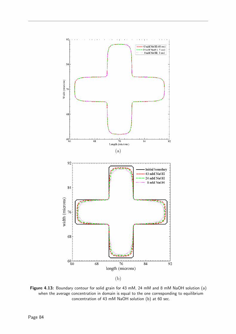
(a)

(b)

Figure 4.13: Boundary contour for solid grain for 43 mM, 24 mM and 8 mM NaOH solution (a)when the average concentration in domain is equal to the one corresponding to equilibrium

concentration of 43 mM NaOH solution (b) at 60 sec.

Page 84

of domain as shown in Fig. 4.10. The shape of the portlandite grain is chosen to include

inner and outer corners, but kept symmetric so that change of geometry can be visually

verified. The domain is initially filled with an aqueous NaOH solution and simulations

were carried out for different molar concentrations of NaOH viz., 8 mM (pH ≈ 11.867, ionic

strength ≈ 7.965× 10−3 at 25C), 24 mM (pH ≈ 12.326, ionic strength ≈ 2.371× 10−2 at

25C) and 43 mM (pH ≈ 12.567, ionic strength ≈ 4.214 ×10−2 at 25 C). All boundaries

are no flux boundaries to simulate a closed system. The amount of portlandite in the solid

grain is 5M (instead of ≈30 M in case of hardened cement paste) to clearly observe the

influence of dissolution on geometrical changes before equilibrium is reached.

Fig. 4.11 shows the evolution of the average aqueous total Ca concentration with time.

The average total Ca concentration at equilibrium corresponds to the equilibrium Ca

concentration. Solutions with a lower NaOH content (lower pH) require a higher amount of

portlandite to be dissolved to reach equilibrium. On the other hand, equilibrium is reached

at the same time for all three cases and the profile of total Ca concentration normalized

with respect to the equilibrium concentration over time coincide with each other as a

consequence of a diffusion-controlled dissolution process (Fig. 4.12). This can be also

confirmed from Fig. 4.13(a) which shows that the portlandite grain boundary for all the

three cases overlap each other when the average concentration in the domain corresponds

to the equilibrium concentration with 43 mM NaOH solution. The final portlandite grain

boundary at the end of simulations for all the three cases is shown in Fig. 4.13(b) which

shows that solutions with lower NaOH content undergoes more dissolution.

4.6.2 Influence of surface area and spatial arrangement

Surface area is an important parameter influencing the dissolution rate of minerals.

However, not only the surface area, but also the spatial arrangement of different mineral

grains determines the average dissolution rate. For example, if two mineral grains are

located close to each other, the narrow channel formed between two grains might reach

local equilibrium, prohibiting further dissolution of the grains from these surfaces. Hence,

surface area and location of mineral grains contribute to average dissolution rate and to

the evolution of microstructure during dissolution.

To illustrate these processes, the cross-shaped grain from the Section 4.6.1 is further

divided into four equal ‘L’ shaped parts as shown in Fig. 4.14, which doubles the surface

area compared to that in the Section 4.6.1. Simulations were carried out for two spatial

arrangements of these grains as shown in Fig. 4.14. In case 2 (Fig. 4.14(a)), grains are

separated from each other forming a narrow channel of 2 µm between them, whereas

in case 3 (Fig. 4.14(b)), they are separated more distantly from each other. Boundary

conditions are similar to those in the previous example. Initial concentration of NaOH

solution is set to 8 mM in the domain.

Page 85

(a) (b)

Figure 4.14: Geometry setup for simulations in section 4.6.2. Region in black represents portlanditegrain. a) referred as case 2, b) referred as case 3 in text

Figure 4.15: Average total Ca concentration showing influence of surface area and relative locationof portlandite grain. The first 6 sec of profile is magnified in inset. Dashed line indicates

equilibrium computed using PHREEQC.

Page 86

Figure 4.16: Total Ca concentration contour at 0.1668 s: a) Case 1, b) Case 2, c) Case 3 ofSection 4.6.2

(a) (b)

Figure 4.17: Boundary contour for solid grains: a) Case 2 of Section 4.6.2, b) Case 3 of Section4.6.2

Page 87

(a) (b)

Figure 4.18: Boundary contour for top-left ’L’ solid grain: a) Case 2, of Section 4.6.2, b) Case 3 ofSection 4.6.2

Fig. 4.15 shows the evolution of the average total Ca concentration with time. In case 2,

the narrow channel between the grains quickly reaches local equilibrium (concentration

gradient inside the narrow channel is close to zero) soon after the start of portlandite

dissolution as indicated in Fig. 4.16(b) which shows the total Ca concentration profile at

time 0.1668 s. This inhibits further dissolution of the inner surfaces. Thus, even though

the total surface area is twice than that in case 1, the accessible reactive surface area is

almost the same as in case 1. Therefore, only small differences in average dissolution rate

and total Ca concentration are observed between cases 1 and 2 (see Fig. 4.15). When the

grain surfaces are sufficiently apart from each other (as in case 3), concentration gradients

exist in all directions (see Fig.4.16c), and hence all faces dissolve faster. This result in a

higher average dissolution rate and shorter time to reach equilibrium for case 3 compared

to cases 1 and 2 (see Fig. 4.15). Fig. 4.17 shows the altered grain shapes for cases 2 and

3 at end of simulation. Fig. 4.18 magnifies the top-left ‘L’ shaped grains for case 2 and

3. Fig. 4.18 clearly shows that inner surfaces do not tend to dissolve in case 2 whereas

all surfaces are dissolving in case 3. This example effectively demonstrates the influence

of surface areas and spatial arrangements of grains on the average dissolution rate and

suggests that in case of complex pore structure such as one of hardened cement paste

heterogeneities might play an important role in determining average dissolution rate.

4.6.3 Influence of pore network on dissolution

To investigate the influence of the pore network characteristics on leaching, a random

porous media consisting of a portlandite mineral as an only reacting phase is considered. In

Page 88

Figure

4.19:

Gen

erat

edp

orou

sm

edia

for

Sec

tion

4.6.

3

Page 89

Table 4.1: Characterization of generated porous media

Cd φport φI Np Amax Amin Amean PR/Ap Deff/D0

Case 1 0.005 0.15 0.0 35 174 6 42.914 0.9786 0.5903Case 2 0.05 0.15 0.2 35 174 6 42.914 0.7856 0.1650Case 3 0.005 0.15 0.0 276 35 1 5.4348 2.2167 0.5701Case 4 0.05 0.15 0.2 276 35 1 5.4348 1.6827 0.1132

particular, the influence of particle size and tortuosity is investigated through 4 cases shown

in Fig. 4.19. The random porous media is generated using the Quartet Structure Generation

Set (QSGS) algorithm [134]. This algorithm requires parameters such as directional

probabilities for growth in a Von Neumann neighbourhood, core probabilities determining

initial number of seeds for growth, the phase fractions and interaction probabilities between

two phase if the growth of phases is correlated to generate random porous media. The

directional probabilities for QSGS algorithm in orthogonal direction is taken as 0.001 and

0.00025 in diagonal directions to ensure exact phase fractions. The core probability for

each case is given in Table 4.1. In all four cases the fraction of portlandite mineral is set

to 0.15. Case 1 and Case 3 consist only of portlandite mineral. To increase tortuosity

in Case 2 and Case 4, an inert phase with fraction of 0.2 was introduced, keeping the

same portlandite mineral phase arrangement as that in Case 1 and Case 3 respectively.

The generated random porous media for all four cases is shown in Fig. 4.19. Table 4.1

summarizes parameters of initial microstructure such as fraction of portlandite (φport),

fraction of inert phase (φI), number of particles of portlandite mineral (Np), maximum

area of portlandite mineral particle (Amax), minimum area of portlandite mineral particle

(Amin), mean area of portlandite mineral particle (Amean), ratio of reactive perimeter (PR)

over total area of portlandite mineral grain (Ap) , and ratio of effective diffusivity of media

to diffusivity of ion in water (De/D0). The simulation domain consists of 100 µm × 100

µm with pore water initially in equilibrium with portlandite. The left boundary was set

to a constant Ca concentration boundary of 0M. Top, bottom and right boundaries were

set as no flux boundaries. Simulations were carried out up to 600s.

Time evolutions of average aqueous Ca concentration and average portlandite concentration

are shown in Fig. 4.20(a) and Fig. 4.20(b) respectively. Whereas a similar rate of dissolution

is obtained for Case 1 and Case 3 (both has a porosity of 0.85), Case 2 has higher rate

compared to Case 4 (both has a porosity of 0.65). Although there is large variation of

PR/Ap between the different cases (Table 1), De/D0 for Case 1 and Case 3 varies by factor

of 1.035, whereas it varies by factor of 1.458 for Case 2 and Case 4. This suggests that

tortuosity has a more pronounced effect than surface area (i.e. particle size) on the overall

dissolution behaviour. Also, lower porosity results in lower De/D0, which leads to lower

dissolution rate. Case 2 and Case 4 has lower dissolution rate compared to Case 1 and

Case 3 which is evident from Fig. 4.20.

Page 90

(a) (b)

Figure 4.20: Time evolution of (a) average Ca concentration and (b) average portlanditeconcentration. Averages are taken over phase volume

Figure 4.21: Ca profiles at the end of simulation (600s)

Page 91

Figure 4.22: Time evolution of mean location of boundary where Ca is greater than 19mM

Figure 4.21 shows the Ca concentration contours at 600 s. the dissolution front moves

slower for Case 2 and Case 4 compared to Case 1 and Case 2 with Case 4 the slowest

front movement of all cases. To quantify front movement over time, the front position was

defined as the mean distance along the horizontal axis at which the concentration is greater

than 19mM. Fig. 4.22 shows this front position over time. There are smaller differences

in front movement between Cases 1 and 2 as compared to Cases 3 and 4. Moreover for

lower porosities (Cases 2 and 4), the front movement is slower compared to the cases with

higher porosities (Cases 1 and Case 3) as shown in Fig 4.22.

The results suggest that the tortuosity of the porous media is more significant than the

particle shape and the surface area for dissolution in random porous media. Further it

indicates that the initial transport properties of media such as porosity and tortuosity

have a dominant influence on dissolution behaviour.

4.7 Conclusions

In this chapter, extension of LB schemes for pore-scale and multilevel porous media

to incorporate single component and multi-component reactive transport processes are

presented. In case of multi-component reactive transport scheme a pseudo-homogeneous

treatment is proposed to deal with heterogeneous reactions. Even though, the benchmark

shows that this approach is less accurate compared to the conventional approach to treat

heterogeneous reactions as boundary conditions, flexibility the proposed approach offers

outweighs this drawback. The main advantage of a pseudo-homogeneous treatment is

Page 92

the ability to treat both homogeneous and heterogeneous reactions in same way thus

replacing homogeneous and heterogeneous reactions with a single source/sink term. This

allows for the coupling of LB schemes for pore-scale and multilevel porous media with

external geochemical codes which have been developed over several decades. This makes

the approach more versatile to incorporate new geochemical reaction networks. In this

work, a successful coupling of LB schemes with geochemical code PHREEQC have been

presented for the first time. This coupling has been validated with wide range of benchmark

examples. An approach to update the boundary of non-diffusive solid phase as a result of

dissolution or precipitation has been presented and validated. It has been found that the

changing of boundary at threshold volume fraction of 0.5 is more accurate than updating

the boundary on complete dissolution or precipitation as proposed by Kang et al. [45]

which is commonly used in literature.

A series of examples highlighting the influence of parameters such as solution composition,

surface area and location of mineral phases and pore network characteristics on disso-

lution of portlandite have been presented. Under diffusive transport conditions and a

thermodynamic equilibrium approach, different initial pH conditions do not influence the

overall reaction rate. However lower pH values increase the amount of portlandite dis-

solved resulting in smaller grains at the end of simulation. Further for diffusion controlled

dissolution, spatial arrangement of mineral grains is more important that the surface area.

The spatial arrangement of grains may cause local equilibrium in certain parts of the

domain inhibiting local dissolution processes at the grain surface.

Finally, in order to study influence of pore network on portlandite dissolution four cases

consisting of random porous media with portlandite as reacting phase were presented. All

four cases had the same fraction of portlandite phase but differ in particle sizes or total

porosity (by introducing inert material). The latter also increased the tortuosity. The

results show that characteristics of porous media affecting ion transport such as tortuosity

and porosity have a more pronounced effect on dissolution compared to particle size and

surface area for diffusion controlled dissolution.

The results from these simple examples highlights the importance of ion transport at

the pore-scale as a crucial factor for determining the overall dissolution rate. In a real

microstructure of hardened cement paste, the results from these simplified simulations

suggest that the heterogeneity (spatial location of mineral phases) might play important

role in determining the average dissolution rate and the evolution of cement paste pore

structure during leaching.

Page 93

Part II: Applications to cement based materials

Page 95

CHAPTER 5

Critical appraisal of experimental data and models for diffusivity of

cement paste

5.1 Introduction

Varieties of degradation processes of cement based materials such as chloride ingress and

corrosion, sulphate attack, carbonation and calcium leaching are associated with the

transport of ions and gases. One of the important transport mechanisms of ion and gases

is diffusion which refers to the transport of matter under concentration gradient. The

rate of diffusion is characterized by the diffusion coefficient or commonly referred to as

diffusivity. Diffusivity is an important parameter for modelling degradation processes for

practical applications such as contaminant transport in cementitious barriers, assessment

of long-term behaviour of nuclear waste disposal systems based on cementitious materials,

prediction of rebar corrosion in civil concrete structures. Diffusivity is also a key durability

parameter to define service life of concrete structures [135]. Diffusivity of a porous media

at the macroscopic scale is given as [136]

De =θD0δ

ζ2(5.1)

De is the diffusivity of ion/gas in porous media also known as effective diffusivity, D0 is the

diffusivity of the ion/gas in pore water, θ is the water content which is equal to porosity

for saturated media; δ is the constrictivity; and ζ is the geometric tortuosity factor. The

ratio (De/D0) is also referred to as relative diffusivity of the media [137]. Alternatively

Page 97

Eq. (5.1) can also be represented as [136]

De = θζaD0 (5.2)

ζa is the apparent tortuosity factor. In case of sorption/binding of ions to porous media

for e.g. binding of chloride ions in cement based materials, diffusivity is given as [136].

Da =θD0δ

Rdζ2(5.3)

Da is the diffusivity accounting for retardation caused by binding/sorption also known as

apparent diffusivity and Rd is the retardation factor. Geometric tortuosity factor takes

into account that diffusion occurs only through the connected pathway. Constrictivity

accounts for the narrowing of pores thus restricting the diffusion of species through the

pore. Constrictivity depends on the ratio of the diameter of the diffusing particle to the

pore diameter. Moreover phenomena such as anion exclusion and influence of adsorbed

layer on diffusion is also lumped into constrictivity [138]. Thus both constrictivity and

tortuosity depend on the morphology of the media. The morphology of the cement based

material depends on several factors such as water to cement ratio (w/c), admixtures,

initial composition of cement clinkers, curing conditions and degree of hydration and hence

determination of diffusivity and its prediction is a formidable task.

During last decade efforts has been laid in understanding the process in diffusion and

to measure diffusion coefficients. Varieties of methods have been proposed to measure

the diffusivity and none of them seems to be univocally accepted. Moreover, different

models have been developed to predict the diffusivity of cement based materials. In this

chapter an overview on these developments is presented and in particular differences and

similarities between different experiments and modelling approaches are highlighted. The

scope of this chapter has been limited to steady state diffusivity (i.e. apparent diffusivity

not considered) under saturated conditions for ordinary Portland cement (opc).

Section 5.2 gives an overview of experimental data obtained using different techniques

and through collection of large amount of experimental data provides perspectives on

differences in the values of diffusion coefficients obtained by different methods. Section

5.3 presents an overview on existing diffusivity models for opc. Section 5.4 presents a

comparative analysis of cement paste diffusion models discussed in section 5.3. In section

5.5, summerize details on efforts made by different researchers for estimating diffusivity

from the cement paste microstructures.

Page 98

5.2 Comparison of relative diffusivities obtained by

different techniques

The experimental methods used to measure diffusion coefficient can be grouped into four

types: (i) through-diffusion based on measuring fluxes; (ii) in-diffusion based on measuring

concentration profiles in the sample; (iii) electro-migration experiments, either by through-

or in-diffusion, in which ion diffusion is accelerated by an electric field; and (iv) techniques

in which proxy variables are used to determine diffusivity, e.g. electric resistivity techniques.

Overview on these techniques can be found in [8]. Data for diffusion experiments on cement

pastes as reported by different researchers using these techniques are compiled in this

section. The data include measurements carried out using through-diffusion experiments

for tritiated water (HTO) [5, 7, 139–142] and dissolved gases such as helium [8], oxygen

[6, 141]; and electrical resistivity [9, 143–145]. Only the steady state diffusion coefficients

of chloride ion determined by electro-migration technique [6, 146, 147] were included in

this comparison as the chloride is known to bind with the hydration product and as a

result non-steady state chloride diffusion varies with time.

Composition of the cement for the collected data is summarized in table 5.1. For the

references where no direct values of capillary porosity are available, the capillary porosity(φ)

is computed using Power’s model [148].

φ =w/c− 0.36α

w/c + 0.32(5.4)

where α is the degree of hydration. In cases where the degree of hydration was not

available it was assumed that the paste has been hydrated to maximum achievable degree

of hydration. The maximum degree of hydration (αmax) was computed using relationship

given in [5].

αmax = 0.239 + 0.745 tanh[3.62(w/c− 0.095)] (5.5)

Indeed based on the curing conditions used for majority of experiments (summarized in

table 5.2) it can be assumed that the maximum degree of hydration has been attained.

The compiled data is summarized in table 5.3 and table 5.4.

The relationship between relative diffusivity and w/c and capillary porosity for the collected

data is shown in Fig. 5.1(a) and Fig. 5.1(b) respectively. Increase in relative diffusivity

with respect to higher w/c and capillary porosity is consistent for all reported data. The

relation of the relative diffusivity with w/c shows more scatter than the relation with

capillary porosity. This is due to the fact that at a given w/c, the degree of hydration

achieved might vary for reported data, which in turn can results in different porosities.

Regardless of the use of different experimental techniques and authors, all reported data

are fitted well to the exponential relationship correlating the relative diffusivity with

Page 99

Table 5.1: Cement composition of the collected data

Reference Bouges composition (in %) Fineness(m2/Kg)C3S C2S C3A C4AF

Phung [8] 65.43 15.14 9.19 10.24 435Ma et al. [9] 62.6 17.03 9.73 10.06 -

Yamaguchi et al. [142] 51.79 26.72 11.53 9.95 -Bejaoui and Bary [5] 67.36 21.46 3.75 7.43 310.5Castellote et al. [141] 61.18 15.98 12.21 10.63 -

Delagrave et al. [7](w/c=0.45) 68.7 5.8 7.4 5.1 461.6Delagrave et al. [7] (w/c=0.25) 68.7 6.9 7.7 5.4 535.1

Ngala and Page [6] 54.81 25.7 10.71 8.77 345Christensen et al. [145] 73.48 19.96 5.36 1.19 -

Oh and Jang [146] 30.0 40.5 11.0 9.7 -Sun et al. [147] 55.5 19.1 6.5 10.1 -

Table 5.2: Curing conditions for the collected data

Curing conditions ReferenceFor 28 days in sealed condition in a controlled tempera-ture of 22C± 2C

Phung [8]

The samples were cured at 50C under deionized wa-ter until peak of in XRD of unhydrated cement phasedisappears

Yamaguchi et al. [142]

Samples are cured in saturated lime water incoroporatingsodium and potassium hydroxide during 12 months

Bejaoui and Bary [5]

Samples are cured for 28 days under water. They werestored for 1 month immersed in a saturated Ca(OH)2

solution

Castellote et al. [141]

The specimens were demolded and immersed in limesolution for 3 months

Delagrave et al. [7]

After curing at 22C for 2 weeks and immersed in 35mMNaOH solution. They were then stored in a curing roomat temprature of 38± 2C for 10 weeks

Ngala and Page [6]

Cured for 28 days in a 100% relative humidity chamberat 25C

Numata et al. [139]

Cured at 20C till test was performed Oh and Jang [146]The samples were placed in a room at a temperature of20 C for 24 h and then moved to a standard curing room(temperature of 20± 3C, relative humidity above 95 %).After three days of curing, the samples were removedand split into several parts. Finally, the samples weretaken out for measurement of their degree of hydrationand porosity at the required standard age

Sun et al. [147]

Page 100

Table 5.3: Summary of data of diffusion coefficient collected from literature: electric resistivitytechnique

Reference w/c Degree ofhydration

Capillaryporosity

De/D0(×10−2)

Ma et al. [9] 0.3 0.28 0.321∗∗ 2.850.431 0.24∗∗ 1.630.522 0.18∗∗ 1.520.61 0.13∗∗ 1.340.65 0.11∗∗ 1.30

0.4 0.33 0.39∗∗ 5.360.51 0.30∗∗ 2.910.631 0.24∗∗ 2.360.70 0.21∗∗ 2.010.72 0.2∗∗ 1.76

0.5 0.36 0.45∗∗ 9.500.56 0.37∗∗ 5.300.67 0.32∗∗ 3.880.74 0.29∗∗ 2.670.79 0.27∗∗ 2.01

Tumidajski et al. [143] 0.25 0.54∗∗∗ 0.10 0.1040.3 0.63∗∗∗ 0.12 0.3720.4 0.6∗∗∗ 0.26 2.040.5 0.68∗∗∗ 0.31 2.420.8 0.42∗∗∗ 0.58 10.51 0.65∗∗∗ 0.58 10.5

Taffinder and Batchelor[144]

0.4 0.84∗ 0.137∗ 0.476

0.5 0.91∗ 0.211∗ 0.5810.6 0.946∗ 0.282∗ 1.030.7 0.966∗ 0.345∗ 1.670.8 0.975∗ 0.401∗ 1.820.9 0.98∗ 0.449∗ 2.631.0 0.982∗ 0.49∗ 3.70

Christensen et al. [145] 0.5 0.611∗∗ 0.31∗∗ 2.870.511 0.36∗∗ 3.520.491 0.37∗∗ 4.310.451 0.39∗∗ 5.890.431 0.40∗∗ 7.070.391 0.42∗∗ 9.220.311 0.46∗∗ 16.30.291 0.47∗∗ 20.90.211 0.51∗∗ 35.20.171 0.53∗∗ 39.50.091 0.57∗∗ 43.00.011 0.61∗∗ 45.6

∗Degree of hydration is taken as maximum degree of hydration computed using equation 5.5 and

porosity computed using equation 5.4∗∗porosity was computed using relationship given in ref [149]∗∗∗Degree of hydration computed using equation 5.4

Page 101

Table 5.4: Summary of data of diffusion coefficient collected from literature: Through diffusion andelectro-migration techniques

Reference Technqiue/Tracer

w/c Degree ofhydration

Capillaryporosity

De/D0(×10−2)

Phung [8] Helium 0.425 0.85∗∗∗ 0.16 0.321Sun et al. [147] electro

migration0.23 0.573∗ 0.04∗ 0.0696

0.35 0.734∗ 0.13∗ 0.22030.53 0.861∗ 0.26∗ 0.723

Yamaguchi et al. [142] HTO 0.45 0.908∗∗∗ 0.16 0.6380.6 0.926∗∗∗ 0.29 2.050.75 0.953∗∗∗ 0.38 3.88

Bejaoui and Bary [5] HTO 0.25 0.62∗ 0.048∗ 0.02510.3 0.71∗ 0.072∗ 0.05050.35 0.782∗ 0.103∗ 0.1220.38 0.817∗ 0.123∗ 0.1460.4 0.84∗ 0.137∗ 0.1640.42 0.856∗ 0.152∗ 0.1780.45 0.879∗ 0.174∗ 0.2390.5 0.91∗ 0.211∗ 0.4040.6 0.946∗ 0.282∗ 0.6960.65 0.958∗ 0.315∗ 0.937

Oh and Jang [146] electromigration

0.35 0.673∗∗∗ 0.161 0.254

0.45 0.788∗∗∗ 0.225 0.4430.55 0.83611∗∗∗ 0.286 1.061

Castellote et al. [141] oxygen 0.4 0.84∗ 0.137∗ 0.453Delagrave et al. [7] HTO 0.45 0.879∗∗∗ 0.22 0.439

0.25 0.55∗∗∗ 0.09 0.0281Ngala and Page [6] oxygen 0.4 0.84∗ 0.137∗ 0.449

0.5 0.91∗ 0.211∗ 0.4980.6 0.946∗ 0.282∗ 0.6530.7 0.966∗ 0.345∗ 1.04

Ngala and Page [6] electromigration

0.4 0.84∗ 0.137∗ 0.2703

0.5 0.91∗ 0.211∗ 0.50680.6 0.946∗ 0.282∗ 0.81080.7 0.966∗ 0.345∗ 1.4864

Revertegat et al. [140] HTO 0.37 0.625∗∗∗ 0.21 0.2Numata et al. [139] HTO 0.4 0.831∗∗∗ 0.14 0.228

0.5 0.774∗∗∗ 0.27 0.4240.55 0.851∗∗∗ 0.28 0.504

∗Degree of hydration is taken as maximum degree of hydration computed using equation 5.5 and

porosity computed using equation 5.4∗∗porosity was computed using relationship given in ref [149]∗∗∗Degree of hydration computed using equation 5.4

Page 102

Figure

5.1:

Rel

ativ

ed

iffu

sivi

tyvs

.(a

)w

/can

d(b

)ca

pill

ary

por

osit

y-

dat

ais

fitt

edto

exp

onen

tial

rela

tion

ship

(bol

dso

lidlin

es);

shad

edre

gion

sre

pres

ent

the

fact

orof

five

,tw

oan

dfo

ur

bou

nd

sfo

rth

eex

pon

enti

alre

lati

onsh

ipfi

tted

wit

hd

ata

from

elec

tric

alre

sist

ivit

y,el

ectr

o-m

igra

tion

and

thro

ugh

diff

usi

on,

resp

ecti

vely

.

Page 103

w/c or capillary porosity. However the data obtained by electrical resistivity shows most

scatter (within factor of five bound1), whereas electro-migration data shows least scatter

(within factor of two bound). Spragg et al. [150] have analysed in detail different factors

affecting electrical resistivity measurements. They reported that several key parameters

such as type of setup, temperature, sample storage and conditioning, frequency of current

at which measurements are carried out, and the resistivity of pore water solution may

result in large variations of the relative diffusivity obtained by the electrical resistivity

measurements. The relative diffusivity obtained from electrical resistivity measurement is

also higher than the ones from electro-migration and through-diffusion. The difference

seems to diminish with the increase of w/c or capillary porosity. When the w/c is larger

than 0.4, the differences between the different techniques diminishes.

5.3 Effective diffusivity models

In this section different constitutive relationships to predict diffusion coefficients are

reviewed. Many relationships have been proposed to describe the link between diffusivity of

cement paste and parameters such as porosity, w/c and volume fractions of different phases.

These relationships can be broadly classified into empirical approaches, relationships derived

from numerical models and analytical relationships which are based on effective media

theories. Further classification can be made for models based on effective media theory into

models considering morphology of cement paste in simplified form and models taking into

account in details the morphological characteristics of cement paste. These relationships

are summarized in Appendix F.

The empirical relationships between parameters (e.g. porosity, w/c) which link morphology

and effective diffusivity through a set of constants are determined by fitting this relationship

with the experimental data. The empirical relationships do not directly account for the

morphology and connectivity of the pore structure and these considerations are lumped in

fitting coefficients. Some of these relationship have been directly adapted from the soil

science. For instance, Archie’s power relationship [151] which was preliminary proposed

for rocks and sand has been adapted for cement paste. Archie’s relationship is originally

presented in terms of total porosity. For cementitious materials it is usually assumed

that the major effect on transport properties is due to capillary porosity and hence some

authors [137, 146] express Archie’s relationship in terms of capillary porosity. Moreover,

porosity for cement paste is often determined by a Mercury Intrusion Porosimetry (MIP)

which covers mainly capillary pore range [152]. Hence in this chapter all empirical

relationships including Archie’s relationship have been expressed in terms of capillary

porosity. Applicability of Archie’s relationship to cementitous materials has been argued

1The factor of five bound refers to the area in between the line drawn by multiplying and dividing fivewith the best fit value

Page 104

Table 5.5: Values of coefficients and power for Archie’s relationship as derived by different authors.a and n are coefficient and power which are to be fitted for Archie’s relationship.

Reference a nTumidajski et al. [143] 1.89 2.55Tumidajski et al. [143] using data of Christensen et al. [145] 0.14 4.8Tumidajski et al. [143] using data of Taffinder and Batchelor [144] 7.71 3.32Yamaguchi et al. [142] 0.18 0.94

by some authors [137, 145, 153]. Moreover, the fitting parameters obtained by different

authors for Archie’s relationship vary substantially. These values are summarized in Table

5.5. Despite these limitations, Archie’s relationship is often used to simulate reactive

transport processes in cement [13, 154]. To alleviate the inability of Archie’s relationship

to account for the percolation threshold Winsauer et al. [155] proposed the extension

which sets the diffusivity to zero when the porosity is smaller than the threshold porosity

(φc). For cement paste, the fitting parameters for this relationship have been obtained

by Lee et al. [156]. The effective diffusivity can also be expressed as the exponential

function of the porosity instead of power relationship as suggested in Refs. [139, 153, 157].

The exponential function is also used to describe the relationship between w/c ratio and

effective diffusivity [158].

Garboczi and Bentz [137] proposed relationship between relative diffusivity and capillary

porosity based on numerical computation of diffusivity from virtual microstructures of

cement paste. Computation of diffusivity from virtual microstructure allows distinguishing

contributions of different diffusive phases viz. C-S-H and capillary pores to diffusion. The

first term in their relationship represents the contribution from the percolating fraction of

capillary pores. The second term represents contribution of non-percolating capillary pores

and C-S-H phase. The last term is the contribution of C-S-H when capillary porosity is

zero. Through numerical simulations on virtual microstructure of hydrating C3S paste they

determined the values for the coefficients a1, a2 and a3 as 1.8, 0.07 and 0.001 respectively

(for mathematical expression see appendix F). The threshold porosity (φc) was determined

as 0.18. Bentz et al. [159] re-determined the coefficients a1, a2 and a3 for cement paste as

1.7, 0.03, and 0.0004 respectively. The threshold porosity for cement paste was determined

as 0.2. The threshold porosity computed from the virtual microstructure of cement paste

has been found to be independent of w/c. However, it strongly depends on the resolution

of the microstructure and microstructure model used [160–162] and hence percolation

threshold can be considered as an additional parameter that can be adjusted. Furthermore,

many models discussed later in this paper base the percolation threshold on work of

Garboczi and Bentz [137] and hence the percolation threshold is classified as an unknown

parameter in this chapter.

The models presented till now are either empirical or have been derived from numerical

computations. Alternatively the morphology of cement paste can be conceptualized into

Page 105

a simple geometrical configuration for which analytical solution or theoretical model

can be devised. These theories are known as effective media theory. The simplest

geometrical configuration for which analytical solution exist is arranging different phases

of the multiphase material such as cement paste in series or parallel. Bejaoui and Bary

[5] presented a set of series/parallel configurations, to predict diffusivity of the cement

paste as shown in Fig. 5.2. In their approach the percolating diffusive phases are placed

in parallel. The non-percolating phases are placed in series. The degree of percolation was

computed based on volume fraction. They assumed that the phase starts to percolate once

its volume fraction is 15% and the amount of percolating fraction increases linearly and

becomes fully percolated at 25% volume fraction. This function for degree of percolation

is inspired from the analysis on CEMHYD3D generated microstructures reported by Bentz

et al. [159]. Additionally to account for the tortuosity of capillary pores they used an

exponential law. The tortuosity of LD and HD C-S-H phase and mixed fraction of LD

C-S-H and capillary pores was taken into account using the effective media theory for

single coated spheres [163]. The porosity of LD and HD C-S-H was taken as 20% and 31%

respectively according to Jennings model [22]. The phase fractions needed for their model

is determined using the Tennis and Jennings hydration model [15]. They determined the

diffusion coefficient of LD C-S-H and HD C-S-H as 9 × 1012 m2/s and 1 × 1012 m2/s,

respectively, for HTO by fitting the experimental data.

Another set of configuration for which theoretical models exist are the well-defined inclusions

(such as spheres, cylinders, ellipsoids) distributed randomly throughout a matrix material.

The basic idea behind these models have been discussed in appendix G. Several cement

paste models have been proposed wherein cement paste has been conceptualized to be

composed of inclusions in a matrix. Pivonka et al. [164] applied the differential media

approximation to predict the effective diffusivity of cement paste. The cement paste

morphology is conceptualized as a media composed of non-diffusive phase as spherical

inclusions in matrix of capillary pores. The diffusion through gel (C-S-H) pores is thus

neglected. Based on the comparison with the results of experiments for steady state

chloride diffusivity, they found that the values obtained from differential effective media

theory an one order higher than that of experiments. Hence they suggested to decrease the

diffusivity of pore solution by factor of 10. They attributed the choice of lower diffusivity

in the pore solution of cement paste to the higher viscosity of the pore solution which

is due to the restructuring of water molecules along the charged pore surfaces. Under

these assumptions the differential approximation reduces to Archie’s law with values of

coefficient and power as 0.1 and 1.5 respectively. Christensen et al. [145] have shown that

for electric resistivity measurements, differential approximation provides good correlation

only at early stages of hydration when capillary porosities are greater than 50%. However,

at later stage of hydration, differential scheme breaks down. Oh and Jang [146] applied

generalized effective media approximation to predict effective diffusivity of cement paste.

Page 106

Figure 5.2: Simplified equivalent systems proposed by Bejaoui and Bary [5] for HCP

Page 107

They considered that the cement paste consists of inclusions capillary pores and diffusive

solid (C-S-H) in matrix of equivalent homogeneous media. According to this model, for the

porosity smaller than threshold capillary porosity, diffusion occurs through the diffusive

solid. They assumed threshold capillary porosity as 0.17. They determined the relative

diffusivity of this solid phase by fitting with the experimental data as 2.0 × 10−4. The

relationship derived from the generalized effective media theory takes a similar form as

that of modified Archie’s relationship proposed by Winsauer et al. [155] when diffusivity

of solid phase is zero. Therefore, modified Archie’s law can also be viewed as a specific

case of generalized effective media theory.

Models based on effective media theory so far described considered a very simplistic view

on morphology of cement paste. Several models have been proposed which account for

more detailed morphological description of cement paste. The cement paste morphology is

represented in several levels and the effective media theories are then utilized for obtaining

effective diffusivity at each level. Bary and Bejaoui [165] conceptualized morphology

of cement paste as a three coated spheres with the core at the centre and three layers

around this core viz., inner, intermediate and outer layers. The clinker forms the core

and hydration products are represented as layers around the clinker phase. The hydration

products are divided into two layers (inner and outer layers), in which other minor phases

(portlandite (CH) and aluminate phases (AFm)) are inclusions. The inner layer is formed

of HD C-S-H whereas outer layer is formed of LD C-S-H. The outer layer further contains

inclusions of more diffusive capillary pores. They further divided outer layer into two

parts where one part consists of non-percolated capillary pores and the other part contains

percolated capillary pores. They assumed the fractions of non-percolated capillary pores

as 8%. Both intermediate and outer layers have equal amount of CH and AFm inclusions.

The fraction of portlandite and aluminate phases in inner and outer layer are distributed

in the same proportion as the fractions of HD and LD C-S-H in cement paste. The

effective diffusivity of this configuration is determined using the effective media theory

for multi-coated spheres proposed by Milton [166]. This theory is based on self-consistent

approximation. According to this theory, effective diffusion coefficient of the microstructure

(De,n) consisting of n layer multi-coated sphere can be determined iteratively, wherein at

each iteration the effective media is composed of single coated spheres with core consisting

of effective media of previous iteration surrounded by the layer of the current iteration

using following equation [166]

De,n = Dn +

(1− φn∑n

i=1 φi

)[1

De,n−1 −Dn

+1

3Dn

φn∑ni=1 φi

]−1

(5.6)

Where De,n is the effective diffusivity determined for nth layer [L2,T−1]; φi is the fraction

of ith layer and De,n−1 is the effective diffusion coefficient of assembly of multi-coated

spheres consisting of n − 1 layers. The diffusion coefficient for inner and intermediate

Page 108

layers in Bary and Bejaoui [165] model are then determined by Maxwell approximation

and diffusion coefficient of external layer is determined using self-consistent scheme to

better represent the effect of percolation. For intermediate and outer layer additionally

they assume that DintCSH/D0 and Dout

CSH/D0 as zero to simplify the relationships. However,

this assumption is not essential. The volume fractions of different phases needed are

determined using Tennis and Jennings model [15]. Diffusivity of inner and outer C-S-H

matrix were determined by fitting with the experimental data of Bejaoui and Bary [5] as

3.4× 10−12 m2/s and 8.3× 10−13 m2/s, respectively, for HTO.

Similar conceptualization has been made by Stora et al. [167] for cement paste morphology.

However they did not divide the outer layer further in two parts as in case of Bary and

Bejaoui [165]. Diffusivity of both layers were determined using Maxwell approximation.

Moreover in order to obtain the effective diffusivity of LD and HD C-S-H they applied

the mixed coated sphere assemblage model (MCSA) [168] which allows to capture sudden

variations of effective diffusivity caused by percolation effects in a better way than self-

consistent scheme. The MCSA model requires an additional fitting parameter known as

the geometric parameter (f) which they determined as 0.805 and 0.546 for HD C-S-H and

LD C-S-H respectively based on comparison with experimental data. This model has been

further extended to simulate the leaching of cement paste [169]. Dridi [170] also utilized the

effective media theory for assembly of multi-coated spheres to compute effective diffusivity

of cement paste. He used similar morphological conceptualization as Stora et al. [167].

However, in case when LD C-S-H volume fractions are smaller than percolation threshold

which is the case for low w/c, he represented cement paste as single coated spheres with LD

C-S-H as inclusions in the layer of HD C-S-H. Similar to Stora et al. [167] the diffusivity of

inner and outer layer is computed using generalized Maxwell approximation. Moreover in

order to account for percolation behaviour of capillary pores he used self-consistent scheme

for outer layer when capillary pores percolate. The percolation threshold for capillary

pores was assumed to be 15%. He used the diffusivity of LD and HD C-S-H as 6.5× 1012

m2/s and 1.25× 1012 m2/s by fitting with experimental results of Bejaoui and Bary [5]

rather than using MCSA model as in case of Stora et al. [167]. These values are in the

similar range as the one fitted by Bary and Bejaoui [165].

Liu et al. [171] represented the morphology of cement paste in rather different way.

They considered cement paste morphology in three levels . At level I they assumed the

representation of two types of C-S-H, LD C-S-H and HD C-S-H. Both LD and HD C-S-H

are composed of non-diffusive spherical solid phase as inclusions in the gel pore space.

At level II the porous C-S-H gel is composed of spherical inclusion of HD C-S-H and

capillary pores smaller than 1 µm in the matrix of LD C-S-H. Finally at level III the HCP

is assumed to consist of spherical inclusion of unhydrated cement, portlandite, aluminates

and capillary pores in the matrix of porous C-S-H gel. The diffusivity of LD and HD

C-S-H at level I is determined using differential effective media scheme. The diffusivity

Page 109

Table 5.6: Values of unknown parameter used for different relative diffusivity models of cementpaste.The mathematical expression for this models can be found in appendix F.

Reference/ Model Parameters usedArchies relationship a : 0.0462, 0.1158, 0.5385 for electro migration, through-

diffusion and electric resistivity respectivelyn: 1.3916, 2.0609, 2.3366 for electro migration, through-diffusion and electric resistivity respectively

Exponential form a: 0.0006, 0.0003 and 0.0021 for electro migration,through-diffusion and electric resistivity respectivelyn: 9.7627, 11.507 and 8.2079 for electro migration,through-diffusion and electric resistivity respectively

Exponential form with re-spect to w/c

a: 0.002,0.00007 and 0.0002 for electro migration,through-diffusion and electric resistivity respectivelyn: 3.4779 , 8.2253 and 6.3193 for electro migration,through-diffusion and electric resistivity respectively

NIST model [159] a1: 1.7, a2: 0.03, a3: 0.0004 and φc: 0.2Generalized self-consistentscheme [146]

Ds: 2× 10−5D0 , n: 2.7 and φc: 0.17

Bejaoui and Bary [5] DLD−CSH : 4.0179×10−3D0, DHD−CSH : 4.4643×10−4D0

Bary and Bejaoui [165] DLD−CSH : 1.7× 10−3D0, DHD−CSH : 4.15× 10−4D0

Stora et al. [167] fLD−CSHgp : 0.675, fHD−CSHgp : 0.761

Dridi [170] DLD−CSH :2.9018×10−3D0, DHD−CSH : 5.35714×10−4D0

Liu et al. [171] Dgp: 1.8634× 10−2D0

at level II and level III are determined using Maxwell approximation and self-consistent

scheme respectively. They determined the diffusivity of ions in gel pores through inverse

analysis. For chloride ions they determined the value of diffusivity of ions in gel pores

as 3× 10−11 m2/s. The volume fractions of different phases where determined using the

hydration model proposed by Bernard et al. [172]. The porosity of LD C-S-H and HD

C-S-H in their model were kept constant for different w/c with values as 0.37 and 0.24

respectively which is based on colloid model of C-S-H proposed by Jennings [23].

5.4 Comparison between effective diffusivity models

In this section comparisons are carried out for the models to obtain diffusivity as presented

in previous section. The parameters needed for these relationships are taken as the one

suggested in the respective references and are summarized in Table 5.6. For empirical

relationships discussed in section 5.3 it is relevant to compare the quality of the relationship

rather than their predictive capabilities. Hence for these relationships unknown parameters

are first calibrated for experimental data collected in section 5.2 and then compared with

the experimental data. The parameters of the calibrated model are summarized in Table

5.6. For models which require volume fractions of different phases the comparisons were

Page 110

Table 5.7: Volume fractions (in %) of different phases of cement paste computed using Tennisand Jennings hydration model [15] for experiments used to compare models considering detailedmorphological aspects of cement paste

refe

ren

ces

w/c

Deg

ree

of

hyd

rati

on

clin

kers

por

tlan

dit

eal

um

inat

esca

pil

lary

poro

sity

HD

C-S

-HL

DC

-S-H

Ele

ctro

-mig

rati

on

Su

net

al.

[147

]0.

230.5

73

22.3

10.8

317

.19

4.5

35.7

58.

36

0.35

0.7

34

9.38

12.4

119

.37

10.

79

31.8

617

.45

0.53

0.8

61

2.66

10.9

217

.42

20.

01

1040

.84

Oh

an

dJan

g[1

46]

0.35

0.6

73

10.1

17.

1228

.04

7.3

30.6

416

.79

0.45

0.7

88

4.91

6.77

25.0

112.

28

20.6

730

.37

0.55

0.8

36

2.46

6.33

22.0

917.

27.

55

44.3

6

Th

rou

gh-d

iffu

sion

Del

agra

veet

al.

[7]

0.45

0.8

79

4.93

15.7

914

.67

13.

669

620

.63

30.3

1

0.25

0.5

521

.21

14.5

214

.84

4.4

291

35.9

451

9.05

Yam

agu

chi

etal.

[142]

0.45

0.9

08

4.87

10.6

23.1

713.

269

419

.47

28.6

1

0.6

0.9

26

1.79

9.21

19.6

320.

714

99.

48

47.6

9

0.75

0.9

53

0.83

8.05

16.8

527.

318

10

43.3

9

Ngal

aan

dP

age

[6]

0.4

0.8

46.

9911

.33

21.9

310.

44

26.0

923

.02

0.5

0.9

13.

4410

.61

20.2

515.

713

.74

36.2

6

0.6

0.9

46

1.79

9.69

18.0

320.

50.

97

49.0

2

0.7

0.9

66

1.04

8.84

16.2

424.

97

048

.91

Phu

ng

[8]

0.42

50.8

55.

8313

.18

19.4

812.

71

22.9

25.9

1

Ele

ctri

cal

resi

stiv

ity

Ma

etal.

[9]

0.3

0.5

22

24.3

9.05

1516.

95

22.6

12.1

6

0.3

0.6

119

.78

10.7

317

.65

11.

927

.63

12.3

2

0.3

0.6

517

.71

11.5

18.8

39.6

430

.08

12.2

3

0.4

0.5

121

.41

7.58

12.5

628.

33

14.6

15.5

1

0.4

0.6

31

16.0

69.

5715

.721.

918

.45

18.3

1

0.4

0.7

013

.01

10.7

217

.41

18.

29

20.7

619

.81

0.4

0.7

212

.13

11.0

517

.89

17.

25

21.4

420

.23

0.5

0.5

616

.83

7.36

12.1

733.

88

9.74

20.0

2

0.5

0.6

712

.57

8.95

14.6

228.

38

11.0

224

.46

0.5

0.7

49.

869.

9816

.124.

911

.75

27.4

1

0.5

0.7

97.

9310

.71

17.1

222.

43

12.2

329

.58

Page 111

Archie's relationshipExponential relationshipExponential relationship (w/c ratio)

simul

ated

(De/D

0)

10−5

10−4

0.1

1

experimental (De/D0)10−5 10−4 10−3 0.01 0.1 1

Figure 5.3: Comparison of relative diffusivity obtained from empirical relationships and experimentaldata. Marker colours represent different experimental techniques. Blue, red and green represents

through-diffusion, electro migration, and electric resistivity respectively. Shaded green regionshows factor of two bound and dashed line shows factor of five bounds.

carried out only for a selected set of experimental data as given in Table 5.7. Care has been

taken that the experimental data selected does not include the ones which has been used

to calibrate these relationships. The volume fractions of different phases were computed

using Tennis and Jennings hydration model [15] and reported in Table 5.7. For Stora et al.

[167] and Liu et al. [171] additionally porosity of LD C-S-H and HD C-S-H is needed. The

porosity of LD C-S-H and HD C-S-H was taken as 0.37 and 0.24 respectively which is

based on colloid model of C-S-H proposed by Jennings [23]. The parameters for Stora

et al. [167] were recalibrated as these porosity values are different from the one used in

their paper.

Fig. 5.3, Fig. 5.4, and Fig. 5.5 shows the comparison of the relative diffusivity obtained

using different relationships for effective diffusivity and experimental data. Alike models

are grouped together in each figure. For instance in Fig. 5.3 all the empirical relationships

are compared with experimental data. In Fig. 5.4 models which account for morphological

nature of cement paste in simplified way and express the relationship solely in terms of

capillary porosity i.e. NIST model [137] and Oh and Jang model [146] based on generalized

effective media theory are compared with experimental data. In Fig. 5.5 models which

take into account detailed morphological aspects of cement paste are compared with the

experimental data. Table 5.8 summarizes the percentage of data for which the relative

diffusivity is within factor of two bounds. This serves as a good indicator to quantitatively

Page 112

NIST modelOh and Jang (2004)

simul

ated

(De/D

0)

10−5

10−4

0.1

1


Figure 5.4: Comparison of relative diffusivity obtained from models which depend only on capillaryporosity and experimental data. Blue, red and green represents through-diffusion, electro

migration, and electric resistivity respectively. Shaded green region shows factor of two bound anddashed line shows factor of five bounds.

Bary andBejaoui (2006)Bejaoui and Bary(2007)Stora et al. (2008)Liu et al. (2009)Dridi(2013)

simul

ated

(tex

titD

e/D0)

10−5

10−4

0.1

1


Figure 5.5: Comparison of relative diffusivity obtained from models which take into accountmorphology of cement paste in detail and experimental data. Blue, red and green representsthrough-diffusion, electric migration, and electric resistivity respectively. Shaded green region

shows factor of two bound and dashed line shows factor of five bounds.

Page 113

Table 5.8: Percentage of data lying between factor 2 bounds for different relationship of relativediffusivity of cement paste. The number of experimental data considered in each case is representedin brakets.

Reference/ Model Electro-migration

through-diffusion

Electricalresistivity

Average

Archies relationship 100∗ (10) 72∗ (25) 65∗ (40) 72Exponential form 100∗ (10) 76∗ (25) 65∗ (40) 73.3Exponential form with respectto w/c

100∗ (10) 76∗ (25) 62.5∗ (16) 76.5

NIST model [137] 50(10) 44(25) 52.5(40) 49.3Generalized self-consistentscheme [146]

90(10) 56(25) 55(40) 60

Bejaoui and Bary [5] 33.3(6) 20(10) 0(11) 14.8Bary and Bejaoui [165] 50(6) 40(10) 45.5(11) 44.5Stora et al. [167] 67.7(6) 40(10) 0(11) 29.9Dridi [170] 33.3 (6) 40 (10) 45.5(11) 40.75Liu et al. [171] 50(6) 50(10) 9.1(11) 33.3*These models have been calibrated on the experimental data presented in thischapter and hence it shows good predictability compared to other models

compare different models.

Fig. 5.3 reveals that all the empirical relationships show almost the same level of accuracy.

This is confirmed by the values of percentage of data lying between factors of two bounds

as given in Table 5.8. The percentage of data lying between factor of two bounds on

average is above 70% for empirical models once they are calibrated. In case of simplified

models, Oh and Jang model performs better than NIST model for electro migration as

can be seen in Fig. 5.4. This can also be confirmed from Table 5.8. Very good correlation

for Oh and Jang model for electro-migration tests is due to the fact that this model has

been calibrated with electro-migration data. Oh and Jang model also performs slightly

better than NIST model for other type of experiments. However, overall above 49%

values predicted by both models (neglecting the performance of Oh and Jang model for

electro-migration) lie between factor of two bounds. Hence it can be concluded that this

model may need a recalibration to achieve better prediction. Moreover it can be seen

in Fig. 5.4 that for electric resistivity data, both models under-predict at low relative

diffusivity with some predictions lying even outside factor of five bounds. As mentioned in

section 5.2 the relative diffusivity obtained from electric resistivity is higher than other

methods at lower capillary porosity. Furthermore, these models have been calibrated with

either data from through-diffusion or electro-migration. Thus poor predictions by these

models can be attributed to the differences observed in the experimental values.

For the models taking into account the detailed morphological aspects, the Bary and

Bejaoui [165] model shows the least agreement as shown in Table 5.8. For electro-migration

prediction by models of Dridi [170], Stora et al. [167] and Liu et al. [171] 50% or more

Page 114

data lie within factor of two bounds. For through diffusion all models except that of

Bary and Bejaoui [165] have 40% or more data lying within factor of two bounds. For

electric resistivity data only the models of Bary and Bejaoui [165] and Dridi [170] show

good predictability with 45.5% data predicted lying between factor of two bounds. Fig.

5.5 shows that for low relative diffusivity all models perform badly with large set of

predicted data lying beyond factor of five bounds. It must be noted that all these

models have been calibrated on through diffusion or electro-migration. The calibration

parameters in these models are associated with C-S-H diffusivity and at low capillary

porosities (low relative diffusivities) the amount of C-S-H phase increases. Hence it can be

speculated that differences between electric resistivity measurements and through-diffusion

or electro-migration are associated with the diffusivity of C-S-H phase.

5.5 Obtaining effective diffusivity from microstruc-

tures

In this section modelling approaches to obtain diffusion coefficient from microstructures of

cement paste and issues associated with it are discussed. Different approaches used to

obtain diffusion coefficient from virtual microstructures generated from integrated kinetic

models and 3D images such as tomography are presented in section 5.5.1 and section 5.5.2

respectively. The influence of resolution on obtained diffusion coefficient are discussed

in 5.5.3 and studies carried out to determine representative element volume (REV) are

presented in 5.5.4. Finally a discussion on the choice of C-S-H diffusion coefficient made

by different researchers in order to obtain diffusion coefficient from the microstructures is

given in section 5.5.5.

5.5.1 Diffusivity from virtual micro structures

Garboczi and Bentz [137] used the virtual microstructure of cement paste (obtained

from earlier version of CEMHYD3D model) to obtain diffusivity of cement paste using

random walk method. Based on their analysis they proposed an analytical relationship for

diffusivity of cement paste as discussed in section 5.3. Christensen et al. [145] compared

the diffusivity obtained with this model with the experimental values obtained from electric

resistivity measurements.The simulated values showed a good agreement for the porosity

above percolation threshold. However for very high porosity values the simulations and

experiments show disagreement. Kamali-Bernard et al. [173] using finite element software

ABAQUS computed diffusivity from virtual CEMHYD3D microstructures for experimental

data of Delagrave et al. [7].

Different numerical approaches such as finite difference method [174], finite element

method [175], random walk algorithim [176, 177] and lattice Boltzmann method [178] have

Page 115

been used to obtain diffusivity from the micro structure obtained from HYMOSTRUC.

Zhang et al. [175] and Liu et al. [177] showed that the diffusivity obtained from virtual

HYMOSTRUC microstructure is around three times higher than that of experimental

value and higher than that obtained for the CEMHYD3D microstructures.

5.5.2 Diffusivity from 3D images

Promentilla et al. [179] used images obtained from synchrotron based x-ray computed

tomography (x-ray CT) with resolution of 0.5 µm to compute the relative diffusivity. They

observed a sudden change in computed relative diffusivity at a porosity of around 20%.

This observation suggests that at 20% capillary pores exhibits percolation transition from

a disconnected phase to the connected phase. Karim and Krabbenhoft [180] used the

computed tomography (CT) images available from NIST visible data set [181] to obtain

diffusivity. The resolution of the image was 1 µm. They consider transport only through

capillary pores. The capillary pore for the given resolution was less than one that can be

estimated using Power’s model [148]. Therefore in order to incorporate the influence of

the unresolved porosity, they proposed to decrease the diffusivity of voxels linearly from

D0 up to the threshold gray value (42 in their case) which gives the same value of porosity

as capillary pores. The voxels beyond this threshold values are considered to represent

hydration products and clinkers and they are considered non-diffusive phases. With this

treatment they found a good agreement with the NIST model [137]. It should be noted

that the gray values in CT images are closely related material density. Therefore such

thresholding may not directly correspond to unresolved capillary pores alone but mixture

of unresolved pores and C-S-H phase. One of the reason for mismatch with the NIST

model could also be due to the fact that they consider transport only through capillary

pores. Zhang et al. [182] computed diffusivity of cement paste using image obtained

from micro-tomography. The resolution of micro-tomography image was 0.5 µm. They

considered transport through both C-S-H with relative diffusivity of C-S-H as 1/400 and

capillary pores. The computed diffusivity were within the range of the experimental results.

Kurumisawa et al. [183] constructed a three dimensional image from a 2D back scattered

image using auto-correlation function to predict the diffusion properties of OPC and

blended cement. They reported that the diffusivity of C-S-H in blended cement paste is

two to five times smaller than that of OPC to achieve good correlation with experimental

results. They attributed this observation to differences in C-S-H in blended cement and

an electric charge effect of the pore surface.

5.5.3 Influence of resolution

Garboczi and Bentz [162] carried out study on influence of resolution on the computed

diffusivity for CEMHYD3D model. They showed that the diffusivity increases with

Page 116

increase in resolution. This is due to the fact that the capillary pores get better connected

thus decreasing the percolation threshold for pores. They further reported that the

influence of resolution is less prominent for lower porosity as the C-S-H phase governs

the diffusion. They concluded that if the porosity of C-S-H phase is not resolved then

the resolution of 1 µm can be considered as an appropriate resolution as it gives good

prediction for percolation threshold for solid phases when compared with experiments

[184, 185]. Ukrainczyk and Koenders [174] based on analysis of HYMOSTRUC generated

microstructures with porosity of 6% concluded that the resolution does not influence

the obtained diffusion coefficient which is indeed consistent with the results reported by

Garboczi and Bentz [162].

5.5.4 Size of representative element volume (REV)

Hain et al. [186] carried out REV analysis using the cement paste microstructure obtained

from CT images available at NIST visible data set [181]. To minimize the influence of

boundary conditions they used a window boundary approach. Based on their analysis they

obtained size of REV as 64 µm× 64 µm× 64 µm. Zhang et al. [187] used the microstructures

generated from HYMOSTRUC to obtain REV for cement paste. Based on their analysis

they suggest the size of REV to be around 100 µm× 100 µm× 100 µm. Ukrainczyk

and Koenders [174] carried out detailed analysis of influence of particle size distribution

of clinker phase, degree of hydration and porosity on size of REV using microstructure

generated from HYMOSTRUC. They reported that the size of REV increases with the

decrease in porosity and increase in degree of hydration and finer particle size distribution.

5.5.5 Diffusivity of C-S-H phase

Diffusivity of C-S-H phase is usually obtained by inverse modeling as it is difficult to

measure it directly. Garboczi and Bentz [137] suggested the relative diffusivity of C-

S-H paste as 0.0025 by comparing the diffusion cofficient obtained from CEMHYD3D

microstructures with results of chloride diffusion experiments. Based on simulations using

CEMHYD3D microstructures at w/c of 0.25, Kamali-Bernard et al. [173] fitted the relative

diffusivity of C-S-H phase as 0.001 by comparing with the experimental data of Delagrave

et al. [7]. Bentz et al. [188] suggested that the diffusivity of pozzolanic C-S-H should be

five times lower for HTO diffusion and twenty five times lower for chloride ions relative to

that of C-S-H in OPC. Ma et al. [9] proposed the value of relative diffusivity of C-S-H

phase as 0.00775 based on electric conductivity measurements. Kurumisawa et al. [183]

used Archie’s relationship proposed originally by Bejaoui and Bary [5] to obtain diffusivity

of chloride ions in low density C-S-H (DLD−CSH) and high density C-S-H (DHD−CSH).

Page 117

This relationship is expressed as

DLD−CSH = 1.34× 10−10(φLDp )2.09 (5.7)

DHD−CSH = 2.02× 10−11(φHDp )1.82

where φLDp and φHDp is porosity of low density and high density C-S-H respectively.

5.6 Concluding remarks

In this chapter different experimental techniques and modelling approaches for opc cement

based material under saturated condition have been reviewed. The relative diffusivity as

reported by various authors have been collected and analysed for cement paste. For electric

resistivity, through-diffusion and electro-migration all the data collected lie between factor

of five bounds, factor of four and factor of two bounds from the best fit values (using

exponential function). Further it is observed that at low to moderate w/c or capillary

porosity the relative diffusivity for cement paste obtained by electric resistivity is always

higher than other methods.

Varieties of models have been proposed to predict diffusivity of cement paste. However,

none of these models are devoid of fitting parameters. Even the most advanced models

needs parameters associated with C-S-H diffusivity. All the models proposed has been

claimed to have good fitting with experimental data provided this fitting parameters

are carefully determined. The empirical models were re-calibrated using the collected

experimental data. All empirical models once calibrated show similar predictive behaviour.

In terms of predictability it can be said that both models accounting for cement paste

morphology in simplified way and advanced models show similar behaviour and may need

re-calibration to improve the predictability. It was also observed that all these models

were not able to well predict the electrical resistivity data and at low relative diffusivity

(capillary porosity) the predicted data even lie beyond the factor of 5 bounds. As advanced

models only have fitting parameters related to C-S-H diffusivity, it can be speculated that

the differences observed between electric resistivity and other techniques are associated

with C-S-H diffusivity.

At present it is known that different ions might have different diffusivity [153, 189] through

cement paste. However, there is lack of experimental data on constrictivity factors in cement

based materials. In absence of an appropriate description of constrictivity, sometimes

the relationship for constrictivity factor defined for soils has been used to cementitious

materials [190].

Obtaining diffusivity from virtual micro structure or 3D images can help to improve

our understanding on the diffusion process of cement paste as the effect of tortuosity

can be directly accounted for. For virtual microstructures the REV of 100 µm seems

Page 118

to be appropriate for obtaining diffusivity. However what should be the appropriate

resolution for the microstructure still remains the open question. It should be noted that

this resolution has nothing to do with accuracy but with the size of pores that has to be

resolved at the micro-scale. For virtual microstructures at lower porosity the resolution

does not seem to play a crucial role, however, for higher porosity large differences can

be observed with change in resolution. The key input parameter for obtaining diffusivity

from the microstructure is the diffusivity of C-S-H phase. The relative diffusivity of C-S-H

reported in literature ranges from 0.00775 to 0.001. The diffusivity of C-S-H is usually

obtained by inverse analysis and does not have a rigorous theoretical basis as a result of

which the estimation of diffusivity from the microstructure is not entirely devoid of fitting

parameters.

Page 119

CHAPTER 6

Determination of effective diffusivity from integrated kinetic

models: role of morphology

6.1 Introduction

From the conclusions of chapter 5 it is clear that for obtaining diffusivity from virtual

microstructures or even the most advanced effective diffusivity models, C-S-H diffusivity

is the fitting parameter. Furthermore, it is concluded in chapter 5 that the differences in

the measured relative diffusion coefficient between electric resistivity and other techniques

might be associated with the diffusion coefficient of C-S-H. As a result a better description

of diffusivity of C-S-H is essential to have reliable predictions.

In this chapter a numerical approach for solute transport presented in Chapter 3 is utilized

to determine effective diffusivity from the microstructure of the cement paste generated

using two different integrated kinetic models viz., HYMOSTRUC and CEMHYD3D which

are vector based and voxel based approaches respectively. Both these models even for

the same pore fractions, gives different connectivity and hence the role of connectivity of

capillary pores can be explored by using these two different models. A two-scale approach

based on effective media theory has been developed to obtain the diffusion coefficient of

C-S-H phase. This approach allows to separate the contribution of low density and high

density C-S-H pores. The numerical approach presented in this chapter thus allows to study

the contribution of different types of pores in the cement paste on transport properties.

Finally a one to one comparison has been carried out between selected experimental

data (obtained from through diffusion and electric resistivity techniques) and numerical

approach to validate the proposed approach. This validation is also of importance for

the use of virtual microstructures generated using HYMOSTRUC and CEMHYD3D as

Page 121

input to simulate degradation processes such as calcium leaching. Section 6.2 presents

description of the numerical approach used to obtain the effective diffusion coefficient from

the microstructure. The two scale model for diffusion coefficient of C-S-H is presented in

section 6.3. The results and discussions are presented in section 6.5.

6.2 Computational approach to determine diffusion

coefficient

The schematic description of the computational approach used to determine the effective

diffusivity of a cement paste is presented in Fig. 6.1. The first step is to obtain the

microstructure of cement paste from integrated kinetic models. The integrated kinetic

models require basic inputs such as Bogue’s composition, water-cement ratio (w/c) and

specific surface area (Blaine’s fineness). The microstructures can be then generated from

these models for a required degree of hydration.

The effective diffusivity are obtained by solving the mass transport through the microstruc-

ture of the cement paste. All the hydration products except C-S-H are considered as

non-diffusive. The mass transport equation in the microstructure is solved using the

multilevel TRT LB scheme with D3Q7 lattice and linear EDF as presented in chapter 3.

The anti-symmetric relaxation parameter (τ−) was taken as one and the magic parameter

(M) was taken as 1/4 for all simulations. The diffusivity of the capillary pores (D0) is

assigned as 1 as only the relative diffusivity was of interest in this study. The diffusion

coefficient for C-S-H is determined using the two scale approach presented in next section.

The Dirichlet boundary conditions are prescribed along boundary normal to the direction

for which diffusivity is to be computed. The value of concentration was taken as 1 M at

the inlet and 0 M at the outlet to achieve the constant gradient along the length. Other

boundaries are assigned periodic condition. It should be noted that the Dirichlet boundary

condition satisfies Hill’s criteria necessary for the reliable volume averaging [191, 192]. The

effective diffusion coefficient at steady state is then obtained using a volume averaging

approach as follows

De = − 〈n ·~J〉

〈n · ~∇C〉(6.1)

Where n is the normal vector pointing to the direction in which the diffusion coefficient

has to be determined. The volume average quantity 〈•〉 is defined as

〈•〉 =1

|Ω|

∫Ω

• Ω

As LB scheme is an explicit time marching method simulation is stopped when the relative

Page 122

Generate microstructures

Integrated kinetic models (HYMOSTRUC, CEMHYD3D)

Input parameters Bogue’s composition, water-cement

ratio, Blaine's fineness

Hydrate till required degree of

hydration is achieved

Compute volume fractions of different phases (see section 6.4)

Determine diffusion coefficient of C-S-H (see section 6.3)

Simulate mass transport in

microstructure

Steady

state

Relative difference of

mean concentration

between two consecutive

time step is less than

5x10-7

HYMOSTRUC CEMHYD3D

yes

Determine De and ∅ using inverse analysis

𝐷𝑒 =𝑛 ⋅𝐽

𝑛 ⋅𝛻𝐶

no

Figure 6.1: Numerical scheme to determine diffusion coefficient generated from integrated kineticsmodel

Page 123

(a)

flux(

mol

/(m2 -s

))

0

2.5×10−7

5×10−7

7.5×10−7

10−6

1.25×10−6

1.5×10−6

time (s)0 0.25 0.5 0.75 1 1.25 1.5

Data fit

(b)

flux(

mol

/(m2 -s

))

0

5×10−7

10−6

1.5×10−6

2×10−6

time (s)0 1 2 3 4

Figure 6.2: Fit for transient outlet flux curve in x-direction using (a) Only the initial portion (casea) (b) complete curve (case b)

change in average concentration in domain is less than 5× 10−7. In some cases the steady

state was not reached (especially for low w/c) at the end of the simulation. In such cases,

an equivalent one dimensional mass transport problem is solved to optimize the unknown

parameters of equivalent homogeneous media i.e. porosity (φ) and effective diffusion

coefficient(De) by fitting the transient outlet flux curve. All the fitting carried out in this

study for transient outlet flux curve had coefficient of determination around 0.99, indicating

that a good fit has been achieved. The optimization is carried out using the bounded least

square minimization method [193, 194] implemented in python. The algorithm for bounded

least square minimization which extends the non-bounded implementation available in

SciPy [194] (a Python library) is presented in appendix H.

To validate this approach a microstructure of size 100 µm × 100 µm × 100 µm generated

for cement composition of Phung [8] using HYMOSTRUC has been used as the steady

state was achieved in this simulation. Fits were carried out for two cases (a) when only

the initial portion of the transient outlet flux curve is used, which represents the case

when steady state is not reached in a simulation (b) complete transient outlet flux curve

is used. Fig. 6.2 shows the fit achieved in both cases for transient outlet flux curve in

x direction and results for the fits are summarized in Tables 6.1 and 6.2. Note that the

porosity fitted usually refers to the porosity that contributes to the transport (connected

porosity) in the microstructure. For this microstructure the capillary porosity was found

to be fully percolated. Moreover the diffusivity in capillary pores is much higher than gel

Page 124

Table 6.1: Comparison between approach to obtain diffusion coefficient using transient outlet fluxcurve and Eq. (6.1) in case only the initial portion of curve is used (case a)

Axis Actualcapillaryporosity

Fittedcapillaryporosity

De/D0

using Eq.(6.1)

FittedDe/D0

Relativeerror forDe/D0 in%

Relativeerror forcapillaryporosityin %

X 0.153 0.118 0.0229 0.0216 5.57 22.61Y 0.153 0.130 0.0243 0.0242 0.53 14.82Z 0.153 0.137 0.0244 0.0233 4.70 10.19mean 0.153 0.129 0.0239 0.0231 3.56 15.87

Table 6.2: Comparison between approach to obtain diffusion coefficient using transient outlet fluxcurve and Eq. (6.1) in case the full curve is used (case b)

Axis Actualcapillaryporosity

Fittedcapillaryporosity

De/D0

using Eq.(6.1)

FittedDe/D0

Relativeerror forDe/D0 in%

Relativeerror forcapillaryporosityin %

X 0.153 0.135 0.0229 0.0231 0.689 11.764Y 0.153 0.135 0.0243 0.0246 1.23 11.764Z 0.153 0.154 0.0244 0.0246 0.82 0.653mean 0.153 0.141 0.0239 0.0241 0.913 8.06

pores. Thus capillary pores are the major contributor for the transport in this case. Hence

the fitted porosity can be thought of as a capillary porosity. The mean relative difference

between the capillary porosity and porosity fitted for case a and case b were found to

be 15.87% and 8.06% respectively. The mean relative difference between the diffusion

coefficient computed using volume averaging approach (i.e. Eq. (6.1)) and for case a and

case b were found to be 3.56% and 0.913% respectively. Thus it can be concluded that

the relative differences between two approaches for computing diffusivity is negligible with

the value of maximum mean relative difference observed for these cases as 5.57% which

corresponds to differences in the third digit after decimal (see Table 6.1).

6.3 Model to obtain diffusion of C-S-H phase

In this section an approach based on effective media theory is presented to determine

the diffusivity of C-S-H phase. The basic idea behind effective media theories is briefly

described in appendix G. Effective media theories provides an approximate effective

diffusivity accounting for tortuosity for a morphology consisting of well-defined inclusions

(such as spheres, cylinders, ellipsoids) distributed randomly throughout a matrix material.

In order to obtain the effective diffusivity, the morphology of the C-S-H is considered over

Page 125

Microstructure

of cement paste

Portlandite C-S-H

Clinker pore

Porous C-S-H

phase

HD C-S-H LD C-S-H

Level-I: HD C-S-H are considered as

inclusions in the matrix of LD C-S-H

Level-0

(10-4 m)

Level-I

(10-6 m)

Level-II

(10-7- 10-10 m)

Level-II: HD C-S-H and LD C-S-H are

composed of same elementary building

block as inclusions in matrix of gel

pores. LD C-S-H contains additional

pore volume which can be assessed by

nitrogen

gel pores

Elementary

building block of

C-S-H

LD C-S-H

HD C-S-H

Interlayer pores of

size < 1 nm which

are assumed not to

contribute to

diffusion

Figure 6.3: Morphological representation of porous C-S-H phase

two scales as shown in Fig. 6.3 and homogenization is carried out at each scale.

At the lowest scale (level-II) two distinct morphologies of C-S-H are considered viz., high

density C-S-H (HD C-S-H) and low density C-S-H (LD C-S-H) as suggested in [15, 195].

Observations from nano-indentation measurements further suggest that the properties

of LD and HD C-S-H are independent of cement fineness and w/c, thus being intrinsic

for cement paste [196, 197]. Both HD and LD C-S-H are made of the same elementary

building blocks but they differ in their packing [23]. These elementary building blocks

contains inter-layer porosity (consisting of pores < 1 nm) of about 18% [198] as illustrated

in Fig. 6.3). The water in this pores is chemically bounded to the C-S-H platelets. Hence,

it is assumed that these pores do not contribute to the diffusion process. LD C-S-H has an

additional porosity compared to HD C-S-H which is accessible by nitrogen and measurable

during BET analysis [15, 195].

The elementary building block of C-S-H has been conceptualized by varieties of shapes.

The simplest representation of the elementary building block is spheres with around 5

nm diameter which has been used in a colloidal model of C-S-H proposed by Jennings

[23]. This model has been further modified based on the interpretation of water sorption

isotherms to better describe the water present in pore space of C-S-H [199]. In the refined

model the elementary building block of C-S-H has been considered as brick-shaped elements

with around 4.5 nm thickness. Similarly, Garrault et al. [200] based on scanning electron

microscopy (SEM) suggested that the C-S-H is made of elementary brick-shaped particles

Page 126

of size 60 nm × 30 nm × 5 nm. They observed that the agglomeration of this particles

takes place perpendicularly and parallel to the surface of the alite grains. Sanahuja et al.

[201] based on these observation used the randomly distributed oblate spheres with aspect

ratio of 0.12 (≈ 5/√

30× 60) to represent C-S-H while proposing the multi-scale approach

to obtain elasticity of hardening cement paste. On the other hand based on small angle

neutron scattering, Chiang et al. [202] hypothesised that C-S-H is made of disk-shaped

particles with a radius of 9.5nm and a thickness of 0.113 nm. Jennings et al. [203] provided

a morphological classification of C-S-H formed during alite hydration based on images

from the transmission electron microscope. They observed that C-S-H can be formed

of varieties of basic bulding blocks such as 0.25 µm long cigar shaped tubes, tapered

needles 0.75 - 1 µm long with aspect ratio of ≈ 10, crumpled foils based on the reactions

occurring at different stages of hydration. Thus there is no general consensus on the shape

of the elementary building block of C-S-H. Therefore in this study the morphology of the

elementary building block is considered brick shaped which is supported by the recent colloid

model of Jennings [199] and SEM observations of Garrault et al. [200]. These bricks are

represented through oblate spheres with aspect ratio of 0.12. Furthermore a parametric

study on the influence of the shape of the elementary building block on the diffusivity

of cement paste has been carried out in section 6.5 to better understand the role of this

shape on mass transport.

At the scale of the smallest volume resolved in microstructure model i.e. level-I ( 1 µm3),

there are two approaches to represent different types of C-S-H. First approach as proposed

by Smilauer and Bittnar [204] to explicitly represent LD C-S-H and HD C-S-H in the

microstructure based on confinement conditions. In their approach during the beginning

of hydration LD C-S-H is assigned to C-S-H volumes. During the progression of hydration,

when the neighbourhood of an LD C-S-H volume (i.e., 26 volumes around a central volume)

gets filled with solid phases, LD C-S-H volume is transformed to HD C-S-H volume. The

volume fractions of LD and HD C-S-H obtained by this approach varied substantially with

the model proposed by Tennis and Jennings [15]. The other approach, which is used in this

study, considers C-S-H as a mixture of LD and HD C-S-H. As HD C-S-H is formed during

later stage of hydration, HD C-S-H are assumed to be spherical inclusions in LD C-S-H as

shown in Fig. 6.3. The volume fraction of LD and HD C-S-H are then determined using

the model of Tennis and Jennings [15]. Details on computation of volume fractions are

presented in section 6.4.

Out of the two effective medium approximations which allow to consider for the higher

volume fractions (viz., self-consistent scheme and differential effective media approximation)

the self-consistent scheme allows accounting for the effect of percolation of one phase in

another. However when diffusivity of different phases vary substantially, the self-consistent

approximation fails [163] and spurious percolation thresholds are imposed. On the other

hand differential effective media ensures that the initial matrix always remains connected.

Page 127

Furthermore, it has also been shown experimentally that differential effective media theory

can provide reasonable estimates for differently shaped inclusions at higher volume fractions

[205]. Hence in this study differential effective media theory was used to estimate effective

diffusion coefficient at each scale. The estimation of the effective diffusion coefficient at

each scale is described in detail below.

Level-II

At level-II the HD and LD C-S-H consist of non-diffusive spheroid inclusions in the matrix

of gel pores. For this morphology the effective diffusion coefficient of LD C-S-H and HD

C-S-H using differential effective media theory is given as [206]

DHD−CSH = Dgp(φHDp )1/(Y−X−Z), DLD−CSH = Dgp(φ

LDp )1/(Y−X−Z)

X = 3R−R2

1 + 3R, Y = 3

9R2 − 2R + 1

(1 + 3R)2, Z = 3

4− 24R + 36R2 + 3R3 − 9R4

(5− 3R)(1 + 3R)2

(6.2)

φHDp and φLDp are the fraction of gel pores in LD C-S-H and HD C-S-H repsectively. Dgp,

DHD−CSH , DLD−CSH are the diffusion coefficient [L2T−1] of gel pores, HD C-S-H and LD

C-S-H respectively. Dgp in this study is taken as one order lower than the one in capillary

pores to account for the constrictivity effect in the small gel pores [165, 167]. R is the

depolarization factor and can be computed as

R =1− ε2

2ε

(ln

(1 + ε

1− ε

)− 2ε

)(prolate spheroids)

R =1 + ε2

ε3(ε− tan−1 ε

)(oblate spheroids)

ε =√|1− (a/c)2|

(6.3)

ε is the eccentricity, a is the equatorial radius of the spheroid [L], and c is the distance

from centre to pole along the symmetry axis [L]. c is less than a for oblate spheroids and c

is larger than a for prolate spheroids. For spheres c is equal to a. The ratio of c to a is

often known as the aspect ratio. Oblate spheroids give good representation for platelet

like inclusions whereas prolate spheroids can be used for fibrous inclusions. For asymptotic

limits of aspect ratio equation 6.2 reduces to

DHD−CSH = Dgp(φHDp )5/3, DLD−CSH = Dgp(φ

LDp )5/3 (fibres) (6.4)

DHD−CSH = Dgp(φHDp )16/9, DLD−CSH = Dgp(φ

LDp )16/9 (disks)

Figure 6.4 shows the pore diffusion coefficient (Dp = DeφDgp

) as predicted by differential

scheme for different shapes of inclusions. Figure 6.4 reveals that the shape can influence on

the diffusion coefficient, with the spherical shape giving the highest value of pore diffusion

Page 128

spheresoblates(c/a = 0.12)prolates(c/a = 10)fibresdisks

pore

diff

usiv

ity (D

p)

0

0.2

0.4

0.6

0.8

1

fraction of pores0 0.2 0.4 0.6 0.8 1

Figure 6.4: Pore diffusion coefficient predicted for different shapes by differential scheme

coefficient and disk shape giving the lowest value of the pore diffusion coefficient.

Level-I

At level-I HD C-S-H are considered as spherical inclusions in LD C-S-H matrix. The

effective diffusion coefficient using differential scheme for this morphology is given by

[163, 206] (DHD−CSH −DCSH

DHD−CSH −DLD−CSH

)(DLD−CSH

DCSH

)1/3

= 1− φCSHHD (6.5)

where DCSH is the effective diffusion coefficient of C-S-H [L2T−1]. φCSHHD is the fraction for

HD C-S-H in the C-S-H volume.

As an illustration, the pore fraction in HD C-S-H (φHDp ) and LD C-S-H (φLDp ) are taken

as 0.24 and as 0.37, respectively [198]. When only nitrogen accessible pores contribute

to the diffusion process φHDp becomes zero and φLDp is 0.17 [15]. Diffusion coefficients of

C-S-H (DCSH) relative to the diffusion coefficient in capillary pores (D0) computed using

Eq. (6.5) for different fractions of HD C-S-H are shown in Fig. 6.5. Fig. 6.5(a) shows the

result for the case in which only nitrogen accessible pores contribute in diffusion which is

assumed to be the case for diffusion of ions and dissolved gases. Garboczi and Bentz [137]

proposed the value of 0.0025 as relative diffusivity of C-S-H to be used for CEMHYD3D

microstructures. This value is based on the comparison with the experimental data of

Cl− for w/c of 0.4 and greater as reported in references [153, 207]. On the other hand

Kamali-Bernard et al. [173] obtained the optimal value of relative diffusivity of C-S-H

phase to be used for the CEMHYD3D microstructure as 0.001. This value was obtained

Page 129

(a)

Bernardet al.

Garboczi and Bentz

DCSH/D

0

0

2×10−3

6×10−3

8×10−3

fraction of HD C-S-H (φHDCSH)0 0.2 0.4 0.6 0.8 1

(b)

sphereoblate(c/a = 0.12)prolate(c/a =10)fibredisk

DCSH/D

0

7.5×10−3

0.01

0.0125

0.015

0.0175

0.02

0.0225

fraction of HD C-S-H (φHDCSH)0 0.2 0.4 0.6 0.8 1

Figure 6.5: Diffusion coefficient for C-S-H volume as predicted by proposed model (a) Only nitrogenaccessible pore contributes to diffusion coefficient (b) all pores contribute to diffusion coefficient

by comparison with the experimental result for cement paste with w/c 0.25 (reported in

reference [7]. Differences between these values can be explained using the proposed model.

At low w/c φCSHHD is higher, resulting in lower diffusion coefficient of C-S-H phase.

Fig. 6.5(b) shows the relative diffusion coefficients as predicted by the proposed model

in case when all the pores contribute in the diffusion process. It is interesting to note

that the variability of diffusion coefficient for C-S-H phase as predicted by the proposed

model is less (only upto 2 times) with respect to φCSHHD when all porosity contributes in

diffusion. Recently Ma et al. [9] proposed value of C-S-H diffusivity as 0.0075 based on

inverse fitting of electric resistivity measurements with the diffusion model proposed by Oh

and Jang [146]. Note that this value is for the fraction of C-S-H in cement paste and not

for single C-S-H volume in a microstructure (for which this value would be higher). This

high values for relative diffusivity of C-S-H phase can be explained taking into account

the contribution of all pores. Fig. 6.5 also shows that the shape of elementary building

block C-S-H influences the effective diffusivity estimated for C-S-H.

Summary of assumptions

The main assumptions used to derive the model for diffusion coefficient of C-S-H phase

are summarized below

• The morphological picture of C-S-H as presented in figure 6.3 is valid

• The diffusion coefficients at each level can be homogenized using the differential

Page 130

effective media theory.

• The elementary building block for C-S-H is considered to be an oblate sphere with

an aspect ratio of 0.12 for all simulations unless specified.

• The diffusion coefficient in the pore space of C-S-H is taken as an order of magnitude

lower than that in capillary pores to account for thewe constrictivity effects.

• Diffusion of tracers and dissolved gases only occurs through the nitrogen accessible

pores whereas for electric resistivity all the gel pores contribute. This assumption is

validated in section 6.5.

6.4 Computation of volume fractions of different phases

The approach to compute volume fractions of different phases used as input for the diffusion

model of C-S-H is presented in this section. For virtual microstructure, fraction of C-S-H

(φCSH) and capillary pores (φCP ) in microstructure can be computed. Using Power’s

model [148] to compute fraction of total pores in microstructure, fraction of gel pores can

be computed as

φgel =w/c− 0.17α

w/c + 0.32− φcp (6.6)

φgel denotes gel porosity. The fraction of gel pores in the C-S-H volume (φCSHp ) is given asφgelφCSH

. The fraction of solid phase in C-S-H (φCSHs ) is then 1− φCSHp . Tennis and Jennings

[15] provided an empirical formula for the ratio of mass of LD C-S-H to the mass of total

C-S-H phase (Mr) as

Mr = 3.017αw/c− 1.347α + 0.538 (6.7)

α is the degree of hydration and Mr is equivalent to the volume ratio of solid phase in LD

C-S-H (φCSHs,LD) to solid in total C-S-H volume (φCSHs,LD

φCSHs) as the density of solid phase is same

for both types of C-S-H. The fraction of solid in HD C-S-H (φCSHs,HD) is then φCSHs − φCSHs,LD .

As discussed in previous section, pores in C-S-H volume are divided into nitrogen accessible

and inaccessible pores. Both LD and HD C-S-H contain the same volume of nitrogen

inaccessible pores, however LD C-S-H has additional nitrogen accessible pores which result

in lower bulk density of LD C-S-H [15].

φCSHp = φCSHp,HD + φCSHp,LD

= φCSHp,HD + (φCSHp,HD + φCSHp,nitro)

= 2φCSHp,HD + φCSHp,nitro

(6.8)

Page 131

φCSHp,HD, φCSHp,LD, φCSHp,nitro denotes fraction of HD pores, LD pores and nitrogen accessible pores

in C-S-H volume. The fraction of nitrogen accessible pores in C-S-H is obtained as [15]

φCSHp,nitro =

(1− ρLD

ρHD

)φCSHLD

=

(1− ρLD

ρHD

)(φCSHs,LD + φCSHp,LD

)=

(1− ρLD

ρHD

)(φCSHs,LD + φCSHp − φCSHp,HD

)(6.9)

ρLD and ρHD are the dried densities of LD and HD C-S-H respectively [ML−3] and φCSHLD

is the fraction of LD C-S-H in C-S-H volume. The values of ρLD and ρHD are 1.44 g/cm3

and 1.75 g/cm3 respectively[15]. Using Eq. (6.8) and Eq. (6.9) the fraction of φCSHp,HD can

be obtained as

φCSHp,HD =

ρLDρHD

φCSHp −(

1− ρLDρHD

)φCSHs,LD

1 + ρLDρHD

(6.10)

Finally φCSHLD can be determined as φCSHs,LD + φCSHp,HD + φCSHp,nitro and φCSHHD can be determined

as φCSHs,HD + φCSHp,HD. The fraction of pore space in LD C-S-H (φLDp ) and HD C-S-H (φHDp )

can be obtained asφCSHp,HD+φCSHp,nitro

φCSHLDand

φCSHp,HD

φCSHHDrespectively.

6.5 Results and discussions

The size of the microstructure for all simulations was taken as 100 µm × 100 µm × 100

µm which is a reasonable size for the REV (as discussed in chapter 5). In order to confirm

that this size is representative, a set of simulations were carried out to test the influence

of statistical variability of the virtual microstructure generated using CEMHYD3D and

HYMOSTRUC on the obtained diffusion coefficients. Three microstructures were generated

for each integrated kinetic model using different random seed for the cement composition

of Phung [8]. Table 6.3 and table 6.4 summarize the results for HYMOSTRUC and

CEMHYD3D respectively. The standard deviation for each simulation was found to be

very small. Therefore, it can be considered that the size of REV is appropriate for the

simulations. Furthermore the standard deviation for relative diffusion coefficient along

different axis is very less which in term confirms that the microstructures generated are

isotropic. Therefore for all the simulation presented in this study the relative diffusivity of

microstructure was taken as an average over all the three directions.

Simulations were carried out for the selected set of data representing through diffusion

with different tracers such as dissolved helium (refs. [8]), dissolved oxygen (refs.[6]) and

HTO (refs. [5, 7]) and electric resistivity (refs. [9]) experimental techniques. These results

have been summarized in Table 5.3 and 5.4. Fig. 6.6 shows the comparison between the

relative diffusion coefficients obtained from the microstructures generated from integrated

Page 132

Table 6.3: Influence of statistical variability: relative diffusivity obtained from HYMOSTRUC for thethree simulations with different random seed

simulationnumber

X Y Z mean standarddeviation

1 0.0229 0.0243 0.0244 0.0239 8.39e-42 0.0223 0.0226 0.0217 0.0222 4.58E-043 0.0244 0.025 0.0228 0.0241 1.14E-03mean 0.0232 0.0240 0.0230 0.0234 -standarddeviation

1.08E-03 1.23E-03 1.36E-03 1.02E-03 -

Table 6.4: Influence of statistical variability: relative diffusivity obtained from CEMHYD3D for thethree simulations with different random seeds

simulationnumber

X Y Z mean standarddeviation

1 1.43E-03 1.41E-03 1.48E-03 1.44E-03 3.61E-052 1.44E-03 1.41E-03 1.40E-03 1.42E-03 2.08E-053 1.39E-03 1.40E-03 1.36E-03 1.38E-03 2.08E-05mean 1.42E-03 1.41E-03 1.41E-03 1.41E-03 -standarddeviation

2.65E-05 5.77E-06 6.11E-05 2.85E-05 -

Bejaoui and Bary (HTO)Delagrave et al. (HTO)Ngala and Page (oxygen)Phung (Helium)

Sim

ulat

ed (D

e/D0)

10−4

10−3

0.1

1

Experimental (De/D0)10−4 10−3 0.01 0.1 1

Figure 6.6: Comparison between relative diffusivity obtained using microstructures generated fromintegrated kinetic models for through diffusion experiments with tracers such as dissolved oxygen

(refs. [6]), HTO (refs. [7], [5]) and dissolved helium (refs. [8]). The predictions fromHYMOSTRUC and CEMHYD3D are marked blue and red respectively. Black line represents lineof equality. Shaded green region shows factor of 2 bounds and dashed line in red shows factor of 5

bounds.

Page 133

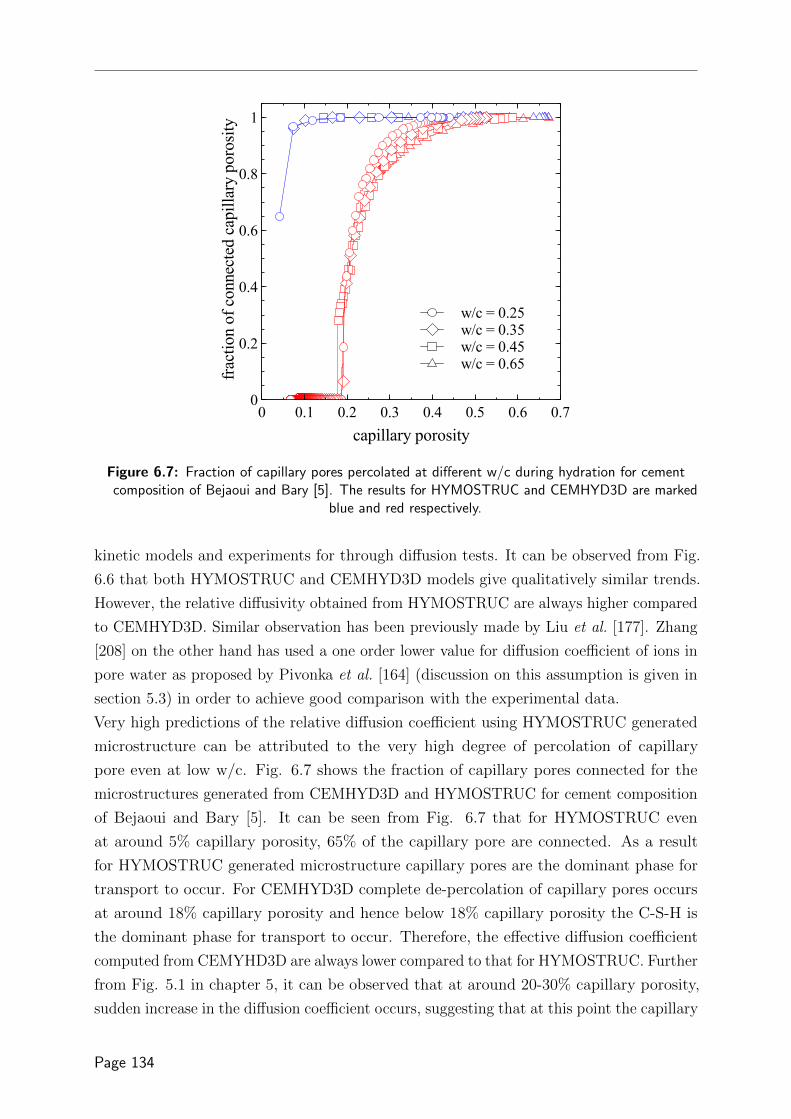
w/c = 0.25w/c = 0.35w/c = 0.45w/c = 0.65

frac

tion

of c

onne

cted

cap

illar

y po

rosit

y

0

0.2

0.4

0.6

0.8

1

capillary porosity0 0.1 0.2 0.3 0.4 0.5 0.6 0.7

Figure 6.7: Fraction of capillary pores percolated at different w/c during hydration for cementcomposition of Bejaoui and Bary [5]. The results for HYMOSTRUC and CEMHYD3D are marked

blue and red respectively.

kinetic models and experiments for through diffusion tests. It can be observed from Fig.

6.6 that both HYMOSTRUC and CEMHYD3D models give qualitatively similar trends.

However, the relative diffusivity obtained from HYMOSTRUC are always higher compared

to CEMHYD3D. Similar observation has been previously made by Liu et al. [177]. Zhang

[208] on the other hand has used a one order lower value for diffusion coefficient of ions in

pore water as proposed by Pivonka et al. [164] (discussion on this assumption is given in

section 5.3) in order to achieve good comparison with the experimental data.

Very high predictions of the relative diffusion coefficient using HYMOSTRUC generated

microstructure can be attributed to the very high degree of percolation of capillary

pore even at low w/c. Fig. 6.7 shows the fraction of capillary pores connected for the

microstructures generated from CEMHYD3D and HYMOSTRUC for cement composition

of Bejaoui and Bary [5]. It can be seen from Fig. 6.7 that for HYMOSTRUC even

at around 5% capillary porosity, 65% of the capillary pore are connected. As a result

for HYMOSTRUC generated microstructure capillary pores are the dominant phase for

transport to occur. For CEMHYD3D complete de-percolation of capillary pores occurs

at around 18% capillary porosity and hence below 18% capillary porosity the C-S-H is

the dominant phase for transport to occur. Therefore, the effective diffusion coefficient

computed from CEMYHD3D are always lower compared to that for HYMOSTRUC. Further

from Fig. 5.1 in chapter 5, it can be observed that at around 20-30% capillary porosity,

sudden increase in the diffusion coefficient occurs, suggesting that at this point the capillary

Page 134

w/c = 0.3w/c = 0.4w/c = 0.5

Sim

ulat

ed (D

e/D0)

10−4

10−3

0.1

1

Experimental (De/D0)10−4 10−3 0.01 0.1 1

Figure 6.8: Comparison between relative diffusivity obtained using microstructures generated fromintegrated kinetic models for electric resistivity experiments of Ma et al. [9]. The predictions fromHYMOSTRUC, CEMHYD3D and CEMYHD3D with only nitrogen accessible pores contributing

to diffusion are marked blue, red and green respectively. Black line represents line of equality.Shaded green region shows factor of 2 bounds and dashed line in red shows factor of 5 bounds.

The area within factor of two bound is represented by shaded region

porosity starts to percolate. This might also be the reason for a good predictions achieved

by CEMHYD3D generated microstructure compared to HYMOSTRUC microstructure for

low to moderate relative diffusivity.

For through diffusion experiments, all the predicted data points (expect one) for HY-

MOSTRUC fall outside the factor of two bounds. For CEMHYD3D around 53% ( of

17 simulated data points) lie within factor of two bounds which is comparable with the

performance of existing analytical models discussed in chapter 5. From Fig. 6.6 it can be

seen that all the data points for low relative diffusivity falls within factor of two bounds for

CEMHYD3D which validates the proposed two scale model with an assumption that only

nitrogen accessible pores contribute to the diffusion of tracers. Furthermore, for higher

relative diffusivity (w/c greater than 0.5), the relative diffusivity is always overestimated

by microstructure models. A possible reason for the over prediction might be higher

contribution from the C-S-H phase. Eq. (6.7) used to estimate the relative fraction of LD

C-S-H is derived empirically for w/c upto 0.5 by Tennis and Jennings [15]. Beyond this

w/c at higher degree of hydration the phase fraction of HD C-S-H according to Eq. (6.7)

would be zero as a result of which C-S-H at that point is assumed to be composed of only

LD C-S-H. This results in very high diffusivity of C-S-H (see Fig. 6.5).

Fig. 6.8 shows the comparison between the relative diffusion coefficient obtained from

Page 135

y=429.36(1/x)

Effe

ctiv

e di

ffusiv

ity o

f chl

orid

e(×

10-1

2 m2 /s)

0

100

200

300

400

500

Effective resistivity(Ω-m)0 5 10 15 20

Figure 6.9: Relationship between the steady stated chloride diffusion coefficient and effectiveresistivity obtained for cement composition of Ma et al. [9].

the microstructures generated from integrated kinetic models and experiments for electric

resistivity measurements of Ma et al. [9]. For the case of electric resistivity good predictions

are observed under the assumption that all gel pores contribute to the measurement. In

case only the nitrogen accessible pores in C-S-H contribute in diffusion the predicted

relative diffusion coefficients are significantly lower than the experimental values as shown

in Fig. 6.8. Thus it can be inferred that differences in measurements observed between

electric resistivity measurements and through/electro migration is due to differences in

contribution of C-S-H with only nitrogen accessible porosity of LD C-S-H allowing transport

of tracers/ions whereas for electric resistivity all C-S-H pores contributes. The relationship

between electric resistivity and chloride diffusivity is often related in literature as [209–211]

De = kCl1

%e(6.11)

where kCl is a fitting factor and %e is the effective resistivity [ML3T−1Q−2]. De in Eq. 6.11

is usually represented in terms of ×10−12 m2/s. The relative diffusivity obtained from the

microstructures for the Ma et al. [9] experiments in case only nitrogen accessible C-S-H

pores contributing to transport can be converted into steady state effective diffusivity of

chloride by multiplying with D0 equal to 2.03× 10−9 m2/s for chloride [212]. Similarly,

relative diffusivity obtained from the microstructures for the Ma et al. [9] experiments in

case all pore contributes can be converted into effective resistivity by multiplying with

the %0 equal to 0.21 Ohm-m, 0.25 Ohm-m and 0.29 Ohm-m for w/c equal to 0.3, 0.4 and

0.5 respectively. %0 being the resistivity of pore water [ML3T−1Q−2]. Fig. 6.9 shows the

Page 136

spheresoblate (c/a = 0.12)prolate (c/a = 10)fibresdisks

Sim

ulat

ed (D

e/D0)

10−5

10−4

10−3

0.01

0.1

Experimental (De/D0)10−5 10−4 10−3 0.01 0.1

Figure 6.10: Comparison between relative diffusion coefficients obtained using microstructuresgenerated from CEMHYD3D and experimental data of Bejaoui and Bary [5] highlighting the

influence of shape of elementary building block of C-S-H.

relationship between electrical resistivity and steady state effective diffusivity of chlorides.

The value of kCl was obtained as 429.36. For concrete the value of kCl as reported by

different authors ranges from 103 to 297 [210, 211] which is lower than that for the cement

paste as fitted for results in Fig. 6.9. This can be attributed to dilution effect in case of

concrete. For instance if the volume fraction of cement paste in concrete is 50% than the

kCl value can be converted to that for concrete by multiplying kCl for cement pate with

paste fraction i.e. 0.5. The kCl for concrete with cement composition of Ma et al. [9] in

this case would be 214.68 (429.36× 0.5) which falls within the range of values as reported

by different authors for concrete.

From Fig. 6.8 it can be inferred that the differences between the predictions from

HYMOSTRUC and CEMHYD3D are lower compared to through diffusion. The possible

reason for this observation is that in case when all gel pores are contributing to diffusion,

the effective diffusivity of the C-S-H is relatively very large compared to C-S-H diffusivity

with only nitrogen accessible pore contributing to diffusion (see Fig. 6.5). Therefore the

effect of de-percolation is less compared to through diffusion experiments. For electric

resistivity measurements, around 80% (of 15 simulated data points) fall within factor

of two bounds for CEMHYD3D generated microstructure showing better performance

compared to existing analytical models discussed in chapter 5.

Fig. 6.10 shows the influence of shape of elementary building block of C-S-H on relative

diffusivity predicted from CEMHYD3D generated microstructure for experimental data of

Bejaoui and Bary [5]. Influence of shape of elementary building block is only noticeable

Page 137

at very low w/c (w/c = 0.25 and 0.3) where the transport essentially occurs through

C-S-H. The estimates of effective diffusivity by different shape (except disks) fall within

the factor of two bounds for these w/c, with spherical shape providing the best estimates.

As discussed in section 6.3, the experimental observations suggest that C-S-H elementary

building blocks do posses an aspect ratio. However, from the perspective of transport the

shape of elementary building block might not be an influential factor.

6.6 Conclusions

The LB scheme presented in part I has been utilized to obtain diffusion coefficient

from microstructures generated from integrated kinetics model. It should be noted that

integrated kinetics models have been developed to obtain correct phase fractions and to

provide microstructures for a given degree of hydration. However, extraction of diffusivity

from these models is a “by product”. For the same capillary pore fraction, these models

can therefore provide different capillary pore connectivity. The C-S-H is treated as a

porous media and its diffusivity is obtained using a two-scale model based on effective

media theory. The effective media theory together with microstructures generated from

integrated kinetics model and lattice Boltzmann scheme thus provides a framework to

explore the influence of different morphological features of cement paste on transport

properties. At present the reduction in diffusivity in gel pores was taken as 1/10 accounting

for constrictivity effects for all type of tracers. However it has been observed that different

ions diffuse differently in cement paste [153, 189] and these differences are associated with

constrictivity. Hence in future a detailed experimental program is needed to accurately

quantify the constrictivity parameter.

A series of simulations were carried out for through diffusion experiments using different

tracers such as HTO, dissolved helium and dissolved oxygen and electric resistivity experi-

ments to have one to one comparison with relative diffusivity obtained from microstructure

generated using two integrated kinetics models viz., HYMOSTRUC and CEMHYD3D. It

was observed that prediction from HYMOSTRUC was higher compared to CEMHYD3D

especially for low relative diffusivity (i.e. low w/c and porosity). For higher diffusivities (i.e.

for high w/c and porosity) and when the difference between diffusivity of C-S-H phase and

capillary pores is small (i.e. in case of electric resistivity experiments), differences between

the diffusivites obtained from microstructures generated using these models decreases.

The possible explanation for this difference is the fact that even at porosity as low as

5%, 65% of the capillary pores are connected in case of HYMOSTRUC whereas in case

of CEMHYD3D a complete de-percolation is noticed. Hence, at low w/c ratio in case of

HYMOSTRUC capillary pores are dominant phase whereas for CEMHYD3D C-S-H is the

dominant phase for transport to occur.

It should be noted that for microstructures generated from integrated kinetic models

Page 138

percolation thershold is a function of resolution and degree of percolation increases with

higher resolution [160, 162]. However, for diffusivity the curcial factor is the capillary

porosity when depercolation occurs as at that point C-S-H phase becomes dominant.

Experimental results show transition at around 17% of capillary pores. Therefore, the

diffusivites predicted from CEMHYD3D generated models shows better co-relation with

experimental data. Around 53% ( of 17 simulated data points) and 80% ( of 15 simulated

data points) of predicted data points from microstructures generated from CEMHYD3D

for through diffusion experiments and electric resistivity experiments respectively falls

within factor of two bounds. The presented approach thus outperforms majority of the

existing analytical models. Further, the results simulated for low relative diffusivity (low

w/c or porosity) were within factor of two bounds indicating good predictive capability

of the presented C-S-H diffusivity model. Simulations were also carried out to access the

influence of the shape of the elementary building blocks on estimated relative diffusivity.

It was observed that differences are only visible at very low w/c (i.e. w/c = 0.25 and

0.3). However, in general the shape of elementary building block does not have a major

influence on predicted diffusivity.

The simulations further reveal that for the tracers such as HTO, dissolved helium and

dissolved oxygen, transport occurs only through nitrogen accessible gel pores whereas

for electric resistivity measurements all gel pores contributes. This in turn provides an

explanation for higher relative diffusivity measured by electric resistivity experiments

compared to the through diffusion technique. It was demonstrated that this can be

further utilized to establish relationship between steady state chloride diffusivity and

electric resistivity experiments. The question now arises whether this explanation is viable.

Jennings [21] suggested that the nitrogen accessible pores represents the large gel pores

of size 3-12 nm whereas the nitrogen inaccessible pores represents small gel pores of size

1-3 nm. The water in the small gel pores is physically bound (also known as “hindered

water” or “constrained water”) and has different physical properties compared to the bulk

pore water. Hence, small gel pores might provide higher resistance to diffusion of tracers

such as HTO, dissolved helium and dissolved oxygen and therefore do not contribute to

transport. On other hand, due to high pH of pore water of cement paste the small gel

pores should be rich in ions which in turn allows to transmit electric current through small

gel pores. Hence even though the small gel pores do not contribute to diffusion of tracers

it might contribute to the electric resistivity measurements. Alternatively, it can also be

the case that the constrictivity in small gel pores is much higher compared to that in large

gel pores. This hypothesis needs to be further explored by taking into account different

constrictivities for LD C-S-H and HD C-S-H. It should be noted that in this case too the

diffusivity of C-S-H should be in the range of the one predicted by the model presented in

absence of contribution from small gel pores as for this values of diffusion coefficient good

agreement is found with the experiments.

Page 139

CHAPTER 7

Leaching of cement paste: mechanisms, influence on properties

and existing modelling approaches

7.1 Introduction

Leaching is a process in which ions get dissolved from the solid phases of cement based

materials and are transported by concentration gradients (diffusion) or/and pressure

gradients (convection). The leaching of calcium ions is of most importance compared to

other leachable ions as calcium based solid phase forms the majority of solid volume in

cement based materials. Therefore, leaching is the term commonly used to refer to calcium

leaching in cement based materials. Hence in this thesis leaching refers to calcium leaching.

Leaching causes dissolution of solid phases such as portlandite and aluminate phases and

causes incongruent dissolution of C-S-H phase. This results in a more porous material

with lower strength and higher permeability and diffusivity. Progression of leaching in

cement based material is very slow (up to a few millimeters in hundred years [17, 18]).

Hence for civil concrete structures with life span of few decades leaching is not considered

an important deterioration mechanism. However, for structures which are in constant

contact with water such as dams, foundations of offshore structures and bridges, water

tanks, sewer pipes, subsurface nuclear waste disposal facility, leaching can be an important

deterioration mechanism and should be taken into account for the service life evaluation

of such structures.

The first half of this chapter provides a overview on current understanding of mechanisms

of leaching, its influence on properties and microstructure of cement paste. The latter

half of this chapter provides overview on the existing modelling approaches for leaching.

Only opc is considered in this review. Section 7.2 gives a general overview on physical

Page 141

and chemical mechanisms. The experimental observations on influence of leaching on pore

structure and properties of concrete are presented in section 7.3. Section 7.4.1 gives an

overview on modeling approaches at continuum scale. The modelling approaches resolving

the microstructure of cement paste are presented in section 7.4.2.

7.2 Chemical and physical mechanisms

Leaching is triggered when cement based materials come in contact with low pH or low

alkaline solution. The pH of pore water in OPC paste lies in the range of around 12.5-13

after hydration. Therefore, any solution with pH below this range (e.g. water) will initiate

leaching and is considered as an aggressive solution. Due to the slow progression of leaching

different techniques have been proposed to accelerate leaching some of which involves the

use of aggressive solutions such as deionized water [13, 14, 213–215], ammonium nitrate

solution [8, 14, 216–227] and ammonium chloride solution [228]. Amongst all, deionized

water and ammonium nitrate are the most commonly used solutions. Leaching rate due to

ammonium nitrate is much faster than deionized water and results in similar end products

(i.e. removal of calcium hydroxide and decalcification of C-S-H) [14, 229]. Ammonium

nitrate reacts with the cement minerals to form calcium nitrate which is highly soluble

and nitro aluminate of calcium which is not very soluble. Calcium nitrate quickly dissolves

in water forming ammonia (which escapes from the system) and releases hydronium ions.

This decreases the pH of solution which accelerates the successive dissolution of calcium

bearing phases. This inturn increases the calcium equilibrium concentration on the onset

of portlandite dissolution from 21 mol/m3 to around 2730 mol/m3 [229]. Alternatively,

the leaching process has also been accelerated in some studies using electric field [230, 231]

or application of a pressurized flow[232].

As the diffusion process is slower in cement paste, the reactions during leaching are usually

equilibrium based. The equilibrium between solid and liquid calcium content can be

described in terms of solid-liquid equilibrium curve (or simply equilibrium curve) as shown

in Fig. 7.1. Fig. 7.1(a) shows the equilibrium curve for leaching caused by deionized water.

This curve marks three distinct stages as explained in [10, 157, 233]. The dissolution of

portlandite occurs in cement paste once alkali such as Na and K are leached reducing

pH of cement paste. The concentration of Ca is maintained at around 21 mol/m3 due to

dissolution of portlandite. On full dissolution the calcium to silica ratio (Ca/Si) in solid is

around 1.65 to 1.8. At this stage incongruent dissolution of C-S-H is initiated. A dissolution

of ettringite and AFm phases also occurs in that zone. The calcium concentration in

liquid at the end of this stage is around 2 mol/m3 and Ca/Si in solid reaches to 1. Further

leaching leads to complete decalcification of C-S-H, transforming C-S-H into an amorphous

silica gel. At this stage the amount of silica in liquid can be as high as 6 mol/m3.

Jacques et al. [234] have noted a large variability in the reported experimental data for

Page 142

Figure

7.1:

Evo

luti

onof

rati

oof

solid

calc

ium

tosi

lica

con

ten

tas

afu

nct

ion

ofca

lciu

mco

nce

ntr

atio

nin

the

liqu

id(e

qu

ilibr

ium

curv

e)(a

)dei

oniz

edw

ater

asp

ub

lish

edby

Bu

ilet

al.

[10]

.T

he

po

ints

ind

icat

esth

eex

per

imen

tal

dat

aco

mp

iled

byB

ern

er[1

1]an

dso

lidlin

eis

fit

toth

ed

ata.

(b)

Am

mo

niu

mn

itra

teas

pu

blis

hed

byW

anet

al.

[12]

.P

oin

tsin

dic

ate

the

exp

erim

enta

ld

ata

and

solid

line

isfi

tto

the

dat

a.

Page 143

Table 7.1: Leaching kinetics parameter for ordinary portland cement paste as reported in literature

reference leaching solution w/c temperature(C)

a(mm/day0.5)

Bellego et al. [216] deionized water 0.4 - 0.12deionized water 0.25 - 0.084deionized water 0.45 - 0.288

Galle et al. [223] ammonium nitrate 0.45 23 174Kamali et al. [14] deionized water 0.25 26 0.075

deionized water 0.4 26 0.14deionized water 0.5 26 0.169deionized water 0.25 85 0.206deionized water 0.4 85 0.328deionized water 0.5 85 0.384ammonium nitrate 0.25 20 1.17ammonium nitrate 0.4 20 1.56

Yang et al. [228] ammonium chloride 0.30 - 0.35

equilibrium curve as reported by different researchers for leaching due to deionized water.

The large experimental variability is observed in the data especially for Ca when 1.25

< Ca/Si < 1.75 and for Si for when Ca/Si > 1.25. Less variability is present for the

maximum Ca concentration (large Ca/Si) and pH. Several authors have listed different

reasons for the variability in the experimental data, including the C-S-H synthesis process,

reaction time and pathway followed to reach equilibrium amongst other things [219, 235].

As a consequence variability is observed between different reactions models of C-S-H for

Ca when 1.25 < Ca/Si < 1.75 [234].

Wan et al. [12] determined the equilibrium curve for leaching under 6 M ammonium

nitrate solution as shown in Fig. 7.1(b). It was found that leaching under 6 M ammonium

nitrate occurs in three stages similar to that of water. The concentration of Ca in liquid is

maintained at around 2950 mol/m3 due to portlandite dissolution. On complete dissolution

of portlandite the Ca/Si in solid is around 1.3 mol/m3 and incongruent dissolution of

C-S-H and dissolution of ettringite and AFm phase is initiated. The calcium concentration

in liquid at the end of this stage is around 130 mol/m3 and Ca/Si in solid is around 0.5.

The values of Ca/Si at the end of stage one and two were observed to be lower than the

typical values reported for leaching by deionized water.

Progression of the leaching front is governed by transport and is diffusion controlled (in

absence of advection) as confirmed by many experimental studies [8, 13, 14, 216, 223, 236].

Therefore leaching depth at a given time can be expressed as

Lx = a√t (7.1)

where, Lx is the leaching depth [L] and a [L1 T−1/2] is the leaching kinetics parameter. The

popular approach to measure degraded depth is to use phenolphthalein. Phenolphthalein

Page 144

turns from colourless in acidic solutions to pink in basic solutions with the transition

occurring at pH around 9.5. However it should be noted that the leaching depth measured

by phenolphthalein does not represent total leaching depth. The total leaching depth being

defined as the distance at which the calcium in solid is the same as that for a reference

unleached material. Bellego et al. [216] based on complementary microprobe analysis

suggested that the degradation depth measured by phenolphthalein should be corrected

by a factor of 1.16 to obtain total leaching depth. Table 7.1 shows the compiled data for

leaching kinetics parameter of OPC paste. Higher w/c leads typically to higher leaching

rate because of a higher porosity. Higher temperature also promotes leaching for both

deionized water and ammonium nitrate. Leaching kinetic parameter in an ammonium

nitrate solution is observed to be around 10 times higher compared to leaching in deionized

water. Poyet et al. [237] have observed that the rate of leaching is sensitive to the frequency

of renewal of leaching solution during test. In test setup where solution is not renewed

the leaching rates observed are lower than that where solution is constantly renewed.

Kamali et al. [238] has proposed a more general relationship to evaluate leaching depth as

a function of time which accounts for a wide range of factors such a water-binder ratio

(w/b), silica fume (SF ), pH, temperature (T ) and experimental protocol (prot). Their

relationship can be expressed as follows

Lx = a× t1/n (7.2)

The leaching depth Lx is expressed in mm, time in days. The parameter n is 2 in absence

of electric field and 1 in presence of electric field. The leaching kinetics parameter was

expressed as

a = a1 × F (w/b)× F (SF )× F (pH)× F (T )× F (prot) (7.3)

a1 is a constant and F (x) represents independent functions taking into account the influence

of water-binder ratio (w/b), silica fume (SF ), pH, temperature (T ) and experimental

protocol (prot). All these functions have been determined by Kamali et al. [238] from

their experimental results.

7.3 Changes in solid phase composition, pore struc-

ture and properties

As presented in the previous section, dissolution of different mineral phases occurs in several

stages. This leads to formation of several distinct altered zones in a degraded sample such as

a fully degraded zone with highly decalcified C-S-H gel at the surface, zone with a partially

degraded C-S-H and fully dissolved ettringite and AFm phases, zone with fully dissolved

Page 145

portlandite and a sound zone [213]. The progression of this zones is linear with square-root

of time [213]. Faucon et al. [214] observed that the mineral composition of the surface

in contact to the deionized water after leaching consisted of residual anhydrates, small

quantity of hydrogarnet dissolved by leaching, iron substituted C-S-H, and magnesium

precipitates in the form of hydrotalcite. The formation of hydrotalcite and ion substituted

C-S-H was attributed to the change in pore water at the surface which increases influx

of iron and magnesium from inner core. Partial leaching of silicon from C-S-H was also

observed near the surface giving evidence of partial dissolution of C-S-H. Precipitation

of ettringite has also been observed in some studies in the zones where portlandite has

completely dissolved [13, 17, 239]. Scanning electron microscope (SEM) and X-ray imaging

results by Phung [8] reveals the presence of portlandite in the transition zone between

fully leached zone and the intact zone as shown in Fig. 7.2. The Ca/Si of solid phase

drops gradually from sound zone to the leached surface as confirmed by X-ray diffraction

[8], X-ray spectroscopy[240], tomography [240] and microprobe analysis [217, 239, 241].

The sample mass decrease is observed due to solid phase alteration during the leaching

[8, 13]. A linear relationship exists between the mass loss due to leaching and square root

of time similar to that for degradation depth [8, 217]. Decrease in mass subsequently leads

to increase in surface area. Phung [8] observed that increase in surface area due to leaching

was around 7 to 15 times and around 4 to 5 times for low and high water-binder ratio

respectively. Such a high increase in surface area indicates the contribution of C-S-H in

increase in surface area. Change in surface area of C-S-H due to decalcification has been

studied in [222, 242]. An increase in surface area is observed on decalcification of C-S-H

from Ca/Si of 1.7 to 1 using both small angle neutron scattering (SANS) and nitrogen

sorption (BET). Further decalcification leads to decrease in surface area. The surface area

measured by SANS is usually higher than the BET surface area. This result suggests that

decalcification transforms the high density C-S-H into a structure with higher specific

surface area i.e. low density C-S-H. The results from SANS reveals that the globule like

morphology is transformed into a sheet like morphology due to decalcification.

Decalcification of C-S-H also induces irreversible shrinkage strains. A marked increase in

shrinkage has been observed when the Ca/Si of C-S-H decreased below 1.2 which could

be attributed to the changes in structure of C-S-H [220]. Chen et al. [220] based on

their experimental investigation has postulated three mechanisms causing decalcification

shrinkage

I A polymerization-induced shrinkage can result if a siloxane bond, induced by the

removal of inter layer Ca in C-S-H, bridges two adjacent regions or surfaces of C-S-H.

Moreover, the enhanced mobility of C-S-H at these low Ca/Si (see mechanism II,

below) facilitates the slight rotations necessary to align the silicate chains of C-S-H

on adjacent surfaces before forming a siloxane bridge.

Page 146

Figure 7.2: SEM image of transition zone of leached sample CH = portlandite, C = residual cementclinkers (top); element (Si, Ca, Al, Fe) mapping generated by X-ray imaging (bottom) (adapted

from from [8])

Page 147

Figure 7.3: Pore size distribution of the initial sample and that leached for 91 days [13].

II The loss of cohesion and subsequent increased mobility of induced shrinkage by

encouraging the structural reorganization of C-S-H into dense morphologies, such as

a progressively layered sheet-like morphology

III At extensive levels of decalcification (i.e., below Ca/Si 0.66), decomposition of the

CaO sheets of C-S-H generates significant shrinkage due to the precipitation and

subsequent polymerization of silica gel.

Both porosity and pore size distribution are significantly altered after leaching. Phung [8]

observed significant increase in number of pores with sizes between 60 nm to 500 nm and

those with pore size less than 10 nm after leaching for cement paste. The increase in pore

volume between 60 nm to 500 nm can be attributed to portlandite dissolution whereas

increase in pore volume less than 10 nm is due to decalcification of C-S-H. Also, Bossa

et al. [243] observed an increase in the volume of pores with sizes between 130 nm to 3.62

µm by a factor 3 using nano and micro tomography. Irrespective of w/c the pore size

distribution is skewed towards larger pore sizes after leaching as shown in figure 7.3. The

porosity of the fully leached zone in cement paste has been found to be around 60-80%

as reported in several studies [157, 243, 244]. Similar to variation of Ca/Si, a gradient of

increasing porosity is observed from sound zone towards degraded zone [8, 244].

Increase in both permeability and diffusivity is evident as leaching induces increase in

porosity. Revertegat et al. [245] reported an increase in diffusivity by a factor 2 and 5 for

tritium and cesium respectively after 30% decalcification. Phung [8] observed that the

increase in permeability was much higher compared to that of diffusivity due to leaching.

Page 148

For the same sample after 28 days of leaching in ammonium nitrate solution the diffusivity

of helium gas increased by 4 times whereas increase in permeability was 25 times. Galle

et al. [223] have reported an increase in permeability by two orders of magnitude for fully

leached (depleted from portlandite) cement paste.

Leaching causes loss of apparent stiffness, a decrease of maximal load (yield stress), and

a decrease of fracture energy [216, 226, 246]. The triaxial behaviour of degraded cement

paste is characterized by an overall strength loss, a loss of frictional performance and a high

sensitivity to drained and undrained conditions [247]. Constantinides and Ulm [248] based

on nano-indentation results suggested that the volumetric fraction of high and low density

C-S-H remains unchanged during leaching. However low density C-S-H undergoes higher

degradation compared to the high density C-S-H with decrease in stiffness of 41% for the

former and 14% for the latter. Leached paste can undergo large plastic deformations which

suggests the C-S-H with a low Ca/Si is highly plastically deformable [249]. Deformations

at failure under tension also increases due to leaching [250]. Heukamp et al. [250] based

on these results stated that the chemical damage of C-S-H matrix dominates over the

increase in macroporosity and in the overall loss of stiffness. Carde et al. [251] on other

hand observed that loss of strength due to the decalcification of C-S-H is only 6% and can

be neglected in relation to the global loss of strength due to the dissolution of calcium

hydroxide.

7.4 Modelling approaches

In this section existing modelling approaches are discussed. The models which do not

resolve the microstructure of cement paste i.e. continuum models are reviewed in section

7.4.1 and models which explicitly resolve microstructure are presented in section 7.4.2

7.4.1 Continuum models

As leaching is a coupled transport and chemical reaction (reactive transport) phenomenon

most models aim to simulate these processes. Many model found in literature consider

only the mass conservation of aqueous calcium under saturated, isothermal condition

[10, 13, 157, 227, 252–256]. This approach has been subsequently extended to account

for advective flow in isothermal conditions [257] and non isothermal conditions [258] and

coupled chemo mechanical effects during leaching [253, 259].The mass conservation of

aqueous calcium can be written as

∂φCCa∂t

= ~∇ ·De~∇CCa −

∂CsCa

∂t(7.4)

Page 149

where CCa is the aqueous Ca concentration, CsCa is the solid Ca concentration, De is the

effective diffusion coefficient of calcium in cement paste and φ is the porosity. CCa can be

linked to CsCa using the equilibrium curves as shown in Fig. 7.1 and therefore

∂CsCa∂t

can be

further expressed in terms of CCa as

∂CsCa

∂t=∂Cs

Ca

∂CCa

∂CCa∂t

(7.5)

Different approaches have been proposed to describe chemical equilibrium under accelerated

conditions in an ammonium nitrate solution. Gerard et al. [260] suggested to use the

equilibrium curve for deionized water but to increase the diffusion coefficient 60 times to

account for acceleration due to 6M ammonium nitrate solution. In references [10, 227, 229]

an equilibrium curve for ammonium nitrate has been used. Phung [8] proposed to

gradually adapt the equilibrium curve from one representative for deionized water to one

representative for a high ammonium nitrate solution in order to account for influence of

spatial-temporal variation of NO3 concentration on chemical equilibrium.

Models coupling thermodynamics with multi-component transport are an alternative to

simulate leaching [156, 261, 262]. The changes in calcium content in solid are obtained

by solving the chemical equilibrium between the mineral and the ionic species in pore

solution. One class of models (multi-component) attribute the same diffusion coefficient

to all aqueous species; consequently electro-kinetic effects induced by a species-dependent

diffusion coefficient are not accounted for [156, 262]. On the other hand, Maltais et al. [261]

have considered electro-kinetic effects by solving Nernst-Planck equation for transport.

Whereas only transport equations for so-called primary species have to be solved for the

former, a transport equation is needed for each aqueous species in the latter making it

computationally expensive. For leaching, Maltais et al. [261] have considered following

8 aqueous species to be transported: K+, Na+, Mg2+, Ca2+, SO2−4 ,OH−, Al(OH)−4 and

Cl−. Stora et al. [262] further coupled the multi-component reactive transport model to a

mechanical model to account for coupled chemo-mechanical effects during leaching. One of

the main factors contributing to uncertainty in modelling leaching with a thermodynamic

approach is the dissolution model for C-S-H [234]. During the last decades, several C-S-H

dissolution models have been proposed with different thermodynamic representation of

C-S-H. The detailed review on these models has been presented in [263, 264]. The selection

of a single C-S-H dissolution model is not straightforward because of the large variability

in experimental solubility data and the fact that all the models seem to reproduce the

experimental data within this experimental variability [234, 263].

An important aspect in modelling leaching is to account for reaction-induced changes

in porosity and diffusion coefficients. For thermodynamics based modeling approaches

changes in porosity are directly determined from the changes in mineral composition

during leaching and molar volumes. However, for simplified models accounting only for Ca

Page 150

transport different approaches have been utilized. Empirical relationship between porosity

and CsCa derived from experiments is used in references [157, 252, 265]. In references

[10, 13, 227, 254] both portlandite and C-S-H are leached out in the form of portlandite

and porosity change is therefore described as

φ = φ0 + V CHm

[CsCa,0 − Cs

Ca

](7.6)

where V CHm is the molar volume of portlandite, φ0 is the initial porosity and Cs

Ca,0 is the

initial Ca concentration. Phung [8] used Eq. 7.6 to obtain change in porosity due to

dissolution for portlandite. The porosity change caused by decalcification of C-S-H in his

model was obtained using a linear relationship between molar volume and calcium in solid

of C-S-H as proposed by Morandeau et al. [266]. This relationship is given as follows

φCSH = φCSH,0 + 0.04CCSH

(1− [Ca/Si]CSH

[Ca/Si]CSH,0

)(7.7)

where φCSH,0 is initial porosity of C-S-H, CCSH is the concentration of C-S-H phase and

[Ca/Si]CSH is Ca/Si of C-S-H and [Ca/Si]CSH,0 is the initial Ca/Si of C-S-H. During

leaching the concentration of C-S-H is assumed to be constant by Phung [8] and the

increase in porosity is accounted by the decrease in molar volume due to change in Ca/Si

of C-S-H.

Different types of empirical relationships have been used to account for change in diffusivity

due to leaching. Empirical relationships such as exponential relationship and modified

Archie’s relationship have been used in [157, 267] and Lee et al. [156] respectively. The

fitting parameters for these relationships have been derived from unleached cement paste

data. Haga et al. [13] proposed an Archie’s relationship type of model as given below

De =

(φ

φ0

)nDe,0 (7.8)

where φ is the porosity and De,0 is the effective diffusion coefficient of the unleached

cement paste. The coefficient n was fitted as 2 based on inverse analysis to match the solid

calcium concentration computed from the model and experiments. Delagrave et al. [268]

proposed the following form of empirical relationship to update diffusivity due to leaching

De = De,0

(Dleache

De,0

)βφCH+αφdφCH+φs

(7.9)

with

α = 1 + (1− β)φCHφs

where Dleache is the effective diffusion coefficient of a fully leached sample, φCH is the

Page 151

fraction of portlandite in the cement paste, φd is the volume fraction of hydrates other

than portlandite, φs is the volume fraction of the hydrates calculated by subtracting the

volume occupied by the portlandite and SiO2 fractions from the total volume of hydrates

in a fully hydrated cement paste. β is the fitting parameter. Gerard et al. [260] suggested

the values of Dleache as 0.4×10−9m2/s and β as 1.3 for w/c ratio of 0.25 and 2.4 for w/c of

0.4.

Analytical relationships for diffusivity based on effective media theory proposed for sound

paste has been extended/utilized to account for change in diffusivity due to change in

porosity. Perko et al. [264] used the relationship proposed by Oh and Jang [146] (See

chapter 5) which is based on generalized effective media theory. Bejaoui and Bary [5]

further extended their series/parallel model (See section 5.3) to apply to leaching. They

assumed an Archie’s relationship type of model to account for changes in diffusivity of low

density and high density C-S-H (which is input parameter in their model) due to increase

in porosity. Similarly, Stora et al. [262] extended multi-coated sphere assemblage model

(See section 5.3) to account for leaching. The changes in the diffusivity of low and high

density C-S-H were accounted for in their model using following relationship

if Ca/Si > 0.8, De,i =

(1− Ca/Si− 0.8

1.65− 0.8

)Dleache,i +

(Ca/Si− 0.8

1.65− 0.8

)De,0,i (7.10)

if Ca/Si ≤ 0.8, De,i = De,0,i

i ∈ LD C-S-H, HD C-S-H

Diffusivity relationships derived from numerical models have also been proposed for

leaching. Marchand et al. [241] used the microstructure generated using CEMHYD3D to

study the influence of the degree of portlandite leaching from cement paste on diffusivity.

Based on their analysis, they proposed a relationship between diffusivity and degree of

portlandite leaching from cement paste as follows

De(φCHleach)−De(φ

CHleach = 0)

De(φCHleach = 100)−De(φCHleach = 0)=

1.1φCHleach2

0.28 + 0.79φCHleach(7.11)

where φCHleach is the fraction of portlandite leached and De(φCHleach) represents effective

diffusivity when the volume fraction of portlandite leached is φCHleach. The De(φCHleach = 100)

required for this model was derived from the microstructure generated from CEMHYD3D.

De(φCHleach = 0) was obtained from same model after converting portlandite voxels in fluid

voxel.

Snyder and Clifton [269] adapted the NIST relationship (see chapter 5) for unleached

cement paste to account for leaching as follows

De(φleach)

D0

= 2DNISTR (φleach)−DNIST

R (φ) (7.12)

Page 152

where φleach is the porosity of leached material, and DNISTR is the relative diffusivity as

computed with the NIST model for unleached cement paste (see section 5.3). van Eijk

and Brouwers [270] used this model to simulate diffusivity changes during leaching with

additional modifications. They used a percolation threshold for leached material of 0.16

compared to 0.18 in sound material. The second modification was to increase contribution

of C-S-H to diffusivity (the third term in NIST model) from 0.001 (for unleached cement

paste) to 0.0025 (which is the relative diffusivity assigned to C-S-H phase while obtaining

diffusion coefficient from CEMHYD3D microstructure [271]). However, this term represents

the contribution of C-S-H which also account for connectivity of C-S-H in the cement

paste microstructures and hence should be smaller than 0.0025. The final form the model

of van Eijk and Brouwers [270] can be expressed as

DeD0

= 0.0025− 0.07φ2 − 1.8H(φ− 0.18)(φ− 0.18)2 + 0.14φ2leach + 3.6H(φleach − 0.16)(φleach − 0.16)2

(7.13)

It should be noted that equation 7.12 has been derived considered leaching of only

portlandite phase and henceforth equation 7.13 does not account for C-S-H leaching. This

relationship has been used by Wan et al. [227] and Phung [8] to model leaching. To account

for the contribution of C-S-H leaching on the diffusion coefficient, Phung [8] considered

that 50% of the volume change in C-S-H during leaching contributes to the capillary

porosity.

7.4.2 Models to simulate leaching through microstructure

Several attempts have been made to explicitly simulate the changes in microstructure

during leaching. Bentz and Garboczi [271] studied the influence of calcium hydroxide

leaching on transport properties. They first simulated the microstructure of hydrated

cement paste using CEMHYD3D. The leaching process is then modelled as a random

dissolution process. For each leaching cycle, the three dimensional microstructure is

scanned to identify all voxels of portlandite which are in contact with pore space. For each

of these voxels, a one-step random walk to one of their six neighbouring sites is executed.

If the step lands in a pore space voxel, that voxel is converted to pore space. Their

study showed that the percolation threshold due to leaching reduced to 16% from 18% for

hydration. This in turn led to higher increase in diffusivity while leaching compared to

decrease in diffusivity during the formation of hydration product. Thus showing that the

diffusivity porosity relationship during leaching do not follow same curve as one during

hydration (a hysteresis behaviour). The modified NIST model for diffusion proposed by van

Eijk and Brouwers [270] discussed in previous section tries to account for this observation

by changing percolation threshold for leached paste from 18% to 16%.

Feng et al. [272] carried out a similar study with the microstructures generated from

THAMES hydration model [273]. This model links microstructure evolution to the

Page 153

thermodynamic equilibrium model GEMIPM2K. Similar to CEMHYD3D, microstructure

evolution during hydration in this model is based on stochastic rules. This model improves

the approach to dissolve and precipitate mineral phases. The probability of dissolution or

precipitation of a voxel is further based on a predefined tendency for a phase to adopt

particular morphologies to achieve realistic crystal shape. The leaching in the approach of

Feng et al. [272] was simulated as a batch reaction using GEMIPM2K thermodynamic

model [121]. By flushing small amounts of pore solution at a given time step, the dissolved

volume fractions of solid phases are computed using the thermodynamic model. Their

approach accounts for changes in microstructure due to dissolution of portlandite, aluminate

and C-S-H phases compared to dissolution of only portlandite phase in the approach of

Bentz and Garboczi [271].Their simulation results revealed very little hysteresis behaviour

between hydration and leaching in contrast to the study of Bentz and Garboczi [271].

They attributed the differences between the two models to the different stochastic rules

used to generate initial microstructures. They also computed the transport and mechanical

properties of the leached microstructure using finite difference and finite element methods

respectively. The change in diffusion coefficient of C-S-H phase and mechanical properties

of C-S-H due to leaching were not taken into account while estimating transport and

mechanical properties. They observed that a sudden change in slope is observed for the

plot of diffusion coefficient with respect to porosity once portlandite is dissolved. Similar

change in the slope is also observed for the plot of elastic modulus with respect to porosity.

The porosity at which the change in slope occurs depends on the w/c. They also observed

that the slope of plot of stiffness with respect to porosity was much stiffer than hydration.

This was due to the loss of portlandite which is much stiffer than C-S-H.

Moranville and co-authors [224, 274] proposed an approach to simulate the changes in

microstructure due to leaching in which they considered a continuum the three dimensional

domain is discretized into 100 µm3 volume elements. The continuum reactive transport

equations are solved along this domain. Transport of ions is solved using the finite volume

method whereas the reaction terms are computed using PHREEQC. The changes in the

diffusion coefficient due to leaching in the transport model is accounted using NIST model

for unleached cement paste. Each of the discritized volume element of the continuum

domain is either associated with boundary fluid or cement paste microstructure generated

using CEMHYD3D. The microstructure is updated during leaching by randomly removing

phases that are in contact with pore fluid to match the dissolved volume fraction.

Bernard and Kamali-Bernard [275] proposed a multiscale approach to determine the

mechanical and transport properties of leached cement paste. They assumed that leaching

progresses in three distinct unleached zone, zone without portlandite and zone without

portlandite and aluminate phases. The thickness of each zone is determined through

empirical relationships obtained through experiments. The transport and mechanical

properties of each zone is determined directly from their microstructure. The initial

Page 154

microstructures of hydrated cement paste were obtained using CEMHYD3D. The leached

microstructures from each zone were determined by turning the dissolved phases into

pore spaces. Their numerical results showed that the complete leaching of portlandite

decreases the compressive strength of a w/c = 0.4 cement paste by a factor of 1.33. The

complete dissolution of portlandite and aluminate phases leads to decrease in compressive

strength by factor of 1.86. Complete leaching of portlandite leads to an increase in diffusion

coefficient by around 30 times. The dissolution of portlandite and aluminate phases leads

to an increase in diffusion coefficient by two orders of magnitude

The models presented above do not simulate the ion transport in the microstructure.

Leaching in those models is carried out by uniformly dissolving the phases in the entire

microstructure to get the required volume fractions. Recently, Gaitero et al. [276] and

Ukrainczyk and Koenders [277] presented models which simulate leaching considering ion

transport in the resolved microstructure. Gaitero et al. [276] presented a pore-scale reactive

transport model for leaching due to ammonium nitrate. The initial microstructure for a

fully hydrated cement paste in their model was generated with HYMOSTRUC. The solid

phases considered in their simulations were, clinkers inner-product C-S-H, outer product

C-S-H and overlapping C-S-H. For describing C-S-H reaction, they assumed that C-S-H

consist of leachable portlandite and non-leachable C-S-H with Ca/Si equal to one. Hence

the reaction due to leaching in their model is represented solely in terms of portlandites

dissolution. Gaitero et al. [276] accounted for the increase in diffusivity of C-S-H phase

due to dissolution through a linear relationship with respect to porosity. The transport

equation (in their case Nernst-Planck equation) was solved using a finite element method.

Ukrainczyk and Koenders [277] similarly used the HYMOSTRUC model to generate intial

microstructure and considered only C-S-H dissolution in presence of deionized water using

an equilibrium curve similar to one shown in Fig. 7.1. The diffusivity of C-S-H was

evolved in their model as a function of Ca/Si in solid phase. A linear interpolation was

carried out between the known points. They considered following known points: Ca/Si

1.7, 1, 0, the assumed diffusion coefficients were D0/200, D0/3 and D0 respectively. The

transport equation (diffusion equation) was solved using implicit finite difference scheme

and diffusion of only calcium ions was considered.

7.5 Conclusions

An overview on experimental observations on leaching mechanisms, its influence on mi-

crostructure and properties of opc paste and existing modeling approaches not resolving

microstructure (continuum approaches) and ones resolving microstructure has been pre-

sented. Leaching due to its slow progression is usually studied experimentally under

accelerated conditions. The two most commonly used leaching solutions are ammonium

nitrate and deionized water. For both solution equilibrium curve shows three distinct parts

Page 155

viz., marking complete dissolution of portlandite, start of decalcification of C-S-H and

dissolution of aluminate phases and complete dissolution of aluminate phases and further

decalcification of of C-S-H phases. The progression of the leaching front for both aggressive

solutions is diffusion controlled. However, the kinetic rate parameter for leaching under

ammonium nitrate solution is ten times higher than that for deionized water.

Leaching leads to formation of zones in the altered material. The outer most zone contains

highly decalcified iron substituted C-S-H surface with residual unhydrated cement particles,

hydrogarnet (only small quantity dissolved) and hydrotalcite; the zone with fully leached

portlandite and the zone next to the unleached cement paste which might contain small

amount of portlandite. Decalcification leads to increase in surface area, decrease in the

bulk density and results in shrinkage due to decalcification of C-S-H. C-S-H undergoes

structural changes due to decalcification and based on SANS data different researchers

have concluded that C-S-H morphology is transformed from globule like morphology into

sheet like morphology.

Leaching causes an increase in porosity and the pore size distribution is skewed towards

higher pores. Leaching causes an increase in permeability and diffusion coefficient and a

loss of stiffness. The nano-indentation tests on leached C-S-H reveals that the low density

C-S-H undergoes higher degradation than high density C-S-H. However the volume fraction

of both high density and low density C-S-H was observed to be constant.

At continuum scale, simplified reactive transport models accounting for only mass transport

of Ca and multi-component transport models coupled with thermodynamic models have

been used to simulate leaching. The porosity change due to leaching in case of simplified

model is computed either through empirical relationships or considering C-S-H reaction

in terms of portlandite. Different types of relationships have been used to account for

changes in diffusion coefficient due to leaching. All these relationships have some form of

fitting parameters which need to be determined. For some relationships these parameters

have been determined from the experimental data of unleached cement paste. For others

these parameters have been determined by comparison with experimental and predicted

leaching profiles. However, due to the lack of experimental data on changes on diffusion

coefficient due to leaching it is difficult to access the predictability of these models.

Models explicitly resolving the microstructure and simulating changes in microstructure

due to leaching have been developed. Two types of approaches exist in literature. In

a first approach, the dissolution of different phases is carried out by dissolving mineral

phase in contact with pore water in a stochastic way. Such an approach leads to a

uniform microstructure rather than different zones that are observed during leaching.

The alternative approach is to use a coupled reactive transport framework to simulate

leaching through microstructure. Two models have been proposed recently which only

account for dissolution of C-S-H in microstructure. The changes in diffusion coefficient of

C-S-H due to change in porosity in these models have been accounted for through simple

Page 156

empirical relationships. There is still a lack of a robust model to simulate changes in

microstructure during leaching. Such a model will not only pave a way forward towards

a multi-scale framework, but also serve as an important tool to understand changes in

material properties during leaching for which very little experimental data exist.

Page 157

CHAPTER 8

Modelling changes in microstructure of cement paste under

calcium leaching

8.1 Introduction

Modeling of reactive transport processes using a transport model coupled with geochemical

solver is computationally expensive. For instance, solving the benchmark on C-S-H

dissolution as presented in section 4.5.3 takes around 2 days using a desktop computer

with 3 GHz Intel Xenon processor. Hence in order to simulate reactive transport processes

for a three dimensional microstructure for a longer duration of leaching it is essential

to develop an alternate approach. In this chapter, a simplified reactive transport model

which is deduced from a geochemical model has been developed. This model considers

transport of only Ca and Si components. The reactions are implemented as look-up tables

which have been pre-computed with the geochemical solver PHREEQC thus eliminating

a need of invoking the geochemical model at each time step. The equivalence of the

simplified model to coupled reactive transport model has been established through a set

of benchmarks. Further the two-scale model for C-S-H diffusivity as proposed in Chapter

6 has been extended to account for changes in C-S-H structure during leaching. Finally

the simulations of leaching are carried out on the microstructures generated from both

CEMHYD3D and HYMOSTRUC. Section 8.2 details the simplified modeling approach

developed for leaching. Finally the results of the simulation for calcium leaching on

microstructures generated from CEMHYD3D and HYMOSTRUC are presented in section

8.3.

Page 159

8.2 Simplified reactive transport model for leaching

and its implementation

The flow chart for the approach to simulate calcium leaching through the microstructure

of the cement paste is presented in Fig. 8.1. The transport of Ca and Si components are

described using the advection-diffusion-reaction equation under similar assumptions as

discussed in Section 4.1. The advection-diffusion-reaction equation is solved using the

TRT LB scheme for multilevel porous media with a D2Q5 lattice and a linear EDF as

described in section 3.2.2 with an additional source/sink term as explained in section 4.3.

For the reactive transport problem (with explicit coupling), the time step should respect

the Neumann criteria in order to ensure reliable solutions (as discussed in chapter 4).

However, this results in a very small time steps. For instance, for the benchmark on C-S-H

dissolution as presented in section 4.5.3 the time step is kept around 3 µs to respect the

Neumann criteria. This makes it computationally expensive to simulate leaching during

the longer time span. To overcome this limitation, an adaptive relaxation scheme was

used which is inspired from the PID (proportional, integral, differential) adaptive time

stepping scheme used for conventional numerical methods [278–282]. The adaptation of

PID scheme in terms of relaxation parameters for LB method is described in appendix

I. This approach allows to safely increase the relaxation time and in turn the time step,

while keeping the errors below certain tolerance value.

The molecular diffusion coefficient for both Ca and Si is taken as 2.2×10−9m2/s [157]. The

diffusion coefficient in capillary pores Dp is equal to the molecular diffusion in water (D0)

and porosity φ is equal to one. Only portlandite, clinkers and C-S-H phase are explicitly

represented in microstructure for reasons of simplicity. In case of CEMHYD3D, hydration

products other than portlandite and C-S-H are also represented as C-S-H. Portlandite

and clinker phases are non-diffusive whereas the effective diffusion coefficient De for the

C-S-H phase is computed using the two-scale diffusion model as described in section 6.3.

In this model, the C-S-H is assumed to be composed of HD C-S-H as an inclusion in the

matrix of LD C-S-H. Input parameters for this model are the volume fractions of pores

and solids in LD C-S-H and HD C-S-H. The approach to compute these volume fractions

for initial microstructure has been described in section 6.4. During leaching, solid and

pore fractions of HD C-S-H and LD C-S-H have to be updated. Using the updated phase

fractions, the diffusion coefficient is updated using the two-scale diffusion model. The

approach to update the volume fraction of solid and pore space in LD and HD C-S-H

due to dissolution is presented in section 8.2.1. Due to the lack of experimental data

on the influence of constricitivity on ion transport in gel pores, the diffusivity of ions in

gel pores is assumed to a order of magnitude lower than molecular diffusion coefficient

in pure water (see also chapter 6). When Ca/Si in C-S-H becomes less than one, the

constrictivity effects are neglected and the diffusivity in the gel pores is taken as the

Page 160

Generate

microstructures

Integrated kinetic models (HYMOSTRUC, CEMHYD3D)

Input parameters Bogue’s composition, water-cement

ratio, Blaine's fineness

Hydrate till required degree of

hydration is achieved

HYMOSTRUC CEMHYD3D

streaming step

Apply domain boundary conditions

Apply portlandite reaction boundary

condition

Collision step

Compute source/sink term for C-S-H

reaction

Update solid phase boundary due to

portlandite dissolution

Update C-S-H porosity and diffusion

coefficient

Update relaxation parameters

required

time

achieved

Simplified Leaching model

PID controller to compute new

maximum relaxation time in domain

no

yes

Leached state

Figure 8.1: Overall approach to simulate leaching through hardened cement paste microstructuresgenerated using integrated kinetics models

Page 161

(a)C C

aeq,CSH

(mM

)

0.00

5.00

10.00

15.00

20.00

Ca/Si0.8 1 1.2 1.4 1.6

(b)

C Sieq,CSH

(mM

)

0

0.5

1

1.25

Ca/Si0.8 1 1.2 1.4 1.6

(c)

V CSH

(cm

3 /mol

)

5557.5

6062.5

6567.5

70

Ca/Si0.8 1 1.2 1.4 1.6

(d)

N CSH

(t)/N

CSH (t

=0)

0

0.2

0.4

0.6

0.8

1

Ca/Si0.8 1 1.2 1.4 1.6

Figure 8.2: Relationships between Ca/Si in C-S-H and (a) Equilibrium Ca concentration (b)Equilibrium Si concentration (c) Molar volume (d) ratio of moles of C-S-H to initial moles of

C-S-H

molecular diffusion coefficient in the water. This assumption is justified by the fact that

C-S-H starts to undergo drastic structural changes at Ca/Si below one,which is observed

in both experiments (see discussion section 7.3) and in thermodynamic model (see Fig

8.2 (d) where at Ca/Si below one the sudden decrease in number of moles is seen). As a

result at this point it can be assumed that the pores in C-S-H are large enough to neglect

constrictivity effect.

As mentioned previously, leaching of only portlandite and C-S-H due to deionized water

is considered presently and other minor mineral phases such as ettringite and aluminate

phases in case of CEMHYD3D generated microstructures which also undergoes dissolution

are treated as C-S-H phase. The dissolution reactions for C-S-H and portlandite are

considered through equilibrium chemistry as the leaching is diffusion controlled process

(see discussion in chapter 7). Dissolution reaction of C-S-H results in the additional

source/sink term for Ca and Si transport equation at the volume element where C-S-H is

Page 162

present. This source/sink term is computed as follows

RCahom,CSH = φ

(Ceq,CSHCa − CCa)

∆t, RSi

hom,CSH = φ(Ceq,CSH

Si − CSi)∆t

(8.1)

where RCahom,CSH and RSi

hom,CSH are homogeneous source/sink term of Ca and Si components

respectively due to C-S-H dissolution [N1L−3T−1]. CCa and CSi are the aqueous concen-

tration of Ca and Si components [N1L−3]. φ is the porosity and ∆t is the time step [T]

which is one for LB scheme. Ceq,CSHCa and Ceq,CSH

Si are the equilibrium concentrations for

Ca and respectively which depend on Ca/Si in the solid of C-S-H phase as described later.

As C-S-H undergoes incongruent dissolution the change in porosity due to dissolution is

preliminarily due to the change in the molar volume which is given as

φCSH =NCSH

V(VCSH(~r, t+ ∆t)− VCSH(~r, t)), ~r ∈ ΩCSH (8.2)

where V is the volume of the element, ΩCSH represents the C-S-H domain, φCSH is the

porosity of the C-S-H, VCSH is the molar volume [N−1L3] and NCSH is the moles of C-S-H

phase [N]. NCSH during the initial stage of C-S-H (Ca/Si > 1) dissolution does not vary

significantly. However, during later stage NCSH can vary (see Fig. 8.2). The dissolution of

portlandite is a heterogeneous reaction and at the boundary of the portlandite, following

condition is applied

Cca|Γ=Γport = Ceq,portCa (8.3)

where Γport represents the boundary of the portlandite, Ceq,portCa is the equilibrium concen-

tration for Ca component. This boundary condition is implemented using the approach

described in section 4.2. The change in geometry due to dissolution is carried out using

the approach given in section 4.4. The molar volume of portlandite phase is taken as 33

cm3/mol.

The relationships for equilibrium concentrations, change in molar volumes and change in

moles as a function of Ca/Si in solids for C-S-H and the equilibrium concentration for

portlandite were determined using flush-type geochemical simulations 1 using PHREEQC.

The thermodynamic database CEMDATA07 [126, 283–285] was used to obtain the relevant

thermodynamic constants. C-S-H phase in the geochemical reaction model is represented

as an ideal solid solution using the CSHQ solid solution model proposed by Kulik [131].

The CSHQ solid solution model is more consistent in terms of reproducing the solubility

curves and it gives a more realistic prediction of C-S-H gel densities and volume changes

compared to two phase solid solution model as proposed by Kulik and Kersten [286] which

is part of CEMDATA07. From the geochemical model, the equilibrium concentration for

1A flush-type reaction path simulation calculates equilibrium between aqueous and solid phase duringdifferent steps (or water-cycles). After each step, an increment of unreacted fluid is added to the systemdisplacing the existing fluid and leaving the reacted minerals in place. Such a type of simulation is alsocalled a mixing-flow reaction in chemical engineering

Page 163

Transport model coupled with geochemical solverSimplified model

24 mM NaOH

43 mM NaOH

8 mM NaOH

Avg.

con

c in

dom

ain

(M)

0

0.0025

0.005

0.0075

0.01

0.0125

0.015

0.0175

Time (s)0 10 20 30 40 50 60

(a)

length (microns)

wid

th(m

icro

ns)

60 70 80 9060

70

80

90

43 mM NaOH

24 mM NaOH

8 mM NaOH

(b)

Figure 8.3: Portlandite dissolution benchmark: (a) evolution of average Ca concentration inaqueous phase. (b) Final shape of grain at the end of 60 s. Dotted line represents simplified

model and solid lines represents the model coupled with geochemcial solver.

Page 164

portlandite (Ceq,portCa ) is ∼19.48 mM for leaching under deionized water. The relationships

for equilibrium concentrations, change in molar volumes and change in moles as a function

of Ca/Si in solids for C-S-H for leaching under deionized water are shown in Fig. 8.2.

Experimental data show that there exist an unique relationship between Ca/Si and the

parameters such as equilibrium concentrations and change in molar volumes [233, 266] which

was also confirmed by simulating flush-type reactions with different initial concentrations

of CaO and SiO2. These relationships are implemented in the simplified model as a

look-up table and a second order Lagrange polynomial is used for interpolation between

the tabulated values. When the C-S-H voxel is in contact with portlandite, portlandite is

dissolved first in order to equilibrate the aqueous Ca concentration. This can be simply

implemented by applying the portlandite boundary condition before the collision step

of LB scheme as shown in Fig. 8.1. This simplified approach can thus be viewed as

a scheme in which the chemical reactions (state) are precomputed and tabulated thus

eliminating the need to solve the complex geochemical system which in turn increases the

computational efficiency.

To validate the proposed approach for portlandite reaction, the example on portlandite

dissolution as presented in section 4.6.1 was used. In this example dissolution of a fictional

portlandite grain is carried out at different pH values which are obtained by introducing

different NaOH concentrations. The equilibrium Ca concentration for portlandite for 8

mM, 24 mM and 43 mM NaOH solutions used in this example were found to be 16.89

mM, 12.53 mM and 8.818 mM respectively. Fig. 8.3 shows the comparison between the

results using the transport model coupled with the geochemical model and the simplified

approach presented in this section. Good agreement is observed between both models thus

validating the portlandite dissolution model for leaching.

To validate the model for C-S-H dissolution, the example presented in section 4.5.3 was

simulated using the simplified model. Using the simplified model, this example takes

around 15 minutes using a desktop computer with 3 GHz Intel Xenon processor. The

comparison between the transport model coupled with the geochemical model for reaction

and the simplified model are shown in Fig. 8.5. Fig. 8.4 shows the change in relaxation

parameter carried out through PID scheme during this simulation. Good agreement is

observed between the two approaches. It is also of interest to compare the results obtained

with a simplified model considering only the transport of Ca component, as it is commonly

used approach for simulating leaching [10, 157, 260, 264]. In this model further, the change

in number of moles of C-S-H due to leaching is not accounted for (i.e. relationship Fig.

8.2 not used). Fig. 8.6 shows that in case of only Ca transport, good agreement is not

observed between Ca in solid and liquid phase at inlet of the domain where considerable

leaching has occurred.

Page 165

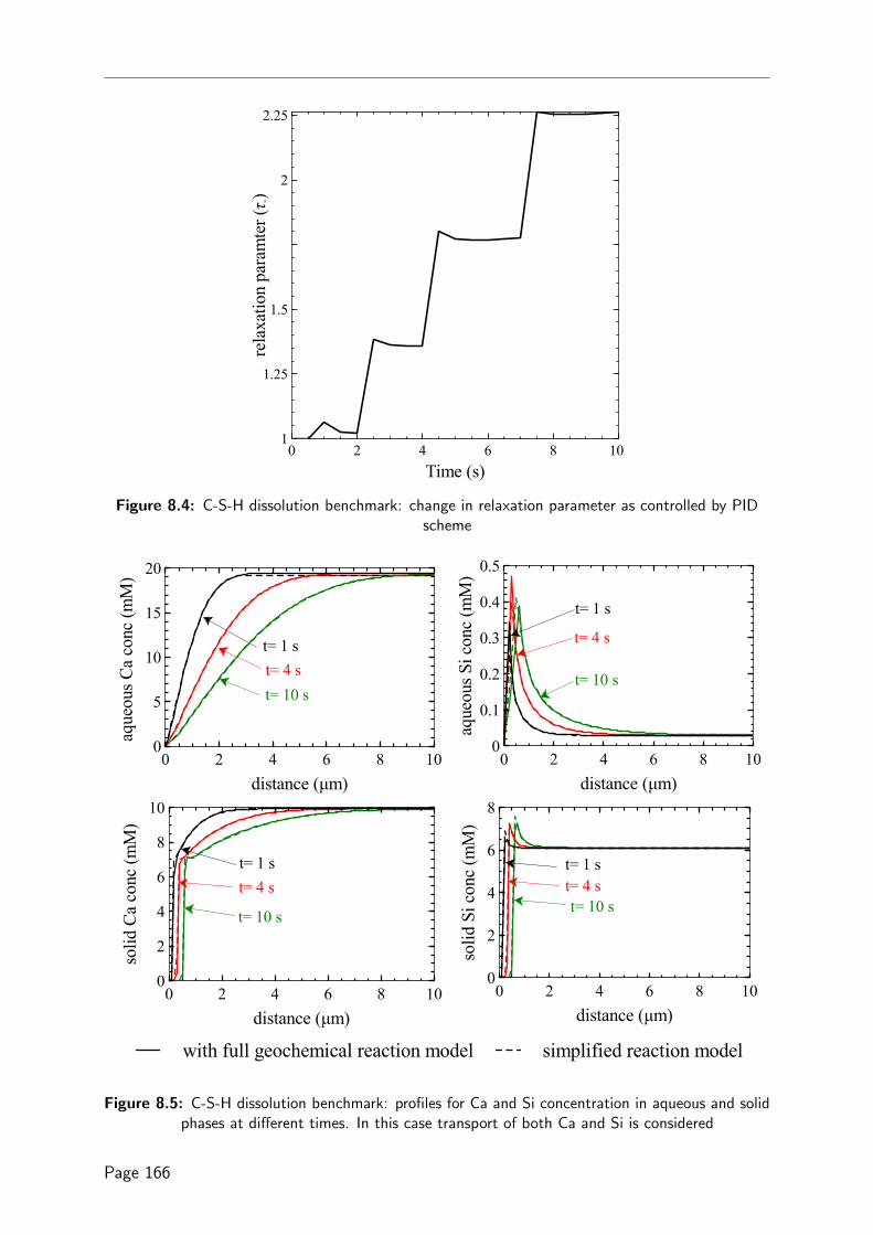
rela

xatio

n pa

ram

ter (τ -)

1

1.25

1.5

2

2.25

Time (s)0 2 4 6 8 10

Figure 8.4: C-S-H dissolution benchmark: change in relaxation parameter as controlled by PIDscheme

aque

ous C

a co

nc (m

M)

0

5

10

15

20

t= 10 st= 4 st= 1 s


t= 10 s

t= 4 s

t= 1 s

aque

ous S

i con

c (m

M)

0

0.1

0.2

0.3

0.4

0.5


t= 10 s

t= 4 st= 1 s

solid

Ca

conc

(mM

)

0

2

4

6

8

10


t= 1 s

with full geochemical reaction model simplified reaction model

t= 10 st= 4 s

solid

Si c

onc

(mM

)

0

2

4

6

8


Figure 8.5: C-S-H dissolution benchmark: profiles for Ca and Si concentration in aqueous and solidphases at different times. In this case transport of both Ca and Si is considered

Page 166

aque

ous C

a co

nc (m

M)

0

5

10

15

20

t= 10 st= 4 st= 1 s


t= 10 st= 4 st= 1 s

simplified reaction modelwith full geochemical reaction model

solid

Ca

conc

(M)

0

10


Figure 8.6: C-S-H dissolution benchmark: profiles for Ca concentration in aqueous and solid phasesat different times. In this case transport of only Ca considered

8.2.1 Updating of volume fractions due to leaching

As a result of dissolution the C-S-H, an additional pore space is created as a result of

which volume fractions of solids in LD C-S-H and HD C-S-H and pore fraction of LD

C-S-H and HD C-S-H need to be updated which are inputs for the two-scale C-S-H model

presented in section 6.3. To update these volume fractions, additional assumptions are

made

I The fractions of HD C-S-H and LD C-S-H remain unchanged during leaching. Based

on nano-indentation test, Constantinides and Ulm [287] have shown that during

leaching the volume fractions of HD C-S-H and LD C-S-H remain unchanged.

II The degradation rate of LD C-S-H is different from HD C-S-H. More specifically, LD

C-S-H degrades faster than HD C-S-H [287]. Constantinides and Ulm [287] reported

an elastic modulus of LD C-S-H and HD C-S-H as 21.7± 2.2GPa and 29.4± 2.4GPa

for sound paste and 3.0± 0.8GPa and 12.0± 1.2GPa respectively for leached paste.

The residual values of elastic modulus thus being 41% and 14% for LD C-S-H and

HD C-S-H respectively of the initial ones.

III The ratio of change in porosity of LD C-S-H and HD C-S-H remains constant during

leaching.∆φLDp∆φHDp

= RHDLD (8.4)

RHDLD denotes the relative change in LD C-S-H porosity with respect to HD C-S-H

porosity. Further, by definition the ratio of change in solid fractions of LD C-S-H

and HD C-S-H(

∆φLDs∆φHDs

)is also equal to RHD

LD . Assuming that a linear relationship

Page 167

exists between porosity and elastic modulus as suggested in refs. [196, 288], RHDLD

can be determined as

RHDLD ≈

∆ELD∆EHD

≈ 21.7− 3.0

29.4− 12.0≈ 1.075 (8.5)

ELD and EHD being the elastic modulus of LD C-S-H and HD C-S-H respectively.

This assumption can be verified by carrying out nano-indentation tests on C-S-H

with different Ca/Si and if found wrong, should be suitability modified.

The change in the fractions of solids of LD C-S-H and HD C-S-H phases in a C-S-H volume

can then be determined as

∆φCSHs,HD =

(∆φCSHs

φCSHHD +RHDLD φ

CSHLD

)φCSHHD (8.6)

∆φCSHs,LD = ∆φCSHs −∆φCSHs,HD

Correspondingly the volume fraction of solids of LD C-S-H and HD C-S-H in C-S-H volume

can be determined as φCSHs,LD + ∆φCSHs,LD and φCSHs,HD + ∆φCSHs,HD respectively. The fractions of

pores in HD C-S-H and LD C-S-H can be determined as

φCSHp,HD = φCSHHD − φCSHs,HD, φCSHp,LD = φCSHLD − φCSHs,LD (8.7)

The porosity of HD C-S-H and LD C-S-H and nitrogen accessible porosity in LD C-S-H

can finally be determined as

φHDp =φCSHp,HD

φCSHHD

, φLDp =φCSHp,LD

φCSHLD

, φLDnit =φCSHp − 2φCSHp,HD

φCSHLD

(8.8)

8.3 Results and Discussions

Simulations of leaching due to deionized water were carried out on the microstructures

generated from HYMOSTRUC and CEMHYD3D for OPC with composition used by

Kamali et al. [14] (Bogue’s composition: 73.4%, 10.3%, 3.9% and 5.8% for C3S, C2S,

C3A, C4AF respectively) who carried out leaching experiments with deionized water.

Simulations were carried out for two different w/c viz., 0.25 and 0.4. The size of the

generated microstructure was taken as 65 µm × 65 µm × 65 µm which is smaller than

the REV (100 µm × 100 µm × 100 µm) used for diffusion computations, however it still

represents a reasonable size2. The microstructures generated were hydrated for up to 3

months (similar to curing time used in experiments) before subjecting to leaching. To

simulate leaching, a additional layer of nodes which represent the leaching fluid is added to

2Similar size has been determine has been determined as REV for Hain et al. [186]. See section 5.5 ondiscussion on REV.

Page 168

left side of the simulation domain. The concentration of both Ca and Si at this boundary

are set to zero to represent deionized water. All other boundaries are set as zero flux

boundaries. Simulations were carried out for 800 s.

Fig. 8.7 shows the evolution of average Ca in the aqueous phase, solid phase, C-S-H

and portlandite content with time. As expected, the cement paste with w/c equal to 0.4

undergoes faster leaching because of its higher initial diffusivity and capillary porosity

compared to cement paste with w/c equal to 0.25. Fig. 8.7 also shows that irrespective of

the integrated kinetic model or w/c, the relative (with respect to initial content) amount

of protlandite dissolved is much more compared to the amount of Ca leached from C-S-H.

Hence leaching of portlandite is often considered more significant in some models and

is also commonly observed in experiments (see chapter 7). Further from Fig. 8.7, it

can be clearly seen that the microstructure generated from HYMOSTRUC undergoes

higher leaching compared to CEMHYD3D. This is due to the fact that HYMOSTRUC

generated microstructures exhibits lower percolation threshold for capillary pores compared

to CEMHYD3D (as discussed in section 6.5).

Fig. 8.8 shows the profiles of average Ca concentration in solid phase, C-S-H and portlandite

content at the end of 800 s. Leaching clearly leads to the formation of distinct zones

viz., intact zone (where no leaching has occurred), transition zone (where portlandite is

partially dissolved) and zone where portlandite is completely dissolved and C-S-H has

considerably dissolved. Fig. 8.8 further shows that in the transition zone, the leaching of

C-S-H is also initiated. The presence of portlandite and partially leached C-S-H has been

found experimentally through SEM images by Phung [8] (see Fig. 7.2). In a well-mixed

system at thermodynamic equilibrium, C-S-H leaching only initiates after the portlandite

is completely dissolved. However in the cement paste microstructure, portlandite grains

can also be embedded in the C-S-H matrix and C-S-H can leach first. Hence the presence

of portlandite and partial leaching of C-S-H is plausible in the transition zone due to the

morphological characteristics of cement paste. Fig. 8.8 also shows that the transition zone

is much wider for w/c equal to 0.25 than 0.4 irrespective of the integrated kinetic models

use to generate microstructure. For w/c of 0.25 the transition zone is found from around 0

µm to 30 µm for CEMHYD3D and around 5 µm to 40 µm for HYMOSTRUC. For w/c of

0.4 the transition zone ranges from around 30 µm to 45 µm for CEMHYD3D and 30 µm

to 50 µm for HYMOSTRUC.

Fig. 8.9 shows the porosities profiles at 800 s. From Fig. 8.9 and Fig. 8.8 it can be inferred

that, for w/c of 0.25, alterations in microstructure has occurred upto 30 µm and 40 µm

for CEMHYD3D and HYMOSTRUC respectively. Similarly for w/c of 0.4, alterations in

microstructure has occurred upto 45 µm and 50 µm for CEMHYD3D and HYMOSTRUC

respectively. From the leaching kinetic parameters determined by Kamali et al. [14] (as

summarized in table 7.1) the depth of the leaching front can be determined as 7.2 µm

and 13.45 µm for w/c of 0.25 and 0.4 respectively after 800 s. The leaching depth in the

Page 169

(a)C ca(t)/C

ca(t=0)

0.7

0.8

0.9

1

time (s)0 200 400 600800

(b)

w/c =0.25 (CEMHYD3D)w/c =0.4 (CEMHYD3D)

w/c =0.25 (HYMOSTRUC)w/c =0.4 (HYMOSTRUC)

C cas(t)

/Ccas(t=0)

0.7

0.8

0.9

1

time (s)0 200 400 600 800

(c)

C caCSH(t)

/CcaCSH(t=0)

0.850.880.900.930.950.981.00

time (s)0 200 400 600800

(d)C caport (t)/C caport (t=0)

0.40.50.60.70.80.9

1

time (s)0 200 400 600 800

Figure 8.7: Evolution of (a) average total calcium concentration in aqueous phase (b) average totalcalcium concentration in solid phase (c) average calcium concentration in C-S-H phase (d)

average portlandite content over time.

Page 170

C caCS

H(t)

/CcaCS

H(t=

0)

00.20.40.60.8

1

distance (μm)0 10 20 30 40 50 6070

C capo

rt (t)/C

caport (t=

0)0

0.20.40.60.8

1

distance (μm)0 10 20 30 40 50 60 70

w/c = 0.25 (CEMHYD3D)w/c = 0.4 (CEMHYD3D)w/c = 0.25 (HYMOSTRUC)w/c = 0.4 (CEMHYD3D)

(d)C cas(t)

/Ccas

(t=0)

00.20.40.60.8

1

distance (μm)0 10 20 30 40 50 6070

Figure 8.8: Profiles of (a) average Ca concentration in C-S-H phase (b) average portlandite content(c) average Ca concentration in solid phase at the end of 800 s. Average is taken over the plane

perpendicular to direction of leaching.

Page 171

w/c = 0.25 (CEMHYD3D)w/c = 0.25 (HYMOSTRUC)w/c = 0.4 (CEMHYD3D)w/c = 0.4 (HYMOSTRUC)

tota

l por

osity

0.2

0.4

0.8

1

distance (μm)0 10 20 30 40 50 60 70

Figure 8.9: Average total porosity profile at the end of 800 s. Average is taken over the planeperpendicular to direction of leaching.

Figure 8.10: Example of cement paste sample along with corresponding TGA results after leaching(adapted from Kamali et al. [14]).

Page 172

(a)

(b)

Figure 8.11: Three dimensional veiw of Ca front for w/c=0.25. Region in red and blue representsregion with Ca ≥ 19mM and Ca < 19mM respectively. a) CEMHYD3D b) HYMOSTRUC

Page 173

(a)

(b)

Figure 8.12: Three dimensional veiw of Ca front for w/c=0.4. Region in red and blue representsregion with Ca ≥ 19mM and Ca < 19mM respectively. a) CEMHYD3D b) HYMOSTRUC

Page 174

(a) (b)

(c) (d)

Figure 8.13: Ca front for w/c=0.25 CEMHYD3D microstructure. Region in red and blue representsregion with Ca ≥ 19mM and Ca < 19mM respectively. a) back view b) front view c) bottom view

d) top view

Page 175

(a) (b)

(c) (d)

Figure 8.14: Ca front for w/c=0.25 HYMOSTRUC microstructure. Region in red and bluerepresents region with Ca ≥ 19mM and Ca < 19mM respectively. a) back view b) front view c)

bottom view d) top view

Page 176

(a) (b)

(c) (d)

Figure 8.15: Ca front for w/c=0.4 CEMHYD3D microstructure. Region in red and blue representsregion with Ca ≥ 19mM and Ca < 19mM respectively. a) back view b) front view c) bottom view

d) top view

Page 177

(a) (b)

(c) (d)

Figure 8.16: Ca front for w/c=0.4 HYMOSTRUC microstructure. Region in red and bluerepresents region with Ca ≥ 19mM and Ca < 19mM respectively. a) back view b) front view c)

bottom view d) top view

Page 178

work of Kamali et al. [14] was determined visually. Fig 8.10 shows the leached sample

obtained from the experiments of Kamali et al. [14] where the leached zone can be clearly

distinguished from unleached zone. The TGA analysis further supports that the leached

zone does not contain portlandite, thus suggesting that the leaching depth determined

form their experiment corresponds to portlandite dissolution front. The experimental

leaching depth thus closely corresponds to the depth that mark beginning of the transition

zones in the microstructure simulation. From Fig. 8.8 it can be seen that the beginning of

the transition zone is roughly marked at around 0 µm and 3 µm for CEMHYD3D and

HYMOSTRUC respectively for w/c of 0.25 and around 25 µm and 30 µm for CEMHYD3D

and HYMOSTRUC respectively for w/c of 0.4 which is more closer to the experimental

values. This relatively large (compare to the size of the simulation domain) transition

zone observed in simulations might be due to small size of REV used for this simulations.

In future detailed analysis of REV for leaching should be carried out. Fig. 8.11 - Fig.

8.16 shows the leaching fronts which differentiate the zones where the Ca concentration is

aqueous phase < 19 mM and ≥ 19 mM. These figures clearly show that for this size of

REV large undulations are observed in the front.

8.4 Conclusions

In this chapter an efficient model has been developed to simulate leaching through

cement paste microstructure. The efficiency of this simplified model is achieved firstly by

development of a new adaptive relaxation scheme which allows to have larger time steps

while keeping errors within certain bounds and secondly by replacing the geochemical

computations with precomputed relationships implemented in the form of a look up

table. The simplified model only considers transport of two components viz., Ca and Si.

The comparison with the reactive transport model coupled with the geochemical solver

confirms the accuracy of the simplified model. Further it was found that the commonly

used approach, wherein only transport of Ca is considered was unable to capture the

profile in the initial part of the domain where considerable leaching has occurred. Thus

transport of both Ca and Si was found to be essential. The two-scale diffusion model for

C-S-H has been further extended for leaching. Certain heuristic assumptions were to made

to update the volume fractions of pores in LD C-S-H and HD C-S-H onsite of leaching.

Further detailed experimental investigation might be necessary to confirm or modify these

assumptions.

The developed model was used to simulate leaching from the microstructure of OPC paste

with two different w/c viz. 0.25 and 0.4. It was found that the cement paste with the

higher w/c undergoes more leaching. The relative amount (with respect to initial) of

portlandite dissolved is much higher compared to the calcium leached from the to C-S-H

for both w/c. It was further observed that HYMOSTRUC generated microstructures

Page 179

undergoes more leaching compared to CEMHYD3D. This is due to the fact that the

capillary pores percolation threshold for HYMOSTRUC is much lower compared to

CEMYHD3D as a result of which capillary pores are dominant phase for transport in case

of HYMOSTRUC. Formation of distinct zones viz., an unleached intact zone, a trasition

zone where portlandite is partially leached and a zone where portlandite is fully leached

and C-S-H undergoes considerable leaching was observed in the leached microstructures.

In the transition zone portlandite is partially leached and initiation of leaching of C-S-H

is observed. Thus unlike common presumption, the leaching of portlandite and C-S-H

can occur at the same time. Bigger transition zones are observed for lower w/c. The

leaching depth observed (depth till the intact zone) was much larger compared to values

determined from experiments. However, the leaching depth obtained from experiment

closely correspond to depth marking the beginning of transition zone. The reason for

the difference in experimental observation and simulation can be the large width of the

transition zone as a result of which sharp front was not observed in the simulations. This in

turn might be associated with the small size of microstructure used in this study. In future

an REV analysis for leaching should be carried out in order to determine the appropriate

size of REV needed for leaching simulations.

Page 180

CHAPTER 9

Retrospection, Conclusions and Way forward

9.1 Retrospection

As highlighted in the introduction of this thesis, the specific need for this project arose

from the necessity to understand how concrete would age over a very long period of time

in a near surface Belgian nuclear waste disposal system. Due to the large time scale

involved and the slow nature of physio-chemical processes which degrade concrete, it is

extremely difficult to experimentally study the process of ageing. As a result a need for

a computational suite which can simulate the changes in morphology due to ageing was

identified. Indeed the altered morphology generated from this model can be further used

to estimate changes in properties due to ageing and hence such a tool could prove to be a

useful virtual probe to investigate ageing processes.

Based on this view point the specific objectives of this thesis were identified viz., to

develop a numerical framework that is able to simulate changes in morphology due to

physico-chemical processes and to apply this framework to first predict the diffusivity of

cement paste and secondly to simulate the leaching process. The prediction of diffusivity

of cement paste further requires development of the description of C-S-H diffusivity based

on morphological parameters. The prediction of diffusivity with a reasonable accuracy is

essential as it defines the susceptibility of the cement paste to undergo physico-chemical

degradation. It is also regarded as an important parameter in service life prediction of

concrete structures. The leaching process is one of the important detrimental processes to

be considered for the service life assessment of the structures are in contact with water

or can come in contact with water such as ear surface Belgian nuclear waste disposal

system. Further due to its slow nature, very few studies exists on the influence of leaching

on the properties (especially transport properties) of cement paste. Hence the successful

Page 181

demonstration of the ability of the developed framework to simulate leaching can pave

a way forward to develop a comprehensive knowledge on influence of leaching on the

properties of the cement paste.

In order to achieve these goals a lattice Boltzmann (LB) method based framework was

developed in this study. The developed framework can simulate mass transport and reactive

transport processes through the pore-scale and multilevel systems. Specific developments

were made in field of LB methods viz., development of a local second order convergent

generalized boundary condition for advection-diffusion equation, development of a new

PID based relaxation scheme to allow for higher time-step while keeping errors in check

and a new diffusion velocity LB scheme which allows to fix the relaxation parameter to

a value that best suites the stability and accuracy while allowing for variability of both

the time step and spatial heterogeneity of diffusion coefficients. A consistent approach

was developed to link LB schemes with external geochemical solver wherein heterogeneous

reactions are treated as pseudo-homogeneous reactions. This approach allows to account

for heterogeneous reactions and homogeneous reaction in same way which made coupling

of LB scheme with the external geochemical solver PHREEQC possible using sequential

non-iterative approach. The developed framework has been implemented in a newly

developed LB method based multi-physics tool called Yantra.

To achieve the second goal of obtaining reliable prediction of diffusivity of cement paste,

a new two-scale diffusivity model of C-S-H based on effective media theory has been

developed. This model has been further extended to account for leaching. This model

along with the LB framework to simulate mass transport and microstructures generated

from integrated kinetic models presents a tool to explore the role of morphology and pore

spaces in cement paste on diffusivity. Finally in order to simulate leaching, a simplified

model has been developed which considers transport of only Ca and Si components and the

reaction of C-S-H in this model was implemented as a look up table. This approach has the

same level of accuracy as the transport model coupled with the geochemical solver however,

it reduces the computational times from days to minutes. This made the simulation of the

reactive transport processes (resulting in dissolution of portlandite and decalcification of

C-S-H) due to calcium leaching through the microstructure of reasonable size feasible.

9.2 Conclusions

The main conclusions that can be drawn from the work carried out in this thesis are

summarized below —

• LB method provides an efficient numerical framework to simulate mass transport

and reactive transport processes through a pore-scale and multilevel systems. The

voxelized pore structures generated from integrated kinetic models or computed

tomography can be used as an direct input in the LB methods.

Page 182

• The pseudo-homogeneous treatment of heterogeneous reactions, even though slightly

less accurate compared to the conventional approach to treat boundary conditions,

presents an ability to treat both homogeneous and heterogeneous reactions in the

same way thus allowing the use of a single source/sink term. This allows for coupling

of the LB method and an external geochemical solver.

• A series of simple examples highlighting the influence of parameters such as solution

composition, surface area and spatial arrangement of mineral phases on dissolution

of fictitious portlandite grain reveals that, under diffusive transport conditions and a

thermodynamic equilibrium approach, different initial pH conditions do not influence

the overall reaction rate (time needed to reach equilibrium is the same). However,

lower pH values increase the amount of dissolved portlandite resulting in smaller

grains at the end of simulation. Further, spatial arrangement of mineral grains is

more important than the surface area. The spatial arrangement of grains may cause

local equilibrium in certain parts of the domain inhibiting local dissolution processes

at the grain surface.

• From the study of influence of pore network on portlandite dissolution, four cases

consisting of random porous media with same portlandite fraction but differing in

particle sizes or total porosity (by introducing inert material), it was observed that

for diffusion controlled dissolution the tortuosity and the porosity of the porous

media have a more pronounced effect compared to particle size and surface area.

• Using the developed two-scale model for C-S-H diffusivity, the LB scheme and

integrated kinetic models, it is possible to estimate the diffusivity of cement paste

within the uncertainty band defined by the experimental results complied from

literature.

• It was found from the wide range of experimental data complied from literature,

that relative diffusivity measured by electrical resistivity is always higher compared

to through-diffusion techniques (measured using HTO or dissolved gases as tracer).

Using the two-scale model for diffusivity, it was found that this difference is due to

different contribution of gel pores. In case of the tracers such as HTO, dissolved

helium and dissolved oxygen, transport occurs through nitrogen accessible gel pores

(present in LD C-S-H) whereas for electric resistivity measurements all gel pores

contribute resulting in higher measurements for electric resistivity. This observation

can be used in future to establish the link between diffusivity of tracers and electric

resistivity 1.

• The influence of the shape of C-S-H elementary bricks on relative diffusivity is only

visible at very low w/c (i.e. w/c = 0.25 and 0.3). For varities of shapes (except disks)

1Electric resistivity is easy to measure and often used as non-destructive in-situ technique.

Page 183

the predicted values for low w/c lies within factor of 2 bounds. Therefore, it can be

presumed that the shape of C-S-H elementary bricks may not be of importance for

transport properties.

• By comparison between different integrated kinetic models, it was found that the

diffusivity predicted from microstructures generated from HYMOSTRUC (a vector

based hydration model) is always higher compared to that from CEMYHD3D (a voxel

based hydration model). These differences are more pronounced for low to moderate

w/c and diminishes at higher w/c ratios. Further when difference of diffusivity

between C-S-H phase and capillary pores is less (i.e. electric resistivity experiments)

the differences between diffusivity predicted from microstructures generated from

HYMOSTRUC and CEMHYD3D is less. The reason for these differences is due to

the very low percolation threshold for HYMOSTRUC. In case of HYMOSTRUC,

even at porosity as low as 5%, 65% of the capillary pores are connected, whereas in

case of CEMHYD3D a complete depercolation is observed at porosity lower than

18%. Similarly in case of leaching, the microstructure generated from HYMOSTRUC

undergoes more leaching compared to CEMHYD3D.

• Using the simplified model developed for leaching it is possible to simulate the leaching

through microstructures of reasonable size. Qualitatively correct microstructures of

the leached sample can be obtained from the developed model.

• From simulations of leaching carried out on microstructures of cement paste, it was

observed that cement paste with higher w/c undergoes more leaching. The relative

amount (with respect to initial) of portlandite dissolved in much higher compared to

the amount of calcium leached from C-S-H. Further, leaching leads to formation of

distinct zones viz., an intact unleached zone, a transition zone where protlandite is

partially leached and a zone where protlandite is fully leached and C-S-H undergoes

considerable leaching. In the transition zone, the initiation of leaching of C-S-H was

also observed. Thus unlike common presumption, the leaching of portlandite and

C-S-H can occur together at the same time. Bigger transition zones are observed

for lower w/c. The leaching depth observed (depth till the intact zone) was much

larger compared to the values determined from experiments. However, the leaching

depths obtained from experiments closely correspond to depth marking the beginning

of transition zone. The reason for the difference in experimental observation and

simulation can be the large width of the transition zone as a result of which a

sharp front was not observed in the simulations. Further simulations with larger

microstructures can be carried out in future in order to reduce the width of transition

zone (in terms of overall sample size) and to achieve sharp front.

Page 184

9.3 Way forward

In this thesis for the first time (as per the author’s knowledge) the simulation of leaching

through the microstructure of cement paste considering both reaction and transport

processes have been achieved. This in turn is a first step towards the development of

a computational suite that can simulate physico-chemical changes occurring in cement

paste during ageing and the development of multi-scale, multi-physics approach to mimic

the ageing of concrete. In order to further attain this goal following aspects need to be

addressed in future

• The algorithms implemented in Yantra can be also be used to investigate the role of

ITZ in the leaching of mortar and to develop an suitable upscaling framework for

leaching of concrete.

• Changes in microstructure due to other physico-chemical processes such as carbona-

tion, sulphate attack, occurring during the ageing of concrete can be explored with

the developed framework.

• The approach of pre-tabulating geochemical computations provides a lucrative

alternative to transport solver coupled with thermodynamic calculations and can be

further explored for other reaction networks commonly encountered in the ageing of

concrete (such as sulphate attack, carbonation).

• To extend the developed approach to variably saturated porous media. Indeed, in

most cases concrete is under saturated and hence this is an essential extension in

future. Variable saturation is also important to simulate degradation processes such

as carbonation which are often studied in experiments at unsaturated conditions

(60-70% relative humidity).

• For ion transport electro-kinetic effects can be important and hence a transport

solver accounting for electro-kinetic effects (Nerst-Planck equation solver) should be

implemented in future in Yantra and further coupled with PHREEQC.

• The capabilities of Yantra should be further extended to include/couple different

physics such as thermal transport, mechanics (fracture propagation) and water flow.

Depending on the applications, these different physics may play a crucial role in

simulating aging of concrete.

• At present there is very little information on constrictivity of cement paste and

hence experiments focusing on the study of constrictivity parameter are needed to

better predict transport of different ions or tracers. The constrictivity effects can also

be studied by coupling molecular dynamics simulations with single pore transport

simulations (see for instance [289, 290]).

Page 185

• Heurstic assumptions have been made in this thesis with regard to how the phase

fractions of LD C-S-H, HD C-S-H and pores in LD C-S-H and HD C-S-H evolve

during leaching. Further experimental investigation on nano-indentation tests and

BET tests at different Ca/Si ratio of C-S-H can provide more insights into the

changes of these volume fractions (see for instance [15, 248]).

Page 186

A

Yantra: A lattice Boltzmann method based tool for multi-physics

simulations in hetergoenous porous media

The algorithms presented in this thesis have been implemented in a newly developed

lattice Boltzmann method based framework for multi-physics simulation named as Yantra

(in sanskrit it means a tool or a device). The outline of Yantra framework is shown

in Fig. A.1. The object oriented framework of Yantra is implemented in Python with

computationally intensive tasks and LB solvers implemented in FORTRAN. Python also

act as a communicator between two different solvers (e.g. LB solver and PHREEQC ). At

the heart of Yantra lies three main modules preprocessor, physics and postprocessor which

users can use to define their model. The preprocessor module provides two objects mesh2d

and mesh3d which can be used to generate 2d or 3d domain respectively. The the most

important variable in mesh class is the array called nodetype which marks whether the

node is treated as solid or liquid. The nodes with nodetype values less than or equal to zero

are treated as liquid nodes and greater than zero are treated as solid nodes. The nodetype

can take any value and can be used as in indicator to differentiate between different

material types. Further this objects contain specific methods to import microstructures

from integrated kinetic models or to mark simple shapes such as sphere, circle, rectangle

or a box in the nodetype array with a specific indicator value. These objects are initialized

by specifying domain bounds (rectangle in case of 2D and box in case of 3D). The mesh2D

and mesh3D objects are weakly associated to physics.

physics module contain specific kernels to solve certain type of physics. physics module is

further divided into continuum, pore and multilevel referring to solver solving physics at

continuum scale, pore scale or multilevel scale respectively. At present in pore and multilevel

modules their exists two physics implementations viz., transport and reactivetransport.

Page 187

preprocessor physics postprocessor

LB solvers Geochemical

solvers

Solver layer

Fortran/ C++

computationally

intensive

operations

Model

components

python

User defined model

Figure A.1: Outline of Yantra framework

The transport module contains solvers to solve advection-diffusion and diffusion equation

whereas reactivetransport module contain transport solver coupled with phreeqc and

simplified models. The initialization of any object in physics class requires passing

of instance of mesh object, a dictionary data structure for domain parameters and a

dictionary data structure for domain boundary conditions. Default initialization of different

parameters have been implemented for users not familiar with LB schemes and sanity check

on initialization are incorporated to avoid erroneous input. Additional parameter required

to initialize physics object are blocksize and nprocs. The LB solvers are implemented with

a blocking scheme1 to make it cache efficient and blocksize can be used to specify the size

of the block. The implementation of LB solvers includes openMP directives and nprocs

can be used to specify the number of threads (processors) to be used. The collision step

in LB solvers have been further optimized2. The streaming step is implemented using

swap technique to avoid need for two different copies of distribution functions [76]. The

association of mesh object instance to physics object instance can be further exploited

to parallelize a simulation on a multi-core architecture using message passing interface

(MPI). The parallelization of Yantra physics instance using MPI has been demonstrated

but is not included in the current version.

Post-processing of results can be carried out using Matplotlib [291] a python library in

case of 2D plots. For 3d post-processing output can be obtained from Yantra in vtk

format which can be visualized in Paraview [292]. The postprocessor module at present

1The idea of the blocking scheme is to divide data into chunks that can fit the L1 cache.2The collision term is expanded in order to reduce the number of floating point operations

Page 188

Figure A.2: Output of Yantra

contains a plot3d module which is a wrapper written on top of Mayavi2 library [293],

which provides basic three dimensional visualization functionality. Yantra requires only

one time compilation which can be carried out with automatic setup file accompanied

with it. For installation Yantra requires python 2.6 or higher distribution, a FORTRAN

compiler and python packages viz., SciPy and NumPy. This packages can be installed

using a full python installer such as Python (x,y) [294]. All the implementations of Yantra

are accompanied with series of benchmarks. At present around 20 benchmarks are included

with Yantra. To develop a model in Yantra first a mesh instance is created and then a

physics instance is created. The simulation can be ran up to require time using run method

in physics instance. The example code for a simple model to simulate the a diffusion in

3D domain is given below and the output of the code is plotted in Fig. A.2

1 """

2 An example code to create a model in Yantra

3 """

4 import Yantra #imports Yantra

5 #------lets begin with creating instances of this objects--------

6 #mesh instance

7 #50x50x50 domain with 1 as dx

8 m = Yantra.preprocessor.mesh3d(0, 50, 0, 50, 0, 50,1, loc=’nodal’)

9 #physics instance

10 dp =’D’:1./6. #diffusion coefficient taken as 1/6

Page 189

11 bc =’left’:[’conc’ ,1.0],

12 ’right’:[’conc’,0.0],

13 ’top’: [’flux’,0],

14 ’bottom’:[’flux’,0],

15 ’front’: [’flux’,0],

16 ’back’:[’flux’,0],

17 #left and right as concentration boundary and all other are flux boundaries

18 #use SRT D3Q7 LB solver for diffusion equation

19 physics= Yantra.physics.pore.transport.diff.SD3Q7

20 p = physics(m,dp,bc,8) #number of processors taken as 8

21 p.run(tf=5000) #final time for run as 5000

22 #plotting simulation

23 #get x,y,z co-ordinates

24 x,y,z=m.get_coordinates()

25 Yantra.postprocessor.plot3D.contour3d(x,y, z, p.conc ,m.nodetype, m.dx)

Page 190

B

From Boltzmann equation to lattice Boltzmann equation

Lattice Boltzmann method can be derived by discretizing Boltzmann equation in terms of

directional velocity [295, 296]. The Boltzmann equation is given as follows

∂f

∂t+ ~e · ~∇f = Ω (B.1)

where f is the distribution function [NL−3] , ~e is the directional velocity [L1,T−1] and Ω

represents the collision term. Discretizing Boltzmann equation in terms of directional

velocity gives∂fi∂t

+ ~ei · ~∇fi = Ωi, i = 1, 2, ..., q (B.2)

Here q is the number of discrete velocities. Discretizing time using forward finite difference

scheme we get∂fi∂t

=fi(~r, t+ ∆t)− fi(~r, t)

∆t(B.3)

~r is the position vector. substituting Eq. (B.3) in Eq. (B.2) we get,

fi(~r, t+ ∆t)− fi(~r, t)∆t

= −~ei · ~∇fi(~r, t) + Ωi(~r, t) (B.4)

Eq. (B.4) shows that in order to obtain the lattice boltzmann equation from the discrete

boltzmann equation the right hand side has to be subjected to the upwind treatment.

Upwind schemes use an adaptive or solution-sensitive finite difference stencil to numerically

simulate the direction of propagation of information in a flow field. The upwind schemes

attempt to discretize hyperbolic partial differential equations by using differencing biased

in the direction determined by the sign of the characteristic speeds. The upwind scheme is

Page 191

stable if it satisfy the Courant-Friedrichs-Lewy condition

Courant number:e∆t

∆r≤ 1

For conventional lattice Boltzmann implementations e, ∆t and ∆r are usually set to 1

and hence this condition is satisfied. In case of discrete boltzmann equation velocities ~ei

define upwind and downwind directions, a characteristic line is defined by ~ei.The upwind

treatment in the case of discrete boltzmann equation means that RHS term at time t in Eq.

(B.4) is evaluated at ~r−~ei∆t. From there the information travels along characteristic line in

time ∆t and arrive point r. That is ~∇fi(~r, t) = ~∇fi(~r− ~ei∆t, t) and ~Ω(~r, t) = ~Ω(~r− ~ei∆t, t),

fi(~r, t+ ∆t)− fi(~r, t)∆t

= −~ei · ~∇fi(~r − ~ei∆t, t) + Ωi(~r − ~ei∆t, t) (B.5)

replacing ~r with ~r + ~ei∆t we get

fi(~r + ~ei∆t, t+ ∆t)− fi(~r + ~ei∆t, t)

∆t= −~ei · ~∇fi(~r, t) + Ωi(~r, t) (B.6)

using forward difference for the space derivative

~ei · ~∇fi(~r, t) =f(~r + ~ei∆t, t)− fi(~r, t)

∆t(B.7)

substituting Eq. (B.7) in Eq. (B.6) and rearranging we get

fi(~r + ~ei∆t, t+ ∆t) = fi(~r, t) + ∆tΩi(~r, t) (B.8)

Eq. (B.8) represents the general form of the lattice botlzmann equation. If the collision

term is replaced with the BGK term a well known single relaxation time lattice boltzmann

scheme can be obtained from above equation. The BGK collision operator (ΩBGK) is given

as

ΩiBGK(~r, t) = −1

τ(fi(~r, t)− f eqi (~r, t)) (B.9)

and the single relaxation time lattice boltzmann scheme is given as

fi(~r + ~ei∆t, t+ ∆t) = fi(~r, t)−1

τ(fi(~r, t)− f eqi (~r, t)) (B.10)

f eqi is the equilibrium distribution function.

Page 192

C

Equilibrium distribution function in lattice Boltzmann method

Equilibrium distribution function satisfies Maxwell-Boltzmann distribution given as

f eq(~e, C, ~u) = C( m

2πkT

)3/2

exp

(−m(~e− ~u) · (~e− ~u)

2kT

)(C.1)

where m is the particle mass and kT is the product of Boltzmann’s constant and tempera-

ture. Replacing kT/m = e2s/γ we get

f eq(~e, C, ~u) = C

(2πe2s

γ

)−3/2

exp

(−(~e− ~u) · (~e− ~u)

2e2sγ

)(C.2)

es represents the speed of sound and γ is the adiabatic constant. Eq. (C.2) can be

rewritten as

f eq(~e, C, ~u) = Cw(~e)F1(~e, ~u)F2(~u)

w(~e) =

(2πe2s

γ

)−3/2

F1(~e, ~u) = exp

(2~e · ~u2 e

2s

γ

)

F2(~e, ~u) = exp

(−~u · ~u

2 e2s

γ

)(C.3)

Substituting the Taylor series expansion for the exponents in eq. (C.3) we get

exp(x) = 1 + x+x2

2!+x3

3!+ · · · (C.4)

Page 193

and

f eq(~e, C, ~u) = w(~e)C

[1 + γ

~e · ~ue2s

+ γ(~e · ~u)2

2e2s

− γ (~u · ~u)

2e4s

]+O(~u3) (C.5)

In general the above equilibrium distribution function can be written as

f eq(~e, C, ~u) = w(~e)C[A1 + A2(~e · ~u) + A3(~e · ~u)2 + A4(~u · ~u)

]+O(~u3) (C.6)

The unknown coefficients A1, A2, A3, and A4 are determined based on fact that equilibrium

distribution function must satisfy conservation of mass, momentum, energy. The order up

to which terms must be considered in f eq is generally determined by governing equation

intend to be solve. For eg., to arrive to Naiver-Stokes we need terms up to order of ~u2.

However to arrive to advection diffusion equation terms up to order of ~u suffice requirement.

Remark C.0.1 (pseudo lattice speed of sound) For γ = 1 the equilibrium distribu-

tion function given by Eq. (C.5) can be rewritten as

feq(~e, C, ~u) = w(~e)C

[1 +

~e · ~ue2s

+(~e · ~u)2

2e2s

− (~u · ~u)

2e4s

]Using this equilibrium distribution function to recover the Naiver-Stokes equation the rela-

tionship between pressure (P ) and density (ρ) can be recovered as [297]

P = e2sρ

Therefore es is generally referred to as lattice speed of sound. However the term es has no

physical significance for advection-diffusion equation and hence in this thesis es is referred

to as pseudo lattice speed of sound.

Page 194

D

Multiscale Chapman-Enskog expansion

The governing partial differential equation can be recovered from the lattice Boltzmann

equation using the a multiscale Chapman-Enskog expansion. The lattice Boltzmann

equation is given as

fi(~r + ~ei∆t, t+ ∆t) = fi(~r, t) + ∆tΩi(~r, t) (D.1)

Expanding fi(~r + ~ei∆t, t+ ∆t) using taylor series expansion

fi(~r + ~ei∆t, t+ ∆t) = fi(~r, t) +n=∞∑n=1

1

n!

[∆t

(∂

∂t+ ~ei · ~∇

)]nfi(~r, t) (D.2)

Substituting Eq. (D.2) in Eq. (D.1) we get

n=∞∑n=1

1

n!

[∆t

(∂

∂t+ ~ei · ~∇

)]nfi(~r, t) = ∆tΩi(~r, t) (D.3)

Retaining only terms upto second order in Eq. (D.3)[∂

∂t+ ~ei · ~∇+

∆t

2

(∂2

∂t2+ 2

∂

∂t~ei · ~∇+ ~ei~ei : ~∇~∇

)]fi(~r, t) = Ωi(~r, t) +O(∆t3) (D.4)

In Chapman-Enskog expansion space and time derivatives are expanded with respect to a

small perturbation ε. The time derivative is expanded as

∂

∂t= ε

∂

∂t1+ ε2 ∂

∂t2+O(ε3) (D.5)

Page 195

and space derivative is expanded as

~∇ = ε~∇∗ +O(ε2) (D.6)

The distribution function and collision term is likewise expanded starting from zeroth

order.

fi = f(0)i + εf

(1)i + ε2f

(2)i +O(ε3) (D.7)

Ωi = Ω(0)i + εΩ

(1)i + ε2Ω

(2)i +O(ε3) (D.8)

Substituting, Eq. (D.5), Eq. (D.6), Eq. (D.7) and Eq. (D.8) in Eq.(D.4) and neglecting

O(ε3) terms we get

[ε∂

∂t1+ ε2 ∂

∂t2+ ε~ei · ~∇∗ + ε2 ∆t

2

∂2

∂t21+ ε2∆t

∂

∂t1~ei · ~∇∗ + ε2 ∆t

2~ei~ei : ~∇∗~∇∗

](f

(0)i + εf

(1)i

)= Ω

(0)i + εΩ

(1)i + ε2Ω

(2)i (D.9)

Finally grouping the terms to same order the conservation laws at different scales can be

discussed separately.

O(ε0) :Ωi = 0 (D.10)

O(ε1) :

[∂

∂t1+ ~ei · ~∇∗

]f

(0)i = Ω

(1)i (D.11)

O(ε2) :

[∂

∂t2+

∆t

2

∂2

∂t21+ ∆t

∂

∂t1~ei · ~∇∗ +

∆t

2~ei~ei : ~∇∗~∇∗

]f

(0)i +

[∂

∂t1+ ~ei · ~∇∗

]f

(1)i = Ω

(2)i

(D.12)

The macroscopic variables are defined as the moments of the distribution function and the

macroscopic dynamics can be expressed by means of the conservation laws applied to some

of this moments. A global conservation of a macroscopic quantity is expressed locally by a

collision invariant. For example, conservation of mass is enforced by a local conservation

of mass during the collision between particles. At the level of lattice Boltzmann equation

this means that the∑

i Ωi should be zero.

Page 196

E

Quasi stationary assumption for heterogeneous reactions

The change in concentration of jth species in solid (Cj,s) due to heterogeneous reaction

can be written as∂Cj,s

∂t= −Rj

het (E.1)

Rjhet in above equation represents source/sink term in aqueous concentration corresponding

to heterogeneous reaction. Correspondingly the mass balance for aqueous concentration

(Cj) at fluid-solid interface in terms of aqueous concentrations can be written as

∂Cj

∂t= ~∇ · ~J j +Rj

het (E.2)

Only small change in solid concentration is sufficient to greatly affect the solution compo-

sition in liquid phase. As a result at the fluid-solid interface the aqueous solution spends

much of its time in stationary state. This implies that ∂Cj

∂t≈ 0. This is commonly referred

to as quasi-state approximation [110]. As a consequence Eq.(E.2) can be written as

~∇ · ~J j = −Rjhet (E.3)

Taking volume integral over the volume of the solid domain Eq. (E.3) we get∫Vs

~∇ · ~J jdVs =

∫Vs

−RjhetdVs (E.4)

Using Gauss’s divergence theorem we get∫Γs

n · ~J jdΓs =

∫Vs

−RjhetdVs (E.5)

Page 197

Assuming the flux and reaction terms to be constant over the solid surface we get

n · ~J j = − VsAsRjhet (E.6)

where Vs is the volume of the solid and As is the surface area of the solid. Thus the

heterogeneous reactions occurring at the fluid-solid interface can be represented as the

boundary conditions using Eq. (E.6).

Page 198

F

Summary of mathematical expressions for different effective

diffusivity models for cement paste

The mathematical expressions and the fitting parameter involved for the different models

to predict effective diffusivity of cement paste are summarized below :

F.1 Empirical model

Archies relationship

De

D0

= aφn

De is the effective diffusion of cement paste [L2 T−1], D0 is the diffusion in pore water [L2

T−1], φ is capillary porosity

Fitting parameters: a, n

Modified Archie’s relationship

De

D0

= a(φ− φc)n ∀φ > φc

De

D0

= 0 ∀φ ≤ φc

φc is the threshold capillary porosity

Fitting parameters: a, n, φc

Page 199

Exponential form

De

D0

= a exp(nφ)


Exponential form with respect to water-cement ratio

De

D0

= a exp(nw/c)

w/c is the water-cement ratio


F.2 Relationships derived from numerical models

NIST model Garboczi and Bentz [137]

De

D0

= a1H(φ− φc)(φ− φc)2 + a2φ2 + a3

Fitting parameters: a1, a2, a3, φc

F.3 Effective media theories

F.3.1 Models conceptualizing morphology of cement paste in

simplified way

Differential effective media [164]

De

D0

= φ1.5

Assumptions: non-diffusive solid as inclusion in matrix capillary porosity

Fitting parameters: Free water diffusion should be taken an order of magnitude lower

to apply this model to cement paste [164].

Generalized self-consistent scheme [146] (Oh and Jang model)

De

D0

=

mφ +

√m2φ +

φc1− φc

(DCSH

D0

) 1n

n

mφ =1

2

[(DCSH

D0

)1/n

+φ

1− φc

(1−

(DCSH

D0

)1/n)− φc

1− φc

]

where DCSH is diffusivity of C-S-H phase.

Page 200

Assumptions: diffusive solid and capillary porosity as inclusion in matrix of equivalent

homogenous media

Fitting parameters: DCSH , n, φc

Bejaoui and Bary [5]

Uses different set of series parallel configurations as shown in Fig. 5.2 of chapter 5. The

tortuosity of capillary pores is computed through

ζCPa = 0.0067 exp(5φ)

ζCPa is apparent tortuosity for capillary pores.

The tortuosity of LD C-S-H, HD C-S-H and mixed fraction of LD C-S-H and capillary

porosity is computed using effective media theory for single coated sphere which can be

written as

ζ ia = φip −φip(1− φip)

3− φipi ∈ LD − CSH,HD − CSH,LD − CSH +HD − CSH

φip is the fraction of pores in ith phase and ζ ia is apparent tortuousity of ith phase

Fitting parameters: DLD−CSH , DHD−CSH

DLD−CSH and DHD−CSH are the diffusion coefficients of LD C-S-H and HD C-S-H respec-

tively.

F.3.2 Models conceptualizing in detail the morphology of ce-

ment paste

Bary and Bejaoui [165]

De,n = Dn +

1− φnn∑i=1

φi

1

De,n−1 −Dn

+1

3Dn

φnn∑i=1

φi

Dinn = 2DHD−CSH

(1− φinnAF − φinnCH2 + φinnAF + φinnCH

)

Page 201

under the Assumptions DoutCSH/D0 ≈ 0

Dint = 2DLD−CSH

(1 + 2φintCP − φintAF − φintCH

1− φintCP + 0.5 (φintAF + φintCH)

)Dout = DLD−CSH

(1− 3

2(φoutAF + φoutCH)

1− 3φoutCP

)where De,n is the effective diffusivity of n coated layers, φn is the fraction of n ∗ th phase,

φinnAF , φintAF , φoutAF are fractions of aluminate phases in inner, intermediate and outer shells

respectively, φinnCH , φintCH , φoutCH are fractions of portlandite in inner, intermediate and outer

shells respectively. φintCP and φoutCP are the fraction of capillary pore in intermediate shell

and outer shell respectively

Assumptions: cement paste is assembly of three coated sphere with inner shell made

of inclusion of other hydration products in matrix of HD C-S-H. Intermediate and outer

shell containing capillary pores in addition to other hydration products as inclusions in

matrix of LD C-S-H


Stora et al. [167]

Di = Dgp

(−1 + (f igp + φigp) + |1− (f igp + φigp)|1 + (2f igp − φigp)

), i ∈ LD − CSH,HD − CSH

where φgp denotes fraction of gel pores and fgp is the geometric parameter. Dgp is the

diffusivity in gel pores [L2T−1] which is taken as one order lower than that in pore water

Dinn = 2DHD−CSH

(1− φinnCH − φinnAF2 + φinnCH + φinnAF

)Dout = 2DLD−CSH

(1− φoutCH − φoutAF + 2φoutcp β

LD−CSHcp

2 + φoutCH + φoutAF − φoutcp βLD−CSHcp

)βji =

Di −Dj

Di + 2Dj

De = 2DLD−CSH

(3

2 + φUC − 2φinnβoutinn

− 1

)φuc is fraction of unhydrated clinker phase in cement paste.

Assumptions: cement paste is assembly of two coated sphere with inner shell made

of inclusion of other hydration products in matrix of HD C-S-H. Outer shell containing

capillary pores in addition to other hydration products as inclusions in matrix of LD C-S-H

Fitting parameters: fLD−CSHgp , fHD−CSHgp , φHD−CSHgp

Page 202

Dridi [170]

De,n = Dn +

1− φnn∑i=1

φi

1

De,n−1 −Dn

+1

3Dn

φnn∑i=1

φi

Dinn = 2DHD−CSH

(1− φinnAF − φinnCH2 + φinnAF + φinnCH

)

Dout = 2DLD−CSH

(1 + 2φoutCP − φoutAF − φoutCH

1− φoutCP + 0.5 (φoutAF + φoutCH)

)ifφoutcp < φc∑

i

φouti

φoutCP + φoutAF + φoutCH + φoutCSH

Di −Dout

Di + 2Dout

= 0 ifφoutcp ≥ φc

i ∈ CP,CH,CSHout, AF

Assumptions: cement paste is assembly of two coated sphere with inner shell made

of inclusion of other hydration products in matrix of HD C-S-H. Outer shell containing

capillary pores in addition to other hydration products as inclusions in matrix of LD

C-S-H. When LD C-S-H doesnot percolate cement paste is considered as assembly of single

coated spheres.


Liu et al. [171]

DHD−CSH = (φHD−CSHgp )1.5Dgp, DLD−CSH = (φLD−CSHgp )1.5Dgp

DCSH −DLD−CSH

DCSH + 2DLD−CSH=∑i

φouti

[Dj −DLD−CSH

Dj +DLD−CSH

]i ∈ CP,HD − CSH

∑i

φpiDi −De

Di + 2De

= 0 i ∈ CP,CH,AF, UC,CSH

Assumptions: Microstructure of cement paste divided in three level. At level I two

types of C-S-H considered where each C-S-H type is represented as inclusion in matrix of

gel pore. At level II, HD C-S-H and small capillary pores are inclusions in matrix of LD

C-S-H. At level III, capillary pores, CSH and other hydration products as inclusions in

matrix of equivalent continuum media.

Fitting parameters: Dgp

Page 203

G

A overview on effective media theories

Effective media theories 1 provides a set of approximate solutions for effective diffusion

coefficients for a well defined inclusions (such as spheres, cylinders, ellipsoids) distributed

randomly throughout a matrix material.The effective media approximations only take

into account the basic morphological information such as shape and volume fractions

of inclusion. To derive the effective media approximation it is essential to formulate a

well defined boundary value problem for the micro-scale (i.e. a system with inclusion

and matrix). This boundary value problem is often referred to as localization problem

[198, 299] or Eshelby’s inclusion problem [300] after the thought process devised by John

D. Eshelby in 1957 [301] . Following assumptions are made to define localization problem

for diffusion at level of the representative element volume(REV):

I The steady state has been reached in REV

II The uniform concentration gradient (H) boundary condition are considered on REV

III No mass exchange at a fluid-solid interface is considered

Thus the simplified localization problem is formulated as

~∇ · ~J(x) = 0 ∀x ∈ Ω

~J(x) = −D(x)~∇C(x) ∀x ∈ Ω

C(x) = Hx ∀x ∈ Γ

(G.1)

1The effective media theories are analytically derived by applying continuum mechanics at the micro-level and hence this field of study is often referred to as continuum micro-mechanics after the celebratedarticle of Hill published in 1965 titled “Continuum micro-mechanics of elastoplastic polycrystals”[298]

Page 205

C(x) and ~J(x) are concentration field [N1L−3] and flux vector field [N1L−2T−1] respectively.

D(x) is the diffusion coefficient [L2T−1]. Ω and Γ represents the domain and boundary of

REV respectively. The average concentration gradient in the REV would then be

〈~∇C(x)〉 = H (G.2)

〈•〉 represents the volume average. The dependence of the microscopic gradient with

respect to the macroscopic gradient can be expressed through the localization factor A(x)

as follows~∇C(x) = A(x)H (G.3)

A(x) takes into account the morphology of the microstructure. From equations G.2 and

G.3 it can be shown that

〈A〉 =n∑i=1

φiAi = 11 (G.4)

n represents number of different phases in REV. The macroscopic flux can be obtained by

taking volume average over the microscopic flux

〈 ~J〉 = −〈D(x)~∇C(x)〉 = −〈D(x)A(x)〉H (G.5)

Therefore,

De = 〈D(x)A(x)〉 (G.6)

De is the effective diffusion coefficient [L2T−1] of REV. For a composite with inclusions of

non-diffusive phase (solid) in matrix of diffusive phase (pore space), from Eq. (G.4) and

Eq. (G.6) it can be deduced that

De = D0φAp = D0(11− (1− φ)As) (G.7)

where φ is the fraction of pore space, Ap and As are the localization factor for pore space

and solid phase respectively, and Dp is diffusion coefficient [L2T−1] in pores. By definition

of pore diffusion coefficient the, pore diffusion coefficient (Dp) [L2T−1] of the REV is given

as

Dp = D0Ap (G.8)

Thus if the localization factor is known, the effective diffusion coefficient for the REV can

be determined. However, the exact analytical determination of localization factor is a

complex task and therefore different approximations are used to obtain the localization

tensor.

The most commonly used estimates are Generalized Maxwell approximation (which is

analogue of Mori-Tanaka scheme used for elastic modulus [163]), self-consistent scheme

(and its variants are also referred as effective media approximation [302]) and differential

Page 206

effective media scheme. These approximations differ in the underlying assumptions used

to derive the effective diffusivity. To understand the assumptions involved in these theories

let us consider a case of composite media made of two phases. In generalized Maxwell

approximation one phase is considered as inclusions in the matrix of another matrix in an

infinite domain of same shape as inclusion so that a constant gradient can be assumed

inside the domain. The inclusions are considered to be well separated such that they do not

interact with each other. With this assumption the analytical solution for single inclusion

can be directly applied to obtain effective media of the composite. The applicability of

generalized Maxwell approximation is limited to dilute range of volume fraction. On

other hand, in the self-consistent scheme, the phases are considered as inclusion in matrix

of media with diffusivity equivalent to that of effective diffusivity of composite. It is

further ensured in self-consistent scheme that the local perturbations in concentration

field caused by these inclusions on average cancel out. The self-consistent scheme thus

treats all the phases of a heterogeneous media in same way and hence allows accounting

for the effect of percolation of one phase in another. However, when properties of different

phases varies substantially, the self-consistent approximation fails [163]. In differential

effective media, one phase is taken as matrix and another phase is added incrementally

such that the volume fraction added is always in the dilute limit with respect to current

effective media. This assumption leads to differential equation integration of which gives

the effective diffusivity of the composite. Hence this scheme is named as a differential

effective media theory. The differential effective media ensures that the initial matrix

always remains connected. This in turn allows the differential effective media to recover

Archies relationship [303]. Formulas for these effective media theories for the case of

composite with inclusions as non-diffusive spheres (solid) in a matrix of diffusive phase

(pores) are given in Table G.1. The formula for generalized Maxwell scheme is explicit

whereas self-consistent and differential effective media scheme have implicit formula. For

detail description of these schemes readers are referred to Ref. [163, 304]. The diffusion

coefficient obtained from this estimates are shown in Fig. G.1

Page 207

Table G.1: Different effective media approximation schemes. phase 1 is the pore space and phase 2is non-diffusive solid inclusions

Scheme Assumptions De References

Maxwell approximation Phase 2 are inclusions inmatrix of phase 1

2φ3−φD0 [163, 304]

Self -consistent Phase 2 and phase 1 areinclusions in matrix ofequivalent homogeneousmedia

3φ−12D0 (φ ≥

1/3)[163, 304]

Differential Phase 1 is taken as matrixand phase 2 is added in-crementally such that thevolume fraction added isalways in the dilute limitwith respect to current ef-fective media

φ3/2D0 [163, 304]

Maxwell's approximationDifferential Self-consistent

rela

tive

diffu

sivi

ty (D

e/D0)

0

0.2

0.4

0.6

0.8

1

volume fraction of matrix0 0.2 0.4 0.6 0.8 1

Figure G.1: Effective diffusion coefficients relative to diffusion coefficient in matrix (D0) ascomputed from different effective media theories for composite with insulated spherical inclusions

in matrix of diffusive phase

Page 208

H

Extension of SciPy least square minimization method to account

for bounds

Below is the code to extend SciPy non-constrained least square method to bounded least

square method. This algorithm is taken from the discussion on [305]

1 # leastsq_bounds.py

2 from __future__ import division

3 import numpy as np

4 from scipy.optimize import leastsq

5 def leastsq_bounds( func, x0, bounds, boundsweight=10, **kwargs ):

6 """

7 leastsq with bound conatraints lo <= p <= hi

8 run leastsq with additional constraints to minimize the sum of squares of

9 [func(p) ...]

10 + boundsweight * [max( lo_i - p_i, 0, p_i - hi_i ) ...]

11

12 Parameters

13 ----------

14 func() : a list of function of parameters ’p’, [err0 err1 ...]

15 bounds : an n x 2 list or array ’[[lo_0,hi_0], [lo_1, hi_1] ...]’.

16 Use e.g. [0, inf]; do not use NaNs.

17 A bound e.g. [2,2] pins that x_j == 2.

18 boundsweight : weights the bounds constraints

19 kwargs : keyword args passed on to leastsq

20

21 Returns

22 -------

23 exactly as for leastsq of SciPy

24

Page 209

25 Notes

26 -----

27 The bounds may not be met if boundsweight is too small;

28 check that with e.g. check_bounds( p, bounds ) below.

29

30 To access ’x’ in ’func(p)’, ’def func( p, x=xouter )’

31 or make it global, or ’self.x’ in a class.

32

33

34 """

35

36 if bounds is not None and boundsweight > 0:

37 check_bounds( x0, bounds )

38 if "args" in kwargs:

39 args = kwargs["args"]

40 del kwargs["args"]

41 else:

42 args = ()

43 funcbox = lambda p: \

44 np.hstack(( func( p, *args ),

45 _inbox( p, bounds, boundsweight )))

46 else:

47 funcbox = func

48 return leastsq( funcbox, x0, **kwargs )

49

50

51 def _inbox( X, box, weight=1 ):

52 """ -> [tub( Xj, loj, hij ) ... ]

53 all 0 <=> X in box, lo <= X <= hi

54 """

55 assert len(X) == len(box), \

56 "len X %d != len box %d" % (len(X), len(box))

57 return weight * np.array([

58 np.fmax( lo - x, 0 ) + np.fmax( 0, x - hi )

59 for x, (lo,hi) in zip( X, box )])

60

61 def check_bounds( X, box ):

62 """ print Xj not in box, loj <= Xj <= hij

63 return nr not in

64 """

65 nX, nbox = len(X), len(box)

66 assert nX == nbox, \

67 "len X %d != len box %d" % (nX, nbox)

68 nnotin = 0

69 for j, x, (lo,hi) in zip( range(nX), X, box ):

70 if not (lo <= x <= hi):

71 print "check_bounds: x[%d] %g is not in box %g .. %g" % (j, x, lo, hi)

72 nnotin += 1

Page 210

73 return nnotin

Page 211

I

PID relaxation scheme for LB methods

P 𝐾𝑃 𝐸 𝑡

I 𝐾𝐼 𝐸 𝑡′ 𝑑𝑡′𝑡

0

D 𝐾𝐷 𝑑𝐸 𝑡

𝑑𝑡

𝐸𝑛 process output

controller

∑ ∑ Desired

value

Figure I.1: Schematic diagram of PID-controller

The PID (proportional,integral,derivative) time stepping scheme is inspired from the PID

controller commonly used in industrial control systems [278, 279]. The advantage of PID

scheme is its simplistic structure and robust performance in a wide range of operating

conditions [281]. The schematic diagram of PID controller is shown in Fig. I.1. An PID

controller continuously calculates an error value and attempts to minimize the error over

time by adjustment of a control variable. The controller performs P, I and D mathematical

Page 213

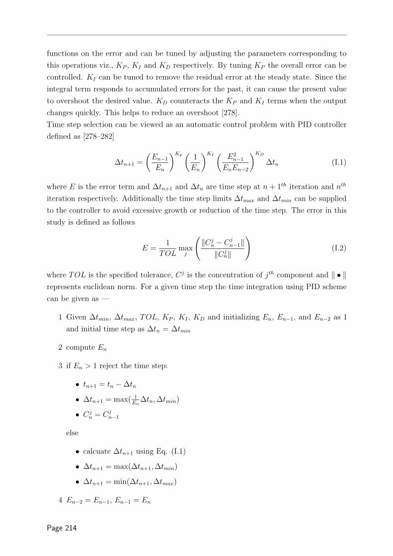
functions on the error and can be tuned by adjusting the parameters corresponding to

this operations viz., KP , KI and KD respectively. By tuning KP the overall error can be

controlled. KI can be tuned to remove the residual error at the steady state. Since the

integral term responds to accumulated errors for the past, it can cause the present value

to overshoot the desired value. KD counteracts the KP and KI terms when the output

changes quickly. This helps to reduce an overshoot [278].

Time step selection can be viewed as an automatic control problem with PID controller

defined as [278–282]

∆tn+1 =

(En−1

En

)Kp ( 1

En

)KI ( E2n−1

EnEn−2

)KD∆tn (I.1)

where E is the error term and ∆tn+1 and ∆tn are time step at n+ 1th iteration and nth

iteration respectively. Additionally the time step limits ∆tmax and ∆tmin can be supplied

to the controller to avoid excessive growth or reduction of the time step. The error in this

study is defined as follows

E =1

TOLmaxj

(‖Cj

n − Cjn−1‖

‖Cjn‖

)(I.2)

where TOL is the specified tolerance, Cj is the concentration of jth component and ‖ • ‖represents euclidean norm. For a given time step the time integration using PID scheme

can be given as —

1 Given ∆tmin, ∆tmax, TOL, KP , KI , KD and initializing En, En−1, and En−2 as 1

and initial time step as ∆tn = ∆tmin

2 compute En

3 if En > 1 reject the time step:

• tn+1 = tn −∆tn

• ∆tn+1 = max( 1En

∆tn,∆tmin)

• Cjn = Cj

n−1

else

• calcuate ∆tn+1 using Eq. (I.1)

• ∆tn+1 = max(∆tn+1,∆tmin)

• ∆tn+1 = min(∆tn+1,∆tmax)

4 En−2 = En−1, En−1 = En

Page 214

In case of LB schemes from Eq. (2.76) it can be deduced that ∆t ∝ (τ − 12). Hence the

PID controller can be heuristically rewritten in terms of relaxation parameter as(τn+1 −

1

2

)= SF

(En−1

En

)Kp ( 1

En

)KI ( E2n−1

EnEn−2

)KD (τn −

1

2

)(I.3)

In LB scheme resetting to previous time step in case of rejection requires an additional

storage of distribution functions which can be expensive in terms of memory. As a result

an additional safety factor SF is introduced in Eq. I.3 which can be tweaked to avoid

rejections. In case of rejection (if En+1 > 1), in present study the relaxation parameter is

taken as min(τn, τn+1).

Determination of PID control parameters is based on trial and error. In this study in

depth analysis of the PID parameters on accuracy of LB scheme was not carried out.

However based on preliminary investigation it was found that, the values PID parameters

(0.075, 0.175, and 0.08 for KP , KI and KD respectively) used by Valli et al. [281] for the

reactive flow and transport using finite element methods worked well for LB scheme too

and hence this values were used in this study. The value of relative tolerance was chosen

as 0.05 for C-S-H benchmark performed in chapter 8 and for the simulations of leaching

through micorstructures in chapter 8 the tolerance was further relaxed to 0.1. The value

of SF was taken as 0.9.

Page 215

References

Bibliography

[1] NIRAS, The cAt project in Dessel. A long-term solution for Belgian category A

waste, Tech. Rep. (NIRAS, 2010).

[2] NIRAS, Synthese van het veiligheidsrapport voor de opervlaktebergingsinrichting van

categorie-A afval in Dessel, Tech. Rep. (NIRAS, 2012).

[3] http://www.niras-cat.be/, accessed: 2015-09-24.

[4] P. K. Mehta and P. J. M. Monteiro, Concrete: microstructure, properties, and

materials (McGraw-Hill New York, 2006) p. 684.

[5] S. Bejaoui and B. Bary, Modeling of the link between microstructure and effective

diffusivity of cement pastes using a simplified composite model, Cement and Concrete

Research 37, 469 (2007).

[6] V. Ngala and C. Page, Effects of Carbonation on Pore Structure and Diffusional

Properties of Hydrated Cement Pastes, Cement and Concrete Research 27, 995

(1997).

[7] A. Delagrave, J. Marchand, and M. Pigeon, Influence of microstructure on the

tritiated water diffusivity of mortars, Advanced Cement Based Materials 7, 60 (1998).

[8] Q. T. Phung, Effects of carbonation and calcium leaching on microstructure and

transport properties of cement pastes, Ph.D. thesis, Ghent University (2015).

[9] H. Ma, D. Hou, J. Liu, and Z. Li, Estimate the relative electrical conductivity of

C-S-H gel from experimental results, Construction and Building Materials 71, 392

(2014).

Page 217

http://www.niras-cat.be/

http://dx.doi.org/10.1036/0071462899

http://dx.doi.org/10.1036/0071462899

http://dx.doi.org/10.1016/j.cemconres.2006.06.004


http://dx.doi.org/10.1016/S0008-8846(97)00102-6

http://dx.doi.org/10.1016/S0008-8846(97)00102-6

http://dx.doi.org/ 10.1016/S1065-7355(97)00029-1

http://dx.doi.org/ 10.1016/j.conbuildmat.2014.08.036


[10] M. Buil, E. Revertegat, and J. Oliver, A model of the attack of pure water or

undersaturated lime solution cement, in Stabilization and Solidification of Hazardous,

Radioactive, and Mixed Wastes, edited by T. M. Gilliam and C. C. Wiles (American

society for testing and materials, Philadelphia, 1992) 2nd ed., pp. 227–241.

[11] U. R. Berner, Modelling the incongruent dissolution of hydrated cement minerals,

Radiochimica Acta 44/45, 387 (1988).

[12] K. Wan, L. Li, and W. Sun, Solidliquid equilibrium curve of calcium in 6mol/L

ammonium nitrate solution, Cement and Concrete Research 53, 44 (2013).

[13] K. Haga, S. Sutou, M. Hironaga, S. Tanaka, and S. Nagasaki, Effects of porosity on

leaching of Ca from hardened ordinary Portland cement paste, Cement and Concrete

Research 35, 1764 (2005).

[14] S. Kamali, M. Moranville, and S. Leclercq, Material and environmental parameter

effects on the leaching of cement pastes: Experiments and modelling, Cement and

Concrete Research 38, 575 (2008).

[15] P. D. Tennis and H. M. Jennings, A model for two types of calcium silicate hydrate

in the microstructure of portland cement pastes, Cement and Concrete Research 30,

855 (2000).

[16] G. De Schutter, No concrete is sustainable without being durable, in International

Conference on Durability of Building Materials and Components - XIII DBMC,

edited by M. Quattrone and V. M. John (2015) p. 7.

[17] J. Tragaardh and B. Lagerblad, TR-98-11 Leaching of 90-year old concrete mortar

in contact with stagnant water, (1998).

[18] K. Yokozeki, K. Watanabe, N. Sakata, and N. Otsuki, Modeling of leaching from

cementitious materials used in underground environment, Applied Clay Science 26,

293 (2004).

[19] H. M. Jennings, J. J. Thomas, J. S. Gevrenov, G. Constantinides, and F. J. Ulm,

A multi-technique investigation of the nanoporosity of cement paste, Cement and


[20] J. J. Thomas and H. M. Jennings, A colloidal interpretation of chemical aging of the

C-S-H gel and its effects on the properties of cement paste, Cement and Concrete

Research 36, 30 (2006).

[21] H. M. Jennings, Refinements to colloid model of C-S-H in cement: CM-II, Cement

and Concrete Research 38, 275 (2008).

Page 218

http://dx.doi.org/ 10.1016/j.cemconres.2004.06.034




http://dx.doi.org/ 10.1016/j.clay.2003.12.027

http://dx.doi.org/ 10.1016/j.clay.2003.12.027







[22] H. M. Jennings, Colloid model of C-S-H and implications to the problem of creep

and shrinkage, Materials and Structures 37, 59 (2003).

[23] H. M. Jennings, A model for the microstructure of calcium silicate hydrate in cement

paste, Cement and Concrete Research 30, 101 (2000).

[24] H. M. Jennings, J. W. Bullard, J. J. Thomas, J. E. Andrade, J. J. Chen, and G. W.

Scherer, Characterization and Modeling of Pores and Surfaces in Cement Paste,

Journal of Advanced Concrete Technology 6, 5 (2008).

[25] H. M. Jennings and J. W. Bullard, From electrons to infrastructure: Engineering

concrete from the bottom up, Cement and Concrete Research 41, 727 (2011).

[26] D. Bentz, E. Garboczi, H. Jennings, and D. Quenard, Multi-scale digital-image-based

modelling of cement-based materials, in MRS Proceedings, Vol. 370 (Cambridge Univ

Press, 1994) p. 33.

[27] K. V. Breugel, Modelling of cement-based systems the alchemy of cement chemistry,

Cement and Concrete Research 34, 1661 (2004).

[28] J. S. Dolado and K. van Breugel, Recent advances in modeling for cementitious

materials, Cement and Concrete Research 41, 711 (2011).

[29] K. Maekawa, T. Ishida, and T. Kishi, Multi-scale Modeling of Concrete Perfor-

mance Integrated Material and Structural Mechanics, Journal Of Advanced Concrete

Technology 1, 91 (2003).

[30] E. A. B. Koenders, E. Schlangen, and K. V. Breugel, MULTI-SCALE MODELLING

: THE DELFTCODE, in International RILEM Symposium on Concrete Modelling

CONMOD08, May (2008) pp. 251–258.

[31] http://www.nist.gov/el/building_materials/electronic-monograph.cfm,

accessed: 2015-09-24.

[32] Z. Qian, Multiscale Modeling of Fracture Processes in Cementitious Materials, Ph.D.

thesis, TU Delft (2012).

[33] M. Zhang, Multiscale lattice Boltzman- finite element modelling of transport properties

in cement-based materials, Ph.D. thesis, TU Delft (2013).

[34] K. V. Breugel, Durability : Key issues in perspective, in 1st International Conference

on Microstructure Related Durability of Cementitious Composites 13-15 October

2008, October (2008) pp. 323–332.

Page 219

http://dx.doi.org/10.1617/14137

http://dx.doi.org/10.1016/S0008-8846(99)00209-4

http://dx.doi.org/10.3151/jact.6.5




http://www.nist.gov/el/building_materials/electronic-monograph.cfm

[35] S. Molins, D. Trebotich, C. I. Steefel, and C. Shen, An investigation of the effect

of pore scale flow on average geochemical reaction rates using direct numerical

simulation, Water Resources Research 48, 1 (2012).

[36] L. Li, C. a. Peters, and M. a. Celia, Upscaling geochemical reaction rates using

pore-scale network modeling, Advances in Water Resources 29, 1351 (2006).

[37] A. Raoof, H. Nick, T. Wolterbeek, and C. Spiers, Pore-scale modeling of reactive

transport in wellbore cement under CO2 storage conditions, International Journal of

Greenhouse Gas Control 11, S67 (2012).

[38] E. M. Ryan, A. M. Tartakovsky, and C. Amon, Pore-scale modeling of competitive

adsorption in porous media. Journal of contaminant hydrology 120-121, 56 (2011).

[39] A. M. Tartakovsky, P. Meakin, T. D. Scheibe, and B. D. Wood, A smoothed particle

hydrodynamics model for reactive transport and mineral precipitation in porous and

fractured porous media, Water Resources Research 43, W05437 (2007).

[40] G. O’Brien and C. Bean, A comparison of published experimental data with a coupled

lattice Boltzmann-analytic advection-diffusion method for reactive transport in porous

media, Journal of Hydrology 268, 143 (2002).

[41] R. Verberg and A. J. C. Ladd, Simulation of chemical erosion in rough fractures,

Physical Review E 65, 1 (2002).

[42] H. Yoon, A. J. Valocchi, C. J. Werth, and T. Dewers, Pore-scale simulation of

mixing-induced calcium carbonate precipitation and dissolution in a microfluidic pore

network, Water Resources Research 48, 1 (2012).

[43] D. Yu and A. J. C. Ladd, A numerical simulation method for dissolution in porous

and fractured media, Journal of Computational Physics 229, 6450 (2010).

[44] Q. Kang, P. C. Lichtner, and D. Zhang, Lattice Boltzmann pore-scale model for

multicomponent reactive transport in porous media, Journal of Geophysical Research:

Solid Earth 111, 1 (2006).

[45] Q. Kang, P. C. Lichtner, and D. Zhang, An improved lattice Boltzmann model for

multicomponent reactive transport in porous media at the pore scale, Water Resources

Research 43, 1 (2007).

[46] Q. Kang, P. C. Lichtner, and D. R. Janecky, Lattice boltzmann method for reacting

flows in porous media, Advances in Applied Mathematics and Mechanics 2, 545

(2010).

Page 220

http://dx.doi.org/10.1029/2011WR011404

http://dx.doi.org/ 10.1016/j.advwatres.2005.10.011

http://dx.doi.org/10.1016/j.ijggc.2012.09.012

http://dx.doi.org/10.1016/j.ijggc.2012.09.012

http://dx.doi.org/ 10.1016/j.jconhyd.2010.06.008

http://dx.doi.org/10.1029/2005WR004770

http://www.sciencedirect.com/science/article/pii/S0022169402001737

http://dx.doi.org/ 10.1103/PhysRevE.65.056311

http://dx.doi.org/10.1029/2011WR011192

http://dx.doi.org/10.1016/j.jcp.2010.05.005

http://dx.doi.org/10.1029/2005JB003951

http://dx.doi.org/10.1029/2005JB003951

http://dx.doi.org/10.1029/2006WR005551

http://dx.doi.org/10.1029/2006WR005551

http://dx.doi.org/10.4208/aamm.10-10S02

http://dx.doi.org/10.4208/aamm.10-10S02

[47] S. Sullivan, F. Sani, M. Johns, and L. Gladden, Simulation of packed bed reactors

using lattice Boltzmann methods, Chemical Engineering Science 60, 3405 (2005).

[48] X. Zhang, J. W. Crawford, and I. M. Young, Does pore water velocity affect the

reaction rates of adsorptive solute transport in soils? Demonstration with pore-scale

modelling, Advances in Water Resources 31, 425 (2008).

[49] F. Verhaeghe, S. Arnout, B. Blanpain, and P. Wollants, Lattice-Boltzmann modeling

of dissolution phenomena, Physical Review E - Statistical, Nonlinear, and Soft Matter

Physics 73, 036316 (2006).

[50] F. Verhaeghe, J. Liu, M. Guo, S. Arnout, B. Blanpain, and P. Wollants, Dissolution

and diffusion behavior of Al2O3 in a CaO- Al2O3-SiO2 liquid: An experimental-

numerical approach, Applied Physics Letters 91, 124104 (2007).

[51] A. Hiorth, E. Jettestuen, L. Cathles, and M. Madland, Precipitation, dissolution,

and ion exchange processes coupled with a lattice Boltzmann advection diffusion

solver, Geochimica et Cosmochimica Acta 104, 99 (2013).

[52] K. Van Breugel, Simulation of hydration and formation of structure in hardening

cement-based materials, Ph.D. thesis, TU Delft (1991).

[53] J. Thomas, J. Biernacki, and J. Bullard, Modeling and simulation of cement hydration

kinetics and microstructure development, Cement and Concrete Research 41, 1257

(2011).

[54] G. Ye, Experimental Study and Numerical Simulation of the Development of the

Microstructure and Permeability of Cementitious Materials, Ph.D. thesis, TU Delft

(2003).

[55] S. Bishnoi and K. Scrivener, Micro-Structural Modelling of cementitious materials

using vector approach, in Congress on the Chemistry of Cement (2007).

[56] S. Bishnoi and K. L. Scrivener, µic : A new platform for modelling the hydration of

cements, Cement and Concrete Research 39, 266 (2009).

[57] C. Pignat, P. Navi, and K. Scrivener, Simulation of cement paste microstructure

hydration, pore space characterization and permeability determination, Materials and

Structures 38, 459 (2005).

[58] P. Navi and C. Pignat, Three-dimensional characterization of the pore structure of a

simulated cement paste, Cement and Concrete Research 29, 507 (1999).

Page 221

http://dx.doi.org/10.1016/j.ces.2005.01.038


http://dx.doi.org/10.1103/PhysRevE.73.036316


http://dx.doi.org/ 10.1063/1.2786854

http://dx.doi.org/10.1016/j.gca.2012.11.019




http://dx.doi.org/10.1617/14355

http://dx.doi.org/10.1617/14355

http://dx.doi.org/10.1016/S0008-8846(98)00199-9

[59] D. Bentz, P. Coveney, E. Garboczi, M. Kleyn, and P. Stutzman, Cellular automaton

simulations of cement hydration and microstructure development, Modelling and

Simulation in Materials Science and Engineering 2, 783 (1994).

[60] J. W. Bullard, E. Enjolras, W. L. George, S. G. Satterfield, and J. E. Terrill, A

parallel reaction-transport model applied to cement hydration and microstructure

development, Modelling and Simulation in Materials Science and Engineering 18,

025007 (2010).

[61] http://www.citg.tudelft.nl/index.php?id=17650&L=1, accessed: 2015-09-24.

[62] http://www.nist.gov/el/building_materials/evcctl.cfm, accessed: 2015-09-

24.

[63] N. Van Tuan, Rice husk ash as a mineral admixture for ultra high performance

concrete, Ph.D. thesis, Tu Delft (2011).

[64] D. L. Parkhurst and C. Appelo, Description of Input and Examples for PHREEQC

Version 3 A Computer Program for Speciation , Batch-Reaction , One-Dimensional

Transport , and Inverse Geochemical Calculations Chapter 43 of, in Modeling Tech-

niques (2013) Chap. chap. A43, pp. 1–678.

[65] U. Frisch, B. Hasslacher, and Y. Pomeau, Lattice-Gas Automata for the Navier-

Stokes Equation, Physical Review Letters 56, 1505 (1986).

[66] F. J. Higuera and J. Jimenez, Boltzmann Approach to Lattice Gas Simulations,

Europhysics Letters (EPL) 9, 663 (1989).

[67] F. Higuera, S. Succi, and R. Benzi, Lattice gas dynamics with enhanced collisions,

Europhysics Letters (EPL) 9, 345 (1989).

[68] Y. Qian, D. D’Humieres, and P. Lallemand, Lattice BGK models for Navier-Stokes

equation, Europhysics Letters (EPL) 17, 479 (1992).

[69] P. Bhatnagar, E. Gross, and M. Krook, A model for collision processes in gases. I.

Small amplitude processes in charged and neutral one-component systems, Physical

review 94, 511 (1954).

[70] D. D’Humieres, I. Ginzburg, M. Krafczyk, P. Lallemand, and L.-S. Luo, Philosoph-

ical Transactions of the Royal Society of London A: Mathematical, Physical and

Engineering Sciences 360, 437 (2002).

[71] E. Flekkoy, Lattice Bhatnagar-Gross-Krook models for miscible fluids, Physical

Review E 47, 4247 (1993).

Page 222

http://iopscience.iop.org/0965-0393/2/4/001

http://iopscience.iop.org/0965-0393/2/4/001

http://dx.doi.org/10.1088/0965-0393/18/2/025007

http://dx.doi.org/10.1088/0965-0393/18/2/025007

http://www.citg.tudelft.nl/index.php?id=17650&L=1

http://www.nist.gov/el/building_materials/evcctl.cfm

http://pubs.usgs.gov/tm/06/a43/

http://pubs.usgs.gov/tm/06/a43/

http://dx.doi.org/10.1103/PhysRevLett.56.1505

http://prola.aps.org/abstract/PR/v94/i3/p511_1

http://prola.aps.org/abstract/PR/v94/i3/p511_1

http://dx.doi.org/10.1098/rsta.2001.0955



[72] H. Chen, I. Goldhirsch, and S. A. Orszag, Discrete Rotational Symmetry, Mo-

ment Isotropy, and Higher Order Lattice Boltzmann Models, Journal of Scientific

Computing 34, 87 (2007).

[73] I. Ginzburg, Equilibrium-type and link-type lattice Boltzmann models for generic

advection and anisotropic-dispersion equation, Advances in Water Resources 28, 1171

(2005).

[74] B. Servan-Camas, Lattice Boltzmann modeling for mass transport equations in porous

media, Ph.D. thesis, Louisiana State University and Agricultural and Mechanical

College (2008).

[75] J. Latt, Hydrodynamic limit of lattice Boltzmann equations, Ph.D. thesis, Universite

De Geneve (2007).

[76] J. Latt, Technical report : How to implement your DdQq dynamics with only q

variables per node (instead of 2q), Tech. Rep. 1 (2007).

[77] K. Mattila, J. Hyvaluoma, J. Timonen, and T. Rossi, Comparison of implementations

of the lattice-Boltzmann method, Computers & Mathematics with Applications 55,

1514 (2008).

[78] M. Wittmann, T. Zeiser, G. Hager, and G. Wellein, Comparison of different

propagation steps for lattice Boltzmann methods, Computers & Mathematics with

Applications 65, 924 (2013).

[79] S. Suga, Numerical schemes obtained From lattice Boltzmann equations for advection

Diffusion Equations, International Journal of Modern Physics C 17, 1563 (2006).

[80] P. Lallemand and L.-S. Luo, Theory of the lattice Boltzmann method: dispersion,

dissipation, isotropy, Galilean invariance, and stability, Physical review. E 61, 6546

(2000).

[81] H. Yoshida and M. Nagaoka, Multiple-relaxation-time lattice Boltzmann model for

the convection and anisotropic diffusion equation, Journal of Computational Physics

229, 7774 (2010).

[82] R. Cornubert, D. D’Humieres, and D. Levermore, A Knudsen layer theory for lattice

gases, Physica D: Nonlinear Phenomena 47, 241 (1991).

[83] D. Ziegler, Boundary conditions for lattice Boltzmann simulations, Journal of Statis-

tical Physics 71, 1171 (1993).

Page 223

http://etd.lsu.edu/docs/available/etd-11072008-084923/

http://www.palabos.org/palabos/downloads/plb-tr1.pdf

http://www.palabos.org/palabos/downloads/plb-tr1.pdf

http://dx.doi.org/10.1016/j.camwa.2007.08.001






http://dx.doi.org/ 10.1016/j.jcp.2010.06.037

http://dx.doi.org/ 10.1016/j.jcp.2010.06.037

http://dx.doi.org/ 10.1016/0167-2789(91)90295-K

http://link.springer.com/article/10.1007/BF01049965

http://link.springer.com/article/10.1007/BF01049965

[84] M. A. Gallivan, D. R. Noble, J. G. Georgiadis, and R. O. Buckius, an Evalua-

tion of the BounceBack Boundary Condition for Lattice Boltzmann Simulations,

International Journal for Numerical Methods in Fluids 25, 249 (1997).

[85] D. Kandhai, A. Koponen, A. Hoekstra, M. Kataja, J. Timonen, and P. Sloot,

Implementation aspects of 3D lattice-BGK: boundaries, accuracy, and a new Fast

relaxation method, Journal of Computational Physics 150, 482 (1999).

[86] C. Pan, L.-S. Luo, and C. T. Miller, An evaluation of lattice Boltzmann schemes

for porous medium flow simulation, Computers & Fluids 35, 898 (2006).

[87] L. Talon, D. Bauer, N. Gland, S. Youssef, H. Auradou, and I. Ginzburg, Assessment

of the two relaxation time Lattice-Boltzmann scheme to simulate Stokes flow in

porous media, Water Resources Research 48 (2012), 10.1029/2011WR011385.

[88] S. Khirevich, I. Ginzburg, and U. Tallarek, Coarse- and fine-grid numerical behavior

of MRT/TRT lattice-Boltzmann schemes in regular and random sphere packings,

Journal of Computational Physics 281, 708 (2015).

[89] I. Ginzburg, D. D’Humieres, and A. Kuzmin, Optimal stability of advection-diffusion

lattice boltzmann models with two relaxation times for positive/negative equilibrium,

Journal of Statistical Physics 139, 1090 (2010).

[90] B. Servan-Camas and F. T. C. Tsai, Lattice Boltzmann method with two relaxation

times for advection-diffusion equation: Third order analysis and stability analysis,

Advances in Water Resources 31, 1113 (2008).

[91] A. Kuzmin, I. Ginzburg, and A. Mohamad, The role of the kinetic parameter in

the stability of two-relaxation-time advectiondiffusion lattice Boltzmann schemes,

Computers & Mathematics with Applications 61, 3417 (2011).

[92] I. Ginzburg, Consistent lattice Boltzmann schemes for the Brinkman model of

porous flow and infinite Chapman-Enskog expansion, Physical Review E - Statistical,

Nonlinear, and Soft Matter Physics 77, 1 (2008).

[93] J. Perko and R. A. Patel, Single relaxation time lattice Boltzmann scheme for

advective-diffusion problems with large diffusion coeffcient heterogeneities and high

advective transport, Physical Review E 89, 053309 (2014).

[94] Lattice dependence of reaction-diffusion in lattice Boltzmann modeling, Computer

Physics Communications 129, 256 (2000).

[95] P. K. Smolarkiewicz, A simple positive definite advection scheme with small implicit

diffusion, Monthly Weather Review 11, 479 (1983).

Page 224

http://dx.doi.org/ 10.1002/(SICI)1097-0363(19970815)25:3<249::AID-FLD546>3.3.CO;2-Z

http://dx.doi.org/ 10.1006/jcph.1999.6191

http://dx.doi.org/ 10.1029/2011WR011385

http://dx.doi.org/10.1016/j.jcp.2014.10.038

http://dx.doi.org/ 10.1007/s10955-010-9969-9





[96] E. Wexler, Analytical solutions for one-, two-, and three-dimensional solute transport

in ground-water systems with uniform flow , Tech. Rep. ([Washington, D.C.] :, 1992).

[97] D. D’Humieres and P. Lallemand, Numerical simulations of hydrodynamics with

lattice gas automata in two dimensions, Complex Systems 1, 599 (1987).

[98] P. Lavallee, J. P. Boon, and N. Alain, Lattice Boltzmann Equation for Laminar

Boundary flow, Complex Systems 3, 317 (1989).

[99] T. Zhang, B. Shi, Z. Guo, Z. Chai, and J. Lu, General bounce-back scheme for

concentration boundary condition in the lattice-Boltzmann method, Physical Review

E 85, 016701:1 (2012).

[100] I. Ginzburg, Generic boundary conditions for lattice Boltzmann models and their

application to advection and anisotropic dispersion equations, Advances in Water

Resources 28, 1196 (2005).

[101] Z. Guo, C. Zheng, and B. Shi, An extrapolation method for boundary conditions in

lattice Boltzmann method, Physics of Fluids 14, 2007 (2002).

[102] Z. Guo, B. Shi, and C. Zheng, A coupled lattice BGK model for the Boussinesq

equations, International Journal for Numerical Methods in Fluids 39, 325 (2002).

[103] J. Latt, B. Chopard, O. Malaspinas, M. Deville, and A. Michler, Straight velocity

boundaries in the lattice Boltzmann method, Physical Review E - Statistical, Nonlinear,

and Soft Matter Physics 77 (2008), 10.1103/PhysRevE.77.056703.

[104] H.-B. Huang, X.-Y. Lu, and M. C. Sukop, Numerical study of lattice Boltzmann

methods for a convectiondiffusion equation coupled with NavierStokes equations,

Journal of Physics A: Mathematical and Theoretical 44, 055001 (2011).

[105] J. Vazquez, The Porous Medium Equation: Mathematical Theory , Oxford Mathe-

matical Monographs (Clarendon Press, 2007).

[106] S. Ghosh, K. Lee, and P. Raghavan, A multi-level computational model for multi-

scale damage analysis in composite and porous materials, International Journal of

Solids and Structures 38, 2335 (2001).

[107] A. Vikhansky and I. Ginzburg, Taylor dispersion in heterogeneous porous media:

Extended method of moments, theory, and modelling with two-relaxation-times lattice

Boltzmann scheme, Physics of Fluids 26, 022104 (2014).

[108] X. Zhang, a. G. Bengough, L. K. Deeks, J. W. Crawford, and I. M. Young, A novel

three-dimensional lattice Boltzmann model for solute transport in variably saturated

porous media, Water Resources Research 38, 6 (2002).

Page 225

http://pubs.usgs.gov/twri/twri3-b7/

http://pubs.usgs.gov/twri/twri3-b7/

https://www.complex-systems.com/pdf/01-4-5.pdf http://www.complex-systems.com/

http://www.complex-systems.com/abstracts/v03_i04_a01.html





http://dx.doi.org/ 10.1063/1.1471914

http://dx.doi.org/10.1002/fld.337



http://dx.doi.org/ 10.1088/1751-8113/44/5/055001

http://books.google.be/books?id=4E2Gc67b-dYC

http://dx.doi.org/http://dx.doi.org/10.1016/S0020-7683(00)00167-0

http://dx.doi.org/http://dx.doi.org/10.1016/S0020-7683(00)00167-0

http://dx.doi.org/10.1063/1.4864631

http://dx.doi.org/10.1029/2001WR000982

[109] S. D. C. Walsh and M. O. Saar, Macroscale lattice-Boltzmann methods for low Peclet

number solute and heat transport in heterogeneous porous media, Water Resources

Research 46, W07517 (2010).

[110] P. Lichtner, Continuum formulation of multicomponent-multiphase reactive transport,

Reviews in Mineralogy and Geochemistry 34, 1996 (1996).

[111] C. Appelo and D. Postma, Geochemistry, Groundwater and Pollution, 2nd ed. (CRC

Press, 2005).

[112] C. I. Steefel, C. A. J. Appelo, B. Arora, D. Jacques, T. Kalbacher, O. Kolditz,

V. Lagneau, P. C. Lichtner, K. U. Mayer, J. C. L. Meeussen, S. Molins, D. Moulton,

H. Shao, J. Simnek, N. Spycher, S. B. Yabusaki, and G. T. Yeh, Reactive transport

codes for subsurface environmental simulation, Computational Geosciences 19, 445

(2014).

[113] M. Dentz, T. Le Borgne, A. Englert, and B. Bijeljic, Mixing, spreading and reaction

in heterogeneous media: a brief review. Journal of contaminant hydrology 120-121,

1 (2011).

[114] C. I. Steefel and K. Maher, Fluid-Rock Interaction: A Reactive Transport Approach,

Reviews in Mineralogy and Geochemistry 70, 485 (2009).

[115] C. I. Steefel and K. T. B. MacQuarrie, Approaches to modeling of reactive transport

in porous media, Reviews in Mineralogy and Geochemistry 34, 85 (1996).

[116] P. J. Dellar, An interpretation and derivation of the lattice Boltzmann method using

Strang splitting, Computers and Mathematics with Applications 65, 129 (2013).

[117] R. A. Patel, J. Perko, D. Jacques, G. De Schutter, K. Van Breugel, and G. Ye,

A versatile pore-scale multicomponent reactive transport approach based on lattice

Boltzmann method: Application to portlandite dissolution, Physics and Chemistry of

the Earth 70-71, 127 (2014).

[118] R. A. Patel, J. Perko, D. Jacques, G. De Schutter, G. Ye, and K. V. Breugel, Lattice

Boltzmann based multicomponent reactive transport model coupled with geochemical

solver for pore scale simulations, in V International Conference on Computational

Methods for Coupled Problems in Science and Engineering, COUPLED PROBLEMS

2013, edited by S. Idelsohn, M. Papadrakakis, and B. Schrefler (CIMNE, Barcelona,

Ibiza, Spain, 2013) pp. 806–817.

[119] J. Allison, D. Brown, and K. Novo-Gradac, MINTEQA2/PRODEFA2, A Geograph-

ical Assessment Model For Environmental Systems: Version 3.0 User’s Manual ,

Tech. Rep. (Environmental Research Laboratory, Georgia, USA, 1991).

Page 226

http://dx.doi.org/ 10.1029/2009WR007895

http://dx.doi.org/ 10.1029/2009WR007895

http://rimg.geoscienceworld.org/content/34/1/1.citation

https://books.google.be/books/about/Geochemistry_Groundwater_and_Pollution_S.html?id=k1jSyuEpzEwC&pgis=1

http://dx.doi.org/10.1007/s10596-014-9443-x

http://dx.doi.org/10.1007/s10596-014-9443-x



http://dx.doi.org/ 10.2138/rmg.2009.70.11

http://rimg.geoscienceworld.org/content/34/1/85.short


http://dx.doi.org/10.1016/j.pce.2014.03.001

http://dx.doi.org/10.1016/j.pce.2014.03.001

http://www2.epa.gov/exposure-assessment-models/minteqa2prodefa2-geographical-assessment-model-environmental-systems

http://www2.epa.gov/exposure-assessment-models/minteqa2prodefa2-geographical-assessment-model-environmental-systems

[120] Bethke, C.M., and Yeakel, The Geochemist’s Workbench User’s Guides, Version

9.0., Tech. Rep. (Aqueous Solutions LLC, Champaign, IL, 2011).

[121] D. A. Kulik, T. Wagner, S. V. Dmytrieva, G. Kosakowski, F. F. Hingerl, K. V.

Chudnenko, and U. R. Berner, GEM-Selektor geochemical modeling package: Revised

algorithm and GEMS3K numerical kernel for coupled simulation codes, Computa-

tional Geosciences 17, 1 (2013).

[122] H. S. Carslow and J. C. Jaeger, Conduction of Heat in Solids (Oxford Uni. Press,

Newyork, 1986) p. 378.

[123] D. Jacques, L. Wang, E. Martens, and D. Mallants, Modelling chemical degradation

of concrete during leaching with rain and soil water types, Cement and Concrete

Research 40, 1306 (2010).

[124] B. Lothenbach, Thermodynamic equilibrium calculations in cementitious systems,

Materials and Structures 43, 1413 (2010).

[125] D. Jacques, Benchmarking of the cement model and detrimental chemical reactions

including temperature dependent parameters, Tech. Rep. (NIROND-TR report 200830

E, SCK•CEN, 2009).

[126] B. Lothenbach, T. Matschei, G. Moschner, and F. Glasser, Thermodynamic modelling

of the effect of temperature on the hydration and porosity of Portland cement, Cement


[127] S. R. Charlton and D. L. Parkhurst, Modules based on the geochemical model

PHREEQC for use in scripting and programming languages, Computers & Geo-

sciences 37, 1653 (2011).

[128] H. Aaron, D. Fainstein, and G. Kotler, DiffusionLimited Phase Transformations: A

Comparison and Critical Evaluation of the Mathematical Approximations, Journal of

applied physics 41, 4404 (1970).

[129] L. Wissmeier and D. Barry, Simulation tool for variably saturated flow with compre-

hensive geochemical reactions in two- and three-dimensional domains, Environmental

Modelling & Software 26, 210 (2011).

[130] R. J. Millington and J. P. Quirk, Permeability of porous solids, Transactions of the

Faraday Society 57, 1200 (1961).

[131] D. A. Kulik, Improving the structural consistency of C-S-H solid solution thermody-

namic models, Cement and Concrete Research 41, 477 (2011).

Page 227

http://www.gwb.com/documentation.php

http://www.gwb.com/documentation.php

http://dx.doi.org/10.1007/s10596-012-9310-6

http://dx.doi.org/10.1007/s10596-012-9310-6

http://dx.doi.org/10.1115/1.3225900

http://dx.doi.org/10.1617/s11527-010-9592-x



http://dx.doi.org/10.1016/j.cageo.2011.02.005

http://dx.doi.org/10.1016/j.cageo.2011.02.005

http://dx.doi.org/10.1063/1.1658474

http://dx.doi.org/10.1063/1.1658474

http://dx.doi.org/ 10.1016/j.envsoft.2010.07.005

http://dx.doi.org/ 10.1016/j.envsoft.2010.07.005

http://dx.doi.org/ 10.1039/tf9615701200

http://dx.doi.org/ 10.1039/tf9615701200


[132] D. Jacques, J. Simnek, D. Mallants, and M. T. van Genuchten, Operator-splitting

errors in coupled reactive transport codes for transient variably saturated flow and

contaminant transport in layered soil profiles. Journal of contaminant hydrology 88,

197 (2006).

[133] R. A. Patel, J. Perko, D. Jacques, G. De Schutter, G. Ye, and K. V. BREUGEL,

application of porescale reactive transport model to study the influence of pore network

characteristics on calcium leaching in cementitious material, in CONMOD 2014

(Beijing, China, 2014) pp. 359–366.

[134] M. Wang, J. Wang, N. Pan, and S. Chen, Mesoscopic predictions of the effective

thermal conductivity for microscale random porous media, Physical Review E 75,

036702 (2007).

[135] G. Van Der Wegen, R. B. Polder, and K. Van Breugel, Guideline for service life

design of structural concrete - A performance based approach with regard to chloride

induced corrosion, Heron 57, 153 (2012).

[136] C. D. Shackelford and D. E. Daniel, Diffusion in Saturated Soil. I: Background,

Journal of Geotechnical Engineering 117, 467 (1991).

[137] E. J. Garboczi and D. P. Bentz, Computer simulation of the diffusivity of cement-

based materials, Journal of Materials Science 27, 2083 (1992).

[138] Y. Ichikawa, K. Kawamura, N. Fujii, and T. Nattavut, Molecular dynamics and

multiscale homogenization analysis of seepage/diffusion problem in bentonite clay,

International Journal for Numerical Methods in Engineering 54, 1717 (2002).

[139] S. Numata, H. Amano, and K. Minami, Diffusion of tritiated water in cement

materials, Journal of Nuclear Materials 171, 373 (1990).

[140] E. Revertegat, C. Richet, and P. Gegout, Effect of pH on the durability of cement

pastes, Cement and Concrete Research 22, 259 (1992).

[141] M. Castellote, C. Alonso, C. Andrade, G. a. Chadbourn, and C. L. Page, Oxygen and

chloride diffusion in cement pastes as a validation of chloride diffusion coefficients

obtained by steady-state migration tests, Cement and Concrete Research 31, 621

(2001).

[142] T. Yamaguchi, K. Negishi, S. Hoshino, and T. Tanaka, Modeling of diffusive mass

transport in micropores in cement based materials, Cement and Concrete Research

39, 1149 (2009).

Page 228





http://dx.doi.org/ 10.1061/(ASCE)0733-9410(1991)117:3(467)

http://dx.doi.org/ 10.1007/BF01117921

http://dx.doi.org/ 10.1002/nme.488

http://dx.doi.org/10.1016/0022-3115(90)90383-X

http://dx.doi.org/ 10.1016/0008-8846(92)90064-3

http://dx.doi.org/10.1016/S0008-8846(01)00469-0

http://dx.doi.org/10.1016/S0008-8846(01)00469-0



[143] P. Tumidajski, A. S. Schumacher, S. Perron, P. Gu, and J. Beaudoin, On the

relationship between porosity and electrical resistivity in cementitous systems, Cement


[144] G. G. Taffinder and B. Batchelor, Measurement of effective diffusivities in solidified

wastes, Journal of Environmental Engineering 119, 17 (1993).

[145] B. J. Christensen, T. O. Mason, H. M. Jennings, D. P. Bentz, and E. J. Garboczi,

Experimental and computer simulation results for the electrical conductivity of

portland cement paste, Materials Research Society Symposium Proceeding 245, 259

(1992).

[146] B. H. Oh and S. Y. Jang, Prediction of diffusivity of concrete based on simple analytic

equations, Cement and Concrete Research 34, 463 (2004).

[147] G.-W. Sun, W. Sun, Y.-s. Zhang, and Z.-y. Liu, Relationship between chloride

diffusivity and pore structure of hardened cement paste, Journal of Zhejiang University

SCIENCE A 12, 360 (2011).

[148] T. C. Hansen, Physical structure of hardened cement paste, Materials and Structures

19, 423 (1986).

[149] D. P. Bentz and E. J. Garboczi, Percolation of phases in a tiiree-dimensional cement

paste microstructural model, Cement and Concrete Research 21, 325 (1991).

[150] R. Spragg, C. Villani, K. Snyder, D. Bentz, J. W. Bullard, and J. Weiss, Factors that

influence electrical resistivity measurements in cementitious Systems, Transportation

Research Record: Journal of the Transportation Research Board 2342, 90 (2013).

[151] G. Archie, The electrical resistivity log as an aid in determining some reservoir

characteristics, Trans.Transactions of the American institute of mineralogy and

metallurgy 146, 54 (1942), arXiv:942054-G [10.2118] .

[152] K. K. Aligizaki, Pore structure of cement-based materials: testing, interpretation

and requirements (CRC Press, 2005) p. 432.

[153] A. Atkinson and A. K. Nickerson, The diffusion of ions through water-saturated

cement, Journal of Materials Science 19, 3068 (1984).

[154] J. M. Galındez and J. Molinero, Assessment of the long-term stability of cementitious

barriers of radioactive waste repositories by using digital-image-based microstructure

generation and reactive transport modelling, Cement and Concrete Research 40, 1278

(2010).

Page 229



http://dx.doi.org/ 10.1631/jzus.A1000413

http://dx.doi.org/ 10.1631/jzus.A1000413

http://dx.doi.org/10.3141/2342-11

http://dx.doi.org/10.3141/2342-11

http://dx.doi.org/10.2118/942054-G

http://dx.doi.org/10.2118/942054-G

http://arxiv.org/abs/942054-G

https://books.google.com/books?hl=en&lr=&id=P-DGDRfAk8MC&pgis=1

https://books.google.com/books?hl=en&lr=&id=P-DGDRfAk8MC&pgis=1

http://dx.doi.org/ 10.1007/BF01026986



[155] W. O. Winsauer, H. M. Shearin Jr., P. H. Masson, and M. Williams, Resistivity of

Brine-Saturated Sands in Relation to Pore Geometry, (1952).

[156] J. V. D. Lee, L. D. Windt, and V. Lagneau, Application of reactive transport models

in cement based porous media, in International RILEM Symposium on Concrete

Modelling CONMOD08, May (2008) pp. 463–470.

[157] M. Mainguy, C. Tognazzi, J. M. Torrenti, and F. Adenot, Modelling of leaching in

pure cement paste and mortar, Cement and Concrete Research 30, 83 (2000).

[158] J. Walton, L. Plansky, and R. Smith, Models for estimation of service life of

concrete barriers in low-level radioactive waste disposal , Tech. Rep. (Idaho National

Engineering Laboratory (United States), 1990).

[159] D. P. Bentz, E. J. Garboczi, C. J. Haecker, and O. M. Jensen, Effects of cement par-

ticle size distribution on performance properties of Portland cement-based materials,


[160] G. Ye, Percolation of capillary pores in hardening cement pastes, Cement and


[161] G. Ye and K. Van Breugel, Three-dimensional microstructure simulation model of

cement based materials, Heron 48, 251 (2003).

[162] E. J. Garboczi and D. P. Bentz, The effect of statistical fluctuation, finite size error,

and digital resolution on the phase percolation and transport properties of the NIST

cement hydration model, Cement and Concrete Research 31, 1501 (2001).

[163] S. Torquato, Random Heterogeneous Materials: Microstructure and Macroscopic

Properties (Springer Science & Business Media, 2013) p. 703.

[164] P. Pivonka, C. Hellmich, and D. Smith, Microscopic effects on chloride diffusivity

of cement pastes-a scale-transition analysis, Cement and Concrete Research 34, 2251

(2004).

[165] B. Bary and S. Bejaoui, Assessment of diffusive and mechanical properties of hardened

cement pastes using a multi-coated sphere assemblage model, Cement and Concrete

Research 36, 245 (2006).

[166] G. W. Milton, Concerning bounds on the transport and mechanical properties of

multicomponent composite materials, Applied Physics A Solids and Surfaces 26, 125

(1981).

[167] E. Stora, B. Bary, and Q. C. He, On estimating the effective diffusive properties of

hardened cement pastes, Transport in Porous Media 73, 279 (2008).

Page 230

http://dx.doi.org/10.1306/3D9343F4-16B1-11D7-8645000102C1865D

http://dx.doi.org/10.1306/3D9343F4-16B1-11D7-8645000102C1865D

http://dx.doi.org/10.1016/S0008-8846(99)00208-2

http://dx.doi.org/10.2172/6548946

http://dx.doi.org/10.2172/6548946

http://dx.doi.org/10.1016/S0008-8846(99)00163-5



http://dx.doi.org/10.1016/S0008-8846(01)00593-2

https://books.google.com/books?id=UTfoBwAAQBAJ&pgis=1

https://books.google.com/books?id=UTfoBwAAQBAJ&pgis=1





http://dx.doi.org/10.1007/BF00616659

http://dx.doi.org/10.1007/BF00616659

http://dx.doi.org/ 10.1007/s11242-007-9170-z

[168] E. Stora, Q.-C. He, and B. Bary, A mixed composite spheres assemblage model

for the transport properties of random heterogeneous materials with high contrasts,

Journal of Applied Physics 100, 084910 (2006).

[169] E. Stora, B. Bary, Q.-C. He, E. Deville, and P. Montarnal, Modelling and simulations

of the chemo-mechanical behaviour of leached cement-based materials, Cement and


[170] W. Dridi, Analysis of effective diffusivity of cement based materials by multi-scale

modelling, Materials and Structures , 313 (2012).

[171] X. Liu, R. Lackner, and C. Pichler, Highlighting the effect of gel-Pore diffusivity on

the effective diffusivity of cement paste A multiscale investigation, in Computational

Structural Engineering, edited by Y. Uan, J. Cui, and H. A. Mang (Springer

Netherlands, 2009) pp. 973–981.

[172] O. Bernard, F. J. Ulm, and E. Lemarchand, A multiscale micromechanics-hydration

model for the early-age elastic properties of cement-based materials, Cement and


[173] S. Kamali-Bernard, F. Bernard, and W. Prince, Computer modelling of tritiated

water diffusion test for cement based materials, Computational Materials Science

45, 528 (2009).

[174] N. Ukrainczyk and E. A. B. Koenders, Representative elementary volumes for 3D

modeling of mass transport in cementitious materials, Modelling and Simulation in

Materials Science and Engineering 22, 035001 (2014).

[175] M. Zhang, G. Ye, and K. Van Breugel, Microstructure-based modeling of water

diffusivity in cement paste, Construction and Building Materials 25, 2046 (2011).

[176] L. Liu, H. Chen, W. Sun, and G. Ye, Microstructure-based modeling of the diffusivity

of cement paste with micro-cracks, Construction and Building Materials 38, 1107

(2013).

[177] L. Liu, W. Sun, G. Ye, H. Chen, and Z. Qian, Estimation of the ionic diffusivity of

virtual cement paste by random walk algorithm, Construction and Building Materials

28, 405 (2012).

[178] M. Zhang, G. Ye, and K. Van Breugel, Modeling of ionic diffusivity in non-saturated

cement-based materials using lattice Boltzmann method, Cement and Concrete Re-

search 42, 1524 (2012).

Page 231

http://dx.doi.org/10.1063/1.2360155



http://dx.doi.org/10.1617/s11527-012-9903-5

http://dx.doi.org/10.1016/S0008-8846(03)00039-5

http://dx.doi.org/10.1016/S0008-8846(03)00039-5

http://dx.doi.org/10.1016/j.commatsci.2008.11.018


http://dx.doi.org/10.1088/0965-0393/22/3/035001

http://dx.doi.org/10.1088/0965-0393/22/3/035001








[179] M. a. B. Promentilla, T. Sugiyama, T. Hitomi, and N. Takeda, Quantification

of tortuosity in hardened cement pastes using synchrotron-based X-ray computed

microtomography, Cement and Concrete Research 39, 548 (2009).

[180] M. Karim and K. Krabbenhoft, Extraction of effective cement paste diffusivities from

x-ray microtomography scans, Transport in Porous Media 84, 371 (2010).

[181] D. Bentz, S. Mizell, S. Satterfield, J. Devaney, W. George, P. Ketcham, J. Graham,

J. Porterfield, D. Quenard, F. Vallee, H. Sallee, E. Boller, and J. Baruchel, The

Visible Cement Data Set, Journal of Research of the National Institute of Standards

and Technology 107, 137 (2002).

[182] M. Zhang, Y. He, G. Ye, D. a. Lange, and K. V. Breugel, Computational in-

vestigation on mass diffusivity in Portland cement paste based on X-ray computed

microtomography (uCT) image, Construction and Building Materials 27, 472 (2012).

[183] K. Kurumisawa, T. Nawa, and H. Owada, Prediction of the diffusivity of cement-

based materials using a three-dimensional spatial distribution model, Cement and

Concrete Composites 34, 408 (2012).

[184] R. A. Olson, B. J. Christensen, R. T. Coverdale, S. J. Ford, G. M. Moss, H. Jennings,

and T. O. Mason, Interpretation of the impedance spectroscopy of cement paste via

computer modelling Part lll Microstructural analysis of frozen, Journal of Materials

Science 30, 5078 (1995).

[185] D. P. Bentz, Capillary porosity depercolation/repercolation in hydrating cement pastes

via low-temperature calorimetry measurements and CEMHYD3D modeling, Journal

of the American Ceramic Society 89, 2606 (2006).

[186] M. Hain, K. Krabbenhoft, and P. Wriggers, Computation of effective cement paste

diffusivities from microtomographic images, (2007).

[187] M. Z. Zhang, G. Ye, and K. Van Breugel, A numerical-statistical approach to

determining the representative element volume (REV) of cement paste for measuring

diffusivity, Materiales de Construccion 60, 7 (2010).

[188] D. P. Bentz, O. M. Jensen, A. M. Coats, and F. P. Glasser, Influence of silica fume

on diffusivity in cement-based materials I. Experimental and computer modeling

studies on cement pastes, Cement and Concrete Research 30, 953 (2000).

[189] S. Goto and D. M. Roy, Diffusion of ions through hardened cement pastes, Cement


Page 232


http://dx.doi.org/10.1002/9781118557723.ch19

http://dx.doi.org/ 10.6028/jres.107.013

http://dx.doi.org/ 10.6028/jres.107.013

http://dx.doi.org/10.1016/j.conbuildmat.2011.07.017

http://dx.doi.org/10.1016/j.cemconcomp.2011.11.011


http://dx.doi.org/10.1111/j.1551-2916.2006.01102.x

http://dx.doi.org/10.1111/j.1551-2916.2006.01102.x

http://dx.doi.org/10.3989/mc.2010.60810

http://dx.doi.org/10.1016/0008-8846(81)90033-8

http://dx.doi.org/10.1016/0008-8846(81)90033-8

[190] K. Nakarai, T. Ishida, and K. Maekawa, Modeling of calcium leaching from cement

hydrates coupled with micro-pore formation, Journal Of advanced concrete technology

4, 395 (2006).

[191] K. Markov and L. Preziosi, Heterogeneous media micromechanics modeling methods

and simulations (Springer Science Business Media, 2000) p. 477.

[192] R. Hill, Elastic properties of reinforced solids: Some theoretical principles, Journal

of the Mechanics and Physics of Solids 11, 357 (1963).

[193] P. E. Gill and W. Murray, Algorithms for the solution of the nonlinear least-squares

problem, SIAM Journal on Numerical Analysis 15, 977 (1978).

[194] http://docs.scipy.org/doc/scipy/reference/tutorial/optimize.html,

accessed: 2015-09-24.

[195] H. Jennings and P. Tennis, Model for the developing microstructure in Portland

cement pastes, Journal of the American Ceramic Society 77, 3161 (1994).

[196] H. Jennings, J. Thomas, J. Gevrenov, G. Constantinides, and F. Ulm, A multi-

technique investigation of the nanoporosity of cement paste, Cement and Concrete

Research 37, 329 (2007).

[197] G. Constantinides and F.-J. Ulm, The nanogranular nature of CSH, Journal of the

Mechanics and Physics of Solids 55, 64 (2007).

[198] F. Ulm and G. Constantinides, Is concrete a poromechanics material ? - A multiscale

investigation of poroelastic properties, Materials and structures 37, 43 (2004).

[199] H. Jennings, Refinements to colloid model of C-S-H in cement: CM-II, Cement and


[200] S. Garrault, E. Finot, E. Lesniewska, and A. Nonat, Study of C-S-H growth on C3S

surface during its early hydration, Materials and Structures 38, 435 (2005).

[201] J. Sanahuja, L. Dormieux, and G. Chanvillard, Modelling elasticity of a hydrating

cement paste, Cement and Concrete Research 37, 1427 (2007).

[202] W.-S. Chiang, E. Fratini, P. Baglioni, D. Liu, and S.-H. Chen, Microstructure De-

termination of Calcium-Silicate-Hydrate Globules by Small-Angle Neutron Scattering,

The Journal of Physical Chemistry C 116, 5055 (2012).

[203] H. M. Jennings, B. J. Dalgleish, and P. L. Pratt, Morphological development of

hydrating tricalcium silicate as examined by electron microscopy techniques, Journal

of the American Ceramic Society 64, 567 (1981).

Page 233

http://dx.doi.org/ 10.1016/0022-5096(63)90036-X

http://dx.doi.org/ 10.1016/0022-5096(63)90036-X

http://dx.doi.org/10.1137/0715063

http://docs.scipy.org/doc/scipy/reference/tutorial/optimize.html

http://onlinelibrary.wiley.com/doi/10.1111/j.1151-2916.1994.tb04565.x/abstract



http://dx.doi.org/ 10.1016/j.jmps.2006.06.003

http://dx.doi.org/ 10.1016/j.jmps.2006.06.003

http://www.springerlink.com/index/R4470234G3753225.pdf



http://dx.doi.org/10.1007/BF02482139


http://dx.doi.org/ 10.1021/jp300745g

http://dx.doi.org/ 10.1111/j.1151-2916.1981.tb10219.x

http://dx.doi.org/ 10.1111/j.1151-2916.1981.tb10219.x

[204] V. Smilauer and Z. Bittnar, Microstructure-based micromechanical prediction of

elastic properties in hydrating cement paste, Cement and Concrete Research 36, 1708

(2006).

[205] L. Weber, J. Dorn, and A. Mortensen, On the electrical conductivity of metal

matrix composites containing high volume fractions of non-conducting inclusions,

Acta Materialia 51, 3199 (2003).

[206] N. Phan-Thien and D. Pham, Differential multiphase models for polydispersed

spheroidal inclusions: thermal conductivity and effective viscosity, International

Journal of Engineering Science 38, 73 (2000).

[207] C. Page, N. Short, and A. El Tarras, Diffusion of chloride ions in hardened cement


[208] M. Zhang, Multiscale lattice Boltzman- finite element modelling of transport properties

in cement-based materials, Ph.D. thesis, TU Delft (2013).

[209] C. Andrade and R. Andrea, Electrical resistivity as microstructural parameter for

modelling of service life of reinforced concrete structures, in 2nd International Sym-

posium on Service Life Design for Infrastructure, October, edited by K. van Breugel,

G. Ye, and Y. Yuan (RILEM Publications SARL, Delft, Netherlands, 2010) pp.

379–388.

[210] T. Luping, L.-O. Nilsson, and P. A. M. Basheer, Resistance of chlorides to chloride

Ingress: testing and modelling (2012) p. 241.

[211] V. Baroghel-Bouny, K. Kinomura, M. Thiery, and S. Moscardelli, Easy assessment of

durability indicators for service life prediction or quality control of concretes with high

volumes of supplementary cementitious materials, Cement and Concrete Composites

33, 832 (2011).

[212] V. Ngala, C. Page, L. Parrott, and S. Yu, Diffusion in cementitious materials:

II, further investigations of chloride and oxygen diffusion in well-cured OPC and

OPC/30%PFA pastes, Cement and Concrete Research 25, 819 (1995).

[213] F. Adenot and M. Buil, Modelling of the corrosion of the cement paste by deionized

water, Cement and Concrete Research 22, 489 (1992).

[214] P. Faucon, P. Le Bescop, F. Adenot, P. Bonville, J. F. Jacquinot, F. Pineau, and

B. Felix, Leaching of cement: Study of the surface layer, Cement and Concrete

Research 26, 1707 (1996).

[215] J. Jain and N. Neithalath, Analysis of calcium leaching behavior of plain and modified

cement pastes in pure water, Cement and Concrete Composites 31, 176 (2009).

Page 234



http://dx.doi.org/10.1016/S1359-6454(03)00141-1

http://dx.doi.org/ 10.1016/S0020-7225(99)00016-6

http://dx.doi.org/ 10.1016/S0020-7225(99)00016-6

http://dx.doi.org/10.1016/0008-8846(81)90111-3

http://www.rilem.org/images/publis/pro070-043.pdf

http://www.rilem.org/images/publis/pro070-043.pdf

https://www.crcpress.com/Resistance-of-Concrete-to-Chloride-Ingress-Testing-and-modelling/Tang-Nilsson-Basheer/9780415486149

https://www.crcpress.com/Resistance-of-Concrete-to-Chloride-Ingress-Testing-and-modelling/Tang-Nilsson-Basheer/9780415486149



http://dx.doi.org/10.1016/0008-8846(95)00072-K

http://dx.doi.org/ 10.1016/0008-8846(92)90092-A

http://dx.doi.org/10.1016/S0008-8846(96)00157-3

http://dx.doi.org/10.1016/S0008-8846(96)00157-3


[216] C. L. Bellego, B. Gerard, and G. Pijaudier-Cabot, Chemo-Mechanical Effects in

Mortar Beams Subjected to Water Hydrolysis, Journal of Engineering Mechanics

126, 266 (2000).

[217] C. Carde and R. Francois, Effect of the leaching of calcium hydroxide from cement

paste on mechanical and physical properties, Cement and Concrete Research 27, 539

(1997).

[218] C. Carde and R. Francois, Effect of ITZ leaching on durability of cement-based

materials, Cement and Concrete Research 27, 971 (1997).

[219] J. Chen, J. J. Thomas, H. F. Taylor, and H. M. Jennings, Solubility and structure

of calcium silicate hydrate, Cement and Concrete Research 34, 1499 (2004).

[220] J. Chen, J. Thomas, and H. Jennings, Decalcification shrinkage of cement paste,


[221] N. Burlion, D. Bernard, and D. Chen, X-ray microtomography: Application to

microstructure analysis of a cementitious material during leaching process, Cement


[222] J. J. Thomas, J. J. Chen, A. J. Allen, and H. M. Jennings, Effects of decalcification

on the microstructure and surface area of cement and tricalcium silicate pastes,


[223] C. Galle, P. Le Bescop, and H. Peycelon, Effect of an accelerated chemical degradation

on water permeability and pore structure of cementbased materials, Advances in

Cement Research 16, 105 (2004).

[224] M. Moranville, S. Kamali, and E. Guillon, Physicochemical equilibria of cement-

based materials in aggressive environments - Experiment and modeling, Cement and


[225] F. Bernard and S. Kamali-Bernard, Performance simulation and quantitative analysis

of cement-based materials subjected to leaching, Computational Materials Science

50, 218 (2010).

[226] V. Nguyen, H. Colina, J. Torrenti, C. Boulay, and B. Nedjar, Chemo-mechanical cou-

pling behaviour of leached concretePart I: Experimental results, Nuclear Engineering

and Design 237, 2083 (2007).

[227] K. Wan, Y. Li, and W. Sun, Experimental and modelling research of the accelerated

calcium leaching of cement paste in ammonium nitrate solution, Construction and

Building Materials 40, 832 (2013).

Page 235

http://dx.doi.org/10.1016/S0008-8846(97)00042-2

http://dx.doi.org/10.1016/S0008-8846(97)00042-2

http://dx.doi.org/ 10.1016/S0008-8846(97)00096-3





http://dx.doi.org/10.1680/adcr.2004.16.3.105

http://dx.doi.org/10.1680/adcr.2004.16.3.105





http://dx.doi.org/ 10.1016/j.nucengdes.2007.02.013

http://dx.doi.org/ 10.1016/j.nucengdes.2007.02.013



[228] H. Yang, L. Jiang, Y. Zhang, Q. Pu, and Y. Xu, Predicting the calcium leaching

behavior of cement pastes in aggressive environments, Construction and Building

Materials 29, 88 (2012).

[229] M. Mainguy and O. Coussy, Propagation Fronts during Calcium Leaching and

Chloride Penetration, Journal of Engineering Mechanics 126, 250 (2000).

[230] H. Saito and S. Nakane, Comparison between Diffusion Test and Electrochemical

Acceleration Test for Leaching Degradation of Cement Hydration Products, , 208

(1999).

[231] A. Babaahmadi, L. Tang, Z. Abbas, T. Zack, and P. Martensson, Development of an

electro-chemical accelerated ageing method for leaching of calcium from cementitious

materials, Materials and Structures , 1 (2015).

[232] T. Ekstrom, leaching of concrete The leaching process and its effects, Ph.D. thesis,

Lund university.

[233] U. R. Berner, Evolution of pore water chemistry during degradation of cement in a

radioactive waste repository environment, Waste Management 12, 201 (1992).

[234] D. Jacques, J. Perko, S. Seetharam, and D. Mallants, A cement degradation model

for evaluating the evolution of retardation factors in radionuclide leaching models,

Applied Geochemistry 49, 143 (2014).

[235] P. Blanc, X. Bourbon, A. Lassin, and E. Gaucher, Chemical model for cement-based

materials: Temperature dependence of thermodynamic functions for nanocrystalline

and crystalline CSH phases, Cement and Concrete Research 40, 851 (2010).

[236] M. Moranville, S. Kamali, and E. Guillon, Physicochemical equilibria of cement-based

materials in aggressive environmentsexperiment and modeling, Cement and Concrete

Research 34, 1569 (2004).

[237] S. Poyet, P. Le Bescop, M. Pierre, L. Chomat, and C. Blanc, Accelerated leaching of

cementitious materials using ammonium nitrate (6M): influence of test conditions,

European Journal of Environmental and Civil Engineering 16, 336 (2012).

[238] S. Kamali, B. Gerard, and M. Moranville, Modelling the leaching kinetics of

cement-based materialsinfluence of materials and environment, Cement and Concrete

Composites 25, 451 (2003).

[239] K. Haga, M. Shibata, M. Hironaga, S. Tanaka, and S. Nagasaki, Change in pore

structure and composition of hardened cement paste during the process of dissolution,


Page 236







http://dx.doi.org/ 10.1080/19648189.2012.667712

http://dx.doi.org/10.1016/S0958-9465(02)00085-9

http://dx.doi.org/10.1016/S0958-9465(02)00085-9


[240] K. Wan, Y. Li, and W. Sun, Application of tomography for solid calcium distributions

in calcium leaching cement paste, Construction and Building Materials 36, 913 (2012).

[241] J. Marchand, D. P. Bentz, E. Samson, and Y. Maltais, Influence of calcium hydroxide

dissolution on the transport properties of hydrated cement systems, Reactions of

calcium hydroxide in concrete. Westerville, OH: American Ceramic Society , 113

(2001).

[242] A. Trapote-Barreira, L. Porcar, J. Cama, J. M. Soler, and A. J. Allen, Structural

changes in CSH gel during dissolution: Small-angle neutron scattering and Si-NMR

characterization, Cement and Concrete Research 72, 76 (2015).

[243] N. Bossa, P. Chaurand, J. Vicente, D. Borschneck, C. Levard, O. Aguerre-Chariol,

and J. Rose, Micro- and nano-X-ray computed-tomography: A step forward in the

characterization of the pore network of a leached cement paste, Cement and Concrete

Research 67, 138 (2015).

[244] K. Wan, Q. Xu, L. Li, and W. Sun, 3D porosity distribution of partly calcium leached

cement paste, Construction and Building Materials 48, 11 (2013).

[245] E. Revertegat, C. Richet, and P. Gegout, Effect of pH on the durability of cement


[246] B. Huang and C. Qian, Experiment study of chemo-mechanical coupling behavior of

leached concrete, Construction and Building Materials 25, 2649 (2011).

[247] F. Heukamp, F.-J. Ulm, and J. Germaine, Mechanical properties of calcium leached

cement paste: triaxial stress states and the influence of pore pressure, Cement and


[248] G. Constantinides and F.-J. Ulm, The effect of two types of C-S-H on the elasticity of

cement-based materials: Results from nanoindentation and micromechanical modeling,


[249] F. H. Heukamp, F.-J. Ulm, and J. T. Germaine, Does Calcium Leaching Increase

Ductility of Cementitious Materials? Evidence from Direct Tensile Tests, Journal of

Materials in Civil Engineering 17, 307 (2005).

[250] F. H. Heukamp, F. J. Ulm, and J. T. Germaine, Poroplastic properties of calcium-

leached cement-based materials, Cement and Concrete Research 33, 1155 (2003).

[251] C. Carde, R. Francois, and J. M. Torrenti, Leaching of both calcium hydroxide and

C-S-H from cement paste: Modeling the mechanical behavior, Cement and Concrete

Research 26, 1257 (1996).

Page 237


http://dx.doi.org/ 10.1016/0008-8846(92)90064-3

http://dx.doi.org/10.1061/(ASCE)0899-1561(2005)17:3(307)

http://dx.doi.org/10.1061/(ASCE)0899-1561(2005)17:3(307)

http://dx.doi.org/10.1016/0008-8846(96)00095-6

http://dx.doi.org/10.1016/0008-8846(96)00095-6

[252] M. Mainguy and O. Coussy, Propagation Fronts during Calcium Leaching and

Chloride Penetration, Journal of Engineering Mechanics 126, 250 (2000).

[253] F. Bangert, S. Grasberger, D. Kuhl, and G. Meschke, Au th o r ’ s co py Au th o

co, 70, 891 (2003).

[254] D. Kuhl and F. Bangert, Coupled chemo-mechanical deterioration of cementitious

materials . Part I : Modeling, 41, 15 (2004).

[255] V. Nguyen, B. Nedjar, and J. Torrenti, A computational setting of calcium leaching

in concrete and its coupling with continuum damage mechanics, Computers and

Concrete 1, 131 (2004).

[256] K. Nakarai, T. Ishida, K. Maekawa, and T. Kishi, Modeling of calcium leaching from

cement hydrates coupled with microstructure formation, in International RILEM

Symposium on Concrete Modelling CONMOD08, May (2008) pp. 385–392.

[257] D. Gawin, F. Pesavento, and B. A. Schrefler, Modeling of cementitious materials

exposed to isothermal calcium leaching, considering process kinetics and advective

water flow. Part 1: Theoretical model, International Journal of Solids and Structures

45, 6221 (2008).

[258] D. Gawin, F. Pesavento, and B. Schrefler, Modeling deterioration of cementitious ma-

terials exposed to calcium leaching in non-isothermal conditions, Computer Methods

in Applied Mechanics and Engineering 198, 3051 (2009).

[259] D. Kuhl and G. Meschke, Computational modeling of transport mechanisms in

reactive porous media-application to calcium leaching of concrete, Computational

Modelling of Concrete , 473 (2003).

[260] B. Gerard, C. Le Bellego, and O. Bernard, Simplified modelling of calcium leaching

of concrete in various environments, Materials and Structures 35, 632 (2002).

[261] Y. Maltais, E. Samson, and J. Marchand, Predicting the durability of Portland cement

systems in aggressive environmentsLaboratory validation, Cement and Concrete

Research 34, 1579 (2004).

[262] E. Stora, B. Bary, Q.-C. He, E. Deville, and P. Montarnal, Modelling and simulations

of the chemomechanical behaviour of leached cement-based materials, Cement and


[263] J. M. Soler, Thermodynamic Description of the Solubility of C-S-H Gels in Hydrated

Portland Cement, Tech. Rep. Working Report 2007-88 (2007).

Page 238


http://dx.doi.org/10.1016/j.ijsolstr.2003.08.005

http://dx.doi.org/10.12989/cac.2004.1.2.131

http://dx.doi.org/10.12989/cac.2004.1.2.131



http://dx.doi.org/10.1016/j.cma.2009.05.005

http://dx.doi.org/10.1016/j.cma.2009.05.005

http://scholar.google.com/scholar?hl=en&btnG=Search&q=intitle:Computational+modeling+of+Transport+Mechanisims+in+Reactive+porous+media-+Application+to+calcium+leaching+of+concrete#0

http://scholar.google.com/scholar?hl=en&btnG=Search&q=intitle:Computational+modeling+of+Transport+Mechanisims+in+Reactive+porous+media-+Application+to+calcium+leaching+of+concrete#0

http://www.springerlink.com/index/N1813H60R1L26742.pdf





[264] J. Perko, D. Jacques, S. C. Seetharam, and D. Mallants, Long-term evolution of the

near surface disposal facility at Dessel. Project near surface disposal of category A

waste at Dessel, Tech. Rep. (ONDRAF/NIRAS Report. NIRONDTR 201004 E V

1.0, 2010).

[265] V. Nguyen, B. Nedjar, H. Colina, and J. Torrenti, A separation of scales homogeniza-

tion analysis for the modelling of calcium leaching in concrete, Computer Methods

in Applied Mechanics and Engineering 195, 7196 (2006).

[266] A. Morandeau, M. Thiery, and P. Dangla, Investigation of the carbonation mechanism

of CH and C-S-H in terms of kinetics, microstructure changes and moisture properties,


[267] M. Mainguy, F. J. Ulm, and F. H. Heukamp, Similarity properties of demineralization

and degradation of cracked porous materials, International Journal of Solids and

Structures 38, 7079 (2001).

[268] A. Delagrave, B. Gerard, and J. Marchand, Modeling the calcium laeching mecha-

nisims in hydrated cement paste, in Mechanisms of Chemical Degradation of Cement-

based Systems , edited by K. Scrivener and J. Young (CRC Press, 1997) pp. 38–49.

[269] K. A. Snyder and J. Clifton, 4sight manual: A computer program for modelling

degradation of underground low level waste concrete vaults, Tech. Rep. (NISTIR 5612,

U.S. Dept. of Commerce, 1995).

[270] R. van Eijk and H. Brouwers, Study of the relation between hydrated Portland cement

composition and leaching resistance, (1998).

[271] D. Bentz and E. J. Garboczi, Modelling the leaching of calcium hydroxide from cement

paste : effects on pore space percolation and diffusivity, Materials and Structures 25,

523 (1992).

[272] P. Feng, C. Miao, and J. W. Bullard, A model of phase stability, microstructure

and properties during leaching of portland cement binders, Cement and Concrete

Composites 49, 9 (2014).

[273] J. W. Bullard, B. Lothenbach, P. E. Stutzman, and K. a. Snyder, Coupling ther-

modynamics and digital image models to simulate hydration and microstructure

development of portland cement pastes, Journal of Materials Research 26, 609 (2011).

[274] E. Guillon, M. Moranville, and S. Kamali, Characterization of the mechanical

damage of a chemically degraded cement paste, Materials and Structures 39, 401

(2006).

Page 239

http://dx.doi.org/ 10.1016/j.cma.2005.02.036

http://dx.doi.org/ 10.1016/j.cma.2005.02.036


http://dx.doi.org/10.1016/S0020-7683(00)00417-0

http://dx.doi.org/10.1016/S0020-7683(00)00417-0

https://books.google.com/books?id=ildd2B2vLTgC&pgis=1

https://books.google.com/books?id=ildd2B2vLTgC&pgis=1

http://dx.doi.org/10.1016/S0008-8846(98)00061-1

http://dx.doi.org/10.1016/S0008-8846(98)00061-1



http://dx.doi.org/10.1557/jmr.2010.41

http://dx.doi.org/ 10.1617/s11527-005-9011-x

http://dx.doi.org/ 10.1617/s11527-005-9011-x

[275] F. Bernard and S. Kamali-Bernard, Performance simulation and quantitative analysis

of cement-based materials subjected to leaching, Computational Materials Science

50, 218 (2010).

[276] J. J. Gaitero, J. S. Dolado, C. Neuen, F. Heber, and E. Koenders, Computational 3D

simulation of calcium leaching in cement matrices, in 2nd International conference

on Microstructural-related Durability of Cementitious Composites, April, edited by

G. Ye, K. V. Breugel, W. Sun, and C. Miao (2013) pp. 901 – 909.

[277] N. Ukrainczyk and E. A. B. Koenders, 3D simulation of cement paste aging due

to reactive transport, in RILEM international symposium on concrete modelling

(CONMOD 2014), edited by K. Li, P. Yan, and R. Yang (RILEM Publications,

Beijing, China, 2014) pp. 305–313.

[278] J. Geiser and C. Fleck, Adaptive step-size control in simulation of diffusive CVD

processes, Mathematical Problems in Engineering 2009, 1 (2009).

[279] E. Hairer, S. P. Norsett, and G. Wanner, Solving ordinary differential equations II:

stiff and differential-algebraic problems (Springer Science & Business Media, 1993) p.

614.

[280] G. Soderlind, Automatic control and adaptive time-stepping, Numerical Algorithms

31, 281 (2002).

[281] A. M. P. Valli, G. F. Carey, and A. L. G. A. Coutinho, Control strategies for

timestep selection in finite element simulation of incompressible flows and coupled

reaction-convection-diffusion processes, International Journal for Numerical Methods

in Fluids 47, 201 (2005).

[282] A. M. P. Valli, G. F. Carey, and A. L. G. A. Coutinho, On decoupled time step/-

subcycling and iteration strategies for multiphysics problems, Communications in

Numerical Methods in Engineering 24, 1941 (2008).

[283] T. Matschei, B. Lothenbach, and F. Glasser, Thermodynamic properties of Portland

cement hydrates in the system CaO-Al2O3-SiO2CaSO4-CaCO3-H2O, Cement and


[284] D. Jacques, Benchmarking of the cement model and detrimental chemical reactions

including temperature dependent parameters, Tech. Rep. (NIROND-TR report 200830

E, SCK·CEN, 2009).

[285] http://www.empa.ch/plugin/template/empa/*/62204/---/l=1, accessed: 2015-

09-24.

Page 240



https://books.google.com/books?id=m7c8nNLPwaIC&pgis=1

https://books.google.com/books?id=m7c8nNLPwaIC&pgis=1

http://dx.doi.org/ 10.1023/A:1021160023092

http://dx.doi.org/ 10.1023/A:1021160023092



http://dx.doi.org/10.1002/cnm.1085

http://dx.doi.org/10.1002/cnm.1085



http://www.empa.ch/plugin/template/empa/*/62204/---/l=1

[286] D. A. Kulik and M. Kersten, Aqueous solubility diagrams for cementitious waste

stabilization systems: II, end-member stoichiometries of ideal calcium silicate hydrate

solid solutions, Journal of the American Ceramic Society 84, 3017 (2001).

[287] G. Constantinides and F. J. Ulm, The effect of two types of C-S-H on the elasticity of

cement-based materials: Results from nanoindentation and micromechanical modeling,


[288] F.-J. Ulm and H. M. Jennings, Does C-S-H particle shape matter? A discussion of

the paper Modelling elasticity of a hydrating cement paste, by Julien Sanahuja, Luc

Dormieux and Gilles Chanvillard. CCR 37 (2007) 14271439, Cement and Concrete

Research 38, 1126 (2008).

[289] N. Modi, M. Winterhalter, and U. Kleinekathofer, Computational modeling of ion

transport through nanopores, Nanoscale 4, 6166 (2012).

[290] M. Tagliazucchi and I. Szleifer, Transport mechanisms in nanopores and nanochan-

nels: can we mimic nature? Materials Today 18, 131 (2015).

[291] http://matplotlib.org/, accessed: 2015-10-10.

[292] http://www.paraview.org/, accessed: 2015-10-10.

[293] http://code.enthought.com/projects/mayavi/, accessed: 2015-10-10.

[294] http://python-xy.github.io/, accessed: 2015-10-10.

[295] X. He and L.-S. Luo, Theory of the lattice Boltzmann method: From the Boltzmann

equation to the lattice Boltzmann equation, 56, 6811 (1997).

[296] K. Mattila, Implementation Techniques for the Lattice Boltzmann Method, Ph.D.

thesis (2010).

[297] B. Chopard, A. Dupuis, A. Masselot, and P. Luthi, cellular automata and lattice

Boltzmann techniques: an approach to model and simulate complex systems, Advances

in Complex Systems 05, 103 (2002).

[298] R. Hill, Continuum micro-mechanics of elastoplastic polycrystals, Journal of the

Mechanics and Physics of Solids 13, 89 (1965).

[299] A. Zaoui, Continuum Micromechanics: Survey, Journal of Engineering Mechanics

(2002).

[300] L. Dormieux, D. Kondo, and F.-J. Ulm, Microporomechanics (2006) p. 344.

Page 241

http://dx.doi.org/10.1111/j.1151-2916.2001.tb01130.x

http://dx.doi.org/10.1016/S0008-8846(03)00230-8



http://dx.doi.org/10.1039/c2nr31024d

http://dx.doi.org/10.1016/j.mattod.2014.10.020

http://matplotlib.org/

http://www.paraview.org/

http://code.enthought.com/projects/mayavi/

http://python-xy.github.io/

http://dx.doi.org/ 10.1016/0022-5096(65)90023-2

http://dx.doi.org/ 10.1016/0022-5096(65)90023-2

http://ascelibrary.org/doi/abs/10.1061/(ASCE)0733-9399(2002)128%3A8(808)

http://ascelibrary.org/doi/abs/10.1061/(ASCE)0733-9399(2002)128%3A8(808)

[301] J. D. Eshelby, The determination of the elastic field of an ellipsoidal inclusion, and

related problems, Proceedings of the Royal Society A: Mathematical, Physical and

Engineering Sciences 241, 376 (1957).

[302] A. Norris, A differential scheme for the effective moduli of composites, Mechanics of

Materials 4, 1 (1985).

[303] P. N. Sen, C. Scala, and M. H. Cohen, A self-similar model for sedimentary rocks

with application to the dielectric constant of fused glass beads, Geophysics 46, 781

(1981).

[304] L. Dormieux and D. Kondo, Diffusive transport in disordered media. Application

to the determination of the tortuosity and the permeability of cracked materials.

in Applied Micromechanics of Porous Materials, CISM International Centre for

Mechanical Sciences, Vol. 480, edited by L. Dormieux and F.-J. Ulm (Springer

Vienna, Vienna, 2005) pp. 83–106.

[305] http://stackoverflow.com/questions/9878558/scipy-optimize-leastsq-

with-bound-constraints, accessed: 2015-09-24.

Page 242

http://dx.doi.org/10.1098/rspa.1957.0133

http://dx.doi.org/10.1098/rspa.1957.0133

http://dx.doi.org/ 10.1016/0167-6636(85)90002-X

http://dx.doi.org/ 10.1016/0167-6636(85)90002-X

http://dx.doi.org/10.1190/1.1441215

http://dx.doi.org/10.1190/1.1441215

http://dx.doi.org/10.1007/3-211-38046-9

http://stackoverflow.com/questions/9878558/scipy-optimize-leastsq-with-bound-constraints

http://stackoverflow.com/questions/9878558/scipy-optimize-leastsq-with-bound-constraints

Ravi A. Patel B [email protected]

PersonalDate of birth 7th March 1988Nationality Indian

Martialstatus

Single

Education2011• M.Tech. Civil engineering. Specialization: Geotechnical engineering,

Indian Institute of Technology Guwahati(IIT Guwahati), Guwahati, India.CPI:9.58/10

2009• B.E. Civil Engineering. Elective: Structural engineering, The Ma-haraja Sayajirao University of Baroda, vadodara, India.C.GPA:3.73/4

2005• Class XII (Gujarat State Board), Bright English Medium School, vadodara,India.Aggregate percentage :75.83%

2003• Class X (Gujarat State Board), Bright English Medium School, vadodara,India.Aggregate percentage :83.57%

LanguagesGujarati Native Mother TongueEnglish Fluent first language during educationHindi Fluent second language during education

German Beginner completed A1 course in GermanDutch Beginner completed A1 course in Dutch

Achievements Co-chair of mini symposium MS 2.10.: Challenges in pore scale reactivetransport modelling organized as a part of inter pore conference 2015.

Received scholarship from Belgian nuclear research center (SCK•CEN) tocarry out PhD at University of Ghent from period of 15th Nov 2011 till 15th

Nov 2015 Got DAAD scholarship to carry out M Tech. Project at IGTH, university ofHannover, Germany for 9 months duration form 1st Sept. 2010 to 31st May2011.

Received fully funded scholarship from Ministry of Human Resource Develop-ment India to carry out M Tech. at Indian Institute of Technology Guwahati

Obtained All India Rank of 390 with 95.46 for General Aptitude test forEngineering (GATE)

Got merit scholarship from Prof R. H. Shah felicitation committee for ranking3rd amongst 120 students in third year of B.E.(civil) at MSU Baroda

Research InterestsGeomaterials Durability of cementitious materials

Multiscale/multi-physics modeling of geomaterials Soil mechanics (constitutive models for soils) Damage/fracture mechanics of cement based materials Alternate cement based materials and self healing of cement based materials Development of new (multi-functional) building materials Material ecology

Numericalmethods

Lattice Boltzmann methods Particle based methods Cellular automata and its application for solving PDEs Finite element methods

Experience2009

2010Teaching assistant, Indian Institute of Technology Guwahati, Guwahati, India.Assisted in teaching of soil mechanics laboratory to undergraduate students and con-ducting courses under Quality Improvement Programme in Environmental Geotechnics.

Journal Publications(3)2014• Patel, Ravi A., Janez Perko, Diederik Jacques, Geert De Schutter, Klaas Van

Breugel, and Guang Ye. “A versatile pore-scale multicomponent reactive trans-port approach based on lattice Boltzmann method: Application to portlanditedissolution”. In: Physics and Chemistry of the Earth 70-71, pp. 127–137.

2014• Perko, Janez and Ravi A. Patel. “Diffusion velocity lattice Boltzmann formulationapplied to transport in macroscopic porous media”. In: International Journal ofModern Physics C 25.12, p. 1441006.

2014• Perko, Janez and Ravi A. Patel. “Single-relaxation-time lattice Boltzmannscheme for advection-diffusion problems with large diffusion-coefficient hetero-geneities and high-advection transport”. In: Physical Review E 89.5, p. 053309.

Conference Publications(10)2014• Patel, Ravi A., Janez Perko, Diederik Jacques, Geert De Schutter, Klaas Van

Breugel, and Guang Ye. “Simulating evolution in cement microstructure duringchemical degradation”. In: The 10th international PhD symposium in civilengineering. Quebec, Canada, pp. 173–178.

2014• Patel, Ravi A., Janez Perko, Diederik Jacques, Geert De Schutter, Guang Ye,and K. Van Breugel. “application of porescale reactive transport model to studythe influence of pore network characteristics on calcium leaching in cementitiousmaterial”. In: CONMOD 2014. Beijing, China, pp. 359–366.

2013• Jacques, Diederik, Norbert Maes, Perko Janez, Suresh C. Seetharam, QuocTri Phung, Ravi A. Patel, Albert Soto, Sanheng Liu, Lian Wang, Geert DeSchutter, Guang Ye, and Klaas Van Breugel. “Concrete in engineered barriersfor radioactive waste disposal facilities – phenomenological study and assessmentof long term performance”. In: Proceedings of the ASME 2013 15th InternationalConference on Environmental Remediation and Radioactive Waste ManagementICEM2013. Brussels: ASME, pp. 1–10.

2013• Patel, Ravi A., J. Perko, D. Jacques, G. De Schutter, G. Ye, and Klaas V. Breugel.“Lattice Boltzmann based multicomponent reactive transport model coupled withgeochemical solver for pore scale simulations”. In: V International Conferenceon Computational Methods for Coupled Problems in Science and Engineering,COUPLED PROBLEMS 2013. Ed. by S. Idelsohn, M. Papadrakakis, and B.Schrefler. Ibiza, Spain: CIMNE, Barcelona, pp. 806–817.

2013• Patel, Ravi A., Janez Perko, Diederik Jacques, Geert De Schutter, Guang Ye,and K. Van Breugel. “Application of pore scale modelling approach for longterm durability assessment of concrete”. In: Transcend conference,Guildford,UK. Guildford, UK.

2011• Patel, Ravi A., Martin Achmus, and Baleshwar Singh. “DEM simulations ofsoil-pile interface under static and cyclic loading”. In: II International Conferenceon Particle-based Methods – Fundamentals and Applications PARTICLES 2011.CIMNE, Barcelona, pp. 287–294.

2010• Singh, Baleshwar, Birju Mistri, and Ravi A. Patel. “A reivew of constitutivemodels and their applications in geotechnical engineering”. In: Internationalconference on earth science an engineering. hyderabad, India.

2010• Singh, Baleshwar, Birju Mistri, and Ravi A Patel. “A study on pullout capacityof horizontal and inclined plate anchors for offshore Installations”. In: Martec-2010. Dhaka, Bangladesh.

2010• Singh, Baleshwar, Birju Mistri, and Ravi A. Patel. “Comparision of foundationsystems for offshore wind turbine installation”. In: International conference ontechnological trends. kerala, India.

2010• Singh, Baleshwar, Birju Mistri, and Ravi A. Patel. “Study on load capacitybehavior of plate anchors”. In: International conference on earth science anengineering. hyderabad, India.

Thesis(1)2011• Patel, Ravi A. “Behaviour of tension pile under cyclic loading”. M Tech. Guwa-

hati, India: Indian Institute of Technology Guwahati (IITG).

Posters and presentations(10)2014• Patel, Ravi A. Generalized boundary conditions for advection-diffusion equation

in lattice Boltzmann methods. presentation presented at DSFD 2014, Paris,France.

2014• Patel, Ravi A. and Janez Perko. Pore scale reactive transport modelling approach:Developments and application to microstructure evolution of cement paste undercalcium leaching. Poster presented at PhD day, October 2014, SCK•CEN, Mol,belgium.

2014• Patel, Ravi A., Janez Perko, Diederik Jacques, Geert De Schutter, Guang Ye, andK. Van Breugel. A generic Lattice Boltzmann based reactive transport approachfor pore scale simulations. presentation presented at 4th PhD workshop on reac-tive transport modelling and experiments,May 2014, KIT, karlsruhe,Germany.

2014• Perko, Janez and Ravi A Patel. A single-relaxation time lattice Boltzmannformulation anisotropic advection-dispersion transport problems. Poster presentedat DSFD 2014, France.

2013• Patel, Ravi A. and Janez Perko. Approach for modelling chemically inducedchanges in hardened cement microstructure. presentation presented at PhD day,October 2013, SCK•CEN, Mol, belgium.

2013• Patel, Ravi A., Janez Perko, Diederik Jacques, Geert De Schutter, Guang Ye, andK. Van Breugel.Modelling approach to evaluate changes in hardened cement pastemicrostructure under influence of aggressive pore water. presentation presentedat 3rd international workshop on mechanisims and modelling of waste/cementinteractions, May 2013, Ghent, Belgium.

2013• Patel, Ravi A., Janez Perko, Diederik Jacques, Geert De Schutter, Guang Ye,and K. Van Breugel. Serendipitous encounters with lattice Boltzmann advective-diffusive-reactive transport model. presentation presented at ICMMES 2013, July2013, Oxford, UK.

2013• Phung, Quoc Tri, Ravi A. Patel, Albert Soto, Suresh Seetharam, Norbert Maes,Janez Perko, Diederik Jacques, Guang Ye, K. Van Breugel, and Geert De Schutter.long term degradation processes on concrete: An overview. poster presented atAgeing center launch event, Delft, Netherlands.

2012• Patel, Ravi A. and Janez Perko. Microstructural modelling of hardened cementpastefor long-term durability assessment. Poster presented at PhD day, October2012, SCK•CEN, Mol, belgium.

2012• Patel, Ravi A., Janez Perko, Diederik Jacques, Geert De Schutter, Guang Ye, andK. Van Breugel. SCK•CEN concrete durability project. presentation presented at23rd NIST computer modelling workshop, July 2012, gaithersburg , MD, USA.

lattice boltzmann method based framework for simulating ... · keywords: lattice boltzmann method,...

Documents