latitudinal binning and area-weighted averaging of ... · latitudinal binning and area-weighted...

GRAS SAF Report 10 Ref: SAF/GRAS/METO/REP/GSR/010 Web: www.grassaf.org/gsr_10 Date: 10 April 2011

GRAS SAF Report 10

Latitudinal Binning and Area-Weighted Averaging of Irregularly Distributed Radio Occultation Data

Hans Gleisner

Danish Meteorological Institute

Gleisner: Area-Weighted Averaging GRAS SAF Report 10

2

DOCUMENT AUTHOR TABLE

Name Function Date Comment Prepared by: Hans Gleisner GRAS SAF Project Scientist 10/04/11

Reviewed by: Kent B. Lauritsen GRAS SAF Project Manager 12/04/11

Approved by: Kent B. Lauritsen GRAS SAF Project Manager 12/04/11

DOCUMENTATION CHANGE RECORD

Issue / Revision Date By Description 1.0 08/03/2010 HGL First version. 1.1 10/04/2011 HGL Modification of Figure 6.

GRAS SAF Project The GRAS SAF is a EUMETSAT-funded project responsible for operational process-ing of GRAS radio occultation data from the Metop satellites. The GRAS SAF deliv-ers bending angle, refractivity, temperature, pressure, and humidity profiles in near-real time and offline for NWP and climate users. The offline profiles are further proc-essed into climate products consisting of gridded monthly zonal means of bending angle, refractivity, temperature, humidity, and geopotential heights together with error descriptions. The GRAS SAF also maintains the Radio Occultation Processing Package (ROPP) which contains software modules that will aid users wishing to process, quality-control and assimilate radio occultation data from any radio occultation mission into NWP and other models. The GRAS SAF Leading Entity is the Danish Meteorological Institute (DMI), with Co-opera ing Entities: i) European Centre for Medium-Range Weather Forecasts (ECMWF) in Reading, United Kingdom, ii) Institut D’Estudis Espacials de Catalunya (IEEC) in Barcelona, Spain, and iii) Met Office in Exeter, United Kingdom. To get ac-cess to our products or to read more about the project please go to http://www.grassaf.org.

GRAS SAF Report 10

Gleisner: Area-Weighted Averaging

3

List of Contents

ABSTRACT........................................................................................................................................................... 4

1. BACKGROUND.......................................................................................................................................... 5

2. APPROXIMATING THE AREA-WEIGHTING INTEGRAL .............................................................. 7

3. SAMPLING ERROR OF THE GRID-BOX MEAN................................................................................ 9 3.1 SIM1: TIME-INVARIANT ZONAL 1D EARTH.......................................................................................... 10 3.2 SIM2: TIME-INVARIANT 3D EARTH ..................................................................................................... 14 3.3 SIM3: TIME-VARYING 4D EARTH ........................................................................................................ 14

4. OBSERVATIONAL ERROR OF THE GRID-BOX MEAN ................................................................ 17

5. SPATIAL DISTRIBUTIONS OF RO EVENTS..................................................................................... 19

6. CONCLUSIONS........................................................................................................................................ 20

REFERENCES.................................................................................................................................................... 21


4

Abstract

When forming an area-weighted mean within a latitude grid box from data given on a regular latitude-longitude grid, cosine weighting is applied in order to compensate for the meridian convergence toward higher latitudes. In the scientific literature on climate applications of RO data one can also find examples of cosine weighting being used to form grid-box means from irregularly distributed data. In this report, we point out that cosine weighting assumes that the data to be weighted have a distribution that is uniform per degree of latitude. If the data are randomly, or quasi-randomly, drawn from other distributions, an error is made that may intro-duce a bias. For actual RO climate data, errors due to under-sampling of longitudinal and temporal variability act to hide any biases caused by the use of cosine weighting. Hence, the resulting effect of using an alternative weighting strategy is mostly small. Nevertheless, the use of cosine weighting of data appears not to be appropriate for the irregularly distributed RO data. An alternative spatial averaging method is devised that provides a better approxima-tion to the area-weighting integral with fewer assumptions concerning the latitudinal distribu-tion of observations.

GRAS SAF Report 10


5

1. Background

A common task in climatology and geophysics is to do area weighted averaging of data dis-tributed on the surface of a sphere

∫∫∫ == dAX

AdA

dAXX ),(1),(

λϕλϕ

. (1)

Here, A is the area of the surface over which to average, X is the quantity to average, ϕ is lati-tude, and λ is longitude. If X is given by a continuous distribution an analytical or numerical solution to the above in-tegral may be sought. This not further discussed here. Alternatively, X may be given at a set of discrete points. The points may be regularly distrib-uted in latitude and longitude – a common situation for model data – or they may be ran-domly, or quasi-randomly, drawn from a distribution of latitudes and longitudes. The latitude-longitude distribution may be nearly uniform – e.g., uniform per degree of latitude or per area unit – or it may be non-uniform with more or less strong irregularities. Suppose we wish to compute the area weighted average of the quantity X, observed at a set of discrete points, for a grid box that is rectangular in latitude-longitude space. A common method is to arithmetically average all observations that fall within the grid box, weighting the observed values by the cosine of the latitude. This method is appropriate in cases where the discrete data points have a regular distribution in latitude [1,2]. The reason to use cosine weighting is that, due to the meridian convergence, the width of the grid box (in kilometers) decreases toward higher latitudes proportional to the cosine of the latitude, while the number of observations is the same per degree of latitude. To achieve a correct area weighting accord-ing to Eq. (1), the data at higher latitudes within the grid box must be weighted lower with a corresponding cosine factor. However, in the scientific literature we find examples of cosine weighting being used to aver-age irregularly distributed RO data [3-7]. Such data have spatial distributions across grid boxes that are not in general uniform per degree of latitude. We here investigate the consequences of using cosine weighting in cases with an irregular distribution of data points, and devise methods that are less dependent on assumptions con-cerning the latitudinal distribution of the data. Examples of sampling errors are shown for a sequence of simulation experiments – from a very simple case, where the sampling errors are only due to latitudinal under-sampling, to more realistic cases also including longitudinal and temporal variability. We also briefly describe how the choice of averaging method affects the random observational errors of the grid-box means.


6

In the following we assume a grid box that is rectangular in latitude-longitude space, i.e. the grid box has a longitudinal width (in degrees of longitude) that is the same for all latitudes within the grid box. The discussion below is independent of the actual choice of longitudinal width – it may be 360 degrees, in which case we refer to the averages as zonal. In section 2 we show the assumptions underlying the use of cosine weighting and devise an alternative strategy to obtain an estimate of the area-weighted average. In Section 3 a series of simple simulation experiments shows the consequences of using cosine weighting compared to simple discrete versions of the area-weighting integral, for different type of observational distributions. In Section 4, the random observational errors of the grid-box means obtained by the three different averaging methods are discussed. Finally, Section 5 discusses the actual spatial distributions of observational data obtained from low-Earth orbit (LEO) satellites, par-ticularly radio-occultation data. Section 6 concludes.

GRAS SAF Report 10


7

2. Approximating the Area-Weighting Integral

Assume that the function X(ϕ,λ) is sampled at random, or quasi-random, locations within a latitude-longitude grid box. The integral in Eq. (1) can then be approximated by

∑ ∑∑= ==

⎥⎦

⎤⎢⎣

⎡==′

sub ssub

1ss

1jjs,

s1sss

111 N MN

AXMA

AXA

X (2)

where we have divided the grid box into Nsub small sub-grid boxes referred to by index s. Each of the Nsub sub-grid boxes has an area As summing up to the total area A of the whole grid box. The number of observations within sub-grid box s is denoted by Ms, while M is the total number of observations within the whole grid box. Index j loops over all observations, Xs,j, within the sub-grid box s. Setting Nsub=1 in Eq. (2) gives an ordinary arithmetic average of all data points in the grid box

∑=

=′M

XM

X1j

j1 . (3)

This method of obtaining a grid-box mean is here referred to as no weighting. An alternative approximation is Nsub=2, i.e. the grid box is divided into two sub-grid boxes. Arithmetic means are computed for the two sub-grid boxes which are then combined into a total grid box mean through weighting by the area of the respective sub-grid box

∑ ∑∑= ==

⎥⎦

⎤⎢⎣

⎡==′

2

1ss

1jjs,

s

2

1sss

s111 AXMA

AXA

XM

(4)

where, as before, index j loops over all data in the respective sub-grid box. We refer to this method as sub gridding. For slowly varying functions X(ϕ,λ), and in well-sampled situations, further sub-division of the grid box provides an increasingly closer approximation to the area weighting integral in Eq. (1). In practice the sub-division is limited by the finite number of observations – the sub-grid boxes must contain many enough observations. Another factor that may limit the degree of sub-division is the tendency of the random observational error of the grid-box mean to in-crease with the number of sub-grid boxes, which is briefly discussed in Section 4.


8

Weighting the data by the cosine of the latitude, the grid box average can be written

∑∑∑∑∑∑∑≈=′

ss

jjs,

ssss j

js,js,

s jjs,

)cos()cos(

1)cos()cos(

1 ϕϕ

ϕϕ

XM

XX . (5)

for small enough sub-grid boxes. With only a slight rearrangement, Eq. (5) can be written

)cos(1)cos(

1ss

1s jjs,

ss

ss

sub

ϕϕ

MXMM

XN

∑ ∑∑ =⎥⎦

⎤⎢⎣

⎡=′ . (6)

We may now ask under which circumstances Eq. (6) can be regarded as a discrete version of the area-weighting integral. Comparing Eq. (6) with Eq. (2) we see that a requirement for the cosine weighted average to correctly approximate the area-weighting integral in Eq. (1) is that

∑=

sss

sss

)cos()cos(

ϕϕ

MM

AA

(7)

This is a statement that Ms is proportional to the latitudinal width of sub-grid box s or, in other words, that the distribution of the number of observations per degree of latitude must be uni-form across the whole grid box in order for cosine weighting to correctly approximate the area weighting integral. This confirms the statement made in Section 1 – cosine weighting assumes a certain distribu-tion of the observations. If this assumption is not met, cosine weighting may even introduce rather than reduce sampling biases, which is demonstrated in Section 3. Using an averaging method directly derived from a discrete version of the area-weighting integral may be a better strategy. The two-term approximation given by Eq. (4) is less de-pendent on the latitudinal distribution of observations across the grid box. Unlike cosine weighting, it does not give rise to biases that deviate strongly from the simple no-weighting case – the corrective effects have a strong tendency to go in the right direction compared to no-weighting averaging.

GRAS SAF Report 10


9

3. Sampling Error of the Grid-Box Mean

We here define the sampling error, εsamp, of a grid-box mean as the difference between the observed mean, obtained from a finite set of observations at discrete points within the grid box, and the true mean, obtained from an integration of the continuous distribution of X across the grid box. To obtain the sampling error, we sample a known distribution X(ϕ,λ,t), compute the corresponding observed and true grid-box means, and then compute the differ-ence trueobssamp XX −=ε (8) The sampling error thus obtained depends on

• the actual distribution X(ϕ,λ,t) within the grid box • the number and distribution of observations within the grid box • the averaging method

The error as defined above is the actual difference between an observed quantity and the cor-responding true quantity. In real-world situations we do not know the truth. Rather than the error we then have to discuss the uncertainty. Uncertainty can be thought of as being derived from the statistics of the error. However, in the literature the term “error” is often used inter-changeably with the term “uncertainty”. Hence, we may also think of the sampling error as given by ( )2

trueobs2samp XX −=σ (9)

In this section, we show results from three simulation experiments using different types of distribution X(ϕ,λ,t). Sim1 is a time-invariant 1D Earth with a uniform latitudinal temperature gradient (Fig. 1) demonstrating the biases introduced by different distributions of observation and by the choice of averaging method. Sim2, in which longitudinal variability is included, and Sim3, in which both longitudinal and temporal variability are included, demonstrate the difference between two averaging methods in more realistic situations observed at the loca-tions and times of actual GRAS/MetOp events. For these cases, the biases are partly hidden by other important under-sampling effects.


10

3.1 Sim1: time-invariant zonal 1D Earth

In Sim1 we observed a time-invariant, zonal Earth with a latitudinal distribution of tempera-tures, X(ϕ), consisting of a linear latitudinal gradient of 0.6 K per degree of latitude (Fig. 1). This temperature distribution was observed in four different ways:

A. at locations drawn randomly from a distribution that is uniform per degree of latitude, B. at locations drawn randomly from a distribution that is uniform per area unit, C. at the locations of actual GRAS/MetOp events (51399 samples, June-August 2009), D. at the locations of actual CHAMP events (39004 samples, January-December 2002).

For each observation geometry, we used three different methods to compute the grid-box means:

• no weighting, i.e Nsub = 1 • sub-gridding, i.e. Nsub = 2 • cosine weighting

The resulting sampling errors are shown in Figures 2a and 2b.

Figure 1: A global zonal temperature distribution with a latitudinal gradient of 0.6 K per degree of latitude. The black line shows the distribution that is “observed” in Sim1: T = a + b*abs(lat). As an illustration, the red line shows zonal monthly mean temperatures for August 2001 at the 600 hPa pres-sure height according to the ERA-40 reanalysis.

GRAS SAF Report 10


11

Figure 2a: Difference between observed grid box mean and true grid box mean for 5-degree grid boxes. The upper plot is for observations at random locations drawn from a distribution that is uniform per degree of latitude, and in the lower plot the random locations are drawn from a distribution that is uniform per area unit. Sub-gridding appears to better handle both the regular and the irregular varia-tions in the distribution of observations, except for the high latitudes in the case where the distribution is perfectly uniform per degree of latitude.

A. Observations at random locations taken from a distri-bution that is uniform per degree of latitude

B. Observations at random locations taken from a distri-bution that is uniform per area unit


12

Figure 2b: Difference between observed grid box mean and true grid box mean for 5-degree grid boxes. The upper plot is for observations at the locations of actual GRAS/MetOp events, the lower plot for observations at the locations of CHAMP events. Sub-gridding appears to better handle both the regular and the irregular variations in the distribution of observations. These variations are a con-sequence of the RO and GPS satellite orbits and the RO instrument viewing mode.

D. Observations at the locations of actual CHAMP events.

C. Observations at the locations of actual GRAS/MetOp events.

GRAS SAF Report 10


13

Some findings and conclusions from Sim1 are:

A. In the uniform-per-degree case (Fig. 2a, upper panel), the use of no weighting at all gives a negative bias. Due to the meridian convergence there are more observations per area unit at higher latitudes within a grid box. With no weighting there is a bias, within each grid box, towards the temperatures at higher latitudes leading to too low grid-box mean temperatures. Sub-gridding also gives a small negative bias near the poles because there is no weighting within the sub-grid boxes. Cosine weighting is the natural choice for this type of distribution of observations. However, sub-gridding can still correct for some of the random fluctuations in sampling density and gives a smoother curve than cosine weighting, except at the highest latitudes.

B. In the uniform-per-area case (Fig. 2a, lower panel), cosine weighting leads to a posi-

tive bias at high latitudes. In each grid box there is a bias towards the temperatures at lower latitudes leading to too high grid-box mean temperatures. At mid to low lati-tudes, cosine weighting and no weighting are nearly identical. Sub-gridding gives a smoother curve than the other two methods.

C. In the case using the locations of actual GRAS events (Fig. 2b, upper panel), cosine

weighting leads to a positive bias at high latitudes. At mid and low latitudes it is very similar to no weighting at all. The sub-gridding method is better at handling the fluc-tuations in sampling density that is a consequence of the GRAS/GPS orbits.

D. Using the locations of actual CHAMP events (Fig. 2b, lower panel) is very similar to

using the locations of GRAS events. This is a consequence of the fact that satellite or-bits and RO instrument viewing modes have similar characteristics. Some of the dif-ferences are due to the fact that there are fewer observations from CHAMP than from GRAS/MetOp, leading to larger statistical fluctuations in the former data.


14

3.2 Sim2: time-invariant 3D Earth

In Sim2 we observed a time-invariant latitude-longitude-height distribution of temperatures, X(ϕ,λ,h), at the locations of actual GRAS events during June-August 2009. The distribution is obtained as the three-month mean of ERA-40 temperatures during June-August 2001. We used two different methods to compute the grid-box means:

• sub-gridding, i.e. Nsub = 2 • cosine weighting

The resulting sampling errors are shown in Fig. 3. Some findings and conclusions are:

• The sampling errors are larger in Sim2 than in Sim1. The reason is the introduction of more variability into the simulations.

• The biases introduced by the cosine weighting, and the difference between the two

averaging methods, are to a large extent hidden by these additional under-sampling effects.

3.3 Sim3: time-varying 4D Earth

In Sim3 we observed a time-varying latitude-longitude-height distribution of temperatures, X(ϕ,λ,h,t) at the locations of actual GRAS events during June-August 2009. The ERA-40 tem-peratures during the three months period June-August 2001 were used. We used two different methods to compute the grid-box means:

• sub-gridding, i.e. Nsub = 2 • cosine weighting

The resulting sampling errors are shown in Fig. 4. Some findings and conclusions are:

• The sampling errors are larger in Sim3 than in Sim1 or Sim2. The reason is the introduction of more variability into the simulations.

• The biases introduced by the cosine weighting, and the difference between the

two averaging methods, are to a large extent hidden by these additional under-sampling effects.

GRAS SAF Report 10


15

Figure 3: Sampling errors, i.e. differences between observed grid box means and true grid box means for 5-degree grid boxes. Upper panel: cosine weighting. Lower panel: sub-gridding.

Sub-gridding

Cosine weighting


16

Figure 4: Sampling errors, i.e. differences between observed grid box means and true grid box means for 5-degree grid boxes. Upper panel: cosine weighting. Lower panel: sub-gridding.

Cosine weighting

Sub-gridding

GRAS SAF Report 10


17

4. Observational Error of the Grid-Box Mean

The choice of weighting method also has an impact on the random observational error of the grid-box mean. We assume that all data within a grid box are independent and have the same error, σp,obs, where index p indicates that it is the error per RO profile. The variance of a stochastic variable Y formed as a linear function of n independent, Gaussian stochastic variables Xi,

∑=

+=n

XccY1i

ii0 (10)

is given by

∑=

=n

XY c1i

22i

2i

σσ . (11)

For the no-weighting case, i.e. Nsub=1 with the grid-box mean computed according to Eq. (3), the observational error of the grid-box mean is given by

M12

obsp,2obs ⋅= σσ (12)

For the sub-gridding case, i.e. Nsub=2 with the grid-box mean computed according to Eq. (4), the observational error of the grid-box mean is

∑=

⎟⎠⎞

⎜⎝⎛⋅=

2

1s

2s

s

2obsp,

2obs

1AA

Mσσ (13)

Similarly, the observational error for the cosine weighted mean computed according to Eq. (5) is given by

2

s jjs,

s jjs,

2

2obsp,

2obs

)(cos

)(cos

⎟⎟⎠

⎞⎜⎜⎝

⎛⋅=

∑∑

∑∑

ϕ

ϕσσ (14)

where the summations loop over all samples in all sub-grid boxes.


18

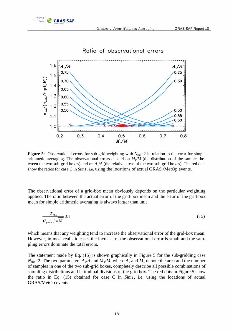
Figure 5: Observational errors for sub-grid weighting with Nsub=2 in relation to the error for simple arithmetic averaging. The observational errors depend on M1/M (the distribution of the samples be-tween the two sub-grid boxes) and on A1/A (the relative areas of the two sub-grid boxes). The red dots show the ratios for case C in Sim1, i.e. using the locations of actual GRAS /MetOp events. The observational error of a grid-box mean obviously depends on the particular weighting applied. The ratio between the actual error of the grid-box mean and the error of the grid-box mean for simple arithmetic averaging is always larger than unit

1obsp,

obs ≥Mσ

σ (15)

which means that any weighting tend to increase the observational error of the grid-box mean. However, in most realistic cases the increase of the observational error is small and the sam-pling errors dominate the total errors. The statement made by Eq. (15) is shown graphically in Figure 5 for the sub-gridding case Nsub=2. The two parameters A1/A and M1/M, where A1 and M1 denote the area and the number of samples in one of the two sub-grid boxes, completely describe all possible combinations of sampling distributions and latitudinal divisions of the grid box. The red dots in Figure 5 show the ratio in Eq. (15) obtained for case C in Sim1, i.e. using the locations of actual GRAS/MetOp events.

GRAS SAF Report 10


19

5. Spatial Distributions of RO events The spatial distribution of occultation events depends on the orbits of both the GPS satellites and the satellite carrying the RO instrument. It also depends on the observation geometry of RO instruments – the fact that it is horizon scanning rather than cross-track scanning or nadir observing. We can expect all RO missions in low-Earth orbit to share some basic spatial sam-pling characteristics. The differences depend mainly on the altitude of the RO satellite (which, amongst other things, determines the distance to the horizon) and the inclination of the orbit (which determines the precession of the orbit and how close to the poles it gets). Figures 2b and 5 provide demonstrations of the overall similarities between the spatial distri-butions of RO observations made from CHAMP and MetOp.

Figure 6: Spatial distributions of occultation events: for GRAS (upper panels) from the 3-month pe-riod June-August 2009 and for CHAMP (lower panels) from the 12-month period January-December 2002. The panels to the left show the distributions per degree of latitude, while the panels to the right show the distributions per area unit.


20

6. Conclusions

Based on the arguments in Section 2 and on the simulations in Section 3, we conclude that cosine weighting should only be used if the data are obtained from a regular latitude grid, or if the data are randomly drawn from a distribution of latitudes with a uniform probability of occurrence per degree of latitude. This is not the case with RO data. Based on the same arguments we conclude that the two-term discrete approximation – i.e. sub-gridding as formulated by Eq. (4) – of the area-weighting integral is a better alternative than cosine weighting. It is based on fewer assumptions concerning the distribution of obser-vations and, unlike cosine weighting, the sampling errors are always smaller than they are for a simple arithmetic grid-box mean (i.e. the no-weighting case).

GRAS SAF Report 10


21

References [1] Vose, R., et al., An evaluation of the time of observation bias adjustment in the U.S. Historical

Climatology Network, Geophys, Res. Lett., 30, doi:10.1029/2003GL018111, 2003. [2] Temperature Trends in the Lower Atmosphere: Steps for Understanding and Reconciling Differ-

ences. Thomas R. Karl, Susan J. Hassol, Christopher D. Miller, and William L. Murray, editors, 2006. A Report by the Climate Change Science Program and the Subcommittee on Global Change Research, Washington, DC.

[3] Foelsche, et al., An observing system simulation experiment for climate monitoring with GNSS

radio occultation data: Setup and test bed study, J. Geophys. Res., 113, doi:10.1029/2007JD009231, 2008.

[4] Foelsche, et al., Observing upper troposphere-lower stratosphere climate with radio occultation

data from the CHAMP satellite, Clim. Dyn., 31, doi:10.1007/s00382-007-0337-7, 2008. [5] Ho et al., Estimating the uncertainty of using GPS radio occultation data for climate monitoring:

Intercomparison of CHAMP refractivity climate records from 2002 to 2006 from different data centers, J. Geophys. Res., 114, doi:10.1029/2009JD011969, 2009.

[6] Steiner, et al., Atmosphere temperature change detection with GPS radio occultation 1995 to 2008,

Geophys, Res. Lett., 36, doi:10.1029/2009GL039777, 2009. [7] Steiner, et al., A multi-year comparison of lower stratospheric temperatures from CHAMP radio

occultation data with MSU/AMSU records, J. Geophys, Res., 112, doi:10.1029/2006JD008283, 2007.

GRAS SAF Reports SAF/GRAS/METO/REP/GSR/001 Mono-dimensional thinning for GPS Radio Occulation SAF/GRAS/METO/REP/GSR/002 Geodesy calculations in ROPP SAF/GRAS/METO/REP/GSR/003 ROPP minimiser – minROPP SAF/GRAS/METO/REP/GSR/004 Error function calculation in ROPP SAF/GRAS/METO/REP/GSR/005 Refractivity calculations in ROPP SAF/GRAS/METO/REP/GSR/006 Levenberg-Marquardt minimisation in ROPP SAF/GRAS/METO/REP/GSR/007 Abel integral calculations in ROPP SAF/GRAS/METO/REP/GSR/008 ROPP thinner algorithm SAF/GRAS/METO/REP/GSR/009 Refractivity coefficients used in the assimilation of GPS radio occultation measurements GRAS SAF Reports are accessible via the GRAS SAF website http://www.grassaf.org.

latitudinal binning and area-weighted averaging of ... · latitudinal binning and area-weighted...

Documents