binning in gaussian kernel regularization
TRANSCRIPT
Binning in Gaussian Kernel Regularization
Tao Shi and Bin Yu
Department of Statistics, University of California
Abstract
Gaussian kernel regularization is widely used in the machine learning literature and proven
successful in many empirical experiments. The periodic version of the Gaussian kernel reg-
ularization has been shown to be minimax rate optimal in estimating functions in any finite
order Sobolev spaces. However, for a data set with n points, the computation complexity of
the Gaussian kernel regularization method is of order O(n3).
In this paper we propose to use binning to reduce the computation of Gaussian kernel
regularization in both regression and classification. For the periodic Gaussian kernel regression,
we show that the binned estimator achieves the same minimax rates of the unbinned estimator,
but the computation is reduced to O(m3) with m as the number of bins. To achieve the
minimax rate in the k-th order Sobolev space, m needs to be in the order of O(kn1/(2k+1)),
which makes the binned estimator computation of order O(n) for k = 1 and even less for larger
k. Our simulations show that the binned estimator (binning 120 data points into 20 bins in
our simulation) provides almost the same accuracy with only 0.4% of computation time.
For classification, binning with the L2-loss Gaussian kernel regularization and the Gaussian
kernel Support Vector Machines is tested in a polar cloud detection problem. With basically the
same computation time, the L2-loss Gaussian kernel regularization on 966 bins achieves better
test classification rate (79.22%) than that (71.40%) on 966 randomly sampled data. Using the
OSU-SVM Matlab package, the SVM trained on 966 bins has a comparable test classification
rate as the SVM trained on 27,179 samples, but reduces the training time from 5.99 hours to
2.56 minutes. The SVM trained on 966 randomly selected samples has a similar training time
as and a slightly worse test classification rate than the SVM on 966 bins, but has 67% more
1

support vectors so takes 67% longer to predict on a new data point. The SVM trained on 512
cluster centers from the k-mean algorithm reports almost the same test classification rate and
a similar number of support vectors as the SVM on 512 bins, but the k-mean clustering itself
takes 375 times more computation time than binning.
KEY WORDS: Asymptotic minimax risk, Binning, Gaussian reproducing kernel, Regular-
ization, Rate of convergence, Sobolev space, Support Vector Machines.
1 Introduction
The method of regularization has been widely used in the nonparametric function estimation
problem. The problem begins with estimating a function f using data (xi, yi), i = 1, · · · , n,
from a nonparametric regression model:
yi = f(xi) + εi, i = 1, · · · , n, (1)
where xi ∈ Rd, i = 1, · · · , n, are regression inputs or predictors, yi’s are the responses,
and εi’s are i.i.d. N(0, σ2) Gaussian noises. The method of regularization takes the form of
finding f ∈ F that minimizes
L(f, data) + λJ(f) (2)
where L is an empirical loss, often taken to be the negative log-likelihood. J(f) is the
penalty functional, usually a quadratic functional corresponding to a norm or semi-norm of
a Reproducing Kernel Hilbert Space (RKHS) F . The regularization parameter λ trades off
the empirical loss with the penalty J(f). In the regression case we may take L(f,data) =∑n
i=1(yi − f(xi))2 and the penalty functional J(f) usually measures the smoothness.
In the nonparametric statistics literature, the well-known smoothing spline (cf Wahba
1990) is an example of regularization method. The reproducing kernel Hilbert space used
in smoothing spline is a Hilbert Sobolev space and the penalty J(f) =∫
[f (m)(x)]2dx is the
norm or semi-norm in the space. The reproducing kernel of the Hilbert Sobolev space was
2
nicely covered in Wahba (1990), and the commonly used cubic spline corresponds to the case
m = 2.
In the machine learning literature, Support Vector Machines (SVM) and regularization
networks, which are both regularization methods, have been used successfully in many prac-
tical applications. Smola et al (1998), Wahba (1999), and Evgeniou et al (2000) make the
connection between both methods and the methods of regularization in the Reproducing Ker-
nel Hilbert Space (RKHS). SVM uses a hinge loss function L(f, data) =∑n
i=1(1−yif(xi))+
in (2) with labels yi coded as {−1, 1} in the two-class case. The penalty functional J(f)
used in SVM is the norm of the RKHS (see Vapnik 1995 and Whaba et al 1999 for details).
One particularly popular reproducing kernel used in the machine learning literature is
the Gaussian kernel, which is defined as G(s, t) = (2π)−1/2ω−1exp((s− t)2/2ω2). Girosi et al
(1993) and Smola et al (1998) showed that the Gaussian kernel corresponds to the penalty
functional
Jg(f) =∞∑
m=0
ω2m
2mm!
∫ ∞
−∞[f (m)(x)]2dx. (3)
Smola et al (1998) also introduced the periodic Gaussian reproducing kernel for estimating
2π-periodic functions in (−π, π] as the kernel corresponding to penalty functional
Jpg(f) =∞∑
m=0
ω2m
2mm!
∫ π
−π
[f (m)(x)]2dx (4)
Using the equivalence between the nonparametric regression and Gaussian white noise
model shown in Brown and Low (1996), Lin and Brown (2004) showed asymptotic proper-
ties of the regularization using a periodic Gaussian kernel. The periodic Gaussian kernel
regularization is rate optimal in estimating functions in all finite order Sobolev spaces. It is
also asymptotically minimax for estimating functions in the infinite order Sobolev Space and
the space of analytic functions. These asymptotic results on the periodic Gaussian kernel
gave a partial explanation of the success of the Gaussian reproducing kernel in practice. In
section 2, we describe the periodic Gaussian kernel regularization in nonparametric regres-
sion setup and review the asymptotic results, which will be compared to the binning results
3

in section 4. Although having good statistical properties, the Gaussian kernel regularization
method is computationally very expensive, usually of order O(n3) on n data points. It is
computationally infeasible when n is too large.
In this paper, motivated by the application of binning technique in nonparametric re-
gression (cf Hall et al 1998), we study the effect of binning in the periodic Gaussian kernel
regularization. We first show the eigen structure of the periodic Gaussian kernel in the finite
sample case, then the eigen structure is used to prove the asymptotic minimax rates of the
binned periodic Gaussian kernel regularization estimator. The results on the kernel matrix
are given in section 3.
In section 4, we show the binned estimator achieves the same minimax rates of the
unbinned estimator, while the computation is reduced to O(m3) with m as the number of
bins. To achieve the minimax rate in the k-th order Sobolev space, m needs to be in the
order of O(kn1/(2k+1)), which makes the binned estimator computation to be O(n) for k = 1
and even less for larger k. For estimating functions in the Sobolev space of infinite order,
the number of bins m only needs to be in the order of O(√
log(n)) to achieve the minimax
risk. For the simple average binning, the optimal regularization parameter λB for binned
data has a simple relationship with the optimal λ for the unbinned data, λB ≈ mλ/n and ω
stays the same. In practice, choosing parameters (λB, ω) by Mallow’s Cp statistics achieves
the asymptotic rates.
In section 5, experiments are carried out to assess the accuracy and the computation
reduction of the binning scheme in regression and classification problems. We first run
simulations to test binning periodic Gaussian kernel Regularization in the nonparametric
regression setup. Four periodic functions with different order of smoothness are used the
simulation. Comparing to the unbinned estimators on 120 data points, the binned estimators
(6 data in each bin) provide the same accuracy, but requires only 0.4% of computation.
For classification, binning on the L2-loss Gaussian kernel regularization and the Gaussian
kernel Support Vector Machines are tested in a polar cloud detection problem. With the
4

same computation time, the L2-loss Gaussian kernel regularization on 966 bins achieves
better accuracy (79.22%) than that (71.40%) on 966 randomly sampled data. Using the
OSU-SVM Matlab package, the SVM trained on 966 bins has a comparable test classification
rate as the SVM trained on 27,179 samples, and reduces the training time from 5.99 hours
to 2.56 minutes. The SVM trained on 966 randomly selected samples has a similar training
time as and a slightly worse test classification rate than the SVM on 966 bins, but has 67%
more support vectors so takes 67% longer to predict on a new data point.
Compare to k-mean clustering, another possible SVM training sample-size reduction
scheme proposed in Feng and Mangasarian (2001), binning is much faster than k-mean
clustering. The SVM trained on 512 cluster centers from the k-mean algorithm reports
almost the same test classification rate and a similar number of support vectors as the SVM
on 512 bins, but the k-mean clustering itself takes 375 times more computation time than
binning. Therefore, for both the regression and classification in practice, binning Gaussian
kernel regularization reduces the computation and keeps the estimation or classification
accuracy. Section 6 contains summaries and discussions.
2 Periodic Gaussian Kernel Regularization
Lin and Brown (2004) studied the asymptotic properties of the periodic Gaussian kernel reg-
ularization in estimating 2π-periodic functions on (−π, π] in three different function spaces.
Using the asymptotic equivalence between the nonparametric regression and the Gaussian
white noise model (see Brown and Low 1996), the asymptotic properties of the periodic
Gaussian kernel regularization are proved in the Gaussian white noise model. In this sec-
tion, we introduce the periodic Gaussian regularization and review the asymptotic results
by Lin and Brown (2004) in the nonparametric regression setting.
5

2.1 Nonparametric Regression
In this paper, we consider estimating periodic function on (0, 1] using periodic Gaussian
regularization. With data (xi, yi), i = 1, · · · , n, observed from model (1) at equal space
designed points xi’s, the method of periodic Gaussian kernel regularization with L2 loss
estimates f by a periodic function fλ that minimizes
n∑i=1
(yi − f(xi))2 + λJpg(f) (5)
where Jpg(f) is the norm of the corresponding RKHS FK of the periodic Gaussian kernel
(Smola et al, 1998)
K(s, t) = 2∞∑
l=0
exp(−l2ω2/2) cos(2πl(s− t)). (6)
The theory of reproducing kernel Hilbert space guarantees that the solution to (5) over
FK falls in the finite dimensional space spanned by {K(xi, ·), i = 1, · · · , n} (see Wahba
1990 for an introduction to the theory of reproducing kernels). Therefore, we can write the
solution to (5) as f(x) =∑n
i=1 ciK(xi, x) and the minimization problem can then be solved
in this finite dimensional space. Using the finite expression, (5) becomes
minc
[(y −G(n)c)T (y −G(n)c) + λcT G(n)c], (7)
where y = (y1, · · · , yn)T , c = (c1, · · · , cn)T , and G(n) as a n × n matrix K(xi, xj). The
solution is c = (G(n) + λI)−1y with I being a n × n identity matrix. The fitted values are
y = G(n)c = G(n)(G(n) + λI)−1y , Sy, which is a linear estimator. The asymptotic risk of
this estimator is shown in the next section.
2.2 Asymptotic Properties
We briefly review the asymptotic results shown in Lin and Brown (2004) in this section and
compare them to the binned estimators in section 4. The asymptotic risk of periodic Gaussian
6

regularization is studied in estimating periodic function from three types of function spaces:
spaces of Sobolev ellipsoid of finite order, ellipsoid spaces of analytic functions, and Sobolev
spaces of infinite order, which are defined as follows. (Instead of working with 2π-periodic
functions on (−π, π], we study periodic functions on (0,1] in this paper.)
The first type of function space, k-th order Sobolev ellipsoid Hk(Q), is defined as
Hk(Q) = {f ∈ L2(0, 1) : f is periodic,
∫ 1
0
[f(t)]2 + [f (k)(t)]2dt ≤ Q}. (8)
It has an alternative definition in the Fourier space as:
Hk(Q) = {f : f(t) =∞∑
l=0
θlφl(t),∞∑
l=0
γlθ2l ≤ Q, γ0 = 1, γ2l−1 = γ2l = l2k + 1}, (9)
where φ0(t) = 1, φ2l−1(t) =√
2 sin(2πlt), φ2l(t) =√
2 cos(2πlt) are the classical trigonometric
basis in L2(0, 1) and θl =∫ 1
0f(t)φl(t)dt is the corresponding Fourier coefficient.
The second function space being considered is the ellipsoid space of analytic functions
Aα(Q), which corresponds to (9) with the exponentially increasing sequence γl = exp(αl).
The third function space is the infinite order Sobolev space H∞ω (Q), which corresponds to
(9) with the sequence ρ0 = 1 and γ2l−1 = γ2l = el2ω2/2. Note that the penalty functional Jpg
of periodic Gaussian kernel regularization is the norm of H∞ω (Q).
The asymptotic risk of y is determined by the tradeoff between the variance and the bias.
The asymptotic variance of y = G(n)c = G(n)(G(n) + λI)−1y depends only on λ and ω, while
G(n) denotes matrix K(xi, xj). In the mean time, the asymptotic bias depends not only on λ
and ω, but also on the function f itself. Lin and Brown (2004) proved the following lemma
using the equivalence between the nonparametric regression and the Gaussian white noise
model (Brown an Law 1996).
Lemma 1 (Lin and Brown 2004) In nonparametric regression, the solution y to the periodic
Gaussian kernel regularization problem (7) has an asymptotic variance:
1
n
∑var(yi) = (1/n)
∑(1 + λβl)
−2 ∼ 2√
2ω−1n−1(− log λ)1/2, (10)
7

for βl = exp(l2ω2/2) as λ goes to zero. The asymptotic bias is:
1
n
∑bias2(yl) ∼
∑λ2β2
l (1 + λβl)−2θ2
l . (11)
when estimating function f(t) =∑∞
l=0 θlφl(t).
Based on (10) and (11), following asymptotic results about the periodic Gaussian kernel
regularization are shown.
Lemma 2 (Lin and Brown 2004) For estimating functions in the k-th order Sobolev space
Hk(Q), the periodic Gaussian kernel regularization has a minimax risk:
(2k + 1)k−2k/(2k+1)Q1/(2k+1)n−2k/(2k+1),
achieved when log(n/λ)/ω2 ∼ (knQ)2/(2k+1)/2. The minimax rate for estimating functions
in Aα(Q) is
2n−1α−1(log n),
and the rate is
2√
2ω−1n−1(log n)1/2
for estimating functions in H∞ω (Q).
It is well known that the asymptotic minimax risk over Hk(Q) is [2k/(k+1)]2k/(2k+1)(2k+
1)1/(2k+1)Q1/(2k+1)n−2k/(2k+1). If we calculate the efficiency of the periodic Gaussian kernel
regularization in terms of sample sizes need to achieve the same risk, the efficiency goes to
one when the function gets smoother. Therefore, the estimator is rate optimal in this case.
For estimating functions in Aα(Q) and H∞ω (Q), the periodic Gaussian kernel regularization
achieves the minimax risk (see Johnstone 1998 for the proof of minimax risk in Aα(Q)).
These asymptotic rates in Lemma 2 are compared with the binning results in section 4.
8

3 The Eigen Structure of the Projection Matrix
Instead of working with the Gaussian white noise model, we directly prove Lin and Brown’s
asymptotic results in the nonparametric regression model in this section. Although the
results stated in section 2.2 are proved more easily in the Gaussian white noise model than
in the regression model, knowing the eigen structure of the projection matrix S (defined as
y = G(n)(G(n) + λI)−1y , Sy in section 2.1) helps us understand the binned estimators in
section 4. To study the variance-bias trade-off of the periodic Gaussian regularization, we
first derive the eigen-values and eigen-vectors of G(n) = K(xi, xj) and make the connections
between them to the functional eigen-values and eigen-functions of the reproducing kernel
K(·, ·).
For a general reproducing kernel R(·, ·) that satisfies∫ ∫
R2(x, y)dxdy < ∞, there exist
an orthonormal sequence of eigen-functions φ1, φ2, · · · , and eigen-values ρ1 ≥ ρ2 ≥ · · · ≥ 0,
with ∫ b
a
R(s, t)φl(s)ds = ρlφ(t), l = 1, 2, ... (12)
and R(s, t) =∑∞
l=1 ρlφl(s)φl(t). When equally spaced points x1, · · · , xn are taken in (a, b], we
get a Gram matrix R(n)i,j = R(xi, xj). The eigen-vectors and eigen-values of R(n) are defined
as a sequence of orthonormal n by 1 vectors v1, · · ·, vn and values d1 ≥ · · · ≥> 0dn, that
satisfy
R(n)V(n)l = d
(n)l V
(n)l , l = 1, 2, ...n (13)
and R(n) =∑n
l=1 d(n)l V
(n)l V
(n)T
l . The eigen-values d(n)l have limits: limn→∞d
(n)l (b− a)/n = ρl
(c.f. Williams and Seeger 2000).
On (0, 1], the eigen-functions of the periodic Gaussian kernel K are the classical trigono-
metric basis functions φ0(t) = 1, φ2l−1(t) =√
2 sin(2πlt), φ2l(t) =√
2 cos(2πlt), with the
corresponding eigen-values ρ0 = 1 and ρ2l−1 = ρ2l = exp(−l2ω2/2) (For notation simplicity,
the labels of eigen-values and eigen-functions start from 0 instead of 1). It is straightforward
9

to see the eigen function decomposition when we rewrite K(s, t) as:
K(s, t) = 2∞∑
l=0
exp(−l2ω2/2) cos(2πl(s− t))
=∞∑
l=0
e−l2ω2/2[√
2 sin(2πls)√
2 sin(2πlt) +√
2 cos(2πls)√
2 cos(2πlt)]
=∞∑
l=0
ρlφl(s)φl(t)
where φl(t)’s are orthonormal on (0, 1]. When n equally spaced data points are taken over
(0, 1], such as xi = − 12n
+ in, the Gram matrix G(n) = K(xi, xj) has the following property:
Theorem 1 The Gram matrix G(n) = K(xi, xj) at equal-spaced data points x1, · · · , xn over
(0, 1] has eigen-vectors V(n)0 , V
(n)1 , · · · , V (n)
n−1 (indexed from 0 to n− 1):
V(n)0 =
√1/n(1, · · · , 1)T =
√1/n(φ0(x1), · · · , φ0(xn))T ,
V(n)l =
√2/n(sin(2πhx1), · · · , sin(2πhxn))T =
√1/n(φl(x1), · · · , φl(xn))T , for odd l,
V(n)l =
√2/n(cos(2πhx1), · · · , cos(2πhxn))T =
√1/n(φl(x1), · · · , φl(xn))T for even l,
where h = d(l + 1)/2e, l = 1, · · · , n − 1, and dae stands for the integer part of a. Their
corresponding eigen-values are:
d(n)0 = 2n
∞∑
k=0
(−1)kρ2kn
d(n)l = n{ρl +
∞∑
k=1
(−1)k[ρkn+h + (−1)l−2hρkn−h]}
The proof is given in the appendix. This theorem shows that the eigen-vector V(n)l is exactly
the evaluation of eigen-function φl(·) at x1, · · · , xn, scaled by√
(1/n). It is worth to point
out that this exact relationship between eigen-functions and eigen-vectors does not generally
hold for other kernels and data distributions. For general kernels and data distributions, one
can only prove that the eigen-vectors converges to the corresponding eigen-functions as the
10

sample size goes to infinity. Therefore, the eigen-vectors can not be explicitly written out in
the finite sample case.
With the eigen decomposition of G(n), we now study the variance-bias trade-off of the pe-
riodic Gaussian kernel regularization. Using the matrix notation, let V (n) , (V(n)0 , · · · , V (n)
n−1)
and let D(n) , diag(d(n)0 , · · · , d(n)
n−1) be an n by n diagonal matrix , then G(n) = V (n)D(n)V (n)T .
For the variance term, recall S = G(n)(G(n) + λI)−1, we have S = V (n)diag(d(n)l
d(n)l +λ
)V (n)T .
Therefore, the variance term is:
1
n
∑var(yi) =
1
ntrace(ST S) =
1
n
n−1∑
l=0
(d
(n)l
d(n)l + λ
)2 =1
n
n−1∑
l=0
(d
(n)l /n
d(n)l /n + λ/n
)2.
Since limn→∞d(n)l /n = ρl for l > 0 and ρl = 1/βl, we get
1
n
∑var(yi) ∼ 1
n
∑(
ρl
ρl + (λ/n))2 =
1
n
∑(1 + βl(
λ
n))−2,
which is the same as the asymptotic variance shown in (10).
For the bias term, we expand f(t) as f(t) =∑∞
l=0 θlφl(t). Using the relationship between
V (n) and φ(·) in Theorem 1, we can write vector F = (f(x1), · · · , f(xn))T as
F =n−1∑
l=0
Θ(n)l V
(n)l = V (n)Θ(n),
where
Θ(n)0 =
√n
∞∑
k=0
(−1)kθ2kn,
Θ(n)l =
√n{θl +
∞∑
k=1
(−1)k[θkn+h + (−1)l−2hθkn−h]},
for 1 ≤ l ≤ n− 1 and h = d(l + 1)/2e. Thus, the bias term is written as:
1
n
∑Bias2(yi) =
1
n((S − I)F )T ((S − I)F )
=1
n(V (n)diag(
λ
d(n)l + λ
)V (n)T F )T (V (n)diag(λ
d(n)l + λ
)V (n)T F )
=1
n
n−1∑
l=0
(Θ
(n)l λ
d(n)l + λ
)2 =1
n
n−1∑
l=0
n(Θ
(n)l√n
)2(λ/n
d(n)l /n + λ/n
)2
11

∼∑
θ2l (
λ/n
ρl + λ/n)2
=∑
θ2l (
βlλ/n
1 + βlλ/n)2,
since limn→∞Θ(n)l /
√n = θl, limn→∞d
(n)l /n = ρl, and ρl = 1/βl.
Both the variance and bias are the same as in Lemma 1 derived by using the Gaussian
white noise model in Lin and Brown (2004). Although it is easier to prove Lemma 1 and 2
in the Gaussian white noise model than through the eigen expansion derived above, binned
estimators in the nonparametric regression setup do not directly convert to the Gaussian
white noise model. Therefore, the eigen expansion is used to prove the asymptotic properties
of binning the periodic Gaussian kernel regularization in the next section.
4 Binning Periodic Gaussian Kernel Regularization
Although the periodic Gaussian regularization method has good asymptotic properties, the
computation of the estimator y = G(n)(G(n) + λI)−1y is very expensive, taking O(n3) to
invert the n by n matrix G(n) +λI. When the sample size gets large, the computation is not
even feasible. In nonparametric regression estimation, Hall et al (1998) studied the binning
technique. In this section, we use the explicit eigen structure of the periodic Gaussian
kernel to study the effect of binning on the asymptotic properties of periodic Gaussian
regularization.
4.1 Simple Binning Scheme
Let us take equally spaced n data points in (0, 1], say xi = − 12n
+ in. Without loss of
generality, we assume the number of design point n equals m × p, while m is the number
of bins and p is number of data points in each bin. Using equally spaced binning scheme,
let us denote the centers of bins as xj = (x(j−1)×p+1 + · · ·+ x(j−1)×p+p)/p and the average of
12

observations in each bin as yj = (y(j−1)×p+1 + · · ·+ y(j−1)×p+p)/p, for j = 1, · · · ,m. When we
apply the periodic Gaussian regularization to the binned data, the estimated function is in
the form of f(x) =∑m
j=1 cjK(x, xj), where c is the solution of
minc
(y −G(m)c)T (y −G(m)c) + λBcT G(m)c, (14)
with G(m)i,j = K(xi, xj), y = (y1, · · · , ym) and λB as the regularization parameter. Similar to
the estimator derived in section 2.1, the solution of (14) is c = (G(m) + λBI)−1y. With this
explicit form of the binned estimator, we study its asymptotic properties next. Let
B(m,n) =
m/n · · · m/n 0 · · · · · · 0
0 · · · 0 m/n · · · m/n 0 · · · 0
· · · · · ·0 · · · · · · 0 m/n · · · m/n
m×n
. (15)
The binned estimator can be written as y = G(n,m)(G(m) + λBI)−1B(m,n)y = SBy with
G(n,m)i,j = K(xi, xj) being a n by m matrix. From this expression, it is straightforward to see
that the computation is reduce to O(m3) since the matrix inversion is taken on an m by m
matrix now. The additional computation for binning the data itself is around O(n), which
is trivial comparing to the matrix inversion computation O(n3).
Using this matrix expression, The variance of the estimator can be written as:
1
n
∑var(yi) =
1
ntrace(ST
BSB) =1
ntrace(SBST
B) (16)
Based on the following proposition, the variance term can be explicitly written out using the
eigen-decomposition of SB.
Proposition 1 Suppose n = mp, xi = − 12n
+ in, and xj = (x(j−1)×p+1 + · · ·+ x(j−1)×p+p)/p.
The eigen-vectors V (m)of G(m) and the eigen-vectors V (n) of G(n) satisfy
G(n,m)V(m)k = d
(m)k
√n
mV
(n)k for k = 0, 1, · · · ,m.
13

The proof is provided in the appendix. This proposition shows that the eigen-vector of G(m)
are projected to the corresponding eigen-vector of G(n) by the matrix G(n,m) (Unfortunately,
this property does not hold for general kernels). Following this relationship, the asymptotic
variance of the binned estimator is provided in the following theorem:
Theorem 2 The asymptotic variance of the binned estimator y = G(n,m)(G(m)+λBI)−1B(m,n)y
in the equally spaced binning scheme is:
1
n
∑var(yi) ∼ 1
n
∑(1 +
βlλB
m)−2 ∼ 2
√2w−1n−1(− log(λB/m))1/2, (17)
as m →∞, n →∞ and λB → 0. The expression is the same as the asymptotic variance of
the original estimator when λB = mλ/n.
See the proof in the appendix. Now we focus on the bias term, which depends not only on
the projection operation, but also on the smoothness of the underline function f itself. We
have the following theorem for the bias term:
Theorem 3 In the equally spaced binning scheme, as m → ∞, n → ∞, m/n → 0 and
λB → 0, the bias of the binned estimator is:
1
n
∑Bias2(yi) ∼
m−1∑j=0
θ2j (
βjλB/m
1 + βjλB/m)2 +
∞∑j=m
θj2. (18)
when estimating function f(t) =∑∞
l=0 θlφl(t).
The theorem is proved in the appendix. With the asymptotic variance and bias obtained, we
show in the next section that the asymptotic minimax rates of the periodic Gaussian kernel
regularization are kept after binning the data.
4.2 Asymptotic Rates of Binned Estimators
In this section, we study the asymptotic rates of the binned periodic Gaussian kernel regu-
larization in estimating functions in spaces defined in section 2.2. We start with the infinite
14

order Sobolev space. As shown in the next theorem, the binned estimator also achieves the
minimax rate as the original estimator does in this space.
Theorem 4 The minimax rate of the binned estimator y = G(n,m)(G(m) + λBI)−1B(m,n)y
for estimating functions in the infinite order Sobolev space H∞w (Q) is:
min maxθ∈H∞
w (Q)E[
1
n(y − y)T (y − y)] ∼ 2
√2w−1n−1(log n)1/2,
which is the same rate of the unbinned estimator. This rate is achieved when m/n → 0, and
m is large enough so that w2m2/2 > log(4m/λB). The parameter λB = λB(n,m) satisfies
log(m/λB) ∼ log n, λB/m = o(n−1(log n)1/2). This leads m to be in an order of O(√
log(n)).
Proof: As shown in Theorem 3, the bias of the binned estimator is:
1
n
∑Bias2(yi) ∼
m−1∑
l=0
θ2l (
βlλB/m
1 + βlλB/m)2 +
∞∑
l=m
θl2
≤ λB
4m
m−1∑
l=0
βlθ2l +
∞∑
l=m
θ2l
≤ λB
4m
∞∑
l=0
βlθ2l (when
λBβm
4m> 1)
≤ λB
4mQ,
and λBβm/4m > 1 is satisfied as w2m2/2 > log(4m/λB). Then the asymptotic risk is
1
nE[(y − y)T (y − y)] ≤ 1
n
∑(1 +
βlλB
m)−2 +
λB
4mQ ∼ 2
√2w−1n−1(log n)1/2,
when log(m/λB) ∼ log n and λB/m = o(n−1(log n)1/2). ¤
The theorem shows the binned estimator achieves the same asymptotic rate of the original
estimator when m is the order of O(√
log(n)). Therefore, the computation complexity of
the binned estimator is around O(log n)3/2. In practice, we do not expect m can be as small
as in this order, since this type of function is not realistic in common applications. Next we
study the case of estimating functions in the Sobolev space Hk(Q) with finite order k.
15

Theorem 5 The minimax rate of the binned estimator y = G(n,m)(G(m) + λBI)−1B(m,n)y
for estimating functions in the k-th order Sobolev space Hk(Q) is:
minm,w,λB
maxθ∈Hk(Q)
1
nE[(y − y)T (y − y)] ∼ (2k + 1)k−2k/(2k+1)Q1/(2k+1)n−2k/(2k+1),
which is the same rate of the unbinned estimator. This rate is achieved when: m/n → 0 and
m is large so that m >√
2w−1(− log(λB/m))1/2. The parameter λB = λB(n,m, w) satisfies
log(m/λB)/w2 ∼ (knQ)2/(2k+1)/2. The condition leads m to be in an order of O(kn1/(2k+1)).
Proof: We first study the bias term, let λm = λB/m
B(m,w, λm) = maxθ∈Hk(Q)
m−1∑
l=0
θ2l (
βlλm
1 + βlλm
)2 +∞∑
l=m
θl2
= maxθ∈Hk(Q)
m−1∑
l=0
(1 + β−1l λ−1
m )−2ρ−1l (ρlθ
2l ) +
∞∑
l=m
ρ−1l (ρlθ
2l )
Here ρ2l−1 = ρ2l = 1 + l2k are the coefficients in the definition (8) of Sobolev ellipsoid
Hk(Q). The maximum is achieved by putting all mass Q at the l term that maximizes∑m−1
l=0 (1 + β−1l λ−1
m )−2ρ−1l +
∑∞l=m ρ−1
l . First let us find the maximizer of
Aλm(x) = [1 + λ−1m exp(−x2w2/2)]−2(1 + x2k)−1 over x ≥ 0
As shown in Lin and Brown (2004), the maximizer x0 satisfies x20w
2/2 ∼ (− log λm) and the
maximum Aλm(x0) ∼ x−2k0 ∼ 2−kw2k(− log λm)−k. When m > x0 and m ≥ √
2w−1(− log λm)1/2,
we have (1+m2k)−1 < 2−kw2k(− log λm)−k. Therefore, the maximum value of B(m,w, λm) ∼Q2−kw2k(− log λm)−k. Thus we have the following:
maxθ∈Hk(Q)
1
nE[(y − y)T (y − y)] ∼ Q2−kw2k(− log λm)−k + 2
√2w−1n−1(− log λm)1/2.
This asymptotic rate (2k +1)k−2k/(2k+1)Q1/(2k+1)n−2k/(2k+1) is achieved when the parameters
satisfy log(m/λB)/w2 ∼ (knQ)2/(2k+1)/2 and m >√
2w−1(− log(λB/m))1/2. ¤
The theorem shows the binned estimator achieves the same minimax rate of the original
estimator in the finite order Sobolev space. The same result also holds in the ellipsoid Aα(Q)
16

of analytic functions but we would not prove it here. Comparing the order of smallest m
needed to achieve the optimal rates for estimating functions with different order of smooth-
ness, we find that the smoother functions require a smaller number of bins. For instance,
the optimal rate of estimating a function in the k-th order Sobolev space can be achieved by
binning the data into m = O(kn1/(2k+1)) number of bins. The number of bins m decreases
as k increases. Binning reduces the computation from O(n3) to O(m3) = O(n) for k = 1, to
O(n3/5) for k = 2, and even less for larger k values.
5 Experiments
Simulations and real data experiments are conducted in this section to study the effect
of binning in regressions and classifications. We first use simulations to study binning in
estimating periodic functions in the nonparametric regression setup. The results show that
the accuracy of binned estimators are no worse than the original estimators when function
are smooth enough. Meanwhile, the computation is reduced to 0.4% of the computation
original estimator, when the original 120 data points in binned into 20 bins.
For classification, we test the binning idea on a problem raised in a polar cloud detection
problem (cf Shi et al 2004). The L2 loss and hinge loss functions are both tested in this ex-
periment. In both cases, the binned classifier provide competitive results to classifiers trained
from full data. Furthermore, the computation time is significantly reduced by binning. As
an illustration, the time for training SVM on 966 bins is 2.56 minutes, only 0.071% of 5.99
hours that is used to train SVM on 27179 samples, which provide slightly better accuracy
than the SVM on 966 bins.
17

0 0.2 0.4 0.6 0.8 10
0.2
0.4
0.6
0.8
1
x
f 1(x
)
0 0.2 0.4 0.6 0.8 1−0.4
−0.3
−0.2
−0.1
0
0.1
0.2
0.3
x
f 2(x
)
0 0.2 0.4 0.6 0.8 10.3
0.4
0.5
0.6
0.7
0.8
0.9
1
x
f 3(x
)
0 0.2 0.4 0.6 0.8 1−5
0
5
10
15
x
f 4(x
)
0 0.2 0.4 0.6 0.8 1−4
−3
−2
−1
0
1
2
3
x
f 1(x
) +
ε
0 0.2 0.4 0.6 0.8 1−3
−2
−1
0
1
2
3
4
x
f 2(x
) +
ε
0 0.2 0.4 0.6 0.8 1−2
−1
0
1
2
3
4
x
f 3(x
) +
ε
0 0.2 0.4 0.6 0.8 1−10
−5
0
5
10
15
x
f 4(x
) +
ε
Figure 1: Regression functions and data used in the simulations.
5.1 Non-parametric Regression
Data are simulated from the regression model (1) with noise N(0, 1), using four periodic
functions on (0, 1] with different order of smoothness.
f1(x) = sin2(2πx)1(x≤1/2)
f2(x) = −x + 2(x− 1/4)1(x≥1/4) + 2(−x + 3/4)1(x≥3/4)
f3(x) = 1/(2− sin(2πx))
f4(x) = 2 + sin(2πx) + 2 cos(2πx) + 3 sin2(2πx) + 4 cos3(2πx) + 5 sin3(2πx)
The plots of the functions are given the left of Figure 1 and the data are plotted at the
right. The first function has a second order of smoothness. The second function has the first
order of smoothness. The third function is infinitely smooth. The fourth function is even
smoother: it has a Fourier series that only contains finitely many terms. In our simulation,
the sample size n is set to 120 and the number of bins are m = 60, 40, 30, 24, 20, 15, 12,
with corresponding numbers in each bin as p = 2, 3, 4, 5, 6, 8, 10. All simulations are done in
Matlab 6.
18

1 2 3 4 5 6 7 8 9 100.04
0.05
0.06
0.07
0.08
0.09
0.1
0.11
0.12
Number of points in each bin
Resid
ual S
um
Square
Func 1Func 2Func 3Func 4
1 2 3 4 5 6 7 8 9 100.04
0.05
0.06
0.07
0.08
0.09
0.1
0.11
0.12
Number of points in each bin
Resid
ual S
um
Square
Func 1Func 2Func 3Func 4
Figure 2: Mean square errors of the binned estimators v.s the number of data points in each
bin. Left: Binned Periodic Gaussian kernel regularization; Right: Binned Gaussian kernel
regularization. In both plots, unbinned estimators are those with 1 data in each bin.
The computation of the periodic Gaussian regularization is sketched as follows. We
follow Lin and Brown (2004) to approximate the periodic Gaussian kernel defined in (6). A
Gaussian kernel G(s, t) = (2π)−1/2ω−1exp((s − t)2/2ω2) is used to approximate K(s, t). It
is shown in Willamson et al (2001) that K(s, t) =∑∞
k=−∞ G((s − t − 2kπ)/2π). Actually
GJ(s, t) =∑J
k=−J G((s− t− 2kπ)/2π) for J = 1 is already a good approximation to K(s, t)
with
0 < K(s, t)−G1(s, t) < 2.1× 10⁻²⁰, ∀(s− t) ∈ (0, 1] for w ≤ 1.
Therefore, we use G1(s, t) as an easily computable proxy of K(s, t) in the simulation.
Over the data generated from the regression model (1) on the four functions considered,
we compare the mean squared errors of the binned estimator and the original estimator. For
periodic Gaussian kernel regularization, we search over w = 0.3k1 − 0.1 for k1 = 1, · · · , 10;
and λ = exp(−0.4k2 + 7), for k2 = 1, · · · , 50. Then we compute the binned estimator for
the number data in each bin p as 2, 3, 4, 5, 6, 8, 10 separately, The parameters are set to be
ω and λB = mλ/n. In both cases, we use the minimal point of Mallow’s Cp to choose the
parameter (w, λB).
19

The simulation runs 300 times. The left panel of Figure 2 shows the averaged mean
squared errors against the number of data points in each bin for the four functions (with
the unbinned estimators shown as those with one data in each bin in the plot). In most of
the cases, the average errors of binned estimators are not significantly higher than those the
original estimators, while the computation is reduced from O(1203) to O(m3). For example,
let us consider the estimator using 6 data points in each bin (m=20). The standard error (not
shown in the plot) of the average errors are computed and two sample t tests are conducted
to compare the binned estimator to the original estimator. For all four functions, the p-
values are all larger than 0.1, which says no significant loss of accuracy by binning the data
to 20 bins in this experiment. In the mean time, the computation complexity is reduced to
O(203), 0.4% of O(1203) on full data.
In our experiment, the periodic Gaussian kernel is replaced by a Gaussian kernel, which
is most common in practice. We repeat the same experiments again and get the average
mean square errors plotted in the right panel of Figure 2. The errors from using the Gaussian
kernel are generally higher than those from the periodic Gaussian kernel, since the Gaussian
kernel does not take in account of the fact that our functions are periodic. However, the
binned estimators have almost the same accuracy as the unbinned ones when there are
enough number (say 24) of bins in this simulation. The computation reduction of Gaussian
kernel is the same as in the periodic Gaussian case.
5.2 Cloud Detection over Snow and Ice Covered Surface
In this section, we test binning in a real classification problem using Gaussian kernel regu-
larization. By reducing the variance, binning the data is expected to keep the classification
accuracy as well as relieving the computation burden even in classification. Here we illustrate
the effect of binning using a polar cloud detection problem arising in atmospheric science.
In polar regions, detecting clouds using satellite remote sensing data is difficult, because the
surface is covered by snow and ice that have similar reflecting signatures as clouds. In Shi
20
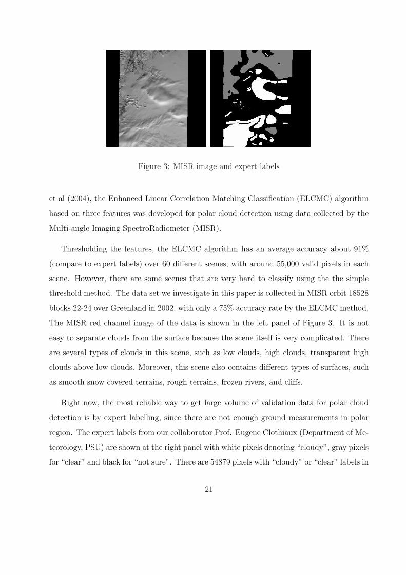
Figure 3: MISR image and expert labels
et al (2004), the Enhanced Linear Correlation Matching Classification (ELCMC) algorithm
based on three features was developed for polar cloud detection using data collected by the
Multi-angle Imaging SpectroRadiometer (MISR).
Thresholding the features, the ELCMC algorithm has an average accuracy about 91%
(compare to expert labels) over 60 different scenes, with around 55,000 valid pixels in each
scene. However, there are some scenes that are very hard to classify using the the simple
threshold method. The data set we investigate in this paper is collected in MISR orbit 18528
blocks 22-24 over Greenland in 2002, with only a 75% accuracy rate by the ELCMC method.
The MISR red channel image of the data is shown in the left panel of Figure 3. It is not
easy to separate clouds from the surface because the scene itself is very complicated. There
are several types of clouds in this scene, such as low clouds, high clouds, transparent high
clouds above low clouds. Moreover, this scene also contains different types of surfaces, such
as smooth snow covered terrains, rough terrains, frozen rivers, and cliffs.
Right now, the most reliable way to get large volume of validation data for polar cloud
detection is by expert labelling, since there are not enough ground measurements in polar
region. The expert labels from our collaborator Prof. Eugene Clothiaux (Department of Me-
teorology, PSU) are shown at the right panel with white pixels denoting “cloudy”, gray pixels
for “clear” and black for “not sure”. There are 54879 pixels with “cloudy” or “clear” labels in
21

this scene and we use half of these labels for training and half for testing different classifiers.
Each pixels is associated with a three dimensional vector X = (log(SD), CORR, NDAI),
computed from the original MISR data as described in Shi et al (2004). Hence we build and
test classifiers based on these three features.
We test binning on the Gaussian kernel regularization with two different type of loss
functions. One is the L2 loss function as we studied in this paper, and the other is the
hinge loss function corresponding to the Support Vector Machines. In both case, we binned
the data based on the empirical marginal distribution of the three predictors. For each
predictor, we found the 10%, 20%, · · ·, 90% percentiles of the empirical distribution and
these percentiles serve are the split points for each predictor. Therefore, we get 1000 bins in
the three dimensional space. In those bins, 966 of them contain data and 34 are empty. Thus,
the 966 bin centers are our binned data in the experiments. The computation is carried out
in Matlab 6 on a desktop computer with a Pentium 4 2.4GHz CPU and 512M memory.
5.2.1 Binning on Gaussian Kernel Regularization with L2 loss
The Gaussian kernel regularization with the L2 loss function is tested with three different
setups for training data. The first setup is random sampling a small proportion of data
as training data and train classification over them. This is the common approach to deal
with large data sets and it serves as a baseline for our comparison. In the second setup, the
bin centers and the majority vote of the labels in each bin are used as training data and
responses. Thus, each bin center is treated as one data point in this case. In the last setup,
the training data and labels are the bin centers and the proportion of 1’s in each bin. To
reflect the fact that different bins may have different number of data points, we also give a
weight to each bin center in the loss function in the last setup. In all there setups, a half of
the 54879 data points are left out for choosing the best parameters ω and λ.
In the first setup, we randomly sample 966 data points from the full data (54879 data
points) and use the corresponding label y (0 and 1) to train the classifier y = Kω(Kω+λI)−1y.
22

random sample size 966 GKR-L2 GKR-L2 on 966 bin
GKR-L2 Bagged GKR-L2 996 bin centers centers with fuzzy labels
Accuracy 71.40% * 77.77% 75.86% 79.22%
Comp Time 81× 26.24 81× 21× 26.24 3.87+ 81× 26.24 3.87 + 81× 26.24
(seconds) = 35.42 minutes = 12.40 hours = 35.48 minutes = 35.48 minutes
Table 1: Binning L2 Gaussian kernel regularization for cloud detection. Note: * The average
accuracy of 21 runs.
The predicted labels are set to be the indicator function I(y > 0.5). Cross-validation is
performed to chose the parameters (ω, λ) from ω = 0.8+(i−5)×0.05 and λ = .1+(j−5)×0.005 for i, j = 1, · · · , 9. For each (ω, λ) pair, this procedure is repeated for 21 times and the
average classification rate is reported. The best average classification rate is 71.40% (with
SE 0.43%). With the classification results from the 21 runs, we also take the majority vote
over the results to build a “bagged” classifier, which improve the accuracy to 77.77%. As
discussed in Breiman (1996) and Buhlmann and Yu (2002), Bagging reduces the classification
error by reducing the variance.
In the second setup, the 966 bin centers are used as training data. Cross-validation is
carried out to find the best parameters (ω, λ) over the same range as in the first setup. The
classifier is then applied to the full data to get an accuracy rate. The best set of parameters
lead to 75.86% of accuracy rate.
In the third setup, we solve the following minimization problem: minc
∑996i=1(y−Kc)T W (y−
Kc) + λcT Kc, with the weight in the diagonal matrix W being proportional to the number
of data points in each bin. It leads to the solution are c = (K + λW−1)−1y. Doing cross-
validation over the same range of parameter, we achieve a 79.22% of accuracy, which is the
best results with sample size 966 in L2-loss.
We compare the computation time (in Matlab) of those setups in Table 1 as well. Training
and testing the L2 Gaussian kernel regularization on 966 data points takes 26.24 seconds on
23

average. Using cross-validation to chose the best parameters, it takes about 35.42 minutes
(26.24 × the number of parameter pairs tested) for the simple classifier in the first setup,
and the “bagged” classifier takes 12.40 hours. In the second and third setups, binning
the data in 966 bins takes 3.87 seconds and the training process takes 35.42 minutes. So
the computation of binning classifiers takes only 4.77% (35.48min/12.40hr) of the time for
training the “bagging” classifier, but it provides better estimation results. It is worthwhile
to point out that the training step of these classifiers involves inverting an n by n matrix,
the computer runs out of memory when the training data size is larger than 3000.
5.2.2 Binning on Gaussian Kernel SVM
Gaussian kernel Support Vector Machines is a regularization method using the hinge loss
function in expression (2). Because of the hinge loss function, a large proportion of the
parameter c1, · · · , cn are zeros, and the non-zeros data points are called support vectors (see
Vapnik 1995 and Whaba et al 1999 for details). In this section, we study the effect of
binning on the Gaussian kernel SVM for the polar cloud detection problem, even though our
theoretical results only cover the L2 loss.
The software that we used to train the SVM is the Ohio State University SVM Classifier
Matlab Toolbox (Junshui Ma et al. http://www.eleceng.ohio-state.edu/∼maj/osu smv/).
The OSU SVM toolbox implements SVM classifiers in C++ using the LIBSVM algorithm of
Chih-Chung Chang and Chih-Jen Lin (http://www.csie.ntu.edu.tw/simcjlin/libsvm/).
The LIBSVM algorithm breaks the large SVM Quadratic Programming (QP) optimization
problem into a series of small QP problems to allow the training data size to be very large.
The computational complexity of training LIBSVM is empirically around O(n21), where n1
is the training sample size. The complexity of testing is O(s n2) where n2 is the test size
and s is the number of support vectors, which usually increases linearly with the size of the
training data set.
Similar to the L2 Gaussian kernel regularization in section 5.2.1, the Gaussian kernel
24
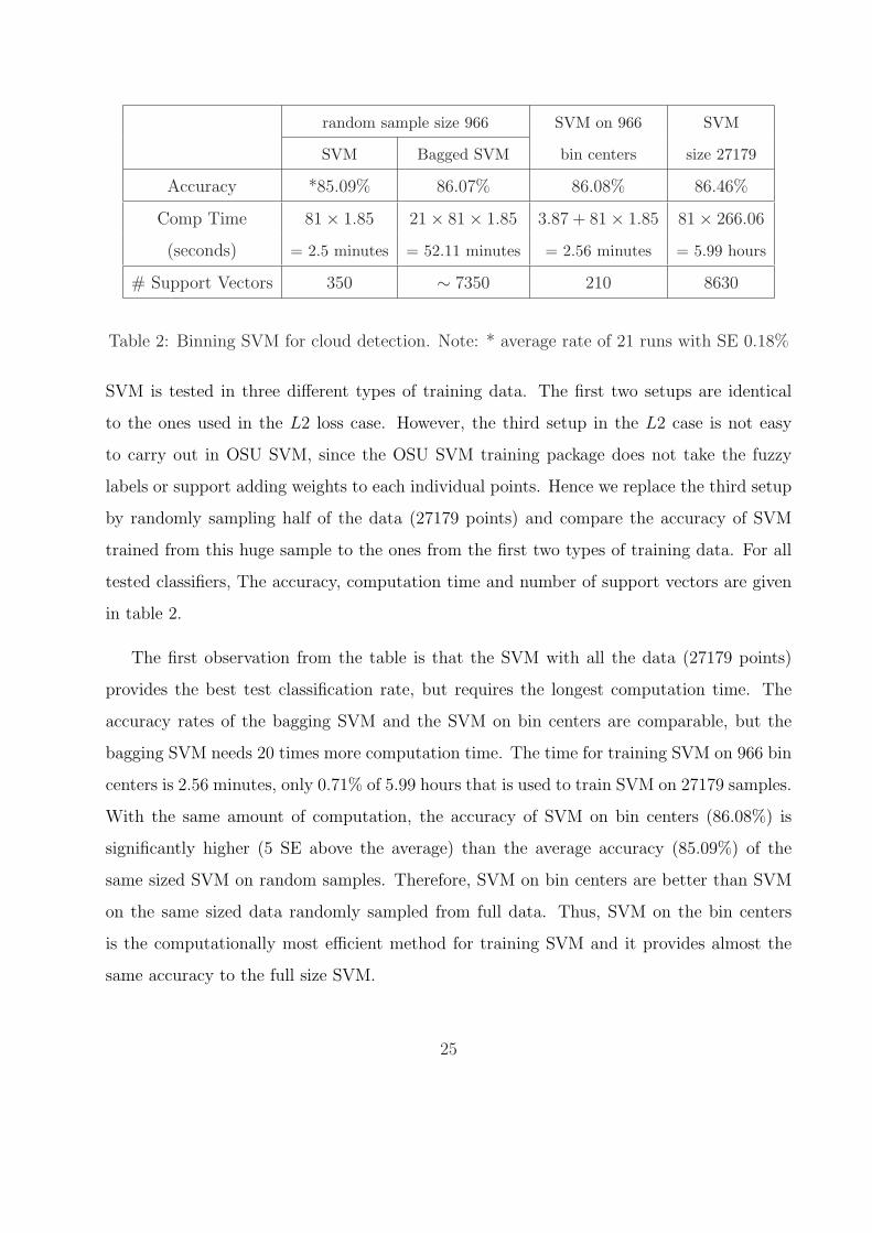
random sample size 966 SVM on 966 SVM
SVM Bagged SVM bin centers size 27179
Accuracy *85.09% 86.07% 86.08% 86.46%
Comp Time 81× 1.85 21× 81× 1.85 3.87 + 81× 1.85 81× 266.06
(seconds) = 2.5 minutes = 52.11 minutes = 2.56 minutes = 5.99 hours
# Support Vectors 350 ∼ 7350 210 8630
Table 2: Binning SVM for cloud detection. Note: * average rate of 21 runs with SE 0.18%
SVM is tested in three different types of training data. The first two setups are identical
to the ones used in the L2 loss case. However, the third setup in the L2 case is not easy
to carry out in OSU SVM, since the OSU SVM training package does not take the fuzzy
labels or support adding weights to each individual points. Hence we replace the third setup
by randomly sampling half of the data (27179 points) and compare the accuracy of SVM
trained from this huge sample to the ones from the first two types of training data. For all
tested classifiers, The accuracy, computation time and number of support vectors are given
in table 2.
The first observation from the table is that the SVM with all the data (27179 points)
provides the best test classification rate, but requires the longest computation time. The
accuracy rates of the bagging SVM and the SVM on bin centers are comparable, but the
bagging SVM needs 20 times more computation time. The time for training SVM on 966 bin
centers is 2.56 minutes, only 0.71% of 5.99 hours that is used to train SVM on 27179 samples.
With the same amount of computation, the accuracy of SVM on bin centers (86.08%) is
significantly higher (5 SE above the average) than the average accuracy (85.09%) of the
same sized SVM on random samples. Therefore, SVM on bin centers are better than SVM
on the same sized data randomly sampled from full data. Thus, SVM on the bin centers
is the computationally most efficient method for training SVM and it provides almost the
same accuracy to the full size SVM.
25

Besides the training time, the number of support vectors determines the computation
time need to classify new data. As shown in the table, SVM on bin centers has the fewest
number of support vectors, so it is the fastest to classify a new point. From the comparison,
it is clear that SVM on the binning data provides almost the best accuracy, fast training,
and fast prediction.
At last, we compare binning with another possible sample-size reduction scheme, clus-
tering. Feng and Mangasarian (2001) has proposed to use the k-mean clustering algorithm
to pick a small proportion of training data for SVM. This method first cluster the data into
m clusters. Although this method reduces the size of training data as well, the computation
of k-means clustering itself is very expensive comparing to that of training SVM, or even
not feasible due to the memory usage when data size is too large. In the cloud detection
problem, clustering 27179 training data into 512 groups takes 21.65 minutes, and the time
increases dramatically when the number of centroid increases. The increase in the require-
ment of computer memory is even worse than the increase in the computation time. The
computer memory runs out when we try to cluster the data into 966 clusters.
Just for comparison, clustering-SVM and binning-SVM on 512 groups provides very close
classification rates, 85.72% and 85.64% respectively, but binning is much faster than cluster-
ing. Running in Matlab, the clustering itself takes 21.65 minutes, which is 376 times of the
computation time (3.45 seconds) of binning data to 512 bins. The number of support vectors
of clustering-SVM and binning-SVM are very close, 145 and 143 respectively, so their testing
times are about the same. Thus binning is more preferred in reducing the computation for
SVM than clustering.
6 Summaries
To reduce the computational burden of the Gaussian kernel regularization methods, we pro-
pose binning on training data. The binning effect on the periodic Gaussian kernel regular-
26

ization method is studied in the nonparametric regression. While reducing the computation
complexity from O(n3) to the order of O(n) or less, the binned estimator keeps the asymp-
totic minimax rates of the periodic Gaussian regularization in the Sobolev spaces.
Simulations in the finite sample regression case suggests that the performance of the
binned periodic Gaussian kernel regularization estimator is comparable to the original es-
timator in terms of the estimation error. In our simulation of binning 120 data points in
20 bins, computing the binned estimator only takes 0.4% of the computation time of the
unbinned estimator, but the binned estimators provide almost the same accuracy. Binning
the Gaussian kernel regularization also gives error rates close to those using the full data in
our simulation.
In the polar cloud detection problem, we tested the binning method on the L2 loss Gaus-
sian kernel regularization and the Gaussian kernel SVM. With the same computation time,
the L2-loss Gaussian kernel regularization on 966 bins achieves better accuracy (79.22%)
than that (71.40%) on 966 randomly sampled data. For SVM, binning reduces the com-
putation time (from 5.99 hours to 2.56 minutes in our example), keeps the classification
accuracy, and speeds up the testing step by providing simpler classifiers with fewer support
vectors (from 8630 to 210). The SVM trained on 966 randomly selected samples has a similar
training time as and a slightly worse test classification rate than the SVM on 966 bins, but
has 67% more support vectors so takes 67% longer to predict on a new data point. The
SVM trained on 512 cluster centers from the k-mean algorithm reports almost the same test
classification rate and a similar number of support vectors as the SVM on 512 bins, but the
k-mean clustering itself takes 375 times more computation time than binning.
In summary, binning can be used as an effective method for dealing with large number
of training data in Gaussian kernel regularization methods. Binning is also more preferred
in reducing the computation for SVM than clustering.
27

Acknowledgements
Tao Shi is partially supported by NSF grant CCR-0106656. Bin Yu is partially supported by
NSF grant CCR-0106656, NSF grant DMS-0306508, ARO grant DAAD 19-01-01-0643, and
the Miller Institute as a Miller Research Professor in Spring 2004. MISR data were obtained
at the courtesy of the NASA Langley Research Center Atmospheric Sciences Data Center.
We’d like to thank Prof. Eugene Clothiaux for providing hand labels of MISR data and Mr.
David Purdy for helpful comments on the presentation of the paper.
28

Appendix
Proof of Theorem 1:
As shown in section 3, the expansion of kernel K(., .) in equation (6) leads to
G(n)i,j = K(xi, xj) = 2
∞∑
l=0
e−l2ω2/2[sin(2πlxi) sin(2πlxj) + cos(2πlxi) cos(2πlxj)] (19)
with xi = in− 1
2n.
In case n is an odd number (n = 2q + 1), any non-negative integer l can be written as
l = kn− h or l = kn + h, where both k and h are integers satisfying k ≥ 0 and 0 ≤ h ≤ q.
For any k ≥ 1, h > 0, and all i,
sin(2π(kn + h)xi) = sin(2πknxi + 2πhxi)
= sin(2πknxi) cos(2πhxi) + cos(2πknxi) sin(2πhxi)
= sin(2kiπ − kπ) cos(2πhxi) + cos(2kiπ − kπ) sin(2πhxi)
= (−1)k sin(2πhxi)
In the same way, we get sin(2π(kn − h)xi) = (−1)k+1 sin(2πhxi), and cos(2π(kn + h)xi) =
cos(2π(kn − h)xi) = (−1)k cos(2πhxi). In case h = 0, we have sin(2πknxi) = 0 and
cos(2πknxi) = (−1)k for all i. Therefore, the Gram matrix G(n) can be written as:
G(n)i,j = dC
0 +
q∑
h=1
[dSh sin(2πhxi) sin(2πhxj) + dC
h cos(2πhxi) cos(2πhxj)] (20)
where
dC0 = 2
∞∑
k=0
(−1)ke−(kn)2ω2/2,
dSh = 2{e−h2ω2/2 +
∞∑
k=1
(−1)k(e−(kn+h)2ω2/2 − e−(kn−h)2ω2/2)},
dCh = 2{e−h2ω2/2 +
∞∑
k=1
(−1)k(e−(kn+h)2ω2/2 + e−(kn−h)2ω2/2)}.
29

Let V(n)0 =
√1n(1, · · · , 1)T , V
(n)2h−1 =
√2n(sin(2πhx1), · · · , sin(2πhxn))T , and
V(n)2h =
√2n(cos(2πhx1), · · · , cos(2πhxn))T , for h = 1, · · · , q. Using the following orthogonal
relationshipsn∑
i=1
sin(2πµxi) sin(2πνxi) = n/2 µ = ν = 1, · · · , q
= 0 µ 6= ν; µ, ν = 0, · · · , qn∑
i=1
cos(2πµxi) cos(2πνxi) = n/2 µ = ν = 1, · · · , q
= 0 µ 6= ν; µ, ν = 0, · · · , qn∑
i=1
cos(2πµxi) = 0 µ = 1, · · · , qn∑
i=1
sin(2πµxi) = 0 µ = 1, · · · , q
we can easily see that V0, · · · , V2q are orthonormal vectors. Furthermore, they are the eigen-
vectors of G(n) with corresponding eigen-values d(n)0 = ndC
0 , d(n)2h−1 = ndS
h/2, and d(n)2h = ndC
h /2,
since G(n) =∑2q
l=0 d(n)l V
(n)l V
(n)Tl . It completes the proof for odd number n = 2q + 1.
For even number n = 2q observations , the eigen-vectors of G(n) are V(n)0 , · · · , V (n)
2q−1 and
eigen-values are d(n)0 , · · · , d(n)
2q−1, while both are the same as defined in the odd number case.
All the proofs for odd numbers n hold here except sin(2πkqxi) = sin(2πkq(i/n− 2/n)) = 0
for all k > 0, which leaves V0, · · · , V2q−2, V2q as the 2q eigen-vectors. The eigen-vectors are
slightly different of those for odd number n, but this difference does not affect the asymptotic
results at all. Therefore, we will use the eigen-structure for odd number observations in the
rest of the paper.
To simple the notation, we can write them eigen-values dl in terms of ρl:
d(n)0 = 2n
∞∑
k=0
(−1)kρ2kn
d(n)l = n{ρl +
∞∑
k=1
(−1)k[ρkn+h + (−1)l−2hρkn−h]}
where l = 1, · · · , n− 1, and h = d(l + 1)/2e, while dae stands for the integer part of a. ¤
30

Proof of Proposition 1:
For x ∈ (0, 1], x as defined in proposition 1, and k ≥ 0
m∑j=1
K(x, xj)cos(2πkxj)
=m∑
j=1
{2∞∑
l=0
exp(−l2ω2/2)cos(2πl(x− xj))cos(2πkxj)}
= 2∞∑
l=0
exp(−l2ω2/2){m∑
j=1
cos(2πl(x− xj))cos(2πkxj)}
=∞∑
l=0
exp(−l2ω2/2){m∑
j=1
cos(2π(lx + (k − l)xj)) + cos(2π(lx− (k + l)xj))}
For any integer r,
m∑j=1
cos(2π(lx + rxj)) =m∑
j=1
cos(2πlx− r
mπ + 2π
r
mj)
= { 0 when rm
is not an integer;
m(−1)r/mcos(2πlx) when rm
is an integer.
Therefore,m∑
j=1
K(x, xj)cos(2πkxj) = d(m)k cos(2πkx)
while d(m)k follows the definition in Proposition ??. It is also true that
∑mj=1 K(x, xj)sin(2πkxj) =
d(m)k sin(2πkx). As shown in Proposition ??, the eigen-vector V
(m)k of G(m) is
√2/mcos(2πxj)
or√
2/msin(2πxj). Therefore,
G(n,m)V(m)k = d
(m)k
√n
mV
(n)k
for all k = 0, 1, · · · ,m. ¤
Proof of Theorem 2:
Following the relationship shown in proposition 1 G(n,m)V (m) =√
nm
V (n,m)diag(d(m)l ), with
V (n,m) as the n by m matrix formed by the first m eigen-vectors of G(m). The projection
matrix SB = G(n,m)V (m)diag( 1
d(m)l +λB
)V (m)T B(m,n) =√
nm
V (n,m)diag(d(m)l
d(m)l +λB
)V (m)T B(m,n).
31

Since B(m,n)B(m,n)T = diag(m/n), the asymptotic variance of the estimator is:
1
n
∑var(yi) =
1
ntrace(ST
BSB)
=1
ntrace(
n
mV (n,m)diag(
d(m)l
d(m)l + λB
)V (m)T B(m,n)B(m,n)T V (m)diag(dm
l
d(m)l + λB
)V (n,m)T )
=1
ntrace(diag(
d(m)l
d(m)l + λB
)2) =1
n
m−1∑
l=0
(d
(m)l
d(m)l + λB
)2
As proved before, limm→∞d(m)l /m = ρl for l > 0 and ρl = 1/βl, we get
1
n
∑var(yi) ∼ 1
n
∑(
ρl
ρl + (λB/m))2 =
1
n
∑(1 +
βlλB
m)−2
Proof of Theorem 3:
The bias of the binned estimator is 1n
∑Bias2(yi) = 1
n((SB − I)F )T ((SB − I)F ). Let C(n,m)
denote a n by m matrix of (Im×m : 0m×(n−m))T . The term (SB − I)F is expanded as:
(SB − I)F = (G(n,m)(G(m) + λBI)−1B(m,n) − I)V (n)Θ(n)
=
√n
mV (n,m)diag(
d(m)l
d(m)l + λB
)V (m)T B(m,n)V (n)Θ(n) − V (n)Θ(n)
= V (n)C(n,m)diag(
√n
m
d(m)l
d(m)l + λB
)V (m)T B(m,n)V (n)Θ(n) − V (n)Θ(n)
= V (n)(C(n,m)diag(
√n
m
d(m)l
d(m)l + λB
)V (m)T B(m,n)V (n) − I(n))Θ(n)
, V (n)A(n,n)Θ(n)
Now, let us study V (m)T B(m,n)V (n). We first start with one of the V (n)’s eigen-vectors:√
2/n(cos2πkx1, · · · , cos2πkxn)T .
B(m,n)(cos2πkx1, · · · , cos2πkxn)T
= ((cos2πkx1 + · · ·+ cos2πkxp)/p, · · · , (cos2πkxn−p+1 + · · ·+ cos2πkxn)/p)T
= w(m,n)k (cos2πkx1, · · · , cos2πkxm)T ,
while w(m,n)k is a constant as function of n, m, and k. When p = n/m is an odd num-
ber, (xrp+1, · · · , xrp+p) is expressed as (xr − (p − 1)/2n, · · · , xr, · · · , xr + (p − 1)/2n). Thus,
32

cos2πkxrp+1 + · · ·+ cos2πkxrp+p = [1 + 2cos2πkn
+ · · ·+ 2cos2πk((p−1)/2)n
]cos2πkxr. Therefore,
w(m,n)k = (1 +
∑(p−1)/2j=1 2cos2πkj
n)/p for odd number p. It is straightforward to show that
w(m,n)k = (
∑p/2j=1 2cos2πkj−πk
n)/p for even number p. In the same way, we have
B(m,n)(sin2πkx1, · · · , sin2πkxn)T = w(m,n)k (sin2πkx1, · · · , sin2πkxm)T
Let j0 = d(j + 1)/2e for 0 ≤ j ≤ n − 1. Following the proof of proposition 1 and assuming
m = 2q + 1 as an odd number, we can write any j0 as j0 = hm − i0 or j0 = hm + i0 with
0 ≤ i0 ≤ q, where i0 is a function of j and m. For the situation of odd number j and
j0 = hm + i0, we have
B(m,n)V(n)j = B(m,n)
√2/n(sin2πj0x1, · · · , sin2πj0xn)T
= w(m,n)
j0
√2/n(sin2πj0x1, · · · , sin2πj0xn)T
= w(m,n)
j0
√2/n(−1)h(sin2πi0x1, · · · , sin2πi0xn)T
= w(m,n)
j0
√m/n(−1)hV
(m)
2i0−1.
Similarly, we can derived the equation for even number j and j0 = hm− i0. So the structure
of V(m)i
TB(m,n)V
(n)j is:
V(m)i
TB(m,n)V
(n)j =
√m/n w
(m,n)
j0 cm,ni,j V
(m)i
TV
(m)
2i0+((−1)j−1)/2
where the constant cm,ni,j equals (−1)h when (1) j is even or (2) j is odd and j0 = hm +
i0, and it equals (−1)h+1 otherwise. Therefore, the matrix is nonzero only when i =
2i0 + ((−1)j − 1)/2 , j. Let us denote µij = w(m,n)j0
cm,ni,j for the nonzero elements of matrix
V (m)T B(m,n)V (n), which is in the following shape:
√m
n
µ0,0 0 · · · 0 0 0 · · · µ0,2m−1 0 0 · · ·0 µ1,1 0 0 0 0 · · · 0 µ1,2m 0 · · ·0 0 · · · 0 µm−2,m 0 · · · 0 0 · · · · · ·0 0 · · · µm−1,m−1 0 µm−1,m+1 0 · · · 0 0 · · ·
m×n
Since A(n,n) = C(n,m)diag(√
nm
d(m)l
d(m)l +λB
)V (m)T B(m,n)V (n) − I(n), the entry of of A(n,n) is aij =
33

d(m)i
d(m)i +λB
µij − I(j = i) for 0 ≤ i < m, and aij = −I(j = i) for all i ≥ m. So A(n,n) is
diag(
d(m)l µll
d(m)l +λB
)− I(m,m) A(m,n−m)
0 −I(n−m,n−m)
n×n
Now let us study of the bias as a whole term.
1
n
∑Bias2(yi) =
1
n((SB − I)F )T ((SB − I)F )
=1
n(V (n)A(n,n)Θ(n))T V (n)A(n,n)Θ(n)
=1
n(Θ(n)
√n
)T A(n,n)T A(n,n) Θ(n)
√n
=m−1∑j=0
(Θ
(n)j√n
)2(d
(m)j µjj
d(m)j + λB
− 1)2 +n−1∑j=m
(Θ
(n)j√n
)2(1 + (d
(m)
jµjj
d(m)
j+ λB
)2)
+m−1∑
k=0
n−1∑j=m
Θ(n)k Θ
(n)j
n(
d(m)k µkk
d(m)k + λB
− 1)(d
(m)k µkj
d(m)k + λB
)I(k = j)
+n−1∑
k=m
m−1∑j=0
Θ(n)k Θ
(n)j
n(
d(m)k µkj
d(m)k + λB
)(d
(m)j µjj
d(m)j + λB
− 1)I(j = k)
+n−1∑
k=m
n−1∑j=m
Θ(n)k Θ
(n)j
n(
d(m)k µkj
d(m)k + λB
)(d
(m)k µkj
d(m)k + λB
)I(j = k)I(j 6= k)
∼m−1∑j=0
(Θ
(n)j√n
)2(d
(m)j µjj
d(m)j + λB
− 1)2 +n−1∑j=m
(Θ
(n)j√n
)2(1 + (d
(m)
jµjj
d(m)
j+ λB
)2)
when n →∞, m →∞ and dm/(dm+λ) → 0. Since cm,nj,j = 1 for j = 1, · · · ,m and w
(m,n)j → 1
as m/n → 0, we have µjj → 1. Therefore,
1
n
∑Bias2(yi) ∼
m−1∑j=0
θ2j (
ρj
ρj + λB/m− 1)2 +
∞∑j=m
θj2
=m−1∑j=0
θ2j (
λB/m
ρj + λB/m)2 +
∞∑j=m
θj2
=m−1∑j=0
θ2j (
βjλB/m
1 + βjλB/m)2 +
∞∑j=m
θj2
¤
34

References
[1] Breiman, L. (1996a). Bagging Predictors. Machine Learning, 24 No. 2 123-140.
[2] Brown, L.D. and Low, M.G. (1996). Asymptotic Equivalence of Nonparametric Regres-
sion and White Noise. Annals of Statistics 24 2384-2398.
[3] Buhlmann, P. and Yu, B. (2002). Analyzing Bagging. Annals of Statistics 30 927-961.
[4] Evgeniou, T., Pontil, M., and Poggio, T. (2000). Regularization Networks and Support
Vector Machines. Advances in Computational Mathematics 13 1-50.
[5] Feng, G. and Mangasarian, O. L. (2001) Semi-Supervised Support Vector Machines for
Unlabeled Data Classification. Optimization Methods and Software. Kluwer Academic
Publishers, Boston.
[6] Girosi Girosi, F., Jones, M. and Poggio, T. (1993). Priors, Stabilizers and Basis Func-
tions: from regularization to radial, tensor and additive splines. M.I.T. Artificial Intel-
ligence Laboratory Memo 1430, C.B.C.I. Paper 75.
[7] Hall, P., Park, B. U., and Turlach, B.A. (1998) A note on design transformation and
binning in nonparametric curve estimation. Biometrika, 85(2) 469-476.
[8] Johnstone, I. M. (1998). Function Estimation in Gaussian Noise: Sequence Models.
Draft of a monograph. http://www-stat.stanford.edu/
[9] Lin, Y. and Brown, L. D. (2004). Statistical Properties of the Method of Regularization
with Periodic Gaussian Reproducing Kernel. Annals of Statistics. 32 1723-1743.
[10] Mallows, C.L. (1973). Some comments on Cp. Technometrics 15 661-675.
[11] Shi, T., Yu, B., Clothiaux, E.E., Braverman, A. (2004) Cloud Detection over Snow and
Ice based on MISR Data. Technical Report 663, Department of Statistics, University of
California.
35

[12] Smola, A.J., Schoolkopf, B., and Muller, K. (1998). The connection between regulariza-
tion operators and support vector kernels. Neural Networks 11 637-649.
[13] Vapnik, V.(1995). The Nature of Statistical Learning Theory. Springer, N.Y., 1995.
[14] Wahba, G. (1990). Spline Models for Obersvational Data. Society for Industrial and
Applied Mathematics. Philadelphia, Pennsylvania.
[15] Wahba, G., Lin, Y., and Zhang, H. (1999). GACV for Support Vector Machines, or
Another Way to Look at Margin-Like Quantities, Advanced in Large Margin Classifiers.
[16] Williamson, R. C., Smola, A. J. and Scholkopf, B. (2001). Generalization performance
of regularization networks and support vector machines via entropy numbers of compact
operators. IEEE Transactions on Information Theory 47, 2516-2532.
[17] Williams, C., and Seeger, M. (2000). The Effect of the Input Density Distribution on
Kernel-based Classifiers. International Conference on Machine Learning 17, 1159-1166.
36