22 TRANSPORTATION RESEARCH RECORD 1303

Lateral Clearance to Vision Obstacles on Horizontal Curves

SAID M. EASA

Eva luation of the sight distance adequacy on highway horizontal curve with single or multiple ob ·racles requires determi nation of the miJ1imum sight distanc on the curve. he currem method of e tabli hing such a minimum is to plot the sight distance profile for the given curve and ob tacle. Approximate relationships have been d veloped f r e tablishing the ight distance profile . .How­ever. there i. no explicit , exact olution available for determining the minimum . ight di. ranee on rhe curve. - xact formulas have been derived to relate the available ight distance to the L:in:uh1r curve parameters, lateral clearance of the ob tacle. it location along rhe cur c. and rhe lo ation of observer and objecl. These relationship arc then used to derive closed-form olution of the minimum ight dist11nce , ,,.. To facilitate practical u e, values of S., are estalilished for typical ranges of the curve parameter , lateral clearance, and ob tacle location. Values of the maximum lateral clearance, wbich is required in de ign, are al o provided. The methodology and results should be valuable in the opera­tional and cost-effectiveness analysi of highway locations with restricted sight distances.

The sight distance on highway horizontal curves may be re­stricted by such physical features as longitudinal barriers, cut slopes, foliage, and other structures. For safe operations, the available sight distance at any point on the traveled way must be greater than the sight distance needed for stopping, pass­ing, or decision at complex locations . The available sight distance is a function of the horizontal curve parameters, locations of the observer and object, and the location of the vision-limiting obstacle inside the curve.

The stopping sight distance (SSD), presented by AASHTO (J - 4), is one of the basic considerations in the design of highways. Design values for SSD applicable to all highways are presented by AASHTO. A new approach to SSD that considers the functional classifications of highways was re­cently presented by Neuman (5). Design values for passing sight distance (PSD) involving passenger cars on two-lane highways are presented in AASHTO's 1984 Policy on Geo­metric Design of Highways and Streets (Green Book) (4). Design values for PSD for all combinations of passing in­volving a passenger car and a truck have been developed by Harwood and Glennon (6) . These design values are based on a model developed by Glennon (7) that logically accounts for the kinematic relationships among the passing, passed , and opposing vehicles and explicitly contains vehicle-length var­iables . Design values for decision sight distance (DSD) are presented by AASHTO (4) and Neuman (5), and their use­fulness and application have been evaluated by McGee (8) .

A number of models exist that relate the available sight distance and the lateral clearance on horizontal curves.

Department of Civil Engineering, Lakehead University, Thunder Bay, Ontario, Canada P7B SEl.

AASHTO presents a model that relates the sight distance, S,,,, and maximum lateral clearance, M, for S,,, :s= L, where L is the length of the curve ( 4) . The case S,,, > L is not presented by AASHTO. When either the vehicle or vision obstacle is situated near the ends of the curve, the less clear­ance is needed. The studies by Olson et al. (9) , Neuman and Glennon (10), and Glennon (11) show that when the vehicle is on Lht: La11gent within a distance S from the point of cur­vature, PC, the maximum lateral clearance needed varies from 0 to M (when the vehicle is at PC). The required lateral clearance for all points within S/2 beyond PC is also less than M. For these situations, AASHTO recommends the use of a graphical procedure or the curves empirically developed by Raymond (12).

To eliminate the need for the graphical procedure , Waissi and Cleveland (13), on the basis of the results of the NCHRP report by Olson et al. (9), derived approximate relationships that relate the available sight distance to the horizontal curve parameters, locations of observer and road object, location of obstacle, and lateral clearance to a single obstacle to vision located inside the curve. Relationships for determining the maximum lateral clearance for S,,, > L are also presented.

For a given obstacle on the curve, the available sight dis­tance varies as the observer moves along the tangent and curve . Clearly, there is a minimum value of sight distance on Lht: Lraveled path that determines the adequacy of sight dis­tance on the curve. There is no explicit, exact solution avail­able for determining this minimum sight distance. The pur­pose of this paper is threefold:

1. To derive exact relationships for determining the avail­able sight distance for arbitrary locations of the observer and obstacle,

2. On the basis of the preceding, to develop relationships for determining the minimum sight distance, and

3. To establish evaluation and design values for practical use.

THEORETICAL DEVELOPMENT

Relationships for determining the minimum sight distance, S,,,, are developed for a single obstacle located on the inside of a simple horizontal curve between PC and PT (point of tangency) . Both the observer and object are assumed to be located on the centerline of the inside lane. Three cases are considered:

•Case 1: Observer before PC and object beyond PT,

Easa

• Case 2: Observer before PC and object on curve, and • Case 3: Observer and object on curve.

Case 1: Observer Before PC and Object Beyond PT

The geometry of this case is shown in Figure 1. As the observer moves toward PC, the available sight distance decreases, reaches a minimum value, and then increases again. The lateral clear­ance requirements should be based on this minimum value. In Figure 1, x 1 is the distance from the observer to PC, and x 2 is the distance from the object to PT.

Available Sight Distance

The available sight distance is given by

(1)

where S equals available sight distance, and L equals curve length.

With the law of sines for triangles abPT and acPC, x 1 and x 2 can be expressed in terms of the angles 01 and 02 , shown in Figure 1, as

x 1 = m 1 sin0/sin(01 + ex)

x2 = m2 sin82/sin(82 + r3)

where

m 1 = distance from the obstacle to PC, m 2 = distance from the obstacle to PT,

(2)

(3)

ex = angle at PC between the tangent and the line to the obstacle, and

r3 = angle at PT between the tangent and the line to the obstacle.

Note that in Equation 2, sin(0 1 + ex) = sin(180 - 81 -

ex), and similarly for Equation 3. These four elements, which are constant for a given curve and obstacle, are computed using triangles oaPC and oaPT as follows:

m 1 = [R2 + (R - m)2 - 2R(R - m) cos/1]

112 (4)

m2 = [R2 + (R - m)2 - 2R(R - m) cos(/ - / 1)]

112 (5)

4 Designate s obstacle

FIGURE 1 Case 1: Observer before PC and object beyond PT.

23

ex = 90° + cos - 1{[-(R - m)2 + R2 + mT]/2Rm 1} (6)

r3 = 90° + cos- 1{[ - (R - m) 2 + R2 + m~]/2Rm2} (7)

where

R = curve radius, m = lateral clearance between the centerline of the inside

lane and obstacle, 11 = central angle from PC to the obstacle, and I = central angle from PC to PT.

The angles 01 and 02 are related by

(8)

Since L aPCo = ex - 90° and L aPTo = r3 - 90°, the angle J is obtained as follows:

J = ex + r3 + I - 180° (9)

Substituting 02 of Equation 8 into Equation 3, the available sight distance of Equation 1 can be written as

S = L + [m 1 sin6/sin(0 1 + ex)]

+ [m2 sin(8 1 + J)/sin(0 1 + J - r3)] (10)

in which the curve length L equals RTI//180.

Condition for S,,,

Differentiating Equation 10 with respect to 01 and equating dS/d0 1 to zero gives

sin(o; + ex)/sin(0; + J - r3) = (m 1 sinex/m2 sinr3) 112 (11)

in which Oi is the critical angle corresponding to the minimum sight distance, S,,,. The derivation of Equation 11 is included in Appendix A. A successive approximation method for solv­ing Equation 11 to determine Oi is given in Appendix B. Note that Equation 11 implies that Oi must be greater than (r3 - J). For equal or smaller values, the line of sight from the observer to the obstacle does not intersect with the tangent beyond PT. After determining Oi, S,,, is computed by sub­stituting e7 into Equation 10.

If the obstacle lies at the midpoint of the curve(///= 0.5), then m 1 = m2 and ex = r3. With these values, Equation 11 yields Oi + ex = 180 - (Si + J - r3) (note that ex 1= J -r3 is based on Equation 9). Thus,

e; = (180° - J)/2 for I/I = 0.5 (12)

which implies that x 1 = x2 , as expected .

Case 2: Observer Before PC and Object on Curve

In this case, the observer is on the tangent at a distance x 1

from PC, and the object is on the curve at a distance l 1 from PC (Figure 2).

24 TRANSPORTATION RESEARCH RECORD 1303

FIGURE 2 Case 2: Observer before PC and object on curve (l,II ,;; 0.5).

Available Sight Distance

The available sight distance is given by

(13)

where L 1 , the distance from PC to the object, is given by

(14)

and x 1 is given by Equation 2 (m 1 and O'. are given by Equations 4 and 6). / 2 is the central angle between PC and the object (in radians) . The angle oda = 01 + O'. - 90°. Therefore, using triangle obd, 12 is obtained:

(15)

Using triangles oab and oad, respectively, 'Y and Q> are obtained:

'Y = sin - 1[(R - m) sinQ>/R]

Now Equation 13 can be written as follows:

S = R/2 + (m 1 sin0/sin(01 + O'.)]

Condition for S,,,

(16)

(17)

(18)

Differentiating Equation 18 with respect to 01 and equating dS/d0 1 to zero give (Appendix A)

R sin2(0; + O'.)

(R - m) sin(0; + O'. + /1) 1 (19)

(R2 - (R - m)2 cos2(0; + O'. + / 1)]112

Solving Equation 19 by successive approximations gives the critical angle 0i (Appendix B). S,,, is then computed by sub­stituting 0i into Equation 18.

Because of the symmetry of the horizontal curve, Case 2 may occur only when I/I is less than 0.5. For I/I greater than 0.5, the minimum sight distance occurs when the observer is on the curve and the object is beyond PT. The solution of this situation is also given by Equations 13- 19 after switching the positions of PC and PT, and of the observer and object.

• Case 3: Observer and Object on Curve

In Case 3, both observer and object are on the curve. Figure 3 shows the geometry of this case. Let / 3 denote the central angle from the observer to the obstacle and / 4 the central angle from the obstacle to the perpendicular line od. Using triangle ace, tan/4 = aelec. But ae = (R - m) - oe. From triangle oec, ec = R sin/3 and oe = R cos/3 . Thus,

(20)

where / 3 , which equals / 1 - L coPC, is given by

/ 3 = / 1 - (180x/ rrR) (21)

and x 1 is the distance along the curve between the observer and PC

Available Sight Distance

The available sight distance is given by (Figure 3)

(22)

where / 3 and / 4 are in radians. Substituting for / 4 from Equa­tion 20 into Equation 22 gives

Condition for S,,,

Differentiating Equation 23 with respect to / 3 and equating dSld/3 to zero gives (Appendix A)

FIGURE 3 Case 3: Observer and object on curve.

[R(l - cos!;) - m](R - m) = 0 (24)

from which

m = R(l - cos!;) (25)

Substituting for m into Equation 20 gives /4 0, which implie that S,,. occur when the observer and object are at equal di tanc from the ob tacle. Thu · from Equation 22, S.,, = nRf!/90 or t; = 90S,,/r.R (where /'i is in degrees).

ubsti tuting for I; int Equation 25 gives

m = R[l - cos(90SmlnR)] (26)

which is the formula pre ented by AASHTO (4). It is clear that for Case 3, Sm is independent of the location of the obstacle for any given value of m.

Conditions for Case Determination

The geometry of the conditions for different cases is shown in Figure 4. Line oc is a radial line passing through the ob­stacle. The line from PC to d is perpendicular to this radial line. If m is less than cb, this is Case 3. If m is greater than cb but less than ca, this is Case 2. If m is equal to or greater than ca, this may be Case 1 or 2.

Given R, I, m, and / 1 , the following steps are used to determine the respective case and the minimum sight distance:

FIGURE 4 Geometry of the conditions for case determination.

1. S,,, corresponds to Case 3 if the following condition is satisfied:

m s R[l - cos/'] /' = min{/1 , I - / 1} (27)

The right-hand side equals cb in Figure 4. If this condition is not satisfied, go to the next step.

2. S.,, corresponds to Case 2 if the following condition is satisfied:

m < R{l - [cos(//2)/cos(//2 - / 1]} (28)

The right-hand side of Equation 28 equal ca in Figure 4. Thi is the rarual di lance from the curve center to the line of sight when the ob erver i at P and object is at PT. if this condition is not satisfied, Sm may correspond to Case 1 or 2. Go to the next step.

3. To determine whether S,,, corresponds to Cas 1 or 2, first calculate er, X1, and X2 for Case 1. If Xi and X 2 are positive or zero, then Sm corresponds to Case 1. Otherwise, Sm cor­responds to Case 2.

The following numerical example illustrates these teps. upp se that R = 1,500 ft , I = 3 .2°, m = 0 ft and /1 =

7.64°. ln Step 1, the right-hand side of Equation 27 equals 13.32 ft and Equation 27 i · not atisfied. Ther fore , l11is is not Case 3. In Step 2, the right-hand side of Equation 28 equals 53. 74 ft. Therefore, Equation 28 is satisfied and S'" corre ponds to Ca e 2. For Case 2, calculate m 1 = 200.12 fl (Equati.on 4) and~ = 167.58° (Equation 6). olving Equation 19 by ucce ive approximat ion (Appendix B) gives OT =

3.25°. Then , <f> = 88.47° (Equation 17) , 'Y = 78.42° (Equation 16) , /2 = 20.75° (Equation 15), and S,,, = 614 ft (Equa­tion 18) .

PRACTICAL ASPECTS

The minimum sight distance on a horizontal curve must be determined to know whether the required sight di tance ( top­ping decision, or pa ing) is satisfied. The sight distance pro­file is a nece · ary input to the co ·t-effectivene s ana ly is of locations with restricted ight distance . ln thi ection the

26

sight distance profile, the application of the presented meth­odology to multiple obstacles, and a comparison with the NCHRP method are discussed.

Sight Distance Profile

The sight distance profile for a given obstacle for different values of the lateral clearance is shown in Figure 5. The ob­stacle is located at 1/1 = 0.3. The horizontal axis shows the location of the observer at various points of the tangent and curve. The PC is designated as the reference point, with the locations before it being negative and the locations beyond it being positive. The vertical axis shows the available sight distance for any given location of the observer. For example, for m = 15 ft, the minimum sight distance ( 435 ft) occurs when the observer is about 90 ft beyond PC. The sight distance profile is established using the developed relationships by computing the available sight distance for successive values of x 1 • Unlike vertical curves, the minimum sight distance on a horizontal curve with a single obstacle occurs at a specific point on the traveled way rather than through a section of the traveled way.

For locations with restricted sight distances, the sight dis­tance profile provides the length of the road within which the sight distance is restricted. This length is required for the operational and cost-effectiveness analysis developed by Neu­man et al. (14). The probability that a critical event will occur

§: Cl)

ui (.) z < I-Cl)

Ci I-I (!)

iii w --' aJ < --' ;;: > <

1500

1000

500

Parameters =

R=1500ft I= 38.2' 1,11 = 0.3

Required SD • 600 ft

TRANSPORTATION RESEARCH RECORD 1303

at the location is directly proportional to the length of re­stricted sight distance. For example, if the required sight dis­tance in Figure 5 is 600 ft and m = 15 ft, the SD profile shows that the length with a restricted sight distance is about 400 ft.

Application to Multiple Obstacles

For a horizontal curve with multiple obstacles, the sight dis­tance profile of one obstacle interferes with the profiles of other obstacles. The actual sight distance profile is an enve­lop of the individual profiles, as shown in Figure 6. The horizontal curve has four obstacles with the indicalecl lateral clearances and locations on the curve. It is clear that Obstacle 2 is critical because it gives the least value of Sm ( 430 ft). The minimum sight distances can be determined using the devel­oped relationships by considering each obstacl as a inglc obstacle (note that some ob tacles may not have their mini­mum values on the sight distance envelope).

The interface among the profiles of various obstacles is an important element that should be considered in improving the sight distance on the curve. As noted in Figure 6, Sm on the curve can be improved by increasing the lateral clearance at Obstacle 2, but only to Sm = 450, which corresponds to Ob­stacle 4. Any further improvement in sight distance would r quire increasing the lateral clearances at both Ob tacles 2 and 4, and o on. Thus, an obstacle that is currently not critical may becomr. c:ritic11J as other obstacles are displaced.

/ Length with "' I restricted SD

'/ c11 /-Locus of Sm

I o ........... ~ ........... ~_.___...._ ...... ~~1~ ........... ~ ...... ~...__._~ ........... ~~~...__._~ 1000 500 Ob:acle 0 -500 -800

PT PC

LOCATION OF OBSERVER (ft}

FIGURE 5 Sight distance profile on horizontal curve for different lateral clearances.

Easa 27

Parameters :

R = 1500 ft 1500 I =382'

~ (/) ... ui " 0 () lit z Jl <( 0 I- 1000 (/)

Ci I-I Cl (/)

w _J

m <(

Sight Distance _5 _J

4: > Envelope <(

500

m(ft) 10 20 15 30

obstacle no. 4 3 2

Location • • • .... 0 1400 1000 500 0 -400

PT PC

LOCATION OF OBSERVER (ft)

FIGURE 6 Sight distance envelope on horizontal curve with multiple obstacles.

Comparison with NCHRP Method

As previously indicated, the geometric relationships of the NCHRP report give the available sight distance for different locations of observer, object, and obstacle (9,13). Using these relationships, the available sight distance was computed for consecutive locations of the observer, and the sight distance profile was plotted as shown in Figure 7 (R = 1,000 ft, m = 80 ft, and///= 0.1). The sight distance profile based on the relationships presented in this paper is also shown. The S,,, values of the NCHRP and presented methods are 1,020 ft and 950 ft, respectively. Thus, the NCHRP method overes­timates S,,, by about 7 percent. The differences in S,,, were found to be much larger for 1/1 = 0 and smaller radii. How­ever, the differences decrease as I// approaches 0.5. The two methods give almost identical results of S,,, for I// = 0.5 in Case 1 and for any value of I/I in Case 3.

Although the difference between the 111inimw11 ight di -tance of the two methods is not large, the re pectiv sigh t distance pr file · are considernbly different. If th required ight di tance at th l cuLion is 1, lOO ft , for exampl the

lengths of the restricted ight distance provided by the NCH RP and presented methods will be about 250 ft and 400 ft, re­spectively. Such a difference may affect the operational and cost-effectivene s analy i of restricted locations (10,14) .

The difference between the two method is caused by an a sumption in the N HRP relation ·hips. The relati n hips implicitly a ume that the line connecting the ob~erver and object to the curve center form equal angles with a perpen­dicular line drawn from the center to the line of sight. This

assumption is not generally valid for computing the available sight distance. In addition, for computing S,,,, this assumption is exact only for Case 1 (when 1/1 = 0.5) and Case 3.

EVALUATION AND DESIGN VALUES

To facilitate evaluation of the sigh t di ·tance adequacy on . horizontal curves , the developed relati n hip were u ed to establish values of the minimum sight distance for different characteristics of the curve and obstacle. The values are given in Tables 1 and 2, which are applicable to stopping, decision , and passing sight distances. Tables 1 and 2 can be used to

1. Determine the minimum sight distance on an existing curve and obstacles,

2. Determine the required lateral clearances to maintain a required minimum sight distance, and

3. Determine the critical lateral clearance (for design) that maintains a required minimum sight distance.

The critical lateral clearance, M, is the largest value of m for given S,,,, R, and /. For S,,, s L, the critical value is presented by AASHTO (4). For S,,. > L, a formula and a nomograph for determining M were presented by Waissi and Cleveland (13). In Tables 1and2, the critical lateral clearance for S,,, s L or S,,, > Lis the lateral clearance for /Ji = 0.5. Figure 8 illustrates the results for R = 1,500 ft and I = 40°. As noted, there is a great difference between the lateral clear­ance requirements when the obstacle lies at PC (or PT) and

TABLE 1

Cent. Angle (dP.g)

5 5 5 5 5 5

10 10 10 10 10 10

20 20 20 20 20 20

30 30 30 30 30 30

40 40 40 40 40 40

a Later al

'!:. w (.) z <( f-~ 0 f-I i:2 (/)

w _J

CD <( _J

<( > <(

2000

1500

1000

Obj~v~r Obslacle

I I I I I I \ \

_Presented Method

Parameters 1

A= 1000 ft m = 80 It I = 38,2' 1, = 3.82°

NC HAP / Method--.,.....

/ /

/ /

\ / /

Required SD / ---------r -------_,.....

Obstacle .. 500 ,~o-o""""""--""""'o-------~,o~o:-----_~2~0~0 --""""'-_~300~-----~4~00~----,_s~o~o------s~o~o,...----_-7~00

PC LOCATION OF OBSERVER (ft)

FIGURE 7 Comparison between sight distance profiles of presented and NCHRP methods.

MINIMUM SIGHT DISTANCE ON HORIZONTAL CURVE WITH SINGLE OBSTACLE (R

Obst. Curve Radius (ft) Loe. (T 1/I) 200 400 600

m- 20a 40 60 80 100 20 40 60 80 100 20 40 60 80 100

0.0 940 1850 2770 3690 4600 950 1870 2790 3700 4620 970 1890 280 0 3720 4640 0.1 930 1850 2770 3680 4600 950 1870 2780 3700 4610 960 1880 2800 3710 4630 0.2 930 1850 2770 3680 4600 940 1860 2780 3690 4610 960 1870 2790 3710 4620 0.3 930 1850 2760 3680 4600 940 1860 2770 3690 4610 950 1870 2790 3700 4620 0 . 4 930 1850 2760 3680 4600 940 1860 2770 3690 4610 950 1870 2780 3700 4620 0.5 930 1850 276 0 3680 4600 940 1860 2770 3690 4610 950 1860 2780 3700 4620

0.0 500 950 1410 1870 2320 530 990 1440 1900 2360 560 1020 1480 1940 2390 0.1 490 950 1410 1860 2320 520 980 1430 1890 2350 540 1000 1460 1920 2380 0.2 490 940 1400 1860 2320 510 970 1430 1880 2340 530 990 1450 1910 2370 0.3 480 940 1400 1860 2320 500 960 1420 1880 2340 520 980 1440 1900 2360 0.4 480 940 1400 1860 2320 500 960 1420 1880 2330 520 980 1430 1890 2350 0.5 480 940 1400 1860 2320 500 960 1420 1870 2330 520 970 1430 1890 2350

0 . 0 300 530 750 980 1210 360 590 820 1050 1280 410 650 880 1110 1340 0.1 290 520 750 970 1200 340 570 800 1030 1260 390 620 850 1080 1310 0.2 280 510 740 970 1200 320 550 780 1010 1240 360 600 830 1060 1290 0.3 270 500 730 960 1190 310 540 770 1000 1230 350 580 810 1040 1270 0.4 270 500 730 960 1190 310 540 770 1000 1230 340 570 800 1030 1260 0.5 270 500 730 960 1190 300 530 760 1000 1230 340 570 800 1030 1260

0.0 250 400 sso 700 850 330 490 650 800 950 410 580 740 890 1050 0 . 1 230 390 540 690 850 300 470 620 770 930 370 540 700 850 1010 0.2 220 380 530 690 840 290 440 600 750 910 340 510 660 820 970 0.3 220 370 530 680 830 270 430 580 740 890 320 490 640 BOO 950 0.4 210 370 520 680 830 270 420 570 730 880 320 470 630 780 940 0.5 210 370 520 670 830 260 420 570 730 880 310 470 620 780 930

0.0 240 350 470 580 690 330 470 590 700 820 410 570 700 820 940 0.1 220 340 450 570 680 300 430 550 670 790 360 520 650 770 890 0.2 210 320 440 550 670 280 410 530 640 760 330 480 610 730 850 0 . 3 200 310 430 550 660 260 390 510 620 740 320 460 580 700 820 0.4 190 310 430 540 660 260 380 500 610 730 310 450 570 680 800 0.5 190 310 420 540 660 260 380 490 610 730 310 450 560 680 BOO

clearance (ft)

No t e : minimum sight distances are expressed in feet.

200 TO 800 ft)

800

20 40 60 80 100

990 1910 2820 3740 4650 980 1890 2810 3730 4640 970 1880 2800 3720 4630 960 1880 2800 3710 4630 960 1870 2790 3710 4630 960 1870 2790 3710 4620

590 1050 1510 1970 2430 570 1030 1490 1950 2410 5 50 1010 1470 1930 2390 540 1000 1460 1920 2380 540 990 1450 1910 2370 5 30 990 1450 1910 2370

470 710 950 1180 1410 430 670 910 1140 1370 410 640 870 1100 1340 390 620 850 1080 1310 380 610 840 1070 1300 370 600 830 1060 1300

470 660 820 980 1140 420 610 ·110 Y~U 1080 390 570 730 880 1040 370 540 700 850 1010 360 530 680 840 990 360 520 680 830 980

470 660 800 930 1050 400 590 740 860 980 370 550 690 810 930 360 520 660 770 890 360 510 640 750 870 360 510 630 750 870

TABLE 2 MINIMUM SIGHT DISTANCE ON HORIZONTAL CURVE WITH SINGLE OBSTACLE (R 1,000 TO 3,000 ft)

Cent . Obst. Curve Radius (ft) Angle Loe. (deg) (I1/I) 1000 1500 2000 3000

m- 20a 40 60 BO 100 20 40 60 BO 100 20 40 60 BO 100 20 40 60 BO 100

5 0.0 1010 1920 2B40 3760 4670 1050 1970 2B80 3BOO 4710 1090 2010 2920 3B40 4760 1170 2090 3010 3930 4840 5 0.1 990 1910 2820 3740 4660 1030 1940 2B60 3780 4690 1060 19BO 2890 3Bl0 4730 1130 2050 2960 3880 4800 5 0.2 980 1900 2Bl0 3730 4650 1010 1930 2840 3760 4680 1040 1950 2870 3790 4710 1090 2010 2930 3850 4760 5 0.3 970 1890 2810 3720 4640 1000 1910 2B30 3750 4660 1020 1940 2B60 3770 4690 1070 1990 2910 3B20 4740 5 0.4 970 lBBO 2800 3720 4630 990 1910 2B20 3740 4660 1010 1930 2B50 3760 46BO 1060 1970 2B90 3Bl0 4730 5 0.5 960 lBBO 2800 3720 4630 990 1900 2B20 3740 4650 1010 1930 2B40 3760 46BO 1050 1970 2B90 3800 4720

10 0 . 0 620 1090 1550 2000 2460 700 1170 1630 2090 2550 770 1240 1710 2170 2630 910 1390 1B60 2330 2790 10 0.1 600 1060 1520 19BO 2430 660 1130 1590 2050 2500 720 1190 1650 2110 2570 B40 1320 17BO 2250 2710 10 0.2 5BO 1040 1500 1950 2410 630 1090 1550 2010 2470 680 1150 1610 2070 2530 790 1260 1720 21BO 2640 10 0.3 560 1020 1480 1940 2400 610 1070 1530 1990 2450 660 1120 1580 2040 2500 750 1220 1680 2140 2600 10 0.4 550 1010 1470 1930 2390 600 1060 1520 1980 2430 640 1100 1560 2020 2480 730 1190 1650 2110 2570 10 0.5 550 1010 1470 1930 2390 590 1050 1510 1970 2430 640 1100 1560 2010 2470 720 1180 1640 2100 2560

20 0.0 520 770 1010 1240 1470 640 910 1150 1390 1620 740 1040 1290 1540 1770 900 1280 1560 1810 2060 20 0.1 480 720 960 1190 1420 570 B40 lOBO 1320 1550 650 950 1200 1440 1670 780 1140 1430 1670 1920 20 0 . 2 450 680 920 1150 1380 530 790 1020 1260 1490 600 890 1130 1360 1600 720 1060 1330 1570 1810 20 0 . 3 420 660 890 1120 1350 510 750 990 1220 1450 580 850 1080 1310 1550 700 1010 1270 1500 1740 20 0.4 410 640 870 1100 1340 500 730 960 1190 1420 570 820 1050 1280 1510 700 990 1230 1460 1690 20 0 . 5 410 640 870 1100 1330 490 730 960 1190 1420 570 810 1040 1270 1500 700 980 1220 1450 1680

30 0.0 520 7 40 910 1070 1230 640 900 1100 1270 1440 740 1040 1270 1470 1640 900 1280 1560 1800 2010 30 0.1 460 670 840 1000 1160 550 810 1000 1170 1340 620 920 1140 1340 1510 740 1100 1370 1610 1820 30 0.2 420 620 790 950 1100 510 750 940 1100 1260 580 850 1060 1250 1410 700 1010 1270 1490 1690 30 0.3 410 600 750 910 1070 490 710 890 1050 1210 570 810 1010 1190 1350 700 990 1220 1420 1610 30 0.4 400 580 730 890 1040 490 700 870 1020 1180 570 810 990 1150 1310 700 980 1210 1390 1570 30 0.5 400 570 730 880 1040 490 700 860 1010 1170 570 810 990 1140 1300 700 980 1210 1390 1560

40 0.0 520 740 900 1040 1160 640 900 1100 1270 1420 740 1040 1270 1470 1640 900 1280 1560 1800 2010 40 0.1 450 650 810 950 1070 530 780 980 1140 1290 600 890 1110 1300 1470 720 1060 1330 1560 1770 40 0.2 410 600 760 890 1010 500 720 900 1060 1200 570 820 1020 1200 1360 700 990 1230 1440 1630 40 0.3 400 580 720 850 970 490 700 870 1010 1150 570 810 990 1150 1300 700 980 1210 1390 1570 40 0.4 400 570 710 B20 940 490 700 860 990 1120 570 810 990 1140 1280 700 980 1210 1390 1560 40 0.5 400 570 700 820 930 490 700 860 990 1110 570 810 990 1140 1270 700 980 1210 1390 1560

a Lateral clearance (ft)

Note: minimum sight distances are expressed in feet.

1500 11/ I

0.0

Obstacle 0.1

PC or PT 0 .2

o.~ 0.4

.µ 'o.5 .... Required SD

E 1000 Ul

r.i' u z E'i Ul H Cl

8 ::r: <..'J H Ul I

~ I

500 ' I H

' Pa rame ters: z

H t R~l500 ft :.: Obstacle at I~40°

middle of curve

0

0 20 40 60 80 100 120

LATERAL CLEARANCE, m (ft)

FIGURE 8 Comparison of lateral clearance requirements for different obstacle locations.

30

the middle of the curve; for example, for a sight distance of 1,000 ft, the lateral clearances needed are 49 ft and 80 ft, respectively.

Example

The following example illustrates the application of Tables 1 and 2. Given a horizontal curve with a single obstacle, R =

1,300 ft, m = 40 ft, I= 35°, and J1 = 9.5°. The ratio I/I= 0.27. Then,

1. Determine S,,,: Using Table 2, interpolate the values of S,,, for R = 1,000 ft and 1,500 ft and J/J = 0.2 and 0.3 at I = 30° to obtain S,,, = 682 ft. Repeat the interpolation for I = 40° to obtain S,,, = 664 ft. Therefore, for I = 35°, S,,, = 673 ft (the exact value of S,,, computed by the presented re­lationships is 661 ft).

2. Determine m ifthe required sight distance is 800 ft: Using Table 2, the corresponding lateral clearance can be interpo­lated in a similar manner as m = 70 ft. The exact value of S,,, (computed by the presented relationships) corresponding to this lateral clearance is 803 ft, which is very close to the required value.

3. Determine the critical lateral clearance: For S,,, = 800 ft, M is determined from Table 2 as 75 ft (for I/I = 0.5). Using the Waissi and Cleveland formula (13), Mis computed as 76 ft.

DISCUSSION OF RESULTS

Application of the AASHTO sight distance model for S,,, s L to situations in which S,,, > L results in overestimation of the maximum required lateral clearance M. Situations in which the sight distance is greater than the curve length may arise because of the following factors:

1. AASHTO policy ( 4) and NCHRP research (9) have pre­sented increased values of SSD. In addition, Neuman (5) recommends greater SSD values than those of AASHTO for most of the highway classifications.

2. At locations with special geometry or conditions, the DSD should be provided. The AASHTO design values of DSD (4) and those recommended by Neuman (5) and McGee (8) are twice to three times the SSD design values.

3. Where AASHTO PSDs are provided , these distances will in most cases be greater than the curve length.

Even when S,,, s L , the vision obstacle on the horizontal curve may lie near the ends of the curve so that the needed lateral clearance is less than the maximum value M. For these cases (S,,, s L, S,,, > L), the developed relationships provide exact values of the minimum sight distance or the lateral clearance that satisfy sight distance needs. Application of the presented method should result in cost savings from roadside clearing and perhaps land acquisition.

SUMMARY

Exact relationships for establishing the sight distance profiles for highway horizontal curves with a single obstacle or mu!-

TRANSPORTATION RESEARCH RECORD 1303

tiple obstacles on the inside of the curve are presented. Closed­form solutions of the minimum sight distance are also pre­sented for any location of the obstacle, and design values for practical use are established. These values can be used to determine the adequacy of sight distance at a particular lo­cation. It is no longer necessary to plot the entire sight distance profile to determine whether the location has a restricted sight distance. Only for restricted locations is the sight distance profile plotted to determine the length of the road with re­stricted sight distance and to evaluate alternative improve­ments. The results of this research should be useful for the design, operation, and safety of critical highway locations.

ACKNOWLEDGMENT

This work was supported by the Natural Sciences and Engi­neering Research Council of Canada.

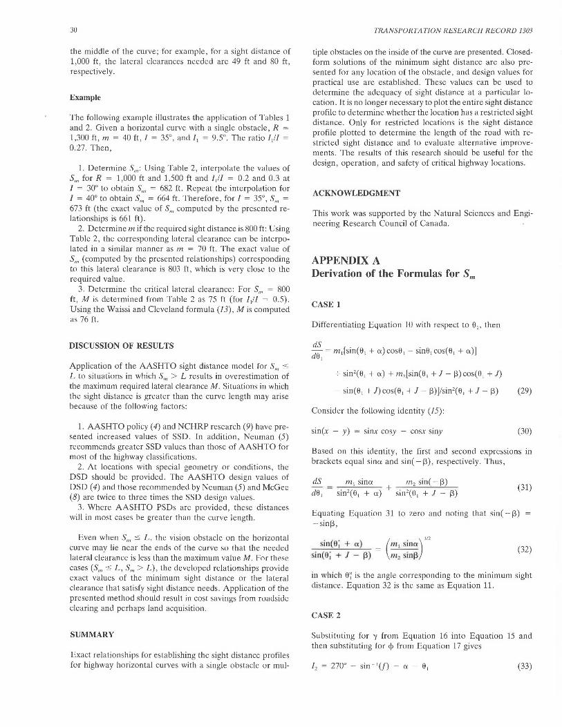
APPENDIX A Derivation of the Formulas for Sm

CASE 1

Differentiating Equation 10 with respect to 01, then

-o- sin2(0 1 +ex)+ m,[sin(0 1 + J - f3)cos(0 1 + J)

- sin(8 1 + J)cos(e, + J - f3)]/sin 2(e, + J - f3) (29)

Consider the following identity (15):

sin(x - y) = sinx cosy - cosx siny (30)

Based on this identity, the first and second expressions in brackets equal sinex and sin( - f3), respectively. Thus,

m 1 sinex m2 sin( - f3) sin2(8 1 + ex) + sin2(0 1 + J - f3)

(31)

Equating Equation 31 to zero and noting that sin( - f3) - sinf3,

si11(0; + Cl) in(o; + J - 13) ( )

112

= m 1 s'.ncx ma sm!)

(32)

in which Bi is the angle corresponding to the minimum sight distance. Equation 32 is the same as Equation 11.

CASE 2

Substituting for '{ from Equation 16 into Equation 15 and then substituting for <!> from Equation 17 gives

12 = 270° - sin~'(f) - ex - e, (33)

Easa

where f is a function of 01 given by

f = ( R ~ m) sin(J1 + a + 01 - 90°) (34)

Substituting for / 2 from Equation 33 into Equation 18 and differentiating Equation 18 with respect to 01,

-!' (1 - !2)112

m1sin(0 1 + ex) cos01 + sin2(0 1 + ex)

m1sin8 1 cos(01 + ex) _ 1

sin2(01 + ex)

where f' equals df/d0 1, which is given by

(R - m) f' = --R- sin(01 + ex + / 1)

(35)

(36)

The expression in brackets in Equation 35 equals sinex based on the identity of Equation 30. Substituting for f and f' from Equations 34 and 36 into Equation 35 and equating dS/d0 1 to zero gives

m 1 sincx

R sin2 (0; + ex)

(R - m) sin(0; + a + /1) 1 (37)

which is Equation 19.

CASE3

Equation 23 is written as

(38)

where f is a function of / 3 given by

f = [R(l - cos/3) - m]!(R sin/3) (39)

Differentiating Equation 38 with respect to 13 ,

dS [ f' ] d/3 = 2R 1 - (1 + f2) (40)

where f' = df/d/3 , which is given by

, (R sin/3 )2

- [R(l - cos/3) - m]R cos/3

f = R2 sin2/3

(41)

Substituting for f and f' from Equations 39 and 41 into Equa­tion 40 and equating dS!dl 3 to zero gives

[R(l - cos/;) - m]2

+ (R(l - cosI;) - m]R cosI; 0 (42)

31

After rearranging, Equation 42 becomes

(R(l - cos/;) - m](R - m) = 0 (43)

which is Equation 24.

APPENDIX B Numerical Solution of Equations 11 and 19

The critical angle 0i of Equations 11 and 19 can be obtained by successive approximations using the method of linear in­terpolation (16). Equation 11 or 19 is written as

f(u) = 0 (44)

where u is used instead of Si. To determine the root of Equation 44, select two values u1 and u2 for which f(u 1) and f(u 2) have opposite signs. The following steps are then performed:

1. Set

112 - 11, U3 = Uz - f ( U2) f( ) f( )

112 - 11 1

2. Iff(u3 ) has an opposite sign tof(u 1), set u2 = u3 . Other­wise, set u, = u3

3. Repeat Steps 1 and 2 until

where £ 1 and £ 2 are specified tolerance values. This method guarantees convergence. A modified linear

interpolation method, which converges faster, may also be used (/6).

REFERENCES

1. A Policy on Sight Distance for Highways, Policies on Geometric Highway Design. AASHO , Washington, D.C., 1940.

2. A Policy 011 Geometric Design of Rural Highways. AASHO, Washington, D.C., 1965.

3. A Policy on Design Standards for Stopping Sight Distance. AASHO, Washington, D.C., 1971.

4. A Policy on Geometric Design of Highways and Streets. AASHTO, Washington, D.C., 1984.

5. T . R. Neuman. New Approach to Design for Stopping Sight Distance. In Transportation Research Record 1208. TR8, Na­tional Research Council, Washington, D.C., 1989, pp. 14-22.

6. D. W. Harwood and J. C. Glennon. Passing Sight Distance De­sign for Passenger Cars and Trucks. In Transporta1io11 Research Record 1208, TRB, National Research Council, Washington, D.C., 1989, pp. 59-69.

7. J. C. Glennon. New and Improved Model of Passing Sight Dis­tance on Two-Lane Highways. In Transportation Research Rec­ord 1195, TRB, National Research Council , Washington, D.C., 1988, pp. 132-137.

8. H. W. McGee. Reevaluation of the Usefulness and Application of Decision Sight Distance. In Transporlation Research Record 1208, TRB, National Research Council, Washington, D.C., 1989, pp. 85-89.

32

9. P. L. Olson, D . E. Cleveland, P. S. Fancher, L. P. Kostyniuk, and L. W. Schneider. NCH RP Report 270: Parameters Affecting Stopping Sight Distance. TRB, National Research Council, Washington, D.C., 1984.

10. T. R. Neuman and J. C. Glennon. Cost-Effectiveness of Im ­provements to Stopping Sight Distance . In Transportation Re­search Record 923, TRB, National Research Council, Washing­ton, D.C., 1984, pp. 26-34.

11. J. C. Glennon . Effects of Sight Distance on Highway Safety. In State-of-the-Art Report 6, TRB, National Research Council, Washington, D .C., 1987, pp . 64-77 .

12. W. L. Raymond. Offsets to Sight Obstructions Near the Ends of Horizontal Curves. Civil Engineering , Vol. 42, No. 1, 1972, pp. 71-72.

13. G. R. Waissi and D. E. Cleveland. Sight Distance Relationships

TRANSPORTATION RESEARCH RECORD 1303

Involving Horizontal Curves. In Transportation Research Record 1122, TRB, National Research Council, Washington, D.C. , 1987, pp. 96-107.

14. T. R. Neuman, J. C. Glennon, and J. E. Leish. Stopping Sight Distance-An Operational and Cost Effectiveness Analysis. Re­port FHWA/RD-83/067. FHWA, U.S. Department of Trans­portation, Washington, D.C., 1982.

15. S. I. Grossman. Calculus. Academic Press, New York, N.Y. 1981.

16. C. F. Gerald and P. 0. Wheatley . Applied Numerical Analysis . Addison-Wesley Publishing Company, London, England, 1985.

Publication of this paper sponsored by Cammi/lee on Geometric Design.