Laser altimetry reveals complex pattern of GreenlandIce Sheet dynamicsBeata M. Csathoa,1, Anton F. Schenka, Cornelis J. van der Veenb, Gregory Babonisa, Kyle Duncana,Soroush Rezvanbehbahanic, Michiel R. van den Broeked, Sebastian B. Simonsene, Sudhagar Nagarajanf,and Jan H. van Angelend

aDepartment of Geology, University at Buffalo, Buffalo, NY 14260; Departments of bGeography and cGeology, University of Kansas, Lawrence, KS 66045;dInstitute for Marine and Atmospheric Research, Utrecht University, 3584 CC Utrecht, The Netherlands; eDivision of Geodynamics, DTU Space, NationalSpace institute, DK-2800 Kgs. Lyngby, Denmark; and fDepartment of Civil, Environmental and Geomatics Engineering, Florida Atlantic University, Boca Raton,FL 33431

Edited* by Ellen S. Mosley-Thompson, The Ohio State University, Columbus, OH, and approved November 17, 2014 (received for review June 23, 2014)

We present a new record of ice thickness change, reconstructed atnearly 100,000 sites on the Greenland Ice Sheet (GrIS) from laseraltimetry measurements spanning the period 1993–2012, parti-tioned into changes due to surface mass balance (SMB) and icedynamics. We estimate a mean annual GrIS mass loss of 243 ±18 Gt·y−1, equivalent to 0.68 mm·y−1 sea level rise (SLR) for 2003–2009. Dynamic thinning contributed 48%, with the largest ratesoccurring in 2004–2006, followed by a gradual decrease balancedby accelerating SMB loss. The spatial pattern of dynamic mass losschanged over this time as dynamic thinning rapidly decreased insoutheast Greenland but slowly increased in the southwest, north,and northeast regions. Most outlet glaciers have been thinningduring the last two decades, interrupted by episodes of decreasingthinning or even thickening. Dynamics of the major outlet glaciersdominated the mass loss from larger drainage basins, and simulta-neous changes over distances up to 500 km are detected, indicatingclimate control. However, the intricate spatiotemporal pattern ofdynamic thickness change suggests that, regardless of the forcingresponsible for initial glacier acceleration and thinning, the re-sponse of individual glaciers is modulated by local conditions. Re-cent projections of dynamic contributions from the entire GrIS toSLR have been based on the extrapolation of four major outletglaciers. Considering the observed complexity, we question howwell these four glaciers represent all of Greenland’s outlet glaciers.

Greenland Ice Sheet | laser altimetry | mass balance | ice dynamics

Comprehensive monitoring of the Greenland Ice Sheet (GrIS)by satellite observations has revealed increasing mass loss

since the late 1990s (1, 2), reaching 263 ± 30 Gt·y−1 for theperiod 2005–2010 (3). This translates to a sea level rise (SLR) of0.73 mm·y−1, about half of which is attributed to a decrease inSurface Mass Balance (SMB) (4) that is expected to continuethroughout this century and beyond (5). Over this period, icedynamic changes contributed about equally to total mass loss,but extrapolating this trend over the next century or two is muchmore uncertain because of the incomplete understanding of thephysical forcing mechanisms responsible for observed flow ac-celeration and thinning of marine-terminating outlet glaciers.For example, the speedup of Jakobshavn Isbræ, which started inthe late 1990s, has been attributed to the disintegration of thefloating tongue and loss of buttressing (6), triggered by increasedbasal melt due to the intrusion of warm water into the fjord (7),or to the weakening of the ice in the lateral shear margins andperhaps a change in the properties at the bed (8).Acknowledging that such predictions are at a “fairly early

stage,” the Fifth Assessment Report, issued by the Intergovern-mental Panel on Climate Change, includes a projected total SLRby 2100 of 14–85 mm, attributed to dynamic changes of the GrISfor the different future warming scenarios (5). This estimate isbased on modeled evolution of four key outlet glaciers (Jakobshavn,Helheim, Kangerlussuaq, and Petermann), whose projected

response is scaled up to all Greenland outlet glaciers (9–11).There are two concerns with this approach. First, understandingthe dynamic response of marine-terminating outlet glaciers toa warming climate—a prerequisite for deriving reliable massbalance projections—remains a major challenge (12–14). Sec-ond, considering the complexity of recent behavior of outletglaciers (15, 16), it is far from clear how four well-studied glaciersrepresent all of Greenland’s outlet glaciers and whether theirresponse can be scaled up to the entire ice sheet. For example, insoutheast Greenland, a region that accounted for more than halfof the total 2005 GrIS mass loss (17), many outlet glaciers rapidlyadjusted to a new equilibrium by 2006 (16, 18). At the same time,dynamic mass loss continued, or even accelerated, from Jakob-shavn Isbræ, the northwest Greenland outlet glaciers and theNorth East Greenland Ice Stream (19–21).For improving ice sheet models and sea-level predictions, it

is imperative to quantitatively investigate dynamic ice loss pro-cesses. Recent results from the Gravity Recovery and ClimateExperiment (GRACE) satellite gravimetry (22, 23) and input−output method (IOM, SMB minus discharge) (24) revealed aspatially shifting pattern of annual mass loss during 2003–2010,attributed to a regionally variable interplay of ocean and surfaceprocesses as well as ice dynamics. However, the limited spatialresolution of these techniques does not permit documentingthe spatial pattern of changes on individual glaciers. Preciseelevation measurements, combined with SMB estimates, offer apossibility to increase the spatial resolution of the ice sheet

Significance

We present the first detailed reconstruction of surface eleva-tion changes of the Greenland Ice Sheet from NASA’s laser al-timetry data. Time series at nearly 100,000 locations allow thecharacterization of ice sheet changes at scales ranging fromindividual outlet glaciers to larger drainage basins and theentire ice sheet. Our record shows that continuing dynamicthinning provides a substantial contribution to Greenland massloss. The large spatial and temporal variations of dynamic massloss and widespread intermittent thinning indicate the com-plexity of ice sheet response to climate forcing, strongly en-forcing the need for continued monitoring at high spatial reso-lution and for improving numerical ice sheet models.

Author contributions: B.M.C. designed research; B.M.C., A.F.S., G.B., K.D., S.R., and S.N.performed research; A.F.S., M.R.v.d.B., S.B.S., and J.H.v.A. contributed new data/analytic tools; B.M.C., C.J.v.d.V., G.B., and S.R. analyzed data; and B.M.C., A.F.S., and C.J.v.d.V.wrote the paper.

The authors declare no conflict of interest.

*This Direct Submission article had a prearranged editor.

Freely available online through the PNAS open access option.1To whom correspondence should be addressed. Email: bcsatho@buffalo.edu.

This article contains supporting information online at www.pnas.org/lookup/suppl/doi:10.1073/pnas.1411680112/-/DCSupplemental.

18478–18483 | PNAS | December 30, 2014 | vol. 111 | no. 52 www.pnas.org/cgi/doi/10.1073/pnas.1411680112

elevation change and ice dynamics records. Repeat altimetry andstereo imaging have long been used to monitor the cryosphere,mostly for mapping multiyear average elevation changes (2, 25,26), but neglecting the reconstruction of detailed temporal his-tories. As surface elevation observations are often collectedwith varying spatial resolutions and at slightly different loca-tions, the derivation of accurate elevation histories has remaineda challenging task.Here we present, to our knowledge, the first detailed recon-

struction of GrIS elevation changes, derived from NASA’s 1993–2012 laser altimetry record. Available at nearly 100,000 locationsand partitioned into thickness changes associated with SMBvariations and dynamic processes, our elevation change historycharacterizes ice sheet processes on spatial scales ranging fromindividual outlet glaciers to larger drainage basins and the entireice sheet. By retaining the original temporal resolution, it issuitable for investigating rapid ice dynamic responses to con-temporary atmospheric and oceanic forcings, processes that arestill poorly understood (13, 14). Our reconstruction reveals thecomplexity of ice sheet response to climate forcing. We detectsimilar, simultaneous elevation changes over distances up to 500km, indicating climate control on recent mass changes. However,we also show that outlet glacier dynamics exhibits large spatio-temporal variability, suggesting that the response of individualoutlet glaciers likely depends on local conditions, such as bedtopography and local climate conditions.

ResultsReconstruction of GrIS Elevation Change. As part of NASA’s Pro-gram for Arctic Regional Climate Assessment (PARCA), airbornelaser altimetry surveys began in 1993 with NASA’s Airborne To-pographic Mapper (ATM) (27). However, investigations of icesheet mass balance and related sea level rise were hamperedby the lack of spatially comprehensive elevation time series. Toremedy this, NASA launched the Ice, Cloud and land ElevationSatellite (ICESat) mission in 2003 with the primary goal of mea-suring elevation changes over the polar ice sheets with sufficientaccuracy to assess their impact on global sea level (28). After asuccessful period of obtaining accurate elevations of the Greenlandand Antarctic ice sheets, ICESat’s last campaign ended on Oc-tober 11, 2009. The successor, ICESat-2, is expected to belaunched in 2017. To “bridge” the intervening time withoutsatellite laser altimetry data, NASA started Operation IceBridge

mission (OIB), which has been gathering laser altimetry datausing the ATM and the Land, Vegetation and Ice Sensor [LVIS(29)] airborne systems in both polar regions.We developed the novel Surface Elevation Reconstruction

and Change detection (SERAC) method to determine surfaceelevation changes at ICESat crossover areas (intersections ofascending and descending ICESat tracks) (30). The method isbased on fitting an analytical function to the laser points of asurface patch, such as a crossover area, of ∼1 km2 in size. Thesurface patches of different time epochs at the same crossoverarea are related to each other; we have introduced the constraintthat within a surface patch, the shape of the ice sheet remains thesame over the entire observation period; only its absolute ele-vation changes. The least-squares adjustment of SERAC simul-taneously determines one set of best-fit shape parameters anda time series of elevations for all time epochs involved, togetherwith rigorous error estimates (ref. 30, SI Text, and Fig. S1).Originally limited to ICESat crossover areas only, SERAC has

been extended to provide solutions along the ICESat groundtracks by combining ICESat data with airborne laser altimetrydata (31). In this way, the spatial density of surface elevationtime series increases dramatically, as Fig. 1 vividly demonstrates.Fig. 1B depicts ICESat crossover locations (brown) and addi-tional locations where 2003–2009 ATM and LVIS flights inter-sected or repeated ICESat ground tracks (blue). However, largegaps remain, especially in southern Greenland. Adding ATMdata from the period 1993–2002 as well as ATM and LVIS datafrom 2010 to 2012 remedies this situation, resulting in a densedata set.The fusion framework of SERAC offers other advantages. For

example, inclusion of ATM and/or LVIS data that were collectedduring ICESat mission (2003−2009) increases the temporal reso-lution of the elevation change record. If data are available fromearlier time periods, the time series are extended backward intime, before 2003. Using data from the OIB mission extends thetime series toward the present.Ultimately, by combining all NASA laser altimetry measure-

ments, elevation time series are reconstructed at ∼100,000locations, resulting in a very dense coverage along ICESatground tracks, especially in the ice sheet marginal region. Despiteoccasional cloud cover, ice sheet elevations were measured atleast once during each of the 19 ICESat operational periods atmost crossover locations (30). Thus, by adding ATM and LVIS

A B C D

Fig. 1. Location of GrIS elevation time series according to the main data sets used for SERAC reconstruction. (A) PARCA ATM (1993−2003) and ICESat(purple); (B) PARCA ATM (2003−2009) and ICESat (blue), ICESat crossovers only (brown); (C) OIB ATM/LVIS (2009−2012) and ICESat (red); and (D) combined: allsolutions (black). GrIS is shown in gray, and land surface with local ice caps and glaciers is in green/brown hues. Symbols in D mark the locations of elevationchange time series shown in Fig. S1.

Csatho et al. PNAS | December 30, 2014 | vol. 111 | no. 52 | 18479

EART

H,A

TMOSP

HER

IC,

ANDPL

ANET

ARY

SCIENCE

S

measurements, a dense temporal sampling is obtained for 2003–2009, with additional points from LVIS and ATM extendingmost of the curves beyond ICESat’s lifetime (Fig. 2A and Fig. S1).After removing the effect of vertical crustal motion due to GlacialIsostatic Adjustment (GIA; SI Text), we partition the ice thicknesschange time series into components associated with ice dynamicsand SMB changes (Materials and Methods, SI Text, and Fig. S1).The high spatial density of the new 1993–2012 elevation

change record and the 91-d repeat cycle of ICESat allow for theinvestigation of the spatiotemporal pattern of ice sheet thicknesschange at different scales. The ice thickness change time series(Fig. 2A and Fig. S1) provides the highest resolution, suitable forcharacterizing the dynamic processes affecting individual outletglaciers. The most recent compilation of GrIS ice velocities includes242 outlet glaciers with a width greater than 1.5 km (32). Weidentified 130 of these glaciers with a 5- to 19-y-long altimetryrecord, out of which 115 are marine terminating (Tables S1 andS2). Average elevation change rates are found to be in goodagreement with previous studies (SI Text and Table S3). However,

we have shown that changes are typically nonlinear in time andmost of the rapid changes occur during the ICESat mission (Fig.2A). For many marine-terminating outlet glaciers, dynamicthickness change patterns are consistent with an inland propaga-tion of dynamic thinning or thickening initiated at the coast (Fig.S2 A and B). Some glaciers exhibit a more complicated behavior,however. For example, Størstrommen, L. Bistrup Bræ, and MarieSophie glaciers, which are quiescent surging glaciers, have a char-acteristic pattern with large, steady thickening at their sourceregions, as ice accumulates upstream of the reduced flow, andthinning below the area where the surge was initiated (Fig. S2Cand Table S1), while the complex elevation change pattern ofHagen Bræ might indicate an ongoing surge (Table S1). Short-term, sometimes cyclic elevation changes occurred on 15 outletglaciers, all marine terminating (SI Text and Table S1), and mayindicate control from subglacial hydrology or are perhaps relatedto the drainage of proglacial lakes (e.g., Daugaard-JensenGlacier, Fig. S2D). Dynamic thinning was negligible on 13 out ofthe 15 land-terminating glaciers (SI Text and Tables S1 and S2).

Fig. 2. Classification of outlet glaciers based on dynamic thickness change pattern. (A) Thickness change time series derived from the combined ICESat/ATM/LVIS altimetry record (1993−2012) illustrating different dynamic outlet glacier behaviors. Thickening: Store Glacier (6); no dynamic change: Petermann Glacier(78); decelerating thinning: Kjer Glacier (83); accelerating thinning: Zachariæ Isstrom (51) and Ikertivaq NN (46); full cycle thinning: Jakobshavn Isbræ (1);thinning with varying rate: Midgård Glacier (121); thinning, thickening, and thinning with abrupt termination of initial thinning: Helheim (3), Koge Bugt C (4),and A. P. Bernstorff (12) glaciers; unique pattern with periodic thinning and thickening: Daugaard-Jensen Glacier (8). Numbers in parentheses are ID numbersfrom ref. 32 and in Table S1. Gray box marks the duration of the ICESat mission, and glacier locations are shown in B. Dynamic thickness changes of the fourlarge outlet glaciers, Jakobshavn Isbræ, Kangerlussuaq, Helheim, and Petermann glaciers, underlined in the figure, are modeled in refs. 9–11. (B) Distribution ofdifferent outlet glacier behavior types over a background of ice sheet bed elevation from ref. 45. Inset shows the detailed pattern north of Jakobshavn Isbræoverlain on ice velocities from ref. 32. Abbreviations mark the following outlet glaciers: Sermeq Avannarleq (SA, 53), Sermeq Kujalleq (SK, 13), KangilerngataSermia (KS, 52), Eqip Sermia (ES, 90), Kangiata Nunaata Sermia (KNS, 36), Skinfaxe (S, 82), Rimfaxe (R, 58), and Heimdal (H, 39) glaciers. See Table S1 fora complete list of glaciers and their classification based on 2003–2009 and 1993–2012 dynamic thickness change patterns.

18480 | www.pnas.org/cgi/doi/10.1073/pnas.1411680112 Csatho et al.

To facilitate interpretation, glaciers are divided into the follow-ing distinct groups according to their dynamic thickness changepattern in 2003–2009: thinning with steady or slowly changingrates (accelerating, decelerating, full cycle thinning); slow orrapid thinning that abruptly terminated and was followed bythickening and in some cases by resumed thinning; thickening;unique elevation change pattern; and no dynamic change (Fig. 2and Table S1).To investigate drainage basin-scale processes, we compute

annual ice thickness change rates at each surface patch locationfrom a polynomial fit through the thickness changes recon-structed by SERAC (30) and partition these rates into changesassociated with SMB and ice dynamics (Materials and Methods,SI Text, and Fig. S1). The interpolated annual thickness changerate grids show intricate and rapidly changing patterns (Fig. 3and Movie S1). To quantify these, volume and mass change ratesof the main ice sheet regions are calculated (Fig. 4 and TablesS4 and S5).

GrIS Ice Thickness Change and Mass Loss Patterns, 1993–2012. Weestimated a mean annual GrIS loss of 243 ± 18 Gt·y−1 (277 ± 7km3·y−1), equivalent to 0.68 ± 0.05 mm·y−1 SLR for 2003–2009(Tables S4 and S5). This mass loss and its interannual variabilityare in good agreement with the reconciled GrIS mass loss esti-mate derived from a combined ensemble of laser altimetry,GRACE, and IOM data (3). However, we detected higheraverage mass loss and interannual variability than the laser al-timetry results included in ref. 3, bringing the laser altimetry,GRACE, and IOM estimates closer to each other (ref. 3, SI Text,and Tables S5 and S6), thus reconciling the previously perceivedinconsistencies among different methods. Dynamic thinning con-tributed 48% to the total mass loss, which is the same as reportedin ref. 4. Dynamic loss was largest in 2004–2005, followed bya gradual decrease that was balanced by accelerating SMB loss(Fig. 4). However, at the same time, the relative contributions ofmajor drainage basins changed significantly (Figs. 3 and 4), in-dicating that processes acting on time scales of less than a decade

have a significant effect on ice sheet mass loss and related SLR.The only region exhibiting steady mass loss from 2003 to 2009was Jakobshavn, while mass loss decelerated from southeast andeast Greenland and accelerated from the rest of Greenland,confirming the pattern reconstructed from GRACE observations(23). In this section, we review the dynamic behavior of indi-vidual marine-terminating outlet glaciers and explore their impacton drainage basin scale dynamic mass changes.Almost half of the total 2003–2009 GrIS mass loss originated

from southeast Greenland (Table S5). Glaciers in this sectorthinned rapidly between 2003 and 2005, reaching their peakdischarge in 2005 (refs. 16 and 18, Figs. 3 and 4). During thistime, dynamic thinning extended far inland, up to the ice dividein some areas (Movie S1), maintaining a pattern that startedin the 1970s or earlier (33). This large dynamic loss, peaking at166 ± 31 Gt·y−1, was a major source of the record negative GrISmass balance of 293 ± 38 Gt·y−1 in 2004–2005. As flow accelerationslowed down or reversed to deceleration after 2005 (16), thin-ning rates decreased, and several glaciers, for example HelheimGlacier, started to thicken (Fig. 2). At the same time, the long-term trend of high-elevation thinning also reversed, and by 2007–2008, most of southeast GrIS exhibited dynamic thickening (Fig.3 and Movie S1). By 2007–2008, the ice loss rate from thesoutheast GrIS dropped to less than one third of its peak value,as a result of a diminishing dynamic mass loss. However, theslowdown and thickening of outlet glaciers was short lived, asthey resumed acceleration (16) and thinning by 2009 (Fig. 2).In addition to widespread short-term changes, outlet glacierthinning shows a large spatial variability in southeast Greenland,much like the velocity record (16), indicating an intricate in-terplay of regional and local forcings and controls. For example,rapid thickening of outlet glaciers within a region extending to500 km in north−south direction, and including Helheim,Køge Bugt C, and A. P. Bernstorff glaciers, started at the sametime and exhibited very similar patterns (Fig. 2), suggesting re-gional climate controls. Meanwhile, other glaciers in the region,such as Midgård and Ikertivaq glaciers, continued to thin, losing

Fig. 3. Annual total, SMB-related, and ice dynamics-related thickness change rates of the GrIS for 2003–2009 balance years from ICESat, ATM and LVIS laseraltimetry observations (see Fig. 1 for locations of el-evation change records). Dotted lines on the dynamicthickness change maps mark the ELA (average 2003–2009 SMB = 0). Ice sheet boundary is from ref. 46, andblack regions show weakly or not connected glaciersand ice caps. Balance years start on September 1 andend on August 31 of the following year. See Movie S1for a higher-resolution, animated version of the figure.

Csatho et al. PNAS | December 30, 2014 | vol. 111 | no. 52 | 18481

EART

H,A

TMOSP

HER

IC,

ANDPL

ANET

ARY

SCIENCE

S

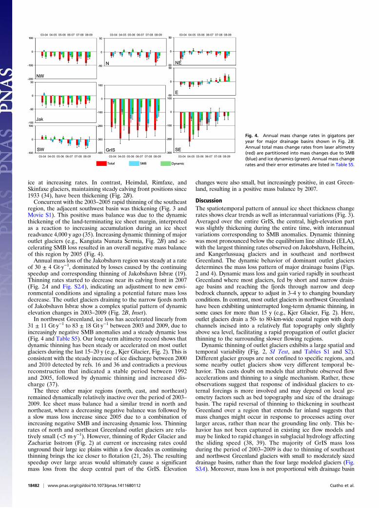
ice at increasing rates. In contrast, Heimdal, Rimfaxe, andSkinfaxe glaciers, maintaining steady calving front positions since1933 (34), have been thickening (Fig. 2B).Concurrent with the 2003–2005 rapid thinning of the southeast

region, the adjacent southwest basin was thickening (Fig. 3 andMovie S1). This positive mass balance was due to the dynamicthickening of the land-terminating ice sheet margin, interpretedas a reaction to increasing accumulation during an ice sheetreadvance 4,000 y ago (35). Increasing dynamic thinning of majoroutlet glaciers (e.g., Kangiata Nunata Sermia, Fig. 2B) and ac-celerating SMB loss resulted in an overall negative mass balanceof this region by 2005 (Fig. 4).Annual mass loss of the Jakobshavn region was steady at a rate

of 30 ± 4 Gt·y−1, dominated by losses caused by the continuingspeedup and corresponding thinning of Jakobshavn Isbræ (19).Thinning rates started to decrease near its calving front in 2007(Fig. 2A and Fig. S2A), indicating an adjustment to new envi-ronmental conditions and signaling a potential future mass lossdecrease. The outlet glaciers draining to the narrow fjords northof Jakobshavn Isbræ show a complex spatial pattern of dynamicelevation changes in 2003–2009 (Fig. 2B, Inset).In northwest Greenland, ice loss has accelerated linearly from

31 ± 11 Gt·y−1 to 83 ± 18 Gt·y−1 between 2003 and 2009, due toincreasingly negative SMB anomalies and a steady dynamic loss(Fig. 4 and Table S5). Our long-term altimetry record shows thatdynamic thinning has been steady or accelerated on most outletglaciers during the last 15–20 y (e.g., Kjer Glacier, Fig. 2). This isconsistent with the steady increase of ice discharge between 2000and 2010 detected by refs. 16 and 36 and contradicts a previousreconstruction that indicated a stable period between 1992and 2005, followed by dynamic thinning and increased dis-charge (37).The three other major regions (north, east, and northeast)

remained dynamically relatively inactive over the period of 2003–2009. Ice sheet mass balance had a similar trend in north andnortheast, where a decreasing negative balance was followed bya slow mass loss increase since 2005 due to a combination ofincreasing negative SMB and increasing dynamic loss. Thinningrates of north and northeast Greenland outlet glaciers are rela-tively small (<5 m·y−1). However, thinning of Ryder Glacier andZachariæ Isstrom (Fig. 2) at current or increasing rates couldunground their large ice plains within a few decades as continuingthinning brings the ice closer to flotation (21, 26). The resultingspeedup over large areas would ultimately cause a significantmass loss from the deep central part of the GrIS. Elevation

changes were also small, but increasingly positive, in east Green-land, resulting in a positive mass balance by 2007.

DiscussionThe spatiotemporal pattern of annual ice sheet thickness changerates shows clear trends as well as interannual variations (Fig. 3).Averaged over the entire GrIS, the central, high-elevation partwas slightly thickening during the entire time, with interannualvariations corresponding to SMB anomalies. Dynamic thinningwas most pronounced below the equilibrium line altitude (ELA),with the largest thinning rates observed on Jakobshavn, Helheim,and Kangerlussuaq glaciers and in southeast and northwestGreenland. The dynamic behavior of dominant outlet glaciersdetermines the mass loss pattern of major drainage basins (Figs.2 and 4). Dynamic mass loss and gain varied rapidly in southeastGreenland where most glaciers, fed by short and narrow drain-age basins and reaching the fjords through narrow and deepbedrock channels, appear to adjust in 3–4 y to changing boundaryconditions. In contrast, most outlet glaciers in northwest Greenlandhave been exhibiting uninterrupted long-term dynamic thinning, insome cases for more than 15 y (e.g., Kjer Glacier, Fig. 2). Here,outlet glaciers drain a 50- to 80-km-wide coastal region with deepchannels incised into a relatively flat topography only slightlyabove sea level, facilitating a rapid propagation of outlet glacierthinning to the surrounding slower flowing regions.Dynamic thinning of outlet glaciers exhibits a large spatial and

temporal variability (Fig. 2, SI Text, and Tables S1 and S2).Different glacier groups are not confined to specific regions, andsome nearby outlet glaciers show very different temporal be-havior. This casts doubt on models that attribute observed flowaccelerations and thinning to a single mechanism. Rather, theseobservations suggest that response of individual glaciers to ex-ternal forcings is more involved and may depend on local ge-ometry factors such as bed topography and size of the drainagebasin. The rapid reversal of thinning to thickening in southeastGreenland over a region that extends far inland suggests thatmass changes might occur in response to processes acting overlarger areas, rather than near the grounding line only. This be-havior has not been captured in existing ice flow models andmay be linked to rapid changes in subglacial hydrology affectingthe sliding speed (38, 39). The majority of GrIS mass lossduring the period of 2003–2009 is due to thinning of southeastand northwest Greenland glaciers with small to moderately sizeddrainage basins, rather than the four large modeled glaciers (Fig.S3A). Moreover, mass loss is not proportional with drainage basin

Fig. 4. Annual mass change rates in gigatons peryear for major drainage basins shown in Fig. 2B.Annual total mass change rates from laser altimetry(red) are partitioned into mass changes due to SMB(blue) and ice dynamics (green). Annual mass changerates and their error estimates are listed in Table S5.

18482 | www.pnas.org/cgi/doi/10.1073/pnas.1411680112 Csatho et al.

area (Fig. S3B), as was assumed by ref. 10. These findings challengethe practice of estimating the future dynamic contribution of theentire GrIS to global sea level based on modeled behavior of threeor four major outlet glaciers, one of which (Petermann Glacier) didnot show much dynamic change over the period considered.Our record shows that continuing dynamic thinning provides

a substantial contribution to Greenland mass loss. The largespatial and temporal variations of dynamic mass loss and wide-spread intermittent thinning indicate the complexity of ice sheetresponse to climate forcing, pointing to the need for continuedmonitoring of the GrIS at high spatial resolution.

Materials and MethodsElevation change time series are reconstructed from ICESat, ATM, and LVISlaser altimetry data by SERAC (see SI Text for details on the data sets andtheir accuracies). They are corrected for GIA and partitioned into compo-nents corresponding to SMB anomalies, changes in firn compaction rates,and ice dynamics (Fig. S1). GIA-related vertical crustal motion estimatesare from ref. 40. Regional Atmospheric Climate Model (RACMO2/GR) SMBanomalies (41) are converted into ice thickness change using surface firndensities derived by a simple empirical model (42). This model accounts forthe formation of ice lenses in the snowpack assuming that all retained

meltwater refreezes at the same annual layer. Variations of firn compactionrates are from a 5-km by 5-km gridded model (43) forced by the output fromthe HIRHAM5 Regional Climate Model (44). Annual rates of total, SMB-related, and dynamic ice thickness change rates are estimated from polynomialapproximations of the time series, and are gridded into 2-km-resolution gridsusing ordinary kriging with an exponential, isotropic variogram model. Toobtain mass changes, we converted dynamic thickness changes to masschanges with an assumed ice density of 917 kg·m−3. Total mass changeswere then estimated as the sum of dynamic and SMB mass changes. Detailson the computation of the total, SMB, and dynamic thickness change timeseries, as well as thickness, volume, and mass change rates, together with theirerror estimates, are presented in SI Text. Comparison with published thicknesschange rates (Table S3) and mass balance rate estimates (Table S6) confirmsthe accuracy of our results.

ACKNOWLEDGMENTS. ICESat, ATM, and LVIS data were collected by NASA’sPARCA, ICESat, and OIB missions and distributed by the National Snow andIce Data Center. B.M.C., A.F.S., C.J.v.d.V., K.D., G.B., S.R., and S.N. acknowledgesupport by NASA’s Polar Program under Grants NNX10AV13G, NNX11AR23G,and NNX12AH15G. M.R.v.d.B. and J.H.v.A. acknowledge support from theNetherlands Polar Program of Netherlands Organization for Scientific Re-search Division for the Earth and Life Sciences (NWO-ALW) and EU FP7program ice2sea.

1. Rignot E, Velicogna I, van den Broeke MR, Monaghan A, Lenaerts J (2011) Accelera-tion of the contribution of the Greenland and Antarctic ice sheets to sea level rise.Geophys Res Lett 38(5):L05503.

2. Zwally HJ, et al. (2011) Greenland ice sheet mass balance: Distribution of increasedmass loss with climate warming; 2003-07 versus 1992-2002. J Glaciol 57(201):88–102.

3. Shepherd A, et al. (2012) A reconciled estimate of ice-sheet mass balance. Science338(6111):1183–1189.

4. van den Broeke M, et al. (2009) Partitioning recent Greenland mass loss. Science326(5955):984–986.

5. Church JA, et al. (2013) Sea level change. Climate Change 2013: The Physical ScienceBasis. Contribution of Working Group I to the Fifth Assessment Report of the In-tergovernmental Panel on Climate Change, eds Stocker TF, et al. (Cambridge UnivPress, New York), pp 1137−1216.

6. Joughin I, et al. (2008) Continued evolution of Jakobshavn Isbrae following its rapidspeedup. J Geophys Res 113(F4):F04006.

7. Holland DM, Thomas RH, De Young B, Ribergaard MH, Lyberth B (2008) Accelerationof Jakobshavn Isbrtriggered by warm subsurface ocean waters.Nat Geosci 1(10):659–664.

8. van der Veen CJ, Plummer JC, Stearns LA (2011) Controls on the recent speed-up ofJakobshavn Isbræ, West Greenland. J Glaciol 57(204):770–782.

9. Price SF, Payne AJ, Howat IM, Smith BE (2011) Committed sea-level rise for the nextcentury from Greenland ice sheet dynamics during the past decade. Proc Natl Acad SciUSA 108(22):8978–8983.

10. Nick FM, et al. (2013) Future sea-level rise from Greenland’s main outlet glaciers ina warming climate. Nature 497(7448):235–238.

11. Goelzer H, et al. (2013) Sensitivity of Greenland ice sheet projections to model for-mulations. J Glaciol 59(216):733–749.

12. Joughin I, Alley RB, Holland DM (2012) Ice-sheet response to oceanic forcing. Science338(6111):1172–1176.

13. Straneo F, et al. (2013) Challenges to understanding the dynamic response ofGreenland’s marine terminating glaciers to oceanic and atmospheric forcing. Bull AmMeteorol Soc 94(8):1131–1144.

14. Straneo F, Heimbach P (2013) North Atlantic warming and the retreat of Greenland’soutlet glaciers. Nature 504(7478):36–43.

15. McFadden EM, Howat IM, Joughin I, Smith BE, Ahn Y (2011) Changes in the dynamicsof marine terminating outlet glaciers in west Greenland (2000−2009). J Geophys Res116(F2):F02022.

16. Moon T, Joughin I, Smith B, Howat I (2012) 21st-century evolution of Greenlandoutlet glacier velocities. Science 336(6081):576–578.

17. Rignot E, Kanagaratnam P (2006) Changes in the velocity structure of the GreenlandIce Sheet. Science 311(5763):986–990.

18. Howat IM, Joughin I, Scambos TA (2007) Rapid changes in ice discharge fromGreenland outlet glaciers. Science 315(5818):1559–1561.

19. Howat IM, et al. (2011) Mass balance of Greenland’s three largest outlet glaciers,2000−2010. Geophys Res Lett 38(12):L12501.

20. Khan SA, Wahr J, Bevis M, Velicogna I, Kendrick E (2010) Spread of ice mass loss intonorthwest Greenland observed by GRACE and GPS. Geophys Res Lett 37(6):L06501.

21. Khan SA, et al. (2014) Sustained mass loss of the northeast Greenland ice sheettriggered by regional warming. Nat Clim Change 4(4):292–299.

22. Harig C, Simons FJ (2012) Mapping Greenland’s mass loss in space and time. Proc NatlAcad Sci USA 109(49):19934–19937.

23. Luthcke SB, et al. (2013) Antarctica, Greenland and Gulf of Alaska land-ice evolutionfrom an iterated GRACE global mascon solution. J Glaciol 59(216):613–631.

24. Sasgen I, et al. (2012) Timing and origin of recent regional ice-mass loss in Greenland.

Earth Planet Sci Lett 333:293–303.25. Pritchard HD, Arthern RJ, Vaughan DG, Edwards LA (2009) Extensive dynamic thinning

on the margins of the Greenland and Antarctic ice sheets. Nature 461(7266):971–975.26. Thomas R, Frederick E, Krabill W, Manizade S, Martin C (2009) Recent changes on

Greenland outlet glaciers. J Glaciol 55(189):147–162.27. Krabill WB, et al. (2002) Aircraft laser altimetry measurement of elevation changes of

the Greenland ice sheet: Technique and accuracy assessment. J Geodyn 34(3):357–376.28. Zwally HJ, et al. (2002) ICESat’s laser measurements of polar ice, atmosphere, ocean,

and land. J Geodyn 34(3):405–445.29. Hofton MA, Blair JB, Luthcke SB, Rabine DL (2008) Assessing the performance of 20−

25 m footprint waveform lidar data collected in ICESat data corridors in Greenland.

Geophys Res Let 35(24):L24501.30. Schenk T, Csathó B (2012) A new methodology for detecting ice sheet surface elevation

changes from laser altimetry data. IEEE Trans Geosci Remote Sens 50(9):3302–3316.31. Schenk T, Csatho B, van der Veen C, McCormick D (2014) Fusion of multi-sensor sur-

face elevation data for improved characterization of rapidly changing outlet glaciers

in Greenland. Remote Sens Environ 149:239–251.32. Rignot E, Mouginot J (2012) Ice flow in Greenland for the International Polar Year

2008−2009. Geophys Res Lett 39(11):L11501.33. Thomas R, et al. (2001) Mass balance of higher-elevation parts of the Greenland ice

sheet. J Geophys Res 106(D24):33707–33716.34. Bjørk AA, et al. (2012) An aerial view of 80 years of climate-related glacier 278

fluctuations in southeast Greenland. Nat Geosci 5(6):427–432.35. Huybrechts P (1994) The present evolution of the Greenland ice sheet: An assessment

by modelling. Global Planet Change 9(1):39–51.36. Enderlin EM, et al. (2014) An improved mass budget for the Greenland ice sheet.

Geophys Res Lett 41(3):866–872.37. Kjær KH, et al. (2012) Aerial photographs reveal late-20th-century dynamic ice loss in

northwestern Greenland. Science 337(6094):569–573.38. Schoof C (2010) Ice-sheet acceleration driven by melt supply variability. Nature

468(7325):803–806.39. Koenig LS, Mige C, Forster RR, Brucker L (2014) Initial in situ measurements of pe-

rennial meltwater storage in the Greenland firn aquifer. Geophys Res Lett 41(1):81–85.40. G A, Wahr J, Zhong S (2013) Computations of the viscoelastic response of a 3-D

compressible Earth to surface loading: An application to Glacial Isostatic Adjustment

in Antarctica and Canada. Geophys J Int 192(2):557–572.41. van Angelen JH, van den Broeke MR, Wouters B, Lenaerts JTM (2014) Contemporary

(1960−2012) evolution of the climate and surface mass balance of the Greenland ice

sheet. Surv Geophys 35(5):1155–1174.42. Reeh N, Fisher DA, Koerner RM, Clausen HB (2005) An empirical firn-densification

model comprising ice lenses. Ann Glaciol 42(1):101–106.43. Sørensen LS, et al. (2011) Mass balance of the Greenland ice sheet (2003−2008) from ICESat

data – the impact of interpolation, sampling and firn density. Cryosphere 5(1):173–186.44. Lucas-Picher P, et al. (2012) Very high resolution regional climate model simulations

over Greenland: Identifying added value. J Geophys Res 117(D2):D02108.45. Bamber JL, et al. (2013) A new bed elevation dataset for Greenland. Cryosphere

7(2):499–510.46. Rastner P, Bolch T, Molg N, Machguth H, Paul F (2012) The first complete glacier in-

ventory for the whole of Greenland. Cryosphere 6(4):1483–1495.

Csatho et al. PNAS | December 30, 2014 | vol. 111 | no. 52 | 18483

EART

H,A

TMOSP

HER

IC,

ANDPL

ANET

ARY

SCIENCE

S