larsgaard master
TRANSCRIPT
May 2007Anne Cathrine Elster, IDI
Master of Science in Computer ScienceSubmission date:Supervisor:
Norwegian University of Science and TechnologyDepartment of Computer and Information Science
Parallelizing Particle-In-Cell Codeswith OpenMP and MPI
Nils Magnus Larsgård


Problem Description
This thesis searches for the best configuration of OpenMP/MPI for optimal performance. We willrun a parallel simulation-application on a modern supercomputer to measure the effects ofdifferent configurations of the mixed code. After analyzing the performance of differentconfigurations from a hardware point of view, we will propose a general model for estimatingoverhead in OpenMP loops.
We will parallelize a physics simulation to do large scale simulations as efficient as possible.
We will look at typical physics simulation codes to parallelize and optimize them with OpenMP andMPI in a mixed mode. The goal of the parallelization is to make the code highly efficient for aparallel system and to make it as scalable as possible to do large-scale simulations as well asusing this parallelized application as a benchmark for our MPI/OpenMP tests.
Assignment given: 20. January 2007Supervisor: Anne Cathrine Elster, IDI


Abstract
Today’s supercomputers often consists of clusters of SMP nodes. BothOpenMP and MPI are programming paradigms that can be used forparallelization of codes for such architectures.
OpenMP uses shared memory, and hence is viewed as a simplerprogramming paradigm than MPI that is primarily a distributed memoryparadigm. However, the Open MP applications may not scale beyond oneSMP node. On the other hand, if we only use MPI, we might introduceoverhead in intra-node communication.
In this thesis we explore the trade-offs between using OpenMP, MPI anda mix of both paradigms for the same application. In particular, we lookat a physics simulation and parallalize it with both OpenMP and MPI forlarge-scale simulations on modern supercomputers.
A parallel SOR solver with OpenMP and MPI is implemented and theeffects of such hybrid code are measured. We also utilize the FFTW-library that includes both system-optimized serial implementations and aparallel OpenMP FFT implementation. These solvers are used to make ourexisting Particle-In-Cell codes be more scalable and compatible with currentprogramming paradigms and supercomputer architectures.
We demonstrate that the overhead from communications in OpenMPloops on an SMP node is significant and increases with the number ofCPUs participating in execution of the loop compared to equivalent MPIimplementations. To analyze this result, we also present a simple model onhow to estimate the overhead from communication in OpenMP loops.
Our results are both surprising and should be of great interest to a largeclass of parallel applications.
i

ii

Acknowledgments
The greatest contribution to and inspiration for this work has been Dr.Anne C. Elster. Without her previous works and her well documented code,my understanding of advanced physics and fourier solvers would have beenclose to nothing. Her famous brownies every Friday has also made the HighPerformance Computing(HPC) Group at NTNU to a great place to makefriends and exchange opinions and experiences in the HPC field.
Thanks to Jan Christian Meyer for giving me his PIC codes and a goodintroduction to the field of particle simulation.
Thanks to all my friends and peers in the HPC group and the peopleat the computer-lab “Ugle” for ideas and feedback on coding concepts andtheories.
I would also give a huge thanks to the people maintaining the Njordsupercomputer at NTNU. I have not had any problems related to neithersoftware or hardware on Njord during this project.
iii

iv

Contents
Abstract i
Acknowledgments iii
1 Introduction 11.1 Motivation . . . . . . . . . . . . . . . . . . . . . . . . . . . . 1
1.1.1 Thesis Goal . . . . . . . . . . . . . . . . . . . . . . . . 11.2 Terminology . . . . . . . . . . . . . . . . . . . . . . . . . . . . 21.3 Thesis Outline . . . . . . . . . . . . . . . . . . . . . . . . . . 2
2 Background Theory 52.1 Performance Modeling . . . . . . . . . . . . . . . . . . . . . . 5
2.1.1 Amdahl’s Law . . . . . . . . . . . . . . . . . . . . . . 52.1.2 Work and Overhead . . . . . . . . . . . . . . . . . . . 62.1.3 Efficiency . . . . . . . . . . . . . . . . . . . . . . . . . 6
2.2 The Message Passing Interface - MPI . . . . . . . . . . . . . . 72.3 OpenMP . . . . . . . . . . . . . . . . . . . . . . . . . . . . . . 72.4 Hybrid Programming Models . . . . . . . . . . . . . . . . . . 8
2.4.1 Classifications . . . . . . . . . . . . . . . . . . . . . . . 82.5 Supercomputer Memory Models . . . . . . . . . . . . . . . . . 92.6 Particle-In-Cell Simulations . . . . . . . . . . . . . . . . . . . 112.7 PDE Solvers . . . . . . . . . . . . . . . . . . . . . . . . . . . . 12
2.7.1 Direct Solvers and the FFT . . . . . . . . . . . . . . . 122.7.2 Iterative Solvers and the SOR . . . . . . . . . . . . . . 13
2.8 Math Libraries . . . . . . . . . . . . . . . . . . . . . . . . . . 142.8.1 The “Fastest Fourier Transform in the West” . . . . . 142.8.2 Portable, Extensible Toolkit for Scientific Computation 15
2.9 Profilers . . . . . . . . . . . . . . . . . . . . . . . . . . . . . . 162.9.1 Software profiling: gprof, prof . . . . . . . . . . . . . . 162.9.2 Hardware profiling: pmcount . . . . . . . . . . . . . . 16
2.10 Related Work . . . . . . . . . . . . . . . . . . . . . . . . . . . 162.10.1 Hybrid Parallel Programming on HPC Platforms . . . 162.10.2 Parallelization Issues and Particle-In-Cell Codes . . . 16
v

2.10.3 Emerging Technologies Project: Cluster Technologies.PIC codes: Eulerian data Partitioning . . . . . . . . . 17
2.10.4 UCLA Parallel PIC Framework . . . . . . . . . . . . . 17
3 Particle-In-Cell Codes 193.1 General Theory . . . . . . . . . . . . . . . . . . . . . . . . . . 19
3.1.1 The Field and the Particles . . . . . . . . . . . . . . . 193.1.2 A Particles Contribution to the Field . . . . . . . . . . 203.1.3 Solving the Field . . . . . . . . . . . . . . . . . . . . . 203.1.4 Updating Speed and Position . . . . . . . . . . . . . . 21
3.2 Anne C. Elster’s Version . . . . . . . . . . . . . . . . . . . . . 213.2.1 Program Flow . . . . . . . . . . . . . . . . . . . . . . 213.2.2 An Example Run . . . . . . . . . . . . . . . . . . . . . 223.2.3 Output, Timings and Plotdata . . . . . . . . . . . . . 223.2.4 Optimization Potentials . . . . . . . . . . . . . . . . . 223.2.5 Initial Performance . . . . . . . . . . . . . . . . . . . . 23
3.3 Jan Christian Meyer’s Version . . . . . . . . . . . . . . . . . . 233.3.1 Program Flow . . . . . . . . . . . . . . . . . . . . . . 233.3.2 An Example Run . . . . . . . . . . . . . . . . . . . . . 243.3.3 Output - stderr, Timings and Plotdata . . . . . . . . . 243.3.4 Optimization Potentials . . . . . . . . . . . . . . . . . 263.3.5 Initial Performance . . . . . . . . . . . . . . . . . . . . 26
4 Optimizing PIC Codes 294.1 Anne C. Elster’s PIC codes . . . . . . . . . . . . . . . . . . . 29
4.1.1 Changes to Existing Code . . . . . . . . . . . . . . . . 294.1.2 Compilation Flags and SOR Constants . . . . . . . . . 304.1.3 Plotting of Field and Particles . . . . . . . . . . . . . 304.1.4 Making a Parallel SOR Solver . . . . . . . . . . . . . . 304.1.5 Using the FFTW Library . . . . . . . . . . . . . . . . 314.1.6 Using the PETSc Library . . . . . . . . . . . . . . . . 334.1.7 Migration of Particles Between MPI Processes . . . . 334.1.8 SOR Trace . . . . . . . . . . . . . . . . . . . . . . . . 34
4.2 Jan Christian Meyer . . . . . . . . . . . . . . . . . . . . . . . 344.2.1 Initial Bugfixes . . . . . . . . . . . . . . . . . . . . . . 354.2.2 General Performance Improvements . . . . . . . . . . 35
5 Results and Discussion 375.1 Hardware specifications . . . . . . . . . . . . . . . . . . . . . 375.2 Performance of the FFTW solver . . . . . . . . . . . . . . . . 38
5.2.1 Efficiency . . . . . . . . . . . . . . . . . . . . . . . . . 385.3 Performance of the SOR Solver . . . . . . . . . . . . . . . . . 39
5.3.1 Efficiency . . . . . . . . . . . . . . . . . . . . . . . . . 395.4 Super-linear speedup . . . . . . . . . . . . . . . . . . . . . . . 40
vi
5.4.1 Cache hit rate . . . . . . . . . . . . . . . . . . . . . . 425.5 Simultaneous Multithreading . . . . . . . . . . . . . . . . . . 435.6 Communication Overhead in OpenMP . . . . . . . . . . . . . 44
5.6.1 Fixed Chunk Size . . . . . . . . . . . . . . . . . . . . . 475.6.2 Thread Affinity . . . . . . . . . . . . . . . . . . . . . . 47
5.7 Jan C. Meyer’s PIC Code . . . . . . . . . . . . . . . . . . . . 485.8 Effects of Correct Memory Allocation in Jan C. Meyer’s PIC
Code . . . . . . . . . . . . . . . . . . . . . . . . . . . . . . . . 49
6 Conclusion 516.1 Contribution . . . . . . . . . . . . . . . . . . . . . . . . . . . 516.2 Future work . . . . . . . . . . . . . . . . . . . . . . . . . . . . 52
Bibliography 54
A Description of Source Code 57A.1 Dependencies . . . . . . . . . . . . . . . . . . . . . . . . . . . 57A.2 Compilation . . . . . . . . . . . . . . . . . . . . . . . . . . . . 57A.3 Source Code . . . . . . . . . . . . . . . . . . . . . . . . . . . . 58
A.3.1 declarations.h . . . . . . . . . . . . . . . . . . . . . . . 58A.3.2 mymacros.h . . . . . . . . . . . . . . . . . . . . . . . . 58A.3.3 common.c . . . . . . . . . . . . . . . . . . . . . . . . . 58A.3.4 solvers.c . . . . . . . . . . . . . . . . . . . . . . . . . . 58A.3.5 psim.c . . . . . . . . . . . . . . . . . . . . . . . . . . . 58
vii

viii
List of Tables
3.1 Sample input file for original program . . . . . . . . . . . . . 223.2 Initial output from prof, showing only methods consuming
over 3.0% of total runtime on a single CPU. . . . . . . . . . . 233.3 Sample input.txt . . . . . . . . . . . . . . . . . . . . . . . . 253.4 Sample distribution.txt . . . . . . . . . . . . . . . . . . . 253.5 Sample timings of an iteration for process 0. . . . . . . . . . . 253.6 Initial output from prof, showing only methods consuming
over 3.0% of total runtime. . . . . . . . . . . . . . . . . . . . 27
5.1 Power5+ CPU specifications, quoted from [20], [21] and [22]. 385.2 Efficiency for the FFTW solver on 64 CPUs with 1-5 thread(s)
per CPU and 1-16 CPUs per MPI process. . . . . . . . . . . . 385.3 Efficiency for the SOR solver on 64 CPUs with 1-6 thread(s)
per CPU and 1-16 CPUs per MPI process. . . . . . . . . . . . 405.4 Operation counts for the inner for-loop of the SOR solver.
Numbers denoted p are pipelined operations. . . . . . . . . . 445.5 Timing results in seconds for original and optimized PIC code. 48
ix

x

List of Figures
2.1 A distributed memory system. . . . . . . . . . . . . . . . . . 92.2 A shared memory system. . . . . . . . . . . . . . . . . . . . . 102.3 Connected shared memory nodes. . . . . . . . . . . . . . . . . 102.4 A Heterogeneous network/grid of multicore shared memory
systems and single-core systems. . . . . . . . . . . . . . . . . 112.5 Red-black SOR with ghost elements. The red point (i, j) is
only dependent on black points. . . . . . . . . . . . . . . . . . 15
3.1 An general algorithm of a PIC simulation . . . . . . . . . . . 193.2 A particle is located in a grid-cell of the field, contributing to
the charge of 4 grid-points. . . . . . . . . . . . . . . . . . . . 203.3 Sample visualization of potential in the field. Plotted in
gnuplot from plotdata, step 4 of the simulation. . . . . . . . . 26
4.1 Data distribution and communication pattern in parallelRED/BLACK-SOR solver. . . . . . . . . . . . . . . . . . . . 32
4.2 Data distribution for N processes in the MPI-parallel FFTWsolver. . . . . . . . . . . . . . . . . . . . . . . . . . . . . . . . 33
4.3 Traces of particles from a simulation using the SOR solver for16 particles in a 0.2 x 0.2 field with 64x64 gridpoints. . . . . . 34
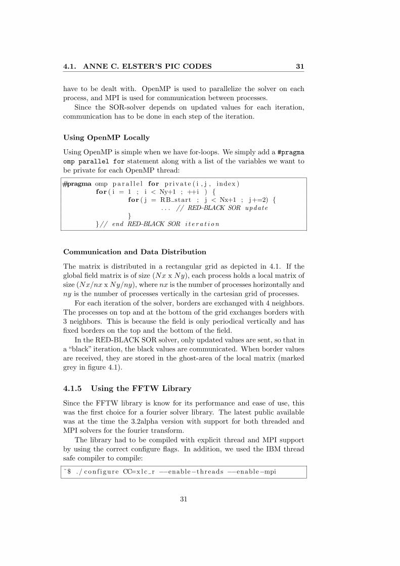
5.1 Efficiency for the FFTW solver on 64 CPUs with 1-5 thread(s)per CPU and 1-16 CPUs per MPI process. . . . . . . . . . . . 39
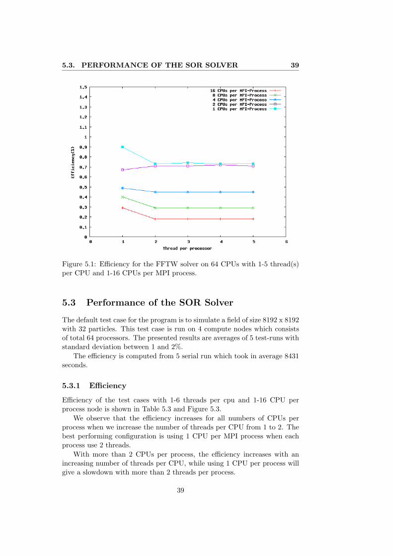
5.2 Wall-clock timings for the FFTW solver on 64 CPUs with 1-5thread(s) per CPU and 1-16 CPUs per MPI process. . . . . . 40
5.3 Efficiency for the SOR solver on 64 CPUs with 1-6 thread(s)per CPU and 1-16 CPUs per MPI process. . . . . . . . . . . . 41
5.4 Wall-clock timings for the SOR solver on 64 CPUs with 1-6thread(s) per CPU and 1-16 CPUs per MPI process. . . . . . 41
5.5 Data resides in the (orange)memory block, longest away fromCPU14 and CPU15. . . . . . . . . . . . . . . . . . . . . . . . 45
5.6 Timing results in seconds for original and optimized PIC code. 48
xi

xii

Chapter 1
Introduction
1.1 Motivation
Programming for parallel computing has been dominated by the MPI andOpenMP programming paradigms. Both of the paradims aims to providean interface for high performance, but their approach is somewhat different.
OpenMP is designed to shared memory systems, and has recently gainedpopularity because of its simple interface. With little effort, loops can easilybe parallelized with OpenMP, and much of the synchronization and datasharing is hidden from the user.
MPI is designed for distributed memory and is probably the best knownparadigm in parallel computing. Communication between processes is doneexplicitly, and a relatively large set of functions in the opens up for highperformance and tweaking which is not available in OpenMP. Even thoughit is designed for distributed memory systems, it runs just as good on sharedmemory systems.
Computer systems with both of OpenMP and MPI available opens upfor a hybrid programming style where both are used in the same application.The challenge on such systems is to find the optimal combination of the twoprogramming styles to achieve the best performance.
1.1.1 Thesis Goal
This thesis searches for the best configuration of OpenMP/MPI for optimalperformance. We will run a parallel simulation-application on a modernsupercomputer to measure the effects of different configurations of the mixedcode. After analyzing the performance of different configurations from ahardware point of view, we will propose a general model for estimatingoverhead in OpenMP loops.
We will parallelize a physics simulation to do large scale simulations asefficient as possible.
1

2 CHAPTER 1. INTRODUCTION
We will look at typical physics simulation codes to parallelize andoptimize them with OpenMP and MPI in a mixed mode. The goal of theparallelization is to make the code highly efficient for a parallel system andto make it as scalable as possible to do large-scale simulations as well asusing this parallelized application as a benchmark for our MPI/OpenMPtests.
1.2 Terminology
• PIC codes - Particle-In-Cell codes, a popular particle simulationtechnique for collision-less charged particles in electromagnetic fields.
• Processors - A physical processing unit. Several processors can beon one physical chip; dual-core consists of two processors on one chip.
• Processes - A program with private memory running on one or moreprocessors. A process can spawn several child processes or threads toutilize several processors.
• Threads - Threads are lightweight processes that can have bothshared and private memory. Processes consists often of two or morethreads.
• Nodes - One or more interconnected processors with shared memory.The interconnection does not consist of regular network, but of high-speed mediums as a fixed databus on a motherboard.
• FFT - Fast Fourier Transform. Used as a direct solver for partialdifferential equations.
• SOR - Successive Over Relaxation. Used to obtain an approximationof a solution for partial differential equations.
1.3 Thesis Outline
Chapter 1 contains this introduction.
Chapter 2 summarizes some of the important background theories andrelated work for this thesis. A short introduction to OpenMP and MPIis given, along with some de facto models for performance modeling.Classifications of supercomputer architectures are presented. The PICsimulation is also presented with some references to where more informationcan be found.
Chapter 3 describes the two PIC simulation codes we work on, andsome general background on how the general algorithm of PIC simulations
2

1.3. THESIS OUTLINE 3
are. Important steps of the algorithm is described and the SOR and fouriersolver are described. Both Jan Christian Meyer’s[3] and Anne C. Elster’ssimulation[1] are described, with some comments on initial performance andpotential performance improvements.
Chapter 4 contains a summary of the main changes done to thesimulation codes. The main changes are that two new solvers are introducedin Elster’s simulation code in addition to dealing with parallel issues of otherparts of the program.
Chapter 5 presents the performance results from our tests for both theMeyer and Elster versions of the PIC simulation. Different configurations ofthreads and processes on the SMP nodes are tested and the results arepresented. We also give a detailed analysis of the performance results.We also suggest a model for estimating the overhead when using OpenMPon more than one processor chip. The model is highly connected withthe hardware performance, more specifically memory latency and memorybandwidth.
Chapter 6 concludes the thesis and present some future works as acontinuation of this thesis.
3

4 CHAPTER 1. INTRODUCTION
4

Chapter 2
Background Theory
A dwarf on a giant’s shoulderssees farther of the two
Jacula Prudentum
This chapter gives a short introduction to the theory and technologyused in this project.
Some general introduction to performance modeling and Amdahl’s lawsare given in Section 2.1. The MPI and OpenMP API’s are introduced inSection 2.2 and 2.3. Programming models with these two API’s are describedin Section 2.4. Some common memory architectures are described in Section2.5 along with what programming models are suited for each of them. Ashort introduction to PIC-codes are given in Section 2.6. The math librariesused in this project are described in 2.8.
Previous and related works are described in Section 2.10, including thePIC codes this thesis is built upon and other existing PIC codes. An articleon hybrid parallel programming is summarized in 2.10.1.
2.1 Performance Modeling
The Laws of Amdahl are very general laws about performance and efficiencyof parallel applications. These laws are expressed by formulas for how wellparallel programs scale and how efficient they are compared to serial versionsof the same program, and are therefore often referred to when modelingperformance for MPI.
2.1.1 Amdahl’s Law
Amdahl’s Law[12] describes maximum expected improvement for an parallelsystem and is used to predict the maximum speedup of a parallel application.If a sequential program executes in a given time Tσ and the fraction r of the
5

6 CHAPTER 2. BACKGROUND THEORY
program is the part which can be parallelized, the maximum speedup S(p)for p processes is found by the formula
S(p) =Tσ
(1− r)Tσ + rTσ/p=
1(1− r) + r/p
(2.1)
If we differentiate S with respect to p and let p →∞, we get
S(p) → 11− r
(2.2)
from [12].This implies a theoretical limit of the speedup of a program when we
know the fraction of parallel code in the program.
2.1.2 Work and Overhead
Even if we parallelize the code perfectly, a parallel program will most likelyhave a worse speedup than predicted with the Amdahl’s Law. This is mainlydue to overhead from the parallelization. The sources of overhead are many,the most known are communication, creation of new processes and threads,extra computation and idle time.
The total work done by a serial program Wq is the runtime Tσ(n). Thework done by a parallel program Wπ is the sum of the work done by the pprocesses involved(2.3). Work includes idle time and all the extra overheadin the parallelization.
Wπ(n) =∑
Wq(n, p) = pTπ(n, p) (2.3)
from [12].Overhead TO is defined as the difference in work done by a parallel
implementation and a serial implementation of a given program. Theformula is given in equation 2.4. Overhead is mainly due to communicationand the cost of extra computation when parallelizing an application.
TO(n, p) = Wπ(n, p)−Wσ(n) = pTπ(n, p)− Tσ(n) (2.4)
from [12].
2.1.3 Efficiency
From the definitions of work and overhead we can derive the efficiency asthe work done by the serial application compared to the work done bythe parallel application. If we have no overhead at all(the ideal parallelapplication), the efficiency is 1. To achieve 100% efficiency, no same thingshould be computed on more than one node. The formula for efficiency isgiven in equation 2.5.
6

2.2. THE MESSAGE PASSING INTERFACE - MPI 7
E(n, p) =Tσ(n)
pTπ(n, p)=
W0(n)Wπ(n, p)
(2.5)
from [12].In theory, efficiency above 100% is impossible, but is in practice achieved
because of large cache sizes or the nature of datasets. Speedup above 100%for parallel applications is called superlinear speedup.
Communication
Communication is a source of overhead when parallelizing programs. Thetime to communicate a n-size message is roughly expressed with latency, Ts,and bandwidth, β, as
Tcomm = Ts + βn (2.6)
.
2.2 The Message Passing Interface - MPI
MPI[16] [24] is an industry standard for message passing communicationfor applications running on both shared and distributed memory systems.MPI allows the programmer to manage communication between processeson distributed memory systems. The MPI is an interface standard forwhat an MPI-implementation should provide of functions and what thesefunctions should do. There are several implementations of MPI andthe best known are probably MPICH and OpenMPI, both open sourceversion implementation. Most vendors of HPC resources also have theirown proprietary implementation of MPI with bindings for C, C++ andFortran. SCALI[4] is probably the best known Norwegian vendor of MPIimplementations.
The first MPI standard was presented at Supercomputing 19941 andfinalized soon thereafter. The first standard included a language independentspecification in addition to specifications for ANSI-C and Fortran-77.
About 128 functions are included in the MPI 1.2 specification. Thisinterface provides functions for the programmer to distribute data, synchronizeprocesses and create virtual topologies for communication between processes.
2.3 OpenMP
Shared memory architectures open up for efficient use of threads and sharedmemory programming models. The traditional way to take advantage
1November 1994
7
8 CHAPTER 2. BACKGROUND THEORY
of such architectures is to use threads in some way or other. POSIXthreads(pthreads) are most used in HPC programming, however threadmodels can quickly generate complex and unreadable code.
Recent advances in processor architectures with several cores on thesame chip has made shared memory programming models more interesting.Especially the introduction of dual-core processors for desktops the last twoyears2 has made this area of research interesting for other groups than theHPC communities.
OpenMP is an API that supports an easy-to-use shared memoryprogramming model. The easiness of inserting OpenMP directives into theparallel code has made this model popular compared to pthreads. Thismodel leaves most of the work of thread handling to the compiler and greatlyreduces the complexity of the code.
The directives for parallelization in OpenMP allows the user to decidewhat variables that should be shared and private in an easy way, in additionto what parts of the code that should be parallelized. The simplicity of usingOpenMP directives has made it a popular way of parallelizing applications.
2.4 Hybrid Programming Models
2.4.1 Classifications
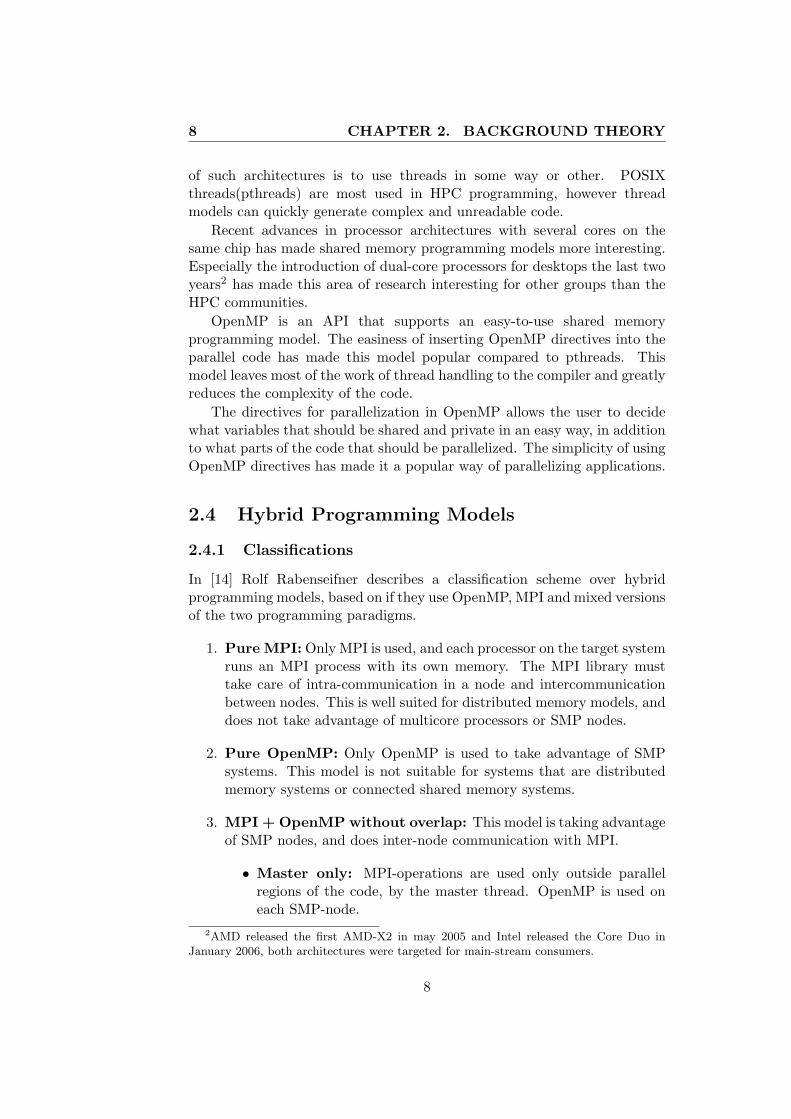
In [14] Rolf Rabenseifner describes a classification scheme over hybridprogramming models, based on if they use OpenMP, MPI and mixed versionsof the two programming paradigms.
1. Pure MPI: Only MPI is used, and each processor on the target systemruns an MPI process with its own memory. The MPI library musttake care of intra-communication in a node and intercommunicationbetween nodes. This is well suited for distributed memory models, anddoes not take advantage of multicore processors or SMP nodes.
2. Pure OpenMP: Only OpenMP is used to take advantage of SMPsystems. This model is not suitable for systems that are distributedmemory systems or connected shared memory systems.
3. MPI + OpenMP without overlap: This model is taking advantageof SMP nodes, and does inter-node communication with MPI.
• Master only: MPI-operations are used only outside parallelregions of the code, by the master thread. OpenMP is used oneach SMP-node.
2AMD released the first AMD-X2 in may 2005 and Intel released the Core Duo inJanuary 2006, both architectures were targeted for main-stream consumers.
8

2.5. SUPERCOMPUTER MEMORY MODELS 9
• Multiple: MPI-operations are used only outside parallel regions,but several cpus can participate in the communication. OpenMPis used on each SMP-node.
4. MPI + OpenMP with overlapping communication and computation:This is the optimal scheme for systems with connected SMP nodes.While one or more processors are handling communication, the otherprocessors are not left idle but does useful computation.
• Hybrid funneled: Only the master thread does MPI routines tohandle communication between SMP nodes. The other threadscan be used to do computation.
• Hybrid multiple: Several threads can call MPI-routines to handletheir own communication, or the communication is handled by agroup of threads.
2.5 Supercomputer Memory Models
Supercomputers come in many forms and are in this project roughlydivided into four groups: distributed memory systems, shared memorysystems, hybrid systems and grids. The respective groups are describedand illustrated with simplified figures below.
• Distributed memory systems(Fig. 2.1) share interconnection but haveprivate processor and memory. These systems are well suited formessage-passing libraries like MPI.
Figure 2.1: A distributed memory system.
• Shared memory systems(Fig. 2.2) are systems with more than oneprocessor where all processor’s share memory. These systems arewell suited for OpenMP, MPI, or mixed OpenMP-MPI programmingmodels. Each processor sees the memory as one large memory.
9

10 CHAPTER 2. BACKGROUND THEORY
Figure 2.2: A shared memory system.
• Hybrid Systems(Fig. 2.3) consist of two or more homogeneousinterconnected shared memory systems. These systems can runOpenMP and MPI on each node and use MPI for communicationbetween the nodes. This is the architecture of the Njord supercomputerat NTNU.
Figure 2.3: Connected shared memory nodes.
• Grids(Fig. 2.4) are heterogeneous systems where the only thing thecomponents must have in common is the software. OpenMP can bedeployed on the shared memory systems, and MPI can be used forcommunication between the nodes. Programming for grids can bemore challenging than programming for the other models because ofthe heterogeneous architecture.
10

2.6. PARTICLE-IN-CELL SIMULATIONS 11
Figure 2.4: A Heterogeneous network/grid of multicore shared memorysystems and single-core systems.
2.6 Particle-In-Cell Simulations
Particle-In-Cell(PIC) is a numerical approach to simulate how independentcharged particles interact with each other in a electric or magnetic field.Such simulations are used in various research areas such as astrophysics,plasma physics and semiconductor device physics[1]. The parallelizationof the PIC code done by Anne C. Elster has been used by Xerox in theirsimulations[5] to simulate how ink can be controlled by electric fields instandard ink-printers.
Depending on the size of these simulations, they can require morecomputation power than normal desktops offers and supercomputers thereforefrequently used to perform PIC simulations.
Simulation of PIC involves tracking the movement, speed and accelerationof particles in electric or magnetic fields. The particles are moving in amatrix of ’cells’ and contribute to the cells’ charge closest to them.
Solving the field is the operation to compute the charge-contributionfrom each particle to the field and update the field with correct values.Numerical methods for solving the field includes fourier transforms andapproximation methods like SOR.
For an extensive introduction to PIC codes, see [1]. For a lighterintroduction, see [3].
11

12 CHAPTER 2. BACKGROUND THEORY
2.7 PDE Solvers
By solvers we mean mathematical methods for solving a partial differentialequation(PDE). The PDE can, as in our case, describe physical fields withsome defined forces working on the field. The properties of the field defineswhat solvers can be used. Typical properties of the field includes periodic ornon-periodic borders, linearity and dimensionality. In general we can definetwo types of solvers for PDEs: direct and iterative.
2.7.1 Direct Solvers and the FFT
Direct solvers gives an exact solution for the PDE. Simple PDEs withoutcomplex borders or with periodic border conditions are typically solved withdirect solvers.
The Fourier Transform and the Discrete Fourier Transform, [1]
The Fourier Transform is a linear operator that transforms a function f(x)to a function F(w). The operator is described in detail in [1], but we willgive a short summary here.
If the function f(x) describes a physical process as a function of time,then H(ω) is said to represent its frequency-spectrum and ω are measuredin cycles per time unit x. In our case, the function f(x) describes distance,and the ω therefore describes angular frequency.
The fourier transform of a function f(x) is a function F (ω):
F (ω) =∫ ∞
x=−∞f(x)e−iωxdx (2.7)
and the inverse transform takes the function F (ω) back to f(x):
f(x) =12π
∫ ∞x=−∞
F (ω)eiωxdω (2.8)
It can be shown [1] that the second derivative of the original functionwould be the same as multiplying the transform with a constant,
d2f
d2x=
12π
∫ ∞x=−∞
(−ω2)F (ω)eiωxdω (2.9)
and therefore we can compute the second derivative of f(x) just as fast asa scaled fourier transform.
Since a computer cannot calculate continuous functions, The DiscreteFourier Transform (DFT) is constructed by discretizing the continuousfourier transform. Instead of integrating in a continuous space, we use
12
2.7. PDE SOLVERS 13
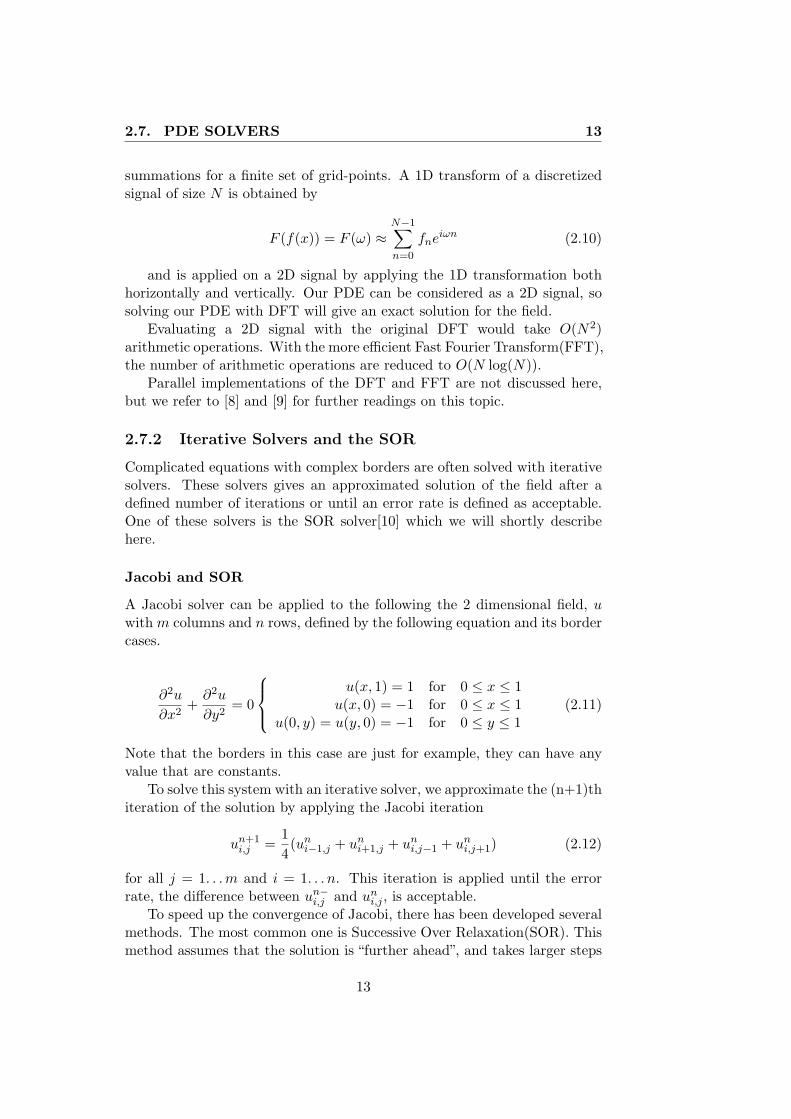
summations for a finite set of grid-points. A 1D transform of a discretizedsignal of size N is obtained by
F (f(x)) = F (ω) ≈N−1∑n=0
fneiωn (2.10)
and is applied on a 2D signal by applying the 1D transformation bothhorizontally and vertically. Our PDE can be considered as a 2D signal, sosolving our PDE with DFT will give an exact solution for the field.
Evaluating a 2D signal with the original DFT would take O(N2)arithmetic operations. With the more efficient Fast Fourier Transform(FFT),the number of arithmetic operations are reduced to O(N log(N)).
Parallel implementations of the DFT and FFT are not discussed here,but we refer to [8] and [9] for further readings on this topic.
2.7.2 Iterative Solvers and the SOR
Complicated equations with complex borders are often solved with iterativesolvers. These solvers gives an approximated solution of the field after adefined number of iterations or until an error rate is defined as acceptable.One of these solvers is the SOR solver[10] which we will shortly describehere.
Jacobi and SOR
A Jacobi solver can be applied to the following the 2 dimensional field, uwith m columns and n rows, defined by the following equation and its bordercases.
∂2u
∂x2+
∂2u
∂y2= 0
u(x, 1) = 1 for 0 ≤ x ≤ 1
u(x, 0) = −1 for 0 ≤ x ≤ 1u(0, y) = u(y, 0) = −1 for 0 ≤ y ≤ 1
(2.11)
Note that the borders in this case are just for example, they can have anyvalue that are constants.
To solve this system with an iterative solver, we approximate the (n+1)thiteration of the solution by applying the Jacobi iteration
un+1i,j =
14(un
i−1,j + uni+1,j + un
i,j−1 + uni,j+1) (2.12)
for all j = 1. . .m and i = 1. . .n. This iteration is applied until the errorrate, the difference between un−
i,j and uni,j , is acceptable.
To speed up the convergence of Jacobi, there has been developed severalmethods. The most common one is Successive Over Relaxation(SOR). Thismethod assumes that the solution is “further ahead”, and takes larger steps
13

14 CHAPTER 2. BACKGROUND THEORY
than Jacobi to converge faster. The SOR iteration is shown in Equatioin2.13, where ω is the degree of over-relaxation, usually between 1.7 and 1.85according to [1]. In addition, it also takes use of points already updated instep n + 1.
un+1i,j =
14(un+1
i−1,j + uni+1,j + un+1
i,j−1 + uni,j+1) + (1− ω)un
i,j (2.13)
Red-Black SOR
An optimization of SOR is the Red-Black SOR scheme. In the original SOR,each point is dependent of the previous updated point, making it hard toparallelize.
By dividing the points into red and black points formed like a chess-board, one can easily see that red points only depend on black points andvice versa. Therefore we can perform iterations where every other iterationcomputes the red and black points as shown in Figure 2.53.
In parallel implementations with n nodes of the SOR solver for fieldswith size N , each node typically has a matrix of size N
n in addition to ghostelements. Ghost elements are points received from neighbor nodes.
One SOR or Jacobi iteration takes O(N) operations per iteration if theequation is N big. How many iterations needed depends on the definedmaximum error rate.
For a further introduction to SOR solvers, see [10].
2.8 Math Libraries
When writing physics or math code, the use of ready libraries can ease thedevelopment and cut the development time drastically. Performance of manylibraries are often significantly faster than home made code, so if they areused we can get substantial performance gains. In this project we intendedto make use of the FFTW -libraries and the PETSc-libraries.
2.8.1 The “Fastest Fourier Transform in the West”
FFTW (”The Fastest Fourier Transform in the West”)[18], is a fairly newlibrary which performs the discrete fast fourier-transform(fft). It freelyavailable under the GPL license. It is written in C and is ported tomost POSIX-compliant systems, and increasingly more popular library.The performance of the library can often compete with machine-optimizedmath libraries according to [18]. The library consists of several discrete fft-implementations called codelets. With normal usage of the library, severalcodelets are tested to find the codelet that performs best on the specific
3The figure is copied with permission from [6].
14

2.8. MATH LIBRARIES 15
(i-1,j)
(i,j-1)
(i+1,j)
(i,j) (i,j+1)
Ghost elements
Ghost elements
Gh
ost
ele
men
ts
Gh
ost e
lem
ents
Figure 2.5: Red-black SOR with ghost elements. The red point (i, j) is onlydependent on black points.
processor-architecture. This way the best implementation is used for anyplatform. For updated information on features of FFTW, benchmarks anddocumentation, see [18].
2.8.2 Portable, Extensible Toolkit for Scientific Computation
PETSc,(Portable, Extensible Toolkit for Scientific Computation)[19], is aparallel library that contains sequential and parallel implementation forsolving partial differential equations. It uses MPI for it’s parallelization,and lets the users interact with distributed vectors and matrices in a uniformway. It is well documented and contains a lot of examples.
15
16 CHAPTER 2. BACKGROUND THEORY
2.9 Profilers
Profilers are programs which are made to give statistics about where timeis spent in an application. This is very useful for locating hot-spots andbottlenecks in an application.
2.9.1 Software profiling: gprof, prof
The most used way to make a profile of an application, is to compile withthe -g -p flags before it is run. This will reduce the performance of theapplication, but is only intended for use when optimizing or analyzingan application. Typical profilers are gpof, prof and tprof. For moreinformation on these, see AIX 5L Performance Tools Handbook, Chapter19 [11].
2.9.2 Hardware profiling: pmcount
To get a more hardware close profile of a program, program counterscan be used. These programs provides statistics about the hardwareperformance from hardware counters, resource utilization statistics andderived metrics. For parallel programs running on Power5/AIX systems,hpmcount is widespread and easy to use. It requires very little effort fromthe user and gives useful statistics about the hardware utilization.
2.10 Related Work
This section gives a brief introduction to the most central references onwhich this project is built.
2.10.1 Hybrid Parallel Programming on HPC Platforms
Rolf Rabenseifner has done a study[14] of performance of hybrid parallelprogramming patterns, as well as defining different categories for hybridmodels. In Hybrid Parallel Programming on HPC Platforms he evaluatesperformance on different architectures with the defined hybrid models. Thegoal is to find the hotspot-combination of MPI and OpenMP for performanceon each platform.
2.10.2 Parallelization Issues and Particle-In-Cell Codes
Anne C. Elster wrote her PhD dissertation[1] at Cornell University in 1994on Parallelization Issues and Particle-In-Cell Codes.
The dissertation is a comprehensive introduction to PIC simulation, anddescription of the field. Parallelization and memory issues are discussed indetail, along with a detailed description of the PIC algorithm.
16

2.10. RELATED WORK 17
The PIC-implementation from this dissertation uses a home-made FFTimplementation and has option to use pthreads for the parallel version.Neither MPI or OpenMP were used.
The work described in this report is highly related to Elster’s dissertation.
2.10.3 Emerging Technologies Project: Cluster Technologies.PIC codes: Eulerian data Partitioning
Jan Christian Meyer has written an other PIC implementation and a reporton the performance of it on two different architectures. The report waswritten in connection with the Emerging Technologies Project and is calledPIC Codes: Eulerian data partitioning [3].
The application uses MPI for parallelization, and a SOR solver.At the very beginning of this project, Meyer’s implementation was target
for optimization.
2.10.4 UCLA Parallel PIC Framework
UPIC(The UCLA Parallel PIC Framework) [7] is a framework for developmentof new particle simulation applications and is similar to the previous PICcodes described. It provides several solvers for different simulations and hasparallel support. It is written in Fortran95 and said to be “designed to hidethe complexity of parallel processing” and has error checks and debugginghelps included.
Since the authors of UPIC did not respond to our requests, we decidedto build our own framework for highly parallel PIC codes.
17

18 CHAPTER 2. BACKGROUND THEORY
18

Chapter 3
Particle-In-Cell Codes
All science is either physics orstamp collecting.
Ernest Rutherford
In this chapter we give an introduction to the general theory behind PICsimulations and introduction to two different implementations. In section3.1 the general PIC algorithm is described. Section 3.2 describes the PICcode implemented by Elster[1][2], while Section 3.3 describes the PIC codemade by Jan Christian Meyer.
3.1 General Theory
The general algorithm for a PIC simulation in [1] is given in Figure 3.1,and the components of the algorithm as in [1] is described in the followingsubsections.
1: Initialize(field, particles)2: while t < tmax do
3: Calculate particles contribution to field4: Solve the field5: Update particle speed6: Update particle position7: Write plot files
Figure 3.1: An general algorithm of a PIC simulation
3.1.1 The Field and the Particles
The physical field is represented as a discrete 2D array with Nx ∗ Nygridpoints. In the MPI-versions of PIC, each of the n MPI-processes is
19

20 CHAPTER 3. PARTICLE-IN-CELL CODES
computing a 1n share of the field.
The particles have 4 properties: charge, speed, location and weight.These values are described with double precision variables to give the neededamount of accuracy. Depending on the simulation, these properties have aninitial value or zero-values.
The size of the grid describing the field determines how high resolutionthe simulation will have.
3.1.2 A Particles Contribution to the Field
Since the particles position is represented with double precision numbers,and the field is represented by a non-continuous grid, the particles seldomare located exactly on one grid point. With high probability, the particle islocated as depicted in Figure 3.2 where the distance a and b varies. hy andhx are the grid-spaces in y and x direction.
(i,j)
(i+1,j) (i+1,j+1)
(i,j+1)
a
b hy
hx
(x0,y0)
Figure 3.2: A particle is located in a grid-cell of the field, contributing tothe charge of 4 grid-points.
Only the four grid-points surrounding a particle are updated, using thepseudo code in Listing 3.1 to update the grid-points. rhok is a scaling factorcomputed from the particles charge and the grid-spaces.
Listing 3.1: Updating the charge field from a particles position.f i e l d [ i , j ] += (hx − b) ∗ ( hy − a ) ∗ rho k ;f i e l d [ i , j +1] += b ∗ ( hy − a ) ∗ rho k ;f i e l d [ i +1, j ] += (hx − b) ∗ a ∗ rho k ;f i e l d [ i +1, j +1] += a ∗ b ∗ rho k ;
3.1.3 Solving the Field
The type of solver is chosen based on the properties of the field. Directsolvers like the fourier transform or iterative solvers like jacobi are typicalsolvers for the field, as described in Section 2.7.
20

3.2. ANNE C. ELSTER’S VERSION 21
3.1.4 Updating Speed and Position
To update a particles speed, we first need to find its acceleration. Theacceleration is computed from the charge of the particle, q, and the forcesfrom the field on the particle, E
F = q ∗ E (3.1)
where the field E can be decomposed into x and y direction, Ex and Ey.Speed is simply updated for x and y direction with
v = v0 +F
m(3.2)
where m is the mass of a particle.Updating a particles position is straight forward when we know its
speed and current position, simply add the timestep,5t, multiplied withthe updated speed, v, in both x and y direction.
Posx = Posx +5t ∗ vx (3.3)
Posy = Posy +5t ∗ vy (3.4)
3.2 Anne C. Elster’s Version
Anne C. Elster[1] implemented her PIC-application with an FFT solverfor 2 dimensions. The implementation uses a hand-optimized FFT solver.Elster used an FFT algorithm based on “Numerical Recipes”[9] that shehand-optimized at that time. At the time the program was built(1994)optimized math-libraries were not as widespread as it is today. The programis parallelized with Pthreads to run on a shared memory architecture.
3.2.1 Program Flow
This was the program flow of Elster’s original program.
1. Data describing the field and charges is read from input file tst.dat.
2. User types in size of grid to stdin.
3. Resources are allocated and speed and locations get initial values.Trace files are opened for a set of particles. Only particles are traced.Field charge is set to zero.
4. The field is updated with the charges of the particles.
5. Fourier solve of the field.
21
22 CHAPTER 3. PARTICLE-IN-CELL CODES
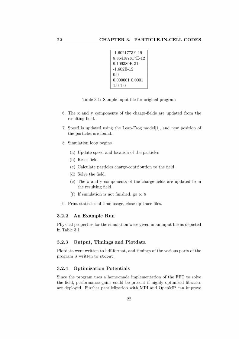
-1.6021773E-198.854187817E-129.109389E-31-1.602E-120.00.000001 0.00011.0 1.0
Table 3.1: Sample input file for original program
6. The x and y components of the charge-fields are updated from theresulting field.
7. Speed is updated using the Leap-Frog model[1], and new position ofthe particles are found.
8. Simulation loop begins
(a) Update speed and location of the particles
(b) Reset field
(c) Calculate particles charge-contribution to the field.
(d) Solve the field.
(e) The x and y components of the charge-fields are updated fromthe resulting field.
(f) If simulation is not finished, go to 8
9. Print statistics of time usage, close up trace files.
3.2.2 An Example Run
Physical properties for the simulation were given in an input file as depictedin Table 3.1
3.2.3 Output, Timings and Plotdata
Plotdata were written to hdf-format, and timings of the various parts of theprogram is written to stdout.
3.2.4 Optimization Potentials
Since the program uses a home-made implementation of the FFT to solvethe field, performance gains could be present if highly optimized librariesare deployed. Further parallelization with MPI and OpenMP can improve
22
3.3. JAN CHRISTIAN MEYER’S VERSION 23
the scalability for the program, as well as make it possible to run it on non-shared-memory systems. The program is only tested for small grids, i.e. Nxand Ny below 256.
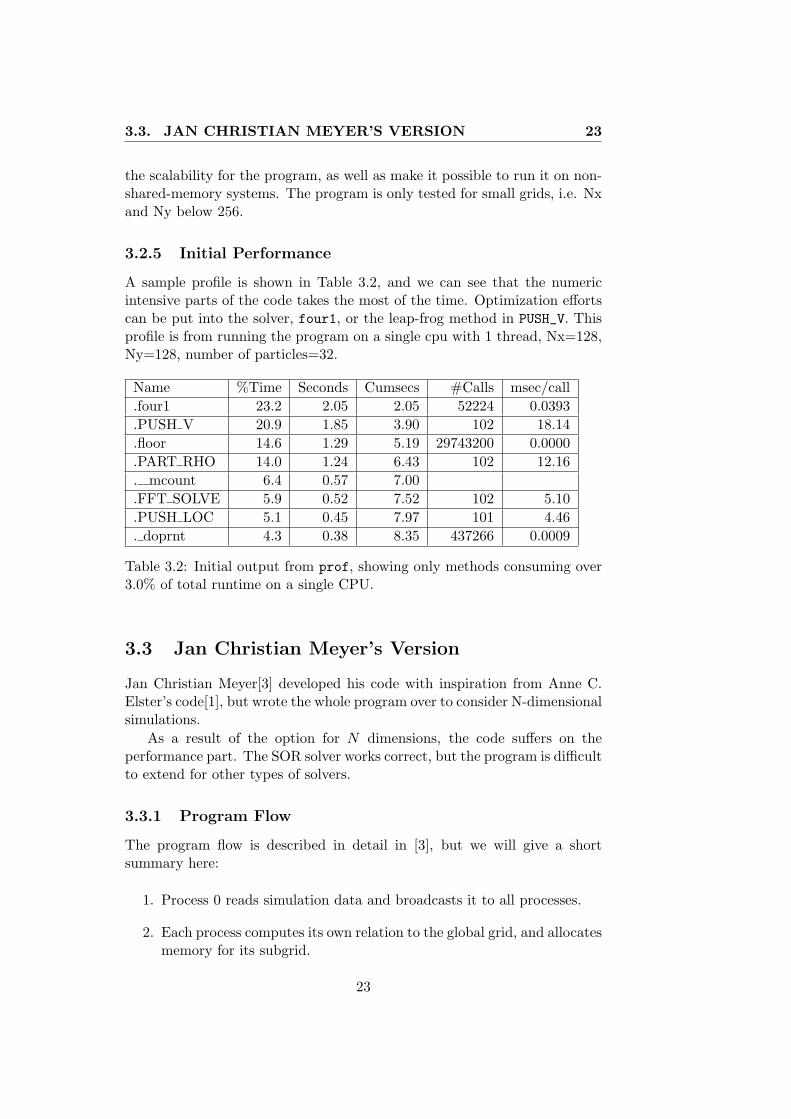
3.2.5 Initial Performance
A sample profile is shown in Table 3.2, and we can see that the numericintensive parts of the code takes the most of the time. Optimization effortscan be put into the solver, four1, or the leap-frog method in PUSH_V. Thisprofile is from running the program on a single cpu with 1 thread, Nx=128,Ny=128, number of particles=32.
Name %Time Seconds Cumsecs #Calls msec/call.four1 23.2 2.05 2.05 52224 0.0393.PUSH V 20.9 1.85 3.90 102 18.14.floor 14.6 1.29 5.19 29743200 0.0000.PART RHO 14.0 1.24 6.43 102 12.16. mcount 6.4 0.57 7.00.FFT SOLVE 5.9 0.52 7.52 102 5.10.PUSH LOC 5.1 0.45 7.97 101 4.46. doprnt 4.3 0.38 8.35 437266 0.0009
Table 3.2: Initial output from prof, showing only methods consuming over3.0% of total runtime on a single CPU.
3.3 Jan Christian Meyer’s Version
Jan Christian Meyer[3] developed his code with inspiration from Anne C.Elster’s code[1], but wrote the whole program over to consider N-dimensionalsimulations.
As a result of the option for N dimensions, the code suffers on theperformance part. The SOR solver works correct, but the program is difficultto extend for other types of solvers.
3.3.1 Program Flow
The program flow is described in detail in [3], but we will give a shortsummary here:
1. Process 0 reads simulation data and broadcasts it to all processes.
2. Each process computes its own relation to the global grid, and allocatesmemory for its subgrid.
23
24 CHAPTER 3. PARTICLE-IN-CELL CODES
3. Process 0 reads particle number and the initial position and speed foreach particle. The particles are sent to its respective positions andprocesses in the global grid.
4. Simulation loop begins:
(a) All processes opens plot files for timings and particle data.
(b) The charge is distributed from the particles in each subgrid of thefield.
(c) Each process sends the boundaries of their subgrid to its respectiveneighbour processes.
(d) The field is solved both locally and globally, and field strength isobtained for each subgrid.
(e) All subgrids interpolates the electric field strength at the particlescurrent position.
(f) Speed and position of particles are update. Particles are sentbetween processes if they cross subgrid borders.
(g) If the simulation is not finished, go to 4.
5. All resources are freed.
3.3.2 An Example Run
This section will describe what is needed for execution of the program andoutput produced by the program.
Configuration and Inputs
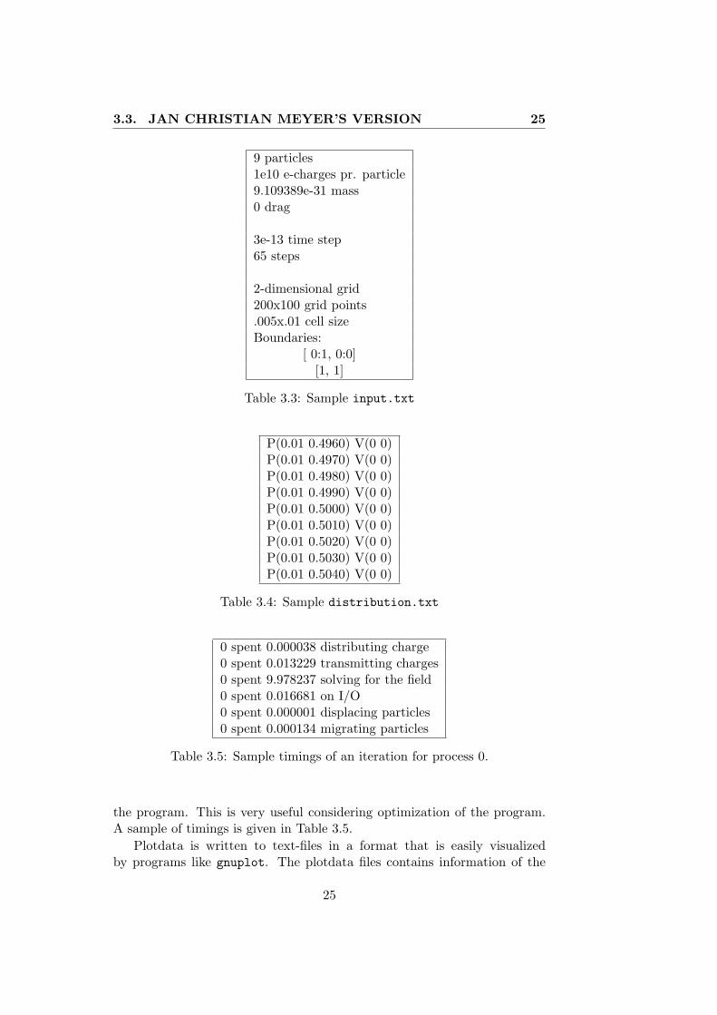
The program is compiled and linked into one executable file, simulation.The executable takes two text-files as arguments, input.txt and distribution.txt.input.txt contains information about the field and the configuration of thesolver as given in Table 3.3.
distribution.txt contains information about the particles in thesimulation. The number of entries should be the same as specified ininput.txt. Initial speed and location is given as in Table 3.4.
3.3.3 Output - stderr, Timings and Plotdata
The program has mainly three output types: stderr, information abouttimings and plotdata. stderr is used only to print the status of whatiteration is finished.
The timings contains information for each step and for each processinvolved in the program on how long time is spent in the various regions of
24
3.3. JAN CHRISTIAN MEYER’S VERSION 25
9 particles1e10 e-charges pr. particle9.109389e-31 mass0 drag
3e-13 time step65 steps
2-dimensional grid200x100 grid points.005x.01 cell sizeBoundaries:
[ 0:1, 0:0][1, 1]
Table 3.3: Sample input.txt
P(0.01 0.4960) V(0 0)P(0.01 0.4970) V(0 0)P(0.01 0.4980) V(0 0)P(0.01 0.4990) V(0 0)P(0.01 0.5000) V(0 0)P(0.01 0.5010) V(0 0)P(0.01 0.5020) V(0 0)P(0.01 0.5030) V(0 0)P(0.01 0.5040) V(0 0)
Table 3.4: Sample distribution.txt
0 spent 0.000038 distributing charge0 spent 0.013229 transmitting charges0 spent 9.978237 solving for the field0 spent 0.016681 on I/O0 spent 0.000001 displacing particles0 spent 0.000134 migrating particles
Table 3.5: Sample timings of an iteration for process 0.
the program. This is very useful considering optimization of the program.A sample of timings is given in Table 3.5.
Plotdata is written to text-files in a format that is easily visualizedby programs like gnuplot. The plotdata files contains information of the
25

26 CHAPTER 3. PARTICLE-IN-CELL CODES
potential of the field, an example of visualization is given in figure 3.3.
Figure 3.3: Sample visualization of potential in the field. Plotted in gnuplotfrom plotdata, step 4 of the simulation.
3.3.4 Optimization Potentials
The code was not written with optimal performance in mind [3], so thepotential for improvements in runtime for the original code was indeedpresent. Since a simple and naive SOR-implementation is used, performancegains could be achieved by using a solver from a math library, e.g. anoptimized fft-solver or an optimized SOR-solver.
3.3.5 Initial Performance
This subsection gives some numbers and statistics on performance of theoriginal program.
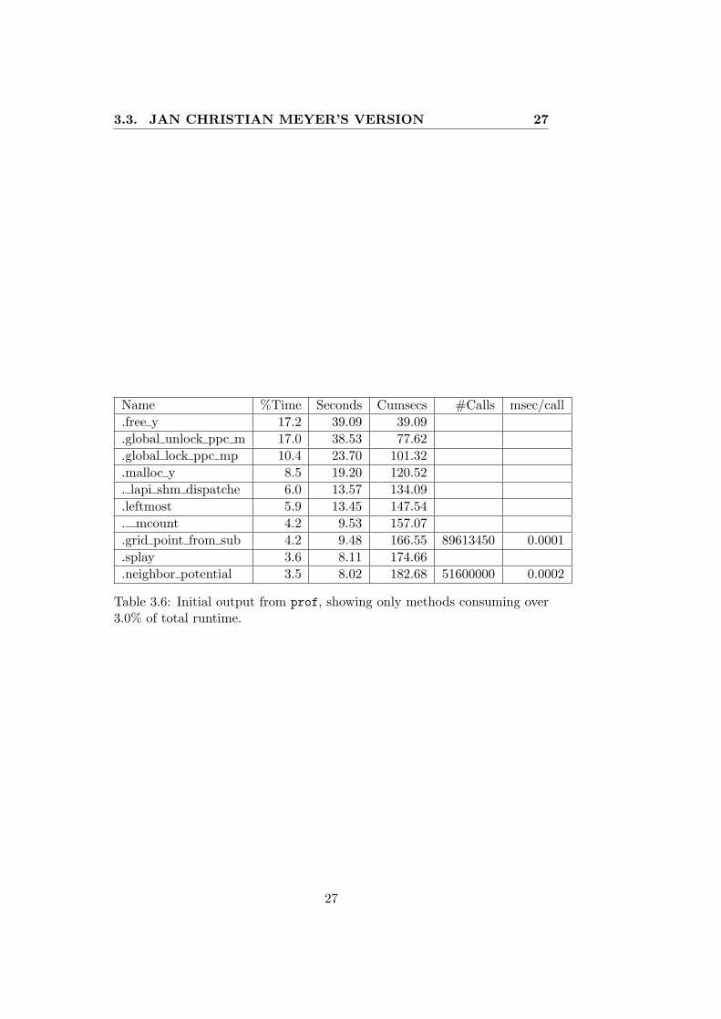
Timings and Profiling
The output from the profiling program gprof is shown in Table 3.6. As wecan see, the program uses a lot of time allocating and freeing memory. Whilememory management uses about 53% of the time(the top 4 functions), theneighbor_potential() function uses only 3.5% of the time.
26
3.3. JAN CHRISTIAN MEYER’S VERSION 27
Name %Time Seconds Cumsecs #Calls msec/call.free y 17.2 39.09 39.09.global unlock ppc m 17.0 38.53 77.62.global lock ppc mp 10.4 23.70 101.32.malloc y 8.5 19.20 120.52. lapi shm dispatche 6.0 13.57 134.09.leftmost 5.9 13.45 147.54. mcount 4.2 9.53 157.07.grid point from sub 4.2 9.48 166.55 89613450 0.0001.splay 3.6 8.11 174.66.neighbor potential 3.5 8.02 182.68 51600000 0.0002
Table 3.6: Initial output from prof, showing only methods consuming over3.0% of total runtime.
27

28 CHAPTER 3. PARTICLE-IN-CELL CODES
28

Chapter 4
Optimizing PIC Codes
In this chapter, we will describe the changes made to existing codes. Section4.1 describes the changes and extensions made to Anne C. Elster’s PICapplication[1]. Section 4.2 describes the modifications done to Jan ChristianMeyer’s PIC application[3]. The main focus is on the codes developed byAnne C. Elster.
4.1 Anne C. Elster’s PIC codes
Elster’s PIC code from [1] was written back in 1994 for the KSR(KendallSquare Research) shared memory system. The single-threaded versioncompiled cleanly after some minor changes, and a more extensive Makefilewas created before any features were added.
4.1.1 Changes to Existing Code
The existing code implements the fourier transform to solve the field, so anatural extension was to take use of a fourier library to improve the runtimeof the existing code with minimal changes. This is described in 4.1.5.
To perform tests with hybrid MPI/OpenMP we implemented a parallelSOR solver as described in Section 4.1.4.
An unsuccessful attempt to deploy the PETSc library is described inSection 4.1.6.
The virtual process-topologies used for data distribution of the matricesand communication are different for the FFTW- and SOR-solver.
Parallel Pseudo Algorithm
This algorithm describes both the FFTW and the SOR version of thesimulation, changes made in this thesis involve only step 5b and 5d in thepseudo code.
29
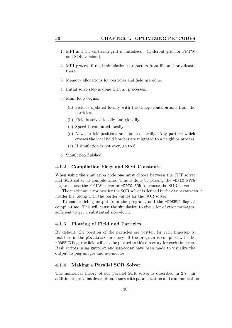
30 CHAPTER 4. OPTIMIZING PIC CODES
1. MPI and the cartesian grid is initialized. (Different grid for FFTWand SOR version.)
2. MPI process 0 reads simulation parameters from file and broadcaststhese.
3. Memory allocations for particles and field are done.
4. Initial solve step is done with all processes.
5. Main loop begins.
(a) Field is updated locally with the charge-contributions from theparticles.
(b) Field is solved locally and globally.
(c) Speed is computed locally.
(d) New particle-positions are updated locally. Any particle whichcrosses the local field borders are migrated to a neighbor process.
(e) If simulation is not over, go to 5.
6. Simulation finished
4.1.2 Compilation Flags and SOR Constants
When using the simulation code one must choose between the FFT solverand SOR solver at compile-time. This is done by passing the -DPIC_FFTWflag to choose the FFTW solver or -DPIC_SOR to choose the SOR solver.
The maximum error rate for the SOR solver is defined in the declarations.hheader file, along with the border values for the SOR solver.
To enable debug output from the program, add the -DDEBUG flag atcompile-time. This will cause the simulation to give a lot of error messages,sufficient to get a substantial slow-down.
4.1.3 Plotting of Field and Particles
By default, the position of the particles are written for each timestep totext-files in the plotdata/ directory. If the program is compiled with the-DDEBUG flag, the field will also be plotted to this directory for each timestep.Bash scripts using gnuplot and mencoder have been made to visualize theoutput to png-images and avi-movies.
4.1.4 Making a Parallel SOR Solver
The numerical theory of our parallel SOR solver is described in 2.7. Inaddition to previous description, issues with parallelization and communication
30
4.1. ANNE C. ELSTER’S PIC CODES 31
have to be dealt with. OpenMP is used to parallelize the solver on eachprocess, and MPI is used for communication between processes.
Since the SOR-solver depends on updated values for each iteration,communication has to be done in each step of the iteration.
Using OpenMP Locally
Using OpenMP is simple when we have for-loops. We simply add a #pragmaomp parallel for statement along with a list of the variables we want tobe private for each OpenMP thread:
#pragma omp p a r a l l e l for pr i va t e ( i , j , index )for ( i = 1 ; i < Ny+1 ; ++i ) {
for ( j = RB start ; j < Nx+1 ; j+=2) {. . . // RED−BLACK SOR update
}}// end RED−BLACK SOR i t e r a t i o n
Communication and Data Distribution
The matrix is distributed in a rectangular grid as depicted in 4.1. If theglobal field matrix is of size (Nx x Ny), each process holds a local matrix ofsize (Nx/nx x Ny/ny), where nx is the number of processes horizontally andny is the number of processes vertically in the cartesian grid of processes.
For each iteration of the solver, borders are exchanged with 4 neighbors.The processes on top and at the bottom of the grid exchanges borders with3 neighbors. This is because the field is only periodical vertically and hasfixed borders on the top and the bottom of the field.
In the RED-BLACK SOR solver, only updated values are sent, so that ina “black” iteration, the black values are communicated. When border valuesare received, they are stored in the ghost-area of the local matrix (markedgrey in figure 4.1).
4.1.5 Using the FFTW Library
Since the FFTW library is know for its performance and ease of use, thiswas the first choice for a fourier solver library. The latest public availablewas at the time the 3.2alpha version with support for both threaded andMPI solvers for the fourier transform.
The library had to be compiled with explicit thread and MPI supportby using the correct configure flags. In addition, we used the IBM threadsafe compiler to compile:
˜$ . / c on f i gu r e CC=x l c r −−enable−threads −−enable−mpi
31

32 CHAPTER 4. OPTIMIZING PIC CODES
Neighbor process
Neighbor process
Neig
hb
or
pro
cess
Neig
hb
or
pro
cess
m
Process m
Figure 4.1: Data distribution and communication pattern in parallelRED/BLACK-SOR solver.
Using Threads Locally
The FFTW-library lives up to its reputation as an easy-to-use library, evenwhen using the threaded version. The only code changes from the serial orMPI-version is that we add two lines of code before we set up the solver:
f f tw p lan w i th nth r eads ( num threads ) ;
This configures the solver to make the solver use num_threads threadsfor each MPI process.
MPI-setup, Communication and Data Distribution
The FFTW-library is responsible for communication during the solver step,so this is hidden for the user. Communication patterns also depends whichfft algorithm the FFTW-library chooses to use. The FFTW-library providesthe following code to set up a MPI-parallel solver:
f f tw mp i i n i t ( ) ;a l l o c l o c a l = f f tw mp i l o c a l s i z e 2 d ( . . . ) ;data = f f tw ma l l o c ( a l l o c l o c a l ∗ s izeof ( f f tw complex ) ) ;s o l v e r f o rwa rd = f f tw mpi p lan d f t 2d ( . . . , FFTWFORWARD ) ;so lver backward = f f tw mpi p lan d f t 2d ( . . . , FFTWBACKWARD ) ;
To execute the solver, we simply state:
32

4.1. ANNE C. ELSTER’S PIC CODES 33
f f tw ex e cu t e d f t ( so lve r f o rward , data , data ) ;// . . . opera te on the transformed data here . . .f f tw ex e cu t e d f t ( so lver backward , data , data ) ;
The data distribution has to be the way FFTW defines if the program isto run correctly. The data distribution is very simple, and allows us to makea flat cartesian grid of size 1xN , where N is the total number of processesin the simulation. The global field matrix is divided among the processes asdepicted in figure 4.2. If the global field matrix is of size (Nx x Ny), thelocal matrix would be (Nx/N x Ny), where N is the number of processes.
1 2 3 ... N
Figure 4.2: Data distribution for N processes in the MPI-parallel FFTWsolver.
4.1.6 Using the PETSc Library
The PETSc library is a well known library for solving PDEs on parallelmachines, but is also known to be a bit difficult to use. This was alsoour experience, and after about a week of trying to make it work with ourexisting code, we gave up. The main problem was that we could not mapthe local data we already had in our code into the PETSc funtcions and getthe data back into our structures again after solving the PDE.
4.1.7 Migration of Particles Between MPI Processes
When a particle cross the local field border, it is sent to a neighbor processin the respective direction. This is done by the MPI_Isend() procedure fromthe sending process. All processes checks for incoming particles by using theMPI_Probe() function with MPI_ANY_SOURCE as source parameter. This is
33

34 CHAPTER 4. OPTIMIZING PIC CODES
done to ensure that we receive particles from any of our neighbor processes.If the result from the probe function indicates an incoming message, theparticle and its properties are received and stored in the local particle arrays.This is repeated until there are no more incoming particles. If a process hassent particles, the MPI_Waitall() function is used to ensure that all sentparticles are transmitted successfully.
4.1.8 SOR Trace
To check if the program produces correct output, the plottings for 19particles can be observed in Figure 4.1.8. The particles close to the zero-charged lower border, and move up to the 0.00001V charged upper border.
The particles are attracted to the positive boundary, while they are alsorepelled by each other, so that the trace leaves a typical SOR “fan”.
Figure 4.3: Traces of particles from a simulation using the SOR solver for16 particles in a 0.2 x 0.2 field with 64x64 gridpoints.
4.2 Jan Christian Meyer
The code from [3] was working up to a point, but had a memoryleakage as we describe in 4.2.1. As the report[3] describes, this code wasleft unoptimized and had a great potential of performance improvement.Performance improvements and obstacles are described in 4.2.2. Because ofthe complexity of the code, OpenMP or threads where not deployed in thisPIC code.
34

4.2. JAN CHRISTIAN MEYER 35
4.2.1 Initial Bugfixes
In [3] Section 7.2, the code is described to sometimes saturate and crash thesystem. After some reading and debugging, the error was discovered to bea memory leak in one of the frequently used functions.
As memory leakages most, the bug was first found after late hours ofdebugging and wrapping of free() and malloc() functions. The memoryleakage was due to the subgrid_neighbor_coordinates variable in themethod neighbor_potential(). Memory was allocated for the variablefor each time the method was called, but never freed again. This causedthe program to exceed its memory limits and therefore got killed by thebatch-system.
4.2.2 General Performance Improvements
Since this code was written to intentionally be a PIC simulator for Ndimensions, the datatypes and solver functions had to be as general aspossible regarding dimensions. This has made the code harder to read andalso harder to optimize without major changes to the existing code.
Another issue is that memory is frequently allocated and freed throughoutthe program, and memory management takes a lot of time as shown fromthe initial profile in Table 3.6. By allocating and freeing memory in theinnermost loops, potential performance gains might have been lost. Insteadof being cpu-bound, the code is memory bound. The most important changewas therefore simply to allocate most of the memory only at the start of theprogram, and free it again at the end of the program.
In the innermost loop in the function neighbor_potential(), some ifstatements and switch-case statements were re-written to avoid branch-mispredictions.
35

36 CHAPTER 4. OPTIMIZING PIC CODES
36

Chapter 5
Results and Discussion
Observations always involvetheory.
Edwin Hubble
This chapter contains presentation of the performance results of the PICsimulations and discussion of these results. The emphasis is on Anne C.Elster’s PIC codes.
Section 5.1 contains a brief description of the computer and processorsused for the tests.
Section 5.2 contains the performance results for the FFTW solver withdifferent ratios of MPI processes and OpenMP threads. Section 5.3 containsperformance results for our parallel SOR solver with different ratios of MPIprocesses and OpenMP threads.
Section 5.4 explains the super-linear speedup in the results from ourSOR solver. Section 5.5 describes the effect of the SMT feature in our tests.Analysis about hidden overhead in OpenMP loops and a model to estimatethe communication in loops is described in Section 5.6.
In the end of the chapter we look at the results from optimizing Jan C.Meyer’s PIC code in Section 5.7 and 5.8.
5.1 Hardware specifications
The specific processor we have been testing on is the Power5+ chip with 2processor-cores with 64KB private level 1 data-cache, 1.9MB private level 2cache and 36MB shared level 3 cache[20] as given in Table 5.1.
The system is a IBM p575 system with all in all 56 shared memory nodesof 8 dual cores and 32 GB Memory each. The interconnect between thenodes is IBM’s proprietary “Federation” interconnect which provides highbandwidth and low latency. More information on the specific system can befound in IBM’s whitepaper on p575 [20].
37

38 CHAPTER 5. RESULTS AND DISCUSSION
Frequency(Ghz) 1.9L2 Latency(cycles) 12L3 Latency(cycles) 80Memory Latency(cycles) 220L1 Size 64KbL2 Size 1.9MbL3 Size 36Mb
Table 5.1: Power5+ CPU specifications, quoted from [20], [21] and [22].
5.2 Performance of the FFTW solver
In this section we present the performance results from the FFTW-solver inAnne C. Elster’s PIC code.
The test case is a field of size 8192 x 8192 with 32 particles. The programis run on 4 compute nodes which gives a total of 64 processors. The presentedresults are averages of 5 test-runs with standard deviation between 1 and2%.
5.2.1 Efficiency
The efficiency is computed from 5 serial runs which took in average 4207seconds. The efficiency for the FFTW solver is presented in Table 5.2 andFigure 5.1.
Threads/CPUCPUs/Processes
1 2 4 8 16
1 0.90 0.67 0.49 0.40 0.292 0.73 0.71 0.45 0.29 0.183 0.74 0.71 0.45 0.29 0.184 0.73 0.72 0.45 0.29 0.185 0.73 0.71 0.45 0.29 0.18
Table 5.2: Efficiency for the FFTW solver on 64 CPUs with 1-5 thread(s)per CPU and 1-16 CPUs per MPI process.
We observe that the most efficient configuration is 1 MPI process perCPU where each process uses only 1 thread. Only when we use 2 CPUs perprocess we get a slight speedup from increasing the number of threads.
An efficiency of 0.9 indicates that the FFTW-solver scales well on 64processors. The difference in efficiency from the best to the worst performingconfiguration of the FFTW solver is 72%.
38
5.3. PERFORMANCE OF THE SOR SOLVER 39
Figure 5.1: Efficiency for the FFTW solver on 64 CPUs with 1-5 thread(s)per CPU and 1-16 CPUs per MPI process.
5.3 Performance of the SOR Solver
The default test case for the program is to simulate a field of size 8192 x 8192with 32 particles. This test case is run on 4 compute nodes which consistsof total 64 processors. The presented results are averages of 5 test-runs withstandard deviation between 1 and 2%.
The efficiency is computed from 5 serial run which took in average 8431seconds.
5.3.1 Efficiency
Efficiency of the test cases with 1-6 threads per cpu and 1-16 CPU perprocess node is shown in Table 5.3 and Figure 5.3.
We observe that the efficiency increases for all numbers of CPUs perprocess when we increase the number of threads per CPU from 1 to 2. Thebest performing configuration is using 1 CPU per MPI process when eachprocess use 2 threads.
With more than 2 CPUs per process, the efficiency increases with anincreasing number of threads per CPU, while using 1 CPU per process willgive a slowdown with more than 2 threads per process.
39
40 CHAPTER 5. RESULTS AND DISCUSSION
0
50
100
150
200
250
300
350
400
0 1 2 3 4 5 6
Wall-t
ime(
s)
Thread per processor
16 CPUs per MPI-Process
�������
3
3 3 3 3 3
8 CPUs per MPI-Process
""""""
+
+ + + +
+4 CPUs per MPI-Process
((((((22 2 2 2
2
2 CPUs per MPI-Process
× × × × ×
×1 CPUs per MPI-Process
((((((
44 4 4 4
4
Figure 5.2: Wall-clock timings for the FFTW solver on 64 CPUs with 1-5thread(s) per CPU and 1-16 CPUs per MPI process.
Threads/CPUCPU/Process
1 2 4 8 16
1 1.22 0.78 0.79 0.65 0.552 1.59 1.49 1.28 1.10 0.903 1.46 1.43 1.49 1.19 1.054 1.36 1.41 1.44 1.12 0.995 1.24 1.44 1.47 1.22 1.096 1.17 1.45 1.40 1.24 1.10
Table 5.3: Efficiency for the SOR solver on 64 CPUs with 1-6 thread(s) perCPU and 1-16 CPUs per MPI process.
From Table 5.3 and Figure 5.3 we see that our SOR solver scales wellfor 64 processors with the right configuration. The super-linear speedup isexplained in later sections.
The difference in between the best and worst configuration for the SORsolver is 104%.
5.4 Super-linear speedup
super-linear speedup is defined as speedup greater than than the number ofprocessor used, thus we get an efficiency greater than 1.
40

5.4. SUPER-LINEAR SPEEDUP 41
0
0.2
0.4
0.6
0.8
1
1.2
1.4
1.6
1.8
2
2.2
2.4
0 1 2 3 4 5 6 7
Effi
cien
cy
Thread per processor
16 CPUs per MPI-Process
"""""���
��hhhhh(((((
3
3
33
3 3
3
8 CPUs per MPI-Process
�����(((((hhhhh(((
((
+
++
++ +
+4 CPUs per MPI-Process
#####�����hhhhh hhhhh
2
2
2 2 22
2
2 CPUs per MPI-Process
%%%%%%hhhhh
×
× × × × ×
×1 CPUs per MPI-Process
"""""`̀ `̀ `hhhhh`̀ `̀ `hhhhh4
44
44 4
4
Figure 5.3: Efficiency for the SOR solver on 64 CPUs with 1-6 thread(s) perCPU and 1-16 CPUs per MPI process.
0
50
100
150
200
250
300
350
400
0 1 2 3 4 5 6 7
Wall-t
ime(
s)
Thread per processor
16 CPUs per MPI-Process
@@@@@`̀ `̀ ` hhhhh
3
33 3
3 3
3
8 CPUs per MPI-Process
lllllhhhhh hhhhh
+
+ + + + +
+4 CPUs per MPI-Process
QQQQQhhhhh
2
22 2 2 2
2
2 CPUs per MPI-Process
ccccc
×
× × × × ×
×1 CPUs per MPI-Process
XXXXX(((((4
4 4 4 44
4
Figure 5.4: Wall-clock timings for the SOR solver on 64 CPUs with 1-6thread(s) per CPU and 1-16 CPUs per MPI process.
There can be various reasons for super-linear speedup, one of them is the
41
42 CHAPTER 5. RESULTS AND DISCUSSION
data set size compared to cache size. Cache is the fastest type of memory ina computer, and is considerably faster than regular memory. In the followingsubsection we consider our test case for the SOR solver and its super-linearspeedup.
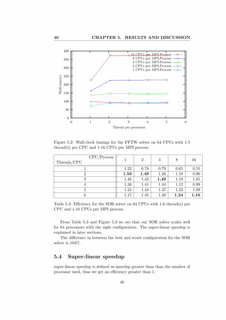
5.4.1 Cache hit rate
Our test case is 8192 x 8192 big. The solver function needs about
8192 ∗ 8192 ∗ sizeof(byte)Bytes = 512MBytes (5.1)
of space in memory. When divided on 4 nodes with 8 dual core chips, thedata set on each chip is
512MBytes
4Nodes ∗ 8Dualcores= 16MBytes/Dualcore (5.2)
which fits in level 3 cache of the power5+ dualcore chip. From Table 5.1 weknow that L3 cache has a latency of 80 cycles compared to the 220 clockcycles of the main memory. Any application that are I/O intensive wouldthus gain from having the entire dataset in L3 cache instead of main memory.
In addition to a speedup from the dataset fitting into level 3 cache, thereare also potential gains in exploiting the size of level 1 cache for datasetswith certain dimensions.
A matrix of 1048 x N double-precision floating point elements will havematrix row of 1048. A double-precision number takes 8 bytes, and therefore3 rows of the matrix takes
1048 ∗ 8 ∗ 3Bytes = 24576KB (5.3)
which fits in the level 1 cache, enabling the SOR algorithm to update atleast one full row of the matrix without cache misses. When doing the SORalgorithm we use values from 3 rows(upper, lower and current row) of thematrix to update an element. In our test with global matrix size of 8192 x8192 on 64 processors, each processor holds a 1024 x 1024 matrix, which willgive super-linear speedup compared to the serial run where 3 matrix rowsdoesn’t fit in level 1 cache. The maximum row size to fit in a 64KB level 1cache is
64 ∗ 10243 ∗ 8
= 2730 (5.4)
. The implemented SOR algorithm will therefore theoretically favourmatrices with up to about 2730 columns will therefore have an super-linearspeedup on the Power5+ processor.
42
5.5. SIMULTANEOUS MULTITHREADING 43
5.5 Simultaneous Multithreading
The Power5+ architecture provides a technology called Simultaneous Multi-threading (SMT), which allows for fast thread and process switches andbetter utilization of the instruction pipeline.
By increasing the number of threads to a number greater than processors,several threads are waiting at the same time, and the idle time of one threadcan be used by another thread to compute. This means that algorithms thatcauses frequent pipeline stalls or are frequently waiting for memory loads tocomplete, could get a speedup.
The SMT technology allows for the thread-switching to happen withoutthe need of flushing the instruction pipeline, and we can efficiently use moreof the cycles spent idling when fewer threads are used. Idling is a result ofa thread not filling the pipeline with instructions, or only filling it partially.
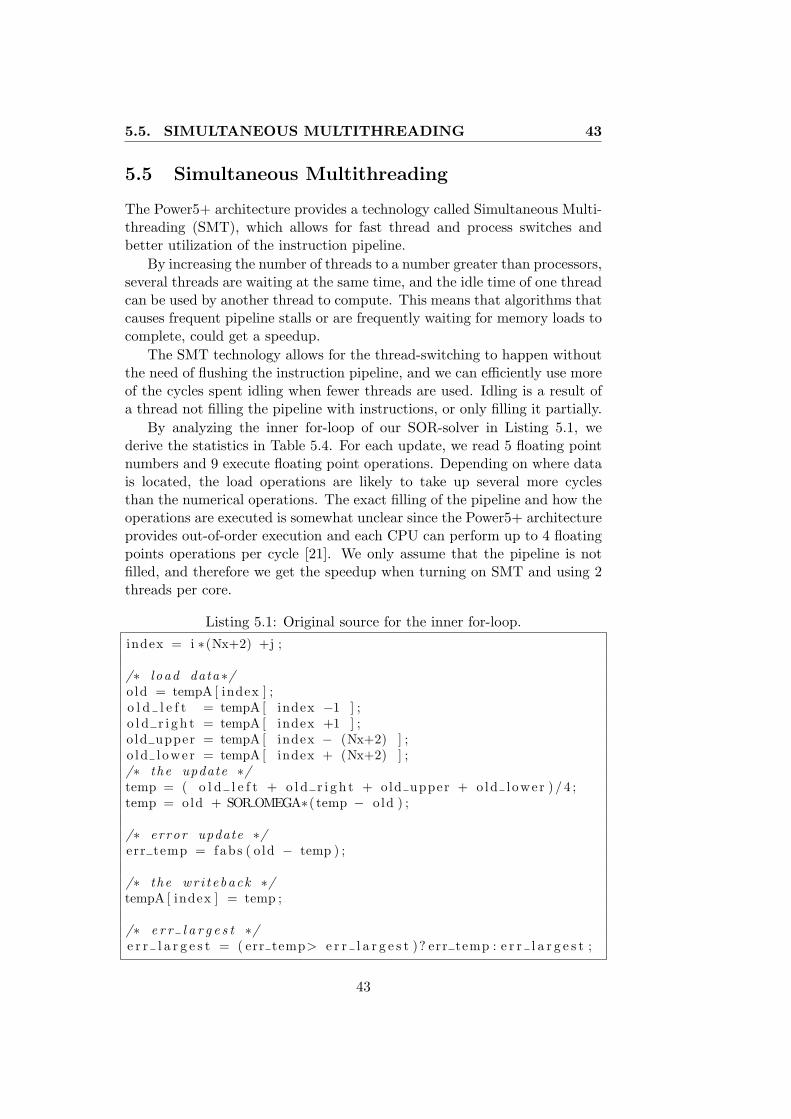
By analyzing the inner for-loop of our SOR-solver in Listing 5.1, wederive the statistics in Table 5.4. For each update, we read 5 floating pointnumbers and 9 execute floating point operations. Depending on where datais located, the load operations are likely to take up several more cyclesthan the numerical operations. The exact filling of the pipeline and how theoperations are executed is somewhat unclear since the Power5+ architectureprovides out-of-order execution and each CPU can perform up to 4 floatingpoints operations per cycle [21]. We only assume that the pipeline is notfilled, and therefore we get the speedup when turning on SMT and using 2threads per core.
Listing 5.1: Original source for the inner for-loop.index = i ∗(Nx+2) +j ;
/∗ l oad data ∗/o ld = tempA [ index ] ;o l d l e f t = tempA [ index −1 ] ;o l d r i g h t = tempA [ index +1 ] ;o ld upper = tempA [ index − (Nx+2) ] ;o ld l ower = tempA [ index + (Nx+2) ] ;/∗ the update ∗/temp = ( o l d l e f t + o l d r i g h t + old upper + o ld lower ) / 4 ;temp = old + SOR OMEGA∗( temp − o ld ) ;
/∗ error update ∗/err temp = fabs ( o ld − temp ) ;
/∗ the wr i t e back ∗/tempA [ index ] = temp ;
/∗ e r r l a r g e s t ∗/e r r l a r g e s t = ( err temp> e r r l a r g e s t )? err temp : e r r l a r g e s t ;
43

44 CHAPTER 5. RESULTS AND DISCUSSION
Operation type Name Count Cycles/operationLoad lfd and lfdux 5 1/12/80/220(L1/L2/L3/RAM)Store stfdux 1 1/12/80/220(L1/L2/L3/RAM)
Total load/store 6Add fadd 3 6p
Subtract fsub 2 6p
Multiply fmul 1 6p
Multiply-add fmad 1 6p
Absolute value fabs 1 6p
Compare fcmpu 1 6p
Total numerical 9 54p
Total 15
Table 5.4: Operation counts for the inner for-loop of the SOR solver.Numbers denoted p are pipelined operations.
From both Figure 5.1 and 5.3 we see that the SOR solver performsbest with 2 threads per MPI process and 1 MPI process per core. For theFFTW solver, 2 threads gives a slow-down. The SOR algorithm has an O(n)analytical runtime while the FFTW has an O(nlog(n)) analytical runtime,and therefore also has roughly log(n) times numerical operations per load-operation than the SOR. We have measured this with the pmcount commandTODO: read latest results from frigg
5.6 Communication Overhead in OpenMP
The overhead related to OpenMP is mistakenly often only related to theoverhead related to spawning and destruction of threads in addition to somesynchronization. The overhead from communication between the threads onthe different processors is often forgotten or neglected because it is hiddenfrom the programmer.
A node on Njord consists of 8 dual core processors and 32 GB of memory.The layout is illustrated in Figure 5.5, reproduced and simplified from [20].
When running tests with a 8192 x 8192 matrix on 4 nodes, we must usea minimum of
8129 ∗ 8129 ∗ sizeof(double)Bytes
4nodes= 128Mb (5.5)
data on each node.How the data is exactly located on each node is of not known, but assume
that the matrix is located as depicted in Figure5.5, where the orange memoryblock contains the matrix data. Now, when our SOR algorithm uses 16OpenMP threads, all the processors will access the memory block in all
44

5.6. COMMUNICATION OVERHEAD IN OPENMP 45
iterations of the solver. For the processors to retrieve this memory, theprocessors longest away from the data might have to idle several cycles toget the data to be processed. This will happen even if the data is notdistributed as in Figure5.5, because of the nature OpenMP.
CPU0CPU1
CPU2CPU3
Memory
Memory
Memory
Memory
Memory
Memory
Memory
Memory
Memory
Memory
Memory
Memory
Memory
Memory
Memory
Memory
CPU4CPU5
CPU6CPU7
CPU8CPU9
CPU10CPU11
CPU12CPU13
CPU14CPU15
Figure 5.5: Data resides in the (orange)memory block, longest away fromCPU14 and CPU15.
In the pure MPI test-runs, the data is located in a memory bank close tothe processor, so the idle time when waiting for memory is avoided becauseof the close proximity to the memory[20]. With small data sets, the MPI-processes achieve greater performance because all of the data resides in thelevel 3 cache, and maximum memory latency is reduced from 220 to 80 clockcycles when accessing data.
With several threads sharing data, a significant source of overhead isintroduced with communication of the data between the processors, and theoverhead increases by the number of threads:
• 1 CPU per process.
– 1 thread. There is no overhead in communication betweenthreads.
– 2 threads. Shared L1, L2 and L3 cache minimizes the overhead.SMT is used so that there is no cost of context-switches of threads.
– More than 2 threads. Overhead from thread-switching.
45
46 CHAPTER 5. RESULTS AND DISCUSSION
• 2 CPU per process. Overhead from communication. Since the 2CPUs are located on the same chip, communication between threadson the cores is done via the L3 cache. Threads on the same corecommunicates via the L1 and L2 cache.
• 4 - 16 PCU per process In addition to the mentioned overhead,there is also overhead from communication between the dualcore chips.The communication is no longer done via cache, but via main memoryor a fast databus.
The total overhead, Ot, for an OpenMP loop on processors executed bya number of threads can be expressed as
Ot = Tcomm + Tthreads (5.6)
Where Tcomm is the time spent in communication and Tthreads is theoverhead from spawning, destroying and switching between active threads.
For a for-loop in OpenMP, a loop of i iterations is divided into chunksizes of c, so that the number of messages sent is
i
c(5.7)
and the size, s, of the messages are
s = c ∗ sizeof(datatype) (5.8)
.The cost of communication of c bytes is known to be
Tcomm = Ts + βs (5.9)
where Ts is the latency of the respective cache level or memory wherethe data is located and β is the bandwidth between the processors.
Summarizing these formulas, we get a general expression for overhead ofcommunication in an OpenMP for-loop,
Tcomm =i
c(Ts + β ∗ c ∗ sizeof(datatype)) (5.10)
.There are three variables in this equation we should look into to provide
a better understanding of the estimate, the bandwidth β, cache-latency Ts
and chunk size c.
• β can be approximately measured with MPI-benchmarks limited to 1and only 1 SMP node. Repeatedly broadcasts or all-to-all benchmarkswith long messages can give an estimate of the intra-node-bandwidth.The bandwidth could well be related to how many processors that
46

5.6. COMMUNICATION OVERHEAD IN OPENMP 47
share communication bus, so this variable could be decreasing as thenumber of processors increases.
• Ts can be found with the same method as β, only with NULL-sizemessages. Depending on how many processors that participate in thecomputation, the length of the databus and how many processors usingthe databus at the same time will influence the latency. As moreprocessors participate in the for-loop, it is likely that we end up witha decreasing average latency.
• The chunk size c can be specified statically with the OpenMP keywordschedule(static, chunk size). This is however not recommended,since a normal programmer seldom knows the optimal chunk size. Bynot specifying the chunk size, it is set to be decided in runtime andtherefore difficult to know. Finding the optimal chunk size can bedone empirically by comparing different chunk sizes to the defaultschedule(runtime).
5.6.1 Fixed Chunk Size
As mentioned in feedback1 of a presentation of early results from this thesis[23], the overhead of communication could be reduced by setting a staticchunk size to a size so that each thread in the OpenMP loop only receivesdata once. Then the number of messages is limited to the number of threadsinvolved.
However, further testing with this theory indicates that we get little orno speedup in our SOR algorithm with this strategy. This could be becauseof border-exchanges of chunks during the calculation, or that the latency,Ts, is less significant than the bandwidth, β, in Equation 5.10.
5.6.2 Thread Affinity
In feedback2 from [23], it was mentioned that thread-affinity could influencethe performance results. If a thread migrates to an other CPU for somereason, this migration takes extra time and must be included in the overheadcalculation.
To test if this was a significant source of overhead, we used thebindprocess() function-call to bind the OpenMP threads to a given CPU.However, this did not give any notable performance improvements. Sincethe bindprocess() function did not give any improvement, it might be thatthreads already are bound to a CPU in IBM’s OpenMP-implementation, orthat threads did not migrate before we used the bindprocess() call.
1Comments from Thorvald Natvig2Comments from Jørn Amundsen
47
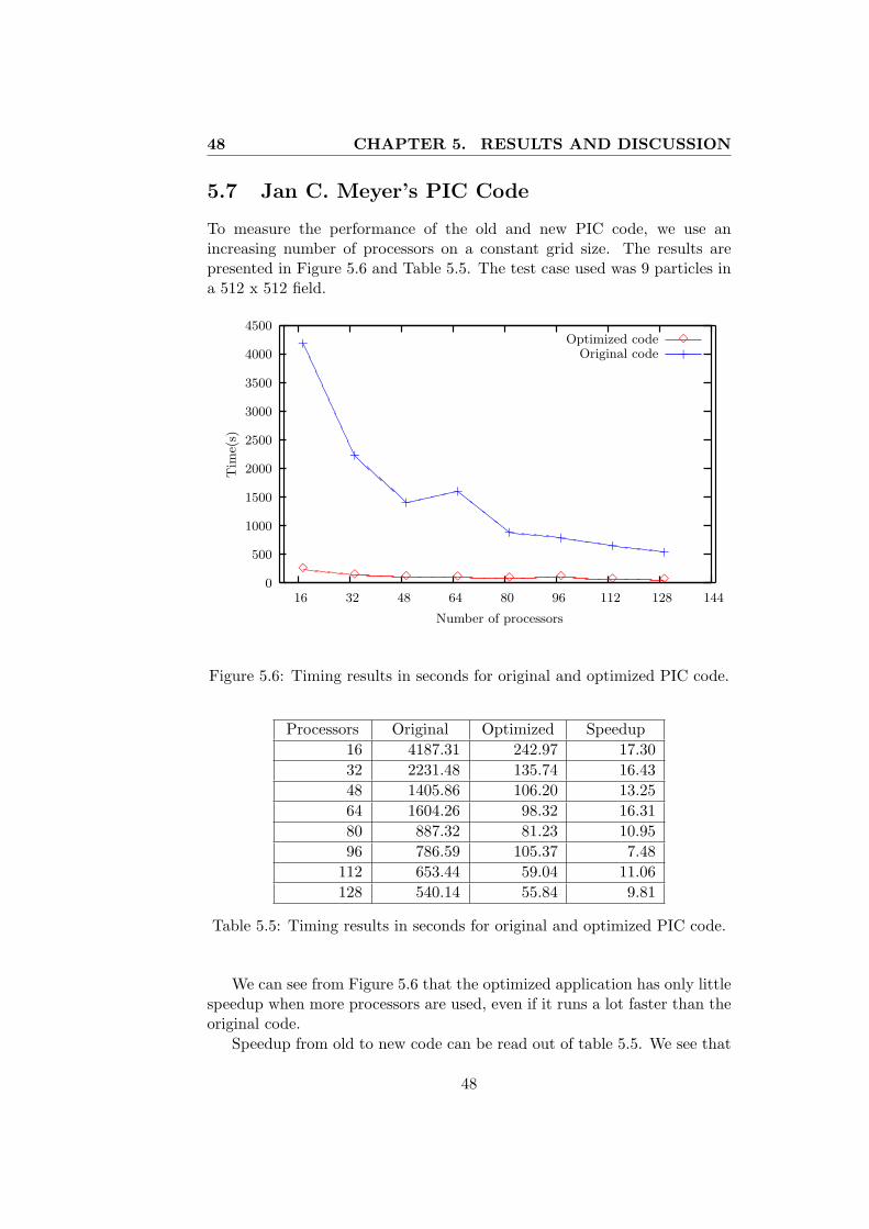
48 CHAPTER 5. RESULTS AND DISCUSSION
5.7 Jan C. Meyer’s PIC Code
To measure the performance of the old and new PIC code, we use anincreasing number of processors on a constant grid size. The results arepresented in Figure 5.6 and Table 5.5. The test case used was 9 particles ina 512 x 512 field.
0
500
1000
1500
2000
2500
3000
3500
4000
4500
16 32 48 64 80 96 112 128 144
Tim
e(s)
Number of processors
Optimized code
hhhh33 3 3 3 3 3 3
3
Original codeAAAAAAAA@@@@
cccchhhhhhhhhhhh
+
+
++
+ ++ +
+
Figure 5.6: Timing results in seconds for original and optimized PIC code.
Processors Original Optimized Speedup16 4187.31 242.97 17.3032 2231.48 135.74 16.4348 1405.86 106.20 13.2564 1604.26 98.32 16.3180 887.32 81.23 10.9596 786.59 105.37 7.48
112 653.44 59.04 11.06128 540.14 55.84 9.81
Table 5.5: Timing results in seconds for original and optimized PIC code.
We can see from Figure 5.6 that the optimized application has only littlespeedup when more processors are used, even if it runs a lot faster than theoriginal code.
Speedup from old to new code can be read out of table 5.5. We see that
48

5.8. EFFECTS OF CORRECT MEMORY ALLOCATION INJAN C. MEYER’S PIC CODE 49
the new code has a substantial speedup compared to the old code.
5.8 Effects of Correct Memory Allocation in JanC. Meyer’s PIC Code
The only optimization we did to Jan C. Meyer’s code was to handle memoryallocations better. However, the application was from about 10 to 17 timesfaster after this optimization. This demonstrates only that even smalloptimizations can lead to significant performance improvements.
49

50 CHAPTER 5. RESULTS AND DISCUSSION
50

Chapter 6
Conclusion
Men love to wonder, and that isthe seed of science.
Ralph Waldo Emerson
In this thesis we parallelized a PIC simulation to study hybrid OpenMP/MPIcode and evaluated the performance of different configurations of these twoprogramming paradigms.
6.1 Contribution
In this thesis we have
1. Proposed a general model for estimating overhead in for-loops inOpenMP.
2. Did a study of OpenMP and MPI in combination to find that MPIprovides the best performance of the two programming styles.
3. Parallelized an existing Particle-In-Cell simulation with OpenMP andMPI. From the results we see that the resulting application is highlyscalable and efficient.
4. Optimized an existing Particle-In-Cell simulation to handle memory-allocations better.
Hybrid OpenMP and MPI Codes
To parallelize the PIC codes we have used both OpenMP and MPI toexplore the possibilities of maximum performance. MPI was used globally toexchange border-values and particles while OpenMP was used to parallelizecompute-intensive for-loops. While OpenMP is the easiest way to parallelize
51

52 CHAPTER 6. CONCLUSION
loops, our results showed that overhead from communication between theprocessors makes it a low-performing API compared to MPI where data iscommunicated explicitly.
We suggested a general expression to model the overhead of communicationin OpenMP loops based on number of loop-iterations, chunksize, latency andbandwidth.
Parallelization and Optimization of PIC Codes
We converted a Particle-In-Cell code using Pthreads and optimized it withMPI and OpenMP. The results has shown that the codes are highly scalableand efficient. In addition to the original FFT algorithm, there is now optionsto use either the FFTW solver or our parallel SOR-solver depending on theborder conditions. The parallelization includes a cartesian division of thefield where all processors holds a small part of the field. Particles migratebetween processors efficiently using MPI_Isend() when particles move fromone local field to another.
We also improved the way memory was allocated and freed in Jan C.Meyer’s PIC code, in addition to some other minor changes. This has leadto a 10-17 times speedup compared to the original application.
6.2 Future work
• During the project we requested for some other PIC-codes from [7],but we have still not had the chance to try this code. A natural futurework is to compare the performance of such codes to our own, and seewhat has been done different in other versions.
• From a physics point of view, the codes could be extended to includemore complex physical properties like different charged particles andmore complex border boundaries.
• Further analysis on how many clock cycles are used per SOR updatewould be interesting to find out. However, such an analysis mightrequire a simulation of the power5 architecture to obtain exactnumbers.
• Further investigations and other programs using OpenMP should beexplored to find accurate methods to estimate the overhead of usingOpenMP.
• Compare the FFTW library to FFT-implementation in the IBM mathlibrary, PESSL. There might be some speedup from FFTW to thePESSL library since PESSL is optimized for the power architecture.
52

6.2. FUTURE WORK 53
• The SOR solver could be optimized even more. To avoid reading andwriting conflicts between the threads, we could split the field matrixinto one“black”matrix and one“red”matrix. This way, all the threadsneeds only to read one of the matrices, and enable all threads to havea local copy of the read-matrix without any synchronization during ared/black SOR iteration.
• Load balancing is a topic we have not been looking at in this thesis.If there are many particles in a simulation, we might end up with oneMPI-process with all the particles, and also all the computation relatedto the particles. A direct future work would be to look at how suchload-balancing have been done in other simulations, and implement itin Anne C. Elster’s PIC codes.
53
Bibliography
[1] Anne C. Elster, “Parallelization Issues and Particle-In-Cell Codes”, 1994,Cornell University, USA.
[2] Anne C. Elster, “Software Test-bed for Large Parallel Solvers”, 1999, IterativeMethods in Scientific Computation IV, 245-260.
[3] Jan C. Meyer, “Emerging Technologies Project: Cluster Technologies. PICcodes: Eulerian data partitioning. ,” 2004, Norwegian University of Scienceand Technology, Norway.
[4] SCALI higher performance computing, http://www.scali.com/
[5] Ted Retzlaff and John G. Shaw , “Simulation of Multi-component ChargedParticle Systems”, 2002, Wilson Center for Research and Techology , XeroxCorporation, USA.
[6] Thorvald Natvig, “Automatic Optimization of MPI Applications”, January2006, Norwegian University of Science and Technology, Norway.
[7] Viktor K. Decyk and Charles D. Norton, “UCLA Parallel PIC Framework,”,January 2006, University of Los Angeles, USA.
[8] James W. Cooley and John W. Tukey, ”An algorithm for the machinecalculation of complex Fourier series,” Math. Comput. 19, 297-301, 1965.
[9] William H. Press, Saul A. Teukolsky, William T. Vetterling, Brian P. Flannery,Numerical Recipes in C, The Art of Scientific Computing, CambridgeUniversity Press, 1992, USA.
[10] David M. Young, Iterative Solution of Large Linear Systems, 461-481, 2003,Dover Publications, USA.
[11] Budi Darmawan, Charles Kamers, Hennie Pienaar and Janet Shiu, AIX5L Performance Tools Handbook, August 2003, IBM International TechnicalSupport Organization, http://ibm.com/redbooks .
[12] Peter S. Pacheco, Parallel Programming with MPI, 1997, Morgan KaufmannPublishers, San Fransisco, USA.
[13] Timothy G. Mattson, Beverly A. Sanders, Berna L. Massingill, Patterns forParallel Programming, Addison Wesley Professional , September 2004, Boston,MA, USA.
[14] Rolf Rabenseifner, “Hybrid Parallel Programming on HPC Platforms,”EWOMP’03, September 22-26 2003, Aachen, Germany.
[15] The Unix System – UNIX 03 - http://www.unix.org/unix03.html
[16] The Message Passing Interface(MPI) Standard - http://www-unix.mcs.anl.gov/mpi/ and http://www.mpi-forum.org
54
[17] OpenMP: Simple, Portable, Scalable SMP Programming -http://www.openmp.org/
[18] “The Fastest Fourier Transform in The West”, FFTW - http://fftw.org/
[19] “Portable, Extensible Toolkit for Scientific Computation”, PETSc -http://www-unix.mcs.anl.gov/petsc/petsc-as/
[20] Harry M. Mathis, Frederick Bothwell, Jacob Thomas, “IBMSystem p5 575 8-core 2.2 GHz, 16-core 1.9 GHz Ultra-dense,Modular Cluster Nodes for High Performance Computing”,February 2006, IBM Systems and Technology Group http://www-03.ibm.com/systems/p/hardware/whitepapers/575 hpc.html
[21] B. Sinharoy, R. N. Kalla, J.M. Tendler, R.J. Eickmeyer J.B. Joyner,“POWER5 System Microarchitecture”, July 2005, IBM Systems andTechnology Group.
[22] TOP500 Supercomputing Sites, http://www.top500.org
[23] Presentation of this thesis to the NTNU HPC Group, May 25th, NTNU,Norway.
[24] Anne C. Elster and David L. Presberg, “Setting Standards For ParallelComputing: The High Performance Fortran and Message Passing InterfaceEfforts ”, May 1993, Theory Center SMART NODE Newsletter, Vol. 5, No.3. http://www.idi.ntnu.no/ elster
55

56

Appendix A
Description of Source Code
This chapter describes the functionality of each file in Anne C. Elster’sparallelized PIC code.
A.1 Dependencies
To compile and run the simulation you will need the following softwareinstalled:
• POSIX compliant system. Linux and AIX 5.3 have been tested.
• MPI is a need for running the shared-memory version of the program.
• FFTW with support for MPI, this means version 3.2 or later. MPIand thread support must be compiled in explicitly with -enable-mpi-enable-threads.
• OpenMP must be supported by the compiler to use the OpenMP versionof the SOR solver.
• Support for affinity should be provided by the system by some ofthe files in the /usr/include/sys directory. In AIX this is thesys/processor.h file.
• gnuplot is convenient for visualizing the output from the simulation.Most of the output is built to interact easily with gnuplot.
A.2 Compilation
Depending on the system you are on, you might want to change the Makefile.The variables FFTW_DIR and MPI_HOME should point to their respectivedirectories. Compiler, CC, and compiler flags should probably also beadjusted by needs and preferences.
57
A.3 Source Code
A.3.1 declarations.h
• Pre-defined constants used throughout the program.
• SOR constants for Dirichlet borders, maximum error rate and maximumnumber of iterations the SOR solver should do.
• Global variables.
• Function declarations for all functions in the simulation.
A.3.2 mymacros.h
Contains basic function-macros made by Anne C. Elster.
A.3.3 common.c
Contains some functions that does not fit in the simulation or solver category.Debug functions and plotting functions.
A.3.4 solvers.c
Contains a wrapper function, generic_solve(), and all solvers. generic_solvechooses what solver to use from compiler flags (either -DPIC_FFTW or -DPIC_SOR). Old solvers and solvers under work can be chosen by modifyinggeneric_solve().
A.3.5 psim.c
Contains the main function of the program and all functions that calculatesparticles contribution and speed.
• main contains the main-loop of the simulation.
• part_rho calculates each particles contribution to the field.
• uniform_grid_init initializes each particles initial speed and position.
• periodic_field_grid calculates the field at each node in x and ydirection.
• push_v calculates acceleration and updates speed of the particles.
• push_loc updates a particles location based on it speed and currentlocation.
In addition, there are some old trace-functions in this source file we leftuntouched. The original trace functions of the particles uses the hdf format.
58