Large Scale Character Classification

Thesis submitted in partial fulfillment

of the requirements for the degree of

Master of Science (by Research)

in

Computer Science

by

Neeba N.V

200650016

neeba@research.iiit.ac.in

http://research.iiit.ac.in/~neeba

International Institute of Information Technology

Hyderabad, India

August 2010

ii

INTERNATIONAL INSTITUTE OF INFORMATION TECHNOLOGY

Hyderabad, India

CERTIFICATE

It is certified that the work contained in this thesis, titled Large Scale Character Classi-

fication by Neeba N.V, has been carried out under my supervision and is not submitted

elsewhere for a degree.

Date Advisor: Dr. C. V. Jawahar

iv

Copyright c© Neeba N.V, 2008

All Rights Reserved

vi

To my Loving parents.

viii

O Lord, May I accept gracefully, what I can not change.

O Lord, May I have the will and effort to change what I can change.

O Lord, May I have the wisdom to understand, what I can change, and What I can

not Change.

x

Acknowledgements

I am deeply indebted to my advisor Dr. C. V. Jawahar for his kindness, dedication,

encouragement, motivation and also for his inspiring guidance and supervision throughout

my thesis work. I am also greatly indebted to Dr. P. J. Narayanan (PJN) for his concern,

encouragement and advise. My sincere thanks also forwarded to Dr. Anoop M. Namboodiri

for his critical comments on my conference papers.

I would also like to thank document understanding research groups at Centre for Vi-

sual Information Technology (CVIT), who had made great contribution by sharing ideas,

comments and materials. My dearest thanks goes to Anand Kumar, Million Meshesha,

Jyotirmoy, Rasagna, and Jinesh for their valuable suggestions and kindness to help me in

any way possible. A special thanks goes to my friend Ilayraja, who was my project partner

for the work ”Efficient Implementation of SVM for Large Class Problems”. I extend my

thanks to my friends Lini, Satya, Pooja and Uma for their support during my MS.

Last, but not the least, the almighty, my parents, my relatives and all those from CVIT

who had at some or the other point in time helped me with their invaluable suggestions

and feedback, and my research center, Center for Visual Information Technology (CVIT),

for funding my MS by research in IIIT Hyderabad.

Abstract

Large scale pattern classification systems are necessary in many real life problems like

object recognition, bio-informatics, character recognition, biometrics and data-mining. This

thesis focuses on pattern classification issues associated with character recognition, with

special emphasis on Malayalam. We propose an architecture for the character classification,

and proves the utility of the the proposed method by validating on a large dataset. The

challenges we address in this work includes: (i) Classification in presence of large number of

classes (ii) Efficient implementation of effective large scale classification (iii) Simultaneous

performance analysis and learning in large data sets (of Millions of examples).

Throughout this work, we use examples of characters (or symbols) extracted from real-

life Malayalam document images. Developing annotated data set at the symbol level from a

coarse (say word-level) annotated data is addressed first with the help of a dynamic program-

ming based algorithm. Algorithm is then generalized to handle the popular degradations

in the form of cuts, merges and other artifacts. As a byproduct, this algorithms allows

to quantitatively estimate the quality of the books, documents and words. The dynamic

programming based algorithm aligns the text (in UNICODE) with images (in Pixels). This

helps in developing a large data set which could help in conducting large scale character

classification experiments.

We then conduct an empirical study of classifiers and feature combination to explore their

suitability to the problem of character classification. The scope of this study include (a)

applicability of a spectrum of popular classifiers and features (b)scalability of classifiers with

the increase in number of classes (c) sensitivity of features to degradation (d) generalization

across fonts and (e) applicability across scripts. It may be noted that all these aspects

are important to solve practical character classification problems. Our empirical studies

provide convincing evidences to support the utility of SVM (multiple pair-wise) classifiers

for solving the problem.

However, a direct use of multiple SVM classifiers has certain disadvantages: (i) since

there are nC2 pairwise classifiers, storage and computational complexity of the final classifier

becomes high for many practical applications. (ii) they directly provide a class label and fail

to provide an estimate of the posterior probability. We address these issues by efficiently

designing a Decision Directed Acyclic Graph (DDAG) classifier and using the appropriate

feature space. We also propose efficient methods to minimize the storage complexity of

support vectors for the classification purpose. We also extend our algebraic simplification

method for simplifying hierarchical classifier solutions.We use SVM pair-wise classifiers with

DDAG architecture for classification. We use linear kernel for SVM, considering the fact

that most of the classes in a large class problem are linearly separable.

We carried out our classification experiments on a huge data set, with more than 200

classes and 50 million examples, collected from 12 scanned Malayalam books. Based on the

number of cuts, merges detected, the quality definitions are imposed on the document image

pages. The experiments are conducted on pages with varying quality. We could achieve a

reasonably high accuracy on all the data considered. We do an extensive evaluation of the

performance on this data set which is more than 2000 pages.

In presence of large and diverse collection of examples, it becomes important to continu-

ously learn and adapt. Such an approach could be more significant while recognizing books.

We extend our classifier system to continuously improve the performance by providing feed-

back and retraining the classifier. We also discuss the limitations of the current work and

scope for future work.

ii

Contents

1 Introduction 1

1.1 Pattern Classifiers . . . . . . . . . . . . . . . . . . . . . . . . . . . . . . . . 1

1.2 Overview of an OCR System . . . . . . . . . . . . . . . . . . . . . . . . . . 2

1.3 Indian Language OCR : Literature Survey . . . . . . . . . . . . . . . . . . . 4

1.4 Challenges . . . . . . . . . . . . . . . . . . . . . . . . . . . . . . . . . . . . . 8

1.4.1 Challenges Specific to Malayalam Script . . . . . . . . . . . . . . . . 10

1.5 Overview of this work . . . . . . . . . . . . . . . . . . . . . . . . . . . . . . 12

1.5.1 Contribution of the work . . . . . . . . . . . . . . . . . . . . . . . . 12

1.5.2 Organization of the thesis . . . . . . . . . . . . . . . . . . . . . . . . 13

2 Building Datasets from Real Life Documents 15

2.1 Introduction . . . . . . . . . . . . . . . . . . . . . . . . . . . . . . . . . . . . 15

2.2 Challenges in Real-life Documents . . . . . . . . . . . . . . . . . . . . . . . 17

2.2.1 Document level Issues . . . . . . . . . . . . . . . . . . . . . . . . . . 17

2.2.2 Content level Issues . . . . . . . . . . . . . . . . . . . . . . . . . . . 18

2.2.3 Representational level Issues . . . . . . . . . . . . . . . . . . . . . . 18

2.3 Background on Dynamic Programming . . . . . . . . . . . . . . . . . . . . . 19

2.3.1 A worked out Example - String Matching . . . . . . . . . . . . . . . 20

2.4 A Naive Algorithm to Align Text and Image for English . . . . . . . . . . . 23

2.5 Algorithm to Align Text and Image for Indian Scripts . . . . . . . . . . . . 26

2.6 Challenges for Degraded Documents . . . . . . . . . . . . . . . . . . . . . . 28

2.7 Implementation and Discussions . . . . . . . . . . . . . . . . . . . . . . . . 31

2.7.1 Features for matching . . . . . . . . . . . . . . . . . . . . . . . . . . 31

2.7.2 Malayalam script related issues . . . . . . . . . . . . . . . . . . . . . 35

2.8 Results . . . . . . . . . . . . . . . . . . . . . . . . . . . . . . . . . . . . . . . 35

2.8.1 Symbol level Unigram and Bigram . . . . . . . . . . . . . . . . . . . 36

i

2.8.2 Estimate of Degradations . . . . . . . . . . . . . . . . . . . . . . . . 38

2.8.3 Estimate of various Quality Measures . . . . . . . . . . . . . . . . . 38

2.9 Quality definitions of document images . . . . . . . . . . . . . . . . . . . . . 39

2.9.1 Word level Degradation . . . . . . . . . . . . . . . . . . . . . . . . . 40

2.10 Summary . . . . . . . . . . . . . . . . . . . . . . . . . . . . . . . . . . . . . 41

3 Empirical Evaluation of Character Classification Schemes 42

3.1 Introduction . . . . . . . . . . . . . . . . . . . . . . . . . . . . . . . . . . . . 42

3.2 Problem Parameters . . . . . . . . . . . . . . . . . . . . . . . . . . . . . . . 43

3.2.1 Classifiers . . . . . . . . . . . . . . . . . . . . . . . . . . . . . . . . . 43

3.2.2 Features . . . . . . . . . . . . . . . . . . . . . . . . . . . . . . . . . . 48

3.3 Empirical Evaluation and Discussions . . . . . . . . . . . . . . . . . . . . . 53

3.3.1 Experiment 1: Comparison of Classifiers and Features . . . . . . . . 53

3.3.2 Experiment 2: Richness in the Feature space . . . . . . . . . . . . . 54

3.3.3 Experiment 3: Scalability of classifiers . . . . . . . . . . . . . . . . . 55

3.3.4 Experiment 4: Degradation of Characters . . . . . . . . . . . . . . . 56

3.3.5 Experiment 5: Generalization Across Fonts . . . . . . . . . . . . . . 58

3.3.6 Experiment 6: Applicability across scripts . . . . . . . . . . . . . . . 59

3.4 Discussion . . . . . . . . . . . . . . . . . . . . . . . . . . . . . . . . . . . . . 60

3.5 Summary . . . . . . . . . . . . . . . . . . . . . . . . . . . . . . . . . . . . . 62

4 Design and Efficient Implementation of Classifiers for Large Class Prob-

lems 64

4.1 Introduction . . . . . . . . . . . . . . . . . . . . . . . . . . . . . . . . . . . . 64

4.2 Multiclass Data Structure(MDS) . . . . . . . . . . . . . . . . . . . . . . . . 66

4.2.1 Discussions . . . . . . . . . . . . . . . . . . . . . . . . . . . . . . . . 70

4.2.2 SVM simplification with linear kernel . . . . . . . . . . . . . . . . . 72

4.3 Hierarchical Simplification of SVs . . . . . . . . . . . . . . . . . . . . . . . . 73

4.4 OCR and Classification . . . . . . . . . . . . . . . . . . . . . . . . . . . . . 76

4.5 Summary . . . . . . . . . . . . . . . . . . . . . . . . . . . . . . . . . . . . . 78

5 Performance Evaluation 80

5.1 Introduction . . . . . . . . . . . . . . . . . . . . . . . . . . . . . . . . . . . . 80

5.1.1 Performance Metrics . . . . . . . . . . . . . . . . . . . . . . . . . . . 81

5.2 Experiments and Results . . . . . . . . . . . . . . . . . . . . . . . . . . . . . 82

5.2.1 Symbol and Unicode level Results . . . . . . . . . . . . . . . . . . . 82

ii

5.2.2 Word level Results . . . . . . . . . . . . . . . . . . . . . . . . . . . . 85

5.2.3 Page level Results . . . . . . . . . . . . . . . . . . . . . . . . . . . . 86

5.2.4 Comparison with Nayana . . . . . . . . . . . . . . . . . . . . . . . . 87

5.3 Quality level Results . . . . . . . . . . . . . . . . . . . . . . . . . . . . . . . 88

5.3.1 Results on Scanned Quality A documents . . . . . . . . . . . . . . . 88

5.4 Qualitative Results/Examples . . . . . . . . . . . . . . . . . . . . . . . . . . 89

5.5 Annotation correction . . . . . . . . . . . . . . . . . . . . . . . . . . . . . . 92

5.6 Summary . . . . . . . . . . . . . . . . . . . . . . . . . . . . . . . . . . . . . 93

6 Recognition of Books using Verification and Retraining 94

6.1 Character Recognition . . . . . . . . . . . . . . . . . . . . . . . . . . . . . . 94

6.2 Overview of the Book Recognizer . . . . . . . . . . . . . . . . . . . . . . . . 95

6.3 Verification Scheme . . . . . . . . . . . . . . . . . . . . . . . . . . . . . . . . 97

6.4 Results and Discussions . . . . . . . . . . . . . . . . . . . . . . . . . . . . . 99

6.5 Summary . . . . . . . . . . . . . . . . . . . . . . . . . . . . . . . . . . . . . 101

7 Conclusions 102

7.1 Summary and Conclusions . . . . . . . . . . . . . . . . . . . . . . . . . . . . 102

7.2 Future Scope . . . . . . . . . . . . . . . . . . . . . . . . . . . . . . . . . . . 103

Bibliography 103

A Character Lists 112

A.1 Malayalam Class List . . . . . . . . . . . . . . . . . . . . . . . . . . . . . . . 112

B Publications 114

iii

iv

List of Figures

1.1 Overall architecture of an OCR system. . . . . . . . . . . . . . . . . . . . . 3

1.2 A four class DAG arrangement of pairwise classifiers. . . . . . . . . . . . . . 4

1.3 Sample paragraphs from various Indian language books. . . . . . . . . . . . 9

1.4 Examples of cuts and merges in Malayalam printing. . . . . . . . . . . . . . 11

2.1 (a) A word in Malayalam script, each symbol (connected component) is num-

bered. (b) The actual boundaries of the symbols. (c) The output of symbol

annotation algorithm based on DP method. . . . . . . . . . . . . . . . . . 16

2.2 Example word images of various degradations from the book “Marthan-

davarma” (Malayalam script). . . . . . . . . . . . . . . . . . . . . . . . . . . 17

2.3 Example-1 of string alignment. . . . . . . . . . . . . . . . . . . . . . . . . . 22

2.4 Example of aligning English words. . . . . . . . . . . . . . . . . . . . . . . . 25

2.5 Example of aligning word with the corresponding text in Malayalam script. 29

2.6 Example of aligning word with two cuts. . . . . . . . . . . . . . . . . . . . . 32

2.7 Example of aligning word with two merges. . . . . . . . . . . . . . . . . . . 33

2.8 Projection Profiles. . . . . . . . . . . . . . . . . . . . . . . . . . . . . . . . . 34

2.9 Script Revision: Major Changes Occurred. . . . . . . . . . . . . . . . . . . . 35

2.10 Top 20 (a) Unigrams and (b) Most popular pairs for Malayalam, calculated

at symbol level. . . . . . . . . . . . . . . . . . . . . . . . . . . . . . . . . . . 37

3.1 Examples of character images of Malayalam Script, used for the experiments 53

3.2 Richness in feature space. . . . . . . . . . . . . . . . . . . . . . . . . . . . . 55

3.3 Scalability: Accuracy of different classifiers Vs. no. of classes. . . . . . . . 56

3.4 Examples of various degraded characters. . . . . . . . . . . . . . . . . . . . 57

3.5 Examples of character images from English dataset. . . . . . . . . . . . . . 59

3.6 Examples of character images from Telugu dataset. . . . . . . . . . . . . . . 60

3.7 Examples of character images from Bangla dataset. . . . . . . . . . . . . . . 61

v

3.8 Examples of character images from Kannada dataset. . . . . . . . . . . . . 62

4.1 (a)DAG with independent binary classifiers. (b) BHC architecture . . . . . 67

4.2 Multiclass data structure. Support vectors are stored in a single list (L)

uniquely. . . . . . . . . . . . . . . . . . . . . . . . . . . . . . . . . . . . . . . 68

4.3 Dependency analysis. R is the total number of SVs in the reduced set for

RBF kernel. . . . . . . . . . . . . . . . . . . . . . . . . . . . . . . . . . . . . 69

4.4 Sample characters from the recognition dataset. These are characters present

in Malayalam script. . . . . . . . . . . . . . . . . . . . . . . . . . . . . . . . 72

4.5 Basic architecture of an OCR system. In this work we have given attention

to classification module. . . . . . . . . . . . . . . . . . . . . . . . . . . . . . 76

4.6 DDAG architecture for Malayalam OCR. . . . . . . . . . . . . . . . . . . . 78

5.1 A Sample Page from the book Thiruttu which has segmentation error at line

level. . . . . . . . . . . . . . . . . . . . . . . . . . . . . . . . . . . . . . . . . 89

5.2 A Sample Page from the book Sanjayan which has segmentation error at line

level. . . . . . . . . . . . . . . . . . . . . . . . . . . . . . . . . . . . . . . . . 90

5.3 A Sample Page from the book Sarada which has backside reflections and

degradations. . . . . . . . . . . . . . . . . . . . . . . . . . . . . . . . . . . . 91

5.4 Procedure for annotation correction with the help of Recognizer. . . . . . . 92

6.1 Overview of the proposed book recognition scheme. . . . . . . . . . . . . . . 96

6.2 An Example of a dynamic programming based verification procedure. Word

image is matched with an image rendered out of the recognized text. . . . . 98

6.3 Improvement in the performance of a book, with sample rate = 0.1. . . . . 100

6.4 Examples of characters tested. . . . . . . . . . . . . . . . . . . . . . . . . . 101

A.1 Malayalam symbols used for experiments. . . . . . . . . . . . . . . . . . . . 112

A.2 Malayalam symbols used for experiments, continued. . . . . . . . . . . . . . 113

vi

List of Tables

1.1 Major works for the recognition of document images in Indian languages. *

- Not mentioned . . . . . . . . . . . . . . . . . . . . . . . . . . . . . . . . . 6

2.1 Initialize dp-table. . . . . . . . . . . . . . . . . . . . . . . . . . . . . . . . . 20

2.2 Initialize parent table. . . . . . . . . . . . . . . . . . . . . . . . . . . . . . . 20

2.3 Fill dp-table. . . . . . . . . . . . . . . . . . . . . . . . . . . . . . . . . . . . 22

2.4 Fill parent table. . . . . . . . . . . . . . . . . . . . . . . . . . . . . . . . . . 22

2.5 Backtracking using parent table. . . . . . . . . . . . . . . . . . . . . . . . . 22

2.6 Alignment path in the DP-table. . . . . . . . . . . . . . . . . . . . . . . . . 22

2.7 Decision making rules in the backtracking.R-1 = Routine 1, R-2 = Routine 2,

M= MATCH, MM= MIS-MATCH, I= INSERT, D= DELETE, IM= INS-

MISMATCH, DM=DEL-MISMATCH, N=NOISE, MS=(Typing) Mistake,

DS=Distortion, if condition is true, we chose Decision1 , otherwise Decision2. 30

2.8 Statistics of Malayalam books used in the experiments. . . . . . . . . . . . . 36

2.9 Quality analysis of Malayalam books based on degradations. . . . . . . . . . 38

2.10 Statistics of character density, thickness of the character, character spacing,

word spacing, line spacing on Malayalam books. . . . . . . . . . . . . . . . . 39

2.11 Word level results computed on all the words (degraded and non-degraded)

and non-degraded words in Malayalam books. . . . . . . . . . . . . . . . . . 40

3.1 Error rates on Malayalam dataset. . . . . . . . . . . . . . . . . . . . . . . . 54

3.2 Error rates of degradation experiments on Malayalam Data, with SVM-2. . 58

3.3 Error rates on different fonts, without degradation in training data (S1) and

with degradation in training data. . . . . . . . . . . . . . . . . . . . . . . . 59

3.4 Experiments on various scripts, with SVM-2. . . . . . . . . . . . . . . . . . 61

3.5 Experiments with Bangla and Kannada datasets. . . . . . . . . . . . . . . . 62

vii

4.1 Space complexity analysis. Let S be the total number of SVs in all the nodes

in Figure 4.1, R be the number of SVs in the list L of Figure 4.2 and D is

the dimensionality of the feature space. Also let d be sizeof(double), i be

sizeof(integer). . . . . . . . . . . . . . . . . . . . . . . . . . . . . . . . . . . 67

4.2 MDS Vs IPI on Character Recognition data set. . . . . . . . . . . . . . . . 70

4.3 MDS Vs IPI on UCI data sets. . . . . . . . . . . . . . . . . . . . . . . . . . 72

4.4 Linear weights Vs MDS on OCR data-sets . . . . . . . . . . . . . . . . . . . 73

4.5 Reduction in classification time (using linear kernel). . . . . . . . . . . . . . 75

5.1 Symbol level and Unicode level error rates on Malayalam books. . . . . . . 83

5.2 Symbol level and Unicode level error rates on Malayalam books. . . . . . . 84

5.3 Unicode level error rates classified to errors due to substitution, inserts and

deletes, on Malayalam books scanned with 600dpi resolution. . . . . . . . . 84

5.4 Unicode level error rates classified to errors due to substitution, inserts and

Deletes, on Malayalam books scanned with 300dpi resolution. . . . . . . . . 85

5.5 Word level results computed on all the words (degraded and non-degraded)

and non-degraded words in Malayalam books. . . . . . . . . . . . . . . . . . 86

5.6 Words with one and two errors and non-degraded words in Malayalam books. 87

5.7 Page level accuracies and Unicode level error distribution across pages. . . . 87

5.8 Comparison with Nayana. . . . . . . . . . . . . . . . . . . . . . . . . . . . . 88

5.9 Results on Scanned Quality A documents, in various fonts., E = Edit distance

, S = Substitution error . . . . . . . . . . . . . . . . . . . . . . . . . . . . . 88

6.1 Details of the books used for the experiments. . . . . . . . . . . . . . . . . . 99

6.2 % Accuracies obtained with varying sampling rate for the Book 3:Thiruttu. 100

viii

Chapter 1

Introduction

1.1 Pattern Classifiers

“Pattern recognition is the study of how machines can observe the environment, learn to

distinguish patterns of interest from their background, and make sound and reasonable de-

cisions about the categories of the patterns” [1]. A complete pattern recognition system

consists of a sensor that gathers the observations to be classified or described, a feature ex-

traction mechanism that computes numeric or symbolic information from the observations,

and a classification scheme or classifier that does the actual job of classifying or describing

observations, relying on the extracted features [1, 2].

The classification scheme is usually based on the availability of a set of patterns that have

already been classified or described. This set of patterns is termed the training set, and

the resulting learning strategy is characterized as supervised learning. Learning can also

be unsupervised, in the sense that the system is not given any apriori labeling of patterns,

instead it itself establishes the classes based on the statistical regularities of the patterns.

A wide range of algorithms exist for pattern recognition, from naive Bayes classifiers and

neural networks to the powerful SVM decision rules.

Traditional pattern recognition literature aims at designing optimal classifiers for two

class classification problems. However, most of the practical problems are multi-class in

nature. When the number of classes increases, the problem becomes challenging, both con-

ceptually as well as computationally. Large scale pattern recognition systems are necessary

in many real life problems like object recognition, bio-informatics, character recognition,

biometrics and data-mining. This thesis proposes a classifier system for effectively and

efficiently solving the large class character classification problem. The experiments are con-

1

ducted on large Indian language character recognition datasets. We demonstrate our results

in the context of a Malayalam optical character recognition (OCR) system.

1.2 Overview of an OCR System

A generic OCR process starts with the pre-processing of the document. Preprocessing in-

cludes, noise removal, thresholding of a gray-scale or colour image to obtain a binary image,

skew-correction of the image, etc. After pre-processing, the layout analysis of the document

is done. It includes, various levels of segmentation, like block/paragraph level segmentation,

line level segmentation, word level segmentation and finally component/character level seg-

mentation. Once the segmentation is achieved, the features of the symbols are extracted.

The classification stage recognizes each input character image by computing the detected

features. The script-dependent module of the system will primarily focus on robust and

accurate symbol and word recognition.

The symbol recognition algorithm employs a base classifier(BC) with very high perfor-

mance to recognize isolated symbols. Any error at this stage can get propagated, if not

avalanched into the next phase. We approach this critical requirement of high performance

by a systematic analysis of the confusion and providing additional intelligence into the sys-

tem. However, such a symbol classifier can not directly work in presence of splits, merges

and excessive noise. They are addressed at the word recognizer level, which internally uses

the symbol recognizer.

Figure 1.1 gives the overall design of the OCR system. We will take a quick look at the

pre-processing and post-processing modules and then explore the core recognition engine in

further detail.

• Binarization: The first step in recognition is the conversion of the input image into a

binary one and removal of noise. Popular approaches such as adaptive thresholding

and median filtering work well with most documents.

• Skew Correction: Popular techniques for skew detection in English documents such as

component distribution based estimates do not work in the case of Malayalam due to

the complexity of its glyph distribution. Instead, horizontal projection profile based

approaches yield better results, although they require multiple lines of text to function

well.

• Page Segmentation: The segmentation module divides the text regions into blocks,

lines, words and connected components. The recognition module assumes that the

2

Text−Graphics Segmentation

Feature ExtractionClassificationPost−processing

DocumentReconstruction

Text/Unicode(OutPut)

ImageDocument

(Input)

BoundaryInformation

(Classid to Unicode)Converter

Models TransformationInformation

Maps & RulesBigrams

Unigrams &

Pre−processing Segmentation

BinarizationNoise cleaning and Skew Correction

Line and WordSegmentation

Parsing CC Analysis

Word Recognition

Figure 1.1: Overall architecture of an OCR system.

input is a set of components corresponding to a single word. Many efficient algorithms

are known for identification of connected components in binary images.

• Feature extraction for components: Feature extraction is an important step of the pat-

tern classification problem. With high dimensionality of the features, the process of

pattern classification becomes very cumbersome. Hence there is a need to reduce the

dimensions of the features without loss of useful information. Dimensionality reduc-

tion techniques such as, principal component analysis(PCA) and linear discriminant

analysis(LDA) transform the features into a lower dimensional space without much

loss in information. However, there are methods for the subset selection such as for-

ward search, backward search and Tabu search which can be used to select only a few

features that can be helpful in classification. We explore appropriate feature selection

methods for (i)performance improvement and (ii)enhancing computational efficiency.

• Component Recognizer: The component classifier is designed to develop a hypothesis

for the label of each connected component in a given word. The goal is to make

3

1/ 4

If not 4 If Not 1

2/ 3

If not 4If not 2If not 3If not 1If not 2 If not 3

1 2 4

4/ 31/ 2

1/ 3 4/ 2

If not 2If not 1If not 3 If not 4

3

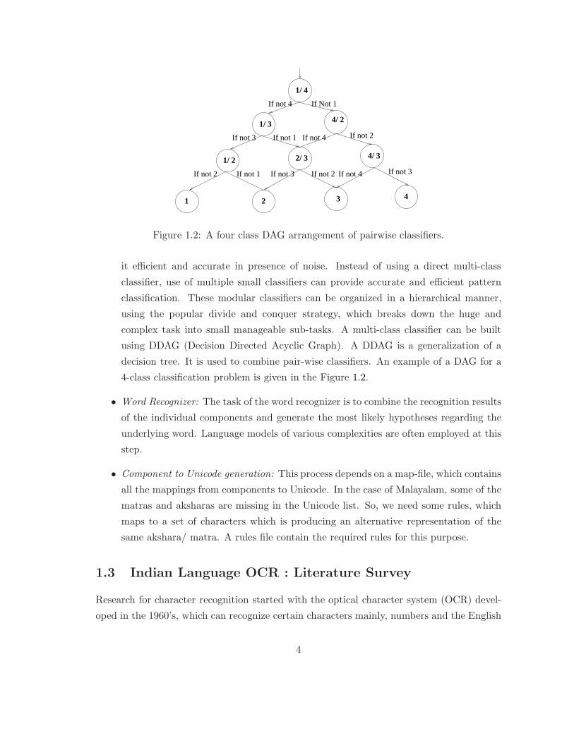
Figure 1.2: A four class DAG arrangement of pairwise classifiers.

it efficient and accurate in presence of noise. Instead of using a direct multi-class

classifier, use of multiple small classifiers can provide accurate and efficient pattern

classification. These modular classifiers can be organized in a hierarchical manner,

using the popular divide and conquer strategy, which breaks down the huge and

complex task into small manageable sub-tasks. A multi-class classifier can be built

using DDAG (Decision Directed Acyclic Graph). A DDAG is a generalization of a

decision tree. It is used to combine pair-wise classifiers. An example of a DAG for a

4-class classification problem is given in the Figure 1.2.

• Word Recognizer: The task of the word recognizer is to combine the recognition results

of the individual components and generate the most likely hypotheses regarding the

underlying word. Language models of various complexities are often employed at this

step.

• Component to Unicode generation: This process depends on a map-file, which contains

all the mappings from components to Unicode. In the case of Malayalam, some of the

matras and aksharas are missing in the Unicode list. So, we need some rules, which

maps to a set of characters which is producing an alternative representation of the

same akshara/ matra. A rules file contain the required rules for this purpose.

1.3 Indian Language OCR : Literature Survey

Research for character recognition started with the optical character system (OCR) devel-

oped in the 1960’s, which can recognize certain characters mainly, numbers and the English

4

alphabet. The use and applications of OCRs are well developed for most languages in the

world that use both Roman and non-Roman scripts [3, 4]. An overview on the last forty

years of technical advances in the field of character and document recognition is presented

by Fujisawa [5].

However, the optical character recognition for Indian languages is still an active research

area [6]. There are a large number of studies conducted on the recognition of Indian lan-

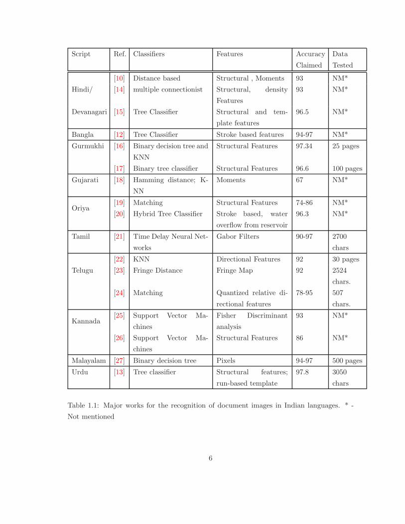
guages [7][8]. Summary of the works done are presented in Table 1.1. A comprehensive

review of Indian scripts recognition is reported by Pal and Chaudhuri [8]. A brief discus-

sion of some of the works on Indian scripts is reported in [9]. Structural and topological

features with tree-based and Neural Network classifiers are mainly used for the recognition

of Indian scripts.

Printed Devanagari character recognition has been attempted based on K-nearest neigh-

bor (KNN) and Neural Networks classifiers [10][11]. For classification purpose, the basic,

modified and compound characters are separated. Modified and basic characters are rec-

ognized by a structural features (such as concavities and intersections) based binary tree

classifier [10]. A hybrid of structural and run-based template features were used for the

recognition of compound characters. They reported an accuracy of 93%. Another study

with using Tree classifier and structural and template features reported an accuracy of

96.5% [11]. Both the cases did not mention the size of the test dataset.

These results were also extended to Bangla script [12][11]. A complete OCR system

for printed Bangla script is presented by Chaudhuri and Pal [12], where the compound

characters are recognized using a tree classifier followed by template-matching approach.

Stroke features are used to design the tree classifiers. The character unigram statistics

is used to make the the tree classifier efficient. Several heuristics are also used to speed

up the template matching approach. A dictionary-based error-correction scheme has been

integrated where separate dictionaries are compiled for root word and suffixes that contain

Morphy’s-syntactic information as well. The test dataset is not mentioned in this case.

A similar approach was tried for Urdu [13] in which a tree-classifier is employed for the

recognition of Urdu script after extracting a combination of topological, contour and water

reservoir features. It reports an accuracy of 97.8% on 3050 characters tested.

5

Script Ref. Classifiers Features Accuracy

Claimed

Data

Tested

Hindi/

[10] Distance based Structural , Moments 93 NM*

[14] multiple connectionist Structural, density

Features

93 NM*

Devanagari [15] Tree Classifier Structural and tem-

plate features

96.5 NM*

Bangla [12] Tree Classifier Stroke based features 94-97 NM*

Gurmukhi [16] Binary decision tree and

KNN

Structural Features 97.34 25 pages

[17] Binary tree classifier Structural Features 96.6 100 pages

Gujarati [18] Hamming distance; K-

NN

Moments 67 NM*

Oriya[19] Matching Structural Features 74-86 NM*

[20] Hybrid Tree Classifier Stroke based, water

overflow from reservoir

96.3 NM*

Tamil [21] Time Delay Neural Net-

works

Gabor Filters 90-97 2700

chars

Telugu

[22] KNN Directional Features 92 30 pages

[23] Fringe Distance Fringe Map 92 2524

chars.

[24] Matching Quantized relative di-

rectional features

78-95 507

chars.

Kannada[25] Support Vector Ma-

chines

Fisher Discriminant

analysis

93 NM*

[26] Support Vector Ma-

chines

Structural Features 86 NM*

Malayalam [27] Binary decision tree Pixels 94-97 500 pages

Urdu [13] Tree classifier Structural features;

run-based template

97.8 3050

chars

Table 1.1: Major works for the recognition of document images in Indian languages. * -

Not mentioned

6

Antanani and Agnihotri [18] reported character recognizer for Gujarathi script that uses

minimum Euclidean distance, hamming distance and KNN classifier with regular and Hu

invariant moments. The test dataset is not mentioned in this case.

Lehal and Singh reported a complete OCR system for Gurmukhi Script [16]. They use two

feature sets: primary features like number of junctions, number of loops, and their positions

and secondary features like number of endpoints and their locations, nature of profiles of

different directions. A multistage classifications scheme is used by combining binary tree

and nearest neighbor classifier. They supplement the recognizer with post-processor for

Gurmukhi Script where statistical information of Panjabi language syllable combinations,

corpora look-up and certain heuristics have been considered. They reports an accuracy of

96.6% on a test dataset of 100 pages.

An OCR system was also reported on the recognition of Tamil and Kannada script [28].

Recognition of Kannada script using Support Vector machine (SVM) has been proposed [29].

To capture the shapes of the Kannada characters, they extract structural features that

characterizes the distribution of foreground pixels in the radial and angular directions. The

size of test dataset is not mentioned in this case. A Tamil [21] OCR using Time Delay

neural Networks and Gabor Filters as feature, reports an accuracy of 90−97% on their test

dataset of 2700 characters in 2003.

For the recognition of Telugu script, Negi et al. [23] proposed a compositional approach

using connected components and fringe distance template matching. The system is tested

on 2524 characters and reported an accuracy of 92%. Another system is developed with

directional features and KNN as classifier reported an accuracy of 92%. Yet another Tel-

ugu OCR using quantized relative directional features and template matching reported an

accuracy of 78− 95% accuracy on 507 characters tested.

An OCR system for Oriya script was reported recently [19]. Structural features (such as

vertical line, number and position of holes, horizontal and vertical run code) are extracted for

modifiers (matra) and run length code, loop and position of hole for composite characters,

and a tree-based classification is developed for recognition. The system has been integrated

with spell checker with the help of dictionary and a huge corpus to post-process and improve

the accuracy of the OCR. Another OCR system for Oriya is reported with stroke based

features and template matching. Even though they report an accuracy of 96.3% and 74 −

86% respectively, these studies have not mentioned about the test dataset used.

An OCR system for Malayalam language is also available [27] in the year of 2003. A

two level segmentation scheme, feature extraction method and classification scheme, using

binary decision tree, is implemented. This system is tested on around 500 printed and

7

real pages, and report an accuracy of 94− 97%. Not enough technical details and analysis

available for this system.

Though there are various pieces of works reported by many research institutions, the

document analysis technology on Indian scripts is not so mature. This is attributed to the

existence of large number of characters in the scripts and their complexity in shape [7]. As

a result of which a bilingual recognition systems has been reported in recent past [11][30].

An OCR system that can read two Indian language scripts: Bangla and Devanagari (Hindi)

is proposed in [11]. In the proposed model, document digitization, skew detection, text line

segmentation and zone separation, word and character segmentation, character grouping

into basic, modifier and compound character category are done for both scripts by the same

set of algorithms. The feature sets and classification tree as well as the lexicon used for

error correction differ for Bangla and Devanagari. Jawahar et al. [30] presents character

recognition experiments on printed Hindi and Telugu text. The bilingual recognizer is

based on principal component analysis followed by support vector classification. Attempts

that focused on designing a hierarchical classifier with hybrid architecture [31], as well as a

hierarchical classifiers for large class problems [32] are also reported in the recent past.

1.4 Challenges

Compared to European languages, recognition of printed documents in Indian languages is a

more challenging task even at this stage. It becomes challenging because of the complexity

of the script, lack of resources, non-standard representations, and the magnitude of the

pattern recognition task. Sample paragraphs from various Indian languages are given in

the Figure 1.3. Some of the specific challenges are listed below.

• Large number of characters are present in Indian scripts compared to that of European

languages. This makes the recognition difficult for conventional pattern classifiers. In

addition, applications related to character recognition demand extremely high accu-

racy at symbol level. Something closer to perfect classification is often demanded.

• Complex character graphemes with curved shaped images and the added inflation

make the recognition difficult.

• Unicode/display/font related issues in building, testing and deploying working sys-

tems, slowed down the research in the development of character recognition system.

• Large number of similar/confusing characters: There are a set of characters which

8

Devanagiri

Telugu

Bangla

Kannada

Tamil

Oriya

Gujarati

Gurumukhi

Malayalam

Figure 1.3: Sample paragraphs from various Indian language books.

9

look similar to each other. The variation between these characters is extremely small.

Even humans find it difficult to recognize them in isolation. However, we usually read

them correctly from the context.

• Variation in glyph of a character with change in font/style: As the font or style changes

the glyph of a character also changes considerably, which makes the recognition diffi-

cult.

• Lack of standard databases, statistical information and benchmarks for testing, are

another set of challenges in developing robust OCRs.

• Lack of well developed language models, makes the conventional post-processor prac-

tically impossible.

• Quality of documents in terms of paper quality, print quality, age of document, the

resolution at which the paper is scanned etc. affects the pattern recognition con-

siderably. The document image may have undergone various kinds of degradations

like cuts, merges or distortion of the symbols, which reduces the performance of the

recognizers.

• Increased computational complexity and memory requirements due to large number

of classes, become a bottleneck in developing systems.

• Appearance of foreign or unknown symbols in the document makes the recognition

difficult, and sometimes unpredictable. Many of the Indian language documents have

foreign symbols present.

1.4.1 Challenges Specific to Malayalam Script

The recognition of printed or handwritten Malayalam has to deal with a large number of

complex glyphs, some of which are highly similar to each other. However, recent advances

in classifier design, combined with the increase in processing power of computers have all

but solved the primary recognition problem. The challenges in recognition comes from a

variety of associated sources:

• Non-Standard Font Design: The fonts used in Malayalam printing were mostly de-

veloped by artists in the individual publishing houses. The primary goal was to map

the ASCII codes to glyphs useful to typesetting the language and no standards were

adopted in both the character mapping as well as glyph sizes or aspect ratios. This

10

Cuts Merges

(a) Words with cuts and merges. (b) Merges in electronic typesetting.

Figure 1.4: Examples of cuts and merges in Malayalam printing.

introduced the problem of touching glyphs non-uniform gaps (see Figure 1.4) for many

character pairs in the electronic document itself, which gets transferred to the printed

versions. This makes the problem of word and character segmentation extremely dif-

ficult and error prone, and the errors are passed on to the recognition module. The

introduction of Unicode has standardized the font mappings for newly developed fonts.

However, the problem of standardizing glyph sizes still remains.

• Quality of Paper: To make the publications affordable to large portions of the society,

publications often use low quality paper in the printing process, even with offset

printing. The presence of fibrous substances in the paper used changes its ability

to absorb ink, resulting in large number of broken characters in print. The issues of

touching and broken characters are very difficult to handle for the recognition module.

• Script Variations: As mentioned in the previous section, the script in Malayalam

underwent a revision or simplification, which was partly reversed with the introduction

of electronic typesetting. This results in a set of documents that could contain either

the old lipi, the new lipi, or a mixture of the two. Any recognition system has to deal

with the resulting variety intelligently, to achieve good performance.

• Representation Issues: Another related problem is that of limitations in the initial

versions of Unicode, that prevented textual representations of certain glyphs. Unicode

did not have separate codes for chillus and they were created from non-vowel versions

of the consonants using ’ZWNJ’ ( Zero-Width Non-Joiner) symbols. This causes

substitution of one with the other in certain fonts, and can create significant differences

in meaning of certain words. However these issues have been resolved in Unicode 5.0

onwards.

11

• Compound Words and Dictionaries: A characteristic of the Malayalam language as

mentioned before is the common usage of compound words created from multiple root

words, using the sandhi rules. This creates a combinatorial explosion in the number

of distinct words in the language.

1.5 Overview of this work

The thesis mainly aims at addressing the problems character classification in Indian lan-

guages, giving a special emphasis to a south Indian language Malayalam. To ensure the

scalability and usability of the system, it is extremely important to test on a large dataset.

This work designs and implements methods for creating large dataset for testing and train-

ing of the recognition system. In the following sections we discuss the problem, contributions

of this work and organization of the thesis.

1.5.1 Contribution of the work

This thesis focuses on pattern classification issues associated with character recognition,

with special emphasis on Malayalam. We propose an architecture for the character classifi-

cation, and proves the utility of the the proposed method by validating on a large dataset.

The challenges in this work includes, (i) Classification in presence of large number of classes

(ii) Efficient implementation of effective large scale classification (iii) Performance analysis

and learning in large data sets (of Millions of examples).

The major contributions of this work are listed below.

1. A highly script independent dynamic programming (DP) based method to build large

dataset for testing and training character recognition systems.

2. Empirical studies on large dataset of various Indian languages to evaluate the perfor-

mance of state of the art classifiers and features on large datasets.

3. A hierarchical method to improve the computational complexity of SVM classifier for

large class problems.

4. An efficient design and implementation of SVM classifier to effectively handle large

class problems. The classifier module has employed for a OCR system for Malayalam.

5. The performance evaluations of the above mentioned methods on a large dataset.

We tested on a large dataset of twelve Malayalam books, which is more than 2000

document pages.

12

6. A novel system for adapting a classifier for recognizing symbols in a book.

1.5.2 Organization of the thesis

We start with building large datasets from real life documents for the efficient training and

testing of the system. In chapter 2, we propose script independent automatic methods for

creating such large datasets. The problem is to align a word image and its corresponding

text and label each components in the word image. We use a dynamic programing(DP)

based method to solve this problem.

Large number of pattern classifiers exist in the literature. It is important to study the

effectiveness of various state of the art classifiers on the character classification problem. We

empirically study the strengths of various classifier feature combinations on large datasets.

We present the results of our empirical study on character classification problem focusing

on Indian scripts, in Chapter 3. The dimensions of the study included performance of classi-

fiers using different features, scalability of classifiers, sensitivity of features on degradation,

generalization across fonts and applicability across five scripts etc.

Traditional pattern recognition literature aims at designing optimal classifiers for two

class classification problems. When the number of classes increases, problem becomes more

and more challenging, both conceptually as well as computationally. In Chapter 4, we

discuss the design and efficient implementation issues of the classifiers to handle large class

problems. We give focus on Support Vector Machines (SVM), which is proved to perform

the best in our empirical studies presented in chapter 3. In Chapter 5, we give various

performance achieved using the methods mentioned in the previous chapters.

In Chapter 6, we demonstrate a novel system for adapting a classifier for recognizing

symbols in a book. We employed a verification module as a post-processor for the classifier,

and make use of an automatic learning framework for the continuous improvement of clas-

sification accuracy. Finally, Chapter 7 presents the summary of contributions of this work,

possible directions of the work in future and the final conclusions.

13

14

Chapter 2

Building Datasets from Real Life

Documents

2.1 Introduction

The character recognition problem in Indian languages is still an active research area. One

of the major challenge in the development of such a system for Indian languages is the

lack of bench mark datasets for training and testing the classifier system. Because of

challenges involved in developing and handling a huge real life dataset, most of the research

are restricted with a small set of in-house dataset. Most of them employ synthetically

generated data for the experiments. But the experiments conducted on such a small or

syntactic data will not be statistically valid when the OCR is put upon a real testing

session with real life images. These OCRs fail drastically when they put for a practical

use. To trigger the research and development of highly accurate OCR, a large amount of

annotated data is necessary. The data with its corresponding labeling is called annotated

data. The annotated data is also called ground truth.

The ground truth can be generated in many ways providing annotation data with details

of different level granularity. During the annotation phase, different level of hierarchies

can be generated in the data set. That is, we can have corresponding text associated at

the page level, the paragraph level, the sentence level, the word level, and the character

or stroke level. Typically this annotation information is also very useful for segmentation

based routines that can also build up on their segmentation results so that they can further

improve. Refer [33] for further details on annotation which describes large scale annotation

of document images.

15

For the development of a classifier we need annotation at symbol level. Similar type

symbols will belong to a single class in the recognition. Availability of large collections of

labeled symbols plays a vital role in developing recognition techniques. In this chapter we

discuss a method to generate large dataset of labeled symbols, given a coarse (the word

level) annotated data. The problem is to align the word image and its corresponding text

and label each components in the word image. We use a dynamic programing(DP) based

method to solve this problem.

1 432 5 6 7 8 9 10 11 12

26 462 38, 110 55 28 57 53 37 146 55

Word image withactual symbolsmarked

(class−ids marked)symbol annotationWord image with

Word imagewith CCs marked

21 3 4 5 6 7 8 109 11 12

Merge Cut

(b)

(c)

(a)

Figure 2.1: (a) A word in Malayalam script, each symbol (connected component) is num-

bered. (b) The actual boundaries of the symbols. (c) The output of symbol annotation

algorithm based on DP method.

Figure 2.1 shows an example of symbol level annotation. In the Figure 2.1(a) we show

a word image with a cut and a merge. It has 12 connected components. Figure 2.1(b)

shows the actual symbol level annotation of the word, if the annotation is done manually.

It considers the two components of the cut character together and split the merged char-

acters at the appropriate position. Figure 2.1(c) shows the output of the DP based symbol

annotation algorithm. For the merge, since we do not know the exact position where the

merge has happened, we annotate the constituent symbols together and label the merged

symbols with the class-ids corresponding to the constituent symbols. On the other hand, a

cut symbol produces two or more connected components. These symbols together produce

the actual character. Therefore, we need to annotate these symbols or connected compo-

nents together and label them with a single class-id. In the next section we discuss the

challenges involved in solving the symbol annotation problem.

16

2.2 Challenges in Real-life Documents

A wide variety of degradations can exist in a real-life document image. Documents in digital

libraries are extremely poor in quality. The major challenges in alignment of word image

with its corresponding text in real-life document images can be broadly classified into three

levels, namely document level, content level and representational level.

2.2.1 Document level Issues

Document level challenges in generating such a huge dataset arise from the degradations

in the document image. An important aspect which directly affect the document quality is

the scanning resolution. Popular artifacts in printed document images include (a) Excessive

dusty noise, (b) Large ink- blobs joining disjoint characters or components, (c) Vertical

cuts due to folding of the paper, (d) Degradation of printed text due to the poor quality of

paper and ink or low scanning resolution, (f) Floating ink from facing pages, (e) back page

reflection etc [34]. Figure 2.2 shows examples of various degradations. Salt and pepper

noise is flipping the white pixels to black and the black pixels to white. The degradation

cut occurs when a group of black pixels from a component flipped to white pixel, so that

the component become two or more pieces. Similarly merge is a degradation that a group

of white pixels at a region flipped to black, so that two or more components get connected.

back page reflection

ink blob

distortion

cut

merges

Figure 2.2: Example word images of various degradations from the book “Marthandavarma”

(Malayalam script).

Some of the degradations can occur during preprocessing. During thresholding the image,

if the threshold is low, it might increase the number of cuts and if the threshold is high, the

number of merges in the components might increase. The thickness of the character image

might be different in different portions of the image. This can happen either during scanning

17

or some portions of the pages might be dull even in the original document itself. Using a

global threshold might increase the degradation of such pages. Some of the punctuations,

if it is very small in size, might be taken away from the image during noise cleaning.

The density of the page is another aspect which decides the document quality. If the

character spacing in the words is too low the chances of merges in the components are high.

In the new digitalized type settings the character spacing of the documents can be varied

from font to font and word-processor to word-processor.

2.2.2 Content level Issues

There are various content level issues comes into picture when we deal with real life docu-

ments.

• Presence of foreign language content: It is very common to see English words in

between an Indian language script content. It is common to see the English word

written in the Indian script also. The mathematical symbols or rare punctuations are

also considered as foreign symbols.

• Violation of language rules: We could find the examples of character combinations,

which is not possible by the language rules in the text. These types of combinations

occur when the content is specific to any regional slang of the language or when some

vocal expressions has to be expressed (e.g. exclamation sounds) in a different way.

This can be considered as a language and author or book type specific problem.

• Invalid typesetting: The problem with invalid typesetting occurs when the word pro-

cessor uses some ASCII font for the typesetting. These may cut a word where by

language rules the word should not be cut. An example is, consider the situation of

a character where the modifier attached to that character appears in the left most

portion of a line. The modifier does not have an independent existence by language

rules. But, using invalid typesetting it is possible to put a newline in between the

modifier and the character to which the modifier attached to.

2.2.3 Representational level Issues

Images of the same words that occur at different places of the same book or a different book

differ in a number of ways due to pixel variations, noise, changes in font face, font type and

font size etc. Even in the same page the same characters might be written differently.

Most popular example is the presence of a header in a different font, style or/and size, or

18

a presence of a drop cap which is much bigger in size etc. A description or representation

is required for the words of the documents which will allow matching in spite of these

differences.

Building an appropriate description is critical to the robustness of the system against

signal noise. In general, color, shape or/and texture features are used for characterizing the

content. More specific features are required for word representation in document images.

These features can be more specific to the domain as they contain an image-description

of the textual content in it. It is observed that many of the popular structural features

work well for good quality documents. Word images, particularly from newspapers and old

books, are of extremely poor quality. Common problems in such document databases will

have to be analyzed before identifying the relevant features. We use structural, profile and

scalar features for effectively representing and matching the word images. More explanation

on these features are given in the Subsection 2.7.1.

In the following Section 2.3 we give a brief explanation about standard dynamic pro-

gramming(DP) algorithm. This is followed by the explanation (in Sections 2.4, 2.5 and 2.6

) of how a modified version of DP based algorithm is used for the alignment of word with

its corresponding text.

2.3 Background on Dynamic Programming

Dynamic programming is a method of solving problems that exhibit the properties of over-

lapping sub problems and optimal substructure. A problem is said to have overlapping sub

problems if it can be broken down into sub problems which are reused multiple times. For

example, the problem of calculating the nth Fibonacci number does, however, exhibit over-

lapping sub problems. The problem of calculating fib(n) thus depends on both fib(n− 1)

and fib(n− 2), where fib(x) is the function to calculate xth Fibonacci number.

A problem is said to have optimal substructure if the globally optimal solution can be

constructed from locally optimal solutions to sub-problems. The general form of problems

in which optimal substructure plays a roll goes something like this. Let’s say we have a

collection of objects called A. For each object O in A we have a “cost” C(O). Now find the

subset of A with the maximum (or minimum) cost, perhaps subject to certain constraints.

The brute-force method would be to generate every subset of A, calculate the cost, and

then find the maximum (or minimum) among those values. But if A has n elements in it

we are looking at a search space of size 2n if there are no constraints on A. Often n is huge

making a brute-force method computationally infeasible.

19

There are several algorithms which use dynamic programming. String matching, Viterbi

Algorithm used for hidden Markov models, Floyd’s All-Pairs shortest path algorithm, Travel

ling salesman problem are a few examples. Lets look at a worked out example to get a feel

of Dynamic Programming.

2.3.1 A worked out Example - String Matching

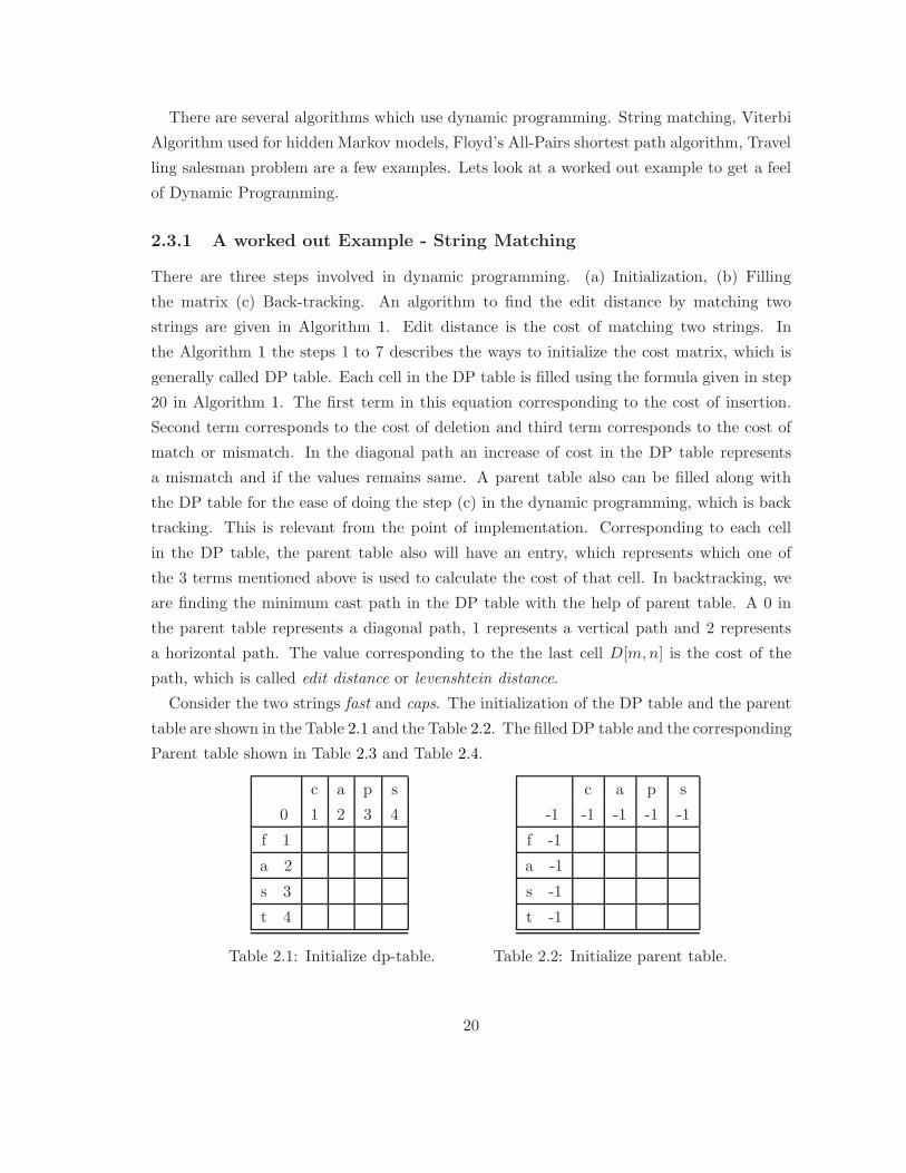
There are three steps involved in dynamic programming. (a) Initialization, (b) Filling

the matrix (c) Back-tracking. An algorithm to find the edit distance by matching two

strings are given in Algorithm 1. Edit distance is the cost of matching two strings. In

the Algorithm 1 the steps 1 to 7 describes the ways to initialize the cost matrix, which is

generally called DP table. Each cell in the DP table is filled using the formula given in step

20 in Algorithm 1. The first term in this equation corresponding to the cost of insertion.

Second term corresponds to the cost of deletion and third term corresponds to the cost of

match or mismatch. In the diagonal path an increase of cost in the DP table represents

a mismatch and if the values remains same. A parent table also can be filled along with

the DP table for the ease of doing the step (c) in the dynamic programming, which is back

tracking. This is relevant from the point of implementation. Corresponding to each cell

in the DP table, the parent table also will have an entry, which represents which one of

the 3 terms mentioned above is used to calculate the cost of that cell. In backtracking, we

are finding the minimum cast path in the DP table with the help of parent table. A 0 in

the parent table represents a diagonal path, 1 represents a vertical path and 2 represents

a horizontal path. The value corresponding to the the last cell D[m,n] is the cost of the

path, which is called edit distance or levenshtein distance.

Consider the two strings fast and caps. The initialization of the DP table and the parent

table are shown in the Table 2.1 and the Table 2.2. The filled DP table and the corresponding

Parent table shown in Table 2.3 and Table 2.4.

c a p s

0 1 2 3 4

f 1

a 2

s 3

t 4

Table 2.1: Initialize dp-table.

c a p s

-1 -1 -1 -1 -1

f -1

a -1

s -1

t -1

Table 2.2: Initialize parent table.

20

Algorithm 1 int EditDistance(char (s[1..m], char t[1..n])

1: #define MATCH 0

2: #define INSERT 0

3: #define DELETE 0

4: declare struct D[0..m, 0..n]

5: for i = 1 to m do

6: D[i, 0].cost := i

7: D[i, 0].parent := −1

8: end for

9: for j = 1 to n do

10: D[j, 0].cost := j

11: D[i, 0].parent := −1

12: end for

13: for i = 1 to m do

14: for j = 1 to n do

15: if s[i] = t[j] then

16: cost = 0

17: else

18: cost = 1

19: end if

20: D[i, j].cost = min{

D[i− 1, j] + 1, //insertion

D[i, j − 1] + 1, //deletion

D[i− 1, j − 1] + cost//substitution

21: D[i, j].parent = argmin{

D[i− 1, j] + 1(INSERT ), //insertion

D[i, j − 1] + 1(DELETE), //deletion

D[i− 1, j − 1] + cost(MATCH)//substitution

.

22: end for

23: end for

24: return D[m,n]

21

c a p s

0 1 2 3 4

f 1 1 2 3 4

a 2 2 1 2 3

s 3 3 2 2 2

t 4 4 3 2 3

Table 2.3: Fill dp-table.

c a p s

0 -1 -1 -1 -1

f -1 0 1 1 1

a -1 2 0 1 1

s -1 2 2 0 0

t -1 2 2 0 1

Table 2.4: Fill parent table.

The value 0 in the parent table indicates that the parent of that cell is diagonally con-

nected to the particular cell. This corresponds to a match or a mismatch. The value 1 in the

parent table indicate that the parent is vertically connected to the cell, which means that

an insert has occurred. Similarly, the value 2 in the parent cell indicates the a horizontal

connection and represents a delete. The lowest cost path is shown in color in the Table 2.5

and the Table 2.6.

c a p s

0 -1 -1 -1 -1

f -1 0 1 1 1

a -1 2 0 1 1

s -1 2 2 0 0

t -1 2 2 0 1

Table 2.5: Backtracking using parent

table.

c a p s

0 1 2 3 4

f 1 1 2 3 4

a 2 2 1 2 3

s 3 3 2 2 2

t 4 4 3 2 3

Table 2.6: Alignment path in the DP-

table.

The match string and the alignment of the two words are shown in the Figure 2.3.

S − MismatchM − Match

I − InsertD − Delete

Matching String : SMDMIf a s t

c a p s

Figure 2.3: Example-1 of string alignment.

22

2.4 A Naive Algorithm to Align Text and Image for English

The word(text) and word image alignment attempts to search the best match between each

character in the text with the corresponding component in the image. We use dynamic pro-

gramming based approach to solve this problem. The problem is to find a global alignment

between the text and word image, and label each component in the word image with the

corresponding text. The problem is tough in the presence of noise, degradations, cuts and

merges in the components etc.

We solve the problem in the image domain. For this the text has to be rendered (using a

rendering engine) to get the corresponding image. This image is called rendered word image,

say R. We have to label each component in R with the corresponding text. This can be done

easily for English by finding the connected components in the word image. The connected

components has to be sorted with respect to its left coordinate to get the components in

order. Once this is done, the labeling will be sequential, since most of the characters in

English are composed of only one component. We need to take care of characters like i and

j and punctuations like colon(:), semicolon (;), question mark (?), exclamation mark(!),

double quote(”), percentile symbol (%), and equal to (=). Now we have two word images, R

and the original word image, say W . Our problem is now to align R and W and propagate

the labeling of components in R to the corresponding components in W .

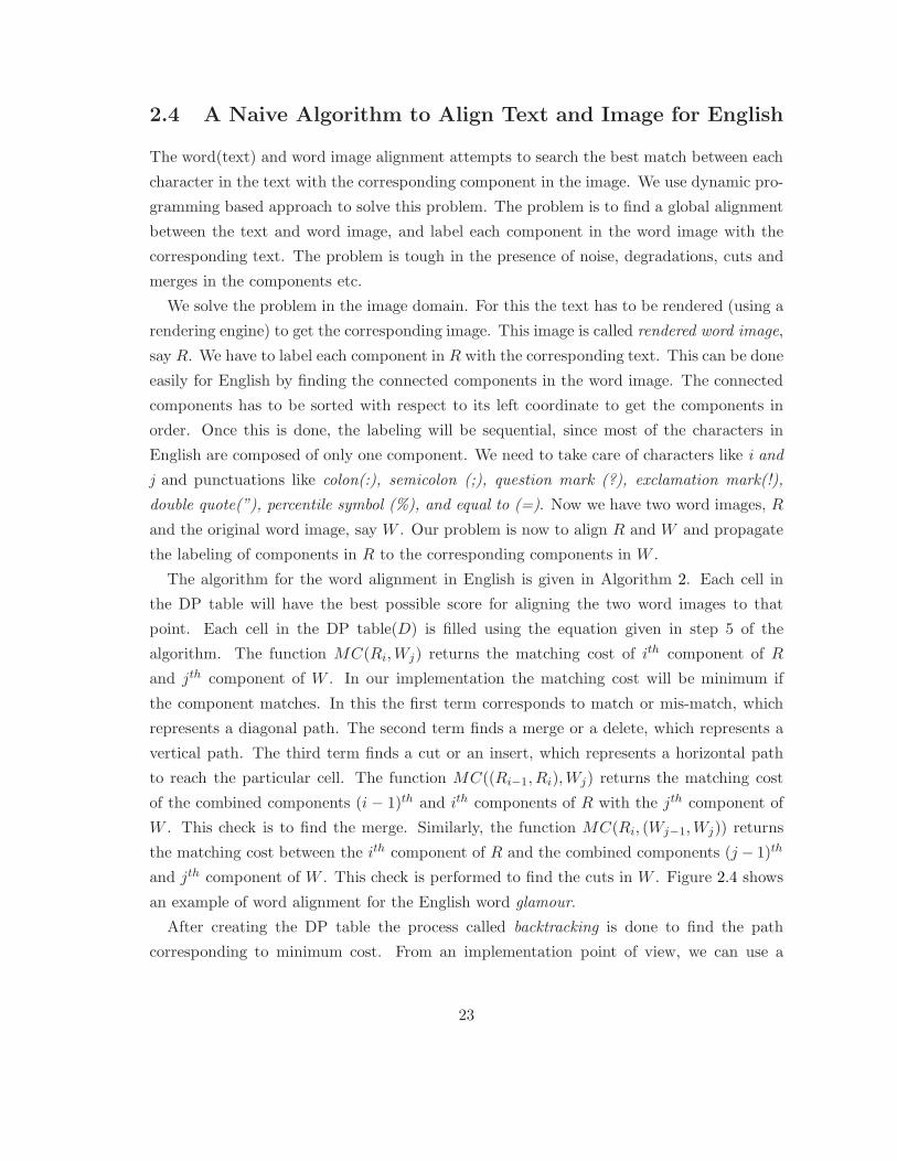
The algorithm for the word alignment in English is given in Algorithm 2. Each cell in

the DP table will have the best possible score for aligning the two word images to that

point. Each cell in the DP table(D) is filled using the equation given in step 5 of the

algorithm. The function MC(Ri,Wj) returns the matching cost of ith component of R

and jth component of W . In our implementation the matching cost will be minimum if

the component matches. In this the first term corresponds to match or mis-match, which

represents a diagonal path. The second term finds a merge or a delete, which represents a

vertical path. The third term finds a cut or an insert, which represents a horizontal path

to reach the particular cell. The function MC((Ri−1, Ri),Wj) returns the matching cost

of the combined components (i − 1)th and ith components of R with the jth component of

W . This check is to find the merge. Similarly, the function MC(Ri, (Wj−1,Wj)) returns

the matching cost between the ith component of R and the combined components (j − 1)th

and jth component of W . This check is performed to find the cuts in W . Figure 2.4 shows

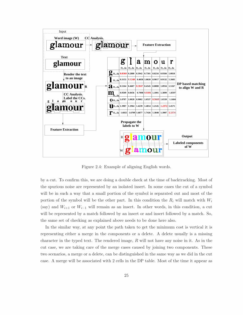
an example of word alignment for the English word glamour.

After creating the DP table the process called backtracking is done to find the path

corresponding to minimum cost. From an implementation point of view, we can use a

23

Algorithm 2 DP based algorithm to align text and image for English

1: Input: Word image W and the corresponding text from annotation.

2: Render the text to get a word image R, and label each component, with the

corresponding character in the text.

3: Find the connected components in the original word image.

4: Initialize the dynamic programming table D of size m× n, where (m− 1) and (n − 1)

are the no. of connected components in R and W respectively.

5: Fill each cell, D(i, j) in the table using the following equation.

D(i, j) = min

D(i− 1, j − 1) + MC(Ri,Wj)

D(i− 1, j) + MC((Ri−1, Ri),Wj)

D(i, j − 1) + MC(Ri, (Wj−1,Wj))

where, MC(Ri,Wj) is the matching Cost of symbol Ri in the text(rendered as image)

with symbol Wj in the original image.

6: Get the matching String by reconstructing the path, by following the minimum cost

path.

7: Propagate the labels of symbols in R to W .

Parent table to make this process faster. The purpose of the parent table is described in

the previous section. At each point, we need to identify possibilities for match, mis-match,

insert, delete, cut and merge. In the matching string, if at a point the path taken to get the

minimum cost is diagonal, there are two interpretations for it. Either it will be a match or a

mis-match. We use a threshold to distinguish between match and mis-match. A mis-match

can be either a typing mistake in the annotated text or the appearance of a character which

is having high featural match with the character in the word image. We selected 0.4 as

the threshold, if the matching cost is less than the threshold we consider it as a match,

otherwise a mismatch. The threshold is chosen by statistical analysis of the data.

At any point, if the path taken to get the minimum cost is horizontal it represents either

a cut in the components or an insert. The presence of spurious noise is considered as a

noise the word image. Another chance of insert is an additional character in the typed

text. At this stage we are taking care of only the cases of a single cut, which makes the

component into two pieces. These two scenarios, a cut or an insert, can be distinguished

by the following way. The cut will be associated with two cells in the DP table, which will

contribute two entries to the matching string. Most of the time, a sequence like, a mis-

match followed by an insert or an insert followed by a mismatch would have been resulted

24

Render the textto an image

romalg u

glamourText

Word image (W)

Feature Extraction

Feature Extraction

0.4050 1.0020

0.8000 1.0934

0.9509 0.8456 0.70980.9391 1.1001

1.0787 1.0028 1.1684

1.4575

1.6025 1.6709 1.3848 1.39071.74261.6877

1.3987 1.1964 1.4239 1.4014

1.03390.9669

1.2145

1.05370.9002

1.3899 1.8597

1.51670.45450.5164

0.3153

0.4607

0.9017 0.9132 1.2603

1.08180.95840.82160.75010.39420.2880

1.5374

1.2372

0.0360

0.1240

0.3047

R

W

Propagate the labels to W

Labeled components of W

Output

DP based matchingto align W and RR

Input

f1,..fn

f1,..fn

f1,..fn

f1,..fn

f1,..fn

f1,..fn

f1,..fn

f1,..fn f1,..fn f1,..fn f1,..fn f1,..fn f1,..fn f1,..fn

CC Analysis.Label the CCs.

CC Analysis.

Figure 2.4: Example of aligning English words.

by a cut. To confirm this, we are doing a double check at the time of backtracking. Most of

the spurious noise are represented by an isolated insert. In some cases the cut of a symbol

will be in such a way that a small portion of the symbol is separated out and most of the

portion of the symbol will be the other part. In this condition the Ri will match with Wi

(say) and Wi+1 or Wi−1 will remain as an insert. In other words, in this condition, a cut

will be represented by a match followed by an insert or and insert followed by a match. So,

the same set of checking as explained above needs to be done here also.

In the similar way, at any point the path taken to get the minimum cost is vertical it is

representing either a merge in the components or a delete. A delete usually is a missing

character in the typed text. The rendered image, R will not have any noise in it. As in the

cut case, we are taking care of the merge cases caused by joining two components. These

two scenarios, a merge or a delete, can be distinguished in the same way as we did in the cut

case. A merge will be associated with 2 cells in the DP table. Most of the time it appear as

25

a mismatch followed by a delete or a delete followed by a mismatch. We are double checking

to verify whether it is a merge during backtracking. If it is, the components will be marked

as merged components other wise it will be considered as a delete. Also an isolated delete

will be considered as a delete. As explained in the case of cuts, sometimes a match followed

by delete or a delete followed by a match can also be a merge. This also needs to be taken

care while backtracking.

2.5 Algorithm to Align Text and Image for Indian Scripts

In this section we discuss about how the Algorithm 2 can be extended to fit Indian language

scripts. Aligning Indian language scripts is a much more difficult problem compared to

English. One reason is the size of the problem. The total number of characters present in

English are around 70. In the case of any Indian languages it comes out to be in the order

of hundreds. There are also many similar characters present in this set. We need to use

more features to get proper match between the components.

Languages like English have characters as their building blocks. The smallest entity that

can be easily extracted from a document in such language is the character. Indian scripts

have oriented from the ancient Brahmi script which is phonetic in nature. Thus in Indian

languages, syllables form the basic building blocks. If all the syllables are considered as

independent classes and recognized, a very large amount of information has to be stored.

This creates the need for splitting syllables into their constituent components, which is not

a trivial task.

In other words, the challenge comes from the definition of text(Unicode) used to annotate

the word image. Before going to the details we will define the basic terminologies that is

used to describe the problems.

• Character: is an entity used in a data exchange.

• Glyph: is a particular shape of a character and part of a character. Glyphs can have

variations with font to font.

• Unicode: provides a unique number for every character, no matter what the platform,

no matter what the program, no matter what the language.

• Component/Symbol: connected component(CC) present in the glyph of a character.

These terminologies have a broader meaning in the context of Indian languages compared

to English language. In English a character represents a single alphabet. A character,

26

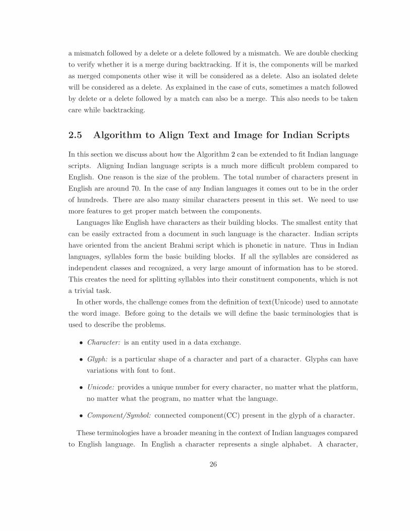
Algorithm 3 DP based algorithm to align text and image for Indian Languages

1: Input: Word image W and the corresponding Unicode/text from annotation.2: convert the Unicode to the class labels using a map file MAP .3: Reorder the symbols, using the language rules in the RULES file.4: Render the symbols to get a word R, and label each symbol with the corresponding class label.5: Find the connected components in the original word image.6: Initialize the dynamic programming table D of size m × n, where (m − 1) and (n − 1) are the

no. of connected components in R and W respectively.7: Fill each cell, D(i, j) in the table using the following equation.

D(i, j) = min

D(i− 1, j − 1) + MC(Ri, Wj)D(i− 1, j) + MC((Ri−1, Ri), Wj)D(i, j − 1) + MC(Ri, (Wj−1, Wj))

where, MC(Ri, Wj) is the matching Cost of symbol Ri in the text(rendered as image) withsymbol Wj in the original image.

8: Get the matching String by reconstructing the path, by following the minimum cost path.9: Propagate the labels of symbols in R to W .

Unicode, glyph or a component/symbol is representing a single entity in English. Each

character in English has its corresponding Unicode. Most of the characters in English can

be represented using a single glyph. Most of the glyphs in English are single component.

However, there are a few exceptions like the character ‘i’ and ‘j’, which composed of 2

components. There are one to one mappings between Unicode, characters, glyphs and

components.

But in the case of Indian languages, all these four terminologies mentioned above has

different meaning. A character is called akshara in Indian context. It can be any combina-

tion of cv, ccv or cccv sequences where c stands for consonant and v stands for vowel. An

akshara can be represented using a single or multiple Unicode. Similarly to represent an

akshara we might use single glyph or multiple glyphs. An akshara might consists of single

or multiple components. Also, a single component can represent multiple Unicode and a

single Unicode can represent multiple components.

Considering all these facts, given a word image and its corresponding text in Unicode,

the labeling of the connected components with the text is not trivial as we did in English.

We are tackling this problem by converting the Unicode text to symbol level, which is a

proprietary numbering which has a unique representation for all the existing symbols in that

particular language. Each symbol will be composed of either a single Unicode or multiple

Unicode. The conversion from symbol to Unicode is trivial when it comes in a single unit.

So, if we get a labeling at symbol level, that is good enough.

The conversion from Unicode to symbols uses a MAP FILE, which maps each Unicode to

27

its corresponding symbol representations, which is called class labels. We need to represent

the symbols in the order in which it appears in the word image. A trivial mapping of a

Unicode word will not give us this order. This is again because of the specialties in which

Indian scripts are represented using Unicode. Suppose we have a modifier, (called Matra

in Indian context ) symbol. The modifier can appear on the right, left, top or bottom of

a character. Sometimes it come as a modification to the base character. Which ever way

it actually appears in the script, the Unicode follows a common rule to represent a matra,

that is, the Unicode that represents a Matra appears after the Unicode of the character to

which the Matra is associated. It is the responsibility of the font to put the symbols in the

right place it should appear. Unfortunately most of the popular Unicode fonts are not doing

this job correctly at present. There are errors in the order in which these fonts displays

the characters. As a result most of the rendering engines (QT or ImageMagick) are not

able to render the words correctly. We use language rules for the reordering of the symbols

to get it in the correct order as it appears in the image, with the help of a RULES FILE.

Also, Unicode represents the conjunct symbols using more than one Unicode. A group of

Unicode (usually a group of 3), might be representing another symbol representation in the

language. For the conversion of this case also the RULES FILE is used.

We use our own implementation for rendering the Unicode to get the corresponding

rendered word image. The labeling of each component is done in the class label level.

Once we get the the labeled rendered word image(R), the rest of the algorithm proceeds as

discussed in the previous section. Algorithm 3 explains the modified dynamic programming

based algorithm to align word and Unicode in Indian scripts.

The method that we employ is a generic one that can be used for any Indian language.

The language specific files, MAP FILE and RULES FILE have to be changed when we

change the language. Also, since the rendering is proprietary, the rules, which specifies the

positioning of the matras, used for rendering also need to changed from script to script. We

use language independent structural features for matching the components. So, the same

set of features will be sufficient for any Indian language. The method is generic in such

a way that, we can add another feature to improve the performance of matching module.

Figure 2.5 shows an example of word alignment in the Malayalam script.

2.6 Challenges for Degraded Documents

In this section we will discuss how the degradation in the document images are handled in

the Algorithm 3. The major degradations include cuts in the components, merges in the

28

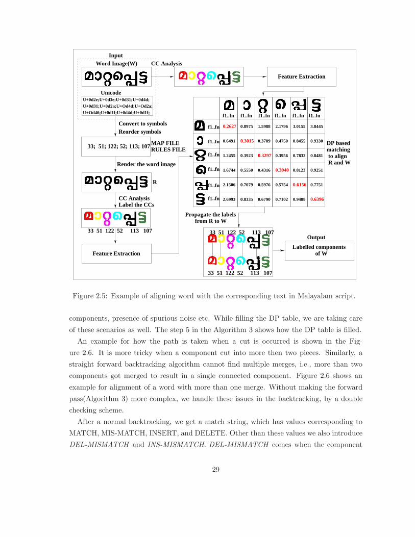
Feature Extraction

Feature Extraction

f1..fn f1..fn f1..fn f1..fn f1..fn f1..fn

1.5988

0.9330

0.7751

0.6491

1.2455

1.6744

2.1506

2.6993

0.8975

0.3923

0.5550

0.7079

0.3789

0.4316

0.5976

0.67900.8335

2.1796

0.4750

0.3956

0.5754

0.7102

3.0155

0.8455

0.7832

0.8123

0.6156

0.9488

3.8445

0.8481

0.9251

0.6396

0.3940

0.3297

0.3015

0.2627f1..fn

f1..fn

f1..fn

f1..fn

f1..fn

f1..fn

33 51 122 52 113 107

33 51 122 52 113 107

Propagate the labelsfrom R to W

Labelled componentsof W

DP basedmatchingto alignR and W

Word Image(W)Input

Convert to symbolsReorder symbols

33; 51; 122; 52; 113; 107

R

Render the word image

Label the CCsCC Analysis

33 51 122 52 113 107

CC Analysis

Output

U+0d2e;U+0d3e;U+0d31;U+0d4d;U+0d31;U+0d2a;U+Od4d;U+Od2a;U+Od46;U+0d1f;U+0d4d;U+0d1f;

Unicode

RULES FILEMAP FILE

Figure 2.5: Example of aligning word with the corresponding text in Malayalam script.

components, presence of spurious noise etc. While filling the DP table, we are taking care

of these scenarios as well. The step 5 in the Algorithm 3 shows how the DP table is filled.

An example for how the path is taken when a cut is occurred is shown in the Fig-

ure 2.6. It is more tricky when a component cut into more then two pieces. Similarly, a

straight forward backtracking algorithm cannot find multiple merges, i.e., more than two

components got merged to result in a single connected component. Figure 2.6 shows an

example for alignment of a word with more than one merge. Without making the forward

pass(Algorithm 3) more complex, we handle these issues in the backtracking, by a double

checking scheme.

After a normal backtracking, we get a match string, which has values corresponding to

MATCH, MIS-MATCH, INSERT, and DELETE. Other than these values we also introduce

DEL-MISMATCH and INS-MISMATCH. DEL-MISMATCH comes when the component

29

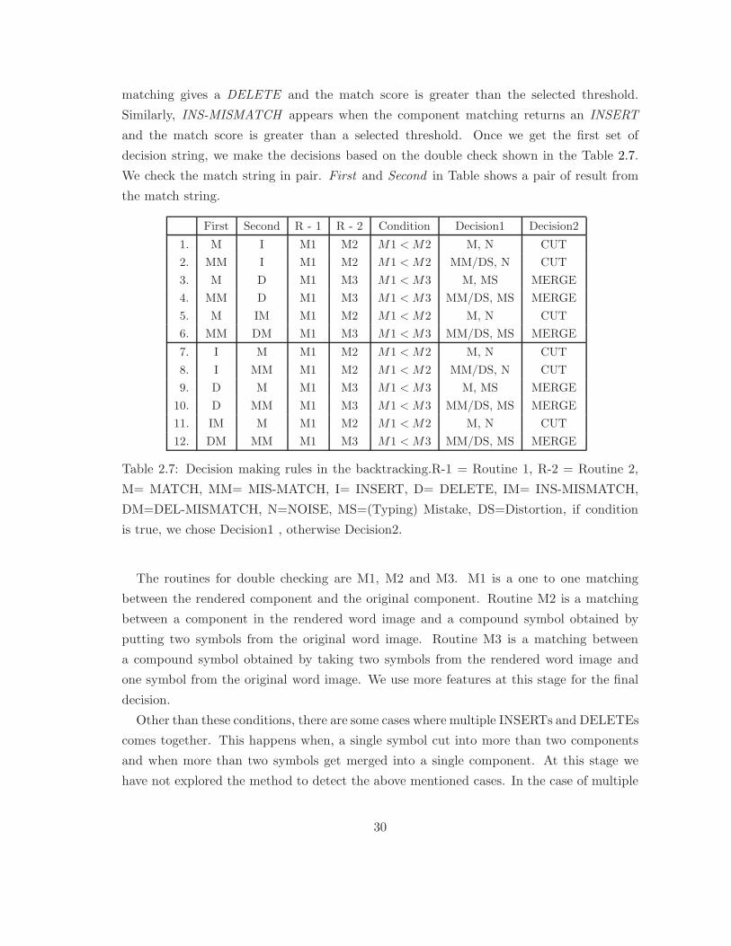
matching gives a DELETE and the match score is greater than the selected threshold.

Similarly, INS-MISMATCH appears when the component matching returns an INSERT

and the match score is greater than a selected threshold. Once we get the first set of

decision string, we make the decisions based on the double check shown in the Table 2.7.

We check the match string in pair. First and Second in Table shows a pair of result from

the match string.

First Second R - 1 R - 2 Condition Decision1 Decision2

1. M I M1 M2 M1 < M2 M, N CUT

2. MM I M1 M2 M1 < M2 MM/DS, N CUT

3. M D M1 M3 M1 < M3 M, MS MERGE

4. MM D M1 M3 M1 < M3 MM/DS, MS MERGE

5. M IM M1 M2 M1 < M2 M, N CUT

6. MM DM M1 M3 M1 < M3 MM/DS, MS MERGE

7. I M M1 M2 M1 < M2 M, N CUT

8. I MM M1 M2 M1 < M2 MM/DS, N CUT

9. D M M1 M3 M1 < M3 M, MS MERGE

10. D MM M1 M3 M1 < M3 MM/DS, MS MERGE

11. IM M M1 M2 M1 < M2 M, N CUT

12. DM MM M1 M3 M1 < M3 MM/DS, MS MERGE

Table 2.7: Decision making rules in the backtracking.R-1 = Routine 1, R-2 = Routine 2,

M= MATCH, MM= MIS-MATCH, I= INSERT, D= DELETE, IM= INS-MISMATCH,

DM=DEL-MISMATCH, N=NOISE, MS=(Typing) Mistake, DS=Distortion, if condition

is true, we chose Decision1 , otherwise Decision2.

The routines for double checking are M1, M2 and M3. M1 is a one to one matching

between the rendered component and the original component. Routine M2 is a matching

between a component in the rendered word image and a compound symbol obtained by

putting two symbols from the original word image. Routine M3 is a matching between

a compound symbol obtained by taking two symbols from the rendered word image and

one symbol from the original word image. We use more features at this stage for the final

decision.

Other than these conditions, there are some cases where multiple INSERTs and DELETEs

comes together. This happens when, a single symbol cut into more than two components

and when more than two symbols get merged into a single component. At this stage we

have not explored the method to detect the above mentioned cases. In the case of multiple

30

cut of a component, now we find only two pieces as a part of that component and the rest

of the pieces are considered as spurious noise. And similarly, we consider only two merge

at a place, and the rest of the components will be counted to deletes. Still we can extend

the backtracking method to find multiple cuts and merges on a component.

Another important challenge in the alignment of word image with the rendered word is

the change in the font used to render the word. If the font in the original word image is

very different from the font used to render the word, especially in the case of fancy fonts

(headers of the book), the matching may go wrong. To solve these problem we may need

to work at the feature level.

2.7 Implementation and Discussions

2.7.1 Features for matching

Effective features for word matching should take care the popular artifacts discussed in

the Subsection 2.2.1 that can occur in the word images. We found that three categories

of features are effective for addressing these artifacts. The features could be a sequential

representation of the word shape, content or a structural representation of the word image.

We employ a combination of scalar, profile, structural features used in [35, 36, 37]. The

images we operate on are all binary with two intensity levels [0, 255]. We refer to an image

of height h as I(r, c), where r and c indicate the row and column, respectively, index of the

pixel.

Scalar Features:

Scalar features include an estimate of the number of ascenders and descenders in the image,

the aspect ratio of the image, and number of loops in the image.

Profile Features:

The profile features include projection profiles, background to ink transitions, upper and

lower word profiles.

Projection profile: It is a measure of ink distribution of the word image. Each value

in the profile is calculated by summing over the pixel values in the corresponding image

column is given by

pp(I, c) =h

∑

k=1

(255 − I(r, c)) (2.1)

31

0.9532 1.14650.6465 0.7790 1.3600 1.6078 1.8165

0.5250

0.7059

1.2614 0.6191

0.8134 0.3014 0.4798 0.6907 0.7724 0.9679 1.1357 1.2410

0.9265 0.7996 0.64430.3887 0.6823 1.0358 1.2097 1.4698 1.9168

1.0939 1.1740 0.7266 0.4977 0.5651 0.9907

1.4926 0.8301 1.1196 0.58640.6667 0.8347 0.9833

1.4507 1.8092 1.0517 0.7129 0.7193 0.85730.8145 0.8737

0.7691 0.7338 1.0274 1.2984 1.5839 1.9494 2.3965

0.4236

1.13310.8166

0.9039

0.8311

0.1366

0.2304

0.4977 + MC( R( ), W( ) ) = 0.5651

0.6823 + MC( R( ) , W ( ) ) = 1.4652{{{ {

{{

= 0.5651

1.0358 + MC( R( ), W( ) ) = 2.3459

=Minimum

Feature Extraction

Propagate the labels from R to W

Rendered Word Image (R) Word Image (W)

CC Analysis16 55 35 55 101 57 9Label

14 55 35 55 101 57 9

DP basedAlignment

f1 .. fn f1 .. fn f1 .. fn f1 .. fn f1 .. fn f1 .. fn f1 .. fn f1 .. fn f1 .. fn

f1 .. fn

f1 .. fn

f1 .. fn

f1 .. fn

f1 .. fn

f1 .. fn

f1 .. fn

14 55 35 55 101 101 57 9 9

Figure 2.6: Example of aligning word with two cuts.

Figure 2.8 shows the plot of a typical projection profile. We invert the image before

the calculation, causing concentrations of ink to create peaks, because we would like to

measure the ink contained in each column. The descriptive power of the modied profile

32

Feature Extraction

Propagate the labels from R to W

CC Analysis

Rendered Word Image (R) Word Image (W)

AlignmentDP based

0.8032 1.1895 1.5318 1.8417 2.1886 2.4068

1.1354 1.3356 1.4622 2.0569 2.6310 2.7503

0.8579 0.7810 0.9603 1.2099 1.3747 1.8787

2.3007 2.2585 2.0051 2.0249 1.8020 1.8824

1.0520

1.1666

1.4322

1.7886

2.0392 1.7265

1.5261

1.3780

0.9901

0.7853

1.7031

1.5014

1.4077

0.9398

1.4904 1.9453 2.0514

1.2363 1.5833 1.6614

1.0164 1.1432 1.3219 1.7282

2.0524 1.3401 1.7355

1.5310 1.2390 2.0424

f1 .. fn f1 .. fn f1 .. fn f1 .. fn f1 .. fn f1 .. fn f1 .. fn

f1 .. fn

f1 .. fn

f1 .. fn

f1 .. fn

f1 .. fn

f1 .. fn

f1 .. fn

f1 .. fn

f1 .. fn 1.4421

1.3361

1.1236

1.0631

0.9264

0.7499

0.6789

0.6557

0.3660

{

{{= Minimum 1.4077 + MC ( R( ) + W ( ) ) = 2.4357

0.9398 + MC( R( ) + W ( ) ) = 1.7562

{{{

0.9264 + MC( R( ) + W ( ) ) = 1.1061

= 1.1061

37 55 107 57 37 58 43 63 14

37 55 107 57 37 58 43 63 14

Label 37 55 107 57 37 58 43 63 14

Figure 2.7: Example of aligning word with two merges.

33

remains unchanged.

(b) Projection from upper boundary of each CC in the word

(c) Projection from lower boundary of each CC in the word

(a) A malayalam word image

(e) Lower word profile (d) Upper word profile

Figure 2.8: Projection Profiles.

Ink transition: Ink transition represent the internal shape of the image, computed by

counting the number of transitions from background (paper) to ink for every column of the

image (see Figure 2.8).

Structural Features:

The structure of the word image is described by statistical moments and region-based mo-

ments. Each moment order carries different structural information about the same image.

Many of the pattern recognition problems are addressed used different moment orders. Nor-

malized moments, such as first-order moments (M00 , M01 ), central moments (CMpq ), and

statistical moments (mean, standard deviation) are employed in this work for describing the

structure of the word. Structural features are also robust for representing images containing

various artifacts and noise like, salt and pepper noise. Moments of order (p + q ) for image

I are given by the following equations.

Mp,q =∑

r

∑

c

rpcqI(r, c) (2.2)

CMpq =∑

r

∑

c

(r − r̄)(c− c̄)I(r, c) (2.3)

where, the region-based moments along the row and column of the image are given by:

r̄ =M10

M00, c̄ =

M01

M00(2.4)

34

2.7.2 Malayalam script related issues

The major Malayalam related issue that came in the implementation of alignment of a word

image and its corresponding Unicode comes from the script revision. During the 1970s and

1980s, simplifications of the Malayalam script were introduced. The reform aimed to reduce

the complexity of two particular aspects of Malayalam. First, it recommended the replace-

ment of irregular ligatures by a predictable sequence of in-varying components. Second, it

recommended the formation of consonant clusters out of in-varying ’letter fragments’ or by

using the vowel suppressor on all but the final part of a concatenated sequence. Some of the

examples of script revision is given in the Figure 2.9. While it has had some effect on daily

practice, this reform has only partially changed the well-established traditional approach.

By the arrival of modern word-processors, which can generate any complex shape, most of

the old lipi characters again came into picture. Also, among the word processors and fonts,

there is no standardization followed. Nowadays, a mixture of old and new lipi characters

are used by different word-processors. Thus the choice of the between different forms of the

same character is done by font used by the publisher. We solve this problem with the help

of separate rules files for different books under consideration.

Figure 2.9: Script Revision: Major Changes Occurred.

2.8 Results

The various experiments and results shown in this thesis are conducted on 12 selected books

in Malayalam. These books are selected carefully based on various factors such as font and

printing quality, the publishing period and publisher, quality of documents, the historical

35

importance of the books etc. The summary of statistics of the books used is given in

Table 2.8.

S.No Book Name # Pages # Words # Unicode # Symbols

1 Indulekha 235 46281 423850 321470

2 ValmikiRamayanam 170 31360 293602 228188

3 Sarada 156 32897 300353 235791

4 Sanjayan 36 4079 35914 28661

5 Hitlerude Athmakadha 87 16403 166307 125658

6 BhagatSingh 284 57252 489534 458016

7 Ramarajabahadoor 440 81021 283497 664836

8 Thiruttu 86 15654 143654 117403

9 Dharmaraja 421 95931 947419 897449

10 IniNjanUrangatte 168 39785 375877 277257

11 ViddhikaluteSwargam 69 8793 77826 62396

12 Janmadinam 93 12112 110763 86269

Total 2245 441568 3648596 3503394

Table 2.8: Statistics of Malayalam books used in the experiments.

In this section we describe the various estimates and results obtained by symbol anno-

tation process. The major output of this process is an estimate of the cuts, merges and

spurious noise present in the document. This gives a quantitative measure of the quality

of a document, for recognition. Also with the help of the large corpus, we calculated the

symbol level Unigram and Bigram.

2.8.1 Symbol level Unigram and Bigram

Symbol level unigram and bigram are some products of symbol annotation. Symbol level

unigrams and bigrams are not equal to the language Unigram and Bigram used by the

linguists. The normal Unigram and Bigram are based up on the combination of sounds

which makes an Akshara or combination of Aksharas. This is more or less similar to the

Unigram and Bigram represented in Unicode. This kind of normal grams may not be useful

for an OCR to aid classification accuracy, since the representation of a character is not

a single unit. A single component may represent two or more characters. Here we are

calculating symbol level unigram and bigram. This type of statistics are not available in

36

the literature.

Unigram can be defined as the frequency of occurrence of a symbol in the language. From

an OCR point of view, this measure helps in post-processing. In other words if two classes

are very similar and the classifier quite often mis-recognized them, in this case, we can make

a decision based upon the unigram probability of the characters. The best method is to

combine the confidence of the classifier and the unigram probability as a weighted average.

1.

2.

6.

9.

10.

3.

4.

5.

8.

7.

0.0812

0.0777

0.0746

0.0399

0.0339

0.0323

0.0305

0.0297

0.0295

0.0292 20.

19.

18.

17.

16.

14.

15.

13.

12.

11.

S.No UnigramChar S.No UnigramChar

0.0262

0.0193

0.0177

0.0172

0.0164

0.0151

0.0211

0.0242

0.0233

0.0271

S.No Char Pair S.No Char Pair

.

1.

3.

5.

6.

7.

8.

9.

10. 20.

19.

18.

17.

16.

15.

12.

11.

4. 14.

13.

2.

Figure 2.10: Top 20 (a) Unigrams and (b) Most popular pairs for Malayalam, calculated at

symbol level.

The higher N-grams can also be referred as joint probability. Symbol level Bi-gram give

the probability of two symbols occurring together. For example, the probability of symbols

w1 and w2 occur together is given by:

P (w1, w2) = P (w1)P (w2|w1) (2.5)

Figure 2.10 shows the Unigram and the most popular pairs in Malayalam, calculated

from the corpus.

37

2.8.2 Estimate of Degradations

Here we present the quantitative measure of cuts, merges and spurious noise in the document

images from various books. These degradations effects the quality of the document images

significantly and degrades the recognition rate.

S.No Book Name # Symbols % Cuts % Merges %Noise

1 Indulekha 321470 1.5709 0.4585 0.4420

2 ValmikiRamayanam 228188 0.8361 0.1831 0.3834

3 Sarada 235791 3.4377 0.5174 0.7006

4 Sanjayan 28661 4.1799 0.2233 0.8513

5 Hitlerude Athmakadha 125658 1.6775 0.8435 0.1575

6 BhagatSingh 458016 5.3412 0.8931 0.1261

7 Ramarajabahadoor 664836 7.3801 0.3931 1.0291

8 Thiruttu 117403 7.1395 0.2333 0.5587

9 Dharmaraja 897449 4.6714 0.7349 0.8793

10 IniNjanUrangatte 277257 1.8185 0.7532 0.1558

11 ViddhikaluteSwargam 62396 3.5066 0.5446 1.6475

12 Janmadinam 86269 1.9242 0.4798 0.2619

Table 2.9: Quality analysis of Malayalam books based on degradations.

2.8.3 Estimate of various Quality Measures

To define the quality of a document, we also consider the factors like, density of the docu-

ment, character spacing, word spacing and line spacing and the thickness of the character.

Density of the document is defined as:

Density of the Document = O (No. of Symbols in the Document

Area of the Document) (2.6)

While calculating the area of the document page, we eliminate the blank area in the

border and the blank area between paragraphs, the area where graphics is present. In other

words, we consider only the area where content is present.

Character spacing is the average pixel distance between symbols. Similarly word and line

spacing are the average pixel distance between words and lines respectively. Thickness of

the character is calculated by applying erosion in the character image until we get a blank/

white image. The average values of these quality measures are given in Table 2.10.

38

Average

S.No Book Name Page Char Line Word Char

Density Thickness Spacing Spacing Spacing

1 Indulekha 1.93 7.64 36.45 50.52 7.06

2 ValmikiRamayanam 1.97 9.34 24.71 58.95 7.77

3 Sarada 1.91 7.17 29.15 36.94 9.1

4 Sanjayan 1.69 7.34 34.22 42.27 7.69

5 Hitlerude Athmakadha 2.00 8.87 31.71 43.37 9.46

6 BhagatSingh 2.04 6.34 27.12 50.56 9.17

7 Ramarajabahadoor 1.94 5.53 26.10 42.10 9.32

8 Thiruttu 1.86 4.22 31.48 46.52 8.66

9 Dharmaraja 2.03 5.37 31.37 42.24 11.55

10 IniNjanUrangatte 2.04 7.66 23.37 46.09 7.52

11 ViddhikaluteSwargam 1.74 6.01 29.41 45.60 8.92

12 Janmadinam 1.73 6.23 28.79 45.76 8.92

Table 2.10: Statistics of character density, thickness of the character, character spacing,

word spacing, line spacing on Malayalam books.

A high value of page density means that, large number of symbols present in a small

area. This happens when the font size is small or the scanning resolution is small. Note

that these experiments are conducted on documents scanned with 600dpi resolution, which

is considered as a good choice of scanning for OCR systems. Intuitively when the characters

packed in a dense manner, the chance for merges are high. The results of percentage of

merges and the character density supports this conclusion. The book named BhagatSingh

has highest page density and the percentage of merges. Thickness of the character directly

related to the cuts and merges. When the thickness of the character is low, there will

be more cuts. Similarly, if the character spacing is low, there is chance for more merges.

Word spacing and Line spacing effects the segmentation at word and line segmentation

respectively.

2.9 Quality definitions of document images

We define the quality of the document images in various dimensions. They are the cuts,

merges and other degradations in the document, density of the document, character spacing,

39

word spacing and line spacing, the thickness of the character etc. It is observed that, all

the pages in the same book are not having the same level of document quality. The quality

of the document vary because of various reasons like, there might be some pages which

has some inbuilt degradations in it, which might have happened during the printing or

typesetting of the book. Some pages will have more cuts and some might have more merges

depending on the lighting adjustments at the scanner etc. These variations results in causes

high variation in the recognition accuracy in different pages of the same book.

Depending on the percentage of cuts, merges or noise the words can be put into different

qualities. Other than these degradations we consider other qualitative measures mentioned

previously to define the quality of a document image.

2.9.1 Word level Degradation

Based on the percentage of degraded words we defined the quality level in words. We define

four quality level for words, based on the percentage of degraded words present in the book.

A degraded word is, a word with cut, merge or noise present in it. The quality of the book

based on words is defined as, if the degraded words are less than 10% of the total words,

then the book is put in quality A. Similarly the books with degraded words 10 − 20% are

put in quality B, books with degraded words 20− 30% are put in quality B and the books

with degraded words more than 30% are put in quality D. Table 2.11 gives the results on

these experiments.

Words

S.No Book Name # Total # Recognizable % Degraded Quality

1 Indulekha 46281 39644 14.34 B2 ValmikiRamayanam 31360 29339 6.44 A3 Sarada 32897 26671 18.93 B4 Sanjayan 4079 3224 20.96 C5 Hitlerude Athmakadha 16403 14291 12.88 B6 BhagatSingh 57252 35246 38.44 D7 Ramarajabahadoor 81021 52047 35.76 D8 Thiruttu 15654 10553 32.59 D9 Dharmaraja 95931 65427 31.8 D

10 IniNjanUrangatte 39785 34822 12.47 B11 ViddhikaluteSwargam 8793 6435 26.82 C12 Janmadinam 12112 10326 14.75 B

Table 2.11: Word level results computed on all the words (degraded and non-degraded) and non-degraded words in Malayalam books.

40

2.10 Summary

This chapter proposes a way to generate a large dataset for training and testing the OCR

system. We use a DP based method to align the symbols in a word with the given word

annotation. We also defined a method to measure the quality of a document based on the

degradation of that page rather than the classifier performance. We obtain the symbol level

Unigram and Bigram as a byproduct of our approach for word alignment.

41

Chapter 3

Empirical Evaluation of Character

Classification Schemes

3.1 Introduction

Large number of pattern classifiers exist in the literature. Performance of these classifiers

depends on the problem, features used and many other problem parameters[2]. A number

of comparative studies on classifiers have been found in the literature. STATLOG [38] was

considered to be the most comprehensive empirical comparative study for pattern classifiers

10 years back. A recent study focusing on empirical comparison of many recent approaches

has been reported by Caruana and Niculescu-Mizil [39]. The best performing classifier in

their study was problem dependent, even though some of the classifiers always outperformed

most others. Lecun et. al [40] reported a comparative study of various convolutional

neural network architectures as well as other classifiers for the problem of handwritten digit

recognition. Most of the previous studies were limited to relatively small number of classes,

and often tested on the UCI [41], NIST or USPS data sets.

Our study on pattern classifiers and various features is primarily focused on character

classification issues in Indian scripts, with special emphasis on Malayalam script. Commer-

cial OCR systems are available for Roman scripts. However, character recognition problem

in Indian scripts is still an active research area [8, 6]. A major challenge in the development

of OCRs for Indian scripts comes from the larger character set, which results in a large

class classification problem. Compared to the comparative studies in the literature, we use

a huge dataset for the experimental validation.

Scope of this study include (a) applicability of a spectrum of classifiers and features

42

(b) richness in the feature space (c) scalability of classifiers (d) sensitivity of features to

degradation (e) generalization across fonts and (f) applicability across scripts. We can

find that all these aspects effect the accuracy of the classifier directly. In Section 3.2 we

explain the various parameters used for classifier, features and datasets in this study. Also

We briefly explain the theory behind the classifiers and features considered in this section.

Readers who are familiar with these methods can skip this section without any lose in

continuity. In Section 3.3 we present the various empirical evaluations and the results. The

Section 3.4 provides some additional discussions based on other scripts. Finally we give

conclusive remarks of this chapter in Section 3.5.

3.2 Problem Parameters

This study considers a spectrum of classifiers and features for the comparison on a huge

dataset. In this section we give a brief background of the classifiers and features used for

the experiments.

3.2.1 Classifiers

K-Nearest Neighbour (KNN)

One of the most popular classifiers is a nearest neighbour classifier. Its extension to K-

nearest neighbor (KNN) is a supervised learning algorithm, where the result of new instance

query is classified based on majority of the category of K-nearest neighbors [2]. The purpose

of this algorithm is to classify a new object based on attributes and training samples. The

classifiers do not use any model to fit and functions based on memory. Given a query

point, we find K number of objects or (training points) closest to the query point. The

classification is using majority vote among the classification of the K objects. Any ties can

be broken at random. K Nearest neighbor algorithm used neighborhood classification as

the prediction value of the new query instance.

The popular distance measures used to find the nearest neighbour are Euclidean distance,

Mahalanobis distance, City block (Manhattan) distance, Chebyshev distance, Minkowski

distance, Canberra distance, Bray Curtis distance etc [2]. We use Euclidean distance based

KNN in our experiments.

43

Approximate Nearest Neighbour (ANN)

Computing exact nearest neighbors in high dimensional space is a very difficult task. There

are few methods which can improve the computational requirements compared to a brute-

force computation of all distances. However, it has been shown that by computing nearest

neighbors approximately, it is possible to achieve significantly faster running times (of the

order of 10’s to 100’s) often with a relatively small actual errors. Many of the ANN algo-

rithms allow the user to specify a maximum approximation error bound, thus allowing the

user to control the trade off between accuracy and running time.

The approximate nearest neighbour algorithm we employ here corresponds to [42].

Decision Tree Classifiers(DTC)

Another popular classifier, which classifies samples by a series of successive decisions, is a

decision tree. Decision Tree Classifiers (DTC’s) are used successfully in many diverse areas

such as radar signal classification, character recognition, remote sensing, medical diagnosis,

expert systems, data mining and speech recognition, to name only a few [2, 43]. Perhaps,

the most important feature of DTC’s is their capability to break down a complex decision-

making process into a collection of simpler decisions, thus providing a solution which is

often easier to interpret. The basic idea involved in any multistage approach is to break

up a complex decision into a union of several simpler decisions, hoping the final solution

obtained this way would resemble the intended desired solution. The main objectives of

decision tree classifiers are: 1. to classify correctly as much of the training sample as possible;

2. generalize beyond the training sample so that unseen samples could be classified with as

high accuracy as possible; 3. be easy to update as more training sample becomes available

(i.e., be incremental); 4. and have as simple a structure as possible. Then the design of a

DTC can be decomposed into following tasks:

1. The appropriate choice of the tree structure.

2. The choice of feature subsets to be used at each internal node.

3. The choice of the decision rule or strategy to be used at each internal node.

We employ a binary decision tree computed using OC1 [44].

Multi-layer Perceptron (MLP)

We also study the performance of neural network classifiers. Multilayer perceptron (MLP)

is a feed forward artificial neural network model that maps sets of input data onto a set of

44

appropriate output [45]. It is a modification of the standard linear perceptron in that it uses

three or more layers of neurons (nodes) with nonlinear activation functions, and is more

powerful than the perceptron in that it can distinguish data that is not linearly separable,

or separable by a hyperplane.

A typical multilayer perceptron (MLP) network consists of a set of source nodes forming

the input layer, one or more hidden layers of computation nodes, and an output layer of

nodes. The input signal propagates through the network layer-by-layer. The computa-

tions performed by such a feed forward network with a single hidden layer with nonlinear

activation functions and a linear output layer can be written mathematically as

x = f(s) = Bϕ(As + a) + b (3.1)

where s is a vector of inputs and x a vector of outputs. A is the matrix of weights of

the first layer, a is the bias vector of the first layer. B and b are, respectively, the weight

matrix and the bias vector of the second layer. The function ϕ denotes an element wise

non-linearity.

The supervised learning problem of the MLP can be solved with the back-propagation

algorithm. The algorithm consists of two steps. In the forward pass, the predicted out-

puts corresponding to the given inputs are evaluated as in Equation 3.1. In the backward

pass, partial derivatives of the cost function with respect to the different parameters are

propagated back through the network. The chain rule of differentiation gives very similar

computational rules for the backward pass as the ones in the forward pass. The network

weights can then be adapted using any gradient-based optimization algorithm. The whole

process is iterated until the weights have converged.

Experiments were conducted by changing parameters like the number of hidden units,

number of epochs, and the momentum term in MLP. Finally, the best results are reported.

Convolutional Neural Networks (CNN)

We explored another popular architecture of neural network classifiers called convolutional

neural network (CNN). Convolutional Neural Networks are a special kind of multi-layer

neural networks [46, 47]. Like MLPs, they are also trained with a version of the back-

propagation algorithm. But they differ in the architecture of the network. Convolutional

Neural Networks are designed to recognize visual patterns directly from pixel images with

minimal preprocessing. They can recognize patterns with extreme variability (such as hand-

written characters), and with robustness to distortions and simple geometric transforma-

45

tions. CNN exploit the knowledge that the inputs are not independent elements, but arise

from a spatial structure. CNN combine three architectural ideas to ensure some degree of

shift and distortion invariance: local receptive fields (Units connected to small neighbor-

hoods in previous layer), shared weights( Units in a layer are organized into planes (feature

maps) that share a weight vector) and spatial or temporal sub-sampling [48].

Convolutional Neural Networks (CNN) are shown to produce excellent recognition rates

for digit recognition problem by Lecun et. al. [40]. We use a 5 layers CNN with architecture

same as LeNet-5 [40].

Naive Bayes Classifiers (NB)

We also compare with a Naive Bayes (NB) classifier. A Naive Bayes classifier is a simple

probabilistic classifier based on applying Bayes’ theorem with strong (naive) independence

assumptions. Naive Bayes classifiers assume that the effect of a variable value on a given

class is independent of the values of other variable. This assumption is called class condi-

tional independence. It is made to simplify the computation and in this sense considered to

be Naive [2].

Let X be the data record (case) whose class label is unknown. Let H be some hypothesis,

such as “data record X belongs to a specified class C.” For classification, we want to deter-

mine P (H|X) – the probability that the hypothesis H holds, given the observed data record

X. P (H|X) is called the posterior probability of H conditioned on X. In contrast, P (H)

is the prior probability, or apriori probability, of H. The posterior probability, P (H|X),

is based on more information (such as background knowledge) than the prior probability,

P (H), which is independent of X.

Similarly, P (X|H) is posterior probability of X conditioned on H. P (X) is the prior

probability of X. Bayes theorem is useful in that it provides a way of calculating the

posterior probability, P (H|X), from P (H), P (X), and P (X|H). Bayes theorem can be

stated as:

P (H|X) = P (X|H)P (H)/P (X) (3.2)

This classifier is known to be mathematically optimal under restricted settings.

Support Vector Machines (SVM)

No empirical evaluation is complete without evaluating the Support Vector Machine (SVM)

classifier, at this stage. SVMs have received considerable attention in recent years.

46

SVMs are a set of related supervised learning methods used for classification and re-

gression [49, 50]. Given a set of points belonging to two classes, a Support Vector Machine

(SVM) finds the hyperplane that separates the largest possible fraction of points of the same

class on the same side, while maximizing the distance from either class to the hyperplane.

SVMs minimize the structural risk - that is, the probability of misclassifying yet-to-be-seen

patterns for a fixed but unknown probability distribution of the data. SVMs use the pos-

itive and negative samples for a class to find the support vectors, the samples that have

high probability of getting misclassified. These support vectors are used to define a decision

boundary between the classes such that the margin between the two classes is maximized.

Hence it is called a maximum margin classifier. It has high generalization capability [51].

Consider the following two-class classification problem. Given a training dataset if l

independently and identically distributed(i.i.d) samples,

(xi, yi), i = 1, 2, . . . l, yi ∈ (−1, 1), xi ∈ ℜd (3.3)

where d is the dimensionality of the dataset. SVM constructs the decision function by

finding the hyperplane that has the maximum margin of separation from the closest data

points in each class. Such a hyperplane is called an optimal hyperplane. Training an SVM

requires solving the following quadratic optimization problem:

Maximize:l

∑

i=1

αi −1

2

l∑

i=1

l∑

j=1

αiαjyiyjK(xi, xj) (3.4)

subject to the constraints αi ≥ 0, i = 1, 2, . . . l, and∑l

i=1 αiyi = 0 where αi are the Lagragian

multipliers corresponding to each of the training data points xi.

The decision function is given by:

f(x) = sgn(l

∑

i=1

αiyiK(xi, x)) (3.5)

The function K in the equations 3.4 and 3.5, is called the kernel function. It is defined

as K(x, y) = φ(x)φ(y), where φ : ℜd −→ H maps the data points to a high dimen-

sional(possibly infinite dimensional) space H. For a linear SVM, K(x, y) = x.y. While

using kernels, we do not need to know the values of the images of the data points in H.

SVMs are basically binary classifiers. In our study, we consider two possible methods

of fusing the results of the pair-wise classifiers. First one computes the majority of all the

classifiers. We refer to this as SVM-1. The second SVM classifier (SVM-2) integrates the

decisions using a decision directed acyclic architecture (DDAG) [51].

47

3.2.2 Features

In this study, we employ features which are relatively generic. In the context of character

classification, this means that the features are highly script-independent. The first class of

features are based on moments. We use Central Moments (CM) and Zernike Moments (ZM).

They are popular for 2D shape recognition in image processing literature. Another class

of feature extraction strategies we used, employ orthogonal transforms for converting the

input into a different representation and select a subset of dimensions as effective features.

We use Discrete Fourier Transform (DFT) and Discrete Cosine Transform (DCT) as the

representative from this class of feature extraction schemes.

A popular class of feature extraction schemes extracts the features by projecting the

input (image) into a set of vectors. We consider three candidate algorithms from this

class of feature extraction schemes. They are Principal Component Analysis (PCA), Linear

Discriminant Analysis (LDA) and Random Projections (RP).

We compare the performance by treating the image itself (IMG) as the feature vector.

We also consider an image resulting out of distance transform (DT) as yet another feature.

This feature is similar to a fringe map used in [23].

Technical details of many of these feature extraction methods can be found in [52]. There

could be numerous other possibilities for feature extraction. However, we have limited our

attention to a set of popular and promising feature extraction schemes. One could also

think of extracting script specific features to exploit the specific characteristics of the script.

However, generating a rich high dimensional feature space with such hand-crafted features

could be a difficult task.

In this section we give a brief explanation of the theory behind these features.

Central Moment(CM)

Central moments are moments around the mean of images [53]. We can use these moments

to provide useful descriptors of shape. Central moments are calculated by shifting the origin

to the center of the image (µx, µy) as defined below:

CMi,j =

N−1∑

x=0

(xi − µx)(yj − µy)w(x, y) (3.6)

with the mean µx = m10/m00 and µy = m01/m00. The normalized central moments are then

computed by dividing the result with∑N−1

x=0 w(x, y). We experiment with central moment

48

cm02 (F11) that computes squared distance from the y component of the mean µy.

F11 =

N−1∑

x=0

(y2 − µy)w(x, y) (3.7)

We calculated the raw-vice central moment of the 20 × 20 scaled binary samples, which

resulted to a feature vector length of 20.

Zernike Moments(ZM)

The Zernike moments are a set of complex polynomials inside the unit circle, i.e. x2+y2 = 1,

such that this set completely covers the interior of the unit circle [54]. Zernike moments

are defined to be the projection of the image function on these orthogonal basis functions.

The basis functions Vnm(x, y) are given by

Vnm(x, y) = Vnm(ρ, θ) = Rnm(ρ)ejmθ (3.8)

where n is a non-negative integer, m is non-zero integer subject to the constraints n−|m| is

even and |m| ≤ n, ρ is the length of the vector from origin to (x, y) , θ is the angle between

vector ρ and the x -axis in a counter clockwise direction and Rnm(ρ) is the Zernike radial

polynomial. The Zernike radial polynomial Rnm(ρ) are defined as:

Rnm(ρ) =

n∑

k=|m|,n−k=even

(−1)((n−k)/2) n+k2 !

n−k2 !k+m

2 !k−m2 !

ρk =

n∑

k=|m|,n−k=even

βn,m,kρk (3.9)

Since Zernike moments are defined in term of polar coordinates (r, θ) the Zernike poly-

nomials will have to be evaluated at each pixel position (x, y). Thus the polar from Zernike

moments suggests a square-to-circular image transformation.

Among many moment based descriptors, Zernike moments have minimal redundancy

(due to the orthogonality of basis functions), rotation invariance and robustness to noise;

therefore they are used in a wide range of applications on image analysis, reconstruction

and recognition.

We choose the 0 to 12 higher order Zernike moments as our feature set, which resulted

to a feature vector length of 47. (We consider both real and imaginary values as features).

Discrete Fourier Transform(DFT)

Discrete Fourier transforms are extremely useful because they reveal periodicities in input

data as well as the relative strengths of any periodic components [53, 55]. The sequence

49

of N complex numbers x0, ..., xN1 is transformed into the sequence of N complex numbers

X0, ...,XN1 by the DFT according to the formula:

Xk =

N−1∑

n=0

xn exp− 2πiN

kn k = 0, ...N − 1 (3.10)

In general, the discrete Fourier transform of a real sequence of numbers will be a sequence

of complex numbers of the same length.

In mathematics, the discrete Fourier transform (DFT) is a specific kind of Fourier trans-

form, used in Fourier analysis. It transforms one function into another, which is called

the frequency domain representation, or simply the DFT, of the original function. But the

DFT requires an input function that is discrete and whose non-zero values have a limited

(finite) duration. Its inverse transform cannot reproduce the entire time domain, unless the

input happens to be periodic. Therefore it is often said that the DFT is a transform for

Fourier analysis of finite-domain discrete-time functions. The sinusoidal basis functions of

the decomposition have the same properties.

DFT is computed by diving the image into blocks of fixed size and processing them

separately to extract local features in each block. Each block is transformed to DFT space

and higher rank components are selected. We choose the block size as 5 X 5. This gives us

20 DFT features from a 20 X 20 sample image.

Discrete Cosine Transform (DCT)

A discrete cosine transform (DCT) expresses a sequence of finitely many data points in

terms of a sum of cosine functions oscillating at different frequencies[53, 55]. DCTs are

important to numerous applications in science and engineering, from lossy compression of

audio and images (where small high-frequency components can be discarded), to spectral

methods for the numerical solution of partial differential equations. The use of cosine rather

than sine functions is critical in these applications: for compression, it turns out that cosine

functions are much more efficient (as explained below, fewer are needed to approximate a

typical signal), whereas for differential equations the cosines express a particular choice of

boundary conditions. In particular, a DCT is a Fourier-related transform similar to the

discrete Fourier transform (DFT), but using only real numbers. The DCT is often used

in signal and image processing, especially for lossy data compression. The DCT is used in

JPEG image compression, MJPEG, MPEG, DV, and Theora video compression.

DCT features are calculated in the same way as DFT features are done. We choose 16

DCT components as our feature set.

50

Principal Component Analysis(PCA)

Principal Component Analysis (PCA) is derived from Karhunen-Loeve’s transformation.

Given an s-dimensional feature vector, PCA tends to find a t-dimensional subspace whose

basis vectors correspond to the maximum variance direction in the original feature space [2].

This new subspace is normally lower dimensional (t << s). If the image elements are

considered as random variables, the PCA basis vectors are defined as eigen vectors of the

scatter matrix.

Let µ be the mean vectors Σ the covariance matrix of the features in their original space.

The eigen vectors and eigen values of the covariance matrix are calculated. Let the eigen

vectors be e1 with a corresponding eigen value λ1, e2 with eigen value λ2 and so on. Choose

k eigen vectors having largest eigen values where k is the dimension of the subspace that

the features are being mapped to. Now we form a transformation matrix A with these eigen

vectors as columns. For a new sample x, the transformed feature vector is calculated as

x′ = AT (x−µ) (3.11)

We choose 350 as our PCA feature vector length.

Linear Discriminant Analysis (LDA)

Fishers linear discriminant analysis is a feature extraction method that projects high-

dimensional data onto a line and performs classification in this one dimensional space [2].

The projection maximizes the distance between the means of the two classes while minimiz-

ing the variance within each class. LDA finds the vectors in the underlying space that best

discriminate among classes. For all samples of all classes the between-class scatter matrix

SB and the within-class scatter matrix SW are defined. The goal is to maximize SB while

minimizing SW , in other words, maximize the ratio det |SB |det |SW | . This ratio is maximized when

the column vectors of the projection matrix are the eigen vectors of (S−1W ×SB). We choose

the LDA feature vector length as 350.

Random Projections (RP)

In random projection (RP), the original d-dimensional data is projected to a k-dimensional

(k << d) subspace through the origin, using a random (k×d) matrix R whose columns have

unit lengths [56]. Using matrix notation where Xd×N is the original set of N d-dimensional

observations,

51

XRPk×N = Rk×dXd×N (3.12)

is the projection of the data onto a lower k-dimensional subspace. The key idea of random

mapping arises from the Johnson-Lindenstrauss lemma [57]: if points in a vector space are

projected onto a randomly selected subspace of suitably high dimension, then the distances

between the points are approximately preserved.

RP is computationally very simple: forming the random matrix R and projecting the

d × N data matrix X into k dimensions is of order O(dkN), and the data matrix X is

sparse with about c nonzero entries per column, the complexity is of the order O(ckN). We

choose 350 RP features for the experiments.

Raw Pixel (IMG)

We also compare the performance by treating the binarized image (IMG) as the feature

vector. This does not result in any dimensionality reduction. Avoiding any explicit feature

extraction assumes that the data do not vary significantly in appearance. We obtained 400

IMG features from the samples scaled to the size 20 X 20.

Distance Transform(DT)

For the benchmarking, we also consider an image resulting out of distance transform (DT)

as yet another feature. This feature is similar to a fringe map [58]. A distance transform,

also known as distance map or distance field, is a representation of a digital image. The

choice of the term depends on the point of view on the object in question: whether the

initial image is transformed into another representation, or it is simply endowed with an

additional map or field.

The map supplies each pixel of the image with the distance to the nearest obstacle pixel.

A most common type obstacle pixel is a boundary pixel in a binary image. In this case

also, we choose the feature vector length as 400.

Datasets We employ binary character images from documents in multiple languages for

the study. The script used for experiments are Malayalam, Telugu and English. We work

on an annotated corpus mentioned in the previous Chapter 2.1. Examples of character

images from the the datasets are given in the Figure 3.1. Around 5% of the datasets are

randomly picked for training, and the rest is used for testing. The number of classes in this

52

Figure 3.1: Examples of character images of Malayalam Script, used for the experiments

experiment is 205, 72 and 350 respectively for Malayalam, English and Telugu. Malayalam

dataset is more than 5, 00, 000 samples, collected from 5 different books.

3.3 Empirical Evaluation and Discussions

3.3.1 Experiment 1: Comparison of Classifiers and Features

In the first experiment, we compare the performance of different classifiers and features on

the Malayalam data and the error rates are presented in the Table 3.1. The aim of the study

is to find a set of features and classifiers from the literature whose combination perform the

best on the character recognition problem. The classifiers considered for the study are MLP,

KNN, ANN, SVM-1, SVM-2, NB and DTC. We also compared the results with CNN, which

resulted in an error rate of 0.93%. Reader may note that feature extraction is embedded in

the CNN, and can not be compared as in Table 3.1.

For MLP, the reported results are with the number of nodes in the hidden layer 60,

number of epochs 30 and momentum 0.6. For both KNN and ANN, Euclidean distance is

used, and the results are reported with K = 5. Here SVM results are reported with linear

kernel. For SVM experiments we used SV M light implementation. All the images are scaled

to a common size of 20×20 pixels. Five percentage of samples from each class are randomly

selected as training set and the classifier is tested on the rest 95% of the data.

The Malayalam data, described in the previous section, is used for this experiment. A

series of feature extraction schemes starting from moments to linear discriminant analysis

53

Feat Dim. MLP KNN ANN SVM-1 SVM-2 NB DTC

CM 20 12.04 4.16 5.86 10.04 9.19 11.93 5.57

DFT 16 8.35 8.96 9.35 7.88 7.86 15.33 13.85

DCT 16 5.43 5.11 5.92 5.25 5.24 8.96 7.89

ZM 47 1.30 1.98 2.34 1.24 1.23 3.99 8.04

PCA 350 1.04 1.14 2.39 0.37 0.35 4.83 5.97

LDA 350 0.55 0.52 1.04 0.35 0.34 3.20 4.77

RP 350 0.33 0.50 0.74 0.34 0.34 3.12 8.04

DT 400 1.94 1.27 1.98 1.84 1.84 4.28 2.20

IMG 400 0.32 0.56 0.78 0.32 0.31 1.22 2.45

Table 3.1: Error rates on Malayalam dataset.

is used for the study. Please refer to the previous section for the acronyms used in the

Table 3.1. These feature extraction schemes are language/script independent.

It can be seen that SVM classifiers outperformed all other classifiers because of their high

generalization capability. KNN also performs moderately well, with a very high classification

time. The DTC and NB performed the worst of all. In cases of certain features, KNN had

performance comparable to SVM. However, this was obtained with significantly higher

computational requirement.

Observation: We observe that SVM classifier outperform other classifiers. A class of feature

extraction techniques, based on the use of raw image and its projection onto an uncorrelated

set of vectors resulted in the best performance.

3.3.2 Experiment 2: Richness in the Feature space

One other important observation from the previous experiment is that, the classification

accuracy can be improved using a large number of features. For a set of feature extrac-

tion techniques (LDA, PCA, RP, DCT, DFT), we varied the number of features used and

conducted the classification experiment on the Malayalam data. Results are presented in

Figure 3.2. It is observed that the error rates rapidly decreases with the increase in number

of features initially and then remain more or less constant. When the number of features

is small, LDA outperforms PCA. This is because LDA has more discriminative power than

PCA. However, with a large number of features PCA, LDA, RP etc. performs more or less

similarly, which implies that as the feature space become larger, the discriminative power

of the feature may increase.

54

We used the SVM-2 classifier for the experiments, which performed the best in the previ-

ous feature-classifier combination study. RP was performing the best with 350 dimensional

feature vector (with error rate 0.34%), where LDA and PCA also performed more than 99%

accuracy (with error rate 0.35% and 0.37% respectively).

Figure 3.2: Richness in feature space.

Observation: We observe that for better performance, a rich feature space is required for

large class problems. If the feature space is rich, they could also become discriminative for

most classifiers. It may be noted, with a large feature vector computed using a statistical

technique, character classification problem can be solved with reasonable success.

3.3.3 Experiment 3: Scalability of classifiers

We now look into a relatively un-noticed aspect of pattern classifiers – scalability to the

number of classes. The classifier performance has a great effect on number of classes in-

volved. We conduct the experiments with increasing the number of classes from 10 to 200.

The classes are selected randomly from a set of 200 classes. At the first step, 10 classes

are randomly selected from 200 classes. The classifier is trained with 5% of samples from

each of these 10 classes, and tested of the rest 95% of the samples of these 10 classes. To

continue the experiment with more number of classes, another set of 10 classes are selected

from 190 classes and added to the initial set of 10 classes. Now from the set of 20 classes

5% of samples from each class, are randomly selected for training and the classifier will

be tested on rest 95% of the samples of these 20 classes. The experiment is continued for

all the 200 classes. The experiments are conducted multiple times, and finally the average

accuracies are reported in Figure 3.3.

It is observed that the performance of all the classifiers goes down as the number of

classes increases. Most of the publicly available multi-class datasets (eg. UCI data sets)

have total number of classes in few tens. One of the challenges in character recognition in

Indian languages is to design classifiers that can scale to hundreds of classes [8].

55

20 40 60 80 100 120 140 160 180 20096.5

97

97.5

98

98.5

99

99.5

100

# Classes

% A

ccur

acy

DTC

NB

MLP

KNN

ANN

SVM DDAG

SVM Majority

CNN

Figure 3.3: Scalability: Accuracy of different classifiers Vs. no. of classes.

Observation: Out of all the classifiers considered, we observe that the SVM classifiers (SVM-

1 and SVM-2) degrade gracefully when the number of classes increases. The second best class

of classifiers is the Neural network classifiers.

3.3.4 Experiment 4: Degradation of Characters

Characters in real documents are often degraded. We now investigate the performance of

various feature extraction schemes for degradation. Study on the effects of degradation in

the classification accuracy is important in any classification problem. The effect of noise in

the component image may change the features extracted from the image.

Degradation models are developed to simulate the various artifacts seen in real-life doc-

uments. We used the degradation models in [59] for the systematic studies. The salt and

pepper type of noise is caused by errors in data transmission and scanning. It is distributed

all over the image flipping white pixels to black (i.e. pepper) if it is a background and

black pixels to white (i.e. salt) if it is a foreground. Degradation caused by erosion of

boundary pixels effects the image by changing either black pixels to white or vice verse. It

happens mostly at the boundary of the image due to the imperfections in scanning. We use

the degradation model proposed by Zheng and Kanungo [59], which states that black and

white pixels are swapped according to some probabilities directly related to the distance

from the boundary pixel. The Degradations- 1, 2 and 3 are modeled by varying the level of

degradations explained above.

56

On a similar line, we also modeled ink blobs, cuts and shear to analyze the performance

of the features [34]. The occurrence of cuts in a document image breaks continuity of the

shape of characters (or components) by changing pixel values into background (white). Such

degradation occurs due to paper quality, folding of paper and print font quality. These noises

corrupt a size of n×m pixels at a time by flipping black pixels into white. Blobs occur due to

large ink drops within the document image during printing, faxing and photocopying. The

existence of these noise pixels merge separate characters or components, thereby distorting

character readability. The shear gives an italic effect on the character images. This effect

is modeled by the affine transform of character image with five degree.

Some examples of the degraded images from the dataset is shown in Figure 3.4(d).

Original Images

Degradation 1

Degradation 2

Degradation 3

Shear

Cuts

Ink blobs

Figure 3.4: Examples of various degraded characters.

Out of a wide spectrum of features studied, our observation has been that the statis-

tical features are more robust compared to structural features. In presence of excessive

degradation, when the characters gets cut into multiple parts, most of the feature extrac-

tion schemes have difficulty. This problem will have to be understood as a segmentation

problem. Structural features like number of loops, junctions etc. were found to be highly

sensitive to degradations.

Statistical features are reasonably insensitive to the small degradations (D-1, D-2 and

57

D-3) as shown in Table 3.2. These degradations are primarily three different levels of

boundary erosion. Features like distance transforms (DT) which works well with the clean

images fails drastically in the presence of ink blobs as well as cuts in the symbols. With

shear, performance of all the features reduces. But the performance degradation with PCA,

LDA, RP and raw image (IMG) are much better than the other features in the study.

Feature D-1 D-2 D-3 Blob Cuts Shear

CM 9.45 9.46 10.97 16.28 12.33 30.07

DFT 7.89 7.93 7.98 26.70 8.73 18.90

DCT 5.71 5.72 6.07 19.80 7.93 16.46

ZM 1.96 1.98 2.10 8.41 4.35 17.75

PCA 0.30 0.31 0.32 2.17 0.64 8.59

LDA 0.39 0.39 0.40 2.01 0.61 7.32

DT 1.75 1.98 2.21 10.33 5.07 12.34

RP 0.48 0.67 1.04 3.61 0.71 6.75

IMG 0.32 0.33 0.33 2.78 0.66 6.84

Table 3.2: Error rates of degradation experiments on Malayalam Data, with SVM-2.

Observation: Our observation is that statistical features like LDA are better suited to address

the degradations in the data set. Shear is a challenging degradation to address. Traditional

feature extraction schemes need modifications to obtain acceptable performance on shear.

3.3.5 Experiment 5: Generalization Across Fonts

This study mainly points towards the performance variation of classifier schemes with mi-

nor variations in the font. We included 5 popular fonts in Malayalam (MLTTRevathi,

MLTTKarthika, MLTTMalavika, MLTTAmbili and MLTTKaumudi)in this study. The ex-

periment is conducted by training the classifier with samples from 4 different fonts and

test on the fifth font. We use SVM-2 as the classifier and LDA features. The results are

reported in Table 3.3. The one dataset(S1) is without any degradation, and the second

one(S2) is with degradation. It can be observed that better generalization across fonts can

be obtained by adding degradation to the training data. Also note that, this observation

need not applicable to a completely different and fancy font. This experiment is limited to

popular fonts which are often used for publishing.

Observation: Generalization across similar type fonts can be achieved by adding some

degradation to the training data.

58

Font-1 Font-2 Font-3 Font-4 Font-5

S1 98.15 95.49 92.52 94.27 92.22

S2 98.97 97.14 95.22 94.59 94.65

Table 3.3: Error rates on different fonts, without degradation in training data (S1) and with

degradation in training data.

Figure 3.5: Examples of character images from English dataset.

3.3.6 Experiment 6: Applicability across scripts

Now, we demonstrate that the observations of the previous experiments are also extend-able

to other scripts. For this, we consider, the Telugu and English data. We use around 50000

real character images for Telugu and English experiments. They are obtained from scanned

document images for the experimentation. The English dataset composed of 72 classes and

Telugu dataset of 350 classes. Examples of sample images from English and Telugu datasets

are given in the Figure 3.5 and Figure 3.6. In all our experiments, SVM-2 classifier had

shown the best results and we present the results of this SVM-2 classifier in Table 3.4.

We conducted experiments with 2 different image sizes, 20× 20 and 40× 40 pixels. The

images of size 40 × 40 resulted in better accuracy than the 20 × 20. This is because the

character in Telugu have relatively more complex shapes than English and Malayalam.

With increase in image size, the feature space becomes further rich and possibly more

discriminative.

Observation: We observe that our conclusions on character classification are highly script

/language independent.

59

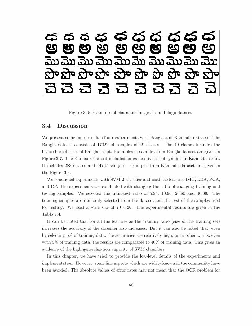
Figure 3.6: Examples of character images from Telugu dataset.

3.4 Discussion

We present some more results of our experiments with Bangla and Kannada datasets. The

Bangla dataset consists of 17022 of samples of 49 classes. The 49 classes includes the

basic character set of Bangla script. Examples of samples from Bangla dataset are given in

Figure 3.7. The Kannada dataset included an exhaustive set of symbols in Kannada script.

It includes 283 classes and 74767 samples. Examples from Kannada dataset are given in

the Figure 3.8.

We conducted experiments with SVM-2 classifier and used the features IMG, LDA, PCA,

and RP. The experiments are conducted with changing the ratio of changing training and

testing samples. We selected the train-test ratio of 5:95, 10:90, 20:80 and 40:60. The

training samples are randomly selected from the dataset and the rest of the samples used

for testing. We used a scale size of 20 × 20. The experimental results are given in the

Table 3.4.

It can be noted that for all the features as the training ratio (size of the training set)

increases the accuracy of the classifier also increases. But it can also be noted that, even

by selecting 5% of training data, the accuracies are relatively high, or in other words, even

with 5% of training data, the results are comparable to 40% of training data. This gives an

evidence of the high generalization capacity of SVM classifiers.

In this chapter, we have tried to provide the low-level details of the experiments and

implementation. However, some fine aspects which are widely known in the community have

been avoided. The absolute values of error rates may not mean that the OCR problem for

60

Feature Telugu English

20× 20 40× 40 20× 20 40 × 40

CM 20.78 12.32 7.25 6.48

ZM 8.45 5.48 2.04 1.12

DCT 9.67 2.71 2.14 1.04

DFT 15.71 6.71 5.37 3.31

PCA 4.62 2.93 0.86 0.46

LDA 2.56 1.67 0.29 0.23

RP 2.49 1.66 0.28 0.23

DT 3.48 3.17 0.98 0.87

IMG 3.18 2.84 0.28 0.23

Table 3.4: Experiments on various scripts, with SVM-2.

Figure 3.7: Examples of character images from Bangla dataset.

these scripts can expect these performances. These rates are obtained on isolated segmented

characters. To improve the accuracies beyond whatever we have reported here, one may

have to tune the parameters, fuse the features and employ better image processing and

segmentation algorithms. That is not the objective of this work.

The cost we need to pay for a richer feature space is the additional computations in

pattern classification. An alternate way of achieving this is using kernels as in SVM. Our

experience is that, one can obtain very high classification rates and efficient classification

61

Figure 3.8: Examples of character images from Kannada dataset.

Language # Classes # Samples Feat Dim. Train:Test Ratio

5:95 10:90 20:80 40:60

Bangla 49 17022

IMG 400 95.99 97.00 97.45 97.83

PCA 350 95.78 96.84 97.41 97.66

LDA 350 96.26 97.01 97.43 97.66

RP 350 96.08 97.01 97.44 97.66

Kannada 283 74767

IMG 400 96.60 97.76 98.23 98.67

PCA 350 96.21 97.63 98.17 98.59

LDA 350 96.47 97.69 98.24 98.62

RP 350 96.40 97.66 98.20 98.63

Table 3.5: Experiments with Bangla and Kannada datasets.

on our state of the art desktop computers.

3.5 Summary

In this chapter, we present the results of our empirical study on character classification prob-

lem focusing on Indian scripts. The dimensions of the study included performance of classi-

fiers using different features, scalability of classifiers, sensitivity of features on degradation,

generalization across fonts and applicability across five scripts etc. We have demonstrated

that with a rich feature space, the problem is solvable with an acceptable performance using

state of the art classifiers like SVMs.

62

Some of the interesting results of our experiments are summarized below. SVM classifiers

are found to outperform other classifiers throughout the experiments. The naive Bayes and

decision tree classifiers are the poorly performing ones. Statistical features with a rich

feature space performed well across the classifiers. A large feature space derived with the

statistical feature extraction schemes, and a classifier with high generalization capability

are found to be the ideal candidates for solving character classification problems in Indian

languages.

63

Chapter 4

Design and Efficient

Implementation of Classifiers for

Large Class Problems

4.1 Introduction

Multiclass pattern classifiers have significant applications in many real-life problems. Tra-

ditional pattern recognition literature aims at designing optimal classifiers for two class

classification problems [2]. However, most of the practical problems are multi-class in na-

ture. When the number of classes increase, problem becomes challenging, both conceptually

as well as computationally. Large class classification problems often appear in object recog-

nition, bio-informatics, character recognition, biometrics, data-mining etc.

The analysis of scalability of classifiers presented in Subsection 3.3.3, shows that many of

the popular classifiers fail to scale to large number of classes. Our study reveal that classifier

systems with multiple modular classifiers scale well. Our empirical studies and theoretical

results provide convincing evidences to support the utility of SVM (multiple pair-wise)

classifiers for solving the problem. In addition to this, recent comparative studies have

argued that Support Vector Machine (SVM) based classifiers provide the best results on a

wide variety of data sets [60, 39].

However, a direct use of multiple SVM classifiers has certain disadvantages. One of

the disadvantage comes in terms of storage and computational requirements. SVMs were

originally designed for binary (two-class) classification [61]. Direct extension of SVM to

multiclass classification is not attractive due to the complexity of the associated optimization

64

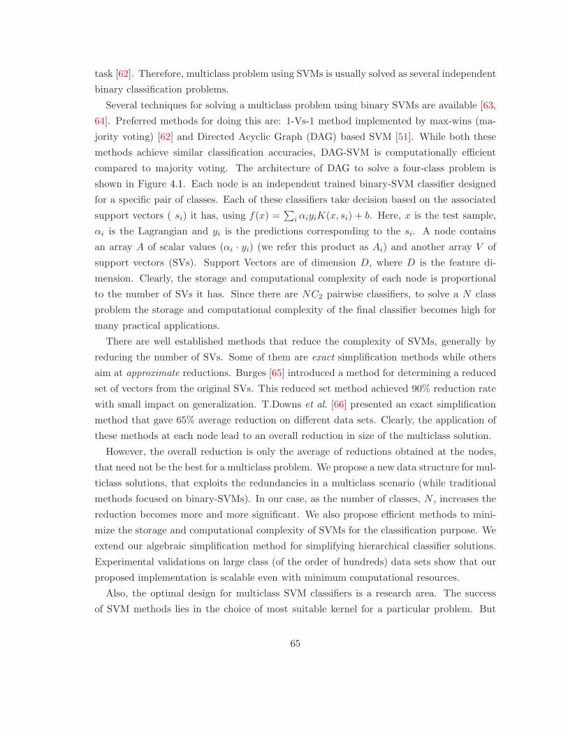
task [62]. Therefore, multiclass problem using SVMs is usually solved as several independent

binary classification problems.

Several techniques for solving a multiclass problem using binary SVMs are available [63,

64]. Preferred methods for doing this are: 1-Vs-1 method implemented by max-wins (ma-

jority voting) [62] and Directed Acyclic Graph (DAG) based SVM [51]. While both these

methods achieve similar classification accuracies, DAG-SVM is computationally efficient

compared to majority voting. The architecture of DAG to solve a four-class problem is

shown in Figure 4.1. Each node is an independent trained binary-SVM classifier designed

for a specific pair of classes. Each of these classifiers take decision based on the associated

support vectors ( si) it has, using f(x) =∑

i αiyiK(x, si) + b. Here, x is the test sample,

αi is the Lagrangian and yi is the predictions corresponding to the si. A node contains

an array A of scalar values (αi · yi) (we refer this product as Ai) and another array V of

support vectors (SVs). Support Vectors are of dimension D, where D is the feature di-

mension. Clearly, the storage and computational complexity of each node is proportional

to the number of SVs it has. Since there are NC2 pairwise classifiers, to solve a N class

problem the storage and computational complexity of the final classifier becomes high for

many practical applications.

There are well established methods that reduce the complexity of SVMs, generally by

reducing the number of SVs. Some of them are exact simplification methods while others

aim at approximate reductions. Burges [65] introduced a method for determining a reduced

set of vectors from the original SVs. This reduced set method achieved 90% reduction rate

with small impact on generalization. T.Downs et al. [66] presented an exact simplification

method that gave 65% average reduction on different data sets. Clearly, the application of

these methods at each node lead to an overall reduction in size of the multiclass solution.

However, the overall reduction is only the average of reductions obtained at the nodes,

that need not be the best for a multiclass problem. We propose a new data structure for mul-

ticlass solutions, that exploits the redundancies in a multiclass scenario (while traditional

methods focused on binary-SVMs). In our case, as the number of classes, N , increases the

reduction becomes more and more significant. We also propose efficient methods to mini-

mize the storage and computational complexity of SVMs for the classification purpose. We

extend our algebraic simplification method for simplifying hierarchical classifier solutions.

Experimental validations on large class (of the order of hundreds) data sets show that our

proposed implementation is scalable even with minimum computational resources.

Also, the optimal design for multiclass SVM classifiers is a research area. The success

of SVM methods lies in the choice of most suitable kernel for a particular problem. But

65

there is no pre-designed method to find the best kernel for a problem. We address these

issues by efficiently designing a Decision Directed Acyclic Graph (DDAG) classifier with

SVM pair-wise classifiers as nodes in the graph. We argue that, in a large class problem

most of the pairs of classes are linearly separable. Therefore, we choose linear kernel for the

pair-wise SVMs in the DDAG.

In the Section 4.2 we discussed the use of a multiclass data structure which is best suited

to store the support vectors(SVs) for large class problems. In the Section 4.3 we propose

an algebraic solution to reduce the number of support vectors in a hierarchical manner. In

this thesis we have given more attention to the classification module present in the OCR

architecture. In the Section 4.4, we discuss about the character classification scheme used

for designing the OCR system.

4.2 Multiclass Data Structure(MDS)

In this section, we introduce our Multiclass data structure (MDS) for efficiently storing and

accessing SVs. MDS for a N -class problem is shown in Figure 4.2. It consists of two major

components. First one is a set of nodes, each of which represents a modified IPI node. (IPI

(Independent Pairwise Implementation) represents the nodes in a naive implementation.)

Second one is a list of vectors L, containing reduced set of SVs for the multiclass problem.

The effectiveness of our solution basically comes from the following change in the node

structure. The first scalar array A in the node is retained as such, while the second array of

vectors that stored the SVs in the original node (Figure 4.1) are replaced with a scalar array

INDEX in MDS. This second array now stores the index positions of the corresponding

SVs, that are moved to list L.

IPI ideally treats the set of SVs that belong to a particular binary classifier to be in-

dependent of SVs that belong to other binary classifiers. Hence it stores the SVs of each

binary classifier at the corresponding node. MDS breaks the independence assumption and

maintains a single list (L) of all SVs, thereby allowing component binary classifiers to point

a single instance of the shared SVs. Thus it brings a true and exact multiclass reduction,

exploiting the redundancies in a multiclass scenario. This helps in scaling the solution for

large classes as explained below.

Table 4.1 summarizes the analysis of space required by IPI and MDS implementation.

Though MDS adds an extra storage (S × i) for indexing, it is negligible considering the

amount of reduction in the storage of SVs for large class problems. Our experiments show

that for a 300-class problem R is only 1% of S. As N increases, the space reduction

66

2/ 4

1/ 2 2/ 3 4/ 3

2 3 41

Not 1Not 2

Not 3Not 3

Not 4Not 2

1/ 3

Not 3 Not 2Not 4Not 1

1/ 4

Not 1Not 4

..

α . y SVs

..

a1 SV − 1a2

SV − k

SV − 2

ak

A V(a)

..

α . y SVs

..

a1a2 SV − 2

ak

A V

SV − 1

SV − k

g beca d f h

a, e, c, g Vs b, d, f, h

a, c Vs e, g b, d Vs f, h

b Vs de Vs ga Vs c f Vs h

(b)

Figure 4.1: (a)DAG with independent binary classifiers. (b) BHC architecture

Space requirement of IPI in bytes:

Storage of SVs : S ×D × d

Storage of Ai values : S × d

Total size: S ×D × d + S × d

Space requirement of MDS in bytes:

Storage of SVs : R×D × d

Storage of Ai values : S × d

Extra space for indexing : S × i

Total size: R×D × d + S × (d + i)

Table 4.1: Space complexity analysis. Let S be the total number of SVs in all the nodes in

Figure 4.1, R be the number of SVs in the list L of Figure 4.2 and D is the dimensionality

of the feature space. Also let d be sizeof(double), i be sizeof(integer).

approaches S−RS , since the space requirement of A and INDEX are negligible compared

to that of support vectors.

Though the N(N−1)2 pairwise classification problems are independent, we observe that

many of these classifiers share support vectors. This is because of the fact that SVs are

the samples on the class boundaries. Therefore, even if the number of classes increase, the

unique support vectors in the solution increase only marginally. This is the primary reason

for obtaining very high reduction in space requirement. Figure 4.3 shows that as many

binary classifiers as there are in the decomposed solution, the dependency among them will

also be high for any type of kernel. That is, the number of shared SVs is more. Hence, as

we combine the SVs of the binary classifiers into a unique reduced set, we can see that the

reduced set converges only with SVs from a fraction of binary classifiers.

67

....

..

...

...

1 Vs 2a1a2

ak

1 Vs N1

SV − 1

SV − 3SV − 2

Reduced list ofASVs(L)

SV − R

2

1

0

SV − ’R−1’

SV − ’K+1’SV − K K−1

K

R−1

R−2..R−1

KK−1

.2

.R−2

..10

K−1

Node 1

Node (N−1)

Node N(N−1)/2

INDEX

(N−1) Vs N

Figure 4.2: Multiclass data structure. Support vectors are stored in a single list (L) uniquely.

Algorithm 4 shows the computations performed by a binary SVM for classifying a sample.

To decide the class of a given test sample x, f(x) =∑

i αiyiK(x, si)+b must be computed for

the binary classifiers that fall along the evaluation path. The costly part of this computation

is the evaluation of the kernel function K(x, si) for each support vector si. So if the same

vector si is used in more than one of those binary SVMs, we compute the K(x, si) only once

and reuse it at other places. Algorithm 4 uses MDS to implement this with, KERNEL to

store K(x, si) and associated FLAG for indication.

In the proposed implementation, we need to maintain a unique list of support vectors.

This is done by incrementally inserting the non-redundant SVs into L. Though it adds

little extra time during training, there are notable benefits as well such as the number of

write and read File I/O operations is reduced from order of S to R for creating the model

file (training phase) and loading it in memory (during classification) respectively. Also the

cost of adding and accessing a SV to and from the list is constant.

We achieve significant reduction in space and testing time with minimal extra compu-

tation during the training. In the proposed implementation, we only need to maintain a

unique list of support vectors. This is done by incrementally inserting the non-redundant

SVs into L. Apart from that, the number of write and read File I/O operations is reduced

from order of S · D to R · D for creating (training phase) the model file and loading it in

memory (during classification) respectively.

There are two components to the added cost. One comes from creating the list of reduced

SVs and the second is from building the index associated with each node. The upper bound

68

0 N(N−1)/8 N(N−1)/4 3*N(N−1)/8 N(N−1)/2

Nodes−Binary SVMs

No.

of S

Vs

in r

educ

ed s

et

Linear

Polynomial

RBF

R

R/2

R/4

R

3R/4

Figure 4.3: Dependency analysis. R is the total number of SVs in the reduced set for RBF

kernel.

for the former is O(S ·R ·D) and for the later it is O(S). However, practically both the list

and the index are built online as the SVs are added – leaving the training time comparable

to DAG. Also note that the cost of adding and accessing a SV to and from the list are

constant. Apart from that, the number of write and read File I/O operations is reduced

from order of S · D to R · D for creating (training phase) the model file and loading it

in memory (during classification) respectively, ignoring the I/O cost for INDEX which is

negligible.

Algorithm 4 SVM CLASSIFY(Node, Sample)

1: for i = 1 to (Node→NumOfSVs) do

2: index ← (Node → INDEX[i])

3: if FLAG[index] = 0 then

4: KERNEL[index] ← K(Sample, L[index])

5: FLAG[index] ← 1

6: end if

7: Add KERNEL[index]× (Node→ A[i]) to D

8: end for

9: Add (Node → b) to D

10: RETURN sign of D

11: END SVM CLASSIFY

69

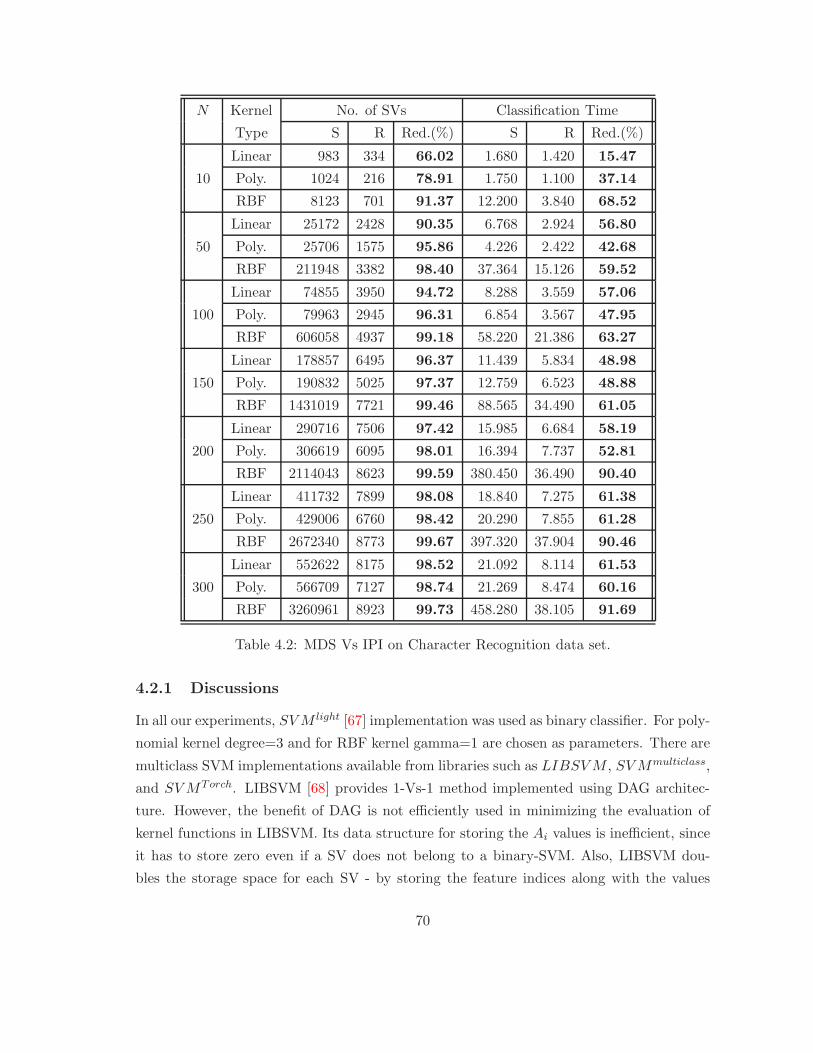
N Kernel No. of SVs Classification Time

Type S R Red.(%) S R Red.(%)

10

Linear 983 334 66.02 1.680 1.420 15.47

Poly. 1024 216 78.91 1.750 1.100 37.14

RBF 8123 701 91.37 12.200 3.840 68.52

50

Linear 25172 2428 90.35 6.768 2.924 56.80

Poly. 25706 1575 95.86 4.226 2.422 42.68

RBF 211948 3382 98.40 37.364 15.126 59.52

100

Linear 74855 3950 94.72 8.288 3.559 57.06

Poly. 79963 2945 96.31 6.854 3.567 47.95

RBF 606058 4937 99.18 58.220 21.386 63.27

150

Linear 178857 6495 96.37 11.439 5.834 48.98

Poly. 190832 5025 97.37 12.759 6.523 48.88

RBF 1431019 7721 99.46 88.565 34.490 61.05

200

Linear 290716 7506 97.42 15.985 6.684 58.19

Poly. 306619 6095 98.01 16.394 7.737 52.81

RBF 2114043 8623 99.59 380.450 36.490 90.40

250

Linear 411732 7899 98.08 18.840 7.275 61.38

Poly. 429006 6760 98.42 20.290 7.855 61.28

RBF 2672340 8773 99.67 397.320 37.904 90.46

300

Linear 552622 8175 98.52 21.092 8.114 61.53

Poly. 566709 7127 98.74 21.269 8.474 60.16

RBF 3260961 8923 99.73 458.280 38.105 91.69

Table 4.2: MDS Vs IPI on Character Recognition data set.

4.2.1 Discussions

In all our experiments, SV M light [67] implementation was used as binary classifier. For poly-

nomial kernel degree=3 and for RBF kernel gamma=1 are chosen as parameters. There are

multiclass SVM implementations available from libraries such as LIBSV M , SV Mmulticlass,

and SV MTorch. LIBSVM [68] provides 1-Vs-1 method implemented using DAG architec-

ture. However, the benefit of DAG is not efficiently used in minimizing the evaluation of

kernel functions in LIBSVM. Its data structure for storing the Ai values is inefficient, since

it has to store zero even if a SV does not belong to a binary-SVM. Also, LIBSVM dou-

bles the storage space for each SV - by storing the feature indices along with the values

70

(though it could help in case the SVs are highly sparse). While these implementations are

concerned about relatively simple multiclass problems (20 or 30-classes), we worry about

problems with hundreds of classes.

SV M light computes a single linear weight vector w =∑

i αiyisi for linearly separable

problems. So the binary classifier stores only w and need not require the SVs for classifica-

tion. Therefore the multiclass solution stores only N(N−1)2 linear weights and uses (N − 1)

of them for classifying a sample. Though this linear weight method gives better space

reduction for 10 and 50-class problems, MDS has better reduction for large classes, since

R < N ·(N−1)2 for N >= 100 in Table 4.2. However, R > (N − 1) for all N = 10 · · · 300,

hence linear weight method has faster classification rate always. (The serious limitation of

the linear weight method is that it is not applicable to non-linear kernels). We conducted

our experiments were on UCI data sets [41] and our own Indian language OCR data sets.

In our experiments, we report the number of SVs that were found in IPI (S) and compare

it with the number of reduced SVs (R) obtained using MDS implementation. We also report

the reduction in average classification time (per sample in milliseconds) that is obtained

by reusing the computation of K(x, si). The accuracy in all our experiments is preserved

exactly.

Table 4.3 shows the results against two UCI data sets. The reduction in SVs for linear and

polynomial kernels are observed to be closer, while RBF kernel gives higher reduction rate.

Because RBF solution picks more samples as SVs in IPI, that leads to more redundancy

among the SVs from the binary solutions. Also, comparing the results from PenDigits and

Letters data sets shows that the reduction rate increases with increase in number of classes,

irrespective of the type of kernel used.

Experiments with large class character recognition data sets were performed to test the

scalability of our proposed implementation. A few examples from the dataset are shown in

the Figure 4.4. The results are shown in Table 4.2 for different number of classes N , with

100 samples per class for training. We obtain a maximum of around 98.5% of reduction

in SVs and 60% reduction in classification time for linear and polynomial kernels on the

300-class data set. The time reduction is lesser than the reduction in SVs obtained, since

classifying a sample involves only N − 1 binary classifiers and not all the N ·(N−1)2 .

As one can see, the reduction in SVs gradually increases as N goes from 10 to 300. The

reduction rate in classification time also shows similar increment except on RBF kernel

for N >= 200. The reason for the sharp increase in the exceptional cases comes from S

being very large, hence the classifier model (having the SVs) does not fit into main memory

space (on a 2GB machine). We found that the virtual memory swap space was used, that

71

Figure 4.4: Sample characters from the recognition dataset. These are characters present

in Malayalam script.

made the classification process slower in IPI. However, MDS implementation exploits the

redundancy among these SVs, thereby giving a reduced set of SVs R with more than 99%

reduction. Thus the model file in MDS no more requires the swap space. This observation

clearly shows that the MDS implementation is scalable for large class problems even if the

available resources are less.

Data set Kernel No. of SVs

Name Type IPI(S) MDS(R) Red.(%)

PenDigitsLinear 5788 2771 52.13

Poly. 3528 1777 49.63

(10-class) RBF 67450 7494 88.89

LettersLinear 113249 15198 86.58

Poly. 80553 12961 83.91

(26-class) RBF 482975 18666 96.14

Table 4.3: MDS Vs IPI on UCI data sets.

4.2.2 SVM simplification with linear kernel

When we know that our data is linearly separable in the input space, the kernel mapping

- K(x, si) is simply the dot product x.si. Hence we can compute and store single vector

w =∑r

i=1 αiyisi. Therefore the decision surface becomes f(x) = x.w + b. That is, the

binary classifier replaces a set of SVs with a single linear weight vector(w) of dimension D.

Thus it saves both storage space and classification time.

72

For a N − class problem using above simplification, we need to store only N (̇N − 1)/2

linear weight vectors. And for classifying a sample vector (x), (N−1) vector inner-products

needs to be calculated using DAG. However the above simplification is not applicable for

non-separable problems, where we need to apply non-linear kernel mapping to feature space

in which the problem becomes linearly separable. (Also replacing the support vectors is

against the philosophy of SVM).

No. of Size of Lin. Size of Reduced Reduction

Classes Wt.s File SV File in Size(%)

10 156K 1.1M -85.81

50 4.0M 7.8M -48.71

100 16M 14M 12.50

150 36M 23M 36.11

200 64M 27M 57.81

250 99M 30M 69.69

300 143M 33M 76.92

Table 4.4: Linear weights Vs MDS on OCR data-sets

The results of the model file size the file with MDS and the one using linear weight

are compared in Table 4.4. Though for 10-class and 50-class, we get negative reduction in

the size of the model file with MDS; It performs better than linear weights when N ·(N−1)2

becomes larger than R (number of reduced set of SVs). But for classification, linear weights

always took lesser time in our experiments. This is because we can observe from Table

4.2, that R > (N − 1) for linear kernels for all N (but remember that linear weight is not

applicable to other kernels).

4.3 Hierarchical Simplification of SVs

Downs et al. [66] introduced a method called Exact Simplification for recognizing and elim-

inating unnecessary SVs in SVMs. The method reduces a given set of SVs by finding those

SVs that are linearly dependent of other SVs in the feature space and removing them from

the solution. Suppose we have a support vector solution that has r SVs that determine the

decision surface

f(x) =r

∑

i=1

αiyiK(x, si) + b. (4.1)

73

Now suppose that SV xk is linearly dependent on other SVs in the feature space, i.e.,

K(x, sk) =r

∑

i=1,i6=k

ciK(x, si), where the ci are scalar constants. Then the solution can be

simplified as f(x) =r

∑

i=1,i6=k

αiyiK(x, si) + b, where αi are the updated Lagrangians that

keeps the solution otherwise unchanged.

A direct extension of this exact simplification to any hierarchical multiclass SVM solutions

is to apply the reduction method on each of the component classifiers. This reduces each

component classifier by removing a subset of SVs, leaving only the linearly independent SVs

in their corresponding solutions. However, the obtained reduction from each component

classifier need not be the best for the overall multiclass solution. At the same time, the

method cannot further eliminate any SVs since all of them are now linearly independent

within a component solution.

We can eliminate SVs further from the solutions of the component classifiers, if we break

the linear independence. This is possible if we add new vectors to each component solutions.

Suppose we have a component classifier that has a reduced set of SVs I that are linearly

independent. We could add a new set of vectors to I to get an extended set of vectors E. If

the extended set of vectors are no longer linearly independent, then we can further reduce

the component classifier by eliminating many SVs. Note that while we are eliminating a

subset of SVs from I, we have already added some new vectors to the solution to get the

benefit. The addition of new vectors is justifiable and do not bring any extra cost when we

add the SVs that belong to component classifiers that are up in the hierarchy in a decision

path to the one at a lower level for reducing the later. Since the kernel computations

K(x, si) for those SVs once computed at any component classifier higher in the decision

path are reusable anywhere down the decision path.

The hierarchical simplification involves two steps as given in Algorithm 5. The algorithm

also simplifies a multiclass solution exactly, by reducing the number of SVs as explained

below.

Suppose a component classifier X has its solution of the form Equation 4.1. Let V denote

the set of SVs in the solution. Step 1 of the algorithm reduces V to a subset I of SVs and

the solution becomes

f(x) =r

∑

i=1,si∈I

αiyiK(x, si) + b (4.2)

Step 2 of the algorithm now adds a set of SVs A that are picked up from any of the

component classifiers above X in the decision path. Let A = a1, a2, ...., ak be the SVs with

74

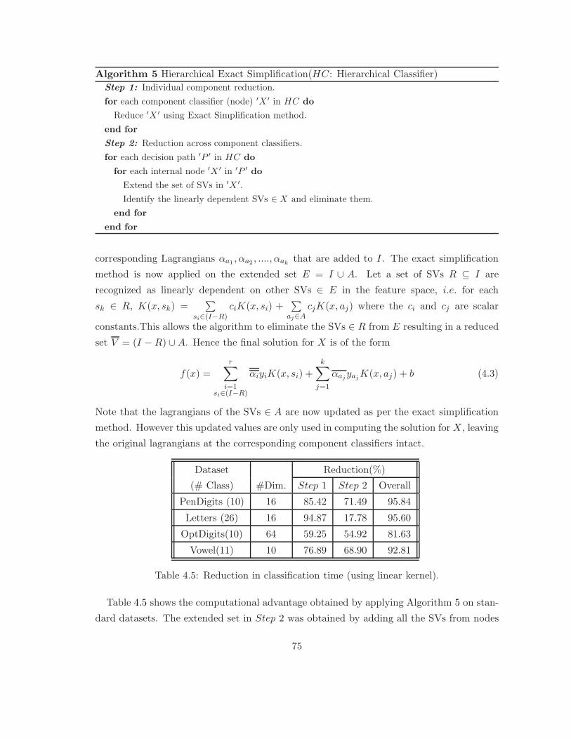
Algorithm 5 Hierarchical Exact Simplification(HC: Hierarchical Classifier)

Step 1: Individual component reduction.

for each component classifier (node) ′X ′ in HC do

Reduce ′X ′ using Exact Simplification method.

end for

Step 2: Reduction across component classifiers.

for each decision path ′P ′ in HC do

for each internal node ′X ′ in ′P ′ do

Extend the set of SVs in ′X ′.

Identify the linearly dependent SVs ∈ X and eliminate them.

end for

end for

corresponding Lagrangians αa1, αa2

, ...., αakthat are added to I. The exact simplification

method is now applied on the extended set E = I ∪ A. Let a set of SVs R ⊆ I are

recognized as linearly dependent on other SVs ∈ E in the feature space, i.e. for each

sk ∈ R, K(x, sk) =∑

si∈(I−R)

ciK(x, si) +∑

aj∈AcjK(x, aj) where the ci and cj are scalar

constants.This allows the algorithm to eliminate the SVs ∈ R from E resulting in a reduced

set V = (I −R) ∪A. Hence the final solution for X is of the form

f(x) =

r∑

i=1si∈(I−R)

αiyiK(x, si) +

k∑

j=1

αajyaj

K(x, aj) + b (4.3)

Note that the lagrangians of the SVs ∈ A are now updated as per the exact simplification

method. However this updated values are only used in computing the solution for X, leaving

the original lagrangians at the corresponding component classifiers intact.

Dataset Reduction(%)

(# Class) #Dim. Step 1 Step 2 Overall

PenDigits (10) 16 85.42 71.49 95.84

Letters (26) 16 94.87 17.78 95.60

OptDigits(10) 64 59.25 54.92 81.63

Vowel(11) 10 76.89 68.90 92.81

Table 4.5: Reduction in classification time (using linear kernel).

Table 4.5 shows the computational advantage obtained by applying Algorithm 5 on stan-

dard datasets. The extended set in Step 2 was obtained by adding all the SVs from nodes

75

that are higher in a decision path to a particular node to reduce the later and the procedure

was repeated iteratively. Note that the computational advantage comes with an additional

storage requirement of modified Lagrangian values. The reductions obtained are problem

dependent in both the steps as also observed by Downs et al. [66] in their experiments.

4.4 OCR and Classification

In this section we are explaining the classification scheme used in the design of our OCR.

Figure 4.5 shows the basic architecture of an optical character recognition system. A more

detailed figure is given in Chapter 1 (Refer Figure 1.1). In this work we have given attention

to the classification module. Here we explain the design and implementation details of the

classification scheme used for our OCR.

Post−processing

SegmentationPre−processingFeature

Extraction

ClassificationUnicode(Text)

Document Image

Figure 4.5: Basic architecture of an OCR system. In this work we have given attention to

classification module.

The design approach to classifiers can be based on two different philosophies. The first

one uses complex classifier models such as neural networks for direct classification of a

sample into one of the N classes possible, resulting in an efficient classifier that is trainable.

The second approach uses the divide an conquer strategy, where an ensemble of simple

binary classifiers are integrated to form the final N -class classifier. Our classifier needs to

handle a large number of classes, with close similarities between certain component pairs.

Hence we prefer the latter approach for our OCR classification, as the individual classifiers

can be independently trained and analyzed for improving the overall performance.

One could choose from a large set of classification algorithms for the binary classifiers. We

have experimented with a variety of algorithms and found that Support Vector Machines

(SVMs) offer the best performance for this problem in most cases. It’s success comes out of

its capability to maximize the margin and thereby enhancing the generalization in classifier

design. Thus SVM differs from the neural network based approaches which, in a way,

76

maximizes the empirical accuracy rates measured on the training data. SVMs, built on

statistical learning theory, maximizes the generalization and hence shown superior results.

The objective function which SVM minimizes is convex and there by guaranteeing a global

minima (unlike Neural network based approaches, which often gets trapped in local minima)

with a set of additional constraints. Final solution to the classification is expressed in terms

of some of the training samples (support vectors) and the decision rule is expressed in terms

of dot products of inputs with support vectors. This helps in using the kernel methods and

deriving nonlinear decision boundaries.

However, in this work, we decided to explicitly increase the feature dimensions (mildly)

and make the data more separable for pairwise classification and thereby to avoid the

floating point operations required for kernel. This makes the computations efficient. Far

more than that, this allow a compact representation of the decision boundary. Thus our

final SVM classifier stores the decision boundaries directly rather than storing the support

vectors as in most popular implementations. This makes our SVM classifier, memory and

time efficient compared to the popular implementations.

DDAG is SVM’s one of the fastest combination strategies for multiclass classification [51].

In DDAG the modular classifiers are arranged in a hierarchical manner. The advantages of

hierarchical modular classifiers are :

1. Simpler classifiers compared to multiclass methods.

2. Uses lesser space compared to other ensemble methods.

3. Highly flexible because of its modularity, and hence node level training is possible.

4. Approach is scalable to large class problems.

All the N ·(N−1)2 pair-wise classifiers are combined in a DDAG to create the classification

module in the OCR architecture. Figure 4.6 shows the DAG architecture for the Malayalam

OCR design. We have considered 205 classes/symbols in this design.

Given an input sample x for classification, it is first presented to the root node of the

DDAG for decision. The decision that happens at each node of the classifiers is not which

class the sample belongs to, but which class the sample does not belongs to. One of the

classes is rejected as a feasible class at the root node and the sample thus reach the root

node of the left or right sub-DAG, which does not contain the rejected class. Another

class rejection takes place at this root and the sample follows an edge leading to one of the

sub-DAGs of the current root node. This way, the sample rejects N − 1 classes before it

reaches the leaf node of the DAG. The sample x is assigned the label corresponding to the

77

.. .

.

.

.

.

.

.

.

.

.

input image

Figure 4.6: DDAG architecture for Malayalam OCR.

leaf node it reached. It can be observed that the number of binary classifiers built for a N

class classification problem is N ·(N−1)2 . The DDAG design for Malayalam OCR contains a

total of 20910(205∗204/2) nodes. However, for each test case only 204 nodes are evaluated.

4.5 Summary

In this chapter we have presented an efficient data structure for implementing multiclass

solutions. This data structure is applicable to any multiclass classification technique that

builds the solution on binary SVMs. We had shown that our data structure reduces both

space and time complexity significantly on multiclass problems. We are presently exploring

algebraic reduction schemes on the list L. We also explained the design strategies used for

classification module in our OCR design. The experimental results and the performance

evaluation of the OCR system is discussed in the next chapter.

78

79

Chapter 5

Performance Evaluation

5.1 Introduction

We have conducted extensive experiments to validate the OCR modules and overall perfor-

mance on the corpus pages (mentioned in Section 2.8). This chapter provides some of our

conclusions and observations based on these experiment. For measuring the performance

of the OCR, we have taken measures like (i) Accuracy, (ii) Edit distance between two UNI-

CODE strings (iii) Substitution errors, which provide a more factual distance in the case of

Indian scripts.

We use the edit distance based performance metric for the evaluation of document image

recognition. The same metric is used to evaluate, the accuracies at different levels such as,

symbol level, Unicode level, Akshara level, word level and Page level. Different levels of

these analysis gives different aspects of OCR. Refer Section 2.5 for the definition of symbol,

Unicode and Akshara.

The lowest level is symbol level edit distance. This gives direct information about the

number of symbols misclassified. Symbols are the base for the classifier design. Therefore,

accuracy calculated at the symbol level gives direct information about the strength and

generalization capacity of a classifier. The confusion matrix obtained by symbol level anno-

tation, misclassifications occurred during classification. This is a very valuable information

to redesign the classifier. The modular classifiers can be retrained to get better classification

accuracy.

The next level of performance metric is Unicode level. Once the classifier classifies all the

symbols, the class labels have to be converted to the corresponding Unicode. As we have

explained in chapter 2, the isolated symbols may or may not be a meaningful character.

80

Sometimes, a Unicode might be composed of more than one symbol. On the other hand,

there will be more than one Unicode corresponding to one symbol. The second case is

more popular. Examples of this type is a huge set of composite/conjunct characters. When

we measure the Unicode level accuracy, it is important to reorder the symbol labels in a

meaningful manner. This is important because of the fact that, the symbols in the text may

or may not occur in the order it has to be represented in Unicode. Therefore, compared to

the total number of symbols the the total number of Unicode is usually higher in a document

page of Indian languages. The major change in the representation of Unicode and symbols

are the places of occurrence of matras. In symbol representation, matras may come before,

after, on top, or bottom of a character. But in Unicode representation there is a unique

way of representing matras. In Unicode, matras come after the consonant character. In

this way, the Unicode level performance metric covers, the classification errors and the

reordering errors in the OCR. This measure is generally higher than the symbol level edit

distance.

Next level of performance metric is Akshara level edit distance. An Akshara is the

basic unit of a language. An Akshara can be composed of multiple symbols or multiple

Unicodes. This metric is important from a linguistic point of view. In a document page,

the total number of Aksharas will be much lesser compared to the total number of symbols

or Unicode. This is because, the matras will not be counted as a part of the character to

which it is attached. Akshara level edit distance gives a combined measure of error caused

by mis-classification and reordering. The Akshara level edit distance is a more meaningful

error metric compared to Unicode. As our basic unit is an Akshara, this measure of error

gives a higher value of error compared to symbol and Unicode level results.

The next level of performance metric is word level. The word level error is calculated as,

total number of words with at least one error in the word to total number of words. The

word level accuracy depends on the length of the word. In this case, Languages with small

words have advantage over the languages with average word length higher. In addition to

the misclassification and reordering errors, the word level and the line level segmentation

errors will be reflected in this measure.

We have considered page level error as the highest level of error metric. This is the

average error across the pages in a book.

5.1.1 Performance Metrics

Many different metrics can be used for evaluation of OCR output. Any evaluation requires

comparison of the OCR output with annotation. Results presented in the following section

81

calculates error in terms of Edit distance. Edit distance between two strings can be com-

puted with the help of Dynamic programming. Our approach for evaluation is as explained

below. A true word sequence in the annotated corpus correspond to the Unicode sequence

C =< C1, C2, C3...Cn >. Correspondingly, OCR systems output Unicode sequence is given

by O =< O1, O2, O3...On >. We can define character error rate (CER) in the following

way:

CER =CharEditDistance(C,O)

|C|(5.1)

We could also use substitution error in place of edit distance. Number of substitutions

can be calculated by analyzing the optimal alignment path by backtracking the Dynamic

programming cost matrix. Symbol level evaluation is done using a similar approach on class

Ids or Unique Symbol Identifiers. Language specific annotation at sub-word level is used for

achieving this. Also word level statistics are computed by considering the word boundaries

available in the annotated data.

To compare the output of our OCR with the text in the corpus, we first concatenate

all the lines in a page to get a long string. Thus we get two long strings, one the re-

sult of our OCR, and the other from the corpus. Now we dynamically compare both the

strings. Concatenation of all the lines in a page is necessary to eliminate the error when

line segmentation error (over segmentation or under-segmentation of lines) is present.

5.2 Experiments and Results

5.2.1 Symbol and Unicode level Results

The results of symbol and Unicode level error rates on various books are given in the

Table 5.1. Symbol level error is calculated on symbols which are recognizable. That is, we

have eliminated not included the symbols with cuts/ merges in this calculation. As we have

already discussed in the previous section symbol level accuracy gives an exact measure of

strength of the classifier.

Symbol Error Rate =No. of Misclassified and Recognizable Symbols

Total No. of Recognizable Symbols(5.2)

But in the Unicode results is an overall result on the book. In other words, this error

include the error caused by cuts and merges also. As the final output of the OCR system

has to be in Unicode format, it is important to have an error metric at Unicode level.

82

Unicode Error Rate =No. of Misclassified Unicode

Total No. of Unicode(5.3)

S.No Book NameSymbols Unicode

# Total Error.(%) # Total Error.(%)

1. Indulekha 321470 1.70849 423884 4.806982. ValmikiRamayanam 228188 0.94001 293822 2.827323. Sarada 235791 2.76384 299056 3.922754. Sanjayan 28661 3.34585 35668 4.597095. Hitlerude Athmakadha 125658 1.23403 163863 2.950656. BhagatSingh 458016 3.11732 489534 6.398247. Ramarajabahadoor 216744 2.12732 268653 4.387688. Thiruttu 117403 3.88202 143582 5.718329. Dharmaraja 897449 2.35065 947419 5.82614

10. IniNjanUrangatte 277257 1.71141 315259 3.7457611. ViddhikaluteSwargam 62396 3.34805 74719 6.8986812. Janmadinam 86269 2.41994 108881 4.98745

Table 5.1: Symbol level and Unicode level error rates on Malayalam books.

Now we analyze the Unicode and Symbol level results based on the cuts, merges and other

distortion for the book Indulekha. Table 5.2 shows the cuts, merges, and other noise details

of the book Indulekha. We can notice that the sum of cuts, merges, noise and symbol level

classification error comes out to be 4.179951, and the total Unicode level error is 4.80698.

These numbers almost matches, but the Unicode level error rate is a bit higher than the

total error rate calculated from the results. This increase in the error rate at Unicode level

is due to the fact that, one symbol level misclassification may results in more than one

Unicode level error. This happens when a conjunct character get misclassified. There are

some rare occasions where the reverse effect happens. That is one Unicode error constitute

to more than one symbol error. But these scenario occurs rarely compared to the occurrence

of conjunct characters in the language. Thus the Unicode error will be always higher than

the symbol level results.

When a conjunct character got misclassified, we count one error in the symbol level.

But a set of different scenarios can happen. Consider a conjunct character which has 3

components. Mostly it is composed of a basic character + a halant another basic character.

If this conjunct character got misclassified to another entirely different conjunct character

character, it contributes two errors in Unicode. In this case, both the base characters are

wrong and only the middle halant is correct. Another scenario, the first or second base

character is correct, only one of them got wrong. This will contribute, one error in Unicode.

Yet another situation is a conjunct character getting misclassified to a base character.

83

Name of the Book IndulekhaTotal No. of Symbols 321470Total No. of Unicode 423884Symbol level classification error 1.70849Cuts 1.57091Merges 0.45852Noise 0.44203Total (Cut, Merge, Noise & Misclassification ) 4.17995Unicode level edit distance 4.80698

Table 5.2: Symbol level and Unicode level error rates on Malayalam books.

This will contribute, one misclassification error and two delete error, a total of three edit

distance. In the above situation suppose this conjunct character misclassified to a basic

character which is one of the constituent basic characters of the same conjunct character.

This case will contribute two delete error, and thus two edit distance.

Consider a case where the reverse scenario happens, i.e., a basic character gets misclas-

sified to a conjunct character. Here, if the basic character matches with one of constituent

characters of the conjunct character this error will contribute two insert errors and thus

two edit distance. Otherwise, this will contribute one misclassification and two inserts, a

total of three edit distance.

Using the dynamic programing technique we also calculated the percentage of substitu-

tion, inserts or deletes that contributed the total edit distance for the Unicode. Table 5.3

gives the result of these experiments. These numbers gives an approximate match with the

calculation we have done already.

S.No Book Name Edit-Dist Substitution Inserts Deletes

1. Indulekha 4.80698 2.13179 2.00354 0.987612. ValmikiRamayanam 2.82732 1.49772 0.79015 0.654253. Sarada 3.92275 2.10003 1.22171 0.899114. Sanjayan 4.59709 2.31822 1.09669 1.576665. Hitlerude Athmakadha 2.95065 1.35846 0.70114 0.947036. BhagatSingh 6.39824 3.94839 3.18630 1.193157. Ramarajabahadoor 4.38768 2.57491 1.95001 0.800748. Thiruttu 5.71832 4.92912 2.53587 1.263419. Dharmaraja 5.82614 1.43978 1.68051 1.30065

10. IniNjanUrangatte 3.74576 1.89763 0.75756 1.1975911. ViddhikaluteSwargam 6.89868 2.45957 1.29882 2.7575512. Janmadinam 4.98745 1.80187 0.82338 2.24626

Table 5.3: Unicode level error rates classified to errors due to substitution, inserts and deletes, onMalayalam books scanned with 600dpi resolution.

84

Table 5.4 gives the results of the same set of experiments conducted on Malayalam books

scanned with 300dpi resolution. There are slight change in the results obtained from those

with 600dpi images. These difference arises from various stages of OCR. The changes in

degradation is caused by the pre-processing stages.

S.No Book Name Edit-Dist Substitution Inserts Deletes

1. Indulekha 5.49112 2.76686 1.65368 1.070582. ValmikiRamayanam 2.23806 1.06743 0.71968 0.450953. Sarada 4.36719 2.49340 1.10736 0.766344. Sanjayan 4.31030 2.15515 1.09428 1.060875. Hitlerude Athmakadha 3.08706 1.49422 0.75763 0.835206. BhagatSingh 8.07345 4.00433 2.86220 1.206927. Ramarajabahadoor 5.43921 2.60320 1.95734 0.878668. Thiruttu 6.36529 3.27384 1.95957 1.131899. Dharmaraja 6.41670 3.05483 1.63581 1.72606

10. IniNjanUrangatte 3.75548 2.02939 0.62600 1.1000911. ViddhikaluteSwargam 5.59839 2.37324 0.94056 2.2845812. Janmadinam 4.20989 1.95101 0.69517 1.56370

Table 5.4: Unicode level error rates classified to errors due to substitution, inserts and Deletes, onMalayalam books scanned with 300dpi resolution.

5.2.2 Word level Results

The word level accuracy details of the books are given in the Table 5.5. The word level

accuracy of a book is calculated using the following formula:

Word level Accuracy =No. of Correct Words

Total No. of Words(5.4)

If all the Unicode in a word are correctly classified and correctly ordered, then that word

is considered as a correct word. To know the effect of degradations in word level accuracy

we have calculated the word accuracy in recognizable words using the formula:

Word level Accuracy =No. of Correct and Recognizable Words

Total No. of Recognizable Words(5.5)

Other than classification, many other factors effect the word level accuracy. The first

thing is, word level segmentation. There might be under-segmentation or over-segmentation

of the words. The factors that effect the segmentation errors in word level are the strength of

the segmentation algorithm, the thresholds used in the implementation of the algorithm, the

quality of printing and scanning, etc. In the case of under-segmentation, two or more words

will be segmented as a single word. This will add to the errors, even if all the symbols in

85

S.No Book NameWords

# Total (%) Accuracy # Recognizable (%) Accuracy

1 Indulekha 46281 80.7091 39644 94.22112 ValmikiRamayanam 31360 90.3000 29339 94.22003 Sarada 32897 72.1008 26671 88.93184 Sanjayan 4079 70.6301 3224 89.3615 Hitlerude Athmakadha 16403 81.3205 14291 93.33856 BhagatSingh 57252 51.3291 35246 80.12537 Ramarajabahadoor 81021 53.8404 52047 83.81278 Thiruttu 15654 59.7419 10553 88.61939 Dharmaraja 95931 51.8310 65427 86.5825

10 IniNjanUrangatte 39785 81.8273 34822 93.489711 ViddhikaluteSwargam 8793 63.1866 6435 86.340312 Janmadinam 12112 77.2705 10326 90.6353

Table 5.5: Word level results computed on all the words (degraded and non-degraded) and non-degraded words in Malayalam books.

those words have been classified correctly. On the other hand, over-segmentation segments

out a single word into multiple words. In our calculation we are adding only one error in this

case. Another thing that effects the word level accuracy is the wrong ordering of the Unicode

after classification. The importance of ordering of the components, in the case of Indian

languages, is described previously. Incorrect grammar rules used in the implementation or

printing cause a disaster in this case.

The definition of a correct word is, the word with all the Unicode are correctly classified.

If at least one of these Unicode is incorrect, that word is considered as an erroneous one.

To study the pattern of errors in the word error distribution, we studied the number of

errors in the words. The results are presented in the Table 5.6. Note that a considerable

percentage of the word error is caused by a single error in a word. In the book Indulekha,

out of 19.29% of word error, 6.9% errors are caused by words with single error, and 4.69%

of error caused by words with 2 errors.

This study opens the possibility of language models based post-processing. For example

using Unigram and Bigram models it may be possible to correct a word with a single error,

if we could identify the correct location of the error in the word.

5.2.3 Page level Results

The average page level error rates of a book is calculated using the formula:

Average Page Error Rate =

∑

Error Rates in all the Pages

Total No. of Pages(5.6)

86

S.No Book Name Total Words(%) Words with

0 Error 1 Error 2 Errors

1 Indulekha 46281 19.2909 6.90564 4.695232 ValmikiRamayanam 31360 9.7000 2.71365 4.129463 Sarada 32897 27.8992 9.17713 7.754514 Sanjayan 4079 29.3699 6.47217 9.708265 Hitlerude Athmakadha 16403 18.6795 8.90691 5.352686 BhagatSingh 57252 48.6709 12.4278 13.46207 Ramarajabahadoor 81021 46.1596 8.39412 13.12388 Thiruttu 15654 40.2581 4.22895 16.60929 Dharmaraja 95931 48.1690 13.1679 14.9682

10 IniNjanUrangatte 39785 18.1727 6.11788 6.3315311 ViddhikaluteSwargam 8793 36.8134 8.43853 6.9600812 Janmadinam 12112 22.7295 8.99934 5.30053

Table 5.6: Words with one and two errors and non-degraded words in Malayalam books.

We studied the results on the distribution of errors across pages. This is presented in

Table 5.7. This table describes the percentage of pages with different error rates. This

provides an objective method to quantitatively label the quality of the pages. Similar

studies were also conducted to know the error rates of words with one or more errors.

S.No Book NameTotal Error (%) Pages with ErrorPages Rate ( ≤ 2%) (2− 5%) (5− 10%) ( > 10%)

1. Indulekha 235 4.80 0.42 70.63 26.38 2.552. ValmikiRamayanam 170 2.82 31.76 57.64 4.11 6.473. Sarada 155 3.92 6.41 75.00 14.74 3.204. Sanjayan 35 4.59 5.55 55.55 30.55 5.555. Hitlerude Athmakadha 86 2.94 3.44 89.65 2.29 3.446. BhagatSingh 282 7.39 0 29.92 52.46 16.907. Ramarajabahadoor 141 4.38 7.80 68.79 20.56 2.838. Thiruttu 86 5.71 2.32 52.32 30.23 15.119. Dharmaraja 419 5.85 0.23 56.53 33.96 8.78

10. IniNjanUrangatte 162 3.74 4.61 66.15 11.28 1.0211. ViddhikaluteSwargam 68 6.73 0 33.33 57.97 7.2412. Janmadinam 93 4.97 0 69.89 20.43 9.67

Table 5.7: Page level accuracies and Unicode level error distribution across pages.

5.2.4 Comparison with Nayana

We compare our results with that of Nayana, a Malayalam OCR available in public. Results

on randomly selected pages from books are shown in Table 5.8. Superiority of our results

possibly comes out of the segmentation and classification algorithms. Since we do not have

87

access to the internals of the Nayana OCR, our results are superficial (black box).

Book Code No. of PagesEdit Distance Substitution

Nayana Our OCR Nayana Our OCRValmikiRamayanam 7 13.03 2.04 4.28 0.97Sanjayan 10 34.48 2.76 19.18 1.03Hitlerude Athmakadha 8 13.96 2.66 4.9 1.05BhagatSingh 6 9.72 2.63 3.97 1.31Indulekha 10 13.55 2.32 5.62 1.08Dharmaraja 9 10.33 2.52 4.19 1.31Thiruttu 10 13.44 3.91 6.17 2.11Ramarajabahadoor 10 12.19 3.02 4.05 1.41IniNjanUrangatte 9 9.49 1.91 4.23 1.02ViddhikaluteSwargam 3 13.73 4.72 4.86 1.51Janmadinam 5 15.98 3.89 5.2 1.47Tot/Ave 87 15.34 2.81 6.64 1.28

Table 5.8: Comparison with Nayana.

5.3 Quality level Results

5.3.1 Results on Scanned Quality A documents

To validate methods and implementations, we decided to scan and test the OCR on some

of the fonts and sizes. One of our observation was that the Microsoft word and fonts used

introduced too many merges in these documents and this effects the overall performance.

Since our objective was to demonstrate the symbol level accuracy and its extension to

Unicode over non-degraded pages, we minimized such word-processor/font induced errors

and did an evaluation. The experimental results are briefly summarized in Table 5.9.

Font NameFont Size

8 10 12 14E(%) S(%) E(%) S(%) E(%) S(%) E(%) S(%)

Amibili 2 0.9 1.92 0.88 2.71 0.52 4.99 0.82Karthika 2.87 1.52 0.7 0.28 1.1 0.44 0.73 0.45Lohit 3.86 1.29 2.27 1.11 2.51 1.56 3.29 1.75Nila 2.43 1.22 1.53 0.54 1.54 0.59 2.01 0.6Revathi 2.57 1.12 0.57 0.24 1.08 0.53 0.74 0.3

Table 5.9: Results on Scanned Quality A documents, in various fonts., E = Edit distance , S =Substitution error

One of our observation by testing on 5 fonts and 4 sizes (total of 20 variations) is that

our OCR extends reasonably well across these collections. However, we find that when the

88

size increases significantly, our scaling/normalization routines are not able to cope up with

it completely.

5.4 Qualitative Results/Examples

Example 1: This example (See Figure 5.1) shows a case where the recognition rate be-

come very low, because of the segmentation error at line level. In this page some of the lines

are underlined with ink. In the segmentation algorithm, we used the number of black pixels

as a threshold to detect different lines. This caused under-segmentation to those lines. So

this page gives a huge error rate of 26.84% and a substitution error of 10.85%.

Figure 5.1: A Sample Page from the book Thiruttu which has segmentation error at line

level.

89

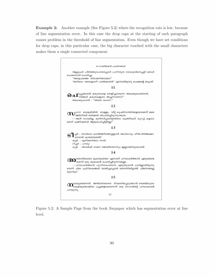
Example 2: Another example (See Figure 5.2) where the recognition rate is low, because

of line segmentation error. In this case the drop caps at the starting of each paragraph

causes problem in the threshold of line segmentation. Even though we have set conditions

for drop caps, in this particular case, the big character touched with the small characters

makes them a single connected component.

Figure 5.2: A Sample Page from the book Sanjayan which has segmentation error at line

level.

90

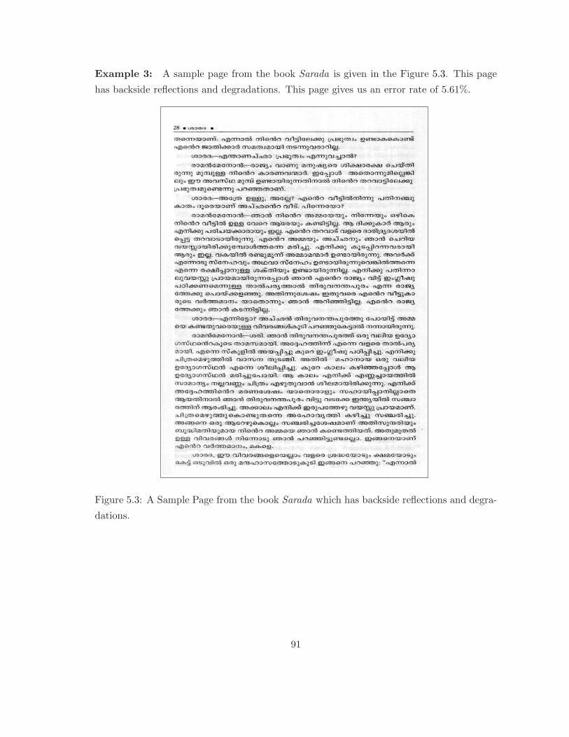
Example 3: A sample page from the book Sarada is given in the Figure 5.3. This page

has backside reflections and degradations. This page gives us an error rate of 5.61%.

Figure 5.3: A Sample Page from the book Sarada which has backside reflections and degra-

dations.

91

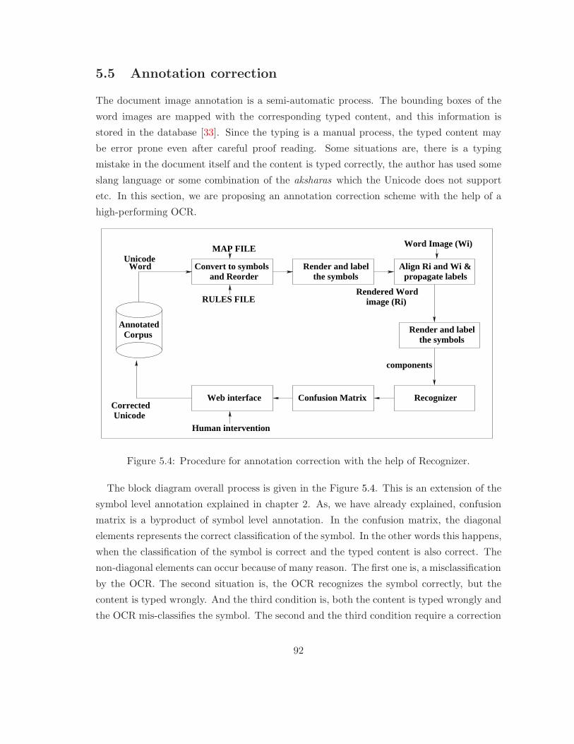
5.5 Annotation correction

The document image annotation is a semi-automatic process. The bounding boxes of the

word images are mapped with the corresponding typed content, and this information is

stored in the database [33]. Since the typing is a manual process, the typed content may

be error prone even after careful proof reading. Some situations are, there is a typing

mistake in the document itself and the content is typed correctly, the author has used some

slang language or some combination of the aksharas which the Unicode does not support

etc. In this section, we are proposing an annotation correction scheme with the help of a

high-performing OCR.

and ReorderConvert to symbols Render and label

the symbolsAlign Ri and Wi &

propagate labels

Corrected Unicode

Confusion Matrix RecognizerWeb interface

Human intervention

Annotated Corpus

WordUnicode

Render and labelthe symbols

RULES FILE

MAP FILE

Rendered Word image (Ri)

Word Image (Wi)

components

Figure 5.4: Procedure for annotation correction with the help of Recognizer.

The block diagram overall process is given in the Figure 5.4. This is an extension of the

symbol level annotation explained in chapter 2. As, we have already explained, confusion

matrix is a byproduct of symbol level annotation. In the confusion matrix, the diagonal

elements represents the correct classification of the symbol. In the other words this happens,

when the classification of the symbol is correct and the typed content is also correct. The

non-diagonal elements can occur because of many reason. The first one is, a misclassification

by the OCR. The second situation is, the OCR recognizes the symbol correctly, but the

content is typed wrongly. And the third condition is, both the content is typed wrongly and

the OCR mis-classifies the symbol. The second and the third condition require a correction

92

of the typed content in the database. We provide a web-interface to correct this data. If

the error is caused because of the first reason, we keep the content without any change.

With the help of a very high performing OCR, we can do this correction process very

fast. Consider an OCR with 95% symbol level accuracy (using the non-corrected annotated

data). In a document image of average 1000 symbols, this gives, 50 errors. In this case

we need to look at only 50 symbols instead of 1000 symbols. This way we can save 95%

of the time of annotation correction compared to a naive method, that is looking at each

symbol/word in the document image. Considering at word level, With the help of an OCR

with 60% of word level accuracy, compared to a naive process, 60% of the time can be saved.

A disadvantage of this method is, according to the above mentioned process, we are not

recognizing the symbols with cuts and merges. Thus, we are not correcting the errors that

occurred at a symbol which has a cut or a merge. To avoid the errors due to this, while

correcting the text, we can also look into the symbols with cuts or merges. Consider a

document page having with 2% cuts and 1% merge out of 1000 symbols. In this case,

With the help of an OCR with 95% of accuracy, we if add the symbols, which are cut into

multiple pieces or symbols with merges, for annotation correction, this will add up to 8 %

of symbols. That is, 80 symbols out of 1000. Still we can save 93 % of the time compared

to the naive process.

Another disadvantage of this method is, it can not detect errors, if the typed content

is wrong, and the OCR has misclassified the symbol, and the OCR output and the typed

content is same.

5.6 Summary

In this chapter we analyzed the performance of our OCR with various view points. We

used character edit distance and the substitution error as the error metrics. We conducted

experiments on real document images scanned from twelve Malayalam books, which comes

out to be more than 2000 pages. We achieved an average edit distance of 4.75 and substi-

tution error of 2.37 on these real document images, at Unicode level. We also achieved high

accuracy compared to the state of the art OCR available in public.

93

Chapter 6

Recognition of Books using

Verification and Retraining

6.1 Character Recognition

Optical character recognition (OCR) is a well researched and mature area in the litera-

ture [69, 70]. Most, if not all, of these studies focused on recognition of isolated pages or

words. With the emergence of digital libraries, in recent years, recognition of a complete

book (or a document image collection) has become important [71, 72, 73]. For machine

understanding and language processing of digitized document images, it is important to

convert them into a textual form using an OCR. We argue that the recognition of a book,

as a large collection of symbols, is considerably different from that of a word or a page.

This is due to the fact that books provide rich additional information that could be used

for improving the recognition rates of character classifiers and OCRs.

The heart of a typical OCR system is a pattern classifier, with very high performance to

recognize isolated symbols. Any error at this stage can get propagated, if not avalanched,

into the next phase. A classifier is often trained offline using labeled samples in multiple

fonts and styles. With unseen fonts/styles, the performance may deteriorate. When it

comes to the recognition of a large collection, such as a book, traditional OCRs may repeat

similar mistakes across pages. Or else an OCR designed for isolated pages need not learn

to improve the performance over time. The advantage of books from a recognition point of

view is that, books are often typeset in a single font and style. This implies that, we can

use the first few pages to obtain better performance over the rest of the collection.

We enhance the recognition/classification rates of our Book-OCR by verification and

94

retraining. New training data is introduced into the system without any manual interven-

tion. This is done with the help of a dynamic programming based verification module. We

employ an automatic learning framework to get more training samples with the help of a

verification module. Thereafter, we employ these samples to improve the performance of

the classifier by retraining. Our primary contribution is a novel procedure that is specially

suited for the recognition of books. We obtain an average performance improvement of

around 14% in classification accuracies. We obtain performance enhancement at the cost

of additional computations during the verification and retraining.

The experiments are conducted on samples from five annotated books in Malayalam

script. Malayalam is an Indian-language, which has rich literary heritage. At present there

is no robust commercial OCR system available for this language. Languages like English

employ a dictionary to correct errors in the recognition phase. However, dictionary based

post-processing techniques are not feasible for highly inflectional languages like Malayalam.

A verification scheme based on a dictionary based approach was introduced in [72]. Re-

cently, another step towards the whole book recognition is reported in [73], using mutual

entropy based model adaptation, which uses linguistic constraints to calculate the posterior

probabilities of word classes. There are also attempts to enhance the accuracy without

using an explicit language model [74] for languages where traditional post-processing is

challenging. However, they are applicable only when one simultaneously recognizes a larger

collection. In our implementation, we replace the conventional post-processor with a veri-

fication scheme.

6.2 Overview of the Book Recognizer

We present a novel and practical approach, for the recognition of symbols from a large

collection of documents. Our method employs a data-driven adaptation method to enhance

the performance, specific to a particular collection. Training the system with the samples

from the same collection to be recognized, is an obvious method to improve the performance

of the system. However, collecting the samples from the same environment and labeling

them, each time when a new book needs to be recognized, is impractical. We propose an

automatic procedure for getting labeled samples and allowing the system to adapt to the

same. This is achieved with the help of a high performance verification module, which acts

as a post-processor in the system.

The input to the recognizer is a word image. We assume that preprocessing and segmen-

tation of document images up to word level is available. The overall working of the system

95

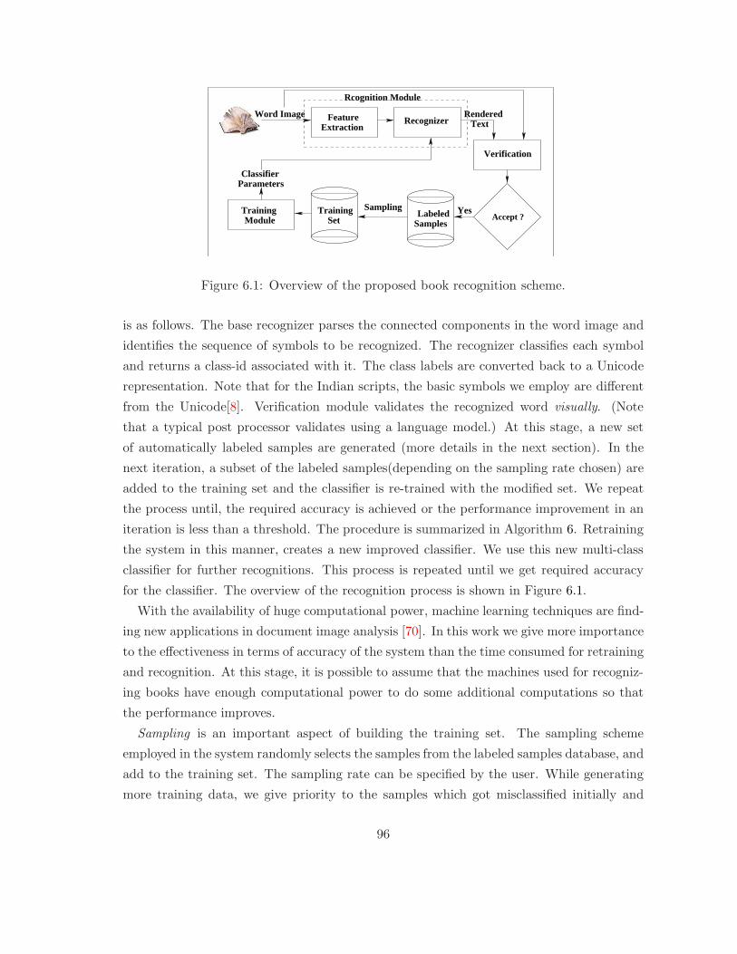
SamplesLabeledTraining

Set

Verification

Accept ?Training Module

ClassifierParameters

Feature Extraction

Recognizer

Sampling Yes

Word Image Rendered

Rcognition Module

Text

Figure 6.1: Overview of the proposed book recognition scheme.

is as follows. The base recognizer parses the connected components in the word image and

identifies the sequence of symbols to be recognized. The recognizer classifies each symbol

and returns a class-id associated with it. The class labels are converted back to a Unicode

representation. Note that for the Indian scripts, the basic symbols we employ are different

from the Unicode[8]. Verification module validates the recognized word visually. (Note

that a typical post processor validates using a language model.) At this stage, a new set

of automatically labeled samples are generated (more details in the next section). In the

next iteration, a subset of the labeled samples(depending on the sampling rate chosen) are

added to the training set and the classifier is re-trained with the modified set. We repeat

the process until, the required accuracy is achieved or the performance improvement in an

iteration is less than a threshold. The procedure is summarized in Algorithm 6. Retraining

the system in this manner, creates a new improved classifier. We use this new multi-class

classifier for further recognitions. This process is repeated until we get required accuracy

for the classifier. The overview of the recognition process is shown in Figure 6.1.

With the availability of huge computational power, machine learning techniques are find-

ing new applications in document image analysis [70]. In this work we give more importance

to the effectiveness in terms of accuracy of the system than the time consumed for retraining

and recognition. At this stage, it is possible to assume that the machines used for recogniz-

ing books have enough computational power to do some additional computations so that

the performance improves.

Sampling is an important aspect of building the training set. The sampling scheme

employed in the system randomly selects the samples from the labeled samples database, and

add to the training set. The sampling rate can be specified by the user. While generating

more training data, we give priority to the samples which got misclassified initially and

96

Algorithm 6 Algorithm for adaptation in book recognizer.

1: Input: Word images from the books.

2: Find the connected components(symbols).

3: Recognize each symbol using the classifier and get the class-id.

4: Map the class-ids to Unicode(text) and render the text to obtain a word image.

5: Verification module takes the input word image and the rendered word image to matches

both with a dynamic programming based algorithm.

6: The matched samples from the original word image are stored in a labeled images

database.

7: The samples are randomly selected from the database (according to the sampling rate

selected) and added to training set.

8: Train the classifier with new samples and use this new classifier for further classification.

9: Repeat the steps 2-7 until the required accuracy is achieved or the performance im-

provement is less than a threshold.

correctly classified in subsequent iterations. This is done by restricting the sampling from

newly labeled samples in the labeled samples database at each iteration.

6.3 Verification Scheme

A dynamic programming (DP) based verification module acts as the post-processor for our

system. In contrast to the conventional post-processing methods based on the dictionary

look-up, our method uses an image based matching technique for verification. The input of

the verification module is a word image and the corresponding Unicodes from the recognizer.

The output Unicodes are rendered to get an image, which is matched with the input word

image. The output of the verification module is a set of labeled samples from the word

image. Note that the purpose of the verification module is to provide labeled data for

retraining the classifier in the next iteration and thus improving the performance of the

recognition module. We need to make sure that correct samples are selected in the training

set.

In the DP table, each cell is filled with the matching cost of connected components in

the rendered and original word image. In our DP table, diagonal elements represent the

one-to-one matching of the symbols from the original image and corresponding rendered

image. Consider a simple case, where the input word image does not have any cut or merge.

In this case a high score in the diagonal element refers to a mismatch and a low score refers

97

to the match, as shown in Figure 6.2. A match in a diagonal cell refers to the correct

classification in the recognition and the mismatch refers to the misclassification.

U+0D0E ; U+0D28 ; U+0D4D ; U+0D28 ;U+0D3E ; U+0D32 ; U+0D28 ; U+200D ;

FeatureExtraction

RenderedWord Image Feature

Extraction

fik1, f ik2 ... f iknikF =

Fj2

Fj1

Fj3

Fj4

Fi1 Fi2 Fi3 Fi4

Component AnalysisConnected

Component AnalysisConnected

1

2 1

1

2

110 1

2 0

10

1

3 0

Render the Unicodeinto an image

Input Word Image

DP based Matching,

OCR output of the word (Unicode)

Figure 6.2: An Example of a dynamic programming based verification procedure. Word

image is matched with an image rendered out of the recognized text.

Though the focus of this work is not to recognize the degraded characters with cuts and

breaks, our verification algorithm identifies such samples, and avoid them in the sampling

process. A cut or merge results in the non-diagonal path in the dynamic programming. In

the case of cuts, two or more image components may correspond to one rendered component.

The DP that we employed is different from the popular DP algorithm (used for string

matching) in the following aspects: (a) We obtain cuts and merges instead of deletions and

insertions in a normal DP algorithm. (b) The matching is done in the image domain to find

the match scores in DP. (c) The computation of matching cost is different for non-diagonal

elements. Algorithm 7 gives the details of the DP based word matching process.

The verification module uses simple and structural features. This module performs well,

even if the characters are similar. In our implementation, we assume that a character can

get cut only into two pieces and the merges can happen only between two characters.

98

Algorithm 7 Algorithm for Verification as post-processor.

1: Input: Word image and the corresponding text from the Recognizer.2: Render the text to get a word image.3: Find the connected components of both original and rendered word images.4: Create the Dynamic Programming based Cost table, by matching the symbols.5: Fill the cost values in the table C(i, j) as,

C(i, j) = min

C(i− 1, j − 1) + MC(Si, Kj)C(i− 1, j) + MC((Si−1, Si), Kj)C(i, j − 1) + MC(Si, (Kj−1, Kj))

where, MC(Si, Kj) is the matching Cost of symbol Si in the text(rendered as image) withsymbol Kj in the original image.Matching Cost will be 0 if the two symbols matches, otherwise matching cost will be 1.

6: Get the matching String by reconstructing the path, by following the minimum cost path.7: Output the text that caused the minimum path as recognized text.

6.4 Results and Discussions

We have conducted our experiments on five Malayalam books. For the automatic evaluation

of performance, all these books are annotated apriori. The annotation is done as a part of

a larger activity [33]. The quality of the images in the corpus vary widely. These books

contain more than 500, 000 symbols to recognize.

Book title # Pages # Words # Symbols

Book 1 96 11,404 74, 774

Book 2 119 20,298 147,652

Book 3 84 10,585 83,914

Book 4 175 21,292 152,204

Book 5 94 12,111 92,538

Table 6.1: Details of the books used for the experiments.

In this work, our focus is on improving the classification accuracy of these symbols rather

than recognizing degraded images. Malayalam has 56 basic alphabets in its character set, in

addition to a large number of conjunct characters. We have considered a total of 205 classes

for our experiments, which includes, all the basic alphabets, popular conjunct characters,

punctuations, numerals etc. Table 6.1 summarizes the details of the books used for the

experiments.

Input to our system is a set of binary document images. After word-level segmentation,

the connected components are identified in each of the word images. They form the basic

symbols for classification. The symbols are then scaled to 20 × 20 pixels size keeping the

99

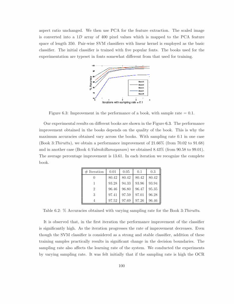
aspect ratio unchanged. We then use PCA for the feature extraction. The scaled image

is converted into a 1D array of 400 pixel values which is mapped to the PCA feature

space of length 350. Pair-wise SVM classifiers with linear kernel is employed as the basic

classifier. The initial classifier is trained with five popular fonts. The books used for the

experimentation are typeset in fonts somewhat different from that used for training.

Figure 6.3: Improvement in the performance of a book, with sample rate = 0.1.

Our experimental results on different books are shown in the Figure 6.3. The performance

improvement obtained in the books depends on the quality of the book. This is why the

maximum accuracies obtained vary across the books. With sampling rate 0.1 in one case

(Book 3:Thiruttu), we obtain a performance improvement of 21.66% (from 70.02 to 91.68)

and in another case (Book 4:ValmikiRamayanam) we obtained 8.43% (from 90.58 to 99.01).

The average percentage improvement is 13.61. In each iteration we recognize the complete

book.

# Iteration 0.01 0.05 0.1 0.3

0 80.42 80.42 80.42 80.42

1 93.28 94.33 93.96 93.94

2 96.46 96.80 96.47 95.35

3 97.41 97.59 97.01 96.28

4 97.52 97.69 97.26 96.46

Table 6.2: % Accuracies obtained with varying sampling rate for the Book 3:Thiruttu.

It is observed that, in the first iteration the performance improvement of the classifier

is significantly high. As the iteration progresses the rate of improvement decreases. Even

though the SVM classifier is considered as a strong and stable classifier, addition of these

training samples practically results in significant change in the decision boundaries. The

sampling rate also affects the learning rate of the system. We conducted the experiments

by varying sampling rate. It was felt initially that if the sampling rate is high the OCR

100

will learn fast. However, in our experiments the change in learning rate with the change

in the sampling rate was marginal (Refer Table 6.2). This is because additional samples of

the same font/style do not improve the classifier significantly. This also means that, we can

select a low sampling rate and reduce the training time.

Figure 6.4(a) shows a character that is correctly classified after improvement. In Fig-

ure 6.4(b) the character is distorted and so that even after improvement the classifier is not

able to recognize this case. In Figure 6.4(c) there is cut in the character so that each com-

ponent is classified as different classes. Similarly Figure 6.4(d) shows a failure case occurred

because of merge. One of the holes in the character shown in Figure 6.4(e) is filled, so that

it is recognized as another character.

Samples Classified as Correct Class

(a)

(c)

(e)

(d)

(b)

Figure 6.4: Examples of characters tested.

It is observed that, in the first iteration the performance improvement of the classifier is

very high, reaching to high 90’s, and as the number of iterations increases, the improvement

decreases, where the recognition process terminates. The model obtained at this stage is the

best updated knowledge we can come up for the given book (or document image collection).

6.5 Summary

In this Chapter, we propose a novel system for adapting a classifier for recognizing symbols

in a book. We employed a verification module as a post-processor for the classifier, and

make use of an automatic learning framework for the continuous improvement of classifica-

tion accuracy. We obtain an average improvement of 14% in classification accuracy. This

demonstrates that the proposed approach is promising for the recognition of books.

101

Chapter 7

Conclusions

7.1 Summary and Conclusions

This thesis proposes a classifier system for effectively and efficiently solving the character

recognition problem, when the character set is very large(in the order of hundreds). The

major contributions of this thesis are: (1). Large dataset generation. (2). Approaches

to solve large class problems. (3). Performance evaluation on a huge dataset (Malayalam

books).

We generated a large dataset for training and testing the OCR system, using a DP based

approach. we conducted empirical study on character classification problem focusing on

Indian scripts. The dimensions of the study included performance of classifiers using differ-

ent features, scalability of classifiers, sensitivity of features on degradation, generalization

across fonts and applicability across five scripts etc. We have demonstrated that with a rich

feature space, the problem is solvable with an acceptable performance using state of the art

classifiers like SVMs.

This data structure is applicable to any multiclass classification technique that builds

the solution on binary SVMs. We had shown that our data structure reduces both space

and time complexity significantly on multiclass problems. We explain an OCR architecture

based on SVM pair wise classifiers with DDAG architecture.

We carried out our classification experiments on a character recognition data set, with

more than 200 classes and 10 million examples. We tested our system on real document

images scanned from twelve Malayalam books, which comes out to be more than 2000

pages. We achieved an average error rate of 4.75 on these books. We conduct extensive

experiments to study the implications of various parameters in design of computationally

102

efficient and yet effective classifier. We also extend our classifier to continuously improve

the performance by providing feedback and retraining the classifier.

7.2 Future Scope

This work opens up many interesting problems in document understanding in the Indian

language context.

• Extend the features and classifier to support more fonts and old lipi characters.

• More script specific techniques at pre-processing stage.

• A strong post-processor based on language models. Also, a strong word recognizer as

a part of post-processor will improve the system.

• Degradation handing: To handle the spurious noise, cuts and merges in the characters.

103

Bibliography

[1] A. K. Jain, R. P. W. Duin, and J. Mao, “Statistical pattern recognition: A review,”

in IEEE Transactions on Pattern Analysis and Machine Intelligence, vol. 22(1), 2000,

pp. 4–37. 1

[2] R. O. Duda, P. E. Hart, and D. G. Stork, Pattern Classification. Wiley-Interscience

Publication, 2000. 1, 42, 43, 44, 46, 51, 64

[3] G. Nagy, “At the frontiers of ocr,” Proceedings of IEEE, vol. 80, pp. 1093–1100, July

1992. 5

[4] C. Y. Suen, S. Mori, S. H. Kim, and C. H. Leung, “Analysis and recognition of asian

scripts - the state of the art,” in ICDAR ’03: Proceedings of the Seventh Interna-

tional Conference on Document Analysis and Recognition, Washington, DC, USA,

IEEE Computer Society, 2003, p. 866. 5

[5] H. Fujisawa, “Forty years of research in character and document recognition: An in-

dustrial perspective,” PR, vol. 41, pp. 2435–2446, August 2008. 5

[6] V. Govindaraju and S. Setlur, Guide to OCR for Indic Scripts: Document Recognition

and Retrieval. Springer Publishing Company, Incorporated, 2009. 5, 42

[7] B. B. Chaudhuri, “On OCR of a printed indian script,” in Digital Document Processing:

Major Directions and Recent Advances, B. B. Chaudhuri (ed.), Springer-Verlag London

Ltd, 2007, pp. 99–119. 5, 8

[8] U. Pal and B. B. Chaudhuri, “Indian script character recognition: a survey,” Pattern

Recognition, vol. 37, no. 9, 2004. 5, 42, 55, 96

[9] V. Bansal and R. Sinha, “A devanagari ocr and a brief overview of ocr research for

indian scripts,” in Proceedings of STRANS01, held at IIT Kanpur, 2001. 5

104

[10] V. Bansal and R. M. K. Sinha, “A complete OCR for printed Hindi text in Devana-

gari script,” in Proc. of the 6th International Conference on Document Analysis and

Recognition (ICDAR), 2001, pp. 800–804. 5, 6

[11] B. B. Chaudhuri and U. Pal, “An OCR system to read two Indian language scripts:

Bangla and Devanagari (Hindi),” in Proc. of the 4th International Conference on Doc-

ument Analysis and Recognition (ICDAR), 1997, pp. 1011–1015. 5, 8

[12] B. B. Chaudhuri and U. Pal, “A complete printed Bangla OCR system,” Pattern

Recognition, vol. 31, no. 5, pp. 531–549, 1997. 5, 6

[13] U. Pal and A. Sarkar, “Recognition of printed Urdu script,” in Proc. of the 7th Inter-

national Conference on Document Analysis and Recognition (ICDAR), 2003, pp. 1183–

1187. 5, 6

[14] V. Bansal and R. M. K. Sinha, “A Devanagari OCR and a brief overview of OCR

research for Indian scripts,” in Proc. of the Symposium on Translation Support Systems,

2000. 6

[15] U. Pal and B. Chaudhuri, “Printed Devanagiri Script OCR System,” Vivek, vol. 10,

no. 2, pp. 12–24, 1997. 6

[16] G. S. Lehal and C. Singh, “A complete OCR system for Gurmukhi script,” in Structural,

Syntactic and Statistical Pattern Recognition, T. Caelli, A. Amin, R.P.W. Duin, M.

Kamel and D. de Ridder (Eds.), Lecture Notes in Computer Science, 2002, pp. 344–352.

6, 7

[17] G. S. Lehal and C. Singh, “A Gurmukhi script recognition system,” in Proc. of the

15th International Conference on Pattern Recognition (ICPR), 2000, pp. 557–560. 6

[18] S. Antanani and L. Agnihotri, “Gujarati character recognition,” Proc. of the 5th In-

ternational Conference on Document Analysis and Recognition (ICDAR), pp. 418–421,

1999. 6, 7

[19] S. Mohanty and H. K. Behera, “A complete OCR development system for Oriya script,”

in Proc. of symposium on Indian Morphology, phonology and Language Engineering,

2004. 6, 7

[20] B. B. Chaudhuri, U. Pal, and M. Mitra, “Automatic recognition of printed Oriya

script,” in Proc. of the 6th International Conference on Document Analysis and Recog-

nition (ICDAR), 2001, pp. 795–799. 6

105

[21] K. H. Aparna and V. S. Chakravarthy, “A complete OCR system development of Tamil

magazine documents,” in Tamil Internet, Chennai, Tamilnadu, India, 2003. 6, 7

[22] C. V. Lakshmi and C. Patvardhan, “A complete multi-font OCR systems for printed

Telugu text,” in Language Engineering Conference, 2002. 6

[23] A. Negi, C. Bhagvathi, and B. Krishna, “An OCR system for Telugu,” in Proc. of the

6th International Conference on Document Analysis and Recognition (ICDAR), 2001,

pp. 1110–1114. 6, 7, 48

[24] P. Rao and T. Ajitha, “Telugu script recognition - A feature based approach,” in Inter-

national Conference on Document Analysis and Recognition (ICDAR), 1995, pp. 323–

326. 6

[25] V. N. Manjunath, P. S. Aradhyal, G. H. Kumar, and S. Noushathl, “Fisher linear dis-

criminant analysis based technique useful for efficient character recognition,” in Proc.

of the 4th International Conference on Intelligent Sensing and Information Processing,

2006, pp. 49–52. 6

[26] T. Ashwin and P. Sastry, “A font and size-independent ocr system for kannanda doc-

uments using svm,” in Sadhana, vol. 27, 2002. 6

[27] K. Jithesh, K. G. Sulochana, and R. R. Kumar, “Optical character recognition (OCR)

system for Malayalam language,” in National Workshop on Application of Language

Technology in Indian Languages, 2003. 6, 7

[28] G. Prathap, “Indian language document analysis and understanding,” Special Issue of

Sadhana, vol. 27, 2002. 7

[29] T. V. Ashwin and P. S. Sastry, “A font and size independent OCR system for printed

Kannada documents using support vector machines,” Special Issue of Sadhana, vol. 27,

pp. 35–58, 2002. 7

[30] C. V. Jawahar, M. N. S. S. K. P. Kumar, and S. S. R. Kiran, “A Bilingual OCR for

Hindi-Telugu Documents and its Applications,” in Proc. of the International Confer-

ence on Document Analysis and Recognition (ICDAR), 2003, pp. 408–412. 8

[31] M. N. S. S. K. P. Kumar and C. V. Jawahar, “Design of hierarchical classifier with

hybrid architectures,” in Proc. of 1st Int. Conf. on Pattern Recognition and Machine

Intelligence (PReMI), 2005, pp. 276–279. 8

106

[32] T. K. Chalasani, A. M. Namboodiri, and C. V. Jawahar, “Support vector machine

based hierachical classifieds for large class problems,” in proceedings of International

Conference on Advances in Pattern Recognition (ICAPR), 2007. 8

[33] C. V. Jawahar and A. Kumar, “Content-level annotation of large collection of printed

document images,” in International Conference on Document Analysis and Recognition

(ICDAR), 2007, pp. 799–803. 15, 92, 99

[34] M. Meshesha and C. V. Jawahar, “Matching word images for content-based retrieval

from printed document images,” Int. J. Doc. Anal. Recognit., vol. 11, no. 1, pp. 29–38,

2008. 17, 57

[35] A. Balasubramanian, M. Meshesha, and C. V. Jawahar, “Retrieval from document

image collections,” in In: Proc. DAS, Springer, 2006, pp. 1–12. 31

[36] T. M. Rath and R. Manmatha, “Word image matching using dynamic time warping,”

Computer Vision and Pattern Recognition, IEEE Computer Society Conference on,

vol. 2, p. 521, 2003. 31

[37] T. M. Rath and R. Manmatha, “Features for word spotting in historical manuscripts,”

in ICDAR ’03: Proceedings of the Seventh International Conference on Document

Analysis and Recognition, Washington, DC, USA, IEEE Computer Society, 2003,

p. 218. 31

[38] R. King, C. Feng, and A. Shutherland, “Statlog: comparison of classification algorithms

on large real-world problems,” AAI, vol. 9, pp. 259–287, June 1995. 42

[39] R. Caruana and A. Niculescu-Mizil, “An empirical comparison of supervised learning

algorithms,” in proceedings of International Conference on Machine Learning (ICML),

2006. 42, 64

[40] Y. e. Lecun, “Learning algorithms for classification: A comparison on handwritten

digit recognition,” in Neural Networks: The Statistical Mechanics Perspective, 1995,

pp. 261–276. 42, 46

[41] A. Asuncion and D.J.Newman. “UCI machine learning repository,”,”. WWW page,

2007. 42, 71

[42] S. Arya and H.-Y. A. Fu, “Expected-case complexity of approximate nearest neighbor

searching,” in proceedings of Symposium on Discrete Algorithms, 2000, pp. 379–388.

44

107

[43] T.-S. Lim, W.-Y. Loh, and Y.-S. Shih, “An empirical comparison of decision trees and

other classification methods,” Tech. Rep. 979, Madison, WI, 30 1997. 44

[44] S. K. Murthy, S. Kasif, S. Salzberg, and R. Beigel, “Oc1: A randomized algorithm for

building oblique decision trees,” tech. rep., 1993. 44

[45] S. Haykin, Neural Networks - A Comprehensive Foundation, 2nd ed. Prentice-Hall,

Englewood Cliffs, 1998. 45

[46] L. Bottou, C. Cortes, J. Denker, H. Drucker, I. Guyon, L. Jackel, Y. LeCun, U. Muller,

E. Sackinger, P. Simard, and V. Vapnik, “Comparison of classifier methods: a case

study in handwritten digit recognition,” in Proc. of the International Conference on

Pattern Recognition (ICPR), vol. II, Jerusalem, IEEE, October 1994, pp. 77–82. 45

[47] Y. LeCun, L. D. Jackel, L. Bottou, A. Brunot, C. Cortes, J. S. Denker, H. Drucker,

I. Guyon, U. A. Muller, E. Sackinger, P. Simard, and V. Vapnik, “Comparison of

learning algorithms for handwritten digit recognition,” in proceedings of International

Conference on Artificial Neural Networks, Paris, EC2 & Cie, 1995, pp. 53–60. 45

[48] A. Caldern, S. Roa, and J. Victorino, “Handwritten digit recognition using convo-

lutional neural networks and gabor filters,” in INTERNATIONAL CONGRESS ON

COMPUTATIONAL INTELLIGENCE, 2003. 46

[49] N. Cristianini and J. Shawe-Taylor, An Introduction to Support Vector Machines and

Other Kernel-based Learning Methods. Cambridge University Press, March 2000. 47

[50] T. M. Mitchell, Machine Learning. New York: McGraw-Hill, 1997. 47

[51] J. Platt, N. Cristianini, and J. Shawe-Taylor, “Large margin dags for multiclass classi-

fication,” in proceedings of Advances in Neural Information Processing Systems, 2000,

pp. 547–553. 47, 65, 77

[52] O. Trier, A. Jain, and A. Taxt, “Feature extraction methods for character recognition

- a survey.,” in Pattern Recognition 29,, 1996, pp. 641–662. 48

[53] W. Gonzalez, Digital Image Processing. Massachusetts: Addison Wesley, 1992. 48, 49,

50

[54] A. Khotanzad and Y. H. Hong, “Invariant image recognition by zernike moments,”

IEEE Trans. Pattern Anal. Mach. Intell., vol. 12, no. 5, pp. 489–497, 1990. 49

108

[55] I. Popivanov and R. J. Miller, “Similarity search over time series data using wavelets,”

in Proc. of the 18th Int. Conf. on Data Engineering, 2002, pp. 212–221. 49, 50

[56] E. Bingham and H. Mannila, “Random projection in dimensionality reduction: applica-

tions to image and text data,” in KDD ’01: Proceedings of the seventh ACM SIGKDD

international conference on Knowledge discovery and data mining, New York, NY,

USA, ACM, 2001, pp. 245–250. 51

[57] W. Johnson and J. Lindenstrauss, “Extensions of lipshitz mapping into hilbert space.,”

In Conference in modern analysis and probability, vol. 26 of Contemporary Mathemat-

ics, pp. 189–206, 1984. 52

[58] R. Brown, “The fringe distance measure: An easily calculated image distance measure

with recognition results comparable to gaussian blurring,” SMC, vol. 24, pp. 111–115,

1994. 52

[59] Q. Zheng and T. Kanungo, “Morphological degradation models and their use in doc-

ument image restoration,” in proceedings of International Conference on Image Pro-

cessing (ICIP), 2001, pp. 193–196. 56

[60] R. Caruana and A. Niculescu-Mizil, “Data mining in metric space: An empirical anal-

ysis of supervised learning performance criteria,” in Knowledge Discovery and Data

Mining, 2004. 64

[61] V. Vapnik, “The nature of statistical learning theory,” in second ed. Springer Verlag,

1999. 64

[62] N. Cristianini and J. Shawe-Taylor, An Introduction to Support Vector Machines and

Other Kernel-based Learning Methods. 2000. 65

[63] C.-W. Hsu and C.-J. Lin, “A comparison of methods for multiclass support vector

machines,” in IEEE Transactions on Neural Networks, vol. 13, 2002, pp. 415–425. 65

[64] K.-B. Duan and S. S. Keerthi, “Which is the best multiclass svm method? an empirical

study,” in proceedings of Multiple Classifier Systems(MCS), June 2005, pp. 278–285.

65

[65] C. J. C. Burges, “Simplified support vector decision rules,” in proceedings of Interna-

tional Conference on Machine Learning (ICML), vol. 13, 1996. 65

109

[66] T. Downs, K.E.Gates, and A. Masters, “Exact simplification of support vector so-

lutions,” Journal of Machine Learning Research, vol. 2, pp. 293–297, 2001. 65, 73,

76

[67] T. Joachims, “Making large-scale svm learning practical,” in Advances in Kernel Meth-

ods - Support Vector Learning,MIT-Press, 1999. 70

[68] C.-C. Chang. “Libsvm,”,”. http://www.csie.ntu.edu.tw/∼cjlin/libsvm/, 2008.

70

[69] Y. Xu and G. Nagy, “Prototype extraction and adaptive ocr,” IEEE Trans. on Pattern

Analysis and Machine Intelligence (PAMI), vol. 21, no. 12, pp. 1280–1296, 1999. 94

[70] C. L. Liu and H. Fujisawa, “Classification and learning methods for character recogni-

tion :Advances and remaining problems,” in Neural Networks and Learning in Docu-

ment Analysis and Recognition. 2008, pp. 139–161. 94, 96

[71] K. P. Sankar, V. Ambati, L. Pratha, and C. V. Jawahar, “Digitizing a million books:

Challenges for document analysis,” in International Workshop on Document Analysis

Systems (DAS), 2006, pp. 425–436. 94

[72] M. Meshesha and C. V. Jawahar, “Self adaptable recognizer for document image collec-

tions,” in proceedings of Pattern Recognition and Machine Intelligence, 2007, pp. 560–

567. 94, 95

[73] P. Xiu and H. S. Baird, “Whole-book recognition using mutual-entropy-driven model

adaptation,” in Document Recognition and Retrieval XV. Proc. of SPIE, 2008. 94, 95

[74] V. Rasagna, A. Kumar, C. V. Jawahar, and R. Manmatha, “Robust recognition of

documents by fusing results of word clusters,” in ICDAR ’09: Proceedings of the 2009

10th International Conference on Document Analysis and Recognition, Washington,

DC, USA, IEEE Computer Society, 2009, pp. 566–570. 95

110

111

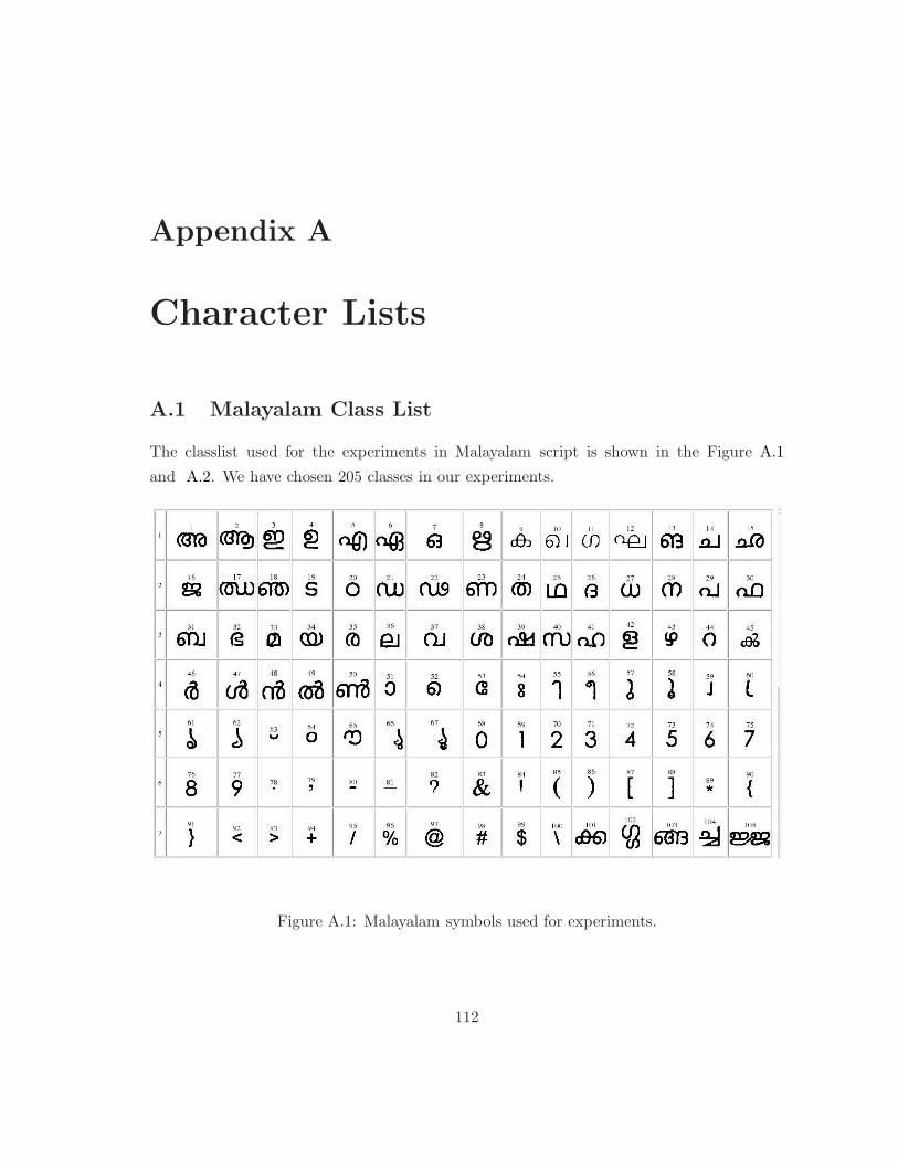
Appendix A

Character Lists

A.1 Malayalam Class List

The classlist used for the experiments in Malayalam script is shown in the Figure A.1

and A.2. We have chosen 205 classes in our experiments.

Figure A.1: Malayalam symbols used for experiments.

112

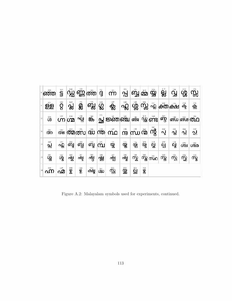
Figure A.2: Malayalam symbols used for experiments, continued.

113

Appendix B

Publications Related to This Work

The work done during my masters has been disseminated to the following conferences:

1. Neeba N.V, C.V Jawahar, Empirical Evaluation of Character Classification

Schemes, The seventh International Conference on Advances in Pattern Recognition

(ICAPR ’09), Feb . 4-6, 2009, Kolkotta, India. [PDF].

2. Neeba N.V, C.V Jawahar, Recognition of Books by Verification and Retrain-

ing, The nineteenth International Conference on Pattern Recognition (ICPR ’08),

Dec. 8-11,2008, Florida, USA. [PDF].

3. P.Ilayaraja, Neeba N.V, C.V Jawahar, Efficient Implementation of SVM for

Large Class Problems, The nineteenth International Conference on Pattern Recog-

nition(ICPR ’08), Dec. 8-11,2008, Florida, USA. [PDF].

We have also written a book chapter:

• Neeba N.V, A.M Namboodiri, C.V Jawahar and P.J Narayanan, Recognition of

Malayalam documents, Guide to OCR for Indic Scripts, Pages 125-146, 2009.

114