Large-Scale Image Classification using High Performance Clustering

Bingjing Zhang, Judy Qiu, Stefan Lee, David Crandall Department of Computer Science and Informatics

Indiana University, Bloomington {zhangbj, xqiu, steflee, djcran}@indiana.edu

Abstract— Computer vision is being revolutionized by the incredible volume of visual data available on the Internet. A key part of computer vision, data mining, or any Big Data problem is the analytics that transforms this raw data into understanding, and many of these data mining approaches require iterative computations at an unprecedented scale. Often an individual iteration can be specified as a MapReduce computation, leading to the iterative MapReduce program-ming model for efficient execution of data-intensive iterative computations. We propose the Map-Collective model as a generalization of our earlier Twister system that is interoperable between HPC and cloud environments. In this paper, we study the problem of large-scale clustering, applying it to cluster large collections of 10-100 million social images, each represented as a point in a high dimensional (up to 2048) vector space, into 1-10 million clusters. This K-means application needs 5 stages in each iteration: Broadcast, Map, Shuffle, Reduce and Combine, and this paper presents new collective communication approaches optimized for large data transfers. Furthermore one needs additional communication patterns from those familiar in MapReduce, and we develop collectives that integrate capabilities developed by the MPI and MapReduce communities. We demonstrate that a topology-aware and pipeline-based broadcasting method gives better performance than both MPI and other (Iterative) MapReduce systems. We present early results of an end-to-end computer vision application and evaluate the quality of the resulting image classifications, showing that increasing the number of feature clusters leads to improved classifier accuracy.

Keywords-Social Images; Data Intensive; High Dimension; Iterative MapReduce; Collective Communication

I. INTRODUCTION The rate of data generation now exceeds the growth of

computational power predicted by Moore’s law. Mining and analyzing these massive data sources to translate large-scale data into knowledge-based innovation represents a major computational challenge. MapReduce frameworks have become popular in recent years for their scalability and fault tolerance in large data processing and for their simplicity in the programming interface. Hadoop [1], an open source implementation following Google’s original MapReduce concept [2], has been widely used in industry and academia.

But MapReduce does not directly address iterative solvers and basic matrix primitives, which Intel’s RMS (Recognition, Mining and Synthesis) taxonomy [3] identifies as common computing kernels for computer vision, rendering, physical simulation, financial analysis and data mining. These and other observations [7] suggest that iterative data processing will be important to a spectrum of e-Science and e-Research applications as a kernel framework for large-scale data processing. Several frameworks designed

for iterative MapReduce have been proposed to solve this problem, including Twister [4], Spark [5], HaLoop [6], etc. For example, the initial version of Twister optimized data flow and reduced data transfer between iterations by caching invariant data in the local memory of compute nodes. However, it did not support the communication patterns needed in many applications. We observe that a systematic approach to collective communication is essential in many iterative algorithms. Thus we generalize the (iterative) MapReduce concept to Map-Collective, since large collectives are distinctive features of data intensive applications [8][9].

Large-scale computer vision is one application that involves big data and often needs iterative solvers, such as large-scale clustering stages. This application produces challenges requiring both new algorithms and optimizing parallel execution involving very large collective communication steps. We have addressed overall performance with an extension of Elkan's algorithm [10] to drastically speed up the computing (Map) step of clustering by use of the triangle inequality to remove unnecessary computation [8]. But this improvement increased the need for efficient communication, which is a major focus of this paper. Note that communication has been well studied, especially in MPI, but large-scale computer vision stresses different usage modes and message sizes from most previous applications.

In this paper, we study the characteristics of a large-scale image clustering application and identify performance issues of collective communication. Our work is presented in the context of Twister, but the analysis is applicable to MapReduce and other data-centric computation solutions. In particular, the vision application requires 7 million image feature vectors to be clustered. We execute the application on 1000 cores (125 8-core nodes) with 10,000 Map tasks. The root node must broadcast 512 MB of data to all compute nodes, making sequential broadcast costly. In aggregation, 20 TB of intermediate data needs to be transferred from Map stage. Here we propose a topology-aware pipeline method to accelerate broadcast by a factor of over 120 compared with the sequential algorithm, and comparable with classic MPI methods [11] by slight (20%) outperformance in C and large factors over Java MPJ. We also use 3-stage aggregation to efficiently reduce intermediate data size by at least 90% within each stage. These methods provide important collective communication capabilities to our new iterative Map-Collective framework for data intensive applications. We evaluate our new methods on the PolarGrid cluster.

II. MOTIVATING APPLICATION: LARGE-SCALE VISION Computer vision is being revolutionized by the volume

of visual data on the Internet, including 500 million images uploaded every day to Facebook, Instagram and Snapchat, and 100 hours of video uploaded to YouTube every minute. These huge collections of social imagery are motivating many large scale computer vision studies that can benefit from the infrastructure studied here. A major goal of these projects is to help organize photo collections, for instance by automatically determining the type of scene [12], recognizing common objects [13] and landmarks [14], determining where on earth a photo was taken [16] [17], and so on.

A. Scene Type Recognition Here we consider the specific problem of recognizing

two general properties of a photo: whether it was taken in an urban or rural environment, and whether it was taken in a mountainous or relatively “flat” locale. A popular approach for visual classification tasks involves embedding images in a more discriminative space by representing them as collections of discriminative, invariant local image features. This is known as the Bag of Words (BoW) model, and is borrowed from techniques in information retrieval that represent documents as an unordered collection of words. To make this analogy work, we need to identify basic distinguishing features or visual words so that images can be encoded as histograms over this vocabulary [17].

One way of producing this vocabulary is to sample small patches from many images, perform clustering, and then use each of the cluster centroids to define a visual word. In our application, we sample five patches from each of 12 million images and describe each patch using the Histograms of Oriented Gradients (HOG) features [18]. HOG characterizes the local image features as a distribution of local edge gradients (see Figure 1), and produces a 512-dimensional vector for each patch. Once the vocabulary is generated, any image can be represented as a histogram over this vocabulary: given an image, we densely sample patches, compute HOG vectors from these patches, assign each vector

to its nearest centroid in the vocabulary, and then count the number of times each centroid occurs. Support Vector Machines (SVM) [19] are trained on these features to learn a discriminative classifier between the image classes of interest (e.g. rural vs. urban).

B. Large-scale Image Feature Clustering A major challenge with this approach is the clustering

step, as ideally we would like to cluster billions of patches into millions of centroids. We confront this computational challenge by performing K-means clustering as a chain of Map computations separated by collective communications (Figure 2). The input data consists of a large number of feature vectors each with 512 dimensions. We compute Euclidean distances between feature vectors and cluster centers (centroids). Since the vectors are static over iterations, we partition (decompose) the vectors and cache each partition in memory, and assign a Map task to it during job configuration. At each iteration, the iteration driver broadcasts centroids to all Map tasks. Each Map task then assigns feature vectors to the nearest cluster. Map tasks calculate the sum of vectors associated with each cluster and count the total number of such vectors. To simplify the discussion, we only describe 1-stage aggregation here instead of 3-stage aggregation which is used in real implementation. The aggregation stage processes the output collected from each Map task and calculates new cluster centers by adding all partial sums of cluster center values together, then dividing by the total number of points in the cluster. By combining these new centroids from Reduce tasks, the iteration driver gets updated centroids and control flow enters the next iteration (Table I).

Another major challenge of this application is the amount of feature data. Currently we have nearly 1 TB, corresponding to 60 million HOG feature vectors, and we expect problems to grow in size by one to two orders of magnitude. For such a large amount of input data, we can increase the number of machines to reduce the data size per node, but the total data size (of cluster centers) transferred in broadcasting and aggregation still grows as the number of centers multiplies.

Figure 1. Workflow of the vocabulary learning application.

Figure 2. Image clustering control flow in Twister with the new local aggregation feature in Map stage.

For example, suppose we were to cluster 7 million 512- dimensional vectors into 1 million clusters. In one iteration, the execution is done on 1,000 cores in 10 rounds with a total of 10,000 Map tasks. Each task only needs to cache 700 vectors (358KB) and each node needs to cache 56K vectors, about 30MB in total. But in broadcast, the size of 1 million cluster centers is about 512MB. Therefore the centroids data per task received through broadcasting is much larger than the image feature vectors per task. Since each Map task needs a full copy of the centroids, the total data sent through broadcasting grows with the problem size and the number of nodes. For the example above, the total broadcast is about 64 GB (because Map tasks are executed as threads, broadcast data can be shared among tasks on one node).

We now reach the aggregation stage. Here each Map task generates about 2 GB of intermediate data, for a total of about 20 TB. This far exceeds the total memory size of 125 nodes (each of which has 16 GB memory; 2 TB in total), and also makes the computation difficult to scale, since the data size grows with the number of nodes. In this paper, we do 3-stage aggregation to solve this problem. In the first stage, we reduce 20 TB of intermediate data to 250 GB with local aggregation (Figure 2). But due to limited memory, 250 GB still cannot be aggregated directly on one node. Thus we further divide the output data from each Map task into 125 partitions (numbered with Partition ID 0 to 124) and use 125

tasks (1 task per node) to do group-by aggregation at the second stage. In this way, each node only processes 2 GB of data: Node 0 processes Partition 0 from all Map tasks, Node 1 processes Partition 1 from all Map tasks, and so on. The output of group-by aggregation on each node is about 4 MB, so the 125 nodes only need to gather about 512 MB to the driver in the third stage of aggregation.

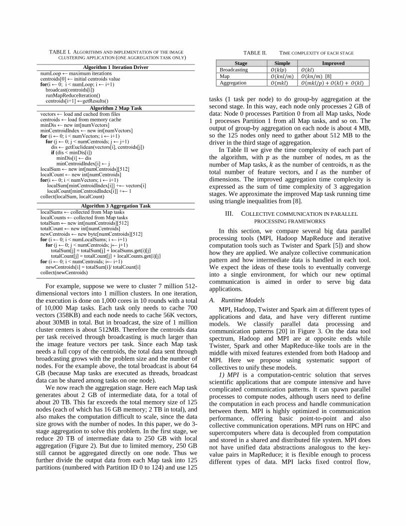
In Table II we give the time complexity of each part of the algorithm, with 𝑝𝑝 as the number of nodes, 𝑚𝑚 as the number of Map tasks, 𝑘𝑘 as the number of centroids, 𝑛𝑛 as the total number of feature vectors, and 𝑙𝑙 as the number of dimensions. The improved aggregation time complexity is expressed as the sum of time complexity of 3 aggregation stages. We approximate the improved Map task running time using triangle inequalities from [8].

III. COLLECTIVE COMMUNICATION IN PARALLEL PROCESSING FRAMEWORKS

In this section, we compare several big data parallel processing tools (MPI, Hadoop MapReduce and iterative computation tools such as Twister and Spark [5]) and show how they are applied. We analyze collective communication pattern and how intermediate data is handled in each tool. We expect the ideas of these tools to eventually converge into a single environment, for which our new optimal communication is aimed in order to serve big data applications.

A. Runtime Models MPI, Hadoop, Twister and Spark aim at different types of

applications and data, and have very different runtime models. We classify parallel data processing and communication patterns [20] in Figure 3. On the data tool spectrum, Hadoop and MPI are at opposite ends while Twister, Spark and other MapReduce-like tools are in the middle with mixed features extended from both Hadoop and MPI. Here we propose using systematic support of collectives to unify these models.

1) MPI is a computation-centric solution that serves scientific applications that are compute intensive and have complicated communication patterns. It can spawn parallel processes to compute nodes, although users need to define the computation in each process and handle communication between them. MPI is highly optimized in communication performance, offering basic point-to-point and also collective communication operations. MPI runs on HPC and supercomputers where data is decoupled from computation and stored in a shared and distributed file system. MPI does not have unified data abstractions analogous to the key-value pairs in MapReduce; it is flexible enough to process different types of data. MPI lacks fixed control flow,

TABLE II. TIME COMPLEXITY OF EACH STAGE

Stage Simple Improved Broadcasting 𝑂𝑂(𝑘𝑘𝑙𝑙𝑝𝑝) 𝑂𝑂(𝑘𝑘𝑙𝑙) Map 𝑂𝑂(𝑘𝑘𝑛𝑛𝑙𝑙/𝑚𝑚) 𝑂𝑂(𝑘𝑘𝑛𝑛/𝑚𝑚) [8] Aggregation 𝑂𝑂(𝑚𝑚𝑘𝑘𝑙𝑙) 𝑂𝑂(𝑚𝑚𝑘𝑘𝑙𝑙/𝑝𝑝) + 𝑂𝑂(𝑘𝑘𝑙𝑙) + 𝑂𝑂(𝑘𝑘𝑙𝑙)

TABLE I. ALGORITHMS AND IMPLEMENTATION OF THE IMAGE CLUSTERING APPLICATION (ONE AGGREGATION TASK ONLY)

Algorithm 1 Iteration Driver numLoop ← maximum iterations centroids[0] ← initial centroids value for(i ← 0; i < numLoop; i ← i+1) broadcast(centroids[i]) runMapReduceIteration() centroids[i+1] ←getResults()

Algorithm 2 Map Task vectors ← load and cached from files centroids ← load from memory cache minDis ← new int[numVectors] minCentroidIndex ← new int[numVectors] for (i ← 0; i < numVectors; i ← i+1) for (j ← 0; j < numCentroids; j ← j+1) dis ← getEuclidean(vectors[i], centroids[j]) if (dis < minDis[i]) minDis[i] ← dis minCentroidIndex[i] ← j localSum ← new int[numCentroids][512] localCount ← new int[numCentroids] for(i ← 0; i < numVectors; i ← i+1) localSum[minCentroidIndex[i]] +← vectors[i] localCount[minCentroidIndex[i]] +← 1 collect(localSum, localCount)

Algorithm 3 Aggregation Task localSums ← collected from Map tasks localCounts ← collected from Map tasks totalSum ← new int[numCentroids][512] totalCount ← new int[numCentroids] newCentroids ← new byte[numCentroids][512] for (i ← 0; i < numLocalSums; i ← i+1) for (j ← 0; j < numCentroids; j← j+1) totalSum[j] = totalSum[j] + localSums.get(i)[j] totalCount[j] = totalCount[j] + localCounts.get(i)[j] for (i ← 0; i < numCentroids; i← i+1) newCentroids[i] = totalSum[i]/ totalCount[i] collect(newCentroids)

endowing it with the flexibility to emulate MapReduce or other user-defined models [21-23].

2) MapReduce and Hadoop: On the other hand, Hadoop is data-centric. HDFS [25] is used to store and manage big data so that users are freed from the data accessing and loading steps required in MPI. In addition, computations are performed where the data is located to promote scalability. Key-Value pairs are the core data abstraction in MapReduce. With keys, intermediate data values are labeled and regrouped automatically without explicit communication commands. Hadoop is very suitable for processing records and logs, which are easy to split into small Key-Value pairs with words or lines. A typical record or log processing task includes information extraction and regrouping, which are easily expressed in Map-Reduce: intermediate Key-Value pairs are first extracted from records and logs in Map tasks, then regrouped in shuffling, and finally processed by Reduce tasks. But Hadoop is inefficient for many applications served by MPI because its control flow is constrained to Map-Shuffle-Reduce patterns.

Differences in the algorithms and data characteristics of an application also influence scheduling. In many scientific applications, the workload can be evenly distributed across compute nodes and in-memory communication between processes happens frequently; as a result, MPI uses static scheduling. But for log and record processing, the workload in each task is hard to estimate, since some tasks generate more Key-Value pairs than others and all data exchange is based on HDFS (not in-memory communication). Because of these, Hadoop uses dynamic scheduling. Hadoop also provides task-level fault tolerance, while MPI does not.

3) Twister and Spark: Twister and Spark are somewhere between MPI and Hadoop. Twister provides an easy-to-use, data-centric solution to process big data in data mining and scientific applications. Twister’s control flow is defined by iterations of MapReduce jobs, with the output of each iteration sent to the input to the next iteration. The data in Twister is abstracted as Key-Value pairs for intermediate data regrouping as per the needs of the application, and uses static scheduling: data is pre-split and evenly distributed to nodes based on the available computing slots (the number of cores). Tasks are then sent to where the data is located.

Spark also targets iterative algorithms but also boasts flexible iteration control with separated RDD operations called transformations and actions. A RDD is an in-memory data abstraction in distributed computing with fault tolerance support. Typical operations on RDDs include MapReduce-like operations such as Map, GroupByKey (like Shuffle but without sort) and ReduceByKey (same as Reduce), and also relational database-like operations like Union, Join, and Cartesian-Product. Spark scheduling is similar to Dryad but considers available memory of RDD partitions. RDD’s lineage graph is examined to build a DAG of stages for late execution.

The Key-Value abstraction in MapReduce also requires more work in the form of partitioning before data loading, because the data abstracted in computation is usually not organized in the same way as in the file system. For

example, the data in our image clustering application is stored in a set of text files, with each file containing feature vectors generated from a set of images. The file lengths and the total number of files vary. However, in the computation we set the number of data partitions to be a multiple of the number of cores so that we can evenly distribute computation.

Ultimately we need to convert “raw” data on disks to “cooked” data ready for computation. Currently we split original data files into evenly-sized data partitions. But Hadoop can automatically load data from blocks with custom InputSplit or InputFormat classes, while MPI requires the user to split data or use special formats like HDF5 and NetCDF.

B. Collective Communication and Intermediate Data Handling

MPI researchers have made major progress on communication optimization. However MPI focuses on low latency communication, while our application is notable for large messages where latency is less relevant. With the support of high-performance hardware, communication is well optimized. Users can communicate in two ways; one is to call send/receive APIs to customize communication between processes, and another is to invoke libraries to do collective communication, which is a type of communication in which all the workers are required to participate.

Often data-centric problems run on clouds which consist of commodity machines, and the cost of transferring big intermediate data is high. For example, in our image clustering application, broadcasting about 500MB is required, and our findings show that this operation can be a great burden to current data-centric technology. This makes it necessary to systematically develop a Map-Collective approach with a wide range of collectives, and to optimize for big data instead of the MPI simulation optimizations.

There are traditionally 7 collective communication operations discussed in MPI [26]: four data redistribution operations (broadcast, scatter, gather, allgather) and three data consolidation operations (reduce(-to-one), reduce-scatter, all-reduce). Neither Hadoop, Twister, nor Spark explicitly defines all these operations. Hadoop has implicit

(a) Map Only(Pleasingly Parallel)

(b) ClassicMapReduce

(c) IterativeMapReduce

(d) Loosely Synchronous

- CAP3 Gene Analysis- Smith-Waterman

Distances- Document conversion

(PDF -> HTML)- Brute force searches in

cryptography- Parametric sweeps- PolarGrid Matlab data

analysis

- High Energy Physics (HEP) Histograms

- Distributed search- Distributed sorting- Information retrieval- Calculation of Pairwise

Distances for sequences (BLAST)

- Expectation maximization algorithms

- Linear Algebra- Data mining include K-

means clustering - Deterministic

Annealing Clustering- Multidimensional

Scaling (MDS) - PageRank

Many MPI scientific applications utilizingwide variety of communication constructs including local interactions- Solving Differential

Equations and - particle dynamics with

short range forces

Pij

Collective Communication MPI

Input

Output

map

Inputmap

reduce

Inputmap

iterations

No Communication

reduce

Figure 3. Classification of Applications

“broadcast” based on distributed cache and since Hadoop data is managed by HDFS, direct memory-to-memory collective communication does not exist. Twister and Spark supports broadcast explicitly but not allgather and allreduce. Another iterative MapReduce system, Twister4Azure [27], supports all-gather and all-reduce. In a later paper we will describe integrating these different collectives into a single system that runs on HPC clusters (Twister) and PaaS cloud systems (Twister4Azure), changing the implementation to optimize for each infrastructure. The same high level collective primitive is used on each platform with different under-the-hood optimizations.

In broadcasting, data abstraction and methods are very different across these systems: data is abstracted as an array buffer in MPI, as an HDFS file in Hadoop, and as an object in Twister and Spark (Key-Value pairs in Twister and arbitrary objects in Spark). Several algorithms are used for broadcasting. MST (Minimum-Spanning Tree) is typically used in MPI [26]. In this method, nodes form a minimum spanning tree and data is forwarded along the links. In this way, the number of nodes which have data grows in geometric progression, such that the performance model is:

𝑇𝑇𝑀𝑀𝑀𝑀𝑀𝑀(𝑝𝑝,𝑛𝑛) = ⌈𝑙𝑙𝑙𝑙𝑙𝑙2𝑝𝑝⌉(𝛼𝛼 + 𝑛𝑛𝑛𝑛) (1)

where p is the number of nodes, n is the data size, α is the communication startup time and β is the data transfer time per unit. This method is much better than simple broadcasting by reducing the complexity term p to ⌈log2p⌉. But it is still insufficient when compared with scatter-all-gather bucket algorithm. This algorithm is used in MPI for long vector broadcasting, which follows the style of “divide, distribute and gather” [28]. In the “scatter” phase, it scatters the data to all the nodes. Then in all-gather the bucket algorithm is used, which views the nodes as a chain. At each step, every node sends data to its right neighbor [31]. By taking advantage of the fact that messages traversing a link in opposite directions do not conflict, all-gather is done in parallel without any network contention. The performance model is:

𝑇𝑇𝑏𝑏𝑏𝑏𝑏𝑏𝑏𝑏𝑏𝑏𝑏𝑏(𝑝𝑝,𝑛𝑛) = (𝑝𝑝 + 𝑝𝑝 − 1)(𝛼𝛼 + 𝑛𝑛𝑛𝑛 𝑝𝑝⁄ ) (2)

In large data broadcasting, assuming α is small, the broadcasting time is about 2nβ. This is much better than the MST method because time is constant. However, it is not easy to set a global barrier between the scatter and all-gather phases in a cloud system to enable all the nodes to do all-gather at the same time. As a result, some links will have more load than others and thus cause network contention. We implemented this algorithm and provide test results on IU PolarGrid (Table III). The execution time is roughly 2𝑛𝑛𝑛𝑛, but as the number of nodes increases, it gets slightly slower.

MPI also has InfiniBand multicast-based broadcast [29]. Many clusters support hardware-based multicast, but it is not reliable: send order is not guaranteed and size of each send is limited. So after the first stage of multicasting, broadcast is enhanced with a chain-like broadcast, which is reliable

enough to make sure every process has completed receiving data. In the second stage, the nodes are formed into a virtual ring topology. Each MPI process that gets a message via multicast serves as a new “root” within the virtual ring and exchanges data to its predecessor and successor in the ring. This is similar to the bucket algorithm we discussed above.

Though the above methods are not perfect, they all reduce broadcast time to a great extent. Still, none of them are applied in data-centric solutions, where instead a simple algorithm is commonly used. Hadoop relies on HDFS to do broadcasting: the Distributed Cache is used to cache data from HDFS to local disks of the compute nodes. The API addCacheFile and getLocalCacheFiles work together to complete the process of broadcasting. There is no special optimization, and data download speed depends on the number of replicas in HDFS [25]. This method generates significant overhead (factor of p) when handling big data, as we show in our experiments. We call this a “simple algorithm” because it sends data to all nodes one by one. Initially in Twister, a single message broker is used to do broadcasting in a similar way (Figure 4). Multiple brokers in Twister or multiple replicas in HDFS could contain a simple 2-level broadcasting tree to ease performance issues, but this does not solve the problem. In the next section we propose a chain-based broadcasting algorithm suitable for cloud systems.

Meanwhile, instead of using the simple algorithm, Spark enhances broad cast speed by using BitTorrent, a well-known technology in file sharing. Spark’s broadcast programming interface is very different from MPI and Twister. Due to the mechanism of late execution, broadcast is finished not in a single step but in two stages. When broadcast is invoked, the data is not broadcast until the parallel tasks are executed. Broadcasting happens when 10 printing tasks are invoked, so it doesn’t execute on all the nodes, only those where tasks are located. The performance

Worker Node

Local Disk

Worker Pool

Twister Daemon

Master Node

Twister Driver

Main Program

B B BB

Pub/Sub Broker Network and Collective Communication Service

Worker Node

Local Disk

Worker Pool

Twister Daemon

Scripts perform:Data distribution, data collection, and partition file creation

map

reduce Cacheable tasks

TABLE III. SCATTER-ALLGATHER BUCKET ALGORITHM ON IU POLARGRID WITH 1 GB DATA BROADCASTING

Node# 1 25 50 75 100 125 Seconds 11.4 20.57 20.62 20.68 20.79 21.2

Figure 4. Initial Twister architecture

of Spark Broadcasting is discussed with a simple case in Section VI.

For data consolidation operations, reduce(-to-one) and reduce-scatter are parallel to a shuffle-reduce operation in data-centric solutions. Reduce-(to-one) can be viewed as shuffling with only one Reducer while reduce-scatter can be viewed as shuffling with all workers as reducers. However, these operations are fundamentally different in terms of semantics because shuffle-reduce is based on Key-Value pairs while reduce-(to-one) and reduce-scatter are based on vectors. The former is more flexible than the latter. In shuffle-reduce the number of keys in one worker can be arbitrary. For example, in WordCount, for a particular word word1, one worker could generate the pair (word1, 1) multiple times. Or there might be no such Key-Value pairs if the worker found no examples of word1. In addition, a value can be an arbitrary object and encapsulate many different data types. However, reduce-scatter requires the size of vectors for reduction to be identical in all workers. Because the numbers of words and counts in each worker are hard to estimate, it is difficult to replace shuffle-reduce with reduce-scatter in word count.

We cannot use collective communication in MPI directly to simulate shuffle-reduce in MPI. Instead we customize the communication with send/receive calls [30] although the final MPI program is not simple and users have to explicitly designate where the data goes. By contrast, in data-centric solutions, data is managed by the framework, and automatically goes to the destination according to the keys.

Thus shuffling can be viewed as a unique type of collective communication in data-centric solutions, and runtimes implement it differently. Hadoop manages intermediate data on disk, so data is first partitioned, sorted and spilled to disk, then transferred, merged and sorted again at the Reducer. However, shuffling in Twister is much simpler and has better performance: data is only regrouped by keys and transferred in memory, and there is no sorting [4]. In Spark, there are two APIs related to shuffling: “groupByKey” and “sort”.

We argue that “sort” is not a necessary part of shuffle. In Twister, all intermediate data is in memory so keys can be regrouped through a large hash map, whereas in Hadoop, merging is done on disk and thus sorting is required to put similar keys together. In many applications such as word count and our clustering application, it is sufficient for the data to be grouped without being sorted, as key rank is not important. As a result, we view shuffle as “regroup.”

Due to the difference between similar concepts in different models, we generalize the abstraction of data consolidation operations in the Map-Collective model as “aggregation.” So a data consolidation operation such as “shuffle-reduce” is considered as “regroup-aggregate.” In our image clustering application, we implemented 3-stage aggregation.

In summary, collective communication is not well studied in the context of MapReduce and other data-centric solutions, and may not be optimally implemented in current runtimes. Though collective communication operations have been used in MPI for decades, they are still missing in

MapReduce despite being required by applications; for instance, broadcast and aggregate are two important operations in our image clustering application. We introduce a new Twister control flow with optimized broadcasting and local aggregation features (Figure 2). Our collectives are implemented asynchronously but the broadcast step of K-means naturally synchronizes the algorithm at each iteration.

IV. BROADCAST COLLECTIVE To address the need for high performance broadcast, we

replace the broker methods in Twister with a chain method based on TCP sockets, customizing the message routing.

A. Chain Broadcasting Algorithm We propose the chain method, based on pipelined

broadcasting [31]. Compute nodes in a Fat-Tree topology [32] are treated as a linear array and data is forwarded from one node to its neighbor chunk-by-chunk. Performance is enhanced by dividing the data into small chunks and overlapping transmission of data. For example, the first node sends a chunk to the second node. Then, while the second node sends the data to the third node, the first node sends another chunk to the second node, and so on [31]. This pipelined data forwarding is called a chain, and is particularly suitable for the large data in our communication problem.

Pipelined broadcasting performance depends on the chunk size. Ideally, if every transfer can be overlapped seamlessly, the theoretical performance is as follows:

𝑇𝑇𝑝𝑝𝑝𝑝𝑝𝑝𝑏𝑏𝑝𝑝𝑝𝑝𝑝𝑝𝑏𝑏(𝑝𝑝, 𝑘𝑘,𝑛𝑛) = (𝑝𝑝 + 𝑘𝑘 − 1)(𝛼𝛼 + 𝑛𝑛𝑛𝑛 𝑘𝑘⁄ ) (3)

Here p is the number of nodes, k is the number of data chunks, n is the data size, α is communication startup time and β is data transfer time per unit. In large data broadcasting, assuming α is small and k is large, the main term of the formula is (p + k − 1)nβ k⁄ ≈ nβ , which is close to constant. From the formula, the best number of chunks is kopt = �(p − 1)nβ/α when ∂T ∂k⁄ = 0 [31]. However, in practice, the actual chunk size is decided by the system, and the speed of data transfers on each link could vary as network congestion might occur when data is continuously forwarded into the pipeline. As a result, formula (3) cannot be applied directly to predict real performance of our chain broadcasting implementation. But the experimental results we present later still show that as p increases, the broadcasting time remains constant and close to the bandwidth limit.

B. Rack-Awareness The chain method is suitable for racks with Fat-Tree

topologies, which are common in clusters and data centers [33]. Since each node has only two links (less than the number of links per node in Mesh/Torus [34]), chain broadcasting can maximize the utilization of links per node. We also make the chain topology-aware by allocating nodes within the same rack nearby in the chain. Assuming the racks are numbered as R1 , R2 , R3…, we put nodes in R1 at the

beginning of the chain, nodes in R2 after nodes in R1, nodes in R3 after nodes in R2, etc. Otherwise, if the nodes in R1 are intertwined with nodes in R2 in the sequence, the flow will jump between switches, overburdening the core switch. To support rack-awareness, we save configuration information on each node. A node discovers its predecessor and successor by loading this information when starting. Future work could replace this with automatic topology detection.

C. Implementation Our chain broadcast implementation starts with a request

from the root to the first node in the topology-aware chain. Then the master keeps sending a small portion of the data to the next slave node. In the meantime, each node in the chain creates a connection to its successor. Each node receives partial data from the socket stream, stores it in the application buffer, and forwards it to the next node (details are in [30]).

V. 3-STAGE AGGREGATION As discussed in Section II, direct aggregation is

impossible for large intermediate data. We do aggregation in 3 stages. In the first stage of aggregation, since each Map task is running at the thread level, we reduce the intermediate data size on each node with local aggregation across Map tasks. We organize the local aggregated data into partitions. Then in the second stage, we do group-by aggregation across nodes for each partition. In the third stage, we do gather to aggregate partitions from nodes to the driver.

To support local aggregation, we provide a general interface to help users define any associative commutative aggregation operation, which is the addition of two partial sums in our case. As Map tasks work at the thread level on compute nodes, we do local aggregation in the memory

shared by Map tasks. Once a Map is finished, it doesn’t send data immediately, instead caching it to a shared memory pool. When key conflicts happen, the program invokes a user-defined operation to merge two Key-Value pairs. A barrier is set so that data in the pools is not transferred until all the Map tasks in a node are finished. By trading communication time with computation time, we reduce data transfer significantly.

VI. EXPERIMENTS

A. Performance Comparison among Runtime Frameworks To evaluate performance of the proposed broadcasting

and aggregation mechanisms, we conducted experiments on IU PolarGrid in the context of both kernel and application benchmarking. PolarGrid cluster uses a Fat-Tree topology to connect compute nodes. These are split into sections of 42 nodes which are then tied together with 10 GigE to a Cisco Nexus core switch. For each section, nodes are connected with 1 GigE to an IBM System Networking Rack Switch G8000. This forms a 2-level Fat-Tree structure with the first level of 10 GigE connections and the second level of 1 GigE connections. Each compute node has a 4-core 8-thread Intel Xeon CPU E5410 2.33 GHz processor, with 12 MB of L2 cache per core. Each compute node has 16 GB total memory. The results demonstrate that the chain method achieves the best performance on big data broadcasting compared with other MapReduce and MPI frameworks, and 3-stage aggregation significantly outperforms the original aggregation.

1) Broadcasting We test the following methods: Twister chain method,

MPI_BCAST in Open MPI 1.4.1 [35], and broadcast in MPJ Express 0.38 [36]. We also compare the current Twister chain broadcasting method with other designs such as simple broadcasting and chain method without topology awareness.

Figure 5 shows performance of simple broadcast as a baseline on IU PolarGrid. Owing to 1 GB connection on each node, the transmission speed is about 8 seconds per GB which matches the bandwidth setting. With our new algorithm, we reduce the cost by a factor of p from O(pn) to O(n), where p is the number of nodes and n is data size.

Figure 6 compares the chain method and MPI_BCAST method in Open MPI. The time cost of the new chain method

is stable as the number of processes increases. This matches the broadcasting formula (3) and we can conclude that with proper implementation, the actual performance of the chain method can achieve near constant execution time. Morever, the new method achieves 20% better performance than MPI_BCAST in Open MPI. Figure 7 compares the Twister chain method and the broadcast method in MPJ. Due to exceptions, we couldn’t launch MPJ broadcast on 2 GB data. MPJ broadcasting method is also stable as the number of

processes grows, but is four times slower than our Java implementation. Furthermore, there is a significant gap between 1-node broadcasting and 25-node broadcasting in MPJ.

However if the chain sequence is randomly generated but not topology-aware, performance degrades quickly as the scale grows. Figure 9 shows that the chain method with topology-awareness is 5 times faster than without. For broadcasting within a single switch, we see that as expected, there is not much difference between the two methods. However, as the number of nodes and the number of racks increase, execution time increases significantly. When there are more than 3 switches, execution time becomes stable and does not change much; this is because there are many inter-switch communications and performance is constrained by the 10 GB bandwidth and the throughput ability of the core switch.

2) Analysis of BitTorrent Broadcasting Here we examine performance of BitTorrent broadcast in

Spark, which is reported to be excellent [37]. In our testing, however, the current Spark (v. 0.7.0) has good performance on a few nodes but degrades quickly as the number of nodes increases. We executed only 1 task after invoking broadcast on 500 MB of data, and the result was stable as the number of nodes grew. When we set the number of receivers equal to the number of nodes, performance issues emerged: on 25 nodes with 25 tasks, the performance was the same as with 1 receiver, but on 50 nodes with 50 tasks, broadcast time increased three-fold. When we tried to broadcast from 75 nodes to 150 nodes, none of these executed successfully. Increasing the number of receivers to the number of cores

gave similar results, scaling to 50 nodes only in Figure 8. We tried 1 GB and 2 GB broadcasts only to find these did not scale to 25 nodes.

Since the broadcast topology in BitTorrent is built dynamically, it is unknown if it follows the patterns in MPI, such as a MST. Also important in broadcast is that this topology follows rack-awareness. A special dynamic topology detection technique is mentioned [37] but it may not be used in the current version. For sending chunk size, it mentions that 4 MB performs well but without any further analysis.

3) Local Aggregation in 3-stage Aggregation To reduce intermediate data from 1 TB to 125 GB, we

use local aggregation. The output per node is reduced to 1 GB and total data for shuffling is only about 125 GB, plus the cost of regrouping is only 10% of the original time.

B. Evaluation of Image Recognition Application Finally, we tested the full execution of our image

classification application. As described in Section II, the first step of constructing our classifiers is to create the vocabulary. To do this, we took a set of 12 million publicly-available, geo-tagged Flickr photos, randomly sampled 5 patches from each image, and then computed the 512 dimensional HOG feature for each patch. We then used our high-performance implementation of K-means to cluster these 7.42 million 512 dimensional HOG vectors into 1 million cluster centers. Specifically, we created 10,000 map tasks on 125 compute nodes, so that each node had 80 tasks and each task cached 742 vectors. For 1 million centroids, the amount of broadcast data was about 512 MB, the aggregation data size was about 20 TB, and the data size after local aggregation was about 250 GB. Since the total amount of physical memory on our 125 nodes was 2 TB, we could not even execute the program unless local aggregation was performed first. Collective communication cost per iteration was 169 seconds (less than 3 minutes). Note that we are currently developing a faster K-means algorithm [8] [10] that will drastically reduce the current hour-long computation time in the Map stage by a factor of the dimensionality of the feature vectors, and so the improved communication time is highly relevant.

Once the vocabulary was created, we trained classifiers for our problems of inferring elevation gradient and population. Our classification task is to determine if a given image was taken in an area with a “high” or “low” value for these attributes – e.g. a rural area or a city. To build the classifiers, we collected approximately 15,000 geo-tagged images from Flickr which were labeled with ground-truth attribute values. We encoded these images as described in section 2.1 using the vocabulary built through K-means, which produces a single k-dimensional feature vector for each image. We then used half the data to train linear

Support Vector Machine classifiers [19], and reserved the rest for testing.

For the elevation gradient task, our classifiers achieved an accuracy of 57.23%, versus a random baseline of 50%, while the urbanicity classifier performed better at 68.27%. In interpreting these numbers, it is important to note that we used an unfiltered set of Flickr images, including photos that do not have any visual evidence of where they were taken. To put these accuracies into context, we conducted an experiment in which we asked people to perform the same tasks (classify urbanicity and elevation gradient) on a random subset of 1000 images. They performed slightly better on elevation gradient (60.0% vs. 57.2%) but significantly better on urbanicity (80.8% vs. 68.2%). Figure 11 presents sample images, showing both correct and incorrect classifications.

Figure 10 presents the relationship between the size of the vocabulary (which, in turn, is the size of the feature clustering task) and the classifier accuracy. We observe that the elevation gradient classifier quickly reached a saturation point such that the additional information encoded in the larger vocabularies is not very helpful. On the other hand, for the urbanicity attribute, the accuracy improved by a steady 2-3% for each tenfold increase in vocabulary. These results demonstrate that, in some cases, large gains in image classification accuracy can be made by employing vast dictionaries like those the proposed framework can support.

VII. RELATED WORK In Section III we discussed data processing runtimes and

compared the collective communication within them. Here we summarize the analysis and add other observations. Collective communication algorithms are thoroughly studied in MPI, although the Java implementations are less well optimized. Each operation has several different algorithms based on message size and network topology (such as linear array, mesh and hypercube [26]). Basic algorithms are the pipeline broadcast method [31], the minimum-spanning tree method, the bidirectional exchange algorithm, and the bucket algorithm. Since these algorithms have different advantages, combinations of these algorithms (polymorphism) are widely used to improve communication performance [26], and some solutions also provide automatic algorithm selection [38].

Other papers have a different focus than our work. Some of them study small data transfers up to a level of megabytes [24] [26] while some solutions rely on special hardware support [28]. The data type in these papers is typically vectors and arrays, whereas we are considering objects. Many algorithms such as “all-gather” operate under the assumption that each node has the same amount of data [26] [28], which is uncommon in a MapReduce model.

There are several solutions to improve the performance of data transfers in MapReduce. Orchestra [37] is one such global control service and architecture that manages intra- and inter-transfer activities in the Spark system (we gave some test results in section 3.1). It not only provides control, scheduling and monitoring on data transfers, but also optimizes broadcasting and shuffling. For broadcasting, it uses an optimized BitTorrent-like protocol called Cornet,

augmented by topology detection. For shuffling, Orchestra employs weighted shuffle scheduling (WSS) to set the weight of the flow proportional to the data size; we noted earlier this optimization is not relevant in our application.

Hadoop-A [39] provides a pipeline to overlap the shuffle, merge and reduce phases and uses an alternative Infiniband RDMA-based protocol to leverage RDMA inter-connects for fast shuffling. MATE-EC2 [40], a MapReduce-like framework for Amazon EC2 and S3 uses local and global aggregation for data consolidation. This strategy is similar to what was done in Twister, but since it focuses on the EC2 environment, the design and implementation are totally different. iMapReduce [41] and iHadoop [42] are iterative MapReduce frameworks that optimize data transfers between iterations asynchronously when there is no barrier between iterations. However, this design does not work for applications that need to broadcast data in every iteration because all the outputs from Reduce tasks are needed for every Map task.

Daytona [43] is an Azure-based iterative MapReduce runtime developed by Microsoft Research using some of the ideas of Twister with Excel DataScope as an application allowing Cloud or Excel input and output datasets.

The focus of this paper is on the algorithms, system design and implementation to support large-scale computer vision, not computer vision itself. Still, we will briefly mention a few papers related to ours. A small but growing number of papers have considered the opportunities and challenges of image classification on large-scale online social photo collections. Hays and Efros [15] and Li et al [14] use millions of images to build classifiers for place and landmark recognition, respectively, while Xiao et al [12] build a huge dataset of images and test various features and classifiers on scene type recognition. The de facto standard classification technique is to extract features like HOG [18], cluster into a vocabulary using K-means [17], write each image as a histogram over the vocabulary, and then learn a classifier using an SVM [19]. We are not aware of any work that has built vocabularies on the scale that we consider in this paper.

VIII. CONCLUSIONS AND FUTURE WORK In this paper, we demonstrated first steps towards a high

performance Map-Collective programming model and runtime using the requirements of a large-scale clustering algorithm. We replaced broker-based methods and designed and implemented a new topology-aware chain broadcast algorithm, which reduces the time burden of broadcast by at least a factor of 120 on 125 nodes, compared with the simple broadcast algorithm. It gives 20% better performance than the best C/C++ MPI methods, 4 times better than Java MPJ, and 5 times better than non-optimized (for topology) pipeline-based method on 150 nodes. The aggregation cost after using local aggregation is only 10% of the original time. Collective communication has significantly improved the intermediate data transfer for large-scale clustering problems.

In future work, we will apply the Map-Collective framework to other iterative applications including Multi-

Dimensional Scaling where the all-gather primitive is needed. We will also extend current work to include an all-reduce collective that is an alternative approach to K-means. The resulting Map-Collective model that captures the full range of traditional MapReduce and MPI features will be evaluated on Azure [27] as well as IaaS/HPC environments.

On the application side, we will apply our technique to classifying types of scene attributes other than urbanicity and elevation; our goal is to build classifiers for hundreds or thousands of scene attributes, and then use these for place recognition by cross-referencing to GIS maps. We are investigating other techniques like deep learning [7] for building the vocabulary, which will also apply iterative algorithms to large-scale data like the ones we have considered here.

ACKNOWLEDGEMENTS We gratefully acknowledge support from National

Science Foundation grant OCI-1149432 and IIS-1253549, and from the Intelligence Advanced Research Projects Activity (IARPA) via Air Force Research Laboratory. The U.S. Government is authorized to reproduce and distribute reprints for Governmental purposes notwithstanding any copyright annotation thereon. Disclaimer: The views and conclusions contained herein are those of the authors and should not be interpreted as necessarily representing the official policies or endorsements, either express or implied, of IARPA, AFRL, or the U.S. Government.

REFERENCES [1] Apache Hadoop. http://hadoop.apache.org. [2] J. Dean and S. Ghemawat. “Mapreduce: Simplified data processing on

large clusters.” In Symp. on OS Design and Implementation, 2004. [3] P. Dubey. “A Platform 2015 Model: Recognition, Mining and

Synthesis Moves Computers to the Era of Tera.” Compute-Intensive, Highly Parallel Applications and Uses. (9) 2, 2005.

[4] J. Ekanayake, H. Li, B. Zhang, T. Gunarathne, S.-H, Bae, J. Qiu, G. Fox. “Twister: A Runtime for iterative MapReduce.” In Workshop on MapReduce and its Applications at ACM HPDC 2010, 2010.

[5] M. Zaharia, M. Chowdhury, M. J. Franklin, S. Shenker, and I. Stoica. “Spark: Cluster Computing with Working Sets.” In HotCloud, 2010.

[6] Y. Bu, B. Howe, M. Balazinska, and M. Ernst. “Haloop: Efficient Iterative Data Processing on Large Clusters.” In Proc. of the VLDB Endowment, September 2010.

[7] J. Dean, et al. “Large Scale Distributed Deep Networks.” In Neural Information Processing Systems Conf., 2012.

[8] J. Qiu, B. Zhang, “Mammoth Data in the Cloud: Clustering Social Images.” In Clouds, Grids and Big Data, IOS Press, 2013.

[9] B. Zhang, J. Qiu, “High Performance Clustering of Social Images Collective Programming Model.” In Proc. of 2013 ACM Symposium on Cloud Computing.

[10] Charles Elkan, “Using the triangle inequality to accelerate K-means.” In Intl. Conf. on Machine Learning 2003.

[11] MPI Forum, “MPI: A Message Passing Interface,” in Proc. of Supercomputing, 1993.

[12] J. Xiao, J. Hays, K. Ehinger, A. Oliva, and A. Torralba. “Sun database: Large-scale scene recognition from abbey to zoo”. CVPR, 2010.

[13] P. Felzenszwalb, R. Girshick, D. McAllester, and D. Ramanan. “Object Detection with Discriminately Trained Part Based Models.” PAMI 2010.

[14] Y. Li, D. Crandall, and D. Huttenlocher. “Landmark Classification in Large-Scale Image Collections.” In ICCV, 2009.

[15] J. Hays and A. Efros. “IM2GPS: Estimating geographic information from a single image.” In IEEE CVPR, 2008.

[16] D. Crandall, L. Backstrom, J. Kleinberg, and D. Huttenlocher. “Mapping the world’s photos.” In Intl. World Wide Web Conf., 2009. G. Csurka, C. Dance, L. Fan, J. Williamowski and C. Bray. “Visual categorization with bags of keypoints.” In ECCV Workshop on Statistical Learning in Computer Vision, 2004.

[17] G. Csurka, C. Dance, L. Fan, J. Williamowski and C. Bray. “Visual categorization with bags of keypoints.” In ECCV Workshop on Statistical Learning in Computer Vision, 2004.

[18] N. Dalal, B. Triggs. “Histograms of Oriented Gradients for Human Detection.” In IEEE CVPR, 2005

[19] T. Joachims. “Making large-scale SVM learning practical.” In Advances in Kernel Methods, MIT Press, 1999.

[20] J. Ekanayake, T. Gunarathne, J. Qiu, G. Fox, S. Beason, J. Choi, Y. Ruan, S. Bae, and H. Li. Applicability of DryadLINQ to Scientific Applications. Community Grids Lab, Indiana University, 2010.

[21] S. Plimpton, K. Devine, “MapReduce in MPI for Large-scale Graph Algorithms,” Parallel Computing, 2011.

[22] X. Lu, B. Wang, L. Zha, and Z. Xu. “Can MPI Benefit Hadoop and MapReduce Applications?” Intl. Conf. on Parallel Processing Workshops, 2011.

[23] T. Hoefler, A. Lumsdaine, and J. Dongarra. “Towards Efficient MapReduce Using MPI.” In PVM/MPI Users' Group Meeting, 2009.

[24] P. Balaji, A. Chan, R. Thakur, W. Gropp, and E. Lusk. “Toward message passing for a million processes: Characterizing MPI on a massive scale Blue Gene/P.” Computer Science Research and Development, (24), pp. 11-19, 2009.

[25] K. Shvachko, H. Kuang, S. Radia, and R. Chansler. “The Hadoop Distributed File System.” Symp. on Mass Storage Systems and Technologies, 2010.

[26] E. Chan, M. Heimlich, A. Purkayastha, and R. A. van de Geijn. “Collective communication: theory, practice, and experience.” Concurrency and Computation: Practice and Experience (19), 2007,.

[27] T. Gunarathne, B. Zhang, T.-L. Wu, and J. Qiu. “Scalable Parallel Computing on Clouds Using Twister4Azure Iterative MapReduce.” Future Generation Computer Systems (29), pp. 1035-1048, 2013.

[28] N. Jain and Y. Sabharwal. “Optimal Bucket Algorithms for Large MPI Collectives on Torus Interconnects.” ACM Intl. Conf. on Supercomputing, 2010.

[29] T. Hoefler, C. Siebert, and W. Rehm. “Infiniband Multicast: A practically constant-time MPI Broadcast Algorithm for large-scale InfiniBand Clusters with Multicast.” IEEE Intl. Parallel & Distributed Processing Symposium, 2007

[30] Bingjing Zhang and Judy Qiu, “High Performance Clustering of Social Images in a Map-Collective Programming Model.” Technical Report, July 3, 2013

[31] J. Watts and R. van de Geijn. “A pipelined broadcast for multidimensional meshes.” Parallel Processing Letters (5) 1995.

[32] C. Leiserson. “Fat-trees: universal networks for hardware efficient supercomputing.” IEEE Transactions on Computers, (34) 10, 1985.

[33] R. N. Mysore. “PortLand: A Scalable Fault-Tolerant Layer 2 Data Center Network Fabric.” In SIGCOMM, 2009

[34] S. Kumar, Y. Sabharwal, R. Garg, and P. Heidelberger. “Optimization of All-to-all Communication on the Blue Gene/L Supercomputer.” In Intl. Conf. on Parallel Processing, 2008.

[35] Open MPI, http://www.open-mpi.org [36] MPJ Express, http://mpj-express.org/ [37] M. Chowdhury et al. “Managing Data Transfers in Computer

Clusters with Orchestra,” ACM SIGCOMM, 2011. [38] H. Mamadou, T. Nanri, and K. Murakami. “A Robust Dynamic

Optimization for MPI AlltoAll Operation.” Intl. Symp. on Parallel & Distributed Processing, 2009.

[39] Y. Wang et al. “Hadoop Acceleration Through Network Levitated Merge.” In Intl. Conf. for High Performance Computing, Networking, Storage and Analysis, 2011.

[40] T. Bicer, D. Chiu, and G. Agrawal. “MATE-EC2: A Middleware for Processing Data with AWS.” In ACM Intl. Workshop on Many Task Computing on Grids and Supercomputers, 2011.

[41] Y. Zhang, Q. Gao, L. Gao, and C. Wang. “iMapReduce: A distributed computing framework for iterative computation.” In DataCloud, 2011.

[42] E. Elnikety, T. Elsayed, and H. Ramadan. “iHadoop: Asynchronous Iterations for MapReduce.” In IEEE Intl. Conf. on Cloud Computing Technology and Science, 2011.

[43] Daytona. http://research.microsoft.com/en-us/projects/daytona/