(1)

(2)

(3)

(4)

7 October 2004Large Sample Properties of Estimators

in the Classical Linear Regression Model

A. Statement of the classical linear regression model

The classical linear regression model can be written in a variety of forms. Using summation notation wewrite it as

t 1 2 t2 3 t3 ty = $ + $ x + $ x + ... + g � t (linear model) (1)

t t1 t2 tkE(g � x , x , ...x ) = 0 � t (zero mean) (2)

t t1 tkVar(g � x ,...,x ) = F �t (homoskedasticity) (3)2

t sE(g g ) = 0 t � s (no autocorrelation) (4)

tix is a known constant (x's nonstochastic) (5a)

iNo x is a linear combination of the other x's (5b)

tg - N(0,F ) (normality) (6)2

We can also write it in matrix notation as follows

The ordinary least squares estimator of $ in the model is given by

The fitted value of y and the estimated vectors of residuals ( e ) in the model are defined by

The variance of , (F ) is usually estimated using the estimated residuals as2

2

(5)

(6)

(7)

(8)

(9)

(10)

We can write s in an alternative useful manner as a function of , using the residual creation matrix2

x X. Write e as the product of M and y and then as the product of M and ,.

XBut M X = 0 as can be seen by multiplying out the expression

This then implies that

and

We can then write s as2

We need to make an additional assumption in order to discuss large sample properties of the leastsquares estimator.

3

(11)

(12)

(13)

If the matrix X is truly fixed in repeated samples then this just implies that

If X is a nonstochastic matrix, but not fixed in repeated samples, then the condition implies that the fullrank condition holds no matter how large the sample. This also implies that no sample will bedominated by extremely large or small values.

B. Restatement of some theorems useful in establishing the large sample properties of estimators in theclassical linear regression model

1. Chebyshev's inequality

a. general form – Let X be a random variable and let g(x) be a non-negative function. Then for r> 0,

b. common use form – Let X be a random variable with mean : and variance F . Then for any *2

> 0 or any g > 0

2. Theorems on convergence

a. Theorem 7

1 n 1 2Let X ... X be a sequence of random variables and let N (t),N (t) ... be the sequence of

1 n ncharacteristic functions of X ... X . Suppose N (t) converges to N(t) as n 6 4 � t, then the

1 nsequence X ... X converges in distribution to the limiting distribution whose characteristicfunction is N(t) provided that N(t) is continuous at t = 0.

Proof: Rao, p 119

b. Theorem 8 (Mann and Wald)

If g is a continuous function and .

c. Theorem 9

If g is a continuous function and .

d. Theorem 12 (Slutsky)

4

(14)

(15)

(16)

(17)

(18)

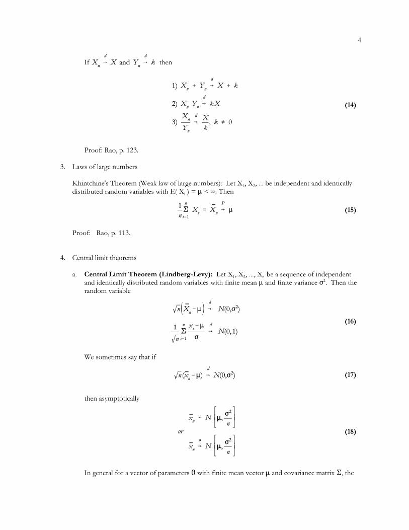
If then

Proof: Rao, p. 123.

3. Laws of large numbers

1 2Khintchine's Theorem (Weak law of large numbers): Let X , X , ... be independent and identically

idistributed random variables with E( X ) = : < 4. Then

Proof: Rao, p. 113.

4. Central limit theorems

1 2 na. Central Limit Theorem (Lindberg-Levy): Let X , X , ..., X be a sequence of independentand identically distributed random variables with finite mean : and finite variance F . Then the2

random variable

We sometimes say that if

then asymptotically

In general for a vector of parameters 2 with finite mean vector : and covariance matrix G, the

5

(19)

(20)

(21)

following holds

We say that is asymptotically normally distributed with mean vector : and covariance matrix(1/n)G.

Proof: Rao, p. 127 or Theil p. 368-9.

1 2 nb. Central Limit Theorem (Lindberg-Feller): Let X , X , ..., X be a sequence of independent

t t t trandom variables. Suppose for every t, X has finite mean : and finite variance F ; Let F be the2

t ndistribution function of X . Define C as follows:

tIf effect, is the variance of the sum of the X . We then consider a condition on “expected

tvalue” of squared difference between X and its expected value

where T is a variable of integration.

Proof: Billingsley, Theorem 27.2 p. 359-61.

1 2c. Multivariate central limit theorem (see Rao: p 128): Let X , X , ... be a sequence of kdimensional vector random variables. Then a necessary and sufficient condition for the

tsequence to converge to a distribution F is that the sequence of scalar random variables 8'Xconverge in distribution for any k-vector 8.

1 2 tCorollary: Let X , X , ... be a sequence of vector random variables. Then if the sequence 8'X

tconverges in distribution to N(0,8'G8) for every 8, the sequence X converges in distribution toN(0,G).

6

(22)

(23)

(24)

(25)

C. Consistency of estimators in the classical linear regression model

1. consistency of

Write the estimator as follows

Consider now the plim of the second term in the product on the right. We will first show that it hasexpected value of zero, and then show that its variance converges to zero.

To determine the variance of write out its definition

Now find the probability limit of this variance

Given that the expected value of is zero and the probability limit of its variance is zero, it

converges in probability to zero, i.e.,

7

(26)

(27)

(28)

(29)

(30)

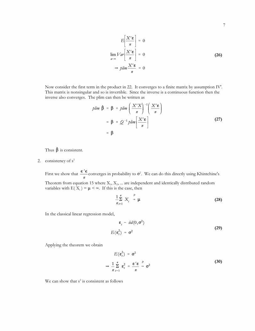
Now consider the first term in the product in 22. It converges to a finite matrix by assumption IV'. This matrix is nonsingular and so is invertible. Since the inverse is a continuous function then theinverse also converges. The plim can then be written as

Thus is consistent.

2. consistency of s2

First we show that converges in probability to F . We can do this directly using Khintchine's2

1 2Theorem from equation 15 where X , X , ... are independent and identically distributed random

ivariables with E( X ) = : < 4. If this is the case, then

In the classical linear regression model,

Applying the theorem we obtain

We can show that s is consistent as follows2

8

(31)

(32)

xNow substitute for M and simplify

9

(33)

(34)

(35)

(36)

(37)

(38)

D. Asymptotic normality of the least squares estimator

1. distribution of

This will converge to the same distribution as

since the inverse is a continuous function and

The problem then is to establish the limiting distribution of

2. asymptotic normality of

Theorem 1: If the elements of g are identically and independently distributed with zero mean and

tifinite variance F , and if the elements of X are uniformly bounded (|X |#R, � t,i), and if2

is finite and nonsingular, then

10

(39)

(40)

(41)

(42)

(43)

Proof (Step 1): Consider first the case where there is only one x variable so that X is a vectorinstead of a matrix. The proof then centers on the limiting distribution of the scalar

t tLet F be the distribution function of g . Note that F does not have a subscript since the g are

t t t tidentically and independently distributed. Let G be the distribution function of x g . G is

tsubscripted because x is different in each time period. Now define a new variable as

Further note that for this simple case Q is defined as

Also note that the central limit theorem can be written in a couple of ways. It can be written in

n n nterms of Z which is a standard normal variable or in terms of V = "Z which has mean zero andvariance " . If a random variable converges to a N(0, 1) variable, then that same random variable2

multiplied by a constant " converges to a N(0, " ) variable. In our case we are interested in the2

t tlimiting distribution of x g . Given that it will have a mean of zero, we are interested in the limiting

t t ndistribution of x g divided by its standard deviation from equation 40. So define Z as follows

n n If we multiply Z by we obtain V as follows

n nSo if we show that Z converges to a standard normal variable, N(0, 1), we have also shown that V

11

(44)

(45)

(46)

(47)

converges to a . Specifically,

Substituting for we obtain

nNow to show that Z converges to N(0, 1), we will apply the Lindberg-Feller theorem on the variable

t tx g which has an expected value of zero. We must use this theorem as opposed to the Lindberg-

t tLevy one because the variance of x g (in equation 40) is not constant over time as x changes. Thetheorem is restated here for convenience.

1 2 nLindberg-Feller Central Limit Theorem – Let X , X , ..., X be a sequence of independent

t t t trandom variables. Suppose for every t, X has finite mean : and finite variance F ; Let F be the2

tdistribution function of X .

where is the variance of the sum of the sequence of random variables considered and is

given by

12

(48)

(49)

(50)

(51)

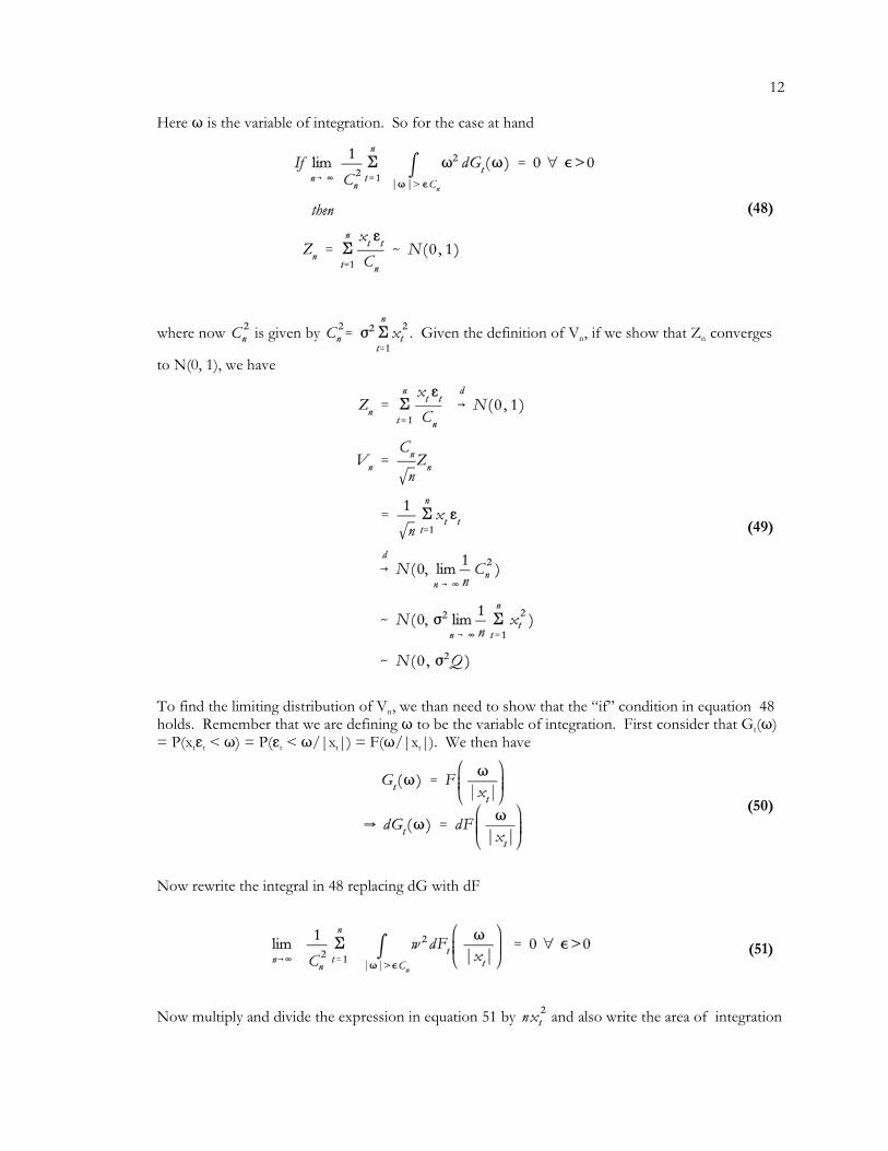
Here T is the variable of integration. So for the case at hand

n nwhere now is given by . Given the definition of V , if we show that Z converges

to N(0, 1), we have

nTo find the limiting distribution of V , we than need to show that the “if” condition in equation 48

tholds. Remember that we are defining T to be the variable of integration. First consider that G (T)

t t t t t= P(x g < T) = P(g < T/|x |) = F(T/|x |). We then have

Now rewrite the integral in 48 replacing dG with dF

Now multiply and divide the expression in equation 51 by and also write the area of integration

13

(52)

(53)

(54)

(55)

(56)

tin terms of the ratio T/x . We divide inside the integral by and then multiply outside the integral

by to obtain

Consider the first part of the expression in equation 52

because and we assume that converges to Q. This expression is finite and

nonzero since it is a sum of squares and the limit is finite by assumption. Now consider the second

t,npart of the expression. Denote the integral by * as follows

Now if we can show that

we are finished because the expression in front from equation 53 converges to a finite non-zero

tconstant. First consider the limit without the x coefficient. Specifically consider

t nThis integral will approach zero as n 6 4 because |x | is bounded and C approaches infinity as napproaches infinity. The point is that the range of integration becomes null as the sample sizeincreases.

14

(57)

(58)

(59)

(60)

(61)

Now consider the fact that

is finite. Because this is finite, when it is multiplied by another term whose limit is zero, the productwill be zero. Thus

The result is then that

Proof (Step 2): We will use the corollary to the multivariate central limit theorem and the abovetheorem. Pick an arbitrary k element vector 8. Consider the variable

The v superscript reminds us that this V is derived from a vector random variable. In effect we are

converting the (kx1) vector variable to a scalar variable. A careful examination of this

shows similarity to equation 39. Comparing them

tthey seem identical except that x is replaced by a summation term . We can now find the

limiting distribution of . First consider its variance.

15

(62)

(63)

(64)

Now consider the limiting distribution of . It will be normal with mean zero and limitingvariance

based on Theorem 1. Now use the corollary to obtain

16

(65)

(66)

(67)

3. asymptotic normality of

Theorem 2: converges in distribution to N(0, F Q )2 -1

Proof: Rewrite as below

Now consider how each term in the product converges.

tNote the similarity of this result to the case when g -N(0, F ) and is distributed as 2

17

(68)

(69)

(70)

(71)

(72)

E. Sufficiency and efficiency in the case of normally distributed errors

1. sufficiency

1 nTheorem: and SSE are jointly sufficient statistics for $ and for F given the sample y , ... , y . To2

show this we use the Neyman-Fisher theorem which we repeat here for convenience.

1 2 nNeyman-Pearson Factorization theorem (jointly sufficient statistics) – Let X , X , ... , X be a

1random sample from the density f(@:2), where 2 may be a vector. A set of statistics T (X) =

1 1 n r 1 n r 1 n 1t (X , ... X ), ... , T (X , ... , X ) = t (X ,...,X ) is jointly sufficient iff the joint distribution of X , ...

n,X can be factored as

1 rwhere g depends on X only through the value of T (X), ..., T (X) and h does not depend on 2and g and h are both nonnegative.

We will show that the joint density can be factored. Specifically we show that

In this case h(y) will equal one. To proceed write the likelihood function, which is also the jointdensity as

Notice that y appears only in the exponent of e. If we can show that this exponent only depends on

and SSE and not directly on y, we have proven sufficiency. Write the sum of squares and then

add and subtract and as follows

The first three terms look very similar to SSE except that the squared term in is missing. Add andsubtract it to obtain

Now substitute from the first order conditions or normal equations the expression for XNy

18

(73)

This expression now depends only on SSE and (the sufficient statistics) and the actual parameter$. Thus the joint density depends only on these statistics and the original parameters $ and F . 2

2. efficiency

Theorem: and s are efficient. 2

Proof: and s are both unbiased estimators and are functions of the sufficient statistics and2

SSE. Therefore they are efficient by the Rao-Blackwell theorem.

19

(74)

(75)

(76)

(77)

F. The Cramer-Rao bounds and least squares

1. The information matrix in the case of normally distributed errors

In order to use the Cramer-Rao theorem we need to validate that the derivative condition holdssince it is critical in defining the information matrix which gives us the lower bound. This derivativecondition is that

where L is the likelihood function. So for our case, first find the derivative of the log likelihoodfunction with respect to $

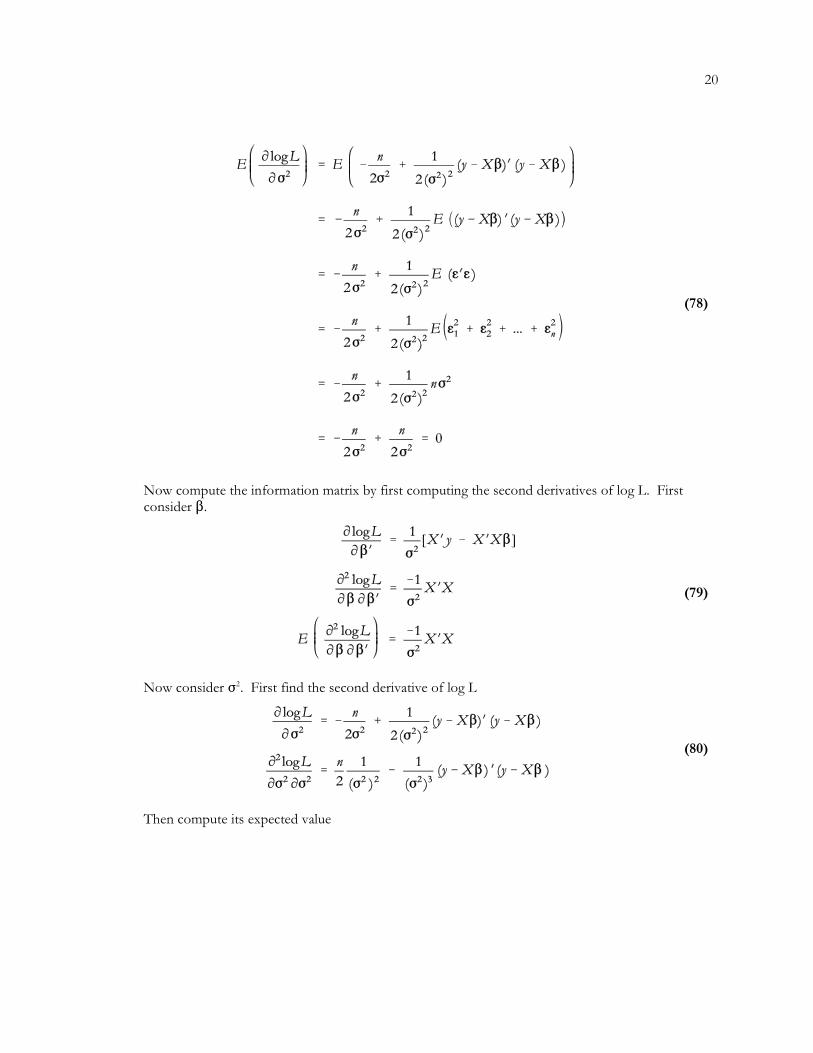
Then find the expected value of this derivative

The condition is satisfied for $, so now find the derivative of the log likelihood function with respectto F .2

Now take the expected value of the log derivative

20

(78)

(79)

(80)

Now compute the information matrix by first computing the second derivatives of log L. Firstconsider $.

Now consider F . First find the second derivative of log L2

Then compute its expected value

21

(81)

(82)

(83)

(84)

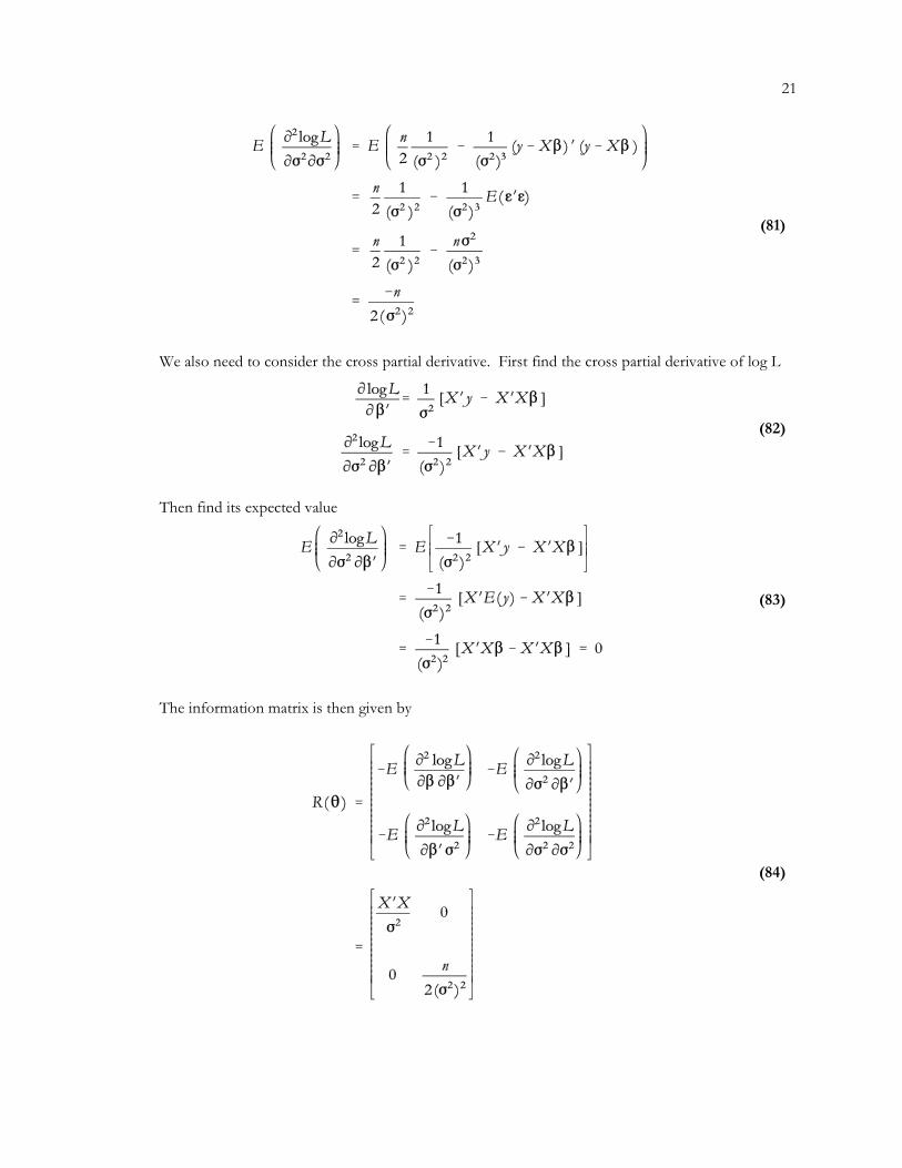
We also need to consider the cross partial derivative. First find the cross partial derivative of log L

Then find its expected value

The information matrix is then given by

22

(85)

(86)

(87)

(88)

This is a diagonal matrix and so its inverse if given by

The covariance matrix of is clearly equal to this lower bound. The sample variance s in the2

classical model has variance which does not reach this bound, but is still efficient as we have

previously shown using the Rao-Blackwell Theorem.

2. Asymptotic efficiency of

Recall that the asymptotic distribution of is N( 0, F Q ). This then implies that the 2 -1

asymptotic variance of is given by (F /n) Q . Consider now the Cramer-Rao lower bound for the2 -1

asymptotic variance. It is given by the appropriate element of

For this element is given by

Thus the asymptotic variance of is equal to the lower bound.

G. Asymptotic distribution of s2

Theorem: Assume that elements of g are iid with zero mean, finite variance F and finite fourth moment2

4: . Also assume that is finite and nonsingular, and that X is uniformly bounded. Then

4the asymptotic distribution of %n(s - F ) is N(0, : - F ). 2 2 4

X xProof: First write SSE = eNe as gNM g as in equation 8. Now consider diagonalizing the matrix M as we

did in determining the distribution of in Theorem 3 on quadratic forms and normal variables.

xSpecifically, diagonalize M using the orthogonal matrix Q as

23

(89)

(90)

(91)

(92)

XBecause M is an idempotent matrix with rank n - k, we know that all its characteristic roots will be zeroor one and that n - k of them will be one. So we can write the columns of Q in an order such that 7 willhave structure

XThe dimension of the identity matrix will be equal to the rank of M , because the number of non-zeroroots is the rank of the matrix. Because the sum of the roots is equal to the trace, the dimension is also

Xequal to the trace of M . Now let w = QNg. Given that Q is orthogonal, we know QNQ = I, that itsinverse is equal to its transpose, i.e., Q = QN, and therefore g = QN w = Qw. Now write out-1 -1

XgNM g/F in terms of w as follows2

Now compute the moments of w,

tIt is useful to also record the moments of the individual w as follows

t t t tSo w is iid with mean zero and variance F just like g . Now define a new variable v = w /F. The2

t texpected value of v is zero and its variance is one. The moments of v and are then given by

24

(93)

(94)

(95)

(96)

t tIn order to compute , we write it in terms of w and g as follows

Substituting equation 94 into equation 93 we obtain

We can then write SSE/F as follows2

What is important is that we have now written SSE in terms of n-k variables, each with mean one and

25

(97)

(98)

(99)

variance C .2

tNow consider the sum from 1 to n-k of the v where we normalize by the standard deviation C and

divide by as follows

This sum converges to a N(0, 1) random variable by the Lindberg-Levy Central Limit Theorem fromequation 16. This can be rearranged as follows

Now substitute in SSE for from equation 96

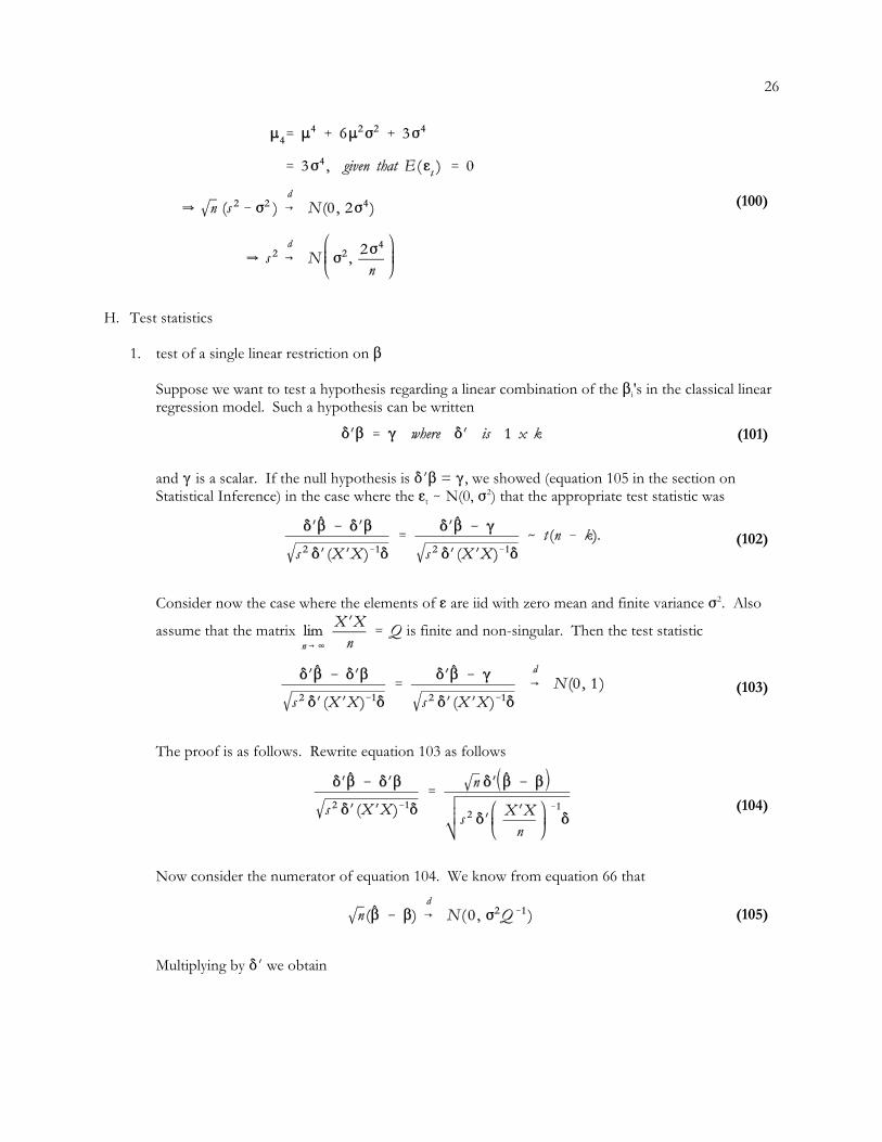
4We showed earlier in the section on review of probability that for a normal distribution, : is given by

26

(100)

(101)

(102)

(103)

(104)

(105)

H. Test statistics

1. test of a single linear restriction on $

iSuppose we want to test a hypothesis regarding a linear combination of the $ 's in the classical linearregression model. Such a hypothesis can be written

and ( is a scalar. If the null hypothesis is *N$ = (, we showed (equation 105 in the section on

tStatistical Inference) in the case where the g - N(0, F ) that the appropriate test statistic was2

Consider now the case where the elements of g are iid with zero mean and finite variance F . Also2

assume that the matrix is finite and non-singular. Then the test statistic

The proof is as follows. Rewrite equation 103 as follows

Now consider the numerator of equation 104. We know from equation 66 that

Multiplying by *N we obtain

27

(106)

(107)

(108)

(109)

Now consider the probability limit of the denominator in equation 104. Note that s converges to F2 2

from equation 32 (i.e., s is a consistent estimator of F ) and by assumption. 2 2

Therefore the denominator converges in probability to

But this is a scalar which is the standard deviation of the asymptotic distribution of the numerator inequation 104 from equation 106. Thus the test statistic equation 103 does converge to a N(0, 1)

variable as can be seen by premultiplying equation 106 by from equation

107.

This test is only asymptotically valid, because in a finite sample the normal distribution is only an

n-kapproximation of the t-distribution. With this in mind, the t distribution can be used in finite

n-ksamples because it converges to N(0, 1). Whether one should use a N(0,1) distribution or a tdistribution in a finite sample is an open question. Note that this result only depended on theconsistency of s , not on its asymptotic distribution from equation 99.2

iTo test the null hypothesis that an individual $ = (, we choose *N to have a one in the ith place andzeroes elsewhere. Given that

from equation 67, we have that

Then using equations 103 and 104 we can see that

28

(110)

(111)

(112)

(113)

The vector *N in this case will pick out the appropriate element of $ and (XNX) .-1

2. test of a several linear restrictions on $

iSuppose we want to test a hypothesis regarding several linear restrictions on the $ 's in the classicallinear regression model. Consider a set of m linear constraints on the coefficients denoted by

We showed in the section on Statistical Inference (equation 109) that we could test such a set ofrestrictions using the test statistic

twhen the g - N(0, F ). Consider now the case where the elements of g are iid with zero mean and2

finite variance F . Also assume that the matrix is finite and non-singular. Then2

under the null hypothesis that R$ = r, the test statistic

We can prove this by finding the asymptotic distribution of the numerator, given that thedenominator of the test statistic is s which is a consistent estimator of F . We will attempt to write2 2

the numerator in terms of g. First write as a function of ,

29

(114)

(115)

(116)

(117)

(118)

Then write out the numerator of equation 113 as follows

This is the same expression as in equation 112 of the section on Statistical Inference. Notice byinspection that the matrix S is symmetric. We showed there that it is also idempotent. We canshow the trace is as follows using the property of the trace that trace (ABC) = trace (CAB) = trace(BCA)

Given that S is idempotent, its rank is equal to its trace. Now consider diagonalizing S using anorthogonal matrix Q as we did in equation 89, that is find the normalized eigenvectors of S anddiagonalize as follows

The dimension of the identity matrix is equal to the rank of S, because the number of non-zeroroots is the rank of the matrix. Because the sum of the roots is equal to the trace, the dimension isalso equal to the trace of S. Now let v = QNg/F. Given that Q is orthogonal, we know that itsinverse is equal to its transpose, i.e., Q = QN and therefore g = QN Fv = QFv. Furthermore QQN-1 -1

n= I because Q is orthogonal. We can then write

30

(119)

(120)

(121)

Substituting in from equation 117 we then obtain

Now compute the moments of v,

The test statistic in equation 113 then has a distribution of . This is the sum of the squares

iof an iid variable. If we can show that v is distributed asymptotically normal, then this sum will

idistributed P . So we need to find the asymptotic distribution of v . To do this, it is helpful to write2

out the equation defining v as follows

31

(122)

(123)

(124)

(125)

(126)

iWe then can write v as

The expected value and variance of each term in the summation is computed as

iwhere each of the terms in the sum is independent. The variance of v is given by

iThe variance of v is obtained by the inner product of the ith row of QN with the ith column of Q. Given that Q is orthogonal, this sum of squares is equal to one. Now let F be the distribution

tfunction of g as before in the proof of asymptotic normality the least squares estimator. And in this

t ti tcase, let G be the distribution function of Q g /F. Define as

inNow define Z as follows

in iSo if we show that Z converges to a standard normal variable, N(0, 1), we have also shown that v

32

(127)

(128)

(129)

(130)

inconverges to N(0, 1). To show that Z converges to N(0, 1), we will apply the Lindberg-Feller

ti ttheorem on the variable Q g /F which has an expected value of zero. The theorem we remember isas follows.

1 2 nLindberg-Feller Central Limit Theorem – Let X , X , ..., X be a sequence of independent

t t t trandom variables. Suppose for every t, X has finite mean : and finite variance F ; Let F be the2

tdistribution function of X .

where is the variance of the sum of the sequence of random variables.

t1 1 t2 2 t3 3 tn nThe elements of sequence for this case are Q g /F, Q g /F, Q g /F, . . . Q g /F. The mean of

each variable is zero. The variance of the ith term is , which is finite. If the Lindberg condition

holds, then

The proof we gave previously that the Lindberg condition holds is valid here given that we are

t t tsimply multiplying g by a constant in each time period ( = , which is analogous to x in the

previous proof. Given that

then

In finite samples, the P (m)/m distribution is an approximation of the actual distribution of the test2

statistic. One can also use an F (m, n-k) distribution because it converges to a P (m)/m distribution2

as n 6 4. This is the case because P (m)/m 61 as m 6 4. We can show this as follows by noting2

that E(P (m)) = m and Var (P (m) ) = 2m. Consider then that2 2

33

(131)

(132)

(133)

Now remember that Chebyshev’s inequality implies that

Applying it to this case we obtain

As m 6 4, . Thus, the usual F tests used for multiple restrictions on the coefficient

tvector $ are asymptotically justified even if g is not normally distributed, as long as g -iid(0, F ).2

34

Some References

Amemiya, T. Advanced Econometrics. Cambridge: Harvard University Press, 1985.

Bickel, P.J. and K.A. Doksum. Mathematical Statistics: Basic Ideas and Selected Topics, Vol 1). 2 Edition. nd

Upper Saddle River, NJ: Prentice Hall, 2001.

Billingsley, P. Probability and Measure. 3rd edition. New York: Wiley, 1995.

Casella, G. And R.L. Berger. Statistical Inference. Pacific Grove, CA: Duxbury, 2002.

Cramer, H. Mathematical Methods of Statistics. Princeton: Princeton University Press, 1946.

Goldberger, A.S. Econometric Theory. New York: Wiley, 1964.

Rao, C.R. Linear Statistical Inference and its Applications. 2nd edition. New York: Wiley, 1973.

Schmidt, P. Econometrics. New York: Marcel Dekker, 1976

Theil, H. Principles of Econometrics. New York: Wiley, 1971.

35

(134)

(135)

(136)

We showed previously that

A P variable is the sum of squares of independent standard normal variables. The degrees of2

freedom is the number of terms in the sum. This means that we can write the expression as where

teach of the variables v is a standard normal variable with mean zero and variance one. The square

tof v is a P variable with one degree of freedom. The mean of a P variable is the degrees of2 2

freedom and the variance is twice the degrees of freedom. (See the statistical review.) Thus thevariable has mean 1 and variance 2. The Lindberg-Levy version of the Central Limit theoremgives for this problem

This can be rearranged as follows