small sample performance of dynamic panel data estimators...

Small Sample Performance of Dynamic Panel DataEstimators: A Monte Carlo Study on the Basis of

Growth Data

Nazrul IslamDepartment of Economics

Emory University

Current Draft: August, 1998

---------------------------------------------------------------------Initial versions of this paper were presented in seminars at Harvard University and

Emory University. I would like to thank the participants of these seminars whose commentshelped improve this paper. All remaining errors are mine.

1

Small Sample Performance of Dynamic Panel DataEstimators: A Monte Carlo Study on the Basis of Growth

Data

1. Introduction

This paper investigates the small sample properties of dynamic panel data estimators

as applied for estimation of growth-convergence equation using Summers-Heston (1988,

1991) data set. It shows that, among various estimators used for this purpose, the ones not

using lagged dependent variable as instrument perform better than the ones that do. This is

an important result, which is useful in assessing the results on convergence equation

presented recently by different authors using different dynamic panel data estimators.

One of the issues around which new growth literature has evolved is that of

convergence. Statistically, convergence has been interpreted as a negative correlation

between initial level of income and subsequent growth rate. Hence, the popular method for

testing convergence hypothesis has been to conduct growth-initial level regressions. For a

long time, these regressions were estimated using cross-section data only. However, in the

early nineties, it was observed that the cross-section approach suffers from certain important

limitations in this regard. This led to the panel approach, and since then use of panel data in

estimating the convergence equation has become quite common

Close scrutiny show that the growth-initial level regression is actually a dynamic

panel data model. This provides the rationale for using dynamic panel data estimators. The

resulting panel estimates generally differ from the cross-section estimates. However, they

also differ among themselves. This poses a problem because the properties of the dynamic

panel data estimators are mostly asymptotic, and hence, their small sample properties are a-

priori not known. It is therefore difficult to judge which of the different panel estimates are

more reasonable.

The Monte Carlo study presented in this paper is a response to this difficulty. It is

customized to the data set and specification that are generally used in growth and

convergence studies. The estimators included in this study are the instrumental variable (IV)

estimators of Anderson and Hsiao (1981, 1982), the multivariate estimators, including the

Minimum Distance estimator, suggested by Chamberlain (1982, 1983), and the generalized

2

method of moments (GMM) estimators proposed by Arellano (1989a, 1989b) and Arellano

and Bond (1991). In addition, we also include conventional estimators like the ordinary least

squares (OLS), least squares with dummy variable (LSDV), and a few other simultaneous

equations estimators.

Two things emerge from this exercise. First, wide variation is actually observed in

the results from different dynamic panel estimators. Second, estimators that rely on further

lagged values of the dependent variable as instruments perform worse than the estimators

that do not rely on them as instruments. These two results together suggest that significant

caution should accompany presentation of results from specific panel estimator. In fact, it

seems desirable that researchers check out the reliability of their panel results by conducting

their own Monte Carlo experiments.

2. Previous Monte Carlo Studies

The issue of small sample properties of dynamic panel data estimators is not entirely

new. There have been earlier attempts to investigate it. For example, Nerlove (1967)

considers a simple auto-regressive model with no exogenous variable, and compares the

performance of OLS, LSDV, MLE, and several variants of GLS in estimating the model. In

Nerlove (1971), the dynamic panel data model is extended to have exogenous variable. This

allows consideration of instrumental variable (IV) estimator with lagged values of the

exogenous variable as instrument. It also allows having another variant of two-stage GLS.

Overall, Nerlove’s Monte Carlo results favor GLS estimators over other estimators.

Since Nerlove’s work, there have been significant developments in the field of

dynamic panel data estimators. Among these has been introduction of Anderson and Hsiao

IV estimators which use further lagged values of the dependent variable as instruments.

Arellano has carried this idea forward and has proposed using all possible further lagged

variables as instruments within a GMM framework. Arellano and Bond (1991) perform a

Monte Carlo study to compare primarily the small sample properties of their GMM

estimators with the corresponding properties of Anderson-Hsiao estimators. According to

their results, the GMM estimators perform better than Anderson-Hsiao IV estimators though

not so much in terms of bias as in terms of dispersion.

3

3. Objectives of the Present Study

Given these earlier studies, what can be the motivation for the Monte Carlo study

presented in this paper? There are several of them. First, Monte Carlo results have been

generally found to be more useful when these are customized to the particular model, data

set, and range of parameter values that pertain to the actual problem to which application of

panel data estimators is being considered. Thus, in view of the controversy regarding

convergence parameter estimates, it is useful to have Monte Carlo results that are specific to

the growth-convergence equation, specific to the Summers-Heston growth data set, and

specific to the pertinent range of parameter values. This is exactly what is done in this

exercise. This also leads to the following second motivation. The previous Monte Carlo

studies have generally focussed on panel data models with random individual effects.

However, the individual effect that arises in the growth-convergence equation is of

correlated nature. There have been no Monte Carlo results, as far as we know, on models

with correlated effects. The third motivation for this study arises from the fact that several

important dynamic panel estimators do not find place in the earlier Monte Carlo studies.

Among these are the estimators that use the multivariate approach, like the three stage least

squares (3SLS) and generalized three stage least squares (G3SLS). In addition,

Chamberlain’s MD estimator also remains outside the purview of the previous Monte Carlo

studies. The MD estimator using optimal weighting matrix, sometimes referred to as

Optimal Minimum Distance Estimator (OMDE), has been used as the benchmark for

judging theoretical efficiency of many of the GMM estimators proposed by Arellano. So it is

of some interest that Monte Carlo study covered these estimators as well. The present study

takes a comprehensive view and includes almost all the known dynamic panel data

estimators for evaluation. Fourth, the present study does not limit itself to only one

particular generating mechanism of the transitory error term. Instead, it considers three

different generating schemes are considered, namely uncorrelated, autoregressive, and

moving average. Finally, the study also investigates the impact of sample size on relative

performance of the estimators. This is very relevant for the problem at hand. The

convergence equation has generally been estimated in the context of two different samples

of countries, one being small and the other, large. It is therefore necessary to see how

different estimators perform in these samples of different size.

4

Model and Parameter Values

The Model

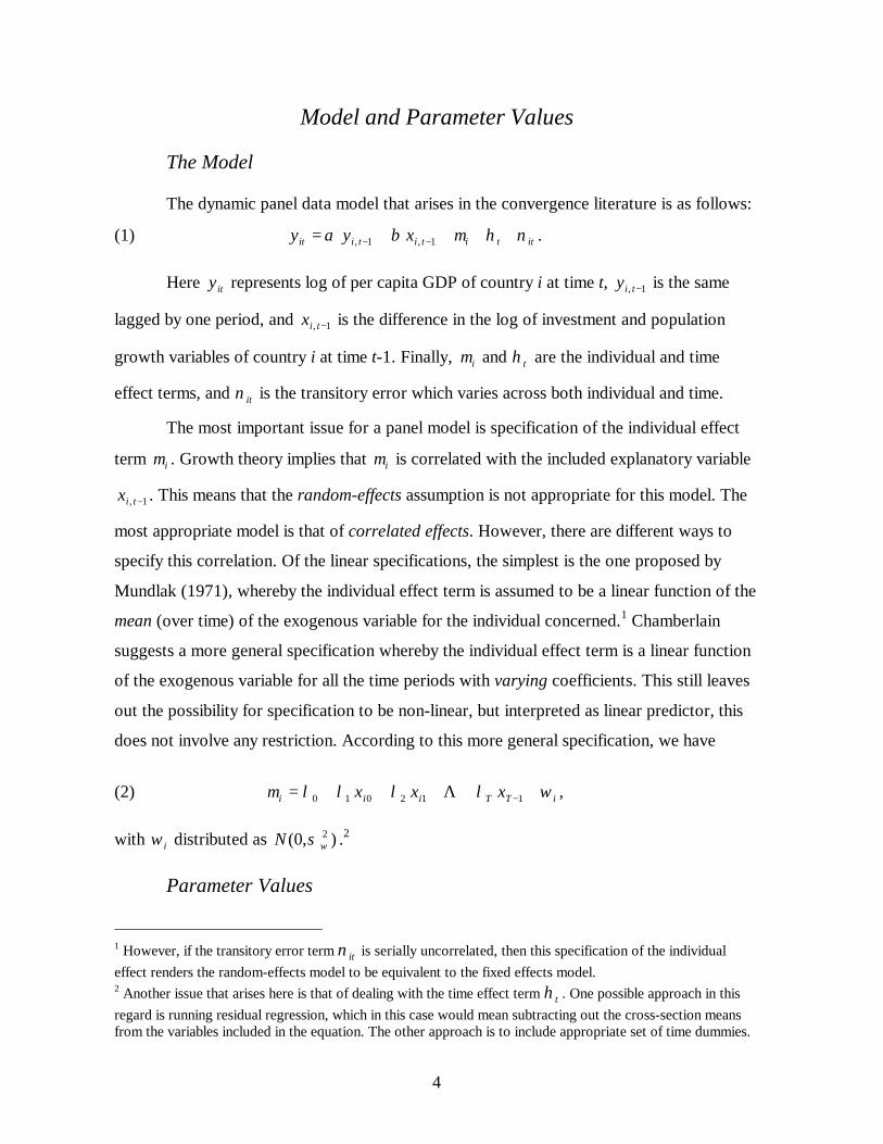
The dynamic panel data model that arises in the convergence literature is as follows:

(1) ittititiit xyy νηµβα ++++= −− 1,1, .

Here ity represents log of per capita GDP of country i at time t, 1, −tiy is the same

lagged by one period, and 1, −tix is the difference in the log of investment and population

growth variables of country i at time t-1. Finally, iµ and tη are the individual and time

effect terms, and itν is the transitory error which varies across both individual and time.

The most important issue for a panel model is specification of the individual effect

term iµ . Growth theory implies that iµ is correlated with the included explanatory variable

1, −tix . This means that the random-effects assumption is not appropriate for this model. The

most appropriate model is that of correlated effects. However, there are different ways to

specify this correlation. Of the linear specifications, the simplest is the one proposed by

Mundlak (1971), whereby the individual effect term is assumed to be a linear function of the

mean (over time) of the exogenous variable for the individual concerned.1 Chamberlain

suggests a more general specification whereby the individual effect term is a linear function

of the exogenous variable for all the time periods with varying coefficients. This still leaves

out the possibility for specification to be non-linear, but interpreted as linear predictor, this

does not involve any restriction. According to this more general specification, we have

(2) iTTiii xxx ωλλλλµ +++++= − 112010 Λ ,

with iω distributed as ),0( 2ωσN .2

Parameter Values

1 However, if the transitory error term itν is serially uncorrelated, then this specification of the individualeffect renders the random-effects model to be equivalent to the fixed effects model.2 Another issue that arises here is that of dealing with the time effect term tη . One possible approach in thisregard is running residual regression, which in this case would mean subtracting out the cross-section meansfrom the variables included in the equation. The other approach is to include appropriate set of time dummies.

5

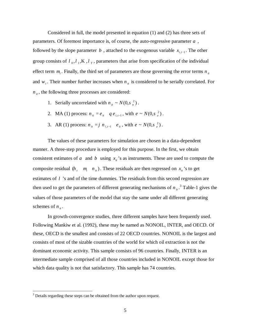
Considered in full, the model presented in equation (1) and (2) has three sets of

parameters. Of foremost importance is, of course, the auto-regressive parameter α ,

followed by the slope parameter β , attached to the exogenous variable 1, −tix . The other

group consists of Tλλλ ,,, 10 Κ , parameters that arise from specification of the individual

effect term iµ . Finally, the third set of parameters are those governing the error terms itν

and iω . Their number further increases when itν is considered to be serially correlated. For

itν , the following three processes are considered:

1. Serially uncorrelated with ),0(~ 2νσν Nit .

2. MA (1) process: 1, −+= tiitit εθεν , with ),0(~ 2εσε N .

3. AR (1) process: ittiit ενϕν += − 1, , with ),0(~ 2εσε N .

The values of these parameters for simulation are chosen in a data-dependent

manner. A three-step procedure is employed for this purpose. In the first, we obtain

consistent estimates of α and β using itx ’s as instruments. These are used to compute the

composite residual )( itit νµη ++ . These residuals are then regressed on itx ’s to get

estimates of λ’s and of the time dummies. The residuals from this second regression are

then used to get the parameters of different generating mechanisms of itν .3 Table-1 gives the

values of those parameters of the model that stay the same under all different generating

schemes of itν .

In growth-convergence studies, three different samples have been frequently used.

Following Mankiw et al. (1992), these may be named as NONOIL, INTER, and OECD. Of

these, OECD is the smallest and consists of 22 OECD countries. NONOIL is the largest and

consists of most of the sizable countries of the world for which oil extraction is not the

dominant economic activity. This sample consists of 96 countries. Finally, INTER is an

intermediate sample comprised of all those countries included in NONOIL except those for

which data quality is not that satisfactory. This sample has 74 countries.

3 Details regarding these steps can be obtained from the author upon request.

6

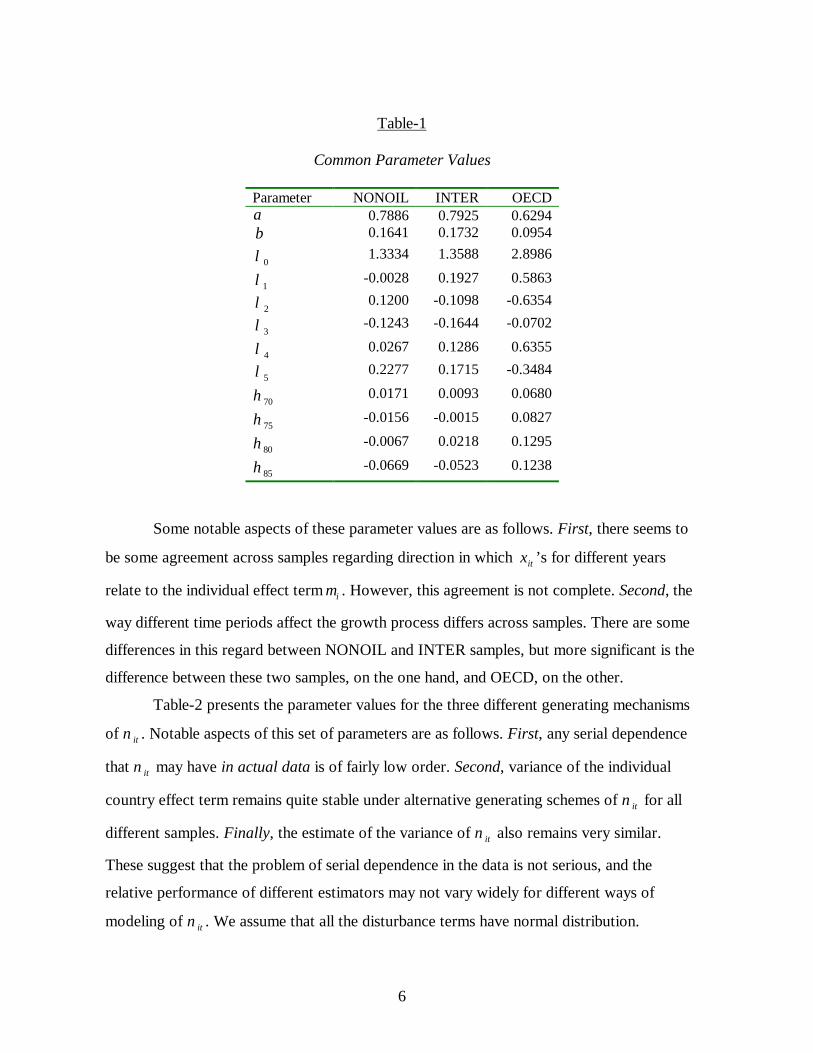
Table-1

Common Parameter Values

Parameter NONOIL INTER OECDα 0.7886 0.7925 0.6294β 0.1641 0.1732 0.0954

0λ 1.3334 1.3588 2.8986

1λ -0.0028 0.1927 0.5863

2λ 0.1200 -0.1098 -0.6354

3λ -0.1243 -0.1644 -0.0702

4λ 0.0267 0.1286 0.6355

5λ 0.2277 0.1715 -0.3484

70η 0.0171 0.0093 0.0680

75η -0.0156 -0.0015 0.0827

80η -0.0067 0.0218 0.1295

85η -0.0669 -0.0523 0.1238

Some notable aspects of these parameter values are as follows. First, there seems to

be some agreement across samples regarding direction in which itx ’s for different years

relate to the individual effect term iµ . However, this agreement is not complete. Second, the

way different time periods affect the growth process differs across samples. There are some

differences in this regard between NONOIL and INTER samples, but more significant is the

difference between these two samples, on the one hand, and OECD, on the other.

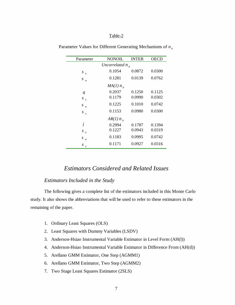
Table-2 presents the parameter values for the three different generating mechanisms

of itν . Notable aspects of this set of parameters are as follows. First, any serial dependence

that itν may have in actual data is of fairly low order. Second, variance of the individual

country effect term remains quite stable under alternative generating schemes of itν for all

different samples. Finally, the estimate of the variance of itν also remains very similar.

These suggest that the problem of serial dependence in the data is not serious, and the

relative performance of different estimators may not vary widely for different ways of

modeling of itν . We assume that all the disturbance terms have normal distribution.

7

Table-2

Parameter Values for Different Generating Mechanisms of itν

Parameter NONOIL INTER OECDUncorrelated itν

νσ 0.1054 0.0872 0.0300

ωσ 0.1281 0.0139 0.0762

MA(1) itνθ 0.2037 0.1250 0.1125

νσ 0.1179 0.0990 0.0302

ωσ 0.1225 0.1010 0.0742

εσ 0.1153 0.0980 0.0300

AR(1) itνϕ 0.2994 0.1787 0.1394

νσ 0.1227 0.0943 0.0319

ωσ 0.1183 0.0995 0.0742

εσ 0.1171 0.0927 0.0316

Estimators Considered and Related Issues

Estimators Included in the Study

The following gives a complete list of the estimators included in this Monte Carlo

study. It also shows the abbreviations that will be used to refer to these estimators in the

remaining of the paper.

1. Ordinary Least Squares (OLS)

2. Least Squares with Dummy Variables (LSDV)

3. Anderson-Hsiao Instrumental Variable Estimator in Level Form (AH(l))

4. Anderson-Hsiao Instrumental Variable Estimator in Difference From (AH(d))

5. Arellano GMM Estimator, One Step (AGMM1)

6. Arellano GMM Estimator, Two Step (AGMM2)

7. Two Stage Least Squares Estimator (2SLS)

8

8. Three Stage Least Squares Estimator (3SLS)

9. Generalized Three Stage Least Squares Estimator (G3SLS)

10. Minimum Distance Estimator (MD)

Brief description of these estimators, as applied to the model considered in this

study, is provided in Appendix. We can, therefore, directly proceed to presentation of the

Monte Carlo work.

Sample Size and Related Issues:

Given a certain number of cross-sections available (i.e., given T), different panel data

estimators can make use of different numbers of these in the final stage of estimation. In

simulation, therefore, it is possible to adopt two different approaches. First, it is possible to

keep the actual number of cross-sections used by the estimators the same by generating

varying number of cross-sections for different estimators. Second, the number of cross-

sections generated may be kept the same, and the number of actual cross-sections used in the

final stage of estimation by different estimators may be allowed to vary. It is the second

situation that a researcher faces in actual practice. She confronts a given data set and then

has to choose from among different estimators depending on their relative merits. In order to

conform to this real situation, this study adopts the second approach. This also conforms to

the fact that this Monte Carlo study is based on a given data set, namely Summers-Heston

growth data set. The panel based on this data set is considered at five-year intervals. Thus,

the data available are for 1960, 1965, 1970, 1975, 1980, and 1985. Since this is a dynamic

model as given by equation (1), the effective T equals to five.

Issues Particular to Individual Estimators

OLS:

OLS, the simplest of all estimators considered, is applied to the equation in the level

form. Since initial values of ity (i.e., of 1960) are known, OLS can use in actual estimation

all of the T cross-sections. OLS, however, is not geared to providing estimates of either tλ’s

or iµ ’s. It gives an estimate of the composite error term itu but cannot provide its further

9

decomposition into the component parts, iµ and itν . Also, OLS is inconsistent even with T

going to infinity.

LSDV:

LSDV is also applied to the equation in level form and, for the same reasons as with

OLS, all of the T cross-sections can be used in actual estimation. It can provide estimates of

iµ ’s (viewed as parameters to be estimated) and hence of tλ’s, from a subsequent

regression of the estimated iµ on the itx s. Also, it can give estimates of variances of the

two error components separately. The between-group variations or, more directly, variance

of the estimated iµ ’s, can be used to get an estimate of 2µσ . On the other hand, 2

vσ may be

obtained from the within-group variations. LSDV estimator, though not consistent in the

direction of N, is consistent when T goes to infinity.

AH(l) and AH(d):

Both these IV estimators apply to the model in first-differenced form. This results in

the ‘loss’ of one cross-section from the actual estimation exercise. Furthermore, since in

AH(l) 2, −tiy is used as instrument for )( 2,1, −− − titi yy , one more cross-section is lost in the

process. Thus, if T cross-sections are available, the number of cross-sections actually used is

(T-2). AH(l) is mainly geared to consistent estimation of the slope parameters α and β . It

can also provide an estimate of 2νσ . However, other parameters of the model cannot be

recovered using this estimator. AH(d) has similar features as those of AH(l). However, since

AH(d) uses )( 3,2, −− − titi yy as instrument for )( 2,1, −− − titi yy , two cross-sections are lost in

the process. Hence with T cross-sections available, only (T-3) are used. When T is small, this

may be an important consideration.

AGMM(1) and AGMM(2):

Like the AH estimators, both AGMM(1) and AGMM(2) work with the model in first

differenced form. This results in loss of one cross-section from the actual estimation process.

AGMM(1) is based on arbitrary weighting matrix, whereas in AGMM(2) the weighting

matrix is appropriately constructed using residuals from AGMM1 estimation. The details of

10

the construction of the instrument matrix have been sketched in Appendix. Like AH

estimators, these estimators are also geared to estimation of α and β , and do not provide

estimates of the remaining parameters.

2SLS, 3SLS, and G3SLS:

This set of estimators may be commonly referred to as Simultaneous Equation (SE)

estimators. All of them apply to the model in first differenced form. Thus, if T is the number

of cross-sections available, the number of equations used in estimation is (T-1). These

estimators are also geared to estimation of α and β .4 One issue in G3SLS estimation is

which residuals to use for construction of the covariance matrix. The residuals can be

obtained from either 2SLS or 3SLS or even from a generalized 2SLS. However, this does

not change the asymptotic properties of the estimator. In this study residuals from 2SLS are

used for both 3SLS and G3SLS.

MD:

In contrast with AH, AGMM, and SE estimators, MD works with the model in

levels. Hence, all the cross-sections available can be used in estimation. Instead of

eliminating iµ through first differencing, as other estimators do, MD specifies iµ in terms

of its correlation with itx ’s, and uses this specification to substitute for iµ . Hence, his

estimator can provide estimates not only of the slope parameters of the main dynamic

equation but also of the tλ’s. However, this also makes MD a non-linear estimation

procedure. An important issue in MD estimation, therefore, is of setting initial values of the

parameters for non-linear iteration to proceed. The task is made difficult by the fact that, in

case of a simulation exercise, the true parameter values are known! A related question is

whether to use the same set of initial values to start the iteration for each replication or to

change it over replications. In this study, we resolve these issues in the following manner.

4 However, in principle it is possible to add the equation for iµ to the system. This raises the number of

equations to T and allows having estimates of tλ ’s. However, inclusion of the equation for iµ into the system

does not affect the asymptotic properties of the estimates of α and β because there are no across-equation

restrictions between the equation for iµ and those for ty ’s.

11

It is impossible to set ‘arbitrary’ initial values that are free from prior knowledge of

the true parameter values because they are known! Hence, it is preferable to have these

initial values result from a routine, for example, from a preliminary estimation procedure.

This also resolves the other question and allows the initial values to be data-dependent and

hence be different across replications. However, the question that arises is, which particular

estimator to use for generating the initial parameter values? It is clear that LSDV is the most

likely candidate because it is the only estimator other than MD that provides estimates of not

onlyα and β but also of the tλ s.

In MD estimation, there is also the issue of choosing the weighting matrix. There are

several options in this regard and the optimality of the estimates depends on the choice. This

study uses the optimal weighting matrix, which takes full account of possible

heteroskedasticity across individuals.

Simulation Results and Discussion

It is apparent from the discussion above that not all the panel estimators are geared to

provide estimate all the parameters of the model. Because of this and also in order not to

clutter the presentation with too many numerical results, we focus here on results concerning

only α and β , the main parameters of the model.5 The simulation results presented in this

paper are on the basis of one thousand replications. In most cases, Monte Carlo distributions

stabilized already with one hundred replications. Hence increasing the number of

replications by any further was not necessary.

The detailed results regarding the Monte Carlo distributions obtained from the study

are provided in three sets of tables in the Appendix for three different generating

mechanisms of itν . Tables A1 to A3 show results for different samples when itν is serially

uncorrelated. Similarly, Tables A4 to A6 give results when itν follows an MR(1) process.

Finally, Tables A7 to A9 give results when itν obeys an AR(1) scheme.

The two criteria that are usually used in judging performance of an estimator are bias

and mean square error (MSE). In order to make assessment of performance of the estimators

5 Hence, we do not report the results regarding the error variances.

12

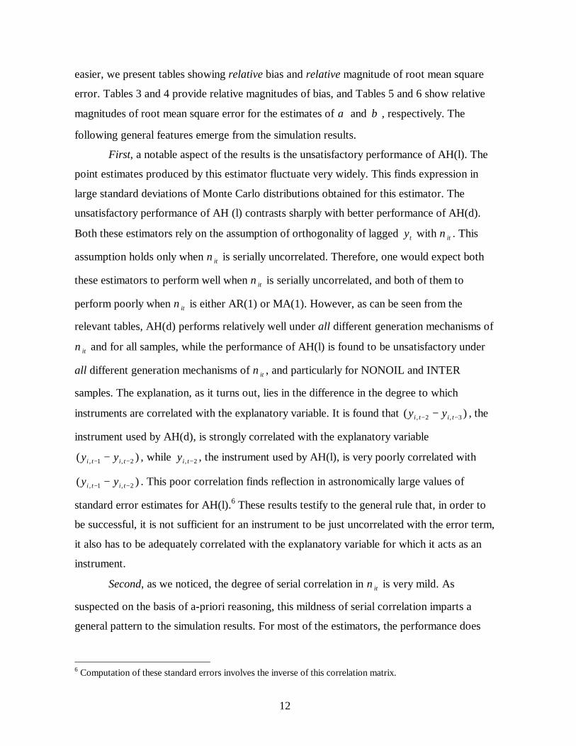
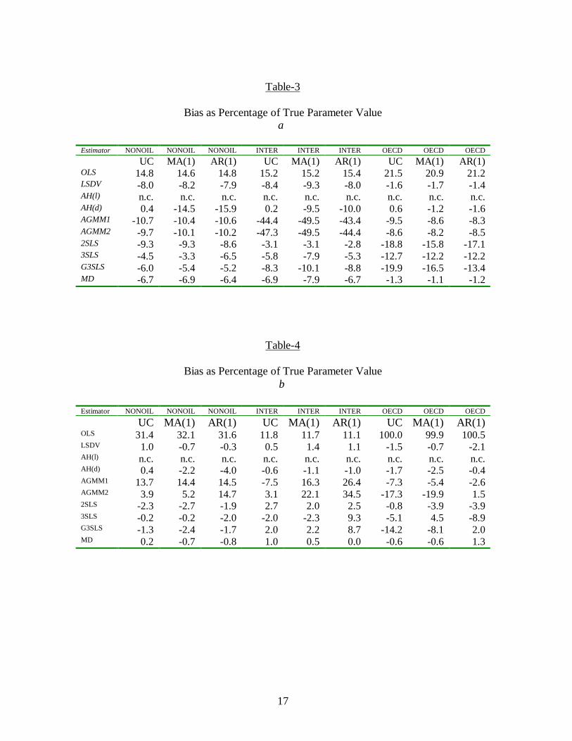
easier, we present tables showing relative bias and relative magnitude of root mean square

error. Tables 3 and 4 provide relative magnitudes of bias, and Tables 5 and 6 show relative

magnitudes of root mean square error for the estimates of α and β , respectively. The

following general features emerge from the simulation results.

First, a notable aspect of the results is the unsatisfactory performance of AH(l). The

point estimates produced by this estimator fluctuate very widely. This finds expression in

large standard deviations of Monte Carlo distributions obtained for this estimator. The

unsatisfactory performance of AH (l) contrasts sharply with better performance of AH(d).

Both these estimators rely on the assumption of orthogonality of lagged ty with itν . This

assumption holds only when itν is serially uncorrelated. Therefore, one would expect both

these estimators to perform well when itν is serially uncorrelated, and both of them to

perform poorly when itν is either AR(1) or MA(1). However, as can be seen from the

relevant tables, AH(d) performs relatively well under all different generation mechanisms of

itν and for all samples, while the performance of AH(l) is found to be unsatisfactory under

all different generation mechanisms of itν , and particularly for NONOIL and INTER

samples. The explanation, as it turns out, lies in the difference in the degree to which

instruments are correlated with the explanatory variable. It is found that )( 3,2, −− − titi yy , the

instrument used by AH(d), is strongly correlated with the explanatory variable

)( 2,1, −− − titi yy , while 2, −tiy , the instrument used by AH(l), is very poorly correlated with

)( 2,1, −− − titi yy . This poor correlation finds reflection in astronomically large values of

standard error estimates for AH(l).6 These results testify to the general rule that, in order to

be successful, it is not sufficient for an instrument to be just uncorrelated with the error term,

it also has to be adequately correlated with the explanatory variable for which it acts as an

instrument.

Second, as we noticed, the degree of serial correlation in itν is very mild. As

suspected on the basis of a-priori reasoning, this mildness of serial correlation imparts a

general pattern to the simulation results. For most of the estimators, the performance does

6 Computation of these standard errors involves the inverse of this correlation matrix.

13

not vary to a great extent with respect to the alternative generating scheme of itν . We have

already seen this in the context of the AH estimators. Going by the results on α , this is true

even for AGMM1 and AGMM2. This is somewhat surprising because these estimators

depend rather heavily for their validity on orthogonality of lagged values of ity to itν , and

this orthogonality is violated when itν follows either an AR or a MA scheme.7

Third, performance of many of the estimators shows considerable variation with

respect to the sample considered. However, it is difficult to establish a single pattern in this

regard. For example, going by the results on bias of estimated α , performance of OLS

deteriorates for OECD when compared with that for either NONOIL or INTER samples.

However, in case of LSDV and MD, the opposite is true. The AGMM and SEM estimators

show yet a different kind of contrast. The performance of the AGMM estimators deteriorates

for INTER sample in comparison with that for either NONOIL or OECD. In case of SEM

estimators, the opposite is true. The contrasting performance of AGMM and SEM estimators

may not be entirely surprising in view of the fact that while the former depends on lagged

ity ’s as instruments, SEM estimators rely entirely on itx ’s.

Fourth, comparison of the performance of 3SLS and G3SLS with that of 2SLS

yields mixed results. In the NONOIL sample, regardless of generating mechanism for itν ,

results from 3SLS and G3SLS estimators seem to be better than that from 2SLS. For INTER

sample, however, 2SLS seems to perform better than either 3SLS or G3SLS. In case of the

OECD sample, the situation is less clear cut. In terms of mean of the Monte Carlo

distribution, 3SLS and G3SLS fare better than 2SLS, though not in terms of dispersion. On

the other hand, in the OECD sample, the Monte Carlo distributions for 2SLS have very large

standard deviation.

One reason for deterioration of performance of 3SLS and G3SLS estimators in

INTER and OECD samples, when compared to that in NONOIL sample, may lie in sample-

size. The sizes of INTER and OECD samples are smaller that that of NONOIL. Since the

7 To be accurate, it needs to be mentioned that AH(d) does show some expected sensitivity with respect to thegeneration scheme of itν . Why similar sensitivity is not found in the performance of the AGMM estimators isan interesting question.

14

superiority of 3SLS and G3SLS over 2SLS is an asymptotic result, a larger sample size may

help this result to surface.

Fifth, the MD estimator performs better in comparison with AGMM estimators. With

regard to α , this is particularly true for INTER and OECD samples. For β this is true for

all different samples. In terms of bias, some of the SEM estimators perform slightly better

than MD in some of the samples. Thus, for example, with regard to α , 3SLS and G3SLS

show less bias than MD in NONOIL and INTER samples. However, in case of OECD, the

bias involved with the former estimators is much larger than with the latter. Regarding β ,

MD estimator shows less bias than by SEM estimators for INTER sample as well. Even for

the NONOIL sample, the bias involved with the MD is similar to and sometimes less than

that with SEM estimators.

Bias of the Monte Carlo distributions needs to be evaluated in conjunction with

corresponding dispersion. Mean Square Error (MSE) is the popular measure that is used to

take into account the possible trade-off between bias and variance. Looking at the values of

root MSE (presented in Tables 5 and 6) of Monte Carlo distribution of the parameter

estimates, we see that the MD estimator proves to be uniformly superior to AGMM and

SEM estimators. The only exception in this regard is the performance of 2SLS in estimating

β in the INTER sample. We earlier noted somewhat erratic performance of AH(d). In terms

of bias, it performs better than MD in some isolated cases. However, in terms of root MSE,

except for one lone exception, MD outperforms AH(d).

Thus, overall, among the N-consistent estimators, MD appears to be a more

dependable estimator for estimating the growth convergence equation using Summers-

Heston data set. One problem noticed with MD estimator for the problem at hand is its

sensitivity with respect to the starting values of iteration procedure. However, in case of a

single estimation exercise, it is possible to explore this sensitivity by looking at the

minimum distance statistic of the converged results obtained from different starting values.

Applying this procedure, it can be ensured that a global maximum is reached, and not a local

one.

One surprising aspect of the results was the relatively better performance of LSDV.

In terms of both bias and root MSE, and in estimation of both α and β , LSDV proves to be

a relatively superior estimator for the problem at hand. This is somewhat surprising given

15

that theoretically LSDV is consistent only in the direction of T, and the data used in this

study has a small T. What this shows is that small sample properties of estimators may be

very specific to the model and data considered.

From another point of view, it is also interesting to note that simpler estimators such

as LSDV and 2SLS (and in some cases, AH(d)) outperform more sophisticated estimators

such as AGMM2 and some of the SEM estimators. This helps draw attention to the

following important fact. The optimal properties of sophisticated estimators often depend on

use of optimal weighting matrix. Unfortunately however, these weighting matrices have to

be estimated, and as a result, they pick up, along with signal, noise present in the data. This

noise gets transmitted to the final parameter estimates when these are produced using the

estimated weighting matrices. To the extent that simpler estimators do not have to use

estimated weighting matrices, they are spared of this potential source of additional noise.

This explains why sophisticated estimators may actually perform worse than simpler

estimators, though this does not necessarily have to be the case.

Conclusions

Two kinds of results emerge from this investigation of small sample properties of

dynamic panel estimators in the context of the growth convergence equation and Summers-

Heston data. On the one hand, there are specific results concerning the problem at hand. On

the other hand, there are more general aspects of these specific results. Among the specific

results, the following stand out. First, parameter estimates produced by different dynamic

panel data estimators are indeed found to vary widely. This should act as a caution for

researchers who are increasingly turning to panel data methods in investigating growth and

convergence issues. Use of panel data presents advantages that are not available within the

confines of cross-section data. However, these advantages come with some problems. The

possibility of small sample bias is one of them. It seems desirable that researchers using

panel estimators tried to check into the small sample properties of the estimators in

respective particular contexts. Second, for estimation of the convergence equation using

Summers-Heston data, it seems that, in general, estimators not relying of further lagged

dependent variable as instrument perform better than those which do rely on them. Third,

16

the least squares with dummy variables prove very satisfactory for this particular model and

particular data set.

Among the general aspects of these concrete results, the following may be noted.

First, asymptotic equivalence of properties may indeed be misleading. Monte Carlo

investigations are helpful to have some idea about the small sample behavior of the

estimators. Second, sometimes, small sample property may be quite at variance from that

suggested by the theoretical properties. This is exemplified by the performance of LSDV in

this exercise. Third, although sophisticated estimators generally have more desirable

theoretical properties, in practice their implementation requires use of estimated weighting

matrices. Sampling variability and other noise picked up in estimating the weighting

matrices may often cause the sophisticated estimators perform worse than their simpler

counterparts. Fourth, the results confirm the general rule that to be successful instruments

should not only be uncorrelated with the error term but also sufficiently correlated with the

variables for which they are working as instrument.

17

Table-3

Bias as Percentage of True Parameter Valueα

Estimator NONOIL NONOIL NONOIL INTER INTER INTER OECD OECD OECD

UC MA(1) AR(1) UC MA(1) AR(1) UC MA(1) AR(1)OLS 14.8 14.6 14.8 15.2 15.2 15.4 21.5 20.9 21.2LSDV -8.0 -8.2 -7.9 -8.4 -9.3 -8.0 -1.6 -1.7 -1.4AH(l) n.c. n.c. n.c. n.c. n.c. n.c. n.c. n.c. n.c.AH(d) 0.4 -14.5 -15.9 0.2 -9.5 -10.0 0.6 -1.2 -1.6AGMM1 -10.7 -10.4 -10.6 -44.4 -49.5 -43.4 -9.5 -8.6 -8.3AGMM2 -9.7 -10.1 -10.2 -47.3 -49.5 -44.4 -8.6 -8.2 -8.52SLS -9.3 -9.3 -8.6 -3.1 -3.1 -2.8 -18.8 -15.8 -17.13SLS -4.5 -3.3 -6.5 -5.8 -7.9 -5.3 -12.7 -12.2 -12.2G3SLS -6.0 -5.4 -5.2 -8.3 -10.1 -8.8 -19.9 -16.5 -13.4MD -6.7 -6.9 -6.4 -6.9 -7.9 -6.7 -1.3 -1.1 -1.2

Table-4

Bias as Percentage of True Parameter Valueβ


UC MA(1) AR(1) UC MA(1) AR(1) UC MA(1) AR(1)OLS 31.4 32.1 31.6 11.8 11.7 11.1 100.0 99.9 100.5LSDV 1.0 -0.7 -0.3 0.5 1.4 1.1 -1.5 -0.7 -2.1AH(l) n.c. n.c. n.c. n.c. n.c. n.c. n.c. n.c. n.c.AH(d) 0.4 -2.2 -4.0 -0.6 -1.1 -1.0 -1.7 -2.5 -0.4AGMM1 13.7 14.4 14.5 -7.5 16.3 26.4 -7.3 -5.4 -2.6AGMM2 3.9 5.2 14.7 3.1 22.1 34.5 -17.3 -19.9 1.52SLS -2.3 -2.7 -1.9 2.7 2.0 2.5 -0.8 -3.9 -3.93SLS -0.2 -0.2 -2.0 -2.0 -2.3 9.3 -5.1 4.5 -8.9G3SLS -1.3 -2.4 -1.7 2.0 2.2 8.7 -14.2 -8.1 2.0MD 0.2 -0.7 -0.8 1.0 0.5 0.0 -0.6 -0.6 1.3

18

Table-5

Root MSE as Percentage of True Parameter Valueα


UC MA(1) AR(1) UC MA(1) AR(1) UC MA(1) AR(1)OLS 15.0 14.8 14.9 15.3 15.3 15.3 22.3 21.7 22.0LSDV 8.5 8.7 8.5 8.9 9.9 8.7 3.5 3.6 3.6AH(l) n.c. n.c. n.c. n.c. n.c. n.c. n.c. n.c. n.c.AH(d) 8.3 16.6 17.6 5.4 13.9 13.3 7.3 7.2 7.5AGMM1 27.7 27.5 26.7 64.8 70.4 65.9 24.3 21.9 23.7AGMM2 29.6 29.3 28.9 79.7 84.9 77.1 32.9 29.1 31.02SLS 12.1 12.6 12.0 5.1 5.4 5.0 24.3 21.3 23.03SLS 8.5 14.7 10.4 9.6 11.1 8.9 28.4 28.4 23.6G3SLS 10.0 18.1 8.7 11.9 13.8 12.6 40.9 37.6 29.3MD 7.4 7.8 7.4 7.6 8.7 7.6 3.0 3.1 3.2

Table-6

Root MSE as Percentage of True Parameter Valueβ


UC MA(1) AR(1) UC MA(1) AR(1) UC MA(1) AR(1)OLS 34.6 35.2 34.7 18.8 18.1 17.7 117.4 116.6 116.0LSDV 12.8 15.3 15.4 12.4 14.5 14.3 40.1 44.9 43.8AH(l) n.c. n.c. n.c. n.c. n.c. n.c. n.c. n.c. n.c.AH(d) 19.9 20.1 19.1 20.3 21.2 18.1 64.9 60.2 62.1AGMM1 147.0 151.9 145.3 148.0 153.8 143.6 243.5 237.9 226.5AGMM2 169.6 169.7 165.1 187.7 205.2 181.9 306.8 284.6 284.12SLS 17.1 18.4 17.5 19.5 20.8 19.3 58.3 54.7 57.93SLS 13.7 21.9 16.1 16.5 15.6 17.8 67.2 64.9 82.5G3SLS 17.5 28.2 15.4 17.8 18.5 23.5 119.4 111.1 149.6MD 13.3 15.4 15.8 12.6 15.1 14.4 40.5 44.6 45.6

19

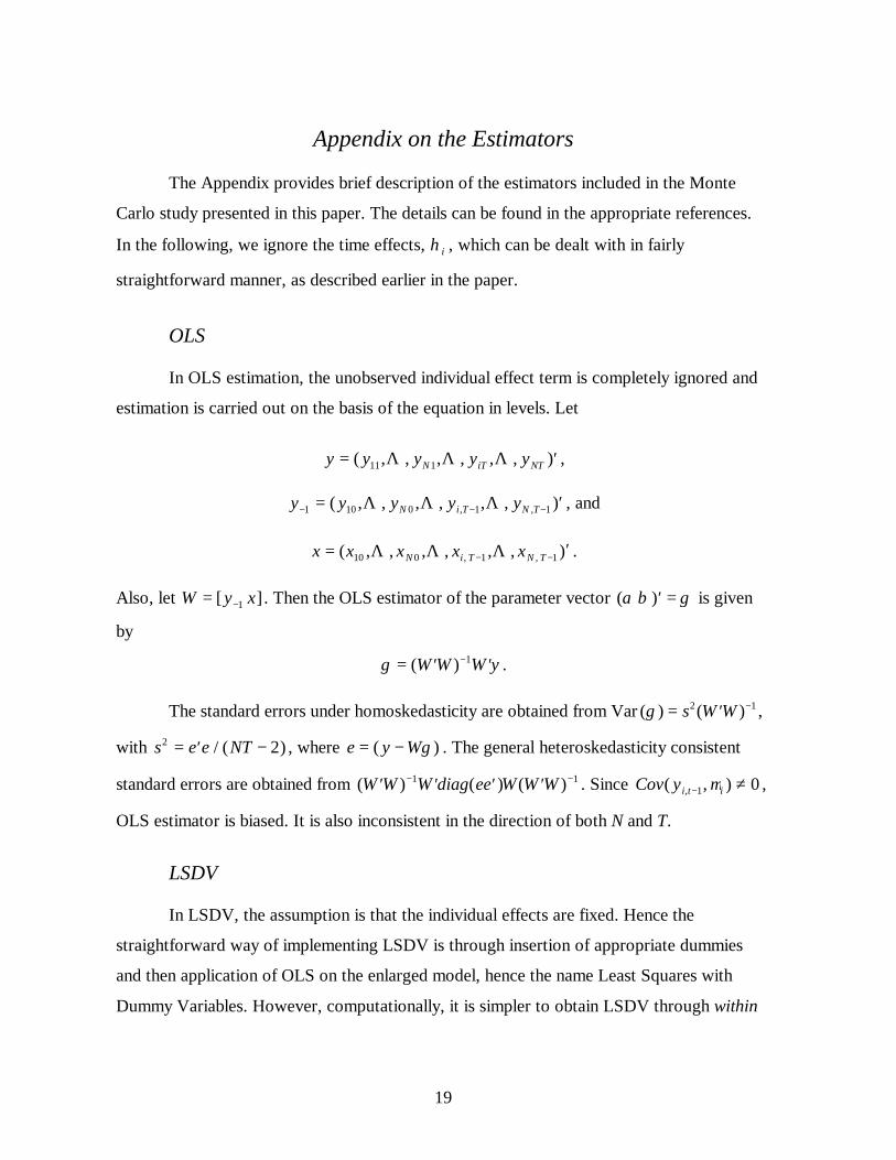
Appendix on the Estimators

The Appendix provides brief description of the estimators included in the Monte

Carlo study presented in this paper. The details can be found in the appropriate references.

In the following, we ignore the time effects, iη , which can be dealt with in fairly

straightforward manner, as described earlier in the paper.

OLS

In OLS estimation, the unobserved individual effect term is completely ignored and

estimation is carried out on the basis of the equation in levels. Let

y y y y yN iT NT= ′( , , , , , , )11 1Λ Λ Λ ,

y y y y yN i T N T− − −= ′1 10 0 1 1( , , , , , , ), ,Λ Λ Λ , and

),,,,,,( 1,1,010 ′= −− TNTiN xxxxx ΛΛΛ .

Also, let W y x= −[ ]1 . Then the OLS estimator of the parameter vector ( )α β γ′= is given

by

∃ ( )γ= ′ ′−W W W y1 .

The standard errors under homoskedasticity are obtained from Var ( ∃) ( )γ = ′ −s W W2 1 ,

with s e e NT2 2= ′ −/ ( ) , where e y W= −( ∃)γ . The general heteroskedasticity consistent

standard errors are obtained from ( ) ( ) ( )′ ′ ′ ′− −W W W diag ee W W W1 1 . Since Cov y i t i( , ), − ≠1 0µ ,

OLS estimator is biased. It is also inconsistent in the direction of both N and T.

LSDV

In LSDV, the assumption is that the individual effects are fixed. Hence the

straightforward way of implementing LSDV is through insertion of appropriate dummies

and then application of OLS on the enlarged model, hence the name Least Squares with

Dummy Variables. However, computationally, it is simpler to obtain LSDV through within

20

estimation. Averaging equation (1) over time and subtracting it from the original equation

yields

)()()( 1,1,1, iititiitiiit vvxxyyyy −+−+−=− −−− βα ,

where ∑∑∑∑=

−

=−

−

=−−

=====

T

titi

T

ttii

T

ttii

T

titi v

Tvx

Txy

Tyy

Ty

1

1

01,

1

01,1,

1

1and,

1,

1,

1. LSDV

estimation of the original model is equivalent to OLS estimation of the above equation.

Denote )(~and),(~),(~1,1,1,1,1, ititiititiiitit xxxyyyyyy −=−=−= −−−−− . Also, denote

~ (~ , , ~ , , ~ , , ~ )y y y y yN T NT= ′11 1 1Λ Λ Λ ,

~ (~ , , ~ , , ~ , , ~ ), ,y y y y yN T N T− − −= ′1 10 0 1 1 1Λ Λ Λ , and

)~,,~,,~,,~(~1,1,1010 ′= −− TNTN xxxxx ΛΛΛ .

Now, if ~ [~ ~]W y x= − 1 , then the LSDV estimator is given by

∃ ( ~ ~) ~γ= ′ ′−W W W y1 .

Clearly, Cov y y v vi t i it i[( ), ( )], ,− −− −1 1 is not equal to zero. This makes LSDV estimator

biased. It is also inconsistent in the direction of N. However, Amemiya (1967) shows that

LSDV for this model is consistent as ∞→T , and, if the errors are normally distributed,

LSDV is asymptotically equivalent to MLE. The standard errors of the LSDV estimates

under the assumption of homoskedasticity are obtained from Var s W W( ∃) ~ ( ~ ~)γ = ′ −2 1 , with

~ ~ ~ / ( )s e e NT N2 2= ′ − − , where ~ (~ ~ ∃)e y W= − γ .

Anderson and Hsiao Instrumental Variable (IV) Estimators

The two IV estimators proposed by Anderson and Hsiao (1981, 1982) both start by

differencing equation (1) to eliminate the individual effect term iµ . This yields

)()()( 1,2,1,2,1,1, −−−−−− −+−+−=− tiittititititiit vvxxyyyy βα

21

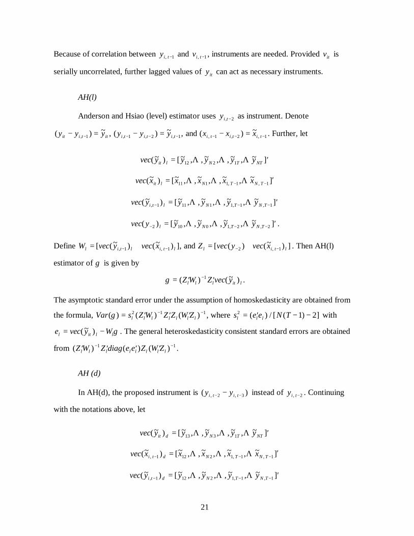
Because of correlation between 1, −tiy and 1, −tiv , instruments are needed. Provided itv is

serially uncorrelated, further lagged values of ity can act as necessary instruments.

AH(l)

Anderson and Hsiao (level) estimator uses yi t, − 2 as instrument. Denote

1,2,1,1,2,1,1,~)(and,~)(,~)( −−−−−−− =−=−=− titititititiittiit xxxyyyyyy . Further, let

vec y y y y yit l N T NT(~ ) [~ , , ~ , , ~ , ~ ]= ′12 2 1Λ Λ Λ

]~,~,,~,,~[)~( 1,1,1111 ′= −− TNTNlit xxxxxvec ΛΛΛ

vec y y y y yi t l N T N T(~ ) [~ , , ~ , , ~ , ~ ], , ,− − −= ′1 11 1 1 1 1Λ Λ Λ

vec y y y y yl N T N T( ) [~ , , ~ , , ~ , ~ ], ,− − −= ′2 10 0 1 2 2Λ Λ Λ .

Define ])~()([and],)~()~([ 1,21,1, ltilltiltil xvecyvecZxvecyvecW −−−− == . Then AH(l)

estimator of γ is given by

∃ ( ) (~ )γ= ′ ′−Z W Z vec yl l l it l1 .

The asymptotic standard error under the assumption of homoskedasticity are obtained from

the formula, Var s Z W Z Z W Zl l l l l l l( ∃) ( ) ( )γ = ′ ′ ′− −2 1 1 , where s e e N Tl l l2 1 2= ′ − −( ) / [ ( ) ] with

e vec y Wl it l l= −(~ ) ∃γ. The general heteroskedasticity consistent standard errors are obtained

from ( ) ( ) ( )′ ′ ′ ′− −Z W Z diag e e Z W Zl l l l l l l l1 1 .

AH (d)

In AH(d), the proposed instrument is )( 3,2, −− − titi yy instead of 2, −tiy . Continuing

with the notations above, let

vec y y y y yit d N T NT(~ ) [~ , , ~ , , ~ , ~ ]= ′13 3 1Λ Λ Λ

]~,~,,~,,~[)~( 1,1,12121, ′= −−− TNTNdti xxxxxvec ΛΛΛ

vec y y y y yi t d N T N T(~ ) [~ , , ~ , , ~ , ~ ], , ,− − −= ′1 12 2 1 1 1Λ Λ Λ

22

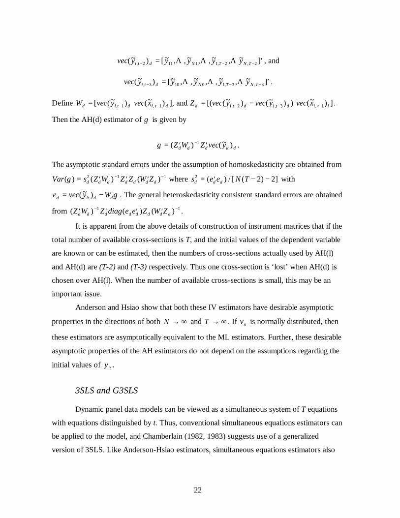
vec y y y y yi t d N T N T(~ ) [~ , , ~ , , ~ , ~ ], , ,− − −= ′2 11 1 1 2 2Λ Λ Λ , and

vec y y y y yi t d N T N T(~ ) [~ , , ~ , , ~ , ~ ], , ,− − −= ′3 10 0 1 3 3Λ Λ Λ .

Define ])~())~()~([(and],)~()~([ 1,3,2,1,1, ltidtidtiddtidtid xvecyvecyvecZxvecyvecW −−−−− −== .

Then the AH(d) estimator of γ is given by

∃ ( ) (~ )γ= ′ ′−Z W Z vec yd d d it d1 .

The asymptotic standard errors under the assumption of homoskedasticity are obtained from

Var s Z W Z Z W Zd d d d d d d( ∃) ( ) ( )γ = ′ ′ ′− −2 1 1 where s e e N Td d d2 2 2= ′ − −( ) / [ ( ) ] with

e vec y Wd it d d= −(~ ) ∃γ. The general heteroskedasticity consistent standard errors are obtained

from ( ) ( ) ( )′ ′ ′ ′− −Z W Z diag e e Z W Zd d d d d d d d1 1 .

It is apparent from the above details of construction of instrument matrices that if the

total number of available cross-sections is T, and the initial values of the dependent variable

are known or can be estimated, then the numbers of cross-sections actually used by AH(l)

and AH(d) are (T-2) and (T-3) respectively. Thus one cross-section is ‘lost’ when AH(d) is

chosen over AH(l). When the number of available cross-sections is small, this may be an

important issue.

Anderson and Hsiao show that both these IV estimators have desirable asymptotic

properties in the directions of both ∞→N and ∞→T . If itv is normally distributed, then

these estimators are asymptotically equivalent to the ML estimators. Further, these desirable

asymptotic properties of the AH estimators do not depend on the assumptions regarding the

initial values of ity .

3SLS and G3SLS

Dynamic panel data models can be viewed as a simultaneous system of T equations

with equations distinguished by t. Thus, conventional simultaneous equations estimators can

be applied to the model, and Chamberlain (1982, 1983) suggests use of a generalized

version of 3SLS. Like Anderson-Hsiao estimators, simultaneous equations estimators also

23

begin by first differencing the model to eliminate the individual effect term iµ . The system

therefore looks as follows.

)()()( 1,2,1,2,1,1, −−−−−− −+−+−=− TiiTTiTiTiTiTiiT vvxxyyyy βα Μ )()()( 12010112 iiiiiiii vvxxyyyy −+−+−=− βα

However, unlike AH and Arellano estimators, simultaneous equations estimators use only

itx ’s as instruments. If observations on 0iy ’s are not available, then the system may be

completed by adding a specification of 0iy in terms of itx ’s as follows.

iTiTii xxy υφφφ ++++= − 1,0100 Λ

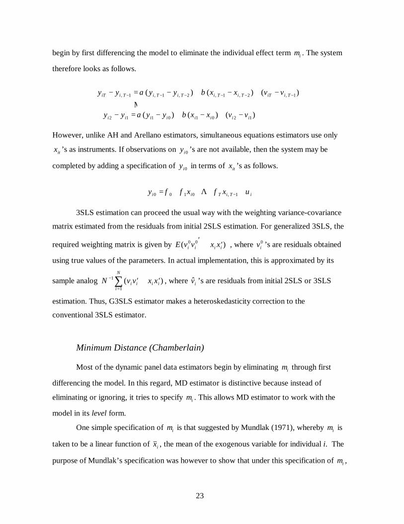
3SLS estimation can proceed the usual way with the weighting variance-covariance

matrix estimated from the residuals from initial 2SLS estimation. For generalized 3SLS, the

required weighting matrix is given by E v v x xi i i i( )0 0′⊗ ′ , where 0iv ’s are residuals obtained

using true values of the parameters. In actual implementation, this is approximated by its

sample analog N v v x xi i i ii

N−

=′⊗ ′∑1

1( ∃∃ ) , where iv ’s are residuals from initial 2SLS or 3SLS

estimation. Thus, G3SLS estimator makes a heteroskedasticity correction to the

conventional 3SLS estimator.

Minimum Distance (Chamberlain)

Most of the dynamic panel data estimators begin by eliminating iµ through first

differencing the model. In this regard, MD estimator is distinctive because instead of

eliminating or ignoring, it tries to specify iµ . This allows MD estimator to work with the

model in its level form.

One simple specification of iµ is that suggested by Mundlak (1971), whereby iµ is

taken to be a linear function of ix , the mean of the exogenous variable for individual i. The

purpose of Mundlak’s specification was however to show that under this specification of iµ ,

24

the GLS estimator under random effects assumption becomes equivalent to the LSDV

estimator under fixed effects assumption.

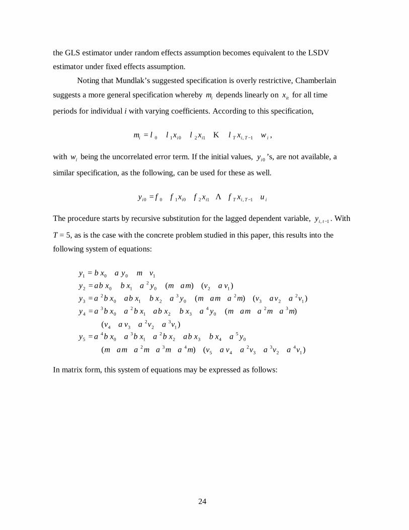
Noting that Mundlak’s suggested specification is overly restrictive, Chamberlain

suggests a more general specification whereby iµ depends linearly on itx for all time

periods for individual i with varying coefficients. According to this specification,

iTiTiii xxx ωλλλλµ +++++= − 1,12010 Κ ,

with iw being the uncorrelated error term. If the initial values, 0iy ’s, are not available, a

similar specification, as the following, can be used for these as well.

iTiTiii xxxy υφφφφ +++++= − 1,120100 Λ

The procedure starts by recursive substitution for the lagged dependent variable, 1, −tiy . With

T = 5, as is the case with the concrete problem studied in this paper, this results into the

following system of equations:

1001 vyxy +++= µαβ)()( 120

2102 vvyxxy ααµµαβαβ ++++++=

)()( 12

232

03

2102

3 vvvyxxxy ααµααµµαβαββα +++++++++=

)(

)(

13

22

34

320

4321

20

34

vvvv

yxxxxy

αααµαµααµµαβαββαβα

++++++++++++=

)()( 14

23

32

45432

05

4322

13

04

5

vvvvv

yxxxxxy

ααααµαµαµααµµαβαββαβαβα

+++++++++++++++=

In matrix form, this system of equations may be expressed as follows:

25

+

+++++++++

++

+

=

5

4

3

2

1

432

32

2

0

5

4

3

2

4

3

2

1

0

23

2

4

3

2

5

4

3

2

1

1

11

11

0000

000000

uuuuu

y

xxxxx

yyyyy

µ

ααααααααα

α

ααααα

βαββ

βααβ

βαβα

βαβα

βαββαβαβ

β

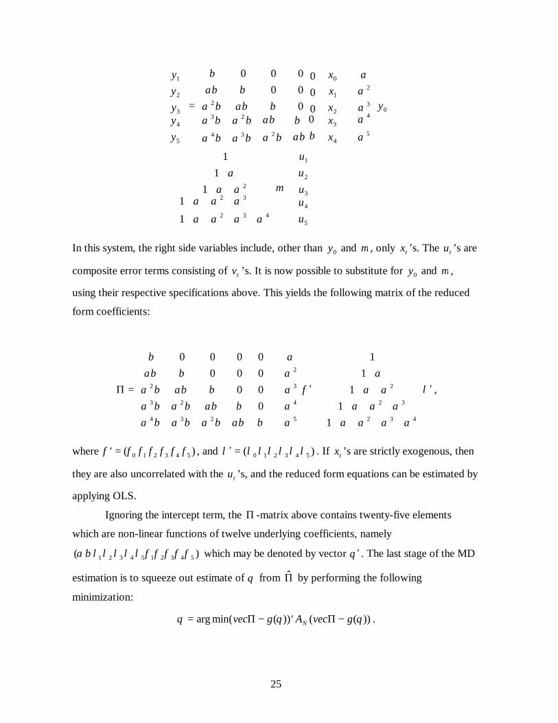
In this system, the right side variables include, other than 0y and µ , only tx ’s. The tu ’s are

composite error terms consisting of tv ’s. It is now possible to substitute for 0y and µ ,

using their respective specifications above. This yields the following matrix of the reduced

form coefficients:

λ

ααααααα

ααα

φ

ααααα

βαββαβαβαβαββαβα

βαββαβαβ

β

′

+++++++

+++

+′

+

=Π

432

32

2

5

4

3

2

234

23

2

11

11

1

0000000000

,

where ′=φ φ φφ φ φ φ( )0 1 2 3 4 5 , and )( 543210 λλλλλλλ =′ . If tx ’s are strictly exogenous, then

they are also uncorrelated with the tu ’s, and the reduced form equations can be estimated by

applying OLS.

Ignoring the intercept term, the Π -matrix above contains twenty-five elements

which are non-linear functions of twelve underlying coefficients, namely

)( 5432154321 φφφφφλλλλλβα which may be denoted by vector θ′. The last stage of the MD

estimation is to squeeze out estimate of θ from Π by performing the following

minimization:

∃ arg min( ∃ ( )) ( ∃ ( ))θ θ θ= − ′ −vec g A vec gNΠ Π .

26

Here )(θg is the vector-valued function mapping the elements of θ into )(Πvec .

Chamberlain shows that the optimal choice for the weighting matrix 1−NA is the inverse of

Ω Π Π Φ Φ= − − ′⊗ ′− −E y x y x x xi i i i x i i x[( )( ) ( ) ]0 0 1 1 ,

where 0Π is the matrix of true coefficients, and Φ x i iE x x= ′( ) . It may be noted that Ω is a

heteroskedasticity consistent weighting matrix. In actual implementation, it is replaced by its

consistent sample analog

∃ [( ∃ )( ∃ ) ( ) ]Ω Π Π= − − ′⊗ ′− − −∑N y x y x S x x Si ii

N

i i x i i x1 1 1 ,

where S x x Nx i ii

N

= ′=∑ /

1. Minimization can be conducted through an iterative routine. In the

current study, the modified Gauss-Newton algorithm was used for the purpose. Note that if

0iy ’s are known then the φ’s do not appear in the system, and the dimensions of the

estimation problem decreases.

AGMM1 and AGMM2

Extending Anderson-Hsiao’s idea, Arellano proposes using as instruments all further

lagged values of ity that qualify as instruments in view of serial uncorrelatedness of itv . The

number of instruments then differs depending on the time period for which the equation is

considered. Arellano uses the GMM framework to adopt a multi-equation approach and use

all the qualified instruments for each equation. The resulting block diagonal matrix of

instruments, iZ , can be seen as follows:

−

−−−

=

−−− 2,1,2,2

23

12

01

10

210

10

0

|

|00|00|00

00

0000000000

0000

00000000

TiTiTii

ii

ii

ii

ii

iii

ii

i

i

xxyy

xxxxxx

yy

yyyyy

y

ZΜΜ

ΛΟΜΛΛΛ

ΜΜΜΜΜΜΜΜ

27

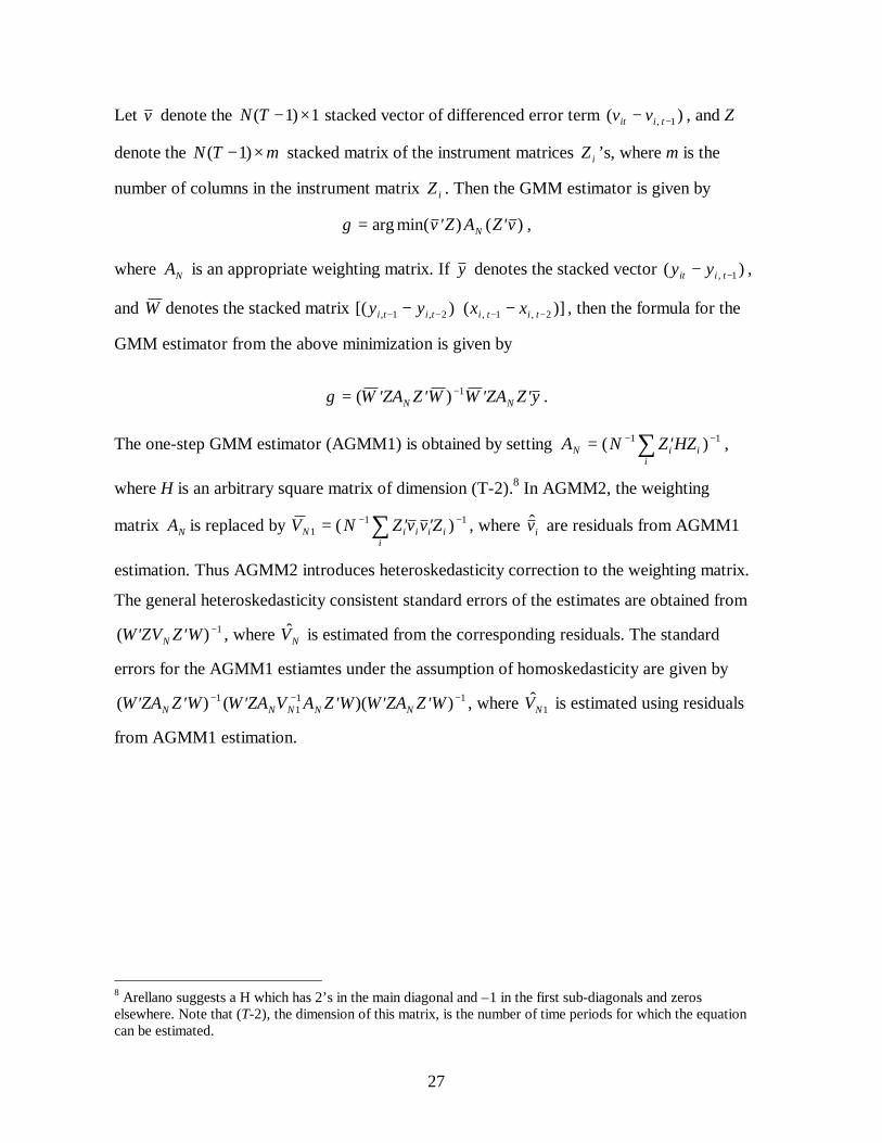
Let v denote the 1)1( ×−TN stacked vector of differenced error term )( 1, −− tiit vv , and Z

denote the mTN ×− )1( stacked matrix of the instrument matrices iZ ’s, where m is the

number of columns in the instrument matrix iZ . Then the GMM estimator is given by

∃ arg min( ) ( )γ= ′ ′v Z A Z vN ,

where NA is an appropriate weighting matrix. If y denotes the stacked vector )( 1, −− tiit yy ,

and W denotes the stacked matrix )]()[( 2,1,2,1, −−−− −− titititi xxyy , then the formula for the

GMM estimator from the above minimization is given by

∃ ( )γ= ′ ′ ′ ′−W ZA Z W W ZA Z yN N1 .

The one-step GMM estimator (AGMM1) is obtained by setting A N Z HZN i ii

= ′− −∑( )1 1 ,

where H is an arbitrary square matrix of dimension (T-2).8 In AGMM2, the weighting

matrix NA is replaced by ∃ ( ∃∃ )V N Z v v ZN ii

i i i11 1= ′ ′− −∑ , where iv are residuals from AGMM1

estimation. Thus AGMM2 introduces heteroskedasticity correction to the weighting matrix.

The general heteroskedasticity consistent standard errors of the estimates are obtained from

( ∃ )′ ′ −W ZV Z WN1 , where NV is estimated from the corresponding residuals. The standard

errors for the AGMM1 estiamtes under the assumption of homoskedasticity are given by

( ) ( ∃ )( )′ ′ ′ ′ ′ ′− − −W ZA Z W W ZA V A Z W W ZA Z WN N N N N1

11 1 , where 1NV is estimated using residuals

from AGMM1 estimation.

8 Arellano suggests a H which has 2’s in the main diagonal and –1 in the first sub-diagonals and zeroselsewhere. Note that (T-2), the dimension of this matrix, is the number of time periods for which the equationcan be estimated.

28

Appendix

Tables Showing Details of the Monte Carlo Distributions

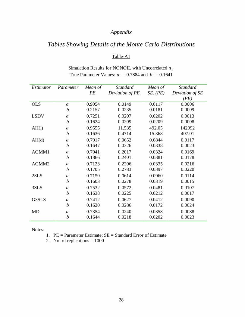
Table-A1

Simulation Results for NONOIL with Uncorrelated itνTrue Parameter Values: α = 0.7884 and β = 0.1641

Estimator Parameter Mean ofPE.

StandardDeviation of PE.

Mean ofSE. (PE)

StandardDeviation of SE

(PE)OLS α

β0.90540.2157

0.01490.0235

0.01170.0181

0.00060.0009

LSDV αβ

0.72510.1624

0.02070.0209

0.02020.0209

0.00130.0008

AH(l) αβ

0.95550.1636

11.5350.4714

492.0515.368

142092407.01

AH(d) αβ

0.79170.1647

0.06520.0326

0.08440.0338

0.01170.0023

AGMM1 αβ

0.70410.1866

0.20170.2401

0.03240.0381

0.01690.0178

AGMM2 αβ

0.71230.1705

0.22060.2783

0.03350.0397

0.02160.0220

2SLS αβ

0.71500.1603

0.06140.0278

0.09600.0319

0.01140.0015

3SLS αβ

0.75320.1638

0.05720.0225

0.04810.0212

0.01070.0017

G3SLS αβ

0.74120.1620

0.06270.0286

0.04120.0172

0.00900.0024

MD αβ

0.73540.1644

0.02400.0218

0.03580.0202

0.00880.0023

Notes:1. PE = Parameter Estimate; SE = Standard Error of Estimate2. No. of replications = 1000

29

Table-A2

Simulation Results for INTER with Uncorrelated itνTrue Parameter Values: α = 0.7925 and β = 0.1732



Mean ofSE. (PE)


(PE)OLS α

β0.91310.1936

0.01610.0253

0.01140.0184

0.00070.0019

LSDV αβ

0.72620.1741

0.02450.0215

0.02310.0215

0.00170.0009

AH(l) αβ

0.20010.1405

10.5760.4778

492.0410.086

7704.5167.80

AH(d) αβ

0.79420.1721

0.04280.0351

0.05840.0356

0.00600.0023

AGMM1 αβ

0.44060.1603

0.37410.2560

0.05680.0340

0.03410.0169

AGMM2 αβ

0.41790.1785

0.50810.3251

0.06500.0382

0.05810.0325

2SLS αβ

0.76800.1778

0.03240.0334

0.05250.0346

0.00420.0016

3SLS αβ

0.74640.1766

0.06060.0283

0.05320.0217

0.00980.0022

G3SLS αβ

0.72690.1766

0.06770.0307

0.04250.0165

0.00950.0030

MD αβ

0.73800.1749

0.02470.0217

0.03180.0189

0.00910.0027


30

Table-A3

Simulation Results for OECD with Uncorrelated itνTrue Parameter Values: α = 0.6294 and β = 0.0954



Mean ofSE. (PE)


(PE)OLS α

β0.76440.1908

0.03770.0587

0.02230.0350

0.00280.0045

LSDV αβ

0.61950.0940

0.01930.0382

0.01880.0389

0.00220.0030

AH(l) αβ

0.62810.0927

0.03300.0573

0.05670.0581

0.00930.0052

AH(d) αβ

0.63290.0938

0.04560.0619

0.06730.0648

0.01060.0069

AGMM1 αβ

0.56590.0884

0.14050.2322

0.03580.0455

0.02160.0280

AGMM2 αβ

0.57550.0789

0.19980.2922

0.03990.0510

0.02820.0394

2SLS αβ

0.51100.0946

0.09660.0556

0.20890.1104

0.04960.0094

3SLS αβ

0.54920.0905

0.16010.0639

0.07310.0432

0.03430.0077

G3SLS αβ

0.50440.0818

0.22540.1131

0.02760.0153

0.01790.0071

MD αβ

0.62140.0948

0.01720.0384

0.01140.0184

0.01670.0134


31

Table-A4

Simulation Results for NONOIL with MA(1) itνTrue Parameter Values: α = 0.7884 and β = 0.1641



Mean ofSE. (PE)


(PE)OLS α

β0.90380.2167

0.01560.0239

0.01200.0186

0.00060.0009

LSDV αβ

0.72410.1630

0.02410.0251

0.02150.0224

0.00130.0009

AH(l) αβ

0.27830.0918

5.16620.3746

41.2472.3581

184.5514.054

AH(d) αβ

0.67430.1605

0.06360.0328

0.07760.0322

0.00930.0017

AGMM1 αβ

0.70680.1878

0.20110.2481

0.03100.0389

0.01370.0209

AGMM2 αβ

0.70850.1727

0.21640.2783

0.03170.0404

0.01440.0279

2SLS αβ

0.71500.1597

0.06630.0299

0.09900.0329

0.01250.0015

3SLS αβ

0.76210.1638

0.05620.0249

0.05430.0238

0.01030.0018

G3SLS αβ

0.74560.1601

0.06840.0264

0.04610.0189

0.00910.0023

MD αβ

0.73410.1630

0.02800.0253

0.04150.0225

0.00980.0026

Notes:1. 1.PE = Parameter Estimate; SE = Standard Error of Estimate2. No. of replications = 1000

32

Table-A5

Simulation Results for INTER with MA(1) itνTrue Parameter Values: α = 0.7925 and β = 0.1732



Mean ofSE. (PE)


(PE)OLS α

β0.91290.1935

0.01610.0253

0.01140.0184

0.00070.0019

LSDV αβ

0.71920.1756

0.02450.0215

0.02310.0215

0.00170.0009

AH(l) αβ

0.97030.1717

1.86580.0945

8.76330.4108

24.0201.1130

AH(d) αβ

0.71690.1713

0.08050.0367

0.09810.0360

0.01520.0023

AGMM1 αβ

0.39990.2015

0.39680.2649

0.06350.0417

0.04040.0255

AGMM2 αβ

0.40000.2114

0.54660.3534

0.07340.0479

0.06720.0426

2SLS αβ

0.76790.1767

0.03570.0358

0.05510.0363

0.00450.0018

3SLS αβ

0.72950.1771

0.06170.0268

0.06060.0245

0.01250.0022

G3SLS αβ

0.71280.1770

0.07500.0318

0.04960.0185

0.01200.0028

MD αβ

0.72960.1740

0.02830.0262

0.03790.0215

0.01120.0030


33

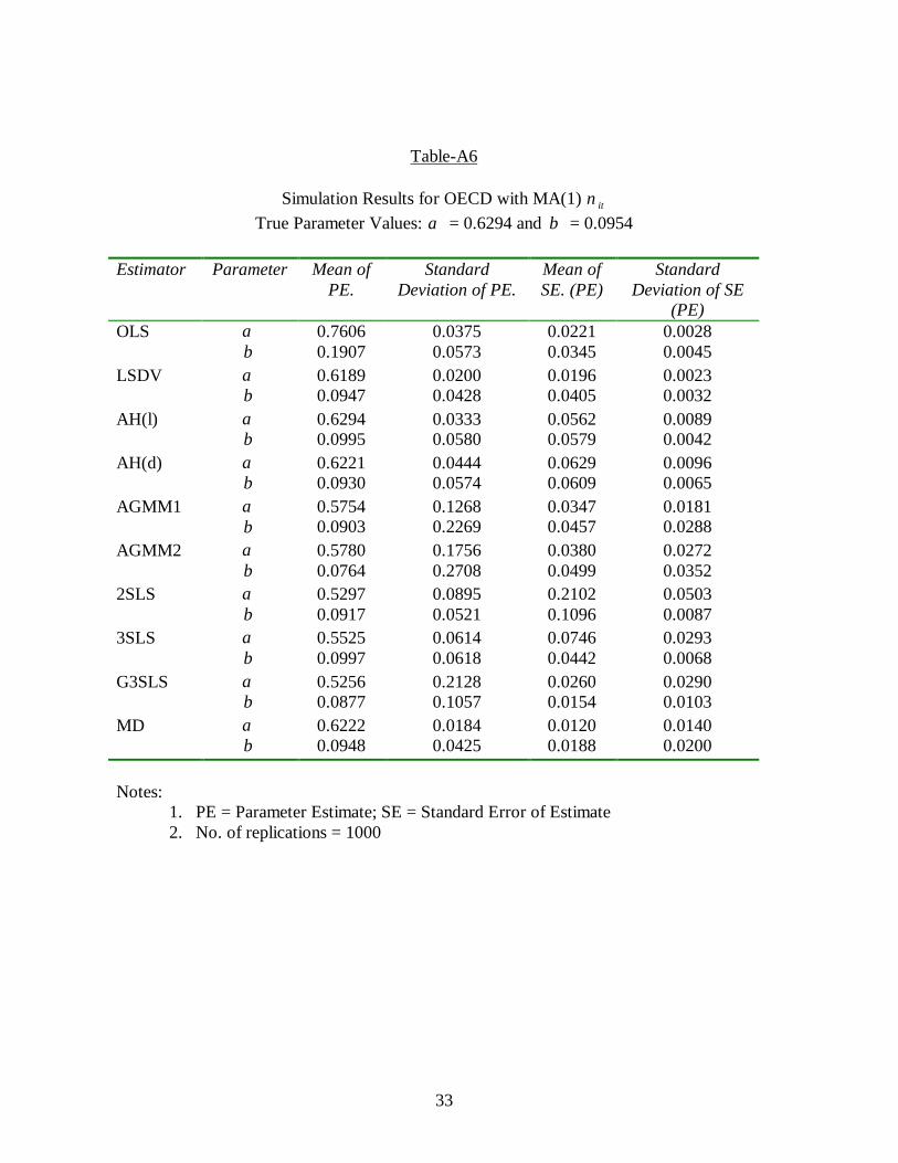
Table-A6

Simulation Results for OECD with MA(1) itνTrue Parameter Values: α = 0.6294 and β = 0.0954



Mean ofSE. (PE)


(PE)OLS α

β0.76060.1907

0.03750.0573

0.02210.0345

0.00280.0045

LSDV αβ

0.61890.0947

0.02000.0428

0.01960.0405

0.00230.0032

AH(l) αβ

0.62940.0995

0.03330.0580

0.05620.0579

0.00890.0042

AH(d) αβ

0.62210.0930

0.04440.0574

0.06290.0609

0.00960.0065

AGMM1 αβ

0.57540.0903

0.12680.2269

0.03470.0457

0.01810.0288

AGMM2 αβ

0.57800.0764

0.17560.2708

0.03800.0499

0.02720.0352

2SLS αβ

0.52970.0917

0.08950.0521

0.21020.1096

0.05030.0087

3SLS αβ

0.55250.0997

0.06140.0618

0.07460.0442

0.02930.0068

G3SLS αβ

0.52560.0877

0.21280.1057

0.02600.0154

0.02900.0103

MD αβ

0.62220.0948

0.01840.0425

0.01200.0188

0.01400.0200


34

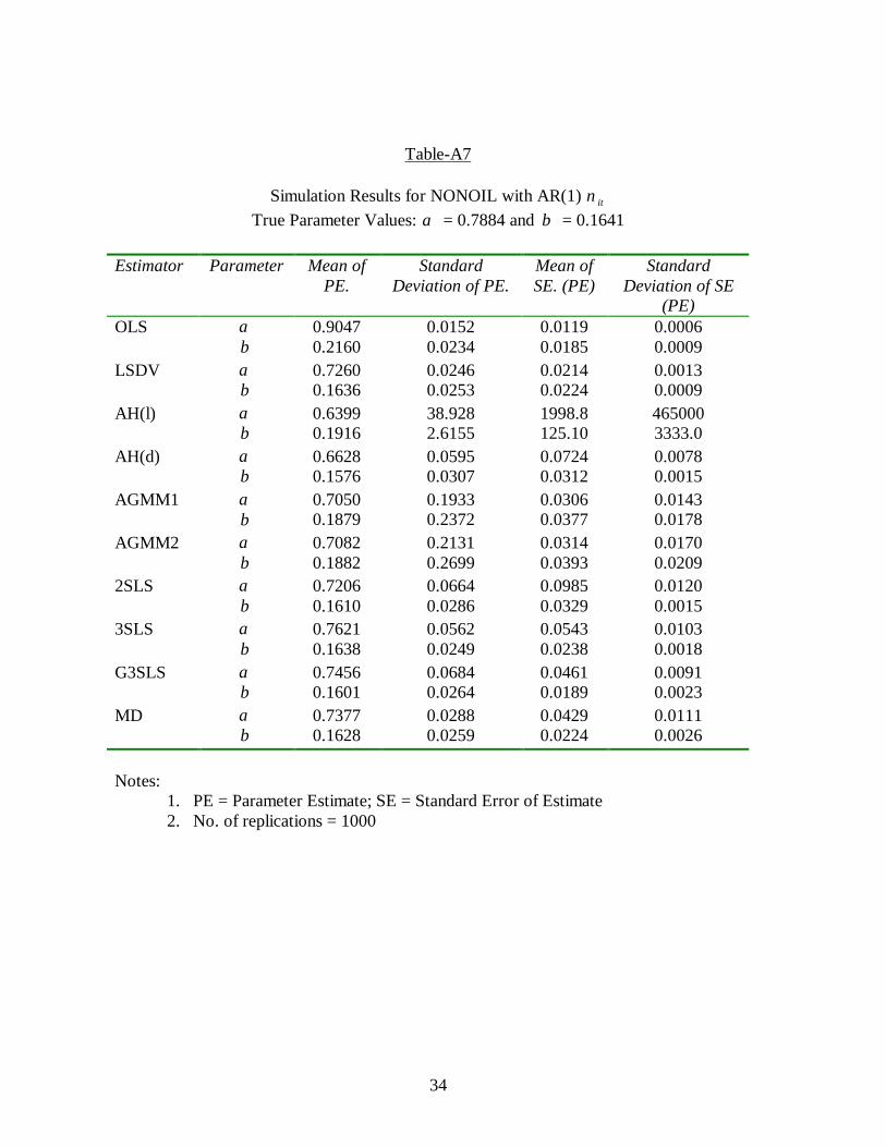
Table-A7

Simulation Results for NONOIL with AR(1) itνTrue Parameter Values: α = 0.7884 and β = 0.1641



Mean ofSE. (PE)


(PE)OLS α

β0.90470.2160

0.01520.0234

0.01190.0185

0.00060.0009

LSDV αβ

0.72600.1636

0.02460.0253

0.02140.0224

0.00130.0009

AH(l) αβ

0.63990.1916

38.9282.6155

1998.8125.10

4650003333.0

AH(d) αβ

0.66280.1576

0.05950.0307

0.07240.0312

0.00780.0015

AGMM1 αβ

0.70500.1879

0.19330.2372

0.03060.0377

0.01430.0178

AGMM2 αβ

0.70820.1882

0.21310.2699

0.03140.0393

0.01700.0209

2SLS αβ

0.72060.1610

0.06640.0286

0.09850.0329

0.01200.0015

3SLS αβ

0.76210.1638

0.05620.0249

0.05430.0238

0.01030.0018

G3SLS αβ

0.74560.1601

0.06840.0264

0.04610.0189

0.00910.0023

MD αβ

0.73770.1628

0.02880.0259

0.04290.0224

0.01110.0026


35

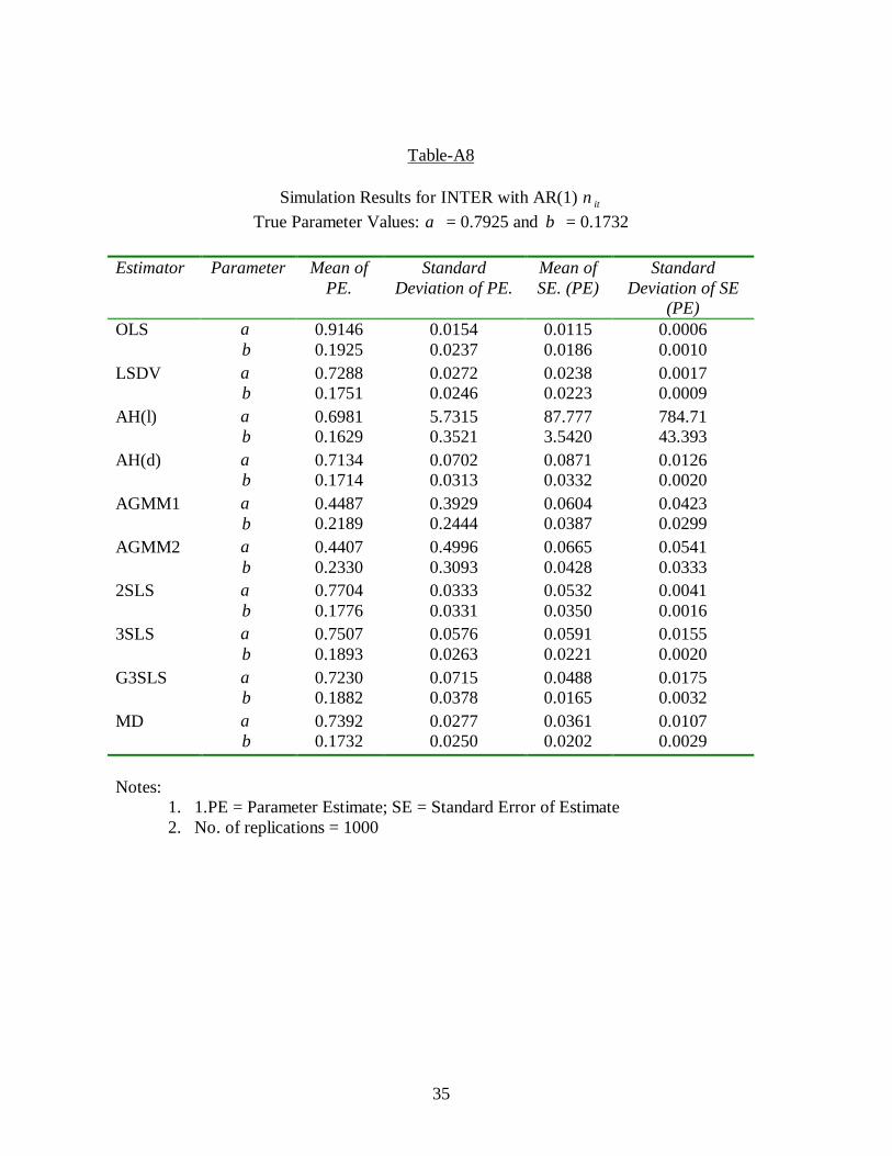
Table-A8

Simulation Results for INTER with AR(1) itνTrue Parameter Values: α = 0.7925 and β = 0.1732



Mean ofSE. (PE)


(PE)OLS α

β0.91460.1925

0.01540.0237

0.01150.0186

0.00060.0010

LSDV αβ

0.72880.1751

0.02720.0246

0.02380.0223

0.00170.0009

AH(l) αβ

0.69810.1629

5.73150.3521

87.7773.5420

784.7143.393

AH(d) αβ

0.71340.1714

0.07020.0313

0.08710.0332

0.01260.0020

AGMM1 αβ

0.44870.2189

0.39290.2444

0.06040.0387

0.04230.0299

AGMM2 αβ

0.44070.2330

0.49960.3093

0.06650.0428

0.05410.0333

2SLS αβ

0.77040.1776

0.03330.0331

0.05320.0350

0.00410.0016

3SLS αβ

0.75070.1893

0.05760.0263

0.05910.0221

0.01550.0020

G3SLS αβ

0.72300.1882

0.07150.0378

0.04880.0165

0.01750.0032

MD αβ

0.73920.1732

0.02770.0250

0.03610.0202

0.01070.0029

Notes:1. 1.PE = Parameter Estimate; SE = Standard Error of Estimate2. No. of replications = 1000

36

Table-A9

Simulation Results for OECD with AR(1) itνTrue Parameter Values: α = 0.6294 and β = 0.0954



Mean ofSE. (PE)


(PE)OLS α

β0.76290.1913

0.03780.0553

0.02210.0346

0.00280.0044

LSDV αβ

0.62080.0934

0.02080.0417

0.01920.0400

0.00220.0032

AH(l) αβ

0.63190.0965

0.03370.0586

0.05550.0571

0.00870.0049

AH(d) αβ

0.61920.0950

0.04590.0593

0.06490.0630

0.00950.0061

AGMM1 αβ

0.57700.0929

0.13990.2161

0.03500.0453

0.02000.0288

AGMM2 αβ

0.57620.0968

0.18770.2710

0.03780.0495

0.02510.0384

2SLS αβ

0.52150.0917

0.09640.0551

0.21360.1105

0.05250.0090

3SLS αβ

0.55290.0869

0.12750.0782

0.07780.0446

0.03370.0061

G3SLS αβ

0.54490.0973

0.16430.1427

0.02740.0165

0.01570.0079

MD αβ

0.62190.0966

0.01850.0435

0.01200.0191

0.02380.0161


37

References

Amemiya, T. (1967), “A Note on the Estimation of Balestra-Nerlove Models,” Technical

Report No. 4, Institute of Mathematical Studies in Social Sciences, Stanford

University.

Amemiya, T. (1971), “Estimation of the Variance in a Variance-Component Model,”

International Economic Review, 12:1-13.

Anderson, T. W. and C. Hsiao (1981), “Estimation of Dynamic Models with Error

Components,” Journal of American Statistical Association, 76:598-606.

Anderson, T. W. and C. Hsiao (1982), “Formulation and Estimation of Dynamic Models

Using Panel Data,” Journal of Econometrics, 18:47-82.

Arellano, M. (1989a), “On the Efficient Estimation of Simultaneous Equations with

Covariance Restrictions,” Journal of Econometrics, 42:247-265.

Arellano, M. (1989b), “An Efficient GLS Estimation of Triangular Models with

Covariance Restrictions,” Journal of Econometrics, 42:267-273.

Arellano, M. and S. Bond (1991), “Some Tests of Specification for Panel Data: Monte

Carlo Evidence and an Application to Employment Equations,” The Review of

Economic Studies, 58:277-297.

Balestra, P. and M. Nerlove (1966), “Pooling Cross-section and Time Series Data in the

Estimation of a Dynamic Model: The Demand of Natural Gas,” Econometrica,

34:585-612.

Bhargava, A. and J. D. Sargan (1983), “Estimating Dynamic Random Effects Models

from Panel Data Covering Short Time Periods,” Econometrica, 51:1635-1659.

38

Chamberlain, G. (1982), “Multivariate Regression Models for Panel Data,” Journal of

Econometrics, 18:5-46.

Chamberlain, G. (1983), “Panel Data,” in Z. Griliches and M. Intrilligator (editors),

Handbook of Econometrics, Vol. II., 1247-1318.

Mankiw, N. G., D. Romer, and D. Weil (1992), “A Contribution to the Empirics of

Growth,” Quarterly Journal of Economics, CVII: 407-437.

Nerlove, M. (1967), “Experimental Evidence on the Estimation of Dynamic Economic

Relations from a Time Series of Cross-sections, Economic Studies Quarterly,

18:42-74.

Nerlove, M. (1971), “Further Evidence on the Estimation of Dynamic Economic

Relations from a Time Series of Cross-sections,” Econometrica, 39:383-396.

Nickel, S. (1979), “Biases in Dynamic Models with Fixed Effects,” Econometrica,

49:1399-1416.

Sevestre, P. and Trognon, A. (1982), “A Note on Autoregressive Error Components

Models,” 8209, Ecole Nationale de la Statistique et de l’Administration

Economique et Unite de Recherche.

Summers, R. and A. Heston (1988), “A New Set of International Comparisons of Real

Product and Price Levels Estimates for 130 Countries, 1950-85,” Review of

Income and Wealth, XXXIV: 1-26.

Summers, R. and A. Heston (1991), “The Penn World Table (Mark 5): An Expanded Set

of International Comparisons, 1950-1988,” Quarterly Journal of Economics,

106: 327-368.

39

Abstract

This paper investigates the small sample properties of dynamic panel data estimators

as applied for estimation of growth convergence equation using Summers-Heston data set.

The Monte Carlo results show that estimates from different estimators do vary. Second,

those dynamic panel estimators which do not use further lagged dependent variable as

instruments perform better than the ones which do. These results together suggest that

investigators using panel estimators should try to check into the possible small sample bias

of their results. (JEL classification: C3, O4)

small sample performance of dynamic panel data estimators...

Documents